The Limited Macroeconomic Effects ofUnemployment Benefit Extensions∗

Gabriel Chodorow-ReichHarvard University and NBER

John CoglianeseHarvard University

Loukas KarabarbounisUniversity of Minnesota, FRB Minneapolis, and NBER

March 2018

Abstract

By how much does an extension of unemployment benefits affect macroeconomic

outcomes such as unemployment? Answering this question is challenging because U.S.

law extends benefits for states experiencing high unemployment. We use data revisions

to decompose the variation in the duration of benefits into the part coming from

actual differences in economic conditions and the part coming from measurement error

in the real-time data used to determine benefit extensions. Using only the variation

coming from measurement error, we find that benefit extensions have a limited influence

on state-level macroeconomic outcomes. We apply our estimates to the increase in

the duration of benefits during the Great Recession and find that they increased the

unemployment rate by at most 0.3 percentage point.

JEL-Codes: E24, E62, J64, J65.

Keywords: Unemployment Insurance, Measurement Error, Unemployment.

∗We are grateful to Robert Barro, Larry Katz, Andi Mueller, Emi Nakamura, five anonymous referees, and

participants in seminars and conferences for helpful comments. We thank Claudia Macaluso and Johnny Tang for

excellent research assistance, Thomas Stengle of the Department of Labor for help in understanding the unemploy-

ment insurance laws, and Bradley Jensen of the Bureau of Labor Statistics for help in understanding the process

for constructing state unemployment rates. Karabarbounis thanks the Alfred P. Sloan Foundation for generous

financial support. The views expressed herein are those of the authors and not necessarily those of the Federal

Reserve Bank of Minneapolis or the Federal Reserve System.

1 Introduction

Responding to the increase in unemployment during the Great Recession, the potential duration

of unemployment insurance (UI) benefits in the United States increased from 26 weeks to up

to 99 weeks. Recent studies have found mixed effects of these benefit extensions on individual

outcomes (Rothstein, 2011; Farber and Valletta, 2015; Johnston and Mas, Forthcoming). The

effect on macroeconomic outcomes has been even more controversial. According to one view,

by making unemployment relatively more attractive to the jobless, the extension of benefits

contributed substantially to the slow recovery of the labor market (Barro, 2010; Hagedorn,

Karahan, Manovskii, and Mitman, 2015). Others have emphasized the potential stimulus effects

of increasing transfers to unemployed individuals (Summers, 2010; Congressional Budget Office,

2012). Distinguishing between these possibilities has important implications for the design of

UI policy and for economists’ understanding of labor markets.

Quantifying the effects of UI benefit extensions on macroeconomic outcomes is challenging.

Federal law links actual benefit extensions in a state directly to state-level macroeconomic con-

ditions. This policy rule mechanically generates a positive correlation between unemployment

and benefit extensions, complicating the identification of any direct effect that benefit extensions

may have on macroeconomic outcomes.

To shed light on this policy debate, we propose a novel empirical design that exploits state

variation in benefit extensions caused by measurement error. Our results are inconsistent with

large effects of benefit extensions on state-level macroeconomic aggregates including unemploy-

ment, employment, vacancies, and worker earnings. Instead, we find that the extension of

benefits has only a limited influence on macroeconomic outcomes.

Our empirical approach starts from the observation that, at the state level, the duration of

UI benefits depends on the unemployment rate as estimated in real time. However, real-time

data provide a noisy signal of the true economic fundamentals. It follows that two states differ

in the duration of their UI benefits either because of differences in fundamentals or because

of measurement error. We use subsequent revisions of the unemployment rate to separate the

1

Table 1: April 2013 Example

Louisiana Wisconsin

Real-Time Data Unemployment Rate (Moving Average) 5.9% 6.9%

Duration of Benefit Extensions 14 Weeks 28 Weeks

Revised Data Unemployment Rate (Moving Average) 6.9% 6.9%

Duration of Benefit Extensions 28 Weeks 28 Weeks

UI Error -14 Weeks 0 Weeks

fundamentals from the measurement error. We then use the measurement error component of

UI benefit extensions to identify the effects of benefit extensions on state-level macroeconomic

aggregates. Effectively, our strategy exploits the randomness in the duration of benefits with

respect to economic fundamentals caused by measurement error in the fundamentals.

Table 1 uses the example of Louisiana and Wisconsin in April 2013 to illustrate our approach.

Under the 2008 emergency compensation program, the duration of benefits in a state increased

by 14 additional weeks if a moving average of the state’s unemployment rate exceeded 6 percent.

The unemployment rate measured in real time in Louisiana was 5.9 percent while that in

Wisconsin was 6.9 percent, resulting in an additional 14 weeks of potential benefits in Wisconsin

relative to Louisiana. However, data revised as of 2015 show that both states actually had the

same unemployment rate of 6.9 percent. According to the revised data, both states should have

qualified for the additional 14 weeks. We refer to the 14 weeks that Louisiana did not receive

as a “UI error.” This error reflects mismeasurement of the economic fundamentals rather

than differences in fundamentals between the two states and, therefore, provides variation to

identify the effects of UI benefit extensions on state aggregates. The actual unemployment

rate (from the revised data as of 2015) evolved very similarly following the UI error, declining

2

by roughly 0.2 percentage point between April and June 2013 in both states. Our empirical

exercise amounts to asking whether this apparent limited influence of extending benefits on

unemployment generalizes to a larger sample.

We begin our analysis by discussing relevant institutional details of the UI system, the

measurement of real-time and revised state unemployment rates, and the UI errors that arise

because of differences between real-time and revised data. The Bureau of Labor Statistics

(BLS) constructs state unemployment rates by combining a number of state-level data sources

using a state space model. Revisions to state unemployment rates occur due to revisions to

the input data, the use of the full time series of available data in the state space estimation

at the time of the revision, and the introduction of technical improvements in the statistical

model itself. Of these, the technical improvements account for the largest share of the variation

in the measurement error in the unemployment rate. The unemployment rate measurement

error gives rise to more than 600 state-month cases between 1996 and 2015 in which, as in the

example of Louisiana and Wisconsin in April 2013, the duration of benefits using the revised

data differs from the actual duration of benefits. Almost all of these UI errors occur during

the Great Recession. This concentration reflects both the additional tiers of benefits duration

created by the 2008 emergency compensation program and the fact that most states experienced

unemployment rates high enough for measurement errors to affect their eligibility for extended

benefits. Once a UI error occurs, it takes on average nearly 4 months to revert to zero.

We estimate impulse responses of state-level labor market variables to an unexpected inno-

vation in the UI error. Our identifying assumptions are that innovations in the UI error occur

randomly with respect to the true economic fundamentals and that the revised unemployment

rate measures the true economic fundamentals in the state. Our main result is that innovations

in the UI error have negligible effects on state-level unemployment, employment, vacancies, and

worker earnings. In the baseline specification, a one-month increase in the maximum potential

duration of benefits generates at most a 0.02 percentage point increase in the state unemploy-

ment rate. Crucially, a positive UI error innovation raises the fraction of the unemployed who

3

receive UI benefits by a statistically significant and an economically reasonable magnitude, with

the additional recipients being in the tiers affected by the error. Therefore, our results do not

reflect a failure of UI errors to lead to a larger fraction of unemployed receiving benefits. They

simply reflect the small macroeconomic effects of an increase in UI eligibility and receipt.

These impulse responses answer the question of what would happen if a state increased

the duration of unemployment benefits around the neighborhood of a typical UI error, or by

about 3 months after a state has already extended benefits by nearly one year. To assess the

informativeness of these estimates for other types of policies, we examine the heterogeneity of

responses with respect to the initial level of benefit duration and the persistence of the UI error.

The responses of labor market variables such as unemployment and vacancies do not vary along

either dimension. Therefore, a linear extrapolation of our estimates provides a reasonable guide

to the macroeconomic effects of longer extensions. Taking the upper bound of our preferred

specification, we find that extending benefits from 26 to 99 weeks increases the unemployment

rate by at most 0.3 percentage point.

We show the robustness of our results to the inclusion of a number of controls into the

baseline specification and to alternative specifications. Most important, a concern with using

revisions in the unemployment rate to construct UI errors is that the incorporation of the full

time series of data in the revision process makes the unemployment rate revision in month t

partly dependent on realizations of variables after month t. To make sure this aspect of the

revision process does not affect our results, we add to our regression controls for linear and non-

linear functions of the unemployment rate measurement error. The responses of labor market

variables remain similar to our baseline estimates, reflecting the fact that this aspect of the

revision process contributes very little to the variation in the unemployment rate measurement

error. Further, we develop an alternative series of UI errors using sampling error in the Current

Population Survey (CPS). We infer the sampling error from the difference between a measure

of the population eligible for regular benefits in the CPS and administrative data on UI receipt.

Constructing UI errors based only on this more restrictive source of measurement error implies

4

that UI errors do not depend on realizations of variables in future dates. We continue to find a

limited effect of unemployment benefit extensions on labor market outcomes using this approach.

Finally, we derive a bound for the consistency of our estimator when the revised data still

contain measurement error. Intuitively, the bound depends on the measurement error in the

revised data relative to that in the real-time data. We show that the macroeconomic effects

of benefit extensions are small so long as the revised data measure true economic conditions

at least as well as the real-time data and provide empirical support for this condition from

horse-race regressions in which measures of consumer spending and survey attitudes and beliefs

load on the revised but not on the real-time unemployment rate.

In the last part of the paper we complement our empirical results by analyzing a DMP

model (Diamond, 1982; Mortensen and Pissarides, 1994) augmented with a UI policy. The model

provides an alternative approach to considering larger extensions in the duration of benefits and

allows anticipation effects by workers and firms to differ according to whether a benefit extension

is caused by a transitory UI error or by a persistent increase in unemployment that triggers the

extension. As well known in the literature, the effect of UI policy on macroeconomic outcomes

depends crucially on the level of the opportunity cost of employment. We show that with a low

level of the opportunity cost of employment, such as the one estimated in Chodorow-Reich and

Karabarbounis (2016), a one-month UI error innovation leads to a less than 0.02 percentage

point increase in the unemployment rate, a magnitude similar to our empirical estimates. To

mimic the U.S. experience in the aftermath of the Great Recession, we subject the model to a

sequence of large negative shocks that increase unemployment from below 6 percent to roughly

10 percent and increase the duration of benefits from 6 months to 20 months. Removing benefit

extensions leads to a decline in the unemployment rate by at most 0.3 percentage point in the

model. Thus, both a linear extrapolation of the empirical results and the model exercise suggest

a small response of unemployment to the extension of benefits around the Great Recession.

The economic literature on the effects of benefit extensions has followed two related lines of

inquiry. Motivated in part by a partial equilibrium optimal taxation result linking the optimal

5

provision of UI to individual search behavior (Baily, 1978; Chetty, 2006), a microeconomic

literature has studied how various aspects of UI policy affects individual labor supply (for a

survey see Krueger and Meyer, 2002). Studies which find a small effect of benefit extensions

following the Great Recession on individual job finding rates and unemployment duration include

Rothstein (2011) and Farber and Valletta (2015), while Johnston and Mas (Forthcoming) find

somewhat larger effects in a study of a single benefit cut in Missouri in 2011.1

The macroeconomic effects of UI benefits concern their effect on aggregate unemployment.2

Economic theory does not provide a one-to-one mapping between the magnitude of the microe-

conomic and macroeconomic effects. For example, in a standard DMP model with exogenous

job search effort and Nash bargaining, an increase in UI benefits raises workers’ outside options,

putting an upward pressure on wages and depressing firm vacancy creation. Exogenous search

effort implies a zero microeconomic effect, but the decline in total vacancies generates a rise in

total unemployment, i.e. a non-zero macroeconomic effect (Hagedorn, Karahan, Manovskii, and

Mitman, 2015). Alternatively, in models with job rationing, large microeconomic effects could

be consistent with small macroeconomic effects if the job finding rate of UI recipients falls but

that of non recipients rises (Levine, 1993; Landais, Michaillat, and Saez, 2015; Lalive, Landais,

and Zweimuller, 2015). Crepon, Duflo, Gurgand, Rathelot, and Zamora (2013) provide exper-

imental evidence that such displacement effects occur in the related setting of job placement

assistance programs.

A number of papers starting with Hagedorn, Karahan, Manovskii, and Mitman (2015,

HKMM) and Hagedorn, Manovskii, and Mitman (2015, HMM) use a county border discon-

tinuity design to estimate the macroeconomic effects of UI benefit extensions. Different from

our results, HKMM and HMM find a large positive effect of benefit extensions on unemployment.

1Schmieder, von Wachter, and Bender (2012) and Kroft and Notowidigdo (2015) show that the effect of UIbenefit extensions on unemployment duration becomes smaller during recessions.

2Our estimates of the macroeconomic effects are particularly informative for general equilibrium models withUI policy. See Hansen and Imrohoroglu (1992), Krusell, Mukoyama, and Sahin (2010), and Nakajima (2012) forearlier general equilibrium analyses of unemployment insurance policy. Landais, Michaillat, and Saez (2015) andKekre (2016) extend the Baily-Chetty partial equilibrium optimal UI formula to a general equilibrium setting andshow how it depends on the macroeconomic effects of benefit extensions.

6

However, the subsequent literature has challenged these findings. Hall (2013) first pointed out

problems that arise from the imputation of the unemployment rate at the county level and raised

conceptual questions about the identification strategy in HKMM. Amaral and Ice (2014) argue

the results in HKMM are sensitive to changes in the data sources and the specification, points

developed further in Boone, Dube, Goodman, and Kaplan (2016) and Dieterle, Bartalotti, and

Brummet (2016). Boone, Dube, Goodman, and Kaplan (2016) find near zero effects of UI exten-

sions on employment using a county border design and a more flexible empirical model. They

further show that using newer vintages of the unemployment data substantially reduces or elim-

inates the positive effect of benefit extensions on unemployment found in HKMM and HMM.3

Dieterle, Bartalotti, and Brummet (2016) point out that shocks triggering UI extensions in one

state may not affect neighboring countries similarly because population does not concentrate at

the border. They refine the border-county-pair strategy by controlling for polynomials in the

distance to the border and find a small response of unemployment to benefit extensions. Finally,

both Dieterle, Bartalotti, and Brummet (2016) and Marinescu (2017) cite job search spillovers

across counties to question the appropriateness of a border design to study UI extensions.

Other papers using cross-state variation find mixed macroeconomic effects. Johnston and

Mas (Forthcoming) use a sudden change in benefits in Missouri to estimate both the microeco-

nomic and macroeconomic effects. They estimate macroeconomic effects of similar magnitude

to the microeconomic effects, but their estimate of the macroeconomic effect depends on a

difference-in-difference research design with Missouri the only treated observation. Marinescu

(2017) uses data from a large job board and documents an insignificant effect of benefit dura-

tion on vacancies. Relative to this literature, ours is the first paper to use quasi-experimental

cross-state variation to estimate the macroeconomic effect of UI extensions on unemployment.

3For example, Boone, Dube, Goodman, and Kaplan (2016) find that HMM’s estimated effect falls by three-quarters and becomes statistically indistinguishable from zero using the newer data. They also forcefully questionthe assumptions underlying the quasi-forward differencing procedure used in HKMM. As they point out, if the trueeffect of UI extensions were to cause unemployment to slightly decrease, applying the quasi-differencing procedurewould nonetheless cause a researcher to conclude benefit extensions increase unemployment.

7

2 Unemployment Insurance in the United States

The maximum number of weeks of UI benefits available in the United States varies across states

and over time. Regular benefits in most states provide 26 weeks of compensation, with a range

between 13 and 30 weeks. The existence of regular UI benefits does not depend on economic

conditions in the state. Extended benefits (EB) and emergency compensation provide additional

weeks of benefits during periods of high unemployment in a state. The EB program has operated

since 1970 and is 50 percent federally funded except for the period 2009-2013 when it became

fully federally funded. Emergency compensation programs are authorized and financed on an

ad hoc basis by the federal government. In our sample (1996-2015), the Temporary Emergency

Unemployment Compensation (TEUC) program operated between March 2002 and December

2003 and the Emergency Unemployment Compensation (EUC) program operated between July

2008 and December 2013. We refer to the combination of EB and emergency compensation as

UI benefit extensions.

Whether a state qualifies for benefit extensions typically depends on the unemployment rate

exceeding some threshold. Two measures of unemployment arise in the laws governing these

extensions. The insured unemployment rate (IUR) is the ratio of recipients of regular benefits

to employees covered by the UI system. The total unemployment rate (TUR) is the ratio of

the total number of individuals satisfying the official definition of not working and on layoff

or actively searching for work to the total labor force. To avoid high frequency movements

in the available benefit extensions, both the IUR and the TUR enter as three-month moving

averages into the trigger formulas determining extensions. A trigger may also contain a lookback

provision which requires that the indicator exceed its value during the same set of months in

prior years. Appendix A.1 lists the full set of benefit extension programs, tiers, and triggers in

operation during our sample.

Not every unemployed individual qualifies for regular benefits, with eligibility determined

by reason for separation from previous employer, earnings over the previous year, and search

effort. An individual becomes eligible to receive benefits under EB or an emergency program

8

only after qualifying for and exhausting entitlement under regular benefits. Any individuals

who have exhausted eligibility under all previous tiers become immediately eligible to receive

benefits when their state triggers onto a new tier. Conversely, as soon as a state triggers off a

tier all individuals lose eligibility immediately regardless of whether they had begun to collect

benefits on that tier.

3 Empirical Design

We organize the discussion of our empirical methodology around a linear relationship between

a labor market variable ys,t+h observed in state s at date t + h, the maximum duration of

unemployment benefit receipt in the state at date t, which we denote as T ∗s,t, and all other

influences of the labor market variable es,t+h:

ys,t+h = β(h)T ∗s,t + es,t+h. (1)

Two main challenges arise in using equation (1) to estimate the causal effect β(h) of extending

benefits on state-level labor market outcomes. First, the extension of benefits depends on labor

market outcomes such as the state unemployment rate which induces a correlation between T ∗s,t

and es,t+h. In Section 3.1 we separate the benefit duration T ∗s,t into the part which depends

on true economic fundamentals in the state and the part which depends on measurement error

in the fundamentals and address this identification challenge by using only the latter part in

equation (1). Second, labor market variables such as the unemployment rate and vacancies

may depend not only on contemporaneous but also on past and future values of the duration of

benefit extensions. To the extent that the duration of benefits is autocorrelated over time, this

again induces a correlation between T ∗s,t and es,t+h. Section 3.2 explains how we address this

issue of serial correlation in the duration of benefits.

3.1 Endogeneity of Benefit Duration

The key idea underlying our approach is to use the variation in the duration of benefits caused

only by measurement error in state-level labor market outcomes. To implement this idea, we

9

decompose the benefit duration T ∗s,t into the part which depends on true economic fundamentals

in the state, Ts,t, and the part which depends on measurement error in the fundamentals, Ts,t.

Let fs,t(.) be the UI law which maps a history of unemployment rates in a state s into the

maximum duration of UI benefit extensions in the state. The time subscript t on the function

indicates that the mapping can change due to temporary legislation such as an emergency

compensation program. As described in Section 2, whether a state extends its duration of

benefits or not depends on the most recently reported or “real-time” estimate of the state-level

unemployment rate:

T ∗s,t = fs,t(u∗s,t−1

), (2)

where u∗s,t−1 denotes the real-time unemployment rate reported in month t for the latest available

month, t− 1.4

The reported unemployment rate in real time, u∗s,t, may deviate from the true unemployment

rate, us,t, because of measurement error, denoted by us,t = u∗s,t − us,t. Our empirical strategy

exploits variation in this measurement error to extract the component of benefit extensions which

is uncorrelated with state economic conditions. More formally, we first define a hypothetical

duration of benefit extensions, Ts,t, based on the true unemployment rate us,t and the same

function fs,t(.) that appears in equation (2):

Ts,t = fs,t (us,t−1) . (3)

We then define the UI error Ts,t from the relationship:

T ∗s,t = Ts,t + Ts,t. (4)

4For expositional reasons, we simplify a few details in writing monthly UI duration as a function of the previousmonth’s unemployment rate. The actual determination of UI benefit extensions eligibility occurs weekly and isbased on unemployment rate data available at the start of the week. The BLS typically releases the real-time statetotal unemployment rate data for month t − 1 around the 20th day of month t. Therefore, for the first weeks ofmonth t the most recent real-time unemployment rate which enters into the eligibility determination is for montht−2 while for the last weeks the most recent unemployment rate affecting eligibility is for month t−1. We aggregatein the text to a monthly frequency and capture the reporting lag for the real-time data by writing UI benefits inmonth t as a function of the unemployment rate in month t − 1. Next, as we discuss in Appendix A.1, benefitduration typically depends on a three month moving average of unemployment rates and may also depend on a“lookback” to the unemployment rate 12 and 24 months before, so that further lags of the unemployment rates alsoenter into the eligibility determination. Third, duration also depends on the insured unemployment rate, althoughthis trigger binds very rarely in our sample. While we appropriately take into account all of these details in ourimplementation, they do not affect the general econometric approach so we omit them in the main text for clarity.

10

Equation (4) shows that variation in the actual duration of benefit extensions T ∗s,t comes from

the component Ts,t which depends on the true economic fundamentals and from the component

Ts,t which reflects measurement error in the state unemployment rate. Our approach is to use

the part of the variation in T ∗s,t in regression (1) induced only from the UI error Ts,t to identify

the effects of benefit extensions on state-level outcomes. The remainder of this section discusses

how we construct the measurement error component Ts,t.

3.1.1 Measurement of State Unemployment Rates

A key step in our methodology is to use the revised unemployment rate to proxy for the true

unemployment rate us,t used in equation (3) to construct Ts,t.5 We now discuss the measurement

of the real-time and revised unemployment rates which underlie our construction of Ts,t. The

Local Area Unemployment Statistics (LAUS) program at the Bureau of Labor Statistics (BLS)

produces estimates of state-level unemployment rates. Unlike the national unemployment rate,

which derives directly from counts from the Current Population Survey (CPS) of households,

state unemployment rates incorporate auxiliary information to overcome the problem of small

sample sizes at the state level (roughly 1,000 labor force participants for the median state).

Better source data and improved statistical methodology imply substantial revisions in the

estimated unemployment rate over time.

Real-time unemployment rate u∗s,t. The real-time unemployment rate is calculated as the

ratio of real-time unemployment to real-time unemployment plus employment. The BLS uses a

state space filter to estimate separately real-time counts of unemployed and employed persons

(see Appendix A.2 for additional details). For unemployment the observed variables are the

CPS count of unemployed individuals in the state and the number of insured unemployed. For

employment the observed variables are the CPS count of employed individuals and the level of

5We later show that our main conclusions remain unchanged if the revised unemployment rate also containsmeasurement error and we provide additional results using an alternative proxy of the true unemployment rate.While the IUR also enters into the determination of T ∗s,t, the real-time IUR uses as inputs administrative data onUI payments and covered employment and contains minimal measurement error, with a standard deviation of thereal-time error in the IUR of 0.02 percentage point. Since revisions in the IUR do not meaningfully affect Ts,t wedo not discuss them further.

11

payroll employment in the state from the Current Employment Statistics (CES) program. From

2005 to 2014, the procedure also included a real-time benchmarking constraint that allocated

pro rata the residual between the sum of filter-based levels across states and the total at the

Census division or national level. Finally, in 2010 the BLS began applying a one-sided moving

average filter to the state space filtered and benchmarked data.

Revised unemployment rate us,t. The BLS publishes revisions of its estimates of the state

unemployment rates. Revisions occur for three reasons. First, the auxiliary data used in the

estimation – insured unemployment and payroll employment – are updated with comprehensive

administrative data not available in real time.6 Second, the BLS incorporates the entire time

series available at the time of the revision into its model, replacing the state space filter with

a state space smoother and the one-sided moving-average filter with a symmetric filter. Third,

the BLS periodically updates its estimation procedure to reflect methodological improvements.

Most recently, in 2015 the BLS replaced the external real-time benchmarking constraint with

a benchmarking constraint internal to the state space model, improved the treatment of state-

specific outliers in the CPS, and improved the seasonal adjustment procedure. Bureau of Labor

Statistics (2015) describes these changes as resulting in “more accurate and reliable estimates.”

We investigate the importance of different components of the revision process in Appendix A.2

by regressing the unemployment rate measurement error us,t on the components. We find that

the 2015 methodological update and the treatment of outliers account for the largest amount of

the variation in us,t. Importantly, the incorporation of the full time series at the time of revision

accounts for very little of the variation in us,t.

3.1.2 Implementation

To separate T ∗s,t into the component Ts,t based on the revised unemployment rate data and

the UI error Ts,t, we use the weekly trigger notices produced by the Department of Labor

6The revisions to the insured unemployment data reflect corrections of the administrative records, explainingwhy they are quite small. The annual revision of the CES state employment data replaces state-level real-timemonthly employment based on a survey of approximately 400,000 establishments with administrative data derivedfrom tax records covering a virtual universe of private sector employment.

12

Table 2: Accuracy of Our Algorithm for Calculating UI Benefit Extensions

TEUC02 EUC08 EB Total

2002-2003 2008-2013 1996-2007 2008-2015

Original Trigger NoticesSame as our algorithm 3982 14291 25541 19915 63729Different from our algorithm 18 9 9 35 71

Corrected Trigger NoticesSame as our algorithm 3999 14300 25548 19946 63793Different from our algorithm 1 0 2 4 7

Notes: The table reports the number of state-weeks where applying our algorithm to real-time unemployment ratedata gives the same UI benefit tier eligibility as the published DOL trigger notices. The top panel compares ouralgorithm to the raw trigger notices. In the bottom panel, we have corrected the information in the raw triggernotices when we find conflicting accounts in either contemporary media sources or in the text of state legislation.

(DOL). The DOL produces each week a trigger notice that contains for each state the most

recent available moving averages of IUR and TUR, the ratios of IUR and TUR relative to

previous years, and information on whether a state has any weeks of EB available and whether

it has adopted optional triggers for EB status. During periods with emergency compensation

programs, the DOL also produces separate trigger notices with the relevant input data and

status determination for the emergency programs. We scraped data for EB notices from 2003-

2015 and for the EUC 2008 programs from the DOL’s online repository. The TEUC notices

are not available online but were provided to us by the DOL. Finally, the DOL library in

Washington, D.C. contains print copies of trigger notices before 2003, which we scanned and

digitized.7 We augment these data with monthly real-time unemployment rates by digitizing

archived releases of the monthly state and local unemployment reports from the BLS.

We use the revised unemployment data as of 2015 as inputs into the trigger formulas de-

7The URL for the online data is http://www.oui.doleta.gov/unemploy/claims_arch.asp. The library couldnot locate notices for part of 1998. We also digitized notices for the EUC program in operation between 1991 and1994. However, we found only few non-zero UI errors. We, therefore, exclude this period from our analysis and startin 1996, which is the year in which the BLS began using state space models to construct real-time unemploymentfor all 50 states.

13

scribed in Appendix Table A.1 to calculate Ts,t. The UI error then equals Ts,t = T ∗s,t−Ts,t.8 To

verify the accuracy of our algorithm for constructing Ts,t, we apply the same algorithm to the

real-time unemployment rate data and compare the duration of extensions T ∗s,t implied by our

algorithm to the actual duration reported in the trigger notices. Our algorithm does extremely

well, as shown in Table 2. Of 63,800 possible state-weeks, our algorithm agrees exactly with the

trigger notices in all but 7 cases.9

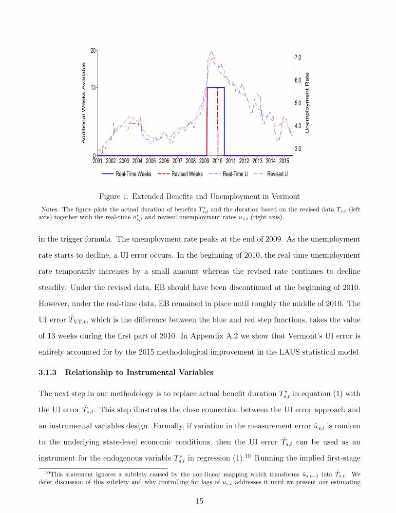
We use the EB program in the state of Vermont to illustrate the two components. Figure

1 plots four lines. The blue solid step function shows the additional weeks of benefits available

to eligible unemployed in Vermont in each calendar week, T ∗VT,t. This series depends on the

most recently reported three month moving-average real-time unemployment rate, plotted by

the dashed blue line. The red dashed step function shows TVT,t, the additional weeks of benefits

that would have been available in Vermont using the revised unemployment rate series plotted

by the dashed red line.

Vermont extended its benefits by an additional 13 weeks in the beginning of 2009. Because

the real-time and the revised unemployment rates move closely together in this period, Vermont

would have triggered an EB extension using either the real-time or the revised data as an input

8States have the option of whether or not to adopt two of the triggers for EB status. We follow the actual statelaws in determining whether to apply the optional triggers. A complication arises with a temporary change in thelaw between December 17, 2010 and December 31, 2013. The EB total unemployment rate trigger requires the(three-month) moving average of the unemployment rate in a state to exceed 110% of its level in the same periodin either of the two previous years. With unemployment in many states still high at the end of 2010 but no longerrising, Congress temporarily allowed states to pass laws extending the lookback period by an additional year. Manystates passed such laws in the week in which the two-year lookback period would have implied an expiration of EB.When we use the revised unemployment rate to construct the duration of benefits under the EB program, we findthat five states would have lost eligibility for EB earlier than in reality. Therefore, in constructing Ts,t, we assumethat states would have adopted the three-year lookback option earlier had the duration of benefits under the EBprogram followed the revised rather than the real-time unemployment rate. Specifically, we set to zero the UI errorfrom the EB program in any week in which a state had not adopted the three-year lookback trigger, the state dideventually adopt the three-year lookback trigger, and the UI error would have been zero had the state adopted thethree-year lookback trigger in that week. This change affects a negligible fraction of observations in our sample (atotal of 20 state-week observations).

9Our algorithm does better than the trigger notices, in the sense that it identifies more than 50 instanceswhere the trigger notices report an incorrect duration or aspect of UI law which we subsequently correct usingcontemporary local media sources, by comparing to the real-time unemployment rate data reported in LAUS pressreleases, or by referencing state legislation. We suspect but cannot confirm that the remaining discrepancies alsoreflect mistakes in the trigger notices. A number of previous papers have relied on information contained in thetrigger notices (Rothstein, 2011; Hagedorn, Karahan, Manovskii, and Mitman, 2015; Hagedorn, Manovskii, andMitman, 2015; Marinescu, 2017). Our investigation reveals that, while small in number, uncorrected mistakes inthe trigger notices could induce some attenuation bias.

14

3.0

4.0

5.0

6.0

7.0

Un

em

plo

ym

en

t R

ate

0

13

20

Ad

ditio

na

l W

ee

ks A

va

ila

ble

2001 2002 2003 2004 2005 2006 2007 2008 2009 2010 2011 2012 2013 2014 2015

Real-Time Weeks Revised Weeks Real-Time U Revised U

Figure 1: Extended Benefits and Unemployment in Vermont

Notes: The figure plots the actual duration of benefits T ∗s,t and the duration based on the revised data Ts,t (leftaxis) together with the real-time u∗s,t and revised unemployment rates us,t (right axis).

in the trigger formula. The unemployment rate peaks at the end of 2009. As the unemployment

rate starts to decline, a UI error occurs. In the beginning of 2010, the real-time unemployment

rate temporarily increases by a small amount whereas the revised rate continues to decline

steadily. Under the revised data, EB should have been discontinued at the beginning of 2010.

However, under the real-time data, EB remained in place until roughly the middle of 2010. The

UI error TVT,t, which is the difference between the blue and red step functions, takes the value

of 13 weeks during the first part of 2010. In Appendix A.2 we show that Vermont’s UI error is

entirely accounted for by the 2015 methodological improvement in the LAUS statistical model.

3.1.3 Relationship to Instrumental Variables

The next step in our methodology is to replace actual benefit duration T ∗s,t in equation (1) with

the UI error Ts,t. This step illustrates the close connection between the UI error approach and

an instrumental variables design. Formally, if variation in the measurement error us,t is random

to the underlying state-level economic conditions, then the UI error Ts,t can be used as an

instrument for the endogenous variable T ∗s,t in regression (1).10 Running the implied first-stage

10This statement ignores a subtlety caused by the non-linear mapping which transforms us,t−1 into Ts,t. Wedefer discussion of this subtlety and why controlling for lags of us,t addresses it until we present our estimating

15

regression T ∗s,t = π0 + π1Ts,t + π2I{t ∈ TEUC02,EUC08} + es,t, where I is an indicator that

controls for the common increase in duration of benefits during the two emergency compensation

periods, we estimate π1 = 1.01 with a standard error of 0.17. Thus, Ts,t and T ∗s,t move one-for-

one. A first stage coefficient of 1 makes the second stage of a two-stage least squares regression

equal to the reduced form regression which replaces T ∗s,t in equation (1) with Ts,t. We impose

this first stage coefficient of 1 and work with the reduced form version because it facilitates our

treatment of the dynamics in the duration of benefits, as we explain next.

3.2 Serial Correlation of Benefit Duration

The UI error Ts,t is a serially correlated process because the underlying measurement error in

unemployment us,t is serially correlated as shown for example in Figure 1 for Vermont.11 When

an outcome variable ys,t+h depends on leads or lags of a persistent right-hand side variable

{Ts,t+j}Jhj=Jl, a regression of ys,t+h only on the contemporaneous Ts,t confounds the response to

Ts,t with the effect of lags and leads of the UI error. In economic terms, labor market outcomes

in some period may depend on both previous UI errors and expected future UI errors.

We follow the macroeconomic approach of plotting impulse responses with respect to struc-

tural innovations to overcome this difficulty.12 Define the current period unexpected component

of the UI error:

εs,t = Ts,t − Et−1Ts,t, (5)

where Et−1Ts,t denotes the expectation of Ts,t using information available until period t−1. We

will estimate the specification:

ys,t+h = β(h)εs,t + Γ(h)Xs,t + νs,t+h, (6)

equation. An approach conceptually similar to ours is to regress T ∗s,t on Ts,t and define Ts,t to be the residuals from

this regression. These residuals display a correlation of 0.99 with our measure of Ts,t obtained as the differencebetween T ∗s,t and Ts,t.

11The persistence in the UI error reflects both the UI law (once triggered onto a tier a state must remain on forat least 13 weeks) and serial correlation in us,t. To give a sense of the latter, the first 8 autocorrelation coefficientsof us,t are 0.78, 0.63, 0.52, 0.45, 0.40, 0.35, 0.32, 0.29.

12Ramey (2016) extensively surveys the use of this approach and Stock and Watson (2017) provide a detailedeconometric treatment. Our implementation follows Romer and Romer (1989) and Jorda (2005) in directly esti-mating the horizon h response to a shock.

16

where ys,t+h is an outcome variable in state s and period t + h, εs,t is the UI error innovation

in state s and period t, and Xs,t is a vector of covariates. Specification (6) deals with the

correlation between Ts,t and past UI errors by replacing it with the serially-uncorrelated innova-

tion εs,t. Thus, the coefficients β(h) = E[ys,t+h|Ts,t = 1, Ts,t−1, Ts,t−2, . . . ,Xs,t]− E[ys,t+h|Ts,t =

0, Ts,t−1, Ts,t−2, . . . ,Xs,t] for h = 0, 1, 2, ... trace out the impulse response function of y with

respect to an unexpected one-month increase in the UI error. For labor market variables, this

response reflects both the direct contemporaneous effect of increased eligibility due to the UI er-

ror and the change in agents’ expectations about future benefit duration. Section 5.1 reports the

persistence of the increase in actual potential benefit duration following a UI error innovation

by setting ys,t+h = Ts,t+h in equation (6). We discuss the effect on expectations in Section 5.2.2.

We implement three methods to identify the unexpected component in the UI error εs,t.

Our preferred approach allows the UI error Ts,t to follow a first-order discrete Markov chain

with probability πT

(Ts,t+1 = xj | Ts,t = xi;us,t, t

)that T transitions from a value xi to a value

xj. A Markov chain is more general than an autoregressive process. Indeed, inspection of

the time series of the UI errors in Figure 1 reveals a stochastic process better described by

occasional discrete jumps than by a smoothly evolving diffusion. The transition probabilities

may depend on the unemployment rate and calendar time because the mapping from a mea-

surement error in the unemployment rate to a UI error depends on whether the measurement

error occurs in a region of the unemployment rate space sufficiently close to a trigger thresh-

old.13 In practice, we aggregate Ts,t up to a monthly frequency and estimate each probability

πT

(Ts,t+1 = xj | Ts,t = xi;us,t, t

)as the fraction of transitions of the UI error from xi to xj

for observations in the same unemployment rate and calendar time bin. We form a vector of

discrete possible values of x from one-half standard deviation wide bins of Ts,t. Finally, once we

have estimated the transition probabilities of the Markov process, we calculate the expectation

Et−1Ts,t and form the UI error innovation εs,t using equation (5).14

13For example, measurement error in the mid-2000s does not cause a UI error for Vermont in Figure 1 becausethe unemployment rate is far below the threshold for triggering an extension of benefits. Conditioning on calendartime reflects the time variation in UI laws and triggers due to enactment of an emergency compensation program.

14A trade-off exists between finer partitioning of the state space and retaining sufficient observations to make

17

In sensitivity exercises we show that our results are robust to two alternative processes for

Ts,t which impose additional structure. First, we obtain the innovations by first-differencing the

UI error, εs,t = Ts,t − Ts,t−1. This transformation is simpler than a first-order discrete Markov

chain but comes at the cost of imposing a martingale structure on the UI error. Second, we

obtain the innovations as the residual from a regression of Ts,t on lags of itself (and Xs,t). This

approach imposes smooth autoregressive dynamics on the process for Ts,t and is equivalent to

estimating impulse responses with respect to Ts,t directly while controlling for lags of the UI

error.15

4 Data and Summary Statistics

We draw on a number of sources to obtain data for state-level outcome variables. From the

BLS, along with the revised unemployment rate, we use monthly payroll employment from the

Current Employment Statistics (CES) program and monthly labor force participation from the

LAUS program. The CES data have the advantage of deriving (after revisions) directly from

administrative tax records. We obtain data on the number of UI payments across all programs

by state and month from the DOL ETA 539 and ETA 5159 activity reports and from special

tabulations for the July 2008 to December 2013 period.16 We obtain monthly data on vacancies

from the Conference Board Help Wanted Print Advertising Index and the Conference Board

Help Wanted Online Index. We use the first for the years 1996-2003 and aggregate local areas up

to the state level. We use the online index for 2007-2015. The print index continues until June

the exercise non-trivial. We estimate separate transition matrices for each of the following sequential groupings,motivated by the divisions shown in Table A.1: December 2008 – May 2012 and 5.5 ≤ us,t < 7; December 2008– May 2012 and 7 ≤ us,t < 8.5; December 2008 – May 2012 and us,t ≥ 8.5; June 2012 – December 2013 and5.5 ≤ us,t < 7; June 2012 – December 2013 and 7 ≤ us,t < 9; June 2012 – December 2013 and us,t ≥ 9; January2002 – December 2003 and us,t ≥ 5.5; us,t ≥ 5.5; us,t < 5.5. We have experimented with coarser groupings and

larger bins of Ts,t with little effect on our results.15This last approach also ensures orthogonality of the innovation to lagged values of Ts,t in a finite sample,

which the general Markov approach does not. We have verified the innovations under the Markov approach haveapproximately zero correlation with lagged values of Ts,t in our sample.

16These are found at http://www.ows.doleta.gov/unemploy/DataDownloads.asp and http:

//workforcesecurity.doleta.gov/unemploy/euc.asp respectively, last accessed February 10, 2016. Thedata report the total number of UI payments each month. To express as a share of the total unemployed, wedivide by the number of unemployed in the (revised) LAUS data and multiply by the ratio 7/[days in month]because the number of unemployed are a stock measure as of the CPS survey reference week.

18

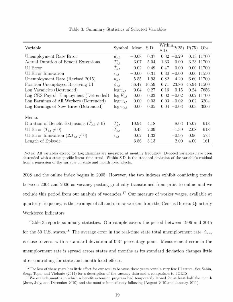
Table 3: Summary Statistics of Selected Variables

Variable Symbol Mean S.D.WithinS.D.

P(25) P(75) Obs.

Unemployment Rate Error us,t −0.08 0.37 0.32 −0.29 0.13 11700Actual Duration of Benefit Extensions T ∗s,t 3.07 5.04 1.33 0.00 3.23 11700

UI Error Ts,t 0.02 0.49 0.47 0.00 0.00 11700UI Error Innovation εs,t −0.00 0.31 0.30 −0.00 0.00 11550Unemployment Rate (Revised 2015) us,t 5.55 1.93 0.82 4.20 6.60 11700Fraction Unemployed Receiving UI φs,t 36.47 16.59 6.71 23.86 45.94 11500Log Vacancies (Detrended) log vs,t 0.04 0.27 0.16 −0.15 0.24 7656Log CES Payroll Employment (Detrended) logEs,t 0.00 0.03 0.02 −0.02 0.02 11700Log Earnings of All Workers (Detrended) logws,t 0.00 0.03 0.03 −0.02 0.02 3204Log Earnings of New Hires (Detrended) logws,t 0.00 0.05 0.04 −0.03 0.03 3066

Memo:

Duration of Benefit Extensions (Ts,t 6= 0) T ∗s,t 10.94 4.18 8.03 15.07 618

UI Error (Ts,t 6= 0) Ts,t 0.43 2.09 −1.39 2.08 618

UI Error Innovation (∆Ts,t 6= 0) εs,t 0.02 1.33 −0.95 0.96 573Length of Episode 3.86 3.13 2.00 4.00 161

Notes: All variables except for Log Earnings are measured at monthly frequency. Denoted variables have beendetrended with a state-specific linear time trend. Within S.D. is the standard deviation of the variable’s residualfrom a regression of the variable on state and month fixed effects.

2008 and the online index begins in 2005. However, the two indexes exhibit conflicting trends

between 2004 and 2006 as vacancy posting gradually transitioned from print to online and we

exclude this period from our analysis of vacancies.17 Our measure of worker wages, available at

quarterly frequency, is the earnings of all and of new workers from the Census Bureau Quarterly

Workforce Indicators.

Table 3 reports summary statistics. Our sample covers the period between 1996 and 2015

for the 50 U.S. states.18 The average error in the real-time state total unemployment rate, us,t,

is close to zero, with a standard deviation of 0.37 percentage point. Measurement error in the

unemployment rate is spread across states and months as its standard deviation changes little

after controlling for state and month fixed effects.

17The loss of these years has little effect for our results because these years contain very few UI errors. See Sahin,Song, Topa, and Violante (2014) for a description of the vacancy data and a comparison to JOLTS.

18We exclude months in which a benefit extension program had temporarily lapsed for at least half the month(June, July, and December 2010) and the months immediately following (August 2010 and January 2011).

19

A potential concern is that there are too few or too small UI errors to identify significant

effects of benefit extensions on macroeconomic outcomes. Table 3 shows that this is not true.

There are 618 cases in which a state would have had a different duration of extensions using

the revised data. Conditional on a UI error occurring, that is Ts,t 6= 0, the standard deviation

of the UI error is larger than 2 months.19 The interquartile range is roughly 3.5 months. The

fact that there is enough variation in the UI error relative to outcome variables such as the

unemployment rate explains the small standard errors of our estimates below.

The average episode of a non-zero UI error lasts nearly 4 months and occurs when benefit

extensions already provide an additional 11 months of UI eligibility. Most of these episodes

occur during the Great Recession. As already discussed in Section 3.2, measurement error in

the unemployment rate u translates into a UI error T only if the state’s unemployment rate is

sufficiently near a trigger threshold. This fact explains why we construct T rather than using

u directly and why the UI errors occur mostly in the Great Recession, a period when both the

EUC program created additional trigger thresholds and most states had unemployment rates

high enough for measurement error in the unemployment rate to translate into a UI error.

5 Labor Market Effects of Benefit Extensions

In this section we present impulse responses of labor market outcomes to UI benefit extensions

triggered purely by measurement error. To review, our basic approach for overcoming the en-

dogeneity of UI benefit extensions to macroeconomic conditions is to isolate the component of

benefit extensions arising from mismeasurement of state unemployment rates in real time, which

we denote by Ts,t, and to construct the unexpected and serially uncorrelated component of the

UI error, εs,t. Motivated by our investigation of the sources of unemployment rate revisions, we

begin our analysis in Section 5.1 under the assumption that the measurement error in the unem-

ployment rate underlying εs,t is random. We discuss the interpretation of the impulse responses

in Section 5.2. Section 5.3 relaxes the assumption that εs,t is random. In Section 5.4 we discuss

19Throughout the paper, when referring to months of benefit extensions we use the convention that one monthequals 4.33 weeks.

20

the possibility of measurement error in the revised unemployment rate and provide auxiliary

evidence that the revised unemployment rate better measures true economic conditions than

the real-time unemployment rate. Finally, Section 5.5 presents additional sensitivity analysis.

5.1 Baseline Results

We measure the responses of labor market variables to a one-month UI error innovation εs,t

using the specification:

ys,t+h = β(h)εs,t +12∑j=1

γj(h)us,t−j + ds(h) + dt(h) + νs,t+h, (7)

where ys,t+h is an outcome variable in state s and period t + h, εs,t is the UI error innovation

in state s and period t, and ds(h) and dt(h) are state and month fixed effects. Including lags

of the unemployment rate as controls approximates the experiment of comparing two states on

similar unemployment paths until one receives an unexpected UI error. These covariates also

directly address the fact that, even when us,t is strictly exogenous, the non-linear mapping from

us,t to Ts,t depends on us,t−1.20 We include state and month fixed effects because they increase

precision by absorbing substantial variation in our main outcome variables.

The coefficients β(h) for h = 0, 1, 2, ... trace out the impulse response function of y with

respect to a one-month unexpected change in the UI error. The identifying assumption that εs,t

is orthogonal to νs,t+h, E[εs,t× νs,t+h|controls] = 0, is valid if the underlying measurement error

in the unemployment rate us,t that gives rise to εs,t is random.

Figure 2 shows impulse responses of the innovation ε and the UI error T to a one-month

20The mapping is easiest to see in a hypothetical example in which a single extension threshold u determinesthe extension of benefits. In this case, a positive UI error, Ts,t = T ∗s,t − Ts,t > 0, is associated with a low revisedunemployment rate, u∗s,t−1 > u > us,t−1, and the opposite for a negative UI error. Controlling for the laggedunemployment rate directly addresses any such correlation. Even without controlling for the lagged unemploymentrate, this correlation would have a minor affect on our estimates. In results available as supplementary material, weuse actual unemployment rate revisions but artificial trigger thresholds to construct artificial UI error series duringthe late 1990s, a period with very few actual UI extensions. We then estimate regressions of us,t on εs,t withoutcontrolling for lags of the unemployment rate. These placebo regressions produce coefficients clustered around zero.Moreover, with multiple thresholds the sign of any correlation is ambiguous. The twelve lags of the unemploymentrate also directly control for the small increment to the variation in the measurement error u accounted for by lagsof the unemployment rate shown in Table A.2. When we plot impulse responses of us,t+h we continue to includeboth the fixed effect and the lagged values of us,t in an OLS framework since the large time series (more than 200monthly observations) exceeds the cross-sectional component (Alvarez and Arellano, 2003).

21

Response of ε

-0.2

0.0

0.2

0.4

0.6

0.8

1.0

1.2

Inno

vatio

n in

UI D

urat

ion

Erro

r

0 1 2 3 4 5 6 7 8

Response of T

-0.2

0.0

0.2

0.4

0.6

0.8

1.0

1.2

Cha

nge

in U

I Dur

atio

n Er

ror

0 1 2 3 4 5 6 7 8

Figure 2: Serial Correlation

Notes: The figure plots the coefficients on εs,t from the regression ys,t+h = β(h)εs,t +∑12j=1 γj(h)us,t−j + ds(h) +

dt(h) + νs,t+h, where ys,t+h = εs,t+h is the UI error innovation (left panel) or ys,t+h = Ts,t+h is the UI error (rightpanel). The dashed lines denote the 90 percent confidence interval based on two-way clustered standard errors.

innovation ε. In all figures, dashed lines report the 90 percent confidence interval based on

standard errors two-way clustered by state and by month. The innovation exhibits essentially

no serial correlation. The lack of serial correlation provides support for our choice of modeling

T as a first-order Markov process.21 The UI error T rises one-for-one with ε on impact and then

decays over the next few months with a half-life of roughly 2 months.

Figure 3 illustrates the main result of the paper. The left panel shows the responses from

regression (7) when the left-hand side variable is the (revised) unemployment rate. The unem-

ployment rate barely responds to the increase in the duration of benefits. The point estimate

for the response is essentially zero. The upper bound is roughly 0.02 percentage point. The

data do not reject a zero response of the unemployment rate at any horizon.22

21Time aggregation from weekly to monthly frequency could explain the small correlation between months t andt+ 1, as an increase in T in week 3 or 4 of month t would produce a positive innovation in both t and t+ 1.

22The small standard errors reflect the substantial variation in the right-hand side variable ε relative to theoutcome variable u shown in Table 3. To get a back-of-the-envelope estimate of the standard error withoutcontrolling for lags of u, consider a bivariate regression with a zero coefficient and no clustering. The standarderror of the coefficient would be 1√

N

σuσε

= 1√11550

0.820.33 ≈ 0.023. This standard error is close to the standard errors

we estimate when we two-way cluster by month and state but do not control for lags of u. Two-way clustering atthe quarter and state level instead of the month and state level to allow for correlation in the residuals across statesand over time has almost no effect on the standard errors shown in Figure 3. For example, the standard error ofthe unemployment rate response at the one month horizon would increase from 0.009 to 0.010 and the standarderror at the four month horizon is identical up to three decimal places.

22

Response of u

Model: UI increases u by 3.1 p.p. in Great Recession

-0.05

0.00

0.05

0.10

0.15

Cha

nge

in U

nem

ploy

men

t Rat

e (P

P)

0 1 2 3 4 5 6 7 8

Response of ln v

Model: UI increases u by 3.1 p.p. in Great Recession

-0.050

-0.025

0.000

0.025

Cha

nge

in L

og V

acan

cies

0 1 2 3 4 5 6 7 8

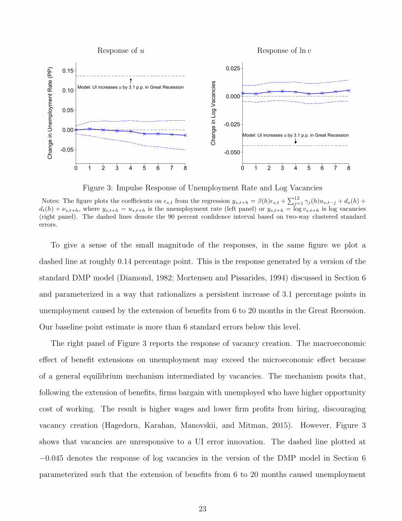
Figure 3: Impulse Response of Unemployment Rate and Log Vacancies

Notes: The figure plots the coefficients on εs,t from the regression ys,t+h = β(h)εs,t +∑12j=1 γj(h)us,t−j + ds(h) +

dt(h) + νs,t+h, where ys,t+h = us,t+h is the unemployment rate (left panel) or ys,t+h = log vs,t+h is log vacancies(right panel). The dashed lines denote the 90 percent confidence interval based on two-way clustered standarderrors.

To give a sense of the small magnitude of the responses, in the same figure we plot a

dashed line at roughly 0.14 percentage point. This is the response generated by a version of the

standard DMP model (Diamond, 1982; Mortensen and Pissarides, 1994) discussed in Section 6

and parameterized in a way that rationalizes a persistent increase of 3.1 percentage points in

unemployment caused by the extension of benefits from 6 to 20 months in the Great Recession.

Our baseline point estimate is more than 6 standard errors below this level.

The right panel of Figure 3 reports the response of vacancy creation. The macroeconomic

effect of benefit extensions on unemployment may exceed the microeconomic effect because

of a general equilibrium mechanism intermediated by vacancies. The mechanism posits that,

following the extension of benefits, firms bargain with unemployed who have higher opportunity

cost of working. The result is higher wages and lower firm profits from hiring, discouraging

vacancy creation (Hagedorn, Karahan, Manovskii, and Mitman, 2015). However, Figure 3

shows that vacancies are unresponsive to a UI error innovation. The dashed line plotted at

−0.045 denotes the response of log vacancies in the version of the DMP model in Section 6

parameterized such that the extension of benefits from 6 to 20 months caused unemployment

23

Response of total φ

-1.0

-0.5

0.0

0.5

1.0

1.5

Cha

nge

in F

ract

ion

Rec

eivi

ng U

I (PP

)

0 1 2 3 4 5 6 7 8

Response of φ by tier

-1.0

-0.5

0.0

0.5

1.0

Cha

nge

in F

ract

ion

Rec

eivi

ng U

I (PP

)

0 1 2 3 4 5 6 7 8

Affected tiersUnaffected tiers

Figure 4: Impulse Response of Fraction Receiving UI

Notes: The figure plots the coefficients on εs,t from the regression φs,t+h = β(h)εs,t +∑12j=1 γj(h)us,t−j + ds(h) +

dt(h) + νs,t+h. In the left panel, φs,t+h includes UI recipients in all tiers. The right panel plots separate impulseresponse functions for UI recipients in tiers with a UI error (solid red line) and in tiers without a UI error (dashedgreen line). In the right panel the sample starts in 2008. The dashed lines denote the 90 percent confidence intervalbased on two-way clustered standard errors.

in the Great Recession to remain persistently high.

Figure 4 demonstrates that the absence of a response of unemployment and vacancies occurs

despite a higher fraction of the unemployed receiving UI benefits following a UI error innovation.

The left panel shows that upon impact, the fraction of unemployed receiving UI benefits increases

by 0.5 percentage point. The fraction remains high for the next two months and then declines

to zero. This response is reasonable. The innovations in the UI error take place when benefits

have, on average, already been extended for roughly 11 months. Using CPS data we estimate

that between 0.5 and 1 percent of unemployed would be affected by such an extension, implying

a take-up rate in the range of estimates documented by Blank and Card (1991). The right

panel of Figure 4 splits the increase in UI receipt into recipients on tiers without a UI error

(dashed green line with triangles) and recipients on tiers affected by the UI error (solid red line

with crosses).23 All of the additional take-up of UI benefits occurs among individuals on tiers

directly affected by the UI error.

23We do not have UI receipt by tier for the EB or TEUC02 programs. Therefore, the sample in the right panelof Figure 4 starts in 2008 and the sum of the two lines in the right panel does not equal the impulse response inthe left panel which is based on the full sample.

24

Table 4: Response of Variables to UI Error Innovation

Levels Differences

Horizon: 1 4 1 4

1. Unemployment rate 0.003 −0.003 0.003 −0.003(0.009) (0.015) (0.009) (0.015)

2. Log Vacancies 0.003 0.004 0.001 0.002(0.004) (0.005) (0.002) (0.003)

3. Fraction Receiving UI 0.751∗∗ −0.039 0.914∗∗ 0.129(0.253) (0.263) (0.291) (0.285)

4. Log CES Payroll Employment 0.000 0.000 0.000 −0.000(0.000) (0.000) (0.000) (0.000)

5. Labor Force Participation Rate 0.001 0.001 0.012+ 0.014(0.018) (0.022) (0.007) (0.014)

6. Log Earnings (All Workers) 0.001 −0.001 0.004 0.002(0.002) (0.002) (0.004) (0.003)

7. Log Earnings (New Hires) −0.000 0.004 −0.000 0.004(0.003) (0.004) (0.004) (0.007)

Notes: Each cell reports the result from a separate regression of the dependent variable indicated in the leftcolumn on the innovation in the UI error εs,t, controlling for state and period fixed effects and 12 monthly or 4quarterly lags of us,t. In the panel headlined “Levels” the dependent variable enters in levels. In the panel headlined“Differences” the dependent variable enters with a difference relative to its value in t− 1 (rows 1, 3, 4, 5) or t− 2(rows 2, 6, 7). Standard errors clustered by state and time period are shown in parentheses. ∗∗ denotes significanceat the 1% level.

Finally, Table 4 summarizes the responses of a number of labor market variables. The left

panel of the table reports the point estimates and standard errors at horizons 1 and 4 for the

variables already plotted along with employment, labor force participation, and worker earnings.

The right panel displays results for a slight modification of our baseline regression (7) in which

we replace the dependent variable with its difference relative to the period before the UI error

innovation occurs. If UI error innovations are uncorrelated with lagged outcome variables, then

including the dependent variable in either levels or differences will yield a similar coefficient.24

24For us,t, the lags of the unemployment rate included in the baseline regression (7) make the differencing withrespect to us,t−1 redundant, but for the other variables we have not imposed a zero effect in t − 1 in the levelsspecification of the left panel Table 4. We prefer the levels specification in the left panel because of a time-aggregation issue. An increase in T in week 4 of month t − 1 that persists through month t would be associatedwith an increase in εs,t and may also be correlated with variables in t− 1. Indeed, we have already noted the smallserial correlation of εs,t due to this time aggregation issue. The attenuation from differencing with respect to t− 1is likely quite small for variables based on the CPS (the unemployment rate and labor force participation rate) orthe CES (payroll employment) which use as a reference period the week or pay period containing the 12th day of

25

Across all variables, we find economically negligible responses to a positive one-month innovation

in the UI error. The standard errors rule out effects much larger in magnitude.

5.2 Interpretation of Responses

Our results provide direct evidence of the limited macroeconomic effects of increasing the du-

ration of unemployment benefits around the neighborhood of a typical UI error, or by about

3 months after a state has already extended benefits by nearly one year. In this section we

discuss the informativeness of this evidence for changes in labor market outcomes in response

to other UI policies such as increasing benefits all the way from 26 to 99 weeks as observed in

some states after the Great Recession.

We start by performing a linear extrapolation and then discuss the merits of this procedure.

Extrapolating linearly the upper bound of a 0.02 percentage point increase in the unemployment

rate with respect to a one-month UI error innovation, we conclude that increasing benefits from

26 to 99 would increase the unemployment rate by roughly 0.02 × 17 ≈ 0.3 percentage point.

Similarly, linearly extrapolating a lower bound of −0.03 percentage point yields a maximum

decrease in the unemployment rate of 0.5 percentage point for an extension of benefits from 26

to 99 weeks.25

These calculations neglect two potentially important differences between the variation un-

derlying our estimated impulse responses and a typical extension of benefits in the aftermath

of the Great Recession. First, the response of labor market outcomes to an extension from a

baseline level of 26 weeks may differ from the response to an extension from a baseline level

of 70 weeks. Second, the UI errors have lower persistence relative to a policy that increases

maximum benefits to 99 weeks as in the Great Recession. We discuss each difference in turn

the month. Likewise, the reference period for the vacancy measure for month t is from mid month in t− 1 to midmonth in month t. However, the problem is larger for the fraction of unemployed who receive UI, which countsall UI payments during the month, and for the wage measures which include total earnings over the month. Weaccount for this issue in Table 4 by taking a difference of these variables with respect to their t− 2 value.

25The lower bound encompasses the estimates of Di Maggio and Kermani (2015) who find a UI output multiplierof 1.9. To compare to Di Maggio and Kermani (2015), note that total EB and EUC payments between 2009 and2013 were $50.5 billion, $79.2 billion, $58.7 billion, $39.7 billion, and $22.0 billion. Applying a multiplier of 1.9 tothe peak amount of $79.2 billion in 2010 gives an increase in output in 2010 of 1.0% of GDP. An application ofOkun’s law yields a 0.3-0.5 percentage point decline in the unemployment rate in that year.

26

Table 5: Baseline Duration and Length of Episode

Dependent variable: Unemployment rate Log vacancies Fraction receiving

Horizon: 1 4 1 4 1 4Panel A:

εs,t 0.004 −0.003 0.002 0.007 0.925∗∗ −0.051(0.010) (0.018) (0.008) (0.010) (0.249) (0.280)

εs,t × [Ts,t > 10.5] −0.002 0.000 0.003 −0.006 −0.425 0.028(0.008) (0.019) (0.011) (0.012) (0.395) (0.297)

Panel B:

εs,t 0.008 0.008 0.002 0.004 0.596∗ −0.345(0.011) (0.019) (0.005) (0.006) (0.257) (0.226)

εs,t × [Lengths,t > 6] −0.020 −0.042 0.003 −0.001 0.584 1.149∗

(0.012) (0.027) (0.012) (0.013) (0.472) (0.569)Observations 10,850 10,700 7,084 6,932 10,750 10,600

Notes: Each column of each panel reports the coefficients from a separate regression. All regressions control forstate and month fixed effects and 12 lags of us,t. In panel A, the UI error innovation εs,t is interacted with whetherbenefit duration without the error exceeds 10.5 months. In panel B, the UI error innovation εs,t is interacted withwhether the length of the episode during which the UI error remains non-zero exceeds 6 months. Standard errorstwoway-clustered by state and month and are in parentheses. ∗∗,∗ denote significance at the 1% and 5% levels.

and argue neither appears especially important in practice.

5.2.1 Baseline Level of Benefit Duration

The typical UI error in our sample causes an increase in the maximum potential duration

of benefits starting from a baseline level of roughly 16.5 months.26 A concern for the linear

extrapolation that we performed may be that labor market variables respond more to benefit

extensions occurring around a lower baseline level of duration, as these extensions directly affect

the eligibility of a larger fraction of unemployed.

Panel A of Table 5 assesses this possibility by allowing the effect of a UI innovation εs,t in

26The variation in the duration of benefits around a baseline level well beyond the 6 months of regular benefitsis typical of studies based on cross-state variation. The reason is that cross-state variation in benefit durationconcentrates in recessions when the first tier of emergency compensation uniformly increases benefit duration acrossall states and many states qualify for multiple additional tiers. For example, Hagedorn, Karahan, Manovskii, andMitman (2015) study county border pairs where the potential duration of benefits differs across the two counties.We calculate that the median maximum duration is roughly 16.5 months for the border county with the lowerduration in the pair, exactly the same as in our study.

27

regression (7) to vary depending on the baseline level of duration of benefits. Specifically, the

table reports the effects on unemployment, vacancies, and claimants of a UI error innovation

interacted with whether the extension of benefits occurs when the duration of extended benefits

is above 10.5 months (so the duration of total benefits is above the median of 16.5 months).

The first four columns show that the effect of a UI error innovation on the unemployment rate

and vacancies does not vary significantly with the baseline duration of extensions. Column (5)

shows a larger point estimate for the fraction of unemployed claiming UI in response to a UI

error innovation when the baseline duration is lower, consistent with an extension from a lower

baseline level directly affecting a larger fraction of unemployed persons (however, this interaction

is not statistically significant). The small response of unemployment and vacancies to a UI error

even at low baseline levels of duration supports the plausibility of a linear extrapolation.

5.2.2 Persistence

The typical extension of benefits is more persistent than a typical UI error in our sample.27

Let us start with a discussion of why this difference might not matter. The fraction of the

unemployed who become immediately eligible for benefits does not depend on the persistence

of the extension. Therefore, whether a benefit extension arises due to a UI error or not only

affects the immediate response of unemployment and vacancies insofar as workers and firms have

different expectations of future benefit eligibility depending on the source of the extension. While

we do not have direct evidence on this point, it seems unlikely that agents could distinguish in

real-time between an increase due to the UI error component Ts,t and an increase due to the

component Ts,t, because doing so would require agents to know in real-time the unemployment

rate error made by the BLS. If agents do not distinguish the source of a change in benefit

extension duration, then the impact response of labor market variables to a UI error equals

27The duration of a typical benefit extension in our data has a half-life of 12.5 months as opposed a half-lifeof roughly 2.5 months for a typical UI error. While the extensions above 26 weeks around the Great Recessionlasted for 5 years, no state experienced a benefit extension to the maximum of 99 weeks for the whole of the EUCprogram. Rather, adjustments to the EUC law frequently changed the maximum potential duration across statesand changes in unemployment caused states to trigger off and on tiers. Moreover, the temporary nature of theauthorization for the EUC program meant that during the Great Recession the average time remaining until theprogram’s expiration was roughly 5 months.

28

the response to a typical extension of benefits even though realized subsequent extensions may

differ.28 In Section 6 we use the structure of the DMP model to show that the responses we

estimated with respect to a one-month UI innovation imply limited macroeconomic effects of

benefit extensions even when agents perceive a benefit extension caused by a UI error to be

more transitory than a benefit extension caused by the increase in unemployment.

We next demonstrate that the magnitude of the responses of unemployment and vacancies

does not depend significantly on the length of the UI error episode. While this type of evidence

does not allow us to directly infer agents’ expectations about the persistence of the UI errors,

the stability of responses across different realized lengths of UI error spells is reassuring for the

plausibility of a linear extrapolation. Panel B of Table 5 reports coefficients from interacting the

UI innovation εs,t in our baseline regression (7) with an episode length of greater than 6 months,

where an episode means the length of time a UI error remains non-zero. The median episode

of longer than 6 months lasts a total of 11 months. The first two sets of columns show that

unemployment and vacancies do not respond differentially during episodes of length greater

than 6 months. The small response of unemployment and vacancies to UI errors of greater

lengths again enhance the plausibility of a linear extrapolation. The third set of columns shows

that the fraction of unemployed who are receiving benefits does increase in the length of the

episode and especially at longer horizons. This difference is expected because, by construction,

an episode of longer than 6 months has a direct effect on eligibility at the 4 month horizon

whereas an episode shorter than 6 months might not.

5.3 Robustness to Process for us,t

In Section 3.1.1, we distinguished among three sources of revisions to the state unemployment

rate. One of these, the use of a state space smoother in the revision process, makes the revised

28Related to this point, the UI literature contains conflicting evidence on how forward-looking are potentialunemployment benefit recipients with respect to future benefit eligibility. Card and Levine (2000) and Card,Chetty, and Weber (2007) estimate a small decline in exit hazard for regular benefit recipients when a benefitextension occurs. Johnston and Mas (Forthcoming) find evidence of a decline in exit hazard for recipients far fromthe benefit extension but no effect on the behavior of recipients within 30 weeks of the extension. Ganong andNoel (2017) find a large decline in consumption when exhaustion occurs, suggesting agents do not anticipate theexhaustion.

29

unemployment rate in each month dependent on the full available time series of the input

variables at the point of revision. This dependence raises a concern that the unemployment

rate revision in month t partly depends on realizations of variables after month t. Importantly

for our empirical design, we found that this source of revisions contributes little to the variation

in us,t and hence εs,t. Nonetheless, we now implement two alternative strategies which remain

valid even if the BLS revisions process induces a correlation between us,t and the future path

of variables.

5.3.1 Controlling for us,t

We augment our baseline specification to:

ys,t+h = β(h)εs,t + g ({us,t}) +12∑j=1

γj(h)us,t−j + ds(h) + dt(h) + νs,t+h, (8)

where the flexible function g(.) may allow for leads, lags, and non-linear transformations of the

measurement error in the unemployment rate us,t. Specification (8) controls directly for any

correlation between functions of us,t and the future path of ys,t+h which may arise from the

revision process.

To build intuition for specification (8), it helps to start with the case where ys,t+h = us,t+h

and g(.) = ρ(h)us,t−1. Recalling that εs,t depends on data in period t− 1 due to reporting lags,

us,t−1 controls for the measurement error in the unemployment rate during the same month

as the data which determine εs,t. The term ρ(h)us,t−1, therefore, partials out any “normal”

covariation between us,t−1 and us,t+h which might result from the revision process. The iden-

tification exploits the fact that the mapping between us,t−1 and Ts,t is not strictly monotonic;

there are many instances of measurement error in the unemployment rate which do not give

rise to a UI error, as illustrated in Figure 1 in the case of Vermont. Formally, the identifi-

cation assumption becomes E[εs,t × νs,t+h|Xs,t, us,t−1] = 0. A sufficient condition for this to

hold is that any correlation between the unemployment rate measurement error us,t−1 and the

future path of unemployment does not change if us,t−1 causes a UI error, except through the

direct response of future variables to the UI error. That is, E[us,t+h|Xs,t, us,t−1, εs,t = ε] =

30

Response of u

-0.05

0.00

0.05

0.10

0.15

Cha

nge

in U

nem

ploy

men

t Rat

e (P

P)

0 1 2 3 4 5 6 7 8

Response of φ

-1.0

-0.5

0.0

0.5

1.0

Cha

nge

in F

ract

ion

Rec

eivi

ng U

I (PP

)

0 1 2 3 4 5 6 7 8

Figure 5: Impulse Responses Controlling for Measurement Error us,t

Notes: The figure plots the coefficients on εs,t from the regression ys,t+h = β(h)εs,t+ρ(h)us,t−1+∑12j=1 γj(h)us,t−j+

ds(h) + dt(h) + νs,t+h, where ys,th = us,t+h is the unemployment rate (left panel) or ys,th = φs,t+h is the fractionof unemployed receiving UI on all tiers (right panel). The dashed lines denote the 90 percent confidence intervalbased on two-way clustered standard errors.

E[us,t+h|Xs,t, us,t−1, εs,t = 0] + β(h)ε = Γ(h)Xs,t + ρ(h)us,t−1 + β(h)ε. Including leads, lags, or

non-linear transformations of us,t−1 in the function g(.) allows for the baseline correlation of

us,t−1 and us,t+h to vary with the level or path of us,t.

We begin in Figure 5 by reporting the impulse response functions for the unemployment

rate us,t and the total fraction receiving benefits φs,t based on specification (8) with only us,t−1

added to the regression. Both impulse response functions appear nearly identical to those

without the measurement error in the unemployment rate control. Specifically, the response of

unemployment to a positive one-month UI error innovation is essentially zero while the fraction

of unemployed receiving UI increases by roughly 0.5 percentage point.

We next allow for more flexible functions of the measurement error in the unemployment

rate to enter into the specification. Table 6 reports the one and four month responses of the

unemployment rate, log vacancies, and the fraction of unemployed receiving UI. Each cell of the

table reports the coefficient or standard error on the UI error innovation εs,t from a separate

regression of the dependent variable in the column header on the UI error innovation, the

baseline controls of twelve lags of the unemployment rate and state and month fixed effects,

31

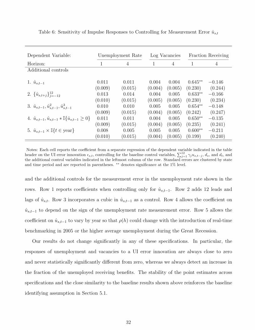
Table 6: Sensitivity of Impulse Responses to Controlling for Measurement Error us,t

Dependent Variable: Unemployment Rate Log Vacancies Fraction Receiving

Horizon: 1 4 1 4 1 4Additional controls

1. us,t−1 0.011 0.011 0.004 0.004 0.645∗∗ −0.146(0.009) (0.015) (0.004) (0.005) (0.230) (0.244)

2. {us,t+j}12j=−12 0.013 0.014 0.004 0.005 0.633∗∗ −0.166(0.010) (0.015) (0.005) (0.005) (0.230) (0.234)

3. us,t−1, u2s,t−1, u

3s,t−1 0.010 0.010 0.005 0.005 0.654∗∗ −0.148

(0.009) (0.015) (0.004) (0.005) (0.242) (0.247)4. us,t−1, us,t−1 ∗ I{us,t−1 ≥ 0} 0.011 0.011 0.004 0.005 0.650∗∗ −0.135

(0.009) (0.015) (0.004) (0.005) (0.235) (0.241)5. us,t−1 × I{t ∈ year} 0.008 0.005 0.005 0.005 0.600∗∗ −0.211

(0.010) (0.015) (0.004) (0.005) (0.199) (0.240)

Notes: Each cell reports the coefficient from a separate regression of the dependent variable indicated in the tableheader on the UI error innovation εs,t, controlling for the baseline control variables,

∑12j=1 γjus,t−j , ds, and dt, and

the additional control variables indicated in the leftmost column of the row. Standard errors are clustered by stateand time period and are reported in parentheses. ∗∗ denotes significance at the 1% level.

and the additional controls for the measurement error in the unemployment rate shown in the

rows. Row 1 reports coefficients when controlling only for us,t−1. Row 2 adds 12 leads and

lags of us,t. Row 3 incorporates a cubic in us,t−1 as a control. Row 4 allows the coefficient on

us,t−1 to depend on the sign of the unemployment rate measurement error. Row 5 allows the

coefficient on us,t−1 to vary by year so that ρ(h) could change with the introduction of real-time

benchmarking in 2005 or the higher average unemployment during the Great Recession.

Our results do not change significantly in any of these specifications. In particular, the

responses of unemployment and vacancies to a UI error innovation are always close to zero

and never statistically significantly different from zero, whereas we always detect an increase in

the fraction of the unemployed receiving benefits. The stability of the point estimates across

specifications and the close similarity to the baseline results shown above reinforces the baseline

identifying assumption in Section 5.1.

32

5.3.2 Alternative Series for Ts,t

Our second approach is to construct an alternative series for Ts,t which does not depend at

all on the BLS unemployment rate revision process. Instead, we exploit CPS sampling error

and generate an alternative unemployment rate series to proxy for the true unemployment

rate us,t. Specifically, sampling error in the CPS contributes to a wedge between the insured

unemployment rate in administrative records and the insured unemployment rate calculated

from the CPS based on the number of CPS respondents reporting unemployment duration of

less than 26 weeks and job loss as the reason for unemployment. Thus, we can infer CPS

sampling error from the gap between these two measures and remove this sampling error to

obtain an alternative proxy for us,t. In practice, we regress the BLS real-time unemployment

rate u∗s,t on the contemporaneous and 12 lags of the administrative insured unemployment rate

and the labor force share of unemployed ineligible for regular UI taken directly from the CPS

(i.e. duration greater than 26 weeks or not job-loser), as well as state and month fixed effects.

The R2 of this regression is 0.96. We use the fitted value of this regression instead of the revised

unemployment rate to proxy for us,t. We then construct the UI error Ts,t = T ∗s,t−Ts,t, where in

Ts,t we use the new us,t as the input into the mapping fs,t(.), and extract the innovations εs,t

from the newly constructed UI error.

We estimate impulse responses using the specification (7) but with our alternative series

for the UI error innovation εs,t. Relative to the baseline results, the implementation here more

tightly restricts the variation in UI duration to coming from a particular source of error in the

real-time unemployment rate. By construction, the UI error and the underlying measurement

error in the unemployment rate now do not depend on the subsequent path of variables. Figure 6

reports the impulse response functions for the unemployment rate and the total fraction receiving

benefits based on the alternative series for the UI errors. Once again, both impulse response

functions are quite similar to those reported above. The response of unemployment to a positive

one-month UI error innovation is statistically indistinguishable from zero while the fraction of

unemployed receiving UI increases by roughly 0.8 percentage point.

33

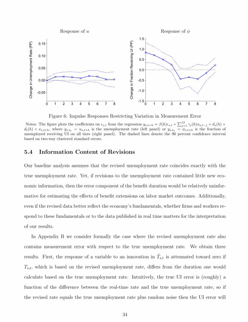
Response of u

-0.05

0.00

0.05

0.10

0.15

Cha

nge

in U

nem

ploy

men

t Rat

e (P

P)

0 1 2 3 4 5 6 7 8

Response of φ

-1.5

-1.0

-0.5

0.0

0.5

1.0

1.5

Cha

nge

in F

ract

ion

Rec

eivi

ng U

I (PP

)

0 1 2 3 4 5 6 7 8

Figure 6: Impulse Responses Restricting Variation in Measurement Error

Notes: The figure plots the coefficients on εs,t from the regression ys,t+h = β(h)εs,t +∑12j=1 γj(h)us,t−j + ds(h) +

dt(h) + νs,t+h, where ys,th = us,t+h is the unemployment rate (left panel) or ys,th = φs,t+h is the fraction ofunemployed receiving UI on all tiers (right panel). The dashed lines denote the 90 percent confidence intervalbased on two-way clustered standard errors.

5.4 Information Content of Revisions

Our baseline analysis assumes that the revised unemployment rate coincides exactly with the

true unemployment rate. Yet, if revisions to the unemployment rate contained little new eco-

nomic information, then the error component of the benefit duration would be relatively uninfor-

mative for estimating the effects of benefit extensions on labor market outcomes. Additionally,

even if the revised data better reflect the economy’s fundamentals, whether firms and workers re-

spond to these fundamentals or to the data published in real time matters for the interpretation

of our results.

In Appendix B we consider formally the case where the revised unemployment rate also

contains measurement error with respect to the true unemployment rate. We obtain three

results. First, the response of a variable to an innovation in Ts,t is attenuated toward zero if

Ts,t, which is based on the revised unemployment rate, differs from the duration one would

calculate based on the true unemployment rate. Intuitively, the true UI error is (roughly) a

function of the difference between the real-time rate and the true unemployment rate, so if

the revised rate equals the true unemployment rate plus random noise then the UI error will

34

inherit that noise. Second, the size of the attenuation bias is decreasing in the variance share

of the innovation εs,t generated by true UI errors rather than measurement error in the revised

unemployment rate. Third, if the revised unemployment rate is at least as good a measure of

the true unemployment rate as the real-time rate, then the bias is bounded above by a factor

of 2.

The remainder of this section substantiates the informativeness of the revisions and argues

that the revised unemployment rate better measures the true economic fundamental than the

real-time rate. We have already presented two types of evidence consistent with the data

revisions containing new information. First, Section 3.1.1 and Appendix A.2 described the new

source data and methodological improvements incorporated in the revisions process. Second,

we would not have obtained the economically significant response of the fraction of unemployed

receiving benefits if the revised data added only noise to the real-time estimates.

We now show that the revised unemployment rate better correlates with actual consumer

spending. We estimate a horse-race specification:

ys,t = βrevisedureviseds,t−2 + βreal-timeureal-times,t−2 + νs,t, (9)

where ys,t denotes either new auto registrations (from R.L. Polk) or new building permits

(from the Census Bureau). Both series reflect spending done by a state’s residents, derive from

actual registration data, and have no mechanical correlation with either the real-time or the

revised unemployment rate. We interpret the coefficients βrevised and βreal-time as the weights

one should assign to the revised and real-time unemployment rates as statistical predictors

of spending behavior. The unemployment rates enter the regression with a two-month lag to

reflect the timing of the release of the LAUS state unemployment data, which usually occurs

for month t− 1 around the 20th day of month t. Therefore, agents at the beginning of month

t have access to the real-time unemployment rate for month t− 2 but not for month t− 1 or t.

Agents do not know the revised unemployment rate for t− 2 at the start of month t, but may

respond to the economy’s true fundamentals. Under the maintained assumption that higher

unemployment is associated with lower spending, a finding of βrevised < 0 and βreal-time = 0

35

Table 7: Spending Decisions and Unemployment Data

Dependent Variable

Auto Sales Building Permits

(1) (2) (3) (4) (5) (6)

Revised URs,t−2 −0.42∗∗ −0.52∗∗ −0.09∗∗ −0.10∗∗

(0.11) (0.13) (0.02) (0.02)Real-time URs,t−2 −0.34∗∗ 0.09+ −0.07∗∗ 0.01

(0.10) (0.05) (0.02) (0.02)State FE Yes Yes Yes Yes Yes YesTime FE Yes Yes Yes Yes Yes YesDep. var. mean 5.4 5.4 5.4 0.5 0.5 0.5Dep. var. sd 2.0 2.0 2.0 0.4 0.4 0.4R2 0.61 0.61 0.61 0.73 0.76 0.77Observations 10,096 9,847 9,847 15,800 12,147 12,147

Notes: The dependent variable is indicated in the table header. The auto sales data come from R.L. Polk andcorrespond to the state of residency of the purchaser. The permits data are for new private housing units and comefrom the Census Bureau. Standard errors are clustered by state and month and denoted in parentheses. ∗∗,∗ ,+

denote significance at the 1%, 5%, and 10% level.

provides support for the joint hypothesis that revised data improve the quality of measurement

of economic fundamentals and that agents in real time base their decisions on these fundamentals

and ignore the measurement error.

Table 7 reports the results. Columns (1), (2), (4), and (5) show that both the revised and

the real-time unemployment rates are negatively correlated with spending. The key results

are shown in columns (3) and (6) in which we introduce jointly both variables in regression

(9). For both auto sales and building permits, we estimate βrevised < 0 and βreal-time ≈ 0.

The estimates of βrevised are close in magnitude to the estimates in columns (1) and (4) which

exclude the real-time rate. Thus, the revised unemployment rate contains all the information

about spending patterns and, given knowledge of both series, one should put essentially no

weight on the real-time data to predict actual spending.

Survey responses from the Michigan Survey of Consumers (MSC) provide further evidence

that the revised unemployment data contains significant new information. The MSC asks 500

36

respondents each month a series of questions covering their own financial situation and their

views on the economy. For survey months in or after the year 2000, the Michigan Survey

Research Center allowed us to merge external state-level data to anonymized responses. Because

sample sizes are too small to aggregate to the state-month level, we instead run our horse-race

regression at the individual level and cluster standard errors by state and by month:

yi,s,t = βrevisedureviseds,t + βreal-timeureal-times,t + ΓXi,s,t + νi,s,t. (10)

Table 8 reports results for a subset of questions in the survey that we expect to correlate with

the local unemployment rate. For brevity, we report only specifications with both unemploy-

ment rates. Averaging across the eight outcomes we consider, the first column shows that a

higher revised unemployment rate is associated with worse subjective perceptions of economic

conditions. It also shows that, conditional on the revised unemployment rate, the real-time

unemployment rate appears to add no information. This result repeats in various individual

outcomes as shown in columns (2) to (9).

To summarize, the results in Tables 7 and 8 provide direct additional evidence that the

revised data better align with true economic fundamentals than the real-time data. Therefore,

the conservative upper bound for the possible attenuation bias derived in Appendix B holds.

Applying this upper bound to the confidence interval upper bound of a 0.02 percentage point

increase in the unemployment rate in response to a one-month UI error yields a maximum

response of 0.04 percentage point.

5.5 Further Robustness

In this section we investigate the robustness of our main findings along various other dimensions.

Table 9 compares the one and four month responses of the unemployment rate, log vacancies,

and the fraction of unemployed receiving UI in the baseline specification to the responses in

alternative specifications. The first row of the table repeats the baseline results from Section 5.1.

Rows 2 and 3 assess the practical importance of controlling for lags of the unemployment

rate. In row 2, we additionally control non-parametrically for the lagged unemployment rate

37

Table 8: Beliefs and Unemployment Data

Dependent Variable

AVG PJOB PEXP PINC2 INEX DUR CAR BUS12 BUS5

(1) (2) (3) (4) (5) (6) (7) (8) (9)

Revised URs,t−2 0.028+ 0.663∗ 0.012 −1.086∗ −0.186 0.043∗ 0.025 0.007 0.004(0.015) (0.310) (0.016) (0.476) (0.224) (0.021) (0.018) (0.034) (0.027)

Real-time URs,t−2 −0.015 −0.472 −0.006 0.477 0.042 −0.025 −0.016 0.005 −0.007(0.011) (0.310) (0.012) (0.403) (0.197) (0.018) (0.015) (0.027) (0.021)

State FE Yes Yes Yes Yes Yes Yes Yes Yes YesTime FE Yes Yes Yes Yes Yes Yes Yes Yes YesWeighted Yes Yes Yes Yes Yes Yes Yes Yes YesIndividual controls Yes Yes Yes Yes Yes Yes Yes Yes YesDep. var. mean -0.01 18.82 2.61 46.02 3.31 2.08 2.22 3.18 3.14Dep. var. sd 1.00 25.16 1.31 36.95 16.50 1.73 1.81 1.92 1.79R2 0.16 0.47 0.83 0.71 0.14 0.64 0.64 0.78 0.79Observations 82,291 81,719 80,529 70,036 79,425 78,631 78,626 75,571 79,123

Notes: The dependent variable is indicated in the table header. AVG: simple mean of normalized variables withhigher values denoting worse subjective expectations. PJOB: chance will lose job in 5 years. PEXP: personalfinances b/w next year (1: Will be better off. 3: Same. 5: Will be worse off). PINC2: percent chance of incomeincrease. INEX: family income expectations 1 year recoded. DUR: durables buying attitudes (1: Good. 3: Pro-con.5: Bad). CAR: vehicle buying attitudes (1: Good. 3: Pro-con. 5: Bad). BUS12: economy good/bad next year (1:Good times. 2: Good with qualifications. 3: Pro-con. 4: Bad with qualifications. 5: Bad times). BUS5: economygood/bad next 5 years (1: Good times. 2: Good with qualifications. 3: Pro-con. 4: Bad with qualifications.5: Bad times). Individual controls: sex, marital status, age, age2, age3, four educational attainment categories,and log income, each interacted with month. Regressions are weighted using survey weights. Standard errors areclustered by state and month and denoted in parentheses. ∗,+ denote significance at the 5% and 10% level.

by partitioning the lagged unemployment rate into 0.5 percentage point wide bins and adding

indicator variables for whether the lagged rate lies in each bin. Row 3 removes the lags of the

unemployment rate from the baseline specification. In all cases, we obtain very similar results

to the baseline. Row 4 removes the lags of the unemployment rate and the state ds and month

dt fixed effects from the specification (so there are no controls). We again find similar point

estimates. However, the standard errors more than double in row 3 with no controls because

fixed effects absorb a large fraction of the variation in outcome variables unrelated to the UI

error innovation.

Next, we assess the robustness of our results to the assumed process for the UI errors used in

38

Table 9: Sensitivity of Impulse Responses to Alternative Specifications

Dependent Variable: Unemployment Log FractionRate Vacancies Receiving

Horizon: 1 4 1 4 1 4Regressor Controls

1. εs,t {us,t−j}12j=1, ds, dt 0.003 −0.003 0.003 0.004 0.751∗∗−0.039(0.009) (0.015) (0.004) (0.005) (0.253) (0.263)

2. εs,t {us,t−j}12j=1, ds, dt, uIs,t−1 0.003 −0.003 0.003 0.004 0.758∗∗−0.033

(0.009) (0.015) (0.004) (0.005) (0.244) (0.245)3. εs,t ds, dt −0.014 −0.023 0.006 0.007 0.684∗∗−0.137

(0.025) (0.026) (0.005) (0.006) (0.235) (0.235)4. εs,t None −0.003 −0.029 0.015 0.019+ 0.548 −0.478

(0.078) (0.077) (0.009) (0.011) (0.664) (0.702)

5. ∆Ts,t {us,t−j}12j=1, ds, dt 0.004 0.004 −0.000 −0.001 0.556∗∗ 0.081(0.008) (0.012) (0.003) (0.003) (0.133) (0.187)

6. Ts,t {Ts,t−j, us,t−j}12j=1, ds, dt 0.002 −0.003 −0.001 −0.001 0.911∗∗ 0.012(0.008) (0.014) (0.005) (0.005) (0.266) (0.242)

7. ∆T ∗s,t ∆Ts,t, {us,t−j}12j=1, ds, dt 0.006 0.011 −0.003 −0.003 1.018∗∗ 0.369+

(0.007) (0.012) (0.003) (0.004) (0.178) (0.193)

Notes: Each cell reports the coefficient from a separate regression of the dependent variable indicated in the tableheader on the right-hand side variable indicated in the leftmost column of the row, controlling for the variablesindicated in the second column of the row. Standard errors are clustered by state and time period and are reportedin parentheses. ∗∗,+ denote significance at the 1% and 10% level.

extracting the innovations. To account for the sparsity and non-linearity of the UI error process,

our preferred approach imposes a first-order Markov process that generalizes the autoregressive

persistence usually imposed on macroeconomic data. In row 5, we instead simply first difference

the UI error and replace εs,t in equation (7) with ∆Ts,t = Ts,t − Ts,t−1. In row 6, we report

the coefficient on the level of Ts,t but controlling for twelve lags of Ts,t. This specification is

conceptually similar to defining the UI error innovation as the structural residual from a vector

autoregression in Ts,t and us,t with twelve lags and Ts,t first in a Cholesky ordering.29 The

29Formally, after demeaning with respect to the state and month fixed effects, the specification is a Jorda(2005) local projection based on a bivariate system in us,t and Ts,t with twelve lags and Ts,t being first in the

Cholesky ordering. The Cholesky identification assumption is that the forecast error in Ts,t does not respond tothe contemporaneous structural innovation to the unemployment rate. As a justification for the ordering, recallthat due to reporting lags UI benefits in month t are only a function of unemployment rates for month t − 1 andearlier.

39

limited response of unemployment and vacancies and the significantly positive response of the

fraction receiving UI remain robust to these alternative specifications.

Finally, the last row of Table 9 shows a control function specification in which we regress

outcomes ys,t+h on the change in the observed UI duration ∆T ∗s,t controlling for the change in

the UI duration ∆Ts,t based on the revised data, the lags of unemployment, state dummies,

and monthly dummies.30 Because we control for changes in UI duration due to fundamentals

with ∆Ts,t, the remaining variation in ∆T ∗s,t reflects changes in UI benefit duration that arises

from measurement error only. As the last row shows, the effects of unemployment and vacancies

remain small and statistically insignificant whereas the response of the fraction of unemployed

receiving UI increases slightly.

6 DMP Model with Benefit Extensions

Our empirical estimates suggest a small macroeconomic effect of extending benefits. In this

section we interpret these results through the lens of a standard DMP model (Diamond, 1982;

Mortensen and Pissarides, 1994). The model illustrates the basic logic of why benefit extensions

might lead to higher unemployment. We use it to assess the sensitivity of our conclusions when

workers and firms perceive a UI error to be more transitory than a benefit extension caused

by a persistent increase in the unemployment rate and to extensions which persist for longer

than a year as in the aftermath of the Great Recession. Additionally, we show that in the

model the extension of benefits from 26 to 99 weeks does not introduce a significant degree of

non-linearity, corroborating the results in Section 5.2.1 for the stability of the responses of labor

market variables to UI errors at different baseline levels of duration.

We augment a standard DMP model with a UI policy. The model shares many features

with the models used by Hagedorn, Karahan, Manovskii, and Mitman (2015) and Mitman and

Rabinovich (2014) to argue that benefit extensions cause unemployment to remain persistently

high following a negative shock. We reach a different conclusion because our empirical estimates

30We thank an anonymous referee for suggesting the similarity of our approach to a control function approach.

40

imply a lower level of the opportunity cost of employment in the model than assumed by these

papers.31 We describe here only the elements of the model essential to our argument and provide

additional detail in Appendix C.

Each period a measure ut of unemployed search for jobs and a measure 1− ut of employed

produce output. Unemployed individuals find jobs at a rate ft which is determined in equi-

librium. Employed individuals separate from their jobs at an exogenous rate δt. Employed

individuals who lose their jobs become eligible for UI benefits with probability γ. Unemployed

who are eligible for UI and do not find jobs lose their eligibility with probability et. The key

policy variable in our model is the (expected) duration of benefits T ∗t which equals the inverse

of the expiration probability, T ∗t = 1/et. Ineligible unemployed who do not find jobs remain

ineligible for UI benefits.

Risk-neutral individuals discount the future with a factor β. Employed individuals consume

their wage earnings wt. The value of an individual who begins period t as employed is given by

Wt. Ineligible unemployed derive a flow value from non-market work equal to ξ. The value of

an individual who begins period t as ineligible is U It . Eligible unemployed additionally receive

a UI benefit B. The value of an individual who begins period t as eligible is UEt . We define the

value of the average unemployed individual as Ut = ωtUEt + (1−ωt)U I

t , where ωt is the fraction

of unemployed who are eligible for and receive UI.

The surplus of employment for the average unemployed is given by the difference between the

value of working and the value of unemployment, St = Wt−Ut = wt− zt+β(1− δt− ft)EtSt+1,

where zt denotes the flow opportunity cost of employment for the average unemployed:

zt = ξ + ωtB − (δt(γ − ωt) + (1− ft)ωtet) β(EtUE

t+1 − EtU It+1

)︸ ︷︷ ︸bt

, (11)

In equation (11), ξ denotes the flow value of non-market work and bt denotes the benefit compo-

nent of the opportunity cost of employment. This expression nests the corresponding expression

for the opportunity cost in the standard DMP model (for instance, Shimer, 2005) where bt = B

31This result echoes Costain and Reiter (2008), who point out that models with a high level of opportunity costgenerate stronger effects of policies on labor market outcomes than the effects found in cross-country comparisons.

41

if et = 0 and γ = ωt = 1, that is when all unemployed receive benefits. More generally, bt is

lower than the benefit B. The difference occurs because some unemployed are not eligible for

benefits and, even for those unemployed who are eligible, benefits eventually expire.32 Extend-

ing benefits, which here means a decline in the expiration probability et, increases the fraction

of unemployed who are eligible ωt and raises bt and zt.

The value of a firm which has matched with a worker is given by Jt = pt−wt+β(1−δt)EtJt+1,

where pt denotes aggregate labor productivity. Free entry drives the expected value of creating

a vacancy to zero, giving κqt

= βEtJt+1, where κ denotes the upfront cost that an entrant

pays to create a vacancy and qt denotes the rate at which vacancies are filled. A constant

returns to scale matching technology mt = mt(ut, vt) converts job seekers and vacancies into

new matches. Denoting market tightness by θt = vt/ut, an unemployed matches with a firm at

rate ft(θt) = mt/ut and firms fill vacancies at rate qt(θt) = mt/vt = ft(θt)/θt.

Firms and workers split the surplus from an additional match according to the generalized

Nash bargaining solution. We denote by µ the bargaining power of workers. The wage is chosen

to maximize the product Sµt J1−µt . This leads to a standard wage equation:

wt = µpt + (1− µ)zt + µκθt. (12)

The duration of UI benefits is given by T ∗t = Tt + Tt, where Tt denotes the duration of UI

benefits in the absence of any measurement error and Tt is the UI error. Consistent with the

results in Section 5.4 that agents respond only to the revised unemployment rate, we assume

that firms and workers know the underlying fundamentals (for instance, ut, pt, wt etc.) at the

beginning of each period. The statistical agency makes errors in the measurement of the true

unemployment rate which result in UI errors Tt. Thus, agents distinguish in real time between

extensions caused by UI errors and extensions caused by true fundamentals.

We now discuss the effects of UI policy in this model. An increase in the current duration of

benefits affects equilibrium outcomes to the extent that firms and workers expect it to persist

32The first effect is captured by the first term of bt which is lower than B when ωt < 1. The second effect iscaptured by the second term which is positive because γ > ωt and EtUEt+1 > EtU It+1.

42

in future periods. Combining the definition of firm’s value Jt with the free entry condition, the

decision to create a vacancy in the current period depends on the expectation of the present

discounted value of firm profits:

κ

qt(θt)= Et

∞∑j=1

βj

(j∏i=1

(1− δt+i−1)(1− δt)

)(pt+j − wt+j) , (13)

where qt(θt) is a decreasing function of current market tightness θt = vt/ut. By raising the frac-

tion of unemployed who are eligible for UI, an extension of benefits increases future opportunity

costs and wages as shown in equation (12). Higher wages lower the expected present value of

firm profits and decrease firms’ willingness to create vacancies. Fewer vacancies make it more

difficult for the unemployed to find jobs, increasing the unemployment rate.33

We parameterize two versions of the model (see Appendix C for more details). In the “low

b” model we pick b = 0.06 and z = ξ + b = 0.87 in the steady state of the model. The value of

b = 0.06 accords with the finding in Chodorow-Reich and Karabarbounis (2016) that benefits

comprise a small fraction of the average opportunity cost. In the “high b” model we pick b = 0.15

and z = ξ + b = 0.96. The value of z = 0.96 was chosen by Hagedorn and Manovskii (2008) to

target the sensitivity of wages with respect to productivity in the aggregate data.

Figure 7 plots the impulse of the unemployment rate with respect to a one-month UI er-

ror innovation using model-simulated data. As described above, an extension of UI benefits

reduces firm profits from filling a vacancy. In the high b model, firm profits are very small on

average because average match surplus – the difference between the marginal product and the

opportunity cost of employment – is small. Therefore, the extension of benefits lowers firms’

willingness to create vacancies substantially. As the left panel of Figure 7 shows, the maximal

response of the unemployment rate is close to 0.14 percentage point in the high b model. In

the low b model depicted in the right panel, the unemployment rate increases by less than 0.02

percentage point. With a low b, firm profits are on average higher and the extension of benefits

33In our model all workers have the same job-finding rate irrespective of UI eligibility, a point we return to inthe conclusion. Allowing UI policy to affect worker search intensity in this model would further discourage vacancycreation by reducing the job-filling rate as well as directly increase unemployment by lowering the match rate fora given number of vacancies and unemployed.

43

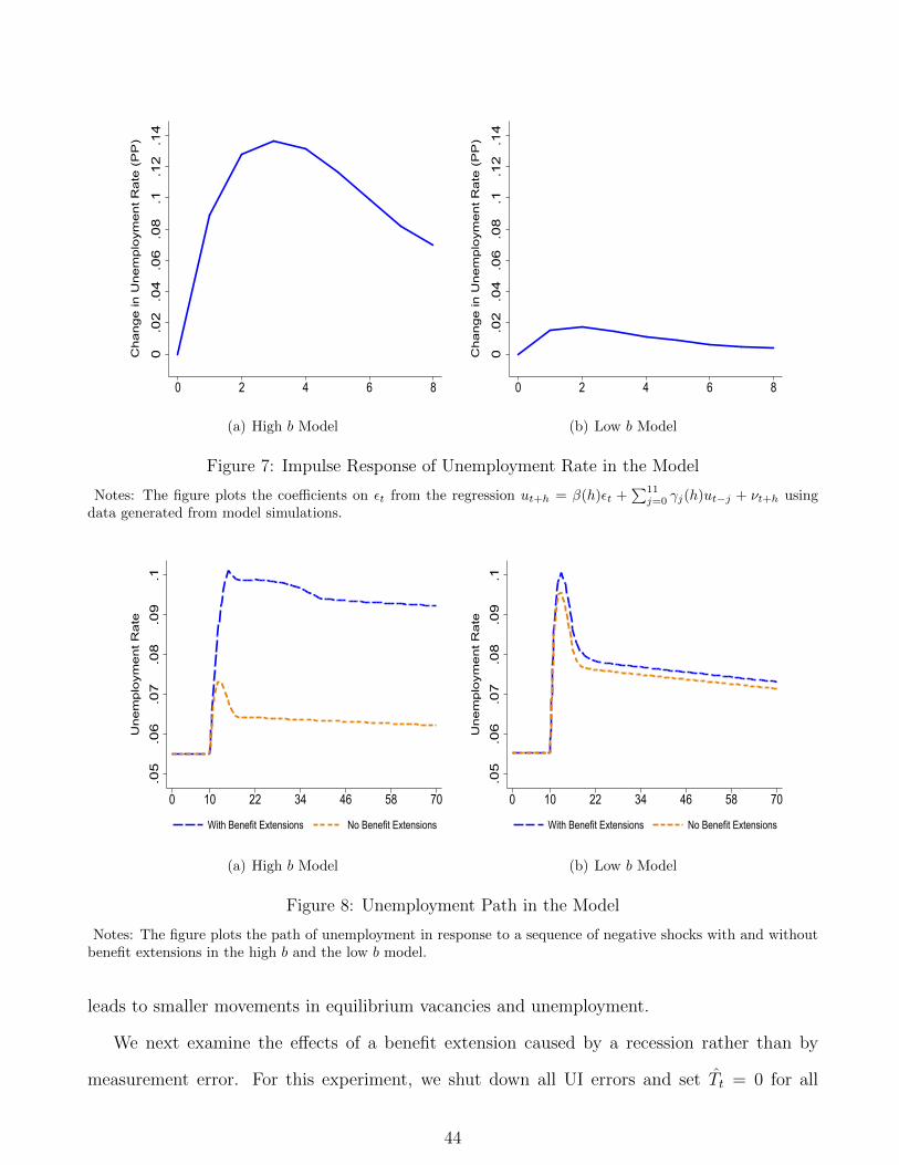
0.0

2.0

4.0

6.0

8.1

.12

.14

Ch

an

ge

in U

ne

mp

loym

en

t R

ate

(P

P)

0 2 4 6 8

(a) High b Model

0.0

2.0

4.0

6.0

8.1

.12

.14

Ch

an

ge

in U

ne

mp

loym

en

t R

ate

(P

P)

0 2 4 6 8

(b) Low b Model

Figure 7: Impulse Response of Unemployment Rate in the Model

Notes: The figure plots the coefficients on εt from the regression ut+h = β(h)εt +∑11j=0 γj(h)ut−j + νt+h using

data generated from model simulations.

.05

.06

.07

.08

.09

.1U

ne

mp

loym

en

t R

ate

0 10 22 34 46 58 70

With Benefit Extensions No Benefit Extensions

(a) High b Model

.05

.06

.07

.08

.09

.1U

ne

mp

loym

en

t R

ate

0 10 22 34 46 58 70

With Benefit Extensions No Benefit Extensions

(b) Low b Model

Figure 8: Unemployment Path in the Model

Notes: The figure plots the path of unemployment in response to a sequence of negative shocks with and withoutbenefit extensions in the high b and the low b model.

leads to smaller movements in equilibrium vacancies and unemployment.

We next examine the effects of a benefit extension caused by a recession rather than by

measurement error. For this experiment, we shut down all UI errors and set Tt = 0 for all

44

periods. We start each of the low b and high b economies in a stochastic steady state in which

no shock occurs for a large number of periods. Beginning in month 10, we introduce a sequence

of productivity and separation shocks chosen so that unemployment reaches roughly 10 percent

with benefit extensions turned on. Appendix C reports the paths of these shocks.

The left panel of Figure 8 plots the paths of unemployment in the high b model with and

without a benefit extension policy. The upper line shows the path when benefit extensions

follow a policy rule similar to that in place during the Great Recession, so that the duration of

benefits rises from 6 to eventually 20 months. Unemployment peaks at roughly 10 percent and

remains persistently high. The lower line shows the path of unemployment in an alternative

UI policy regime where the duration of benefits always equals T ∗t = Tt = 6 months. Consistent

with the conclusions of Mitman and Rabinovich (2014) and Hagedorn, Karahan, Manovskii,

and Mitman (2015), the difference between the two lines shows the large effect that benefit

extensions have on the path of the unemployment rate in the DMP model with a high b.

By contrast, the right panel of Figure 8 shows a much smaller effect of benefit extensions on

unemployment dynamics. As in the high b model, the duration of benefits increases to 20 months

as soon as the unemployment rate exceeds 9 percent. However, the level of the opportunity cost

is small on average and, therefore, this extension does not affect significantly the path of the

unemployment rate. The average distance between the two unemployment paths is less than

0.3 percentage point, close to the linear extrapolation in Section 5.2. Because only the low b

model matches the response of unemployment to a one-month UI error innovation, the results

in Figure 8 validate the limited influence of UI extensions in a DMP model with large and

persistent benefit extensions.

7 Conclusion

Identifying the effect of UI benefit extensions on macroeconomic outcomes is challenging be-

cause benefits are extended in times of elevated unemployment. This simultaneity happens both

because U.S. law makes benefit extensions a function of state economic conditions and because

45

policymakers enact emergency compensation in recessions. We show how to use data revisions

to decompose variation in the duration of benefits over time and across states into the part

coming from actual differences in economic fundamentals and the part coming from measure-

ment error in the real-time data used to determine benefit extensions. This methodology is

potentially applicable to other policy variables which depend on measured economic conditions,

other outcome variables, or in different countries.34

Using only the measurement error component for identification, we find an economically rea-

sonable increase in the number of individuals receiving UI, but only a limited influence of benefit

extensions on key state-level macroeconomic outcomes including unemployment, employment,

vacancies, and wages. Our results imply that the unprecedented increase in benefits during the

Great Recession contributed at most 0.3 percentage point to the increase in the unemployment

rate.

A standard DMP model can rationalize this small response if the opportunity cost of giving

up benefits is low for the average unemployed. Other economic channels which may also explain

the limited influence of benefit extensions we measure in the data include an offsetting stimulus

effect from transferring resources to unemployed individuals with high marginal propensity to

consume, labor market spillovers as lower search effort by UI recipients raises job finding rates

for non-recipients, and wage bargaining protocols that do not depend on the opportunity cost

of employment. Quantifying each of these channels separately would be a valuable step for

future research. On the other hand, we know of no labor market theory in which UI extensions

substantially raise unemployment without requiring a high opportunity cost of giving up benefits

and a much larger response of unemployment to a UI error than we measure in the data.

In this paper we do not estimate how individual-level outcomes respond to benefit extensions.

Recent studies have found mixed effects at the individual level (Rothstein, 2011; Farber and

Valletta, 2015; Johnston and Mas, Forthcoming). Can one reconcile the small macroeconomic

34For example, states with high unemployment rates can receive waivers for the cap on the number of monthsan able-bodied adult without benefits can receive SNAP benefits (food stamps) in the United States and manycountries extend UI benefits based on regional unemployment rates.

46

effects we find with those studies which find larger microeconomic effects such as Johnston and

Mas (Forthcoming)? Models with job rationing provide one such avenue. In these models,

the job finding rate of UI recipients declines, giving large microeconomic effect, but the job

finding rate of non recipients increases due to the declining competition in the job market. Such

displacement effects are consistent with the findings of Crepon, Duflo, Gurgand, Rathelot, and

Zamora (2013) and Lalive, Landais, and Zweimuller (2015) among others.

Finally, the microeconomic function of UI is to provide income replacement for individuals

who have lost their jobs. The value of this insurance mechanism may increase in the duration

of an unemployment spell as individuals draw down on their assets and other sources of income.

The results in this paper do not speak to this income support function nor to the microeconomic

rationale for increasing insurance during recessions when the typical duration of unemployment

spells rises. Our results simply say that UI extensions do not have large negative macroeconomic

effects.

References

Alvarez, J., and M. Arellano (2003): “The Time Series and Cross-Section Asymptotics of

Dynamic Panel Data Estimators,” Econometrica, 71(4), 1121–59.

Amaral, P., and J. Ice (2014): “Reassessing the Effects of Extending Unemployment Insur-

ance Benefits,” Federal Reserve Bank of Cleveland, Economic Commentary.

Baily, N. (1978): “Some Aspects of Optimal Unemployment Insurance,” Journal of Public

Economics, 10, 379–402.

Barro, R. (2010): “The Folly of Subsidizing Unemployment,” The Wall Street Journal, August

30.

Blank, R., and D. Card (1991): “Recent Trends in Insured and Uninsured Unemployment:

Is There an Explanation?,” Quarterly Journal of Economics, 106(4), 1157–89.

Boone, C., A. Dube, L. Goodman, and E. Kaplan (2016): “Unemployment Insurance

Generosity and Aggregate Employment,” IZA Discussion Paper No. 10439.

Bureau of Labor Statistics (2014): “Report on Revision to State and Area Time-Series

Models,” Technical Report.

47

(2015): “Questions and Answers on the Local Area Unemployment Statistics (LAUS)

Program 2015 Redesign,” Technical Report.

Card, D., R. Chetty, and A. Weber (2007): “Cash-on-Hand and Competing Models of

Intertemporal Behavior: New Evidence from the Labor Market*,” The Quarterly Journal of

Economics, 122(4), 1511–1560.

Card, D., and P. B. Levine (2000): “Extended benefits and the duration of UI spells:

evidence from the New Jersey extended benefit program,” Journal of Public Economics, 78(1),

107 – 138, Proceedings of the Trans Atlantic Public Economics Seminar on.

Chetty, R. (2006): “A General Formula for the Optimal Level of Social Insurance,” Journal

of Public Economics, 90(10-11), 1879–901.

Chodorow-Reich, G., and L. Karabarbounis (2016): “The Cyclicality of the Opportunity

Cost of Employment,” Journal of Political Economy, 124(6), 1563–618.

Congressional Budget Office (2012): “Unemployment Insurance in the Wake of the

Recent Recession,” Technical Report.

Costain, J., and M. Reiter (2008): “Business Cycles, Unemployment Insurance, and the

Calibration of Matching Models,” Journal of Economic Dynamics and Control, 32, 1120–55.

Crepon, B., E. Duflo, M. Gurgand, R. Rathelot, and P. Zamora (2013): “Do

Labor Market Policies Have Displacement Effects? Evidence from a Clustered Randomized

Experiment,” Quartely Journal of Economics, 128(2), 531–80.

Department of Labor (2015): Chronology of Federal Unemployment Compensation Laws.

Di Maggio, M., and A. Kermani (2015): “The Importance of Unemployment Insurance as

an Automatic Stabilizer,” Columbia Business School Research Paper No. 15-31.

Diamond, P. (1982): “Wage Determination and Efficiency in Search Equilibrium,” Review of

Economic Studies, 49(2), 217–27.

Dieterle, S., O. Bartalotti, and Q. Brummet (2016): “Revisiting the Effects of Unem-

ployment Insurance Extensions on Unemployment: A Measurement Error-Corrected Regres-

sion Discontinuity Approach,” CARRA Working Paper Series No. 2016-01.

Farber, H., and R. Valletta (2015): “Do Extended Unemployment Benefits Lengthen

Unemployment Spells? Evidence from Recent Cycles in the U.S. Labor Market,” Journal of

Human Resources, 50(4), 873–909.

Ganong, P., and P. Noel (2017): “Consumer Spending During Unemployment: Positive

and Normative Implications,” .

48

Hagedorn, M., F. Karahan, I. Manovskii, and K. Mitman (2015): “Unemployment

Benefits and Unemployment in the Great Recession: The Role of Macro Effects,” NBER

Working Paper No. 19499.

Hagedorn, M., and I. Manovskii (2008): “The Cyclical Behavior of Equilibrium Unem-

ployment and Vacancies Revisited,” American Economic Review, 98(4), 1692–706.

Hagedorn, M., I. Manovskii, and K. Mitman (2015): “The Impact of Unemployment

Benefit Extensions on Employment: The 2014 Employment Miracle?,” NBER Working Paper

No. 20884.

Hall, R. (2013): “Some Observations on Hagedorn, Karahan, Manovskii, and Mitman,” Stan-

ford University Working Paper.

Hall, R., and A. Mueller (2015): “Wage Dispersion and Search Behavior,” Stanford Uni-

versity Working Paper.

Hansen, G., and A. Imrohoroglu (1992): “The Role of Unemployment Insurance in an

Economy with Liquidity Constraints and Moral Hazard,” Journal of Political Economy,

100(1), 118–42.

Hornstein, A., P. Krusell, and G. Violante (2011): “Frictional Wage Dispersion in

Search Models: A Quantitative Assessment,” American Economic Review, 101(7), 2873–98.

Johnston, A., and A. Mas (Forthcoming): “Potential Unemployment Insurance Duration

and Labor Supply: The Individual and Market-level Response to a Benefit Cut,” Journal of

Political Economy.

Jorda, O. (2005): “Estimation and Inference of Impulse Responses by Local Projections,”

American Economic Review, 95(1), 161–82.

Kekre, R. (2016): “Unemployment Insurance in Macroeconomic Stabilization,” Harvard Uni-

versity Working Paper.

Kroft, K., and M. Notowidigdo (2015): “Should Unemployment Insurance Vary With the

Unemployment Rate? Theory and Evidence,” Review of Economic Studies, Forthcoming.

Krueger, A., and B. Meyer (2002): “Labor Supply Effects of Social Insurance,” in Handbook

of Public Economics, ed. by A. Auerbach, and M. Feldstein, pp. 2327–92. Elsevier.

Krusell, P., T. Mukoyama, and A. Sahin (2010): “Labour-Market Matching with Precau-

tionary Savings and Aggregate Fluctuations,” Review of Economic Studies, 77(4), 1477–507.

Lalive, R., C. Landais, and J. Zweimuller (2015): “Market Externalities of Large Un-

employment Insurance Extension Programs,” American Economic Review, 105(12), 3564–96.

49

Landais, C., P. Michaillat, and E. Saez (2015): “A Macroeconomic Approach to Optimal

Unemployment Insurance: Theory,” University of California at Berkeley Working Paper.

Levine, P. B. (1993): “Spillover Effects Between the Insured and Uninsured Unemployed,”

Industrial and Labor Relations Review, 47(1), 73–86.

Marinescu, I. (2017): “The General Equilibrium Impacts of Unemployment Insurance: Evi-

dence from a Large Online Job Board,” Journal of Public Economics, 150, 14–29.

Mitman, K., and S. Rabinovich (2014): “Do Unemployment Benefit Extensions Explain

the Emergence of Jobless Recoveries?,” Stockholm University Working Paper.

Mortensen, D., and C. Pissarides (1994): “Job Creation and Job Destruction in the

Theory of Unemployment,” Review of Economic Studies, 61(3), 397–415.

Nakajima, M. (2012): “A Quantitative Analysis of Unemployment Benefit Extensions,” Jour-

nal of Monetary Economics, 59, 686–702.

Pfeffermann, D., and R. Tiller (1996): “Small-Area Estimation with State-Space Mod-

els Subject to Benchmark Constraints,” Journal of the American Statistical Association,

101(476), 1387–97.

Ramey, V. (2016): “Macroeconomic Shocks and Their Propagation,” Handbook of Macroeco-

nomics, 2, 71–162.

Romer, C. D., and D. H. Romer (1989): “Does Monetary Policy Matter? A New Test in the

Spirit of Friedman and Schwartz,” in NBER Macroeconomics Annual, ed. by O. J. Blanchard,

and S. Fischer, vol. 4, pp. 121–184. MIT Press.

Rothstein, J. (2011): “Unemployment Insurance and Job Search in the Great Recession,”

Brookings Papers on Economic Activity, 143–214.

Sahin, A., J. Song, G. Topa, and G. L. Violante (2014): “Mismatch Unemployment,”

American Economic Review, 104(11), 3529–64.

Schmieder, J., T. von Wachter, and S. Bender (2012): “The Effects of Extended Un-

employment Insurance Over the Business Cycle: Evidence from Regression Discontinuity

Estimates over Twenty Years,” Quarterly Journal of Economics, 127(2), 701–52.

Shimer, R. (2005): “The Cyclical Behavior of Equilibrium Unemployment and Vacancies,”

American Economic Review, 95(1), 25–49.

Stock, J., and M. Watson (2017): “Identification and Estimation of Dynamic Causal Effects

in Macroeconomics,” .

50

Summers, L. (2010): “The Economic Case for Extending Unemployment Insurance,” The

White House Blog, July 14.

Tiller, R. (1992): “Time Series Modeling of Sample Survey Data from the U.S. Current

Population Survey,” Journal of Official Statistics, 8(2), 149–66.

51

The Limited Macroeconomic Effects of

Unemployment Benefit Extensions

Online Appendix

Gabriel Chodorow-Reich John Coglianese Loukas Karabarbounis

March 2018

A Data Appendix

In this data appendix we describe the extended benefits programs and the BLS methodology

to estimate the state unemployment rates.

A.1 Extended Benefits and Emergency Compensation Programs

In Table A.1 we list the full set of benefit extension programs, tiers, and triggers in operation

during our sample.

A.2 State Unemployment Rate Estimation Methodology

We outline the BLS methodology for estimating the state unemployment rates. The BLS first

introduced state space models in 1989 and began to apply these models to all states in 1996.

Bureau of Labor Statistics (2014) provides an in-depth but non-technical overview of what

follows and Tiller (1992) and Pfeffermann and Tiller (1996) provide a more technical treatment.

The first step of the real-time estimation involves estimating the state space models sepa-

rately for total unemployment and employment. The unemployment rate is constructed from

these two estimates. Let ys,t + os,t denote the direct count of a variable such as state employ-

ment or unemployment from the CPS, where os,t denotes any outlier component identified using

intervention model methods. For each state, the observation equation is:

ys,t = αs,txs,t + Ls,t + Ss,t + es,t, (A.1)

where xs,t is an external regressor (insured unemployment for unemployment and CES payroll

employment for employment), Ls,t is a trend level, Ss,t is a seasonal component, and es,t is the

1

Tab

leA

.1:

Exte

nded

Ben

efit

and

Em

erge

ncy

Com

pen

sati

onP

rogr

ams,

1996

-201

5

Pro

gram

Tie

rW

eeks

Per

iod

Tri

gger

sE

B1

1309

/25/

1982

-.IU

R≥

5,IU

R≥

1.2*

[(IU

R(y

ear

ago)

+IU

R(2

year

sag

o))/

2]O

RIU

R≥

6O

RT

UR≥

6.5

and

TU

R≥

1.1∗

max{T

UR

(yea

rag

o),T

UR

(2ye

ars

ago)}

EB

27

03/0

7/19

93-.

TU

R≥

8an

dT

UR≥

1.1∗

max{T

UR

(yea

rag

o),T

UR

(2ye

ars

ago)}

EB

1,2

n.a

.12

/17/

2010

-12/

31/2

013

Rep

lace

wit

hm

ax{T

UR

(yea

rag

o),T

UR

(2ye

ars

ago)

,TU

R(3

year

sag

o)}

inE

BT

ier

1T

rigg

er3

and

EB

Tie

r2

Tri

gger

1T

EU

C1

1303

/09/

2002

-12/

31/2

003

Ava

ilab

lein

all

stat

esT

EU

C2

1303

/09/

2002

-12/

31/2

003

Eligi

ble

for

EB

orw

ould

be

elig

ible

ifE

BT

ier

1T

rigg

er1

cuto

fffo

rIU

Rw

ere

4in

stea

dof

5E

UC

113

06/3

0/20

08-1

1/20

/200

8A

vailab

lein

all

stat

esE

UC

120

11/2

1/20

08-0

9/01

/201

2A

vailab

lein

all

stat

esE

UC

114

09/0

2/20

12-1

2/31

/201

3A

vailab

lein

all

stat

esE

UC

213

11/2

1/20

08-1

1/05

/200

9E

ligi

ble

for

EB

OR

IUR≥

4O

RT

UR≥

6E

UC

214

11/0

6/20

09-0

5/31

/201

2A

vailab

lein

all

stat

esE

UC

214

06/0

1/20

12-1

2/31

/201

3T

UR≥

6E

UC

313

11/0

6/20

09-0

5/31

/201

2IU

R≥

4O

RT

UR≥

6E

UC

313

06/0

1/20

12-0

9/01

/201

2IU

R≥

4O

RT

UR≥

7E

UC

39

09/0

2/20

12-1

2/31

/201

3IU

R≥

4O

RT

UR≥

7E

UC

46

11/0

6/20

09-0

5/31

/201

2IU

R≥

6O

RT

UR≥

8.5

EU

C4

606

/01/

2012

-09/

01/2

012

IUR≥

6O

RT

UR≥

9E

UC

410

09/0

2/20

12-1

2/31

/201

3IU

R≥

6O

RT

UR≥

9

Not

es:

Tri

gger

sw

ritt

enin

ital

ics

are

opti

onal

.IU

Ris

the

aver

age

of

the

insu

red

un

emp

loym

ent

rate

inth

eth

irte

enw

eeks

end

ing

two

wee

ks

bef

ore

the

wee

kof

the

trig

ger

not

ice.

TU

Ris

the

aver

age

ofth

eto

tal

un

emp

loym

ent

rate

inth

eth

ree

month

sen

din

gw

ith

the

last

month

of

data

rep

ort

edas

of

the

thir

dF

rid

ayb

efor

eth

eS

un

day

star

tin

gth

ew

eek

ofth

etr

igger

noti

ce.

All

pro

gra

ms

an

dti

ers

ob

eya

thir

teen

wee

kru

lew

her

eby

on

cetr

igger

edon

ati

era

stat

ere

mai

ns

onth

atti

erfo

rat

leas

tth

irte

enw

eeks

(barr

ing

any

chan

ges

inla

w),

an

don

cetr

igger

edoff

ati

erth

est

ate

rem

ain

soff

for

at

least

thir

teen

wee

ks.

Th

eti

me

per

iods

rep

orte

dex

clu

de

ph

ase-

outs

.E

BT

ier

1T

rigger

3b

ecam

eop

erati

on

al

on

03/07/1993.

Au

thori

zati

on

of

the

TE

UC

pro

gra

ms

lap

sed

tem

por

aril

yb

etw

een

01/0

1/20

03an

d01/

07/2

003.

Au

thori

zati

on

of

the

EU

Cp

rogra

ms

lap

sed

tem

pora

rily

bet

wee

n04/04/2010

an

d04/14/2010,

bet

wee

n05

/30/

2010

and

07/2

1/20

10,

and

bet

wee

n11

/28/

2010

an

d12/16/2010.

Bet

wee

n02/22/2012

an

d05/31/20

12

indiv

idu

als

cou

ldre

ceiv

eu

pto

16

wee

ks

of

EU

CT

ier

4b

enefi

tsif

thei

rst

ate

was

not

inan

EB

per

iod

.T

he

main

sou

rce

for

this

tab

leis

Dep

art

men

tof

Lab

or

(2015).

2

observation error. The state space model employment or unemployment is Ys,t = αs,txs,t+Ls,t+

Ss,t = ys,t − es,t.

The model state equations are:

αs,t = αs,t−1 + ηα,s,t, (A.2)

Ls,t = Ls,t−1 +Rs,t + ηL,s,t, (A.3)

Rs,t = Rs,t−1 + ηR,s,t, (A.4)

Ss,t =6∑j=1

Sj,s,t, (A.5)

where es,t, ηα,s,t, ηL,s,t, and ηR,s,t are independent normal random variables, and Sj,s,t are

seasonal frequency functions. A generalized Kalman filter estimates the system.1

BLS introduced a major update in 2005 with the incorporation of real-time benchmarking

to Census Division and national totals. Each month, after estimation of the state space system,

BLS would allocate the residual between the sum of model estimates of not seasonally adjusted

series for Census Divisions (Lt + It) and the national CPS total pro rata to each division, and

then repeat the process for states within a division.2 In that way, the real-time sum of state

employment and unemployment would always equal the national total. However, the pro rata

allocation meant that state-specific residuals would “spillover” to neighboring states. In 2010,

BLS began applying a one-sided moving average Henderson filter to the benchmarked series.

The most recent major update to the real-time model occurred in 2015 and involved three

main changes. First, the benchmarking constraint now enters directly into the state space

filter. The observation vector is augmented to include the difference between the sum of not

seasonally adjusted model state unemployment and employment levels and their Census Division

direct estimate (excluding identified outliers), and the estimation constrains the variance of the

innovation in this component to be zero. Incorporating benchmarking within the state space

1Because of the rotating panel structure of the CPS sample, the observation equation errors may be seriallycorrelated. The generalized Kalman filter uses GLS instead of OLS to find the conditional mean of the state vectorgiven the updated observation vector.

2At the Census Division level the state space estimation excludes the external regressors insured unemploymentor payroll employment. In terms of equations (A.1) to (A.5), αcd,t = 0 and var(ηcd,t) = 0.

3

filter more efficiently allocates the benchmark residual across states. Second, outlier components

os,t identified by intervention model methods are added back to the states from which they

originated after the state space estimation. Both of these changes reduce spillovers of unusual

residuals across states within a division. Third, the 2015 redesign incorporated an improved

seasonal adjustment procedure.

Table A.2 provides an overview of the importance of different components of the revision

process using as a metric theR2 from a regression of us,t on the components.3 The first row shows

that the revisions to the CES employment data explain a small part of the unemployment rate

revision. While the CES revisions themselves can be large, they enter into the unemployment

rate only through the denominator and therefore have a smaller effect on the unemployment rate

revision. The second row adds elements related to the 2015 LAUS redesign and the treatment

of state-specific outliers in the CPS. Specifically, we add to the regression the difference between

the vintage 2014 and vintage 2015 LAUS seasonally adjusted unemployment rates, the difference

between the unemployment rate constructed directly from the CPS monthly files and the real-

time LAUS seasonally unadjusted unemployment rate, the difference between the unemployment

rate constructed directly from the CPS files and seasonally adjusted using an X-11 moving

average and the average of the same variable for three months before and three months after

the observation, and the labor force weighted average of the previous variable for other states in

the same Census Division. These variables increase the explained part of us,t to 49%. In row 3,

adding the component due to updated seasonal factors in the revised data further increases the

explained part of us,t to 59%. Rows 4 and 5 next add lags and leads of us,t to explore whether

the path of the unemployment rate affects the revision through the state space smoother and

symmetric filter. In row 4, adding 12 lags of the unemployment rate raises the R2 by 0.02, while

in row 5 adding the contemporaneous and 12 leads of the unemployment rate raises it by an

additional 0.01.4 Overall, these components explain 62% of the variation in the unemployment

3Because the procedure for the real-time data changed in 2005 and most of the UI errors in our sample occurduring the Great Recession, we limit the sample in this table to 2005 to 2013.

4The incremental R2 is not invariant to the ordering of variables. Including just the 12 lags of the unemploymentrate produces an R2 of 0.10. Adding the contemporaneous and 12 leads raises the R2 to 0.15.

4

Table A.2: Determinants of Unemployment Rate Errors

Determinants R2

CES revisions 0.03+ 2015 LAUS redesign and identification of outliers 0.49+ Updated seasonal factors 0.59+ 12 lags of unemployment rate 0.61+ Contemporaneous and 12 leads of unemployment rate 0.62

Notes: The table reports the R2 from a regression of the measurement error in the unemployment rate us,t onthe regressors indicated in the left column. The sample is January 2005 to December 2013. In the first row, CESrevisions are the log difference between the real-time and revised nonfarm seasonally unadjusted employment levelfrom the CES. The second row adds the difference between the vintage 2014 and vintage 2015 LAUS seasonallyadjusted unemployment rates, the difference between the unemployment rate constructed directly from the CPSmonthly files and the real-time LAUS seasonally unadjusted unemployment rate, the difference between the un-employment rate constructed directly from the CPS files and seasonally adjusted using an X-11 moving averageand the average of the same variable for three months before and three months after the observation, and thelabor force weighted average of the previous variable for other states in the same Census Division. The third rowadds the difference between the revised LAUS seasonally adjusted unemployment rate and the real-time seasonallyunadjusted unemployment rate after rescaling the numerator and denominator by the revised seasonal factors forLAUS unemployment and employment. The fourth row adds 12 lags of the revised unemployment rate. The fifthrow adds the contemporaneous and 12 leads of the revised unemployment rate.

rate revision. Because the LAUS process uses a nonlinear state space model, we would not

expect a linear projection on the major sources of revisions to generate an R2 of 1.

Figure A.1 illustrates that in our example of Vermont the 2015 LAUS technical improvements

account for all of the unemployment rate error during the period of the UI error in the beginning

of 2010.

B Measurement Error in the Revised Data

In this appendix we examine the case in which the revised data measure the fundamentals

with some error. Measurement error in the revised data introduces an attenuation bias in

our estimated impulse responses. We derive an upper bound of this bias under the plausible

assumption that the revised data measure fundamentals with less error than the real-time data.

Even under this upper bound, we can reject the hypothesis that our estimated responses are

consistent with large effects of UI benefit extensions on unemployment.

5

2014 vintage

3.0

4.0

5.0

6.0

7.0

Un

em

plo

ym

en

t R

ate

0

13

20

Ad

ditio

na

l W

ee

ks A

va

ila

ble

2001 2002 2003 2004 2005 2006 2007 2008 2009 2010 2011 2012 2013 2014 2015

Real-Time Weeks Revised Weeks Real-Time U Revised U

Figure A.1: Extended Benefits and Unemployment in Vermont

Notes: The figure plots the actual duration of benefits T ∗s,t and the duration based on the revised data Ts,t (leftaxis) together with the real-time u∗s,t and revised unemployment rates us,t (right axis). The dashed green lineshows the unemployment rate using the 2014 vintage of data.

Our discussion applies to observations at the state-month level, but we drop state-month

subscripts to ease the notation. Let the observed duration of benefits, T ∗, be equal to the sum

of two orthogonal components:

T ∗ = TF + TE, (A.6)

where TF denotes the duration of benefits using the true unemployment rate and TE denotes

the duration of benefits due to measurement error of the true unemployment rate. The true

unemployment rate and TF are unknown to the econometrician. We allow T to be based on an

imperfect measure of the fundamentals:

T = TF + TX , (A.7)

where TX is a component due to measurement error in the revised data.

The UI error that we defined in the main text, T , can be written as:

T = T ∗ − T = TE − TX . (A.8)

In the presence of measurement error in the revised data, the UI error T is the difference between

the measurement error in the true unemployment rate, TE, and the measurement error in the

6

revised data, TX .

The three primitive objects of our analysis are TF , TE, and TX . We write each variable

j = {F,E,X} as the sum of its expected value plus an innovation, T j = ET j + εj. All

innovations εj’s are serially uncorrelated and uncorrelated with each other. The innovations in

the measurement error components, εE and εX , are uncorrelated with the fundamentals F . By

contrast, the innovation εF is potentially correlated with the fundamentals F .

Taking expectations in equation (A.6) and using the definition of the innovations, we write

the innovation in the real-time duration of benefits as:

εT∗

= εF + εE. (A.9)

Similarly, using equations (A.7) and (A.8), we write the innovation in the duration of UI benefits

under the revised data and the innovation in the UI error (which we called ε in the main text)

as:

εT = εF + εX , (A.10)

εT = εE − εX . (A.11)

Suppose the relationship between some outcome variable y (that could be measured in a

future period) and the innovation in the duration of benefits under the real-time data is:

y = βεT∗

+ γF, (A.12)

where F collects all other factors that affect y. The fundamentals in F are potentially correlated

with εT through εF but are uncorrelated with the measurement error component εE. Using

equations (A.9) and (A.11) we can write:

y = βεF + βεX + βεT + γF. (A.13)

The OLS coefficient in a bivariate regression of y on εT is given by:

βOLS =Cov

(y, εT

)Var

(εT) =

Cov(βεX + βεT , εT

)Var

(εT) = β

1−Var

(εX)

Var(εT) , (A.14)

7

where the second equality uses equation (A.13) and the fact that Cov(F, εT

)= Cov

(εF , εT

)=

0, and the third equality uses the fact that Cov(εX , εT

)= Cov

(εX , εE − εX

)= −Var

(εX). If

the revised data measure the true fundamentals without any error up to a constant, Var(εX)

=

0, then the OLS estimator is unbiased βOLS = β. The attenuation bias is increasing in the

variance of the measurement error in the revised data relative to the variance of the UI error,

Var(εX)/Var

(εT)

.

We now show that attenuation bias in our estimates is too small to affect our main conclusions

under the plausible assumption that revised data do not deteriorate the quality of measurement

of true fundamentals. We say that the revised data are a (weakly) better measure of the true

fundamentals than the real-time data if the measurement error in the revised data has a (weakly)

lower variance:

Var(εX)≤ Var

(εE). (A.15)

The assumption that the revised data contain less measurement error than the real-time data

places an upper bound on the attenuation bias. From equation (A.11), we see that Var(εT)

=

Var(εX)+Var

(εE)

and, therefore, under assumption (A.15) less than 50 percent of the variance

of εT is attributed to εX :

Var(εX)

Var(εT) ≤ 0.5. (A.16)

We estimate in the data an upper bound of βOLS = 0.02. Using the upper bound of the bias

Var(εX)/Var

(εT)

= 0.50, the true coefficient could be as large as β = 0.04. Using a standard

error of 0.02, this β is still 4.5 standard errors below the 0.14 level that would rationalize a large

effect of extended benefits on unemployment during the Great Recession.

This calculation is very conservative because it assumes that revisions do not improve mea-

surement and uses the upper bound of our estimates of β. In Section 5.4 we provided ev-

idence that revisions are informative about actual spending patterns and beliefs. This im-

plies that Var(εX)/Var

(εT)

is likely to be smaller than 0.5. Indeed, we find in the data

that there is smaller variance of outcomes in the revised data and, consistent with our as-

sumption that Var(εX)≤ Var

(εE), that Var

(εT)< Var

(εT

∗). If we apply, for example,

8

Var(εX)/Var

(εT)

= 0.25 to our maximum estimate of βOLS = 0.02, we obtain that the true

coefficient is β < 0.03. In general, the more informative is the revised data for the true funda-

mentals, the lower is Var(εX)/Var

(εT)

and the smaller is the attenuation bias.

C Model Appendix

This appendix contains a self-contained description of our model validation exercise.

C.1 Model Description

Labor Market and Eligibility Flows. Each period a measure ut of unemployed search for

jobs and a measure 1 − ut of employed produce output. Unemployed individuals find jobs at

a rate ft which is determined in equilibrium. Employed individuals separate from their jobs at

an exogenous rate δt. The law of motion for unemployment is:

ut+1 = (1− ft)ut + δt(1− ut). (A.17)

Employed individuals who lose their jobs become eligible for UI benefits with probability γ.

There are uEt unemployed who are eligible for and receive UI benefits. Eligible unemployed who

do not find jobs lose their eligibility with probability et. The key policy variable in our model

is the (expected) duration of benefits T ∗t which equals the inverse of the expiration probability,

T ∗t = 1/et.5 Finally, there are ut−uEt ineligible unemployed. Ineligible unemployed who do not

find jobs remain ineligible for UI benefits.

We denote by ωt = uEt /ut the fraction of unemployed who are eligible for and receive UI.

This fraction evolves according to the law of motion:6

ωt+1 =δtγ(1− ut)

ut+1+

(ut(1− ft)(1− et)

ut+1

)ωt. (A.18)

5For expository reasons, in the model T ∗t denotes the total duration of benefits (including the regular benefits),whereas in the data we defined T ∗t as the extension of benefits beyond their regular duration.

6In the data we have a measure of the fraction of unemployed who receive UI benefits (what we called φ in theempirical analysis) based on administrative data on UI payments. Constructing a high quality panel of take-uprates at the state-month level is not feasible with currently available data. A difference relative to the model ofChodorow-Reich and Karabarbounis (2016) is that, because of this data unavailability, here we do not considerthe take-up decision of an unemployed who is eligible for benefits. Therefore, we use interchangeably the termseligibility for UI benefits and receipt of UI benefits.

9

Household Values. All individuals are risk-neutral and discount the future with a factor β.

Employed individuals consume their wage earnings wt. The value of an individual who begins

period t as employed is given by:

Wt = wt + β(1− δt)EtWt+1 + βδt(γEtUE

t+1 + (1− γ)EtU It+1

), (A.19)

where UEt denotes the value of an eligible unemployed and U I

t denotes the value of an ineligible

unemployed. These values are given by:

UEt = ξ +B + βftEtWt+1 + β(1− ft)

(etEtU I

t+1 + (1− et)EtUEt+1

), (A.20)

U It = ξ + βftEtWt+1 + β(1− ft)EtU I

t+1, (A.21)

where ξ is the value of non-market work and B is the UI benefit per eligible unemployed.7 We

assume that both ξ and B are constant over time. This allows us to focus entirely on the role

of benefit extensions for fluctuations in the opportunity cost of employment.8

Surplus and Opportunity Cost of Employment. Firms bargaining with workers over wages

cannot discriminate with respect to workers’ eligibility status. Therefore, there is a common

wage for all unemployed. This implies that we need to keep track of values and flows for the

average unemployed. We define the value of the average unemployed individual as:

Ut = ωtUEt + (1− ωt)U I

t . (A.22)

The surplus of employment for the average unemployed is given by the difference between the

value of working and the value of unemployment. We take:

St = Wt − Ut = wt − zt + β(1− δt − ft)EtSt+1, (A.23)

7Benefit extensions were federally funded between 2009 and 2013. We think of our model as applying to anindividual state during this period and, therefore, we do not impose UI taxes on firms.

8In previous work (Chodorow-Reich and Karabarbounis, 2016), we found that the ξ component of the oppor-tunity cost is procyclical. Benefit extensions typically occur when unemployment is high and ξ is low. However,our empirical exercise compares two states with different duration of benefits that have the same economic funda-mentals and, therefore, it is appropriate to not control for ξ in our regressions. The constancy of ξ in the model isconservative for our conclusions in this section. Allowing ξ to respond endogenously would lead to an even smallereffect of benefit extensions on unemployment because the decline in ξ would tend to offset the increase in the valueof benefits (denoted b below) in the opportunity cost z = ξ + b.

10

where zt denotes the (flow) opportunity cost of employment for the average unemployed.

The opportunity cost of employment is defined as the flow utility that an unemployed forgoes

upon moving to employment. It is given by:

zt = ξ + ωtB − (δt(γ − ωt) + (1− ft)ωtet) β(EtUE

t+1 − EtU It+1

)︸ ︷︷ ︸bt

, (A.24)

where bt denotes the benefit component of the opportunity cost of employment. The expression

nests the standard model (for instance, Shimer, 2005) that has bt = B if et = 0, that is when

benefits do not expire, and γ = ωt = 1, that is when all unemployed are eligible for benefits.

More generally, the flow utility loss bt of moving an average unemployed to employment is lower

than the benefit B. The difference occurs because some unemployed are not eligible for benefits

and, even for those unemployed who are eligible, benefits will eventually expire.9 Additionally,

bt is in general time varying. Extending benefits, which here means a decline in the expiration

probability et, increases the fraction of unemployed who are eligible ωt and raises bt and the

opportunity cost of employment zt.

Firm Value, Matching, and Bargaining. The value of a firm from matching with a worker

is given by:

Jt = pt − wt + β(1− δt)EtJt+1, (A.25)

where pt denotes aggregate labor productivity. There is free entry and, therefore, the expected

value of creating a vacancy equals zero:

κ

qt= βEtJt+1, (A.26)

where κ denotes the upfront cost that an entrant pays to create a vacancy and qt denotes the

rate at which vacancies are filled.

Trade in the labor market is facilitated by a constant returns to scale matching technology

that converts searching by the unemployed and vacancies by firms into new matches, mt =

9The first effect is captured by the first term of bt which is lower than B when ωt < 1. The second effect iscaptured by the second term which is positive because γ > ωt and EtUEt+1 > EtU It+1.

11

Mvηt u1−ηt . We denote by η the elasticity of the matching function with respect to vacancies.

We define market tightness as θt = vt/ut. An unemployed matches with a firm at a rate

ft(θt) = mt/ut and firms fill vacancies at a rate qt(θt) = mt/vt = ft(θt)/θt.

Firms and workers split the surplus from an additional match according to the generalized

Nash bargaining solution. We denote by µ the bargaining power of workers. The wage is chosen

to maximize the product Sµt J1−µt , where Jt in equation (A.25) is a firm’s surplus of employing

a worker and St in equation (A.23) is the surplus that the average unemployed derives from

becoming employed. This leads to a standard wage equation:

wt = µpt + (1− µ)zt + µκθt. (A.27)

The wage is an increasing function of labor productivity, the opportunity cost, and market

tightness.

UI Policy. The duration of UI benefits is given by T ∗t = Tt+ Tt, where Tt denotes the duration

of UI benefits in the absence of any measurement error and Tt is the UI error. Consistent with

the results in Section 5.4 that agents respond only to the revised unemployment rate, we assume

that firms and workers know the underlying fundamentals (for instance, ut, pt, wt etc.) at the

beginning of each period. The statistical agency makes errors in the measurement of the true

unemployment rate which result in UI errors Tt.

The process for Tt is:

Tt =

T 1, if 0 ≤ ut < u1,

T 2, if u1 ≤ ut < u2,

...

T J , if uJ−1 ≤ ut < uJ = 1.

(A.28)

The UI error follows a first-order Markov process πT

(Tt | Tt−1;ut

). As in the data, the unem-

ployment rate enters into the Markov process to capture the fact that UI errors occur only in

particular regions of the state space.10

10The timing convention in our model follows the convention in the DMP literature in which the unemployment

12

Equilibrium. The state vector of the economy is given by xt = [ut, ωt, pt, δt, Tt]. Given

exogenous and known processes for pt, δt, and Tt, an equilibrium of this model consists of

functions of the state vector:

{ut+1 (xt) , ωt+1 (xt) , θt (xt) ,Wt (xt) , U

Et (xt) , U

It (xt) , wt (xt) , Jt (xt) , bt (xt) , Tt (xt)

},

such that: (i) The law of motion for unemployment (A.17) and the law of motion for eligibility

(A.18) are satisfied. (ii) Worker values in equations (A.19), (A.20), and (A.21) are satisfied.

(iii) The firm value is given by equation (A.25) and the free-entry condition (A.26) holds. (iv)

Wages are determined by equation (A.27), where the opportunity cost of employment is given

by equation (A.24). (v) The duration of UI benefits in the absence of measurement error is

given by the schedule (A.28). Starting from each state vector xt, we have 10 equations to solve

for the 10 unknowns.

Effects of UI Policy in the Model. An increase in the current duration of benefits (T ∗t =

1/et) affects equilibrium outcomes to the extent that firms and workers expect it to persist in

future periods. Combining equations (A.25) and (A.26), the decision to create a vacancy in the

current period depends on the expectation of the present discounted value of firm profits:

κ

qt(θt)= Et

∞∑j=1

βj

(j∏i=1

(1− δt+i−1)(1− δt)

)(pt+j − wt+j) , (A.29)

where qt(θt) is a decreasing function of current market tightness θt = vt/ut. By raising the frac-

tion of unemployed who are eligible for UI, an extension of benefits increases future opportunity

costs and wages. The increase in wages lowers the expected present value of firm profits and

decreases firms’ willingness to create vacancies in the current period. The decline in vacancies

makes it more difficult for the unemployed to find jobs, which increases the unemployment rate.

rate ut is a state variable and has been determined in period t− 1. For this reason UI policy in the model dependson ut. We remind the reader than in the data the unemployment rate in period t− 1 determines the extension ofbenefits in period t.

13

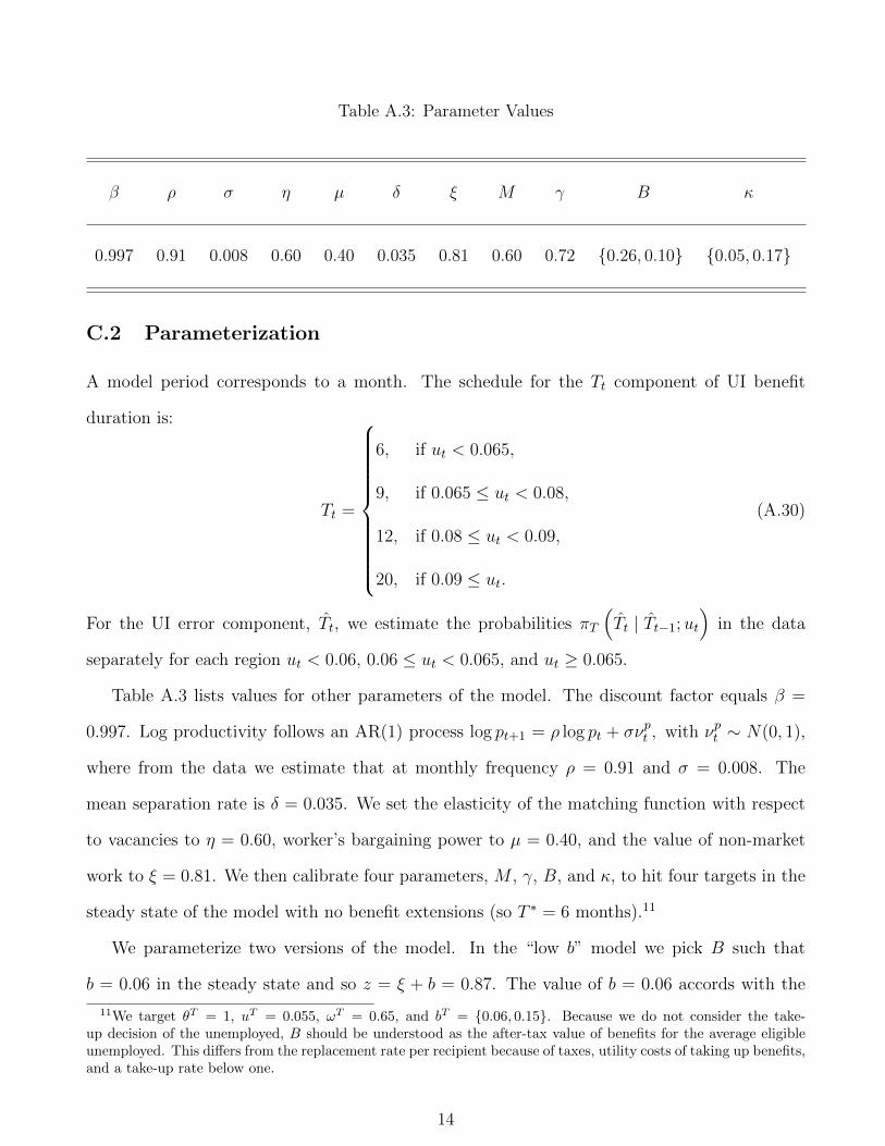
Table A.3: Parameter Values

β ρ σ η µ δ ξ M γ B κ

0.997 0.91 0.008 0.60 0.40 0.035 0.81 0.60 0.72 {0.26, 0.10} {0.05, 0.17}

C.2 Parameterization

A model period corresponds to a month. The schedule for the Tt component of UI benefit

duration is:

Tt =

6, if ut < 0.065,

9, if 0.065 ≤ ut < 0.08,

12, if 0.08 ≤ ut < 0.09,

20, if 0.09 ≤ ut.

(A.30)

For the UI error component, Tt, we estimate the probabilities πT

(Tt | Tt−1;ut

)in the data

separately for each region ut < 0.06, 0.06 ≤ ut < 0.065, and ut ≥ 0.065.

Table A.3 lists values for other parameters of the model. The discount factor equals β =

0.997. Log productivity follows an AR(1) process log pt+1 = ρ log pt + σνpt , with νpt ∼ N(0, 1),

where from the data we estimate that at monthly frequency ρ = 0.91 and σ = 0.008. The

mean separation rate is δ = 0.035. We set the elasticity of the matching function with respect

to vacancies to η = 0.60, worker’s bargaining power to µ = 0.40, and the value of non-market

work to ξ = 0.81. We then calibrate four parameters, M , γ, B, and κ, to hit four targets in the

steady state of the model with no benefit extensions (so T ∗ = 6 months).11

We parameterize two versions of the model. In the “low b” model we pick B such that

b = 0.06 in the steady state and so z = ξ + b = 0.87. The value of b = 0.06 accords with the

11We target θT = 1, uT = 0.055, ωT = 0.65, and bT = {0.06, 0.15}. Because we do not consider the take-up decision of the unemployed, B should be understood as the after-tax value of benefits for the average eligibleunemployed. This differs from the replacement rate per recipient because of taxes, utility costs of taking up benefits,and a take-up rate below one.

14

finding in Chodorow-Reich and Karabarbounis (2016) that benefits comprise a small fraction

of the average opportunity cost.12 In the “high b” model we pick B such that b = 0.15 and

z = ξ+ b = 0.96. The value of z = 0.96 was found by Hagedorn and Manovskii (2008) to match

the rigidity of wages with respect to productivity.

C.3 Computation

We solve the model globally by iterating on the equilibrium conditions. We begin by guessing

functions θ0(ut, ωt, pt, δt, Tt) and b0(ut, ωt, pt, δt, Tt) defined over grids of state variables. Given

these guesses, we obtain f(.), T (.), u′(.) and ω′(), where primes denote next period values, and

use equation (A.27) to obtain the wage function w(.). Next, we iterate on equation (A.25) to

solve for firm value J(.). Finally, we use the free-entry condition (A.26) and the definition of the

opportunity cost in equation (A.24) to obtain the implied θ1(.) and b1(.) functions. We update

the guesses and repeat until convergence. To evaluate value functions at points u′ and ω′ we

use linear interpolation. When solving for the equilibrium policy functions, we impose that the

probabilities f(.) and q(.) lie between zero and one. These restrictions also guarantee that v

and θ are always positive.

C.4 Additional Results

In Figures A.2, A.3, and A.4, we present the impulses of the fraction of unemployed receiving UI,

the log opportunity cost, and log vacancies to a one-month increase in the UI error innovation.

In Figures A.5 and A.6 we depict the path of productivity and separations shocks underlying

the experiment depicted in Figure 8 in the main text. In each figure, the left panel corresponds

to the high b model and the right panel corresponds to the low b model.

12Our calibration is conservative in the sense that reducing the level of ξ would produce even smaller effects of UIpolicy on aggregate outcomes. Chodorow-Reich and Karabarbounis (2016) show that, with standard preferences, zis between 0.47 and 0.75. Hornstein, Krusell, and Violante (2011) argue that z has to be even smaller in order formodels to generate large frictional wage dispersion. Hall and Mueller (2015) also arrive at a small value of z giventhe large observed dispersion in the value of a job. Costain and Reiter (2008) first pointed out that models with ahigh level of z generate stronger effects of policies on labor market outcomes than the effects found in cross-countrycomparisons.

15

0.1

.2.3

.4

Ch

an

ge

in F

ract

ion

Re

ceiv

ing

UI (P

P)

0 2 4 6 8

(a) High b Model

0.1

.2.3

.4

Ch

an

ge

in F

ract

ion

Re

ceiv

ing

UI (P

P)

0 2 4 6 8

(b) Low b Model

Figure A.2: Impulse Response of Fraction Receiving UI in the Model

Notes: The figure plots the coefficients on εt from the regression ωt+h = β(h)εt +∑11j=0 γj(h)ut−j + νt+h using

data generated from model simulations.

0.0

03

.00

6.0

09

.01

2

Ch

an

ge

in L

og

Op

po

rtu

nity

Co

st

0 2 4 6 8

(a) High b Model

0.0

03

.00

6.0

09

.01

2

Ch

an

ge

in L

og

Op

po

rtu

nity

Co

st

0 2 4 6 8

(b) Low b Model

Figure A.3: Impulse Response of Log Opportunity Cost in the Model

Notes: The figure plots the coefficients on εt from the regression log bt+h = β(h)εt +∑11j=0 γj(h)ut−j + νt+h using

data generated from model simulations.

16

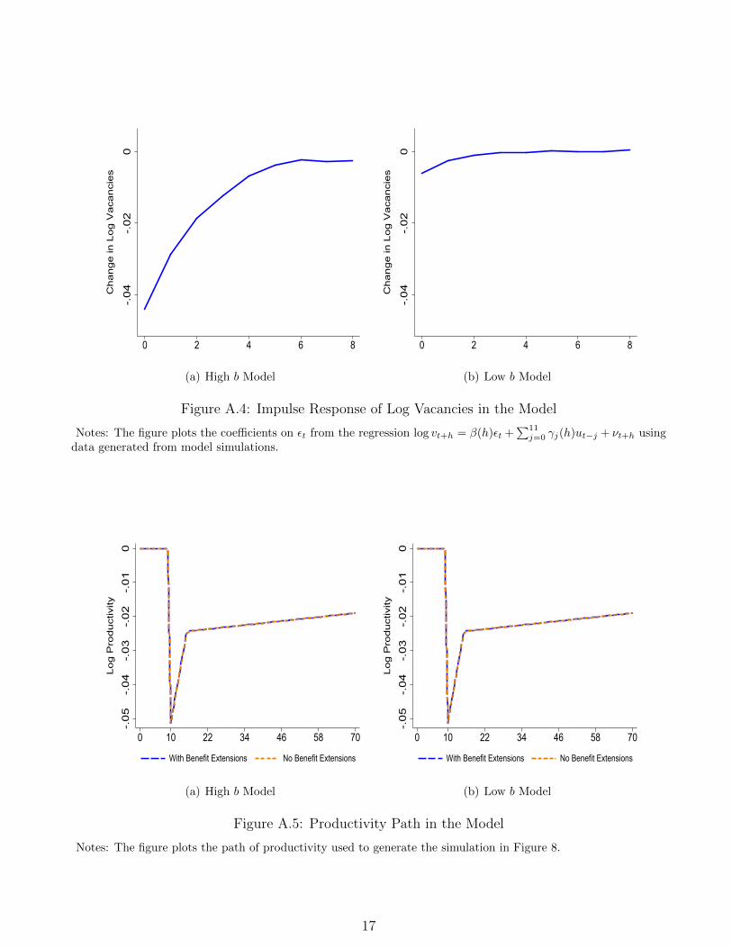
-.0

4-.

02

0

Ch

an

ge

in L

og

Va

can

cie

s

0 2 4 6 8

(a) High b Model

-.0

4-.

02

0

Ch

an

ge

in L

og

Va

can

cie

s

0 2 4 6 8

(b) Low b Model

Figure A.4: Impulse Response of Log Vacancies in the Model

Notes: The figure plots the coefficients on εt from the regression log vt+h = β(h)εt +∑11j=0 γj(h)ut−j + νt+h using

data generated from model simulations.

-.0

5-.

04

-.0

3-.

02

-.0

10

Lo

g P

rod

uct

ivity

0 10 22 34 46 58 70

With Benefit Extensions No Benefit Extensions

(a) High b Model

-.0

5-.

04

-.0

3-.

02

-.0

10

Lo

g P

rod

uct

ivity

0 10 22 34 46 58 70

With Benefit Extensions No Benefit Extensions

(b) Low b Model

Figure A.5: Productivity Path in the Model

Notes: The figure plots the path of productivity used to generate the simulation in Figure 8.

17

.03

.04

.05

.06

Se

pa

ratio

n R

ate

0 10 22 34 46 58 70

With Benefit Extensions No Benefit Extensions

(a) High b Model

.03

.04

.05

.06

Se

pa

ratio

n R

ate

0 10 22 34 46 58 70

With Benefit Extensions No Benefit Extensions

(b) Low b Model

Figure A.6: Separations in the Model

Notes: The figure plots the path of the separation rate used to generate the simulation in Figure 8.

18