The Link-Prediction Problem for Social Networkspersonal.stevens.edu/~jbao/BIA658A/Session10/liben-nowell.pdfThe Link-Prediction Problem for Social Networks ... 10.1002/asi.20591

Given a snapshot of a social network, can we infer whichnew interactions among its members are likely to occurin the near future? We formalize this question as the link-prediction problem, and we develop approaches to linkprediction based on measures for analyzing the “prox-imity” of nodes in a network. Experiments on large coau-thorship networks suggest that information about futureinteractions can be extracted from network topologyalone, and that fairly subtle measures for detecting nodeproximity can outperform more direct measures.

Introduction

As part of the recent surge of research on large, complexnetworks and their properties, a considerable amount of atten-tion has been devoted to the computational analysis of socialnetworks—structures whose nodes represent people or otherentities embedded in a social context, and whose edges repre-sent interaction, collaboration, or influence between entities.Natural examples of social networks include the set of all sci-entists in a particular discipline, with edges joining pairs whohave coauthored articles; the set of all employees in a largecompany, with edges joining pairs working on a common pro-ject; or a collection of business leaders, with edges joining pairswho have served together on a corporate board of directors. Theincreased availability of large, detailed datasets encoding suchnetworks has stimulated extensive study of their basic proper-ties, and the identification of recurring structural features (e.g.,see the work of Adamic & Adar, 2003; Grossman, 2002; New-man, 2002; Watts, 1999; Watts & Strogatz, 1998; for a thoroughrecent survey, see Newman, 2003).

Social networks are highly dynamic objects; they grow andchange quickly over time through the addition of new edges,signifying the appearance of new interactions in the underly-ing social structure. Identifying the mechanisms by whichthey evolve is a fundamental question that is still not wellunderstood, and it forms the motivation for our work here. We

define and study a basic computational problem underlyingsocial-network evolution, the link-prediction problem: Givena snapshot of a social network at time t, we seek to accuratelypredict the edges that will be added to the network during theinterval from time t to a given future time t�.

In effect, the link-prediction problem asks: To what extentcan the evolution of a social network be modeled using fea-tures intrinsic to the network itself ? Consider a coauthorshipnetwork among scientists, for example. There are many rea-sons exogenous to the network why two scientists who havenever written an article together will do so in the next fewyears: For example, they may happen to become geographi-cally close when one of them changes institutions. Such col-laborations can be hard to predict. But one also senses that alarge number of new collaborations are hinted at by thetopology of the network: Two scientists who are “close” inthe network will have colleagues in common and will travelin similar circles; this social proximity suggests that theythemselves are more likely to collaborate in the near future.Our goal is to make this intuitive notion precise and tounderstand which measures of “proximity” in a network leadto the most accurate link predictions. We find that a numberof proximity measures lead to predictions that outperformchance by factors of 40 to 50, indicating that the networktopology does indeed contain latent information from whichto infer future interactions. Moreover, certain fairly subtlemeasures—involving infinite sums over paths in thenetwork—often outperform more direct measures such asshortest-path distances and numbers of shared neighbors.

We believe that a primary contribution of the present articleis in the area of network-evolution models. While there hasbeen a proliferation of such models in recent years—e.g., see thework of Barabasi et al., 2002; Davidsen, Ebel, and Bornholdt,2002; Jin, Girvan, and Newman, 2001; for recent work on col-laboration networks, or the survey of Newman, 2003—thesemodels have generally been evaluated only by asking whetherthey reproduce certain global structural features observed inreal networks. As a result, it has been difficult to evaluate andcompare different approaches on a principled footing. Linkprediction, on the other hand, offers a very natural basis for

JOURNAL OF THE AMERICAN SOCIETY FOR INFORMATION SCIENCE AND TECHNOLOGY, 58(7):1019–1031, 2007

The Link-Prediction Problem for Social Networks

David Liben-NowellDepartment of Computer Science, Carleton College, Northfield, MN 55057. E-mail: [email protected]

Jon KleinbergDepartment of Computer Science, Cornell University, Ithaca, NY 14853. E-mail: [email protected]

Received June 16, 2005; revised July 5, 2006; accepted August 25, 2006

© 2007 Wiley Periodicals, Inc. • Published online 26 March 2007 in WileyInterScience (www.interscience.wiley.com). DOI: 10.1002/asi.20591

1020 JOURNAL OF THE AMERICAN SOCIETY FOR INFORMATION SCIENCE AND TECHNOLOGY—May 2007DOI: 10.1002/asi

such evaluations: A network model is useful to the extent that itcan support meaningful inferences from observed networkdata. One sees a related approach in recent work of Newman(2001a), who considers the correlation between certain net-work-growth models and data on the appearance of edges ofcoauthorship networks.

In addition to its role as a basic question in social-networkevolution, the link-prediction problem could be relevant to anumber of interesting current applications of social networks.Increasingly, for example, researchers in artificial intelligenceand data mining have argued that a large organization (e.g., acompany) can benefit from the interactions within the informalsocial network among its members; these ties serve to supple-ment the official hierarchy imposed by the organization itself(Kautz, Selman, & Shah, 1997; Raghavan, 2002). Effectivemethods for link prediction could be used to analyze such asocial network to suggest promising interactions or collabora-tions that have not yet been identified within the organization.In a different vein, research in security has recently begun toemphasize the role of social-network analysis, largely moti-vated by the problem of monitoring terrorist networks; linkprediction in this context allows one to conjecture that particu-lar individuals are working together even though their interac-tion has not been directly observed (Krebs, 2002).

The link-prediction problem also is related to the problemof inferring missing links from an observed network: In a num-ber of domains, one constructs a network of interactions basedon observable data and then tries to infer additional links that,while not directly visible, are likely to exist (Goldberg & Roth,2003; Popescul & Ungar, 2003; Taskar, Wong, Abbeel, &Koller, 2003). This line of work differs from our problem for-mulation in that it works with a static snapshot of a networkrather than considering network evolution; it also tends to takeinto account specific attributes of the nodes in the networkrather than evaluating the power of prediction methods that arebased purely on the graph structure.

We turn to a description of our experimental setup in thenext section. Our primary focus is on understanding the rel-ative effectiveness of network-proximity measures adaptedfrom techniques in graph theory, computer science, and thesocial sciences, and we review a large number of such tech-niques. Finally, we discuss the results of our experiments.

Data and Experimental Setup

Suppose that we have a social network in whicheach edge represents an interaction betweenu and v that took place at a particular time t(e). We record multipleinteractions between u and v as parallel edges, with potentiallydifferent timestamps. For two times t � , let G[t, ] denote thesubgraph of G consisting of all edges with a timestamp betweent and . Here, then, is a concrete formulation of the link-predictionproblem. We choose four times t0 � � t1 � and give analgorithm access to the network G[t0, ]; it must then output a listof edges not present in G[t0, ] that are predicted to appear in thenetwork G[t1, ]. We refer to [t0, ] as the training interval and[t1, ] as the test interval.t�1

t�0t�1

t�0

t�0

t�1t�0

t�

t�t�

e � 8u, v 9 � EG � 8V, E 9

Of course, social networks grow through the addition ofnodes as well as edges, and it is not sensible to seek predic-tions for edges whose endpoints are not present in the traininginterval. Thus, in evaluating link-prediction methods, we willgenerally use two parameters, training and test, and definethe set Core to consist of all nodes that are incident to at least

training edges in G[t0, ] and at least test edges in G[t1, ]. Wewill then evaluate how accurately the new edges betweenelements of Core can be predicted.

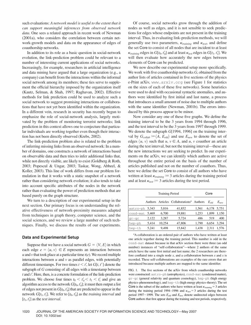
We now describe our experimental setup more specifically.We work with five coauthorship networks G, obtained from theauthor lists of articles contained in five sections of the physicse-Print arXiv, www.arxiv.org (see Figure 1 for statisticson the sizes of each of these five networks). Some heuristicswere used to deal with occasional syntactic anomalies, and au-thors were identified by first initial and last name, a processthat introduces a small amount of noise due to multiple authorswith the same identifier (Newman, 2001b). The errors intro-duced by this process appear to be minor.

Now consider any one of these five graphs. We define thetraining interval to be the 3 years from 1994 through 1996,and the test interval to be the 3 years from 1997 through 1999.We denote the subgraph G[1994, 1996] on the training inter-val by Gcollab A, Eold and use Enew to denote the set ofedges u, v such that u, v A, and u, v coauthor an articleduring the test interval, but not the training interval—these arethe new interactions we are seeking to predict. In our experi-ments on the arXiv, we can identify which authors are activethroughout the entire period on the basis of the number ofarticles published and not on the number of coauthors. Thus,here we define the set Core to consist of all authors who havewritten at least training 3 articles during the training periodand at least test 3 articles during the test period.Jk

Jk

�98 98J

t�1kt�0k

kk

Training Period Core

Authors Articles Collaborationsa Authors Eold Enew

astro-ph 5,343 5,816 41,852 1,561 6,178 5,751

cond-mat 5,469 6,700 19,881 1,253 1,899 1,150

gr-qc 2,122 3,287 5,724 486 519 400

hep-ph 5,414 10,254 47,806 1,790 6,654 3,294

hep-th 5,241 9,498 15,842 1,438 2,311 1,576

aA collaboration is an ordered pair of authors who have written at leastone article together during the training period. This number is odd in thecond-mat dataset because in that arXiv section there were three (an oddnumber) instances of “self-collaboration”—where 2 authors of the samearticle have the same first initial and last name; the 2 researchers are there-fore conflated into a single node x, and a collaboration between x and x isrecorded. These self-collaborations are examples of the rare errors that areintroduced because multiple authors are mapped to the same identifier.

FIG. 1. The five sections of the arXiv from which coauthorship networkswere constructed: astro-ph (astrophysics), cond-mat (condensed matter),gr-qc (general relativity and quantum cosmology), hep-ph (high energyphysics–phenomenology), and hep-th (high energy physics–theory). The setCore is the subset of the authors who have written at least training � 3 articlesduring the training period 1994–1996 and test � 3 articles during the testperiod 1997�1999. The sets Eold and Enew denote undirected edges betweenCore authors that first appear during the training and test periods, respectively.

k

k

JOURNAL OF THE AMERICAN SOCIETY FOR INFORMATION SCIENCE AND TECHNOLOGY—May 2007 1021DOI: 10.1002/asi

Evaluating a Link Predictor

Each link predictor p that we consider outputs a ranked listLp of pairs in A � A � Eold; these are predicted new collabora-tions, in decreasing order of confidence. For our evaluation, wefocus on the set Core, so we define (Core �Core) and . Our performance measure for Predictor pis then determined as follows: From the ranked list Lp, we takethe first n pairs that are in Core � Core, and determine the sizeof the intersection of this set of pairs with the set .

Methods for Link Prediction

In this section, we survey an array of methods for link pre-diction. All the methods assign a connection weight score(x, y)to pairs of nodes x, y , based on the input graph Gcollab, andthen produce a ranked list in decreasing order of score(x, y).Thus, they can be viewed as computing a measure of proxim-ity or “similarity” between nodes x and y, relative to thenetwork topology. In general, the methods are adapted fromtechniques used in graph theory and in social-network analy-sis; in a number of cases, these techniques were not designedto measure node-to-node similarity and hence need to bemodified for this purpose. Figure 2 summarizes most of thesemeasures; we discuss them in more detail later. Note that

98

Enew�

n J |Enew� |

xEnew� J Enew

some of these measures are designed only for connectedgraphs; because each graph Gcollab that we consider has a giantcomponent—a single component containing most of thenodes—it is natural to restrict the predictions for these mea-sures to this component.

Perhaps the most basic approach is to rank pairs x, y bythe length of their shortest path in Gcollab. Such a measurefollows the notion that collaboration networks are “smallworlds,” in which individuals are related through shortchains (Newman, 2001b) (In keeping with the notion thatwe rank pairs in decreasing order of score(x, y), we definescore(x, y) here to be the negative of the shortest pathlength.) Pairs with shortest-path distance equal to oneare joined by an edge in Gcollab, and hence they belong tothe training edge set Eold. For all of our graphs Gcollab, thereare well more than n pairs at shortest-path distance two, soour shortest-path predictor simply selects a random subset ofthese distance-two pairs.

Methods Based on Node Neighborhoods

For a node x, let �(x) denote the set of neighbors of x inGcollab. A number of approaches are based on the idea that twonodes x and y are more likely to form a link in the future iftheir sets of neighbors �(x) and �(y) have large overlap; this

98

FIG. 2. Values for score(x, y) under various predictors; each predicts pairs x, y in descending order ofscore(x, y). The set �(x) consists of the neighbors of the node x in Gcollab.

98

graph distance (negated) length of shortest path between x and y

common neighbors

Jaccard’s coefficient

Adamic/Adar

preferential attachment

Katzb

where paths {paths of length exactly from x to y}

weighted: paths number of collaborations between x, y.

unweighted: paths iff x and y collaborate.

hitting time �Hx,y

stationary-normed �Hx,y y

commute time �(Hx,y � Hy,x)stationary-normed �Hx,y y � Hy,x x)

where Hx,y expected time for random walk from x to reach y

y stationary-distribution weight of y (proportion of time the random walk is at node y)

rooted PageRank stationary distribution weight of y under the following random walk: with probability , jump to x. with probability 1 � , go to a random neighbor of current node.

SimRank•1 if x�y

g #©a��(x)©b��(y) score(a, b)

��(x)� # ��(y)�otherwiseg

a

aa

JpJ

p#p#

p#

�1�x,y J 1

�1�x,y J

Ox,y�O�

J

©��1b

/ 0paths�O�x,y 0

0 ≠ (x) 0 0 ≠(y) 0©z�≠(x)t≠(y)

1log 0≠(z) 0

0 ≠(x) � ≠(y) 00 ≠ (x) ´ ≠(y) 0

0 ≠ (x) � ≠(y) 0


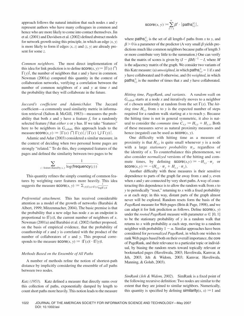
approach follows the natural intuition that such nodes x and yrepresent authors who have many colleagues in common andhence who are more likely to come into contact themselves. Jinet al. (2001) and Davidsen et al. (2002) defined abstract modelsfor network growth using this principle, in which an edge x, yis more likely to form if edges x, z and z, y are already pre-sent for some z.

Common neighbors. The most direct implementation ofthis idea for link prediction is to define score(x, y) �(x) �(y), the number of neighbors that x and y have in common.Newman (2001a) computed this quantity in the context of collaboration networks, verifying a correlation between thenumber of common neighbors of x and y at time t andthe probability that they will collaborate in the future.

Jaccard’s coefficient and Adamic/Adar. The Jaccardcoefficient—a commonly used similarity metric in informa-tion retrieval (Salton & McGill, 1983)—measures the prob-ability that both x and y have a feature f, for a randomlyselected feature f that either x or y has. If we take “features”here to be neighbors in Gcollab, this approach leads to themeasure

Adamic and Adar (2003) considered a similar measure, inthe context of deciding when two personal home pages arestrongly “related.” To do this, they computed features of thepages and defined the similarity between two pages to be

This quantity refines the simply counting of common fea-tures by weighting rarer features more heavily. This ideasuggests the measure score(x, y)

Preferential attachment. This has received considerableattention as a model of the growth of networks (Barabási &Albert, 1999; Mitzenmacher, 2004). The basic premise is thatthe probability that a new edge has node x as an endpoint isproportional to |�(x)|, the current number of neighbors of x.Newman (2001a) and Barabási et al. (2002) further proposed,on the basis of empirical evidence, that the probability ofcoauthorship of x and y is correlated with the product of thenumber of collaborators of x and y. This proposal corre-sponds to the measure score(x, y) |�(x)| |�(y)|.

Methods Based on the Ensemble of All Paths

A number of methods refine the notion of shortest-pathdistance by implicitly considering the ensemble of all pathsbetween two nodes.

Katz (1953). Katz defined a measure that directly sums overthis collection of paths, exponentially damped by length tocount short paths more heavily. This notion leads to the measure

J

©z��(x)t�(y)1

log|�(z)|.J

az : feature shared by x, y

1

log(frequency(z) ).

score(x,y) J ƒ �(x) x �(y) ƒ � ƒ �(x) h �(y) ƒ .

xJ

989898 where is the set of all length- paths from x to y, and

� 0 is a parameter of the predictor (A very small yields pre-dictions much like common neighbors because paths of length 3or more contribute very little to the summation.) One can verifythat the matrix of scores is given by (I � M)�1 � I, where Mis the adjacency matrix of the graph. We consider two variants ofthis Katz measure: (a) unweighted, in which � 1 if x andy have collaborated and 0 otherwise, and (b) weighted, in which

is the number of times that x and y have collaborated.

Hitting time, PageRank, and variants. A random walk onGcollab starts at a node x and iteratively moves to a neighborof x chosen uniformly at random from the set �(x). The hit-ting time Hx,y from x to y is the expected number of stepsrequired for a random walk starting at x to reach y. Becausethe hitting time is not in general symmetric, it also is nat-ural to consider the commute time Cx,y Hx,y � Hy, x. Bothof these measures serve as natural proximity measures andhence (negated) can be used as score(x, y).

One difficulty with hitting time as a measure ofproximity is that Hx,y is quite small whenever y is a nodewith a large stationary probability y, regardless ofthe identity of x. To counterbalance this phenomenon, wealso consider normalized versions of the hitting and com-mute times, by defining or

Another difficulty with these measures is their sensitivedependence to parts of the graph far away from x and y, evenwhen x and y are connected by very short paths. A way of coun-teracting this dependence is to allow the random walk from x toy to periodically “reset,” returning to x with a fixed probability

at each step; in this way, distant parts of the graph almostnever will be explored. Random resets form the basis of thePageRank measure for Web pages (Brin & Page, 1998), and wecan adapt it for link prediction as follows. Define score(x, y)under the rooted PageRank measure with parameter [0, 1]to be the stationary probability of y in a random walk thatreturns to x with probability each step, moving to a randomneighbor with probability 1 � . Similar approaches have beenconsidered for personalized PageRank, in which one wishes torank Web pages based both on their overall importance, the coreof PageRank, and their relevance to a particular topic or individ-ual, by biasing the random resets toward topically relevant orbookmarked pages (Haveliwala, 2003; Haveliwala, Kamvar, &Jeh, 2003; Jeh & Widom, 2003; Kamvar, Haveliwala,Manning, & Golub, 2003).

SimRank (Jeh & Widom, 2002). SimRank is a fixed point ofthe following recursive definition: Two nodes are similar to theextent that they are joined to similar neighbors. Numerically,this quantity is specified by defining similarity(x, x) 1 andJ

a

a

�a

a

score(x,y) J �(Hx,y# py � Hy, x

# px).score(x,y) J �Hx,y

# py

p

J

pathsx,y�1�

pathsx,y�1�

b

bb

/pathsx,y�/�

score(x, y) Ja�

/�1

b/ # ƒ pathsx,y8/9 ƒ ,


for a parameter � [0, 1]. We then define score(x, y)similarity(x, y). SimRank also can be interpreted in terms ofa random walk on the collaboration graph: It is the expectedvalue of , where is a random variable giving the time atwhich random walks started from x and y first meet.

Higher Level Approaches

We now discuss three “meta-approaches” that can be usedin conjunction with any of the methods discussed earlier.

Low-rank approximation. Because the adjacency matrixM can be used to represent the graph Gcollab, all of our link-prediction methods have an equivalent formulation in termsof this matrix M. In some cases, this correspondence wasnoted explicitly earlier (e.g., in the case of the Katz similar-ity score), but in many other cases the matrix formulationalso is quite natural. For example, the common-neighborsmethod consists simply of mapping each node x to its rowr(x) in M, and then defining score(x, y) to be the inner prod-uct of the rows r(x) and r(y).

A common general technique when analyzing thestructure of a large matrix M is to choose a relatively smallnumber k and compute the rank-k matrix Mk that bestapproximates M with respect to any of a number of standardmatrix norms. This computation can be done efficiently usingthe singular-value decomposition, and it forms the core ofmethods such as latent semantic analysis in informationretrieval (Deerwester, Dumais, Furnas, Landauer, & Harshman,1990). Intuitively, working with Mk rather than M can beviewed as a type of “noise-reduction” technique that gener-ates most of the structure in the matrix, but with a greatlysimplified representation.

In our experiments, we investigate three applications of low-rank approximation: (a) ranking by the Katz measure, in whichwe use Mk rather than M in the underlying formula; (b) rankingby common neighbors, in which we score by inner products ofrows in Mk rather than M; and—most simply of all—(c) defin-ing score(x, y) to be the x, y entry in the matrix Mk.

Unseen bigrams. Link prediction is akin to the problem ofestimating frequencies for unseen bigrams in languagemodeling—pairs of words that co-occur in a test corpus, butnot in the corresponding training corpus (e.g., see the workof Essen & Steinbiss, 1992). Following ideas proposed inthat literature (e.g., Lee, 1999), we can augment our esti-mates for score(x, y) using values of score(z, y) for nodes zthat are “similar” to x. Specifically, we adapt this approach tothe link-prediction problem as follows. Suppose we havevalues score(x, y) computed under one of the measuresabove. Let denote the nodes most related to x underscore(x,), for a parameter ZZ�. We then define enhancedd �

dSx�d�

98

/g/

J�

similarity(x, y) :� g # ©a��(x) ©b��(y)similarity(a, b)

ƒ �(x) ƒ # ƒ �(y) ƒscores in terms of the nodes in this set:

Clustering. One might seek to improve on the quality of apredictor by deleting the more “tenuous” edges in Gcollab

through a clustering procedure, and then running the predictoron the resulting “cleaned-up” subgraph. Consider a measurecomputing values for score(x, y). We compute score(u, v) for alledges in Eold, and delete the (1� ) fraction of these edges forwhich the score is lowest, for a parameter . We nowrecompute score(x, y) for all pairs x, y on this subgraph; in thisway, we determine node proximities using only edges for whichthe proximity measure itself has the most confidence.

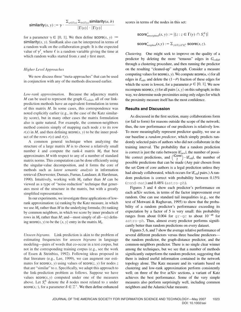
Results and Discussion

As discussed in the first section, many collaborations form(or fail to form) for reasons outside the scope of the network;thus, the raw performance of our predictors is relatively low.To more meaningfully represent predictor quality, we use asour baseline a random predictor, which simply predicts ran-domly selected pairs of authors who did not collaborate in thetraining interval. The probability that a random predictionis correct is just the ratio between |Enew|, the number of possi-ble correct predictions, and |Eold|, the number ofpossible predictions that can be made (Any pair chosen fromthe set Core of core authors is a legal prediction unless theyhad already collaborated, which occurs for |Eold| pairs.) A ran-dom prediction is correct with probability between 0.15%(cond-mat) and 0.48% (astro-ph).

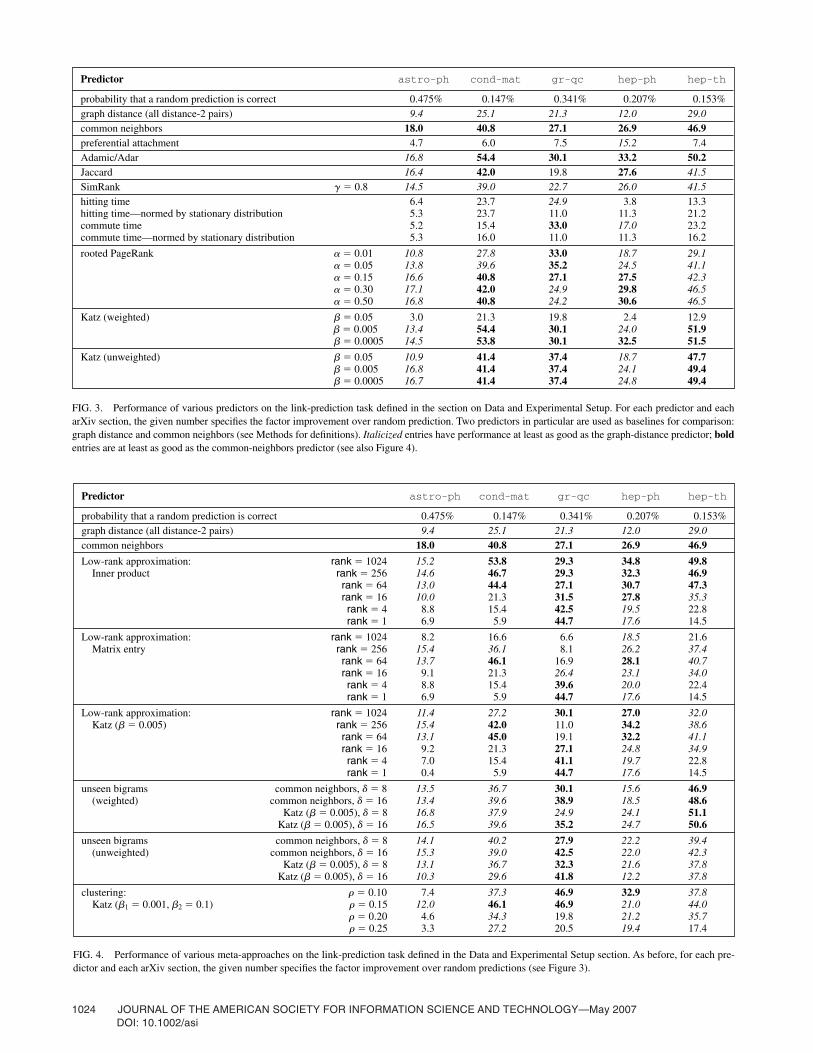
Figures 3 and 4 show each predictor’s performance oneach arXiv section, in terms of the factor improvement overrandom. One can use standard tail inequalities (e.g., see thetext of Motwani & Raghavan, 1995) to show that the proba-bility of a random predictor’s performance exceeding itsexpectation by a factor of 5 is very small: this probabilityranges from about 0.004 for gr-qc to about 10�48 forastro-ph. Thus, almost every predictor performs signifi-cantly better than random predictions on every dataset.

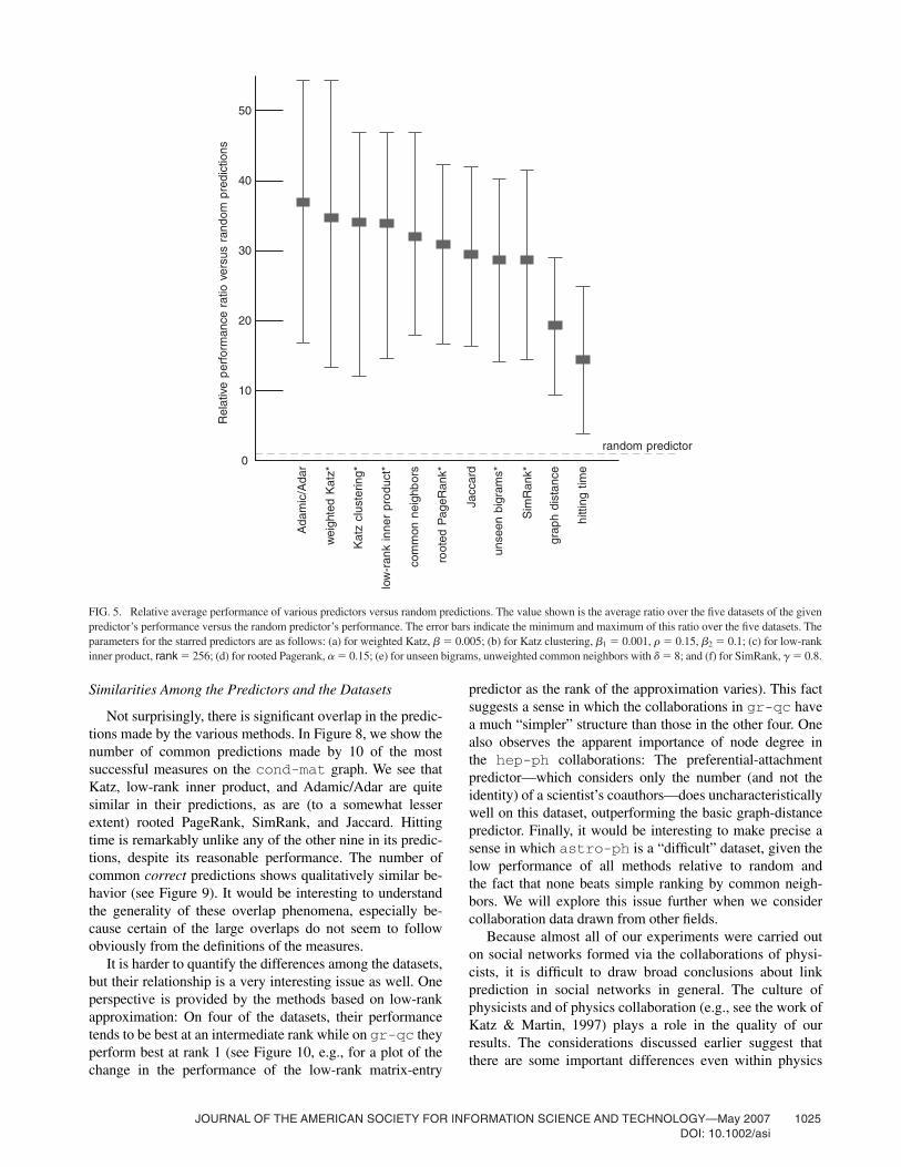
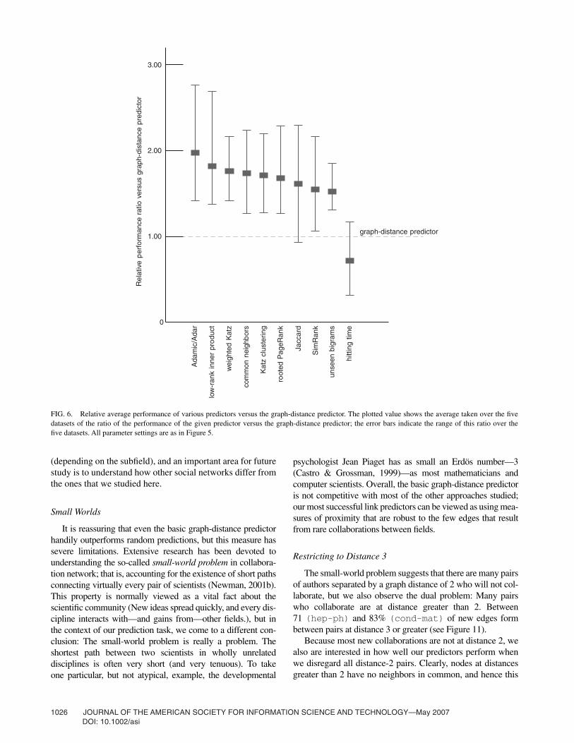
Figures 5, 6, and 7 show the average relative performance ofseveral different predictors versus three baseline predictors—the random predictor, the graph-distance predictor, and thecommon-neighbors predictor. There is no single clear winneramong the techniques, but we see that a number of methodssignificantly outperform the random predictor, suggesting thatthere is indeed useful information contained in the networktopology alone. The Katz measure and its variants based onclustering and low-rank approximation perform consistentlywell; on three of the five arXiv sections, a variant of Katzachieves the best performance. Some of the very simplemeasures also perform surprisingly well, including commonneighbors and the Adamic/Adar measure.

Q |Core|R2 �

98r� [0, 1]

r

scoreweighted� (x,y) :� ©z��(y)tSx

�d� score(x, z).

scoreunweighted� (x, y) :� ƒ{z : z � �(y) � Sx

�d�} ƒ


Predictor astro-ph cond-mat gr-qc hep-ph hep-th

probability that a random prediction is correct 0.475% 0.147% 0.341% 0.207% 0.153%graph distance (all distance-2 pairs) 9.4 25.1 21.3 12.0 29.0common neighbors 18.0 40.8 27.1 26.9 46.9preferential attachment 4.7 6.0 7.5 15.2 7.4Adamic/Adar 16.8 54.4 30.1 33.2 50.2Jaccard 16.4 42.0 19.8 27.6 41.5SimRank g� 0.8 14.5 39.0 22.7 26.0 41.5hitting time 6.4 23.7 24.9 3.8 13.3hitting time—normed by stationary distribution 5.3 23.7 11.0 11.3 21.2commute time 5.2 15.4 33.0 17.0 23.2commute time—normed by stationary distribution 5.3 16.0 11.0 11.3 16.2

rooted PageRank a � 0.01 10.8 27.8 33.0 18.7 29.1a � 0.05 13.8 39.6 35.2 24.5 41.1a � 0.15 16.6 40.8 27.1 27.5 42.3a � 0.30 17.1 42.0 24.9 29.8 46.5a � 0.50 16.8 40.8 24.2 30.6 46.5

Katz (weighted) b� 0.05 3.0 21.3 19.8 2.4 12.9b� 0.005 13.4 54.4 30.1 24.0 51.9b� 0.0005 14.5 53.8 30.1 32.5 51.5

Katz (unweighted) b� 0.05 10.9 41.4 37.4 18.7 47.7b� 0.005 16.8 41.4 37.4 24.1 49.4b� 0.0005 16.7 41.4 37.4 24.8 49.4

FIG. 3. Performance of various predictors on the link-prediction task defined in the section on Data and Experimental Setup. For each predictor and eacharXiv section, the given number specifies the factor improvement over random prediction. Two predictors in particular are used as baselines for comparison:graph distance and common neighbors (see Methods for definitions). Italicized entries have performance at least as good as the graph-distance predictor; boldentries are at least as good as the common-neighbors predictor (see also Figure 4).


probability that a random prediction is correct 0.475% 0.147% 0.341% 0.207% 0.153%graph distance (all distance-2 pairs) 9.4 25.1 21.3 12.0 29.0common neighbors 18.0 40.8 27.1 26.9 46.9

Low-rank approximation: rank � 1024 15.2 53.8 29.3 34.8 49.8Inner product rank � 256 14.6 46.7 29.3 32.3 46.9

rank � 64 13.0 44.4 27.1 30.7 47.3rank � 16 10.0 21.3 31.5 27.8 35.3rank � 4 8.8 15.4 42.5 19.5 22.8rank � 1 6.9 5.9 44.7 17.6 14.5

Low-rank approximation: rank � 1024 8.2 16.6 6.6 18.5 21.6Matrix entry rank � 256 15.4 36.1 8.1 26.2 37.4


Low-rank approximation: rank � 1024 11.4 27.2 30.1 27.0 32.0Katz (b� 0.005) rank � 256 15.4 42.0 11.0 34.2 38.6


unseen bigrams common neighbors, d � 8 13.5 36.7 30.1 15.6 46.9(weighted) common neighbors, d � 16 13.4 39.6 38.9 18.5 48.6

Katz (b� 0.005), d � 8 16.8 37.9 24.9 24.1 51.1Katz (b� 0.005), d � 16 16.5 39.6 35.2 24.7 50.6

unseen bigrams common neighbors, d � 8 14.1 40.2 27.9 22.2 39.4(unweighted) common neighbors, d � 16 15.3 39.0 42.5 22.0 42.3

Katz (b� 0.005), d � 8 13.1 36.7 32.3 21.6 37.8Katz (b� 0.005), d � 16 10.3 29.6 41.8 12.2 37.8

clustering: r� 0.10 7.4 37.3 46.9 32.9 37.8Katz (b1 � 0.001, b2 � 0.1) r� 0.15 12.0 46.1 46.9 21.0 44.0

r� 0.20 4.6 34.3 19.8 21.2 35.7r� 0.25 3.3 27.2 20.5 19.4 17.4

FIG. 4. Performance of various meta-approaches on the link-prediction task defined in the Data and Experimental Setup section. As before, for each pre-dictor and each arXiv section, the given number specifies the factor improvement over random predictions (see Figure 3).


FIG. 5. Relative average performance of various predictors versus random predictions. The value shown is the average ratio over the five datasets of the givenpredictor’s performance versus the random predictor’s performance. The error bars indicate the minimum and maximum of this ratio over the five datasets. Theparameters for the starred predictors are as follows: (a) for weighted Katz, � 0.005; (b) for Katz clustering, 1 � 0.001, � 0.15, 2 � 0.1; (c) for low-rankinner product, rank � 256; (d) for rooted Pagerank, � 0.15; (e) for unseen bigrams, unweighted common neighbors with � 8; and (f) for SimRank, � 0.8.gda

brbb

0

10

20

30

40

50

Rel

ativ

ep

erfo

rman

cera

tiove

rsus

rand

ompr

edic

tions

random predictor

Ada

mic

/Ada

r

wei

ghte

dK

atz*

Kat

zcl

uste

ring*

low

-ran

kin

ner

pro

duct

*

com

mon

neig

hbor

s

root

edP

ageR

ank*

Jacc

ard

unse

enbi

gram

s*

Sim

Ran

k*

grap

hdi

stan

ce

hitti

ngtim

e

Similarities Among the Predictors and the Datasets

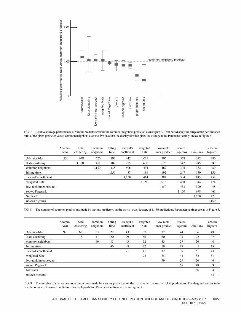
Not surprisingly, there is significant overlap in the predic-tions made by the various methods. In Figure 8, we show thenumber of common predictions made by 10 of the mostsuccessful measures on the cond-mat graph. We see thatKatz, low-rank inner product, and Adamic/Adar are quitesimilar in their predictions, as are (to a somewhat lesserextent) rooted PageRank, SimRank, and Jaccard. Hittingtime is remarkably unlike any of the other nine in its predic-tions, despite its reasonable performance. The number ofcommon correct predictions shows qualitatively similar be-havior (see Figure 9). It would be interesting to understandthe generality of these overlap phenomena, especially be-cause certain of the large overlaps do not seem to followobviously from the definitions of the measures.

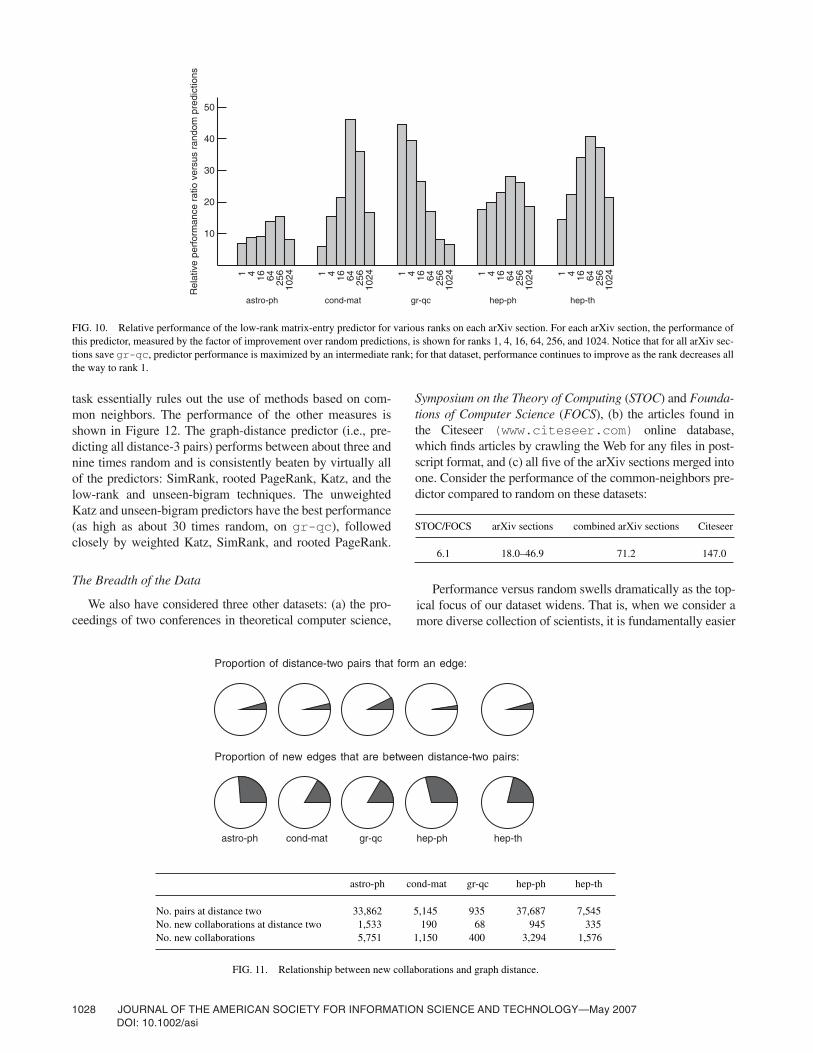
It is harder to quantify the differences among the datasets,but their relationship is a very interesting issue as well. Oneperspective is provided by the methods based on low-rankapproximation: On four of the datasets, their performancetends to be best at an intermediate rank while on gr-qc theyperform best at rank 1 (see Figure 10, e.g., for a plot of thechange in the performance of the low-rank matrix-entry

predictor as the rank of the approximation varies). This factsuggests a sense in which the collaborations in gr-qc havea much “simpler” structure than those in the other four. Onealso observes the apparent importance of node degree inthe hep-ph collaborations: The preferential-attachmentpredictor—which considers only the number (and not theidentity) of a scientist’s coauthors—does uncharacteristicallywell on this dataset, outperforming the basic graph-distancepredictor. Finally, it would be interesting to make precise asense in which astro-ph is a “difficult” dataset, given thelow performance of all methods relative to random andthe fact that none beats simple ranking by common neigh-bors. We will explore this issue further when we considercollaboration data drawn from other fields.

Because almost all of our experiments were carried outon social networks formed via the collaborations of physi-cists, it is difficult to draw broad conclusions about linkprediction in social networks in general. The culture ofphysicists and of physics collaboration (e.g., see the work ofKatz & Martin, 1997) plays a role in the quality of ourresults. The considerations discussed earlier suggest thatthere are some important differences even within physics


0

1.00

2.00

3.00

Rel

ativ

ep

erfo

rman

cera

tiove

rsus

grap

h-di

stan

cepr

edic

tor

graph-distance predictor

Ada

mic

/Ada

r

low

-ran

kin

ner

pro

duct

wei

ghte

dK

atz

com

mon

neig

hbor

s

Kat

zcl

uste

ring

root

edP

ageR

ank

Jacc

ard

Sim

Ran

k

unse

enbi

gram

s

hitti

ngtim

e

FIG. 6. Relative average performance of various predictors versus the graph-distance predictor. The plotted value shows the average taken over the fivedatasets of the ratio of the performance of the given predictor versus the graph-distance predictor; the error bars indicate the range of this ratio over thefive datasets. All parameter settings are as in Figure 5.

(depending on the subfield), and an important area for futurestudy is to understand how other social networks differ fromthe ones that we studied here.

Small Worlds

It is reassuring that even the basic graph-distance predictorhandily outperforms random predictions, but this measure hassevere limitations. Extensive research has been devoted tounderstanding the so-called small-world problem in collabora-tion network; that is, accounting for the existence of short pathsconnecting virtually every pair of scientists (Newman, 2001b).This property is normally viewed as a vital fact about thescientific community (New ideas spread quickly, and every dis-cipline interacts with—and gains from—other fields.), but inthe context of our prediction task, we come to a different con-clusion: The small-world problem is really a problem. Theshortest path between two scientists in wholly unrelateddisciplines is often very short (and very tenuous). To takeone particular, but not atypical, example, the developmental

psychologist Jean Piaget has as small an Erdös number—3(Castro & Grossman, 1999)—as most mathematicians andcomputer scientists. Overall, the basic graph-distance predictoris not competitive with most of the other approaches studied;our most successful link predictors can be viewed as using mea-sures of proximity that are robust to the few edges that resultfrom rare collaborations between fields.

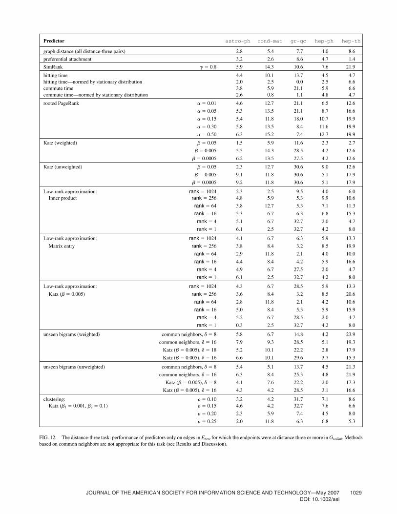
Restricting to Distance 3

The small-world problem suggests that there are many pairsof authors separated by a graph distance of 2 who will not col-laborate, but we also observe the dual problem: Many pairswho collaborate are at distance greater than 2. Between71 (hep-ph) and 83% (cond-mat) of new edges formbetween pairs at distance 3 or greater (see Figure 11).

Because most new collaborations are not at distance 2, wealso are interested in how well our predictors perform whenwe disregard all distance-2 pairs. Clearly, nodes at distancesgreater than 2 have no neighbors in common, and hence this


Adamic/ Katz common hitting Jaccard’s weighted low-rank rooted unseen Adar clustering neighbors time coefficient Katz inner product Pagerank SimRank bigrams

Adamic/Adar 1,150 638 520 193 442 1,011 905 528 372 486

Katz clustering 1,150 411 182 285 630 623 347 245 389

common neighbors 1,150 135 506 494 467 305 332 489

hitting time 1,150 87 191 192 247 130 156

Jaccard’s coefficient 1,150 414 382 504 845 458

weighted Katz 1,150 1,013 488 344 474

low-rank inner product 1,150 453 320 448

rooted Pagerank 1,150 678 461

SimRank 1,150 423

unseen bigrams 1,150

FIG. 8. The number of common predictions made by various predictors on the cond-mat dataset, of 1,150 predictions. Parameter settings are as in Figure 5.

Adamic/ Katz common hitting Jaccard’s weighted low-rank rooted unseen Adar clustering neighbors time coefficient Katz inner product Pagerank SimRank bigrams

Adamic/Adar 92 65 53 22 43 87 72 44 36 49

Katz clustering 78 41 20 29 66 60 31 22 37

common neighbors 69 13 43 52 43 27 26 40

hitting time 40 8 22 19 17 9 15

Jaccard’s coefficient 71 41 32 39 51 43

weighted Katz 92 75 44 32 51

low-rank inner product 79 39 26 46

rooted Pagerank 69 48 39

SimRank 66 34

unseen bigrams 68

FIG. 9. The number of correct common predictions made by various predictors on the cond-mat dataset, of 1,150 predictions. The diagonal entries indi-cate the number of correct predictions for each predictor. Parameter settings are as in Figure 5.

0

1.00

2.00

Rel

ativ

ep

erfo

rman

cera

tiove

rsus

com

mon

-nei

ghb

ors

pred

icto

rcommon-neighbors predictor

Ada

mic

/Ada

r

Kat

zcl

uste

ring

low

-ran

kin

ner

pro

duct

wei

ghte

dK

atz

root

edP

ageR

ank

Jacc

ard

unse

enbi

gram

s

Sim

Ran

k

grap

hdi

stan

ce

hitti

ngtim

e

FIG. 7. Relative average performance of various predictors versus the common-neighbors predictor, as in Figure 6. Error bars display the range of the performanceratio of the given predictor versus common neighbors over the five datasets; the displayed value gives the average ratio. Parameter settings are as in Figure 5.


task essentially rules out the use of methods based on com-mon neighbors. The performance of the other measures isshown in Figure 12. The graph-distance predictor (i.e., pre-dicting all distance-3 pairs) performs between about three andnine times random and is consistently beaten by virtually allof the predictors: SimRank, rooted PageRank, Katz, and thelow-rank and unseen-bigram techniques. The unweightedKatz and unseen-bigram predictors have the best performance(as high as about 30 times random, on gr-qc), followedclosely by weighted Katz, SimRank, and rooted PageRank.

The Breadth of the Data

We also have considered three other datasets: (a) the pro-ceedings of two conferences in theoretical computer science,

Symposium on the Theory of Computing (STOC) and Founda-tions of Computer Science (FOCS), (b) the articles found inthe Citeseer (www.citeseer.com) online database,which finds articles by crawling the Web for any files in post-script format, and (c) all five of the arXiv sections merged intoone. Consider the performance of the common-neighbors pre-dictor compared to random on these datasets:

Performance versus random swells dramatically as the top-ical focus of our dataset widens. That is, when we consider amore diverse collection of scientists, it is fundamentally easier

10

20

30

40

50

Rel

ativ

e pe

rfor

man

ce r

atio

ver

sus

rand

om p

redi

ctio

ns

1 4 16 64 256

1024 1 4 16 64 256

1024 1 4 16 64 256

1024 1 4 16 64 256

1024 1 4 16 64 256

1024

astro-ph hep-thhep-phgr-qccond-mat

FIG. 10. Relative performance of the low-rank matrix-entry predictor for various ranks on each arXiv section. For each arXiv section, the performance ofthis predictor, measured by the factor of improvement over random predictions, is shown for ranks 1, 4, 16, 64, 256, and 1024. Notice that for all arXiv sec-tions save gr-qc, predictor performance is maximized by an intermediate rank; for that dataset, performance continues to improve as the rank decreases allthe way to rank 1.

STOC/FOCS arXiv sections combined arXiv sections Citeseer

6.1 18.0–46.9 71.2 147.0

Proportion of distance-two pairs that form an edge:

Proportion of new edges that are between distance-two pairs:

astro-ph hep-thhep-phgr-qccond-mat

astro-ph cond-mat gr-qc hep-ph hep-th

No. pairs at distance two 33,862 5,145 935 37,687 7,545No. new collaborations at distance two 1,533 190 68 945 335No. new collaborations 5,751 1,150 400 3,294 1,576

FIG. 11. Relationship between new collaborations and graph distance.



graph distance (all distance-three pairs) 2.8 5.4 7.7 4.0 8.6

preferential attachment 3.2 2.6 8.6 4.7 1.4

SimRank g� 0.8 5.9 14.3 10.6 7.6 21.9

hitting time 4.4 10.1 13.7 4.5 4.7hitting time—normed by stationary distribution 2.0 2.5 0.0 2.5 6.6commute time 3.8 5.9 21.1 5.9 6.6commute time—normed by stationary distribution 2.6 0.8 1.1 4.8 4.7

rooted PageRank a � 0.01 4.6 12.7 21.1 6.5 12.6

a � 0.05 5.3 13.5 21.1 8.7 16.6

a � 0.15 5.4 11.8 18.0 10.7 19.9

a � 0.30 5.8 13.5 8.4 11.6 19.9

a � 0.50 6.3 15.2 7.4 12.7 19.9

Katz (weighted) b� 0.05 1.5 5.9 11.6 2.3 2.7

b� 0.005 5.5 14.3 28.5 4.2 12.6

b� 0.0005 6.2 13.5 27.5 4.2 12.6

Katz (unweighted) b� 0.05 2.3 12.7 30.6 9.0 12.6

b� 0.005 9.1 11.8 30.6 5.1 17.9

b� 0.0005 9.2 11.8 30.6 5.1 17.9

Low-rank approximation: rank � 1024 2.3 2.5 9.5 4.0 6.0Inner product rank � 256 4.8 5.9 5.3 9.9 10.6

rank � 64 3.8 12.7 5.3 7.1 11.3

rank � 16 5.3 6.7 6.3 6.8 15.3

rank � 4 5.1 6.7 32.7 2.0 4.7

rank � 1 6.1 2.5 32.7 4.2 8.0

Low-rank approximation: rank � 1024 4.1 6.7 6.3 5.9 13.3

Matrix entry rank � 256 3.8 8.4 3.2 8.5 19.9

rank � 64 2.9 11.8 2.1 4.0 10.0

rank � 16 4.4 8.4 4.2 5.9 16.6

rank � 4 4.9 6.7 27.5 2.0 4.7

rank � 1 6.1 2.5 32.7 4.2 8.0

Low-rank approximation: rank � 1024 4.3 6.7 28.5 5.9 13.3

Katz (b� 0.005) rank � 256 3.6 8.4 3.2 8.5 20.6

rank � 64 2.8 11.8 2.1 4.2 10.6

rank � 16 5.0 8.4 5.3 5.9 15.9

rank � 4 5.2 6.7 28.5 2.0 4.7

rank � 1 0.3 2.5 32.7 4.2 8.0

unseen bigrams (weighted) common neighbors, d � 8 5.8 6.7 14.8 4.2 23.9

common neighbors, d � 16 7.9 9.3 28.5 5.1 19.3

Katz (b� 0.005), d � 18 5.2 10.1 22.2 2.8 17.9

Katz (b� 0.005), d � 16 6.6 10.1 29.6 3.7 15.3

unseen bigrams (unweighted) common neighbors, d � 8 5.4 5.1 13.7 4.5 21.3

common neighbors, d � 16 6.3 8.4 25.3 4.8 21.9

Katz (b� 0.005), d � 8 4.1 7.6 22.2 2.0 17.3

Katz (b� 0.005), d � 16 4.3 4.2 28.5 3.1 16.6

clustering: r� 0.10 3.2 4.2 31.7 7.1 8.6Katz (b1 � 0.001, b2 � 0.1) r� 0.15 4.6 4.2 32.7 7.6 6.6

r� 0.20 2.3 5.9 7.4 4.5 8.0

r� 0.25 2.0 11.8 6.3 6.8 5.3

FIG. 12. The distance-three task: performance of predictors only on edges in Enew for which the endpoints were at distance three or more in Gcollab. Methodsbased on common neighbors are not appropriate for this task (see Results and Discussion).


to group scientists into fields of study (and therefore outper-form the random predictor, which usually will make guessesbetween fields). When we consider a sufficiently narrow set ofresearchers (e.g., STOC/FOCS), almost any author can collab-orate with almost any other author, and there seems to be astrong random component to new collaborations (In extensiveexperiments on the STOC/FOCS data, we could not beatrandom guessing by a factor of more than about 7.) It is aninteresting challenge to formalize the sense in which theSTOC/FOCS collaborations are truly intractable to predict;that is, to what extent information about new collaborations issimply not present in the old collaboration data.

Future Directions

While the predictors that we have discussed perform rea-sonably well, even the best (Katz clustering on gr-qc) iscorrect on only about 16% of its predictions. There is clearlymuch room for improvement in performance on this task, andfinding ways to take better advantage of the information inthe training data is an interesting open question. Anotherissue is to improve the efficiency of the proximity-basedmethods on very large networks; fast algorithms for approxi-mating the distribution of node-to-node distances may be oneapproach (Palmer, Gibbons, & Faloutsos, 2002).

The graph Gcollab is a lossy representation of the data; wealso can consider a bipartite collaboration graph Bcollab, witha vertex for every author and article, and an edge connectingeach article to each of its authors. The bipartite graphcontains more information than Gcollab, so we may hope thatpredictors can use it to improve performance. The size ofBcollab is much larger than that of Gcollab, making experimentsprohibitive, but we have tried using the SimRank andKatz predictors on smaller datasets (gr-qc, or shorter train-ing periods). Their performance does not seem to improve,but perhaps other predictors can fruitfully exploit the addi-tional information in Bcollab.

Similarly, our experiments treat all training-period col-laborations equally. Perhaps one can improve performanceby treating more recent collaborations as more importantthan older ones. One also could tune the parameters of theKatz predictor, for example, by dividing the training set intotemporal segments, training on the beginning, and thenusing the end of the training set to make final predictions.

One also might try to use additional information such asthe titles of articles or the institutional affiliations of theauthors to identify the specific research area or geographiclocation of each scientist, and then use areas/locations topredict collaborations. In the field of bibliometrics, forexample, Katz (1994), Melin and Persson (1996), and Ding,Foo, and Chowdhury (1999), among others, have observedinstitutional and geographic correlations in collaboration; anatural further direction would be to attempt to use geo-graphic location, for instance, as a component of a predictor.To some extent, such geographic information, or indeed anyother relevant properties of the nodes, is latently present in

b

the graph Gcollab—precisely because such factors alreadyhave played a role in the formation of old edges in the train-ing set; however, direct access to such information may wellconfer additional predictive power, and it is an interestingopen question to better understand the strength of such in-formation in link prediction.

Finally, there has been relevant work in the machine-learning community on estimating distribution support(Schölkopf, Platt, Shawe-Taylor, Smola, & Williamson, 1999):Given samples from an unknown probability distribution P, wemust find a “simple” set S so that We canview training-period collaborations as samples drawn from aprobability distribution on pairs of scientists; our goal is toapproximate the set of pairs that have positive probability ofcollaborating. There also has been some potentially relevantwork in machine learning on classification when the trainingset consists only of a relatively small set of positively labeledexamples and a large set of unlabeled examples, with nolabeled negative examples (Yu, Zhai, & Han, 2003). It is anopen question whether these techniques can be fruitfullyapplied to the link-prediction problem.

Acknowledgments

We thank Jon Herzog, Tommi Jaakkola, David Karger,Lillian Lee, Frank McSherry, Mike Schneider, Grant Wang,and Robert Wehr for helpful discussions and comments onearlier drafts of this article. We thank Paul Ginsparg for gen-erously providing the bibliographic data from the arXiv.

An abbreviated preliminary version of this article appearsin the Proceedings of the 12th Annual ACM InternationalConference on Information and Knowledge Management(CIKM’03), November 2003, pp. 556–559.

David Liben-Nowell was supported in part by an NSFGraduate Research Fellowship. Jon Kleinberg was sup-ported in part by a David and Lucile Packard FoundationFellowship and NSF ITR Grant IIS-0081334.

References

Adamic, L.A., & Adar, E. (2003). Friends and neighbors on the Web. SocialNetworks, 25(3), 211–230.

Barabási, A.-L., & Albert, R. (1999). Emergence of scaling in random net-works. Science, 286, 509–512.

Barabási, A.L., Jeong, H., Néda, Z., Ravasz, E., Schubert, A., & Vicsek, T.(2002). Evolution of the social network of scientific collaboration.Physica A, 311(3–4), 590–614.

Brin, S., & Page, L. (1998). The anatomy of a large-scale hypertextual Websearch engine. Computer Networks and ISDN Systems, 30(1–7), 107–117.

Castro, R.D., & Grossman, J.W. (1999). Famous trails to Paul Erdös. Math-ematical Intelligencer, 21(3), 51–63.

Davidsen, J., Ebel, H., & Bornholdt, S. (2002). Emergence of a small worldfrom local interactions: Modeling acquaintance networks. PhysicalReview Letters, 88(128701).

Deerwester, S., Dumais, S.T., Furnas, G.W., Landauer, T.K., & Harshman,R. (1990). Indexing by latent semantic analysis. Journal of the AmericanSociety for Information Science, 41(6), 391–407.

Ding, Y., Foo, S., & Chowdhury, G. (1999). A bibliometric analysis of col-laboration in the field of information retrieval. International Informationand Library Review, 30, 367–376.

Prx�P[x � S] � e.


Essen, U., & Steinbiss, V. (1992). Cooccurrence smoothing for stochas-tic language modeling. In Proceedings of the IEEE InternationalConference on Acoustics, Speech, and Signal Processing (Vol. 1,pp. 161–164). IEEE Computer Society.

Goldberg, D.S., & Roth, F.P. (2003). Assessing experimentally derivedinteractions in a small world. Proceedings of the National Academy ofSciences, 100(8), 4372–4376.

Grossman, J.W. (2002). The evolution of the mathematical research collab-oration graph. Congressus Numerantium, 158, 201–212.

Haveliwala, T., Kamvar, S., & Jeh, G. (2003). An analytical comparison ofapproaches to personalizing PageRank (Technical Report). Stanford, CA:Stanford University.

Haveliwala, T.H. (2003). Topic-sensitive PageRank: A context-sensitiveranking algorithm for Web search. IEEE Transactions on Knowledge andData Engineering, 15(4), 784–796.

Jeh, G., & Widom, J. (2002). SimRank: A measure of structural-contextsimilarity. In Proceedings of the ACM SIGKDD International Conferenceon Knowledge Discovery and Data Mining (pp. 271–279). New York:ACM Press.

Jeh, G., & Widom, J. (2003). Scaling personalized Web search. In Proceed-ings of the 12th International World Wide Web Conference (WWW12)(pp. 271–279). New York: ACM Press.

Jin, E.M., Girvan, M., & Newman, M.E.J. (2001). The structure of growingsocial networks. Physical Review Letters E, 64(046132).

Kamvar, S.D., Haveliwala, T.H., Manning, C.D., & Golub, G.H. (2003).Exploiting the block structure of the Web for computing PageRank(Technical Report). Stanford, CA: Stanford University.

Katz, J.S. (1994). Geographic proximity and scientific collaboration. Scien-tometrics, 31(1), 31–43.

Katz, J.S., & Martin, B.R. (1997). What is research collaboration? ResearchPolicy, 26, 1–18.

Katz, L. (1953). A new status index derived from sociometric analysis.Psychometrika, 18(1), 39–43.

Kautz, H., Selman, B., & Shah, M. (1997). ReferralWeb: Combining social net-works and collaborative filtering. Communications of the ACM, 40(3),63–65.

Krebs, V. (2002). Mapping networks of terrorist cells. Connections, 24(3),43–52.

Lee, L. (1999). Measures of distributional similarity. In Proceedings of theAnnual Meeting of the Association for Computational Linguistics(pp. 25–32). Morristown, NJ: Association for Computational Linguistics.

Melin, G., & Persson, O. (1996). Studying research collaboration using co-authorships. Scientometrics, 36(3), 363–377.

Mitzenmacher, M. (2004). A brief history of lognormal and power law dis-tributions. Internet Mathematics, 1(2), 226–251.

Motwani, R., & Raghavan, P. (1995). Randomized algorithms. New York:Cambridge University Press.

Newman, M.E.J. (2001a). Clustering and preferential attachment in grow-ing networks. Physical Review Letters E, 64(025102).

Newman, M.E.J. (2001b). The structure of scientific collaborationnetworks. Proceedings of the National Academy of Sciences, 98,404–409.

Newman, M.E.J. (2002). The structure and function of networks. ComputerPhysics Communications, 147, 40–45.

Newman, M.E.J. (2003). The structure and function of complex networks.SIAM Review, 45, 167–256.

Palmer, C., Gibbons, P., & Faloutsos, C. (2002). ANF: A fast and scalabletool for data mining in massive graphs. In Proceedings of the ACMSIGKDD International Conference on Knowledge Discovery and DataMining (pp. 81–90). New York: ACM Press.

Popescul, A., & Ungar, L. (2003). Statistical relational learning for link pre-diction. In Workshop on Learning Statistical Models From RelationalData at the International Joint Conference on Artificial Intelligence(pp. 81–90). New York: ACM Press.

Raghavan, P. (2002). Social networks: From the Web to the enterprise.IEEE Internet Computing, 6(1), 91–94.

Salton, G., & McGill, M.J. (1983). Introduction to modern informationretrieval. New York: McGraw-Hill.

Schölkopf, B., Platt, J.C., Shawe-Taylor, J., Smola, A.J., & Williamson,R.C. (1999). Estimating the support of a high-dimensional distribution(Technical Report. No. MSR-TR-99–87). Microsoft Research.

Taskar, B., Wong, M.-F., Abbeel, P., & Koller, D. (2003). Link prediction inrelational data. In Proceedings of Neural Information ProcessingSystems (pp. 659–666). Cambridge, MA: MIT Press.

Watts, D.J. (1999). Small worlds. Princeton, NJ: Princeton UniversityPress.

Watts, D.J., & Strogatz, S.H. (1998). Collective dynamics of “small-world”networks. Nature, 393, 440–442.

Yu, H., Zhai, C., & Han, J. (2003). Text classification from positive andunlabeled documents. In Proceedings of the 12th International Conferenceon Information and Knowledge Management (CIKM’03) (pp. 232–239).New York: ACM Press.

Documents

The Link-Prediction Problem for Social Networkspersonal.stevens.edu/~jbao/BIA658A/Session10/liben-nowell.pdfThe Link-Prediction Problem for Social Networks ... 10.1002/asi.20591