Embed Size (px)
Citation preview

1/1/2016
1
Rigorous Science - Based on a probability value?
The linkage between Popperian science and statistical analysis
The Philosophy of science: the scientific Method - from a Popperian perspective
Philosophy
Science
Design
How we understand the world
How we expand that understanding
How we implement science
Arguments over how we understand and expand our understanding are the basis of debates over how science has been, is and should be done

1/1/2016
2
The Philosophy of science: the scientific Method - from a Popperian perspective
Terms:1. Science - A method for understanding rules of assembly or
organizationa) Problem: How do we, (should we) make progress in science
2. Theory - a set of ideas formulated to explain something3. Hypothesis - supposition or conjecture (prediction) put forward to
account for certain facts, used as a basis for further investigations –falsifiable
4. Induction or inductive reasoning - reasoning that general (universal) laws exist because particular cases that seem to be examples of those laws also exist
5. Deduction or deductive reasoning - reasoning that something must be true because it is a particular case of a general (universal) law
Particular General
Induction
Deduction
The Scientific Method - from a Popperian perspective
Extreme example1. Induction
“Every swan I have seen is white, therefore all swans are white”
2. Deduction“All swans are white, the next one I see will be
white”
Compare these statements:1. Which can be put into the form of a testable hypothesis?
(eg. prediction, if - then statement) 2. Which is closer to how we operate in the world?3. Which type of reasoning is most repeatable?
Is there a difference between ordinary understanding and scientific understanding (should there be?)

1/1/2016
3
INSIGHT
Existing Theory
General hypothesis
Previous Observations
Perceived Problem
Belief
Comparison withnew observations
Specific hypotheses(and predictions)Confirmation Falsification
Conception
Assessment
- Inductive reasoning
- Deductive reasoning
H supported (accepted)H rejectedO
A
H rejectedH supported (accepted)O
A
The Scientific Method - from a Popperian perspectiveHypothetico - deductive method
1. Conception - Inductive reasoninga. Observationsb. Theoryc. Problemd. Regulatione. Belief
2. Leads to Insight and a GeneralHypothesis
3. Assessment is done bya. Formulating Specific
hypothesesb. Comparison with new
observations
4. Which leads to:a. Falsification - and rejection
of insight, and specific and general hypotheses, or
b. Confirmation - and retesting of alternative hypotheses
INSIGHT
Existing TheoryGeneral hypothesis
Previous Observations
Perceived Problem
Belief
Comparison withnew observations
Specific hypothesesThe next swan I see will be white)
Confirmation Falsification
Conception
Assessment
- Inductive reasoning
- Deductive reasoning
H supported (accepted)H rejectedO
A
H rejectedH supported (accepted)O
A
The Scientific Method - from a Popperian perspectiveHypothetico - deductive method
1. Is there any provision for accepting the insight or working hypothesis?
2. Propositions not subject to rejection by contrary observations are not “scientific”
3. Confirmation does not end hypothesis testing - new hypotheses should always be put forth for a particular observation, theory, belief…
4. In practice but rarely reported, alternatives are tested until only one (or a few) are left (not rejected). Then we say things like: suggest, indicates, is evidence for
5. Why is there no provision for accepting theory or working hypotheses?
Questions and Notes
All swans are white

1/1/2016
4
INSIGHT
Existing TheoryGeneral hypothesis
Previous Observations
Perceived Problem
Belief
Comparison withnew observations
Specific hypothesesThe next swan I see will be white)
Confirmation Falsification
Conception
Assessment
- Inductive reasoning
- Deductive reasoning
H supported (accepted)H rejectedO
A
H rejectedH supported (accepted)O
A
The Scientific Method - from a Popperian perspectiveHypothetico - deductive method
1. Is there any provision for accepting the insight or working hypothesis?
2. Propositions not subject to rejection by contrary observations are not “scientific”
3. Confirmation does not end hypothesis testing - new hypotheses should always be put forth for a particular observation, theory, belief…
4. In practice but rarely reported, alternatives are tested until only one (or a few) are left (not rejected). Then we say things like: suggest, indicates, is evidence for
5. Why is there no provision for accepting theory or working hypotheses?
Questions and Notes
All swans are white
a) Because it is easy to find confirmatory observations for almost any hypothesis, but one negative result refutes it absolutely (this assumes test was adequate - the quality of falsification is important)
The Scientific Method - from a Popperian perspectiveHypothetico - deductive method
Considerations - problems with the Popperian hypothetico -deductive approach)
INSIGHT
Existing TheoryGeneral hypothesis
Previous Observations
Perceived Problem
Belief
Comparison withnew observations
Specific hypothesesThe next swan I see will be white)
Confirmation Falsification
Conception
Assessment
- Inductive reasoning
- Deductive reasoning
H supported (accepted)H rejectedO
AH rejectedH supported (accepted)O
A
All swans are white
1) This type of normal science may rarely lead to revolutions in Science (Kuhn)
A) Falsification science leads to paradigms - essentially a way of doing and understanding science that has followers
B) Paradigms have momentum - mainly driven by tradition, infrastructure and psychology
C) Evidence against accepted theory is considered to be exceptions (that prove the rule)
D) Only major crises lead to scientific revolutions 1) paradigms collapse from weight of exceptions -
normal science - crisis - revolution - normal science

1/1/2016
5
1. The paradigm: The earth must be the center of the universe – 350 BC2. Exceptions are explained- Ptolemaic universe
a) All motion in the heavens is uniform circular motion. b) The objects in the heavens are made from perfect material, and cannot
change their intrinsic properties (e.g., their brightness). c) The Earth is at the center of the Universe.
3. Paradigm nears scientific collapse4. Religion Intervenes – middle ages
12 3
The Copernican Revolution1543 AD

1/1/2016
6
The Scientific Method - from a Popperian perspectiveHypothetico - deductive method
Considerations - problems with the Popperian hypothetico -deductive approach)
1) This type of normal science may rarely lead to revolutions in Science (Kuhn)
A) Falsification science leads to paradigms - essentially a way of doing and understanding science that has followers
B) Paradigms have momentum - mainly driven by tradition, infrastructure and psychology
C) Evidence against accepted theory is considered to be exceptions (that prove the rule)
D) Only major crises lead to scientific revolutions 1) paradigms collapse from weight of exceptions -
normal science - crisis - revolution - normal science
Copernican Universe
Aristotle - Ptolemian universe
The Scientific Method - from a Popperian perspectiveHypothetico - deductive method
INSIGHT
Existing TheoryGeneral hypothesis
Previous Observations
Perceived Problem
Belief
Comparison withnew observations
Specific hypothesesThe next swan I see will be white)
Confirmation Falsification
Conception
Assessment
- Inductive reasoning
- Deductive reasoning
H supported (accepted)H rejectedO
AH rejectedH supported (accepted)O
A
All swans are white
1) Choice of Method for doing science. Platt (1964) reviewed scientific discoveries and concluded that the most efficient way of doing science consisted of a method of formal hypothesis testing he called Strong Inference.
A) Apply the following steps to every problem in Science - formally, explicitly and regularly:
1) Devise alternative hypotheses 2) Devise critical experiments with alternative possible
outcomes, each of which will exclude one or more of the hypotheses (rejection)
3) Carry out procedure so as to get a clean result 1’) Recycle the procedure, making subhypotheses or sequential ones to define possibilities that remain
Considerations - problems with the Popperian hypothetico -deductive approach)
Very much like the Popperian method!

1/1/2016
7
The Scientific Method - from a Popperian perspectiveHypothetico - deductive method
2) Philosophical opposition - (e.g. Roughgarden 1983) A) Establishment of empirical fact is by building a
convincing case for that fact. B) We don’t use formal rules in everyday life, instead we
use native abilities and common sense in building and evaluating claims of fact
C) Even if we say we are using the hypothetico - deductive approach, we are not, instead we use intuition and make it appear to be deduction
Considerations - problems with the Popperian hypothetico -deductive approach)
The Scientific Method - from a Popperian perspectiveHypothetico - deductive method
Considerations - problems with the Popperian hypothetico -deductive approach)
3) Practical opposition - (e.g. Quinn and Dunham 1983) A) In practice ecology and evolution differ from Popperian
science 1) they are largely inductive 2) although falsification works well in physical and
some experimental areas of biology - it is difficult to apply in complex systems of multiple causality - e.g. Ecology and Evolution
3) Hypothetico - deductive reasoning works well if potential cause is shown not to work at all (falsified) but this rarely occurs in Ecology or Evolution - usually effects are of degree.
This may be a potent criticism and it leads to the use of inferential statistics

1/1/2016
8
A) Philosophical underpinnings of Popperian Method is based on absolute differences
1) E.g. All swans are white, therefore the next swan I see will be white - If the next swan is not white then the hypothesis is refuted absolutely.
B) Instead, most results are based on comparisons of measured variables 1) not really true vs. false but degree to which an effect exists
Example - Specific hypothesis, HA – number of Oak seedlings is higher in areas outside impact sites than inside impact sites Null Hypothesis, Ho: There is no difference in the number of Oak seedlings in areas outside impact sites than inside impact sites
Absolute vs. measured differences
Observation 1: Number inside Number outside 0 10 0 15 0 18 0 12 0 13
Mean 0 13
Observation 2: Number inside Number outside 3 10 5 7 2 9 8 12 7 8
Mean 5 9.2
What counts as a difference?Are these different?
Almost all ordinary statistics are based on a null distribution
• If you understand a null distribution and what the correct null distribution is then statistical inference is straight-forward.
• If you don’t, ordinary statistical inference is bewildering
• A null distribution is the distribution of events that could occur if the null hypothesis is true

1/1/2016
9
A brief digression to re-sampling theory
Number inside Number outside 3 10 5 7 2 9 8 12 7 8
Mean 5 9.2
Traditional evaluation would probably involve a t test: another approach is re-sampling.
Treatment Number
Inside 3
Inside 5
Inside 2
Inside 8
Inside 7
Outside 10
Outside 7
Outside 9
Outside 12
Outside 8
1) Assume both treatments come from the same distribution, that is, if sampled sufficiently we would find no difference between the values inside vs. outside. a. Usually we compare the means.
2) Resample groups of 5 observations (why 5?), with replacement, but irrespective of treatment
Resampling to develop a null distribution

1/1/2016
10
Treatment Number
Inside 3
Inside 5
Inside 2
Inside 8
Inside 7
Outside 10
Outside 7
Outside 9
Outside 12
Outside 8
1) Assume both treatments come from the same distribution
2) Resample groups of 5 observations, with replacement, but irrespective of treatment
Resampling
Treatment Number
Inside 3
Inside 5
Inside 2
Inside 8
Inside 7
Outside 10
Outside 7
Outside 9
Outside 12
Outside 8
1) Assume both treatments come from the same distribution
2) Resample groups of 5 observations, with replacement, but irrespective of treatment
3) Calculate means for each group of 5
Resampling
7.6

1/1/2016
11
Treatment Number
Inside 3
Inside 5
Inside 2
Inside 8
Inside 7
Outside 10
Outside 7
Outside 9
Outside 12
Outside 8
1) Assume both treatments come from the same distribution
2) Resample groups of 5 observations, with replacement, but irrespective of treatment
3) Calculate mean for each group of 54) Repeat many times5) Calculate differences between pairs of means
(remember the null hypothesis is that there is no effect of treatment). This generates a distribution of differences.
Resampling
Mean 1 Mean 2 Difference
8 7.8 0.2
5.6 8.2 ‐2.6
6 9 ‐3
8 5 3
6 6 0
7 8 ‐1
6 6.8 ‐0.8
8 7.2 0.8
8 6.6 1.4
7 8.4 ‐1.4
6 5.4 0.6
7 6.4 0.6
6.4 6.8 ‐0.4
5 3.4 1.6
6.8 4.8 2
6.4 7.2 ‐0.8
7.2 8 ‐0.8
6.4 4.6 1.8
8.4 6 2.4
7.4 6.6 0.8
5.6 8.4 ‐2.8
8.2 6.2 2
7.8 8.4 ‐0.6
8.6 6.6 2
6 10.2 ‐4.2
6.8 5.6 1.2
6.4 7.8 ‐1.4
7.2 4.8 2.4
6.6 7.2 ‐0.6
7 5.2 1.8
6.6 9.8 ‐3.2
8.4 7.8 0.6
-10 -5 0 5 10
Difference in Means
0.0
0.1
0.2 Pro
po
rtion
pe
r Ba
r
0
50
100
150
200
250
Nu
mb
er
of O
bse
rva
tion
s 1000 observations
Distribution of differences
OK, now what?

1/1/2016
12
Compare distribution of differences to real difference
Number inside Number outside 3 10 5 7 2 9 8 12 7 8
Mean 5 9.2
Real difference = 4.2
Estimate likelihood that real difference comes from two similar distributions
Mean 1 Mean 2 Difference
10.2 3.6 6.6 1
10 3.8 6.2 0.999
10.2 4.4 5.8 0.998
9.2 3.6 5.6 0.997
9.8 4.8 5 0.996
8.8 4.2 4.6 0.995
9.6 5.2 4.4 0.994
9.8 5.6 4.2 0.993
9.8 5.8 4 0.992
9.4 5.4 4 0.991
And on through 1000 differences
Proportion of differences less than current
Likelihood is 0.007 that distributions are the same
What are constraints of this sort of approach?These constraints and design complexity lead to more traditional approaches

1/1/2016
13
Statistical analysis - cause, probability, and effectI) What counts as a difference - this is a statistical
philosophical question of two parts A) How shall we compare measurements - statistical
methodology B) What will count as a significant difference -
philosophical question and as such subject to convention
II) Statistical Methodology - General A) Null hypotheses - Ho
1) In most sciences, we are faced with: a) NOT whether something is true or false
(Popperian decision) b) BUT rather the degree to which an effect exists
(if at all) - a statistical decision. 2) Therefore 2 competing statistical hypotheses are
posed: a) HA: there is a difference in effect between
(usually posed as < or >) b) HO: there is no difference in effect between
INSIGHT
Existing Theory
General hypothesis
Previous Observations
Perceived Problem
Belief
Comparison withnew observations
Specific hypotheses(and predictions)Confirmation Falsification
Conception
Assessment
- Inductive reasoning
- Deductive reasoning
Specific hypothesis HA:Number of oak seedlings isGreater in areas outside impactSites than inside impact sites
H supported (accepted)H rejectedO
A
H rejectedH supported (accepted)O
A
Statistical tests - a set of rules whereby a decision about hypotheses is reached (accept, reject)
1) Associated with rules - some indication of the accuracy of the decisions - that measure is typically a probability statement or p-value
2) Statistical hypotheses: a) do not become false when a critical p-value is exceeded b) do not become true if bounds are not exceeded c) Instead p-values indicate a level of acceptable uncertainty d) critical p-values are set by convention - what counts as acceptable
uncertainty e) Example - if critical p-value = 0.05 this means that we are unwilling to
accept the posed alternative hypothesis unless: 1) we 95% sure that it is correct, or equivalently that 2) we are willing to accept an error rate of 5% or less that we are wrong
when we accept the hypothesis
Statistical analysis - cause, probability, and effect

1/1/2016
14
The logic of statistical tests - how they are performed
Statistical analysis - cause, probability, and effect
1. Assume the null hypothesis (Ho) is true: (e.g.) No difference in number of oak seedlings in impact an non-impact sites.
2. Construct null distribution (many forms). Construction of correct null distribution is (in my opinion) the single most important step in inferential statistics)a) Most null distributions use measures of central tendency (e.g.
mean) and variability (e.g. standard error) from original data sets (e.g. number of oak seedlings in impact areas) in their construction.
3. Determine the probability the null hypothesis is true using null distribution
4. Compare that value to critical p-value to assign significance5. Make a conclusion with respect to the null hypothesis
Type 1 and Type II error.1) By convention, the hypothesis tested is the null hypothesis (no difference
between)a) In statistics, assumption is made that a hypothesis is true (assume HO true =
assume HA false)b) accepting HO (saying it is likely to be true) is the same as rejecting HA
(falsification)c) Scientific method is to falsify competing alternative hypotheses (alternative
HA’s) 2) Errors in decision making
DecisionTruth Accept HO Reject HO
HO true no error (1-) Type I error ()HO false Type II error ( ) no error (1- )
Type I error - probability that we mistakenly reject a true null hypothesis (HO)Type II error - probability that we mistakenly fail to reject (accept) a false null
hypothesisPower of Test - probability (1-) of not committing a Type II error - The more powerful
the test the more likely you are to correctly conclude that an effect exists when it really does (reject HO when HO false = accept HA when HA true).
Types of statistical error – Type 1 and II

1/1/2016
15
INSIGHT
Existing Theory
General hypothesis
Previous Observations
Perceived Problem
Belief
Comparison withnew observations
Specific hypotheses
(and predictions)Confirmation Falsification
Conception
Assessment
- Inductive reasoning
- Deductive reasoning
H supported (accepted)
H rejectedO
A
H rejectedH supported (accepted)O
A
Decision
Truth Accept H O Reject H O
HO true no error (1-alpha) Type I error (alpha)
HO false Type II error (beta) no error (1-beta)
Scientific method andstatistical errors
Decision
Truth Accept HO Reject HO
HO true no error (1-alpha) Type I error (alpha)
HO false Type II error (beta) no error (1-beta)
INSIGHT
Existing Theory
Oil affects Oak seedlings
Oil leaking on a number
of sites with Oaks
Perceived Problem
Belief
Compare Seedling # on “impact and control sites
Seedling # will be higher
In control sites than on
“impact” sites
Confirmation Falsification
Conception - Inductive reasoning
Assessment - Deductive reasoning
H supported (accepted)H rejectedO
A
H rejectedH supported (accepted)O
A
No differenceMore seedlings in control sites
Scientific method andstatistical errors
- case example

1/1/2016
16
Decision
Truth Accept HO Reject HO
HO true no error (1-alpha) Type I error (alpha)
HO false Type II error (beta) no error (1-beta)
Monitoring Conclusion
Biological Truth No Impact Impact
No Impact Correct decision
No impact detected
Type 1 Error
False Alarm
Impact Type II Error
Failure to detect real impact; false sense of security
Correct decision
Impact detected
Error types and implications in basic and environmental science
What type of error should we guard against?
Sampling Objectives
• To obtain an unbiased estimate of a population mean
• To assess the precision of the estimate (i.e. calculate the standard error of the mean)
• To obtain as precise an estimate of the parameters as possible for time, effort and money spent

1/1/2016
17
0 10 20 30 40 50 60 70 80 90 100SAMPLES
0
5
10
15
20
25
30
Val
ue
Standard DeviationMean
How to estimate optimal sample size
1) Do a preliminary study of variables that will be evaluated in project
2) Plot the mean and some estimate of variability of data as a function of sample size
3) Look for “sweet spot” where estimates of mean and variance (or standard deviation) converge on a stable value
4) Calculate a “bang for buck” relationship to determine if a robust design (sufficient sampling) can be paid for
An example using the central t-distribution as the null distribution
• Components of the t-calculation– Estimate of mean and standard error of original
distributions (eg impact and control sites)
• Construction of null distribution
• Type I and II errors (graphically depicted)
• Control of error
1/1/2016
18
y1
y 2
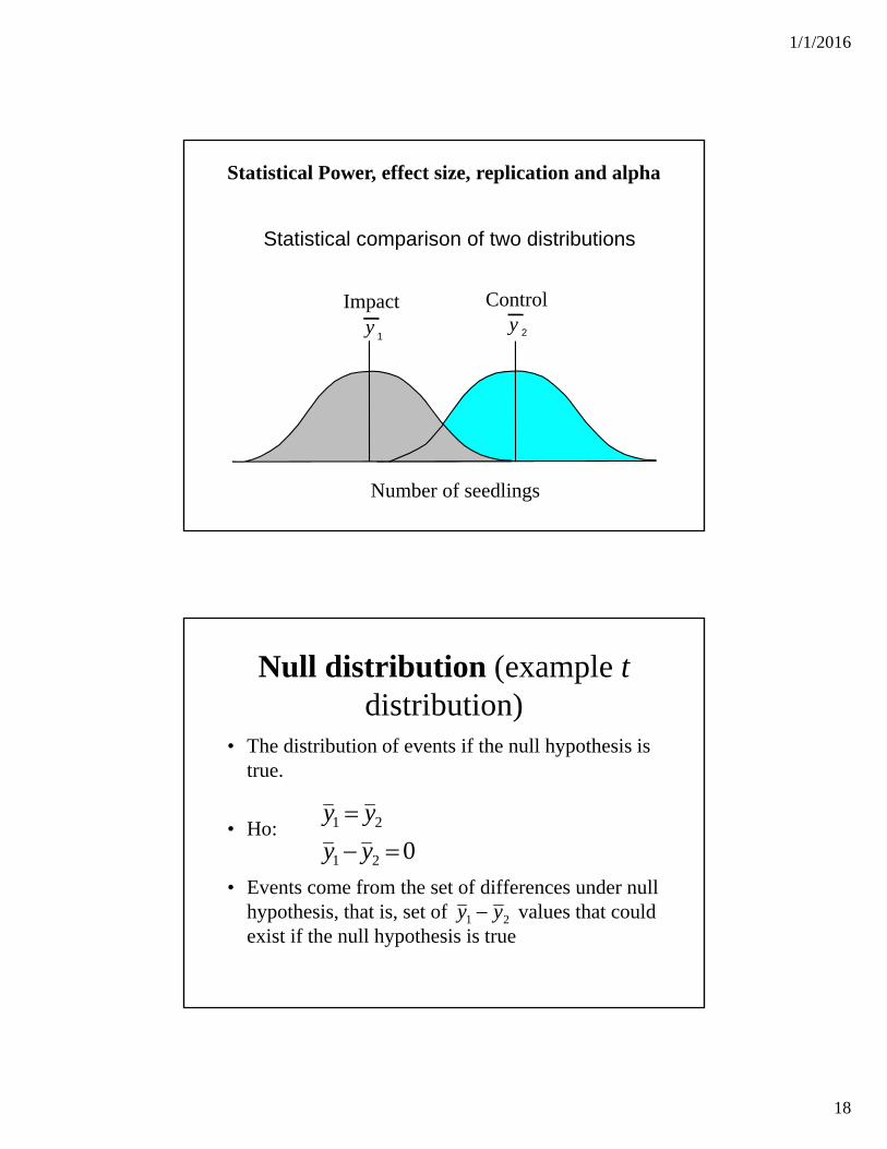
Statistical comparison of two distributions
Statistical Power, effect size, replication and alpha
Impact Control
Number of seedlings
Null distribution (example tdistribution)
• The distribution of events if the null hypothesis is true.
• Ho:
• Events come from the set of differences under null hypothesis, that is, set of values that could exist if the null hypothesis is true
021
21
yy
yy
21 yy

1/1/2016
19
t statistic – interpretation and units
• The deviation between means is expressed in terms of Standard error (i.e. Standard deviations of the sampling distribution)
• Hence the value of t’s are in standard errors
• For example t=2 indicates that the deviation (y1- y2) is equal to 2 x the standard error
ns /
y1 y2
-5 -4 -3 -2 -1 0 1 2 3 4 50.0
0.1
0.2
0.3
0.4
Pro
ba
bilit
y
ns /
y1 y2
Area under the curve = 1.00
Null distribution
Ho:
=y1 y2

1/1/2016
20
Components of the t equation-comparing two samples
y1 t =
y2
1
n1
1
n2
+sp
y1 t =
y2
1
n1
1
n2
+sp
Difference in the means of two samples
Pooled standard error=
1) Pooled standard error is an estimate of the error associated with the calculation of the difference between two sample means
2) Hence the t value increases with increasing difference between means and with decreasing standard error. The larger the value, the more confidence in concluding distributions (1 vs 2) are different
Ho true: Distributions of means are truly the same
Decision
Truth Accept HO Reject HO
HO true no error (1-alpha)
Type I error (alpha)
HO false Type II error (beta)
no error (1-beta)
central t distribution (df)
y1 t =
y2
1
n1
1
n2
+sp
y1 t =
y2
1
n1
1
n2
+sp
y1
y2
This is called the central t distribution – it is a null distribution
0t

1/1/2016
21
y1
y2
y1
y2
Ho true: Distributions of means are truly the same
y1 t =
y2
1
n1
1
n2
+sp
y1 t =
y2
1
n1
1
n2
+sp
-4 -3 -2 -1 0 1 2 3 4t - value
0
5
10
15
20
25
Cou
nt
0.0
0.1
0.2
Pro
po
rtion p
er B
ar
t distribution
20 25 30Mean Value from Sample
0
10
20
30
Co
un
t
0.0
0.1
0.2
0.3
Pro
po
rtion
pe
r Ba
r
20 25 30Mean Value from Sample
0
10
20
30
Co
un
t
0.0
0.1
0.2
0.3
Pro
po
rtion
pe
r Ba
r
(24.9 - 25.1)
Sample Means21.522.323.023.924.925.125.826.527.829.9
Impact
Ho true: Distributions of means are truly the same
Decision
Truth Accept HO Reject HO
HO true no error (1-alpha)
Type I error (alpha)
HO false Type II error (beta)
no error (1-beta)
Sample Means21.522.323.023.924.925.125.826.527.829.9
Control

1/1/2016
22
y1
y2
y1
y2
y1 t =
y2
1
n1
1
n2
+sp
y1 t =
y2
1
n1
1
n2
+sp
-4 -3 -2 -1 0 1 2 3 4t - value
0
5
10
15
20
25
Cou
nt
0.0
0.1
0.2
Pro
po
rtion p
er B
ar
t distribution
Ho true: Distributions of means are truly the same1) Estimate of y1 = estimate of y2
20 25 30Mean Value from Sample
0
10
20
30
Co
un
t
0.0
0.1
0.2
0.3
Pro
po
rtion
pe
r Ba
r
20 25 30Mean Value from Sample
0
10
20
30
Co
un
t
0.0
0.1
0.2
0.3
Pro
po
rtion
pe
r Ba
r
(24.9 - 25.1)
Sample Means21.522.323.023.924.925.125.826.527.829.9
Impact
Ho true: Distributions of means are truly the same
Decision
Truth Accept HO Reject HO
HO true no error (1-alpha)
Type I error (alpha)
HO false Type II error (beta)
no error (1-beta)
Sample Means21.522.323.023.924.925.125.826.527.829.9
Control

1/1/2016
23
y1
y2
y1
y2
y1 t =
y2
1
n1
1
n2
+sp
y1 t =
y2
1
n1
1
n2
+sp
-4 -3 -2 -1 0 1 2 3 4t - value
0
5
10
15
20
25
Cou
nt
0.0
0.1
0.2
Pro
po
rtion p
er B
ar
t distribution
Ho true: Distributions of means are truly the same2) Estimate of y1 = estimate of y2
20 25 30Mean Value from Sample
0
10
20
30
Co
un
t
0.0
0.1
0.2
0.3
Pro
po
rtion
pe
r Ba
r
20 25 30Mean Value from Sample
0
10
20
30
Co
un
t
0.0
0.1
0.2
0.3
Pro
po
rtion
pe
r Ba
r
(21.5 – 29.9)
t
assign critical p (assume = 0.05)
t c
Ho true: Distributions of means are truly the same
Decision
Truth Accept HO Reject HO
HO true no error (1-alpha)
Type I error (alpha)
HO false Type II error (beta)
no error (1-beta)
0
If distributions are truly the same then: area to right of critical t C
> t C will cause incorrect conclusion that distributions are different
represents the Type 1 error rate (Blue); any calculated t
central t distribution (df)y1
t =y2
1
n1
1
n2
+sp
y1 t =
y2
1
n1
1
n2
+sp

1/1/2016
24
0
t distribution (df)
y1 t =
y2
1
n1
1
n2
+sp
y1 t =
y2
1
n1
1
n2
+sp
Central t distribution
Non-central t distribution
Ho false: Distributions of means are truly different
t
y2y1
Ho false: Distributions of means are truly different
y1 t =
y2
1
n1
1
n2
+sp
y1 t =
y2
1
n1
1
n2
+sp
Mean value from sample
0
10
20
30
40
50
Co
un
t
0.0
0.1
0.2
0.3
0.4
0.5
Pro
po
rtion
pe
r Ba
r
Mean value from sample
0
10
20
30
40
50
Co
un
t
0.0
0.1
0.2
0.3
0.4
0.5
Pro
po
rtion
pe
r Ba
r
20 25 30
20 25 30
y2y1
-5 0 5
t - value
0
10
20
30
40
Cou
nt
0.0
0.1
0.2
0.3
0.4
Proportion per B
ar

1/1/2016
25
Ho false: Distributions of means are truly different
y1 t =
y2
1
n1
1
n2
+sp
y1 t =
y2
1
n1
1
n2
+sp
Mean value from sample
0
10
20
30
40
50
Co
un
t
0.0
0.1
0.2
0.3
0.4
0.5
Pro
po
rtion
pe
r Ba
r
Mean value from sample
0
10
20
30
40
50
Co
un
t
0.0
0.1
0.2
0.3
0.4
0.5
Pro
po
rtion
pe
r Ba
r
20 25 30
20 25 30
y2y1
-5 0 5
t - value
0
10
20
30
40
Cou
nt
0.0
0.1
0.2
0.3
0.4
Proportion per B
ar

1/1/2016
26
0
t distribution (df)
y1 t =
y2
1
n1
1
n2
+sp
y1 t =
y2
1
n1
1
n2
+sp
Central t distribution
Non-central t distribution
Ho false: Distributions of means are truly different
t
y1y2
assign critical p (assume = 0.05)
t c
Decision
Truth Accept HO Reject HO
HO true no error (1-alpha)
Type I error (alpha)
HO false Type II error (beta)
no error (1-beta)
Ho false: Distributions of means are truly different
If distributions are truly different then: area to left of critical t C
< t C will cause incorrect conclusion that distributions are same
represents the Type II error rate (Red); any Calculated t
0
t distribution (df)y1
t =y2
1
n1
1
n2
+sp
y1 t =
y2
1
n1
1
n2
+sp
Central t distribution
t

1/1/2016
27
0
t c
Type I errorType II error
Critical p
How to control Type II error (distributions are truly different)This will maximize statistical power to detect real impacts
1) Vary critical P-Values 2) Vary Magnitude of Effect3) Vary replication
Decision
Truth Accept HO Reject HO
HO true no error (1-alpha)
Type I error (alpha)
HO false Type II error (beta)
no error (1-beta)
Central t distribution
t
0
t c
Type I errorType II error
Critical p
How to control Type II error (distributions are truly different)
1) Vary critical P-Values (change blue area)
t c
Critical p
t c
Critical p
Reference
A) Make critical P morestringent (smaller)
A) Relax critical P (larger values)
Type II error increasesPower decreases
Type II error decreasePower increases
Decision
Truth Accept HO Reject HO
HO true no error (1-alpha)
Type I error (alpha)
HO false Type II error (beta)
no error (1-beta)
tt

1/1/2016
28
How to control Type II error (distributions are truly different) 2) Vary magnitude of effect (vary distance between y1 and y2, which affects non-central t distribution
9.5 10.5 11.5 12.5Mean value from sample
0
10
20
30
40
50
60
70C
oun
t
0.0
0.1
0.2
0.3
0.4
0.5
0.6
0.7
Prop
ortion p
er Bar
9.5 10.5 11.5 12.5Mean value from sample
0
10
20
30
40
50
60
Co
unt
0.0
0.1
0.2
0.3
0.4
0.5
0.6
Proportion per B
ar
9.5 10.5 11.5 12.5Mean value from sample
0
10
20
30
40
50
60
70
Cou
nt
0.0
0.1
0.2
0.3
0.4
0.5
0.6
0.7
Proportion
per B
ar
-5 0 5 10 15 20t value
0
10
20
30
40
50
60
Cou
nt
0.0
0.1
0.2
0.3
0.4
0.5
0.6
Pro
portio
n p
er B
ar
-5 0 5 10 15 20t value
0
10
20
30
40
50
60
Co
un
t
0.0
0.1
0.2
0.3
0.4
0.5
0.6
Pro
portio
n p
er B
ar
A.
B.
C.
B vs A
C vs A
y1 t =
y2
1
n1
1
n2
+sp
y1 t =
y2
1
n1
1
n2
+sp
y = 10
y = 10.5
y = 12
0
t c
Type I errorType II error
Critical p
t c
Reference
A) Make distance smaller
A) Make distance greater
Type II error increasesPower decreases
Type II error decreasesPower increases
0
t c
How to control Type II error (distributions are truly different)
Decision
Truth Accept HO Reject HO
HO true no error (1-alpha)
Type I error (alpha)
HO false Type II error (beta)
no error (1-beta)
0
2) Vary magnitude of effect (vary distance between y1 and y2, which affects non-central t distribution
tt
tt
tt

1/1/2016
29
How to control Type II error (distributions are truly different)
t c
Type I errorType II error
Critical p
Reference
A) Decrease replication
A) Increase replication
Type II error increasesPower decreases
Type II error decreasePower increases
t c
Decision
Truth Accept HO Reject HO
HO true no error (1-alpha)
Type I error (alpha)
HO false Type II error (beta)
no error (1-beta)
t c
3) Vary replication (which controls estimates of error)
- Note Type 1 error is constant and tc is allowed to vary
0
0
0
tt
tt
tt
T-test vs resampling
Test P-valueResampling 0.007T-test 0.019 Why the difference?
Pooled Variance
Variable Treatment Mean Difference
95.00% Confidence Interval
t df p-Value
Lower Limit Upper Limit
Number Inside -4.2 -7.49363 -0.90637 -2.94059 8 0.018693
Outside
Variable Treatment N Mean Standard
Deviation
Number Inside 5 5 2.54951
Outside 5 9.2 1.923538
Two-Sample t-Test
OutsideInside
Treatment
0123
Count
0
5
10
15
Num
ber
0 1 2 3
Count
0
5
10
15
Num
ber

1/1/2016
30
Replication and independence
Control sites Impact sites
Pseudoreplicationin space
Pseudoreplicationin time
Pseudoreplicationin time and space
Replication
Power
Low
High
Low High
Magnitude of Effect
Power
Low
High
Small Large
Critical alpha
Power
Low
High
Low High
POWER

1/1/2016
31
The fallacy of the primacy of alpha for environmental work
The trade-off between error and cost – an obvious conflict (I)
Sample size
Cos
t of
ass
essm
ent
Type I error, Power and experimental design
• Assume you want to know if discharge from a power plant affects rockfish density
• You want to be able to detect:– 20% difference in density
– Have power = 80% (0.8)
– Have critical alpha (Type 1 error) = 0.05
• You conduct a preliminary survey before you set up the experiment to estimate density– Now determine sample size necessary for your experiment
• Can it be done???

1/1/2016
32
Preliminary survey
Replicate Sample 1 Sample 21 3 62 9 93 18 134 15 85 10 126 8 157 15 98 7 109 6 13
10 11 7
Mean 10.2 10.2Standard Deviation 4.6 2.9
Probability (statistical) of detecting true impact
Cost of assessment
The fallacy of the primacy of alpha for environmental work
The trade-off between error and cost – an obvious conflict (II)
Probability (statistical) of concluding no impact
Therefore, the cynical conclusion is that the best strategy for anapplicant would be to under-fund an assessment
A) The lower the cost the more likely that a conclusionof no impact will be reached (regardless of the truth)

1/1/2016
33
The fallacy of the primacy of alpha for environmental work
The trade-off between error and cost – an obvious conflict (III)
Recommendations: 1) Determine the importance of error rates as a ratio
For example – what is the relative importance of:correctly concluding there is an impact (I) vs.correctly concluding there is no impact (N)
2) Determine the maximum Type 1 error acceptable (probability of concluding there is an effect (impact) when there is not one)
3) Estimate cost of assessment
4) Recycle procedure if necessary
5) Do not do the assessment if acceptable ratios and maximum error ratescannot be attained
General schematic for the design of a monitoring program1
Basic Sampling Design
Select Variables
Cost of errors
Refine design
Achievable?
Go
Effect Size Background Variation
Accept GreaterError Rate?
YY
N
1 from Keough and Mapstone 1993
N