The Livelihood and Poverty Mapping Analysis at Regional Level in

Pakistan

MSc Development Economics Thesis code: DEC 80433

By

Shazia Begum

Development Economics Group

Supervisor

Dr. Marrit van den Berg

August, 2015

i

Wageningen University and Research Centre

The Livelihood and Poverty Mapping Analysis at Regional

Level in Pakistan

Shazia Begum

751220-045-030 August, 2015

Supervisor WUR

Dr. Marrit van den Berg MSc International Development Studies

Specialization: Economics of Development

DEC-80433

ii

ACKNOWLEDGMENT

This research has been quite an exploratory event in my life that took me back to my home country.

Despite all the obstacles in the way I sailed through with the help of some of the most inspiring

personalities that I ever came across in my life during this research. Firstly, I must record my deep sense

of gratitude for my wur supervisor Dr. Marrit van den Berg for her guidance. Her supervision and timely

suggestions made it possible for me to complete this research work. I am also grateful to World Bank

Joint Japan Graduate Scholarship Program (JJ/WBGS) that financially supported me. Special

thanks for the co-operation of Pakistan Social Living Standard Measurement Survey Section of Pakistan

Bureau of Statistics for providing the datasets required for my research. It would be injustice if I do not

mention about my father, my sister, my brothers, and especially my deceased mother whose prayers still

overshadow in all the events of my life. Similarly, I am so very much indebted to my friends and fellow

colleagues, Rayke Berendsen , Pauline van Pommeren and Banchayehu Tessema Assefa for their

countless advices and suggestions without which the quality of this project as it is now would have been a

distant dream.

iii

Table of Contents

ACKNOWLEDGMENT .............................................................................................................. ii

List of Tables ................................................................................................................................. v

List of Figure ................................................................................................................................. v

ABSTRACT .................................................................................................................................. vi

1. Introduction ............................................................................................................................... 1

2. Conceptual framework ............................................................................................................. 4

2.1 The concept of wellbeing ................................................................................................... 4

2.2 Poverty Mapping ..................................................................................................................... 5

2.3 Conceptual framework for multidimensional poverty ........................................................ 7

3. Target Area................................................................................................................................ 8

3.1 Situation analysis for Pakistan ......................................................................................... 9

3.2 Situation analysis for Punjab Province ............................................................................ 9

3.3 Situation analysis for Sindh Province ............................................................................ 10

3.4 Situation analysis for KPK Province ............................................................................. 10

3.5 Situation analysis for Balochistan Province .................................................................. 11

4. Methodology and data ............................................................................................................ 12

4.1 Data ................................................................................................................................... 12

4.1.1 Description of HIES & PSLM ........................................................................................ 12

4.2 Model formation and SAE .............................................................................................. 13

4.3 Multidimensional Poverty ............................................................................................... 16

4.4 Poverty Maps .................................................................................................................... 20

5. Results and Discussions .......................................................................................................... 21

iv

5.1 Regression Analysis ......................................................................................................... 21

5.1.1 Household profile ............................................................................................................... 21

5.1.2 Household Head Characteristics ...................................................................................... 21

5.1.3 Household Welfare Characteristics................................................................................ 23

5.1.4 Assets ................................................................................................................................... 23

5.2 Uni-dimensional poverty across sub-regions of Provinces ................................................ 24

5.3 Multidimensional poverty across sub-regions of Provinces .............................................. 25

5.4 District/Division level Poverty Rates using simulated consumption .............................. 25

5.4.1 Punjab ............................................................................................................................... 26

5.4.2 Sindh.................................................................................................................................. 26

5.4.3 KPK ................................................................................................................................... 27

5.4.4 Balochistan........................................................................................................................ 27

5.4.5 Pakistan ............................................................................................................................. 28

5.5 Reliability of the maps .......................................................................................................... 33

6. Conclusion ............................................................................................................................... 34

6.1 Recommendations ................................................................................................................. 34

Bibliography ................................................................................................................................ 35

APPENDIX A .............................................................................................................................. 40

APPENDIX B .............................................................................................................................. 51

APPENDIX C .............................................................................................................................. 60

v

List of Tables

Table 4. 1: Coverage of Households in HIES & PSLM ........................................................... 13

Table 4. 2: Pearson Correlation Matrix .................................................................................... 14

Table 4. 3: Description of Covariates for consumption function............................................ 15

Table 4. 4: The cut-off point for each indicator of dimensions ............................................... 19

Table 4. 5: Weighting scheme for each dimension and indicator ........................................... 19

Table 5. 1: Punjab poverty estimates ........................................................................................ 29

Table 5. 2: Sindh poverty estimates........................................................................................... 30

Table 5. 3: KPK poverty estimates ............................................................................................ 31

Table 5. 4: Balochistan poverty estimates................................................................................. 32

Table 5. 5: Reliability Test ......................................................................................................... 33

List of Figure

Figure 2. 1: Development as good change from ill being to wellbeing ..................................... 5

Figure 2. 2: Pakistan Map ............................................................................................................ 8

Figure 4. 1: Dimensions for multidimensional poverty estimation ........................................ 18

Figure 5. 1: Poverty estimates - Uni-Dimensional…………………………………….……...24

Figure 5. 2: Multidimensional Poverty ..................................................................................... 25

vi

ABSTRACT

An attempt has been made to map the incidence of uni-dimensional and multi-dimensional poverty

simultaneously arguably for the first time in Pakistan. While multi-dimensional poverty map is calculated

using PSLM 2010-11; small area estimation technique is utilized to map uni-dimensional poverty using

both nationally representative HIES (Household Integrated Economic Survey) and district-level

representative PSLM (Pakistan Standard of Living Measurement) for the same year of 2010-11. The

result indicates the existence of spatial distribution of poverty pockets in each of the four provinces of

Pakistan. Furthermore, it is also observed that these pockets of poverty are more concentrated in the

desert and mountains regions of the country. Along with this, the poverty mapping exercise has shed light

on the fact that poverty has a negative feedback effect implying that underdevelopment breeds further

underdevelopment. Moreover, one overwhelming pattern observed is that extent of poverty exuberates

when attention is turned to multi-dimensional poverty from uni-dimensional poverty measure. This hints

towards a largely underdevelopment social sector in the country. However, as mentioned above, the

performance of the social sector also has a geographical character with Punjab having a relatively

stronger social sector track-record. Resultantly, Sindh, KPK, and Balochistan are lagging behind

drastically in terms of social sector performance. Subsequently, it is found that Balochistan and KPK are

the poorest regions multidimensionally along with Southern Sindh. In light of this, it is suggested that

nationally representative policies for poverty alleviation integrate need for geographical poverty

targeting.

Keywords: Poverty mapping, Small Area estimation technique, multi-dimensional poverty, spatial

distribution of poverty ,poverty alleviation.

1

Chapter 1

Introduction

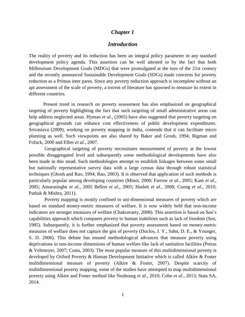
The reality of poverty and its reduction has been an integral policy parameter in any standard

development policy agenda. This assertion can be well attested to by the fact that both

Millennium Development Goals (MDGs) that were promulgated at the turn of the 21st century

and the recently announced Sustainable Development Goals (SDGs) made concerns for poverty

reduction as a Primus inter pares. Since any poverty reduction approach is incomplete without an

apt assessment of the scale of poverty, a torrent of literature has spawned to measure its extent in

different countries.

Present trend in research on poverty assessment has also emphasized on geographical

targeting of poverty highlighting the fact that such targeting of small administrative areas can

help address neglected areas. Hyman et al., (2005) have also suggested that poverty targeting on

geographical grounds can enhance cost effectiveness of public development expenditures.

Srivastava (2009), working on poverty mapping in India, contends that it can facilitate micro

planning as well. Such viewpoints are also shared by Baker and Grosh, 1994; Bigman and

Fofack, 2000 and Elber et al., 2007.

Geographical targeting of poverty necessitates measurement of poverty at the lowest

possible disaggregated level and subsequently some methodological developments have also

been made in this stead. Such methodologies attempt to establish linkages between some small

but nationally representative survey data with a large census data through robust statistical

techniques (Ghosh and Rao, 1994; Rao, 2003). It is observed that application of such methods is

particularly popular among developing countries (Minot, 2000; Farrow et al., 2005; Kam et al.,

2005; Amarasinghe et al., 2005 Bellon et al., 2005; Haslett et al., 2008; Cuong et al., 2010;

Pathak & Mishra, 2011).

Poverty mapping is mostly confined to uni-dimensional measures of poverty which are

based on standard money-metric measures of welfare. It is now widely held that non-income

indicators are stronger measures of welfare (Chakravarty, 2008). This assertion is based on Sen’s

capabilities approach which compares poverty to human inabilities such as lack of freedom (Sen,

1985). Subsequently, it is further emphasized that poverty assessment based on money-metric

measures of welfare does not capture the gist of poverty (Duclos, J. Y., Sahn, D. E., & Younger,

S. D. 2006). This debate has ensued methodological advances that measure poverty using

deprivations in non-income dimensions of human welfare like lack of sanitation facilities (Petras

& Veltmeyer, 2007; Costa, 2003). The most popular measure of this multidimensional poverty is

developed by Oxford Poverty & Human Development Initiative which is called Alkire & Foster

multidimensional measure of poverty (Alkire & Foster, 2007). Despite scarcity of

multidimensional poverty mapping, some of the studies have attempted to map multidimensional

poverty using Alkire and Foster method like Neubourg et al., 2010; Cobo et al., 2013; Stats SA,

2014.

2

In Pakistan’s perspective, the poverty reduction policies have usually recorded lackluster

performance. It is observed that such policies in Pakistan are marked by disregard for spatial

distribution of poverty. Arif (2012) evaluating Pakistan poverty reduction strategies historically

in the context of China’s experiment with poverty reduction also substantiate this argument

stating that “no attempt has, so far, been made to target poor regions for development and

poverty reduction”. IMF (2013) also mentions the fact that some of poverty reduction strategy

tools like micro credit is also not extended keeping in mind the geographical pockets of poverty

in Pakistan. This, however, is not hard to understand, since the poverty assessment literature in

Pakistan has not disaggregated poverty measures at the lowest possible level on consistent basis.

There are few exceptions to this case. Jamal (2007) combined HIES 2004-05 and PSLM

2004-05 using small area estimation technique for the first time in the country to measure the

incidence of poverty among all the districts of Pakistan’s provinces. However, Jamal (2007)

failed to paint a clear picture of poverty spread across the country as it only concluded that rural

Balochistan and small towns or cities are most vulnerable. Furthermore, it is also observed that

Small Area Estimation technique is not used in its true spirit in this study since it does not

calculate probabilities by using standard error to obtain district level poverty estimates. Davis

(2003) outlines at length that standard errors are used to calculate sub-regional poverty

incidence. Jamal (2013) updated his previous estimates using nationally representative HIES

2010-11 survey and district-level representative PSLM 2010-11. However, the same

methodological pitfalls are retained in this study as well. Another drawback noted is that both of

these studies models consumption expenditure at rural and urban level only despite the fact that

HIES survey data in Pakistan is representative at provincial level. Similarly, Cheema et al.,

(2008) using Multiple Indicators Cluster Survey (2003-2004) mapped poverty incidence for

Punjab province only. Said et al., (2011) disaggregated poverty at district level using PSLM

2008-09 through Asset Index and Basic Need Index. Burki et al., (2015) also used asset index to

map poverty but only in case of Punjab. In the same vein, Naveed & Ali (2012) mapped

multidimensional poverty in districts of Pakistan using PSLM 2008-09. While Jamal (2012)

estimated district level multidimensional poverty estimates using Alkire and Foster method but

its choice of dimensional indicators seems arbitrarily and not based on any specified reference

like MDGs.

In the context of these limitations noted in the literature internationally and nationally in

Pakistan, the present study attempts to bridge these gaps by first updating the multidimensional

poverty maps for each province of Pakistan and for Pakistan as a whole at district level using

latest available data of PSLM 2010-11 and adopting Alkire and Foster method. It must be noted

here that choice of dimensional indicators and their respective cut-offs points are compared to

and based on the Sustainable Development Goals mostly while partial comparison is also made

to Millennium Development Goals. Uni-dimensional maps of poverty are also made using Small

Area Estimation. The district level estimates for each district of Pakistan are calculated by fitting

consumption model for each of the four provinces of the country along with incorporating

3

standard error in calculating probability of being poor. Finally, in contrast to other studies in

Pakistan the present study also estimates poverty at divisional level. Moreover, the present study

is arguably first of its kind in Pakistan that maps both uni-dimensional and multi-dimensional

poverty estimates at district level for each province and Pakistan as a whole simultaneously. It is

expected that this study can contribute in enhancing the understanding regarding the spatial

distribution of poverty and hence, may facilitate in geographical poverty targeting in Pakistan.

The study can also highlight districts in which social sector requires attention of policy makers

and districts in which standard income-promoting measures can stand in good stead. It is

contended that in this way social dividend of national policies can be increased. The pertinent

research objectives are delineated as hereunder:

1. To map the multidimensional and uni-dimensional poverty of the four provinces of

Pakistan i.e. Punjab, Sindh, Khyber Pakhtoonkhwa and Baluchistan at division and

district level.

2. To compare the multidimensional poverty index to uni-dimensional poverty in each

district and division of Punjab, Sindh, Khyber Pakhtoonkhwa and Baluchistan.

The report is divided into five chapters. Second chapter covers the conceptual framework of the

study while third chapter elaborates in detail the methodology used for analysis. Fourth chapter

explains the empirical results of the study and the final section concludes.

4

Chapter 2

Conceptual framework

This chapter tackles the conceptual building blocks on which the ensuing chapter of

methodology is based. Since, the study also measures multidimensional poverty which relies on

non-income approach to welfare section 2.1 presents a detailed discussion on wellbeing.

Similarly, section 2.2 presents the framework of small area estimation while the final section 2.3

covers Alkire and Foster measure which is used for multidimensional poverty calculation.

2.1 The concept of wellbeing

World Bank (2000) relates poverty to well-being in the most succinct way by regarding

deprivation in well-being as poverty. The subsequent question that hails from this is what

constitutes well-being (Haughton & Khandker, 2009). The conventional answer revolves around

control-over-commodities/resources argument which subsequently uses monetary indicators like

income or consumption expenditure as a proxy of well-being. This argument is further based on

the pretext that most of the non-income indicators like health, education, and assets etc. are

positively correlated with income (Bourguignon & Chakravarty, 2002). However, Sen (1987)

augments this parochial argument by defining well-being in a broader sense relating it to

functional capability of any individual in a society. Based on this, in spite of income well above

poverty line an individual can be poor if he can’t discharge basic functioning in a society due to

certain incapability’s like lack of education or health. Hence, poverty is regarded as a state of

impotency.

Some other studies like Ravallion & Chen, 1994; Bourguignon & Chakravarty, 2003;

Caroline, 2003; and Maltzahn and Durrhiem ,( 2008) also criticize income as a measure of well-

being in poverty measurement. Sen (1985, 1987, 1992, 1993, 1994, and 1997) distinguishes

between commodities, human functioning/ capability and utility as follows:

Commodity Capability (to function) Function(ing) Utility (e.g.

happiness).

Sen(1992) says commodities are the goods and services that can be used for functioning while

capabilities relate to the functions and freedom of choice of living. Such deprivations can be

lack of food, housing, education, and health facilities, land, etc.

.

5

Figure 2. 1: Development as good change from ill being to wellbeing1

2.2 Poverty Mapping

In monitoring the performance of different countries towards MDGs, World Bank relied on

poverty mapping approach using income-poverty as the measure of poverty. Nevertheless,

poverty mapping is not only restricted to income-poverty mapping and can be categories into

four major groups.

Economic. Monetary indicators of the well-being of the household which include

consumption and non-consumption expenditure and the household income. These

measures are mostly used for the poverty analysis. The well being is also analyzed by

taking the non-monetary proxies such as the productive household assets.

Social. Other none-monetary indicators of the household like the access of quality of

education, health, basic needs of life etc.

Demographic. The demographic indicators of the household like the age, gender,

household size etc.

Vulnerability. This include the capability of household to shocks that can affect the

livelihood such as the food insecurity ,political stability, environmental change and the

alternatives of the livelihood etc

Such techniques estimate poverty at “small area” levels representing subset of a larger

population. The term small area refers to small geographical units such as districts and

municipalities. Census usually provides limited information on required variables and the survey

data usually have the coverage problem. The “direct method” to measure such estimates is based

on some national survey data. However, such approaches eventuates poverty measures with large

standard errors and hence, are unreliable. This is overcome by the so-called “indirect method” of

small area estimation which enhances the reliability of the poverty estimates by linking the

variable of interest with a large census data through a model (Ghosh & Rao, 1994; Rao 1994;

1 1 Poverty in Focus, International Poverty Centre United Nations Development Programme , December ,2006

6

Rao, 2003; and Jiang and Lahiri, 2006). These methods are model-based and have been well

developed in the literature (Marker, 1999 and Noble et al., 2002; Elbers et al., 2003).

Small area estimation is one of the techniques for poverty mapping. This technique

requires two datasets; one is used to estimate the function of the target variable while the other

data set is used to estimate the target variable among a larger proportion of the population. The

first step is to estimate the model statistically representative at regional level with explanatory

variables common in both data sets. The following equation is estimated using the ordinary least

square.

ln(𝐶) = 𝛼 + 𝛽1𝑋 + 𝛽2𝑉 + 𝜀 (1)

Where the C is the per-adult consumption, X is the vector of household level characteristics and

V is the geographical characteristics.

𝐹𝑖𝑗 = 1 𝑖𝑓 𝑙𝑛𝐶𝑖𝑗 < 𝑙𝑛𝑧; (2)

𝐹𝑖𝑗 = 0 𝑜𝑡ℎ𝑒𝑟𝑤𝑖𝑠𝑒

Where F in equation (2) above nominates a household poor or non-poor, if its per capita adult

equivalent consumption expenditure is below or above the poverty line z respectively. Following

Hentschel et al., (2000), household level explanatory variables are multiplied by the

corresponding parameter estimate i.e.𝛽𝑖 for each ith variable obtained from the equation (1). This

gives the simulated log of per capita adult equivalent consumption expenditures for each

household in the census data. The estimated value of indicator, represented by 𝑋𝑖′𝛽 in equation

(3), is used to be determining the probability of a household being poor in terms of a given

threshold based on per capita adult equivalent consumption.

𝐸 (𝐹𝑖

𝑋𝑖, 𝛽, 𝜎) = ∅ [

𝑙𝑛𝑧−𝑋𝑖′𝛽

�̂�] 2 (3)

Where ∅ the standard normal distribution and z is poverty line in money metric units. Similarly,

𝛽 is the vector covariates while �̂� is the estimated error from the model in equation 1. This

equation gives the probability that a household is poor.

𝐹𝑖∗ = 𝐸 (

𝐹𝑖

𝑋𝑖= 𝑖, �̂�, �̂�) = ∅ [

𝑙𝑛𝑧−𝑋𝑖′�̂�

�̂�] (4)

Regional poverty, F is found with

𝐹 = 1

𝑁∑ 𝐹𝑖

𝑁𝑖=1 (5)

N is the number of household in the specific region. Expected poverty is found with:

2 Davis, B. (2003). Choosing a method for poverty mapping. Food & Agriculture Org.

7

𝐸 (𝐹

𝑋, 𝛽, 𝜎) =

1

𝑁∑ 𝐸 (

𝐹𝐼

𝑋𝑖, 𝛽, 𝜎)𝑁

𝑖=1 (6)

The mean probability of households being poor is calculated as:

𝐹∗ = 𝐸 (𝐹

𝑋, 𝛽,̂ �̂�) =

1

𝑁∑ ∅𝑁

𝑖=1 [𝑙𝑛𝑧−𝑋𝑖

′�̂�

�̂�] (7)

2.3 Conceptual framework for multidimensional poverty

In the present multidimensional poverty is assessed using Alkire and Foster methodology. The

method is based on two steps only i.e. aggregation and identification. The aggregation steps

involve how seemingly different indicators measured in different units are aggregated. This step

is accomplished using matrix y of list of indicators as the one mentioned hereunder. Where 𝑦1𝑗

means j indicator of human welfare for household 1 and 𝑦1𝑐 means that observations from

household 1 is taken for upto c indicators. Similarly, observations are taken from n households

on indicators j to c. These indicators of welfare may be years of schooling or access to some

facility like health.

𝑦 = [

𝑦1𝑗 ⋯ 𝑦1𝑐

⋮ ⋱ ⋮𝑦𝑛𝑗 ⋯ 𝑦𝑛𝑐

]

𝑧 = [𝑧𝑗 … 𝑧𝑐]

Furthermore, depending on the specified poverty line or cut-off point for each indicator labeled zj

in the above row-vector z a censored matrix is obtained. Matrix z is the vector of such cutoff

points. As for censored matrix it is measured by replacing 1 against each household who is

deprived in any indicator while non-deprived household are coded as 0. It is denoted by g0 of

zeros and ones and looks like following:

𝑔0 = [1 1 00 0 11 0 1

]

The ones and zeroes are entered in this case just to show how it looks like. Row-wise additive

operation is carried out on this matrix to obtain another vector c which shows the sum of

indicators in which a certain household is deprived. Henceforth, using dual cutoff point which

assigns a value to k that is less than total number of indicators households are further screened

that are below this value of k as only those households are retained with non-zero value that has

an aggregated sum of deprived well over or equal to k. The column vector c is now label as c(k).

This vector is further divided by the number of total indicators and averaged across each

household to get average deprivation A which is then multiplied by headcount ratio H to estimate

adjusted headcount M(z,y).

8

Chapter 3

Target Area

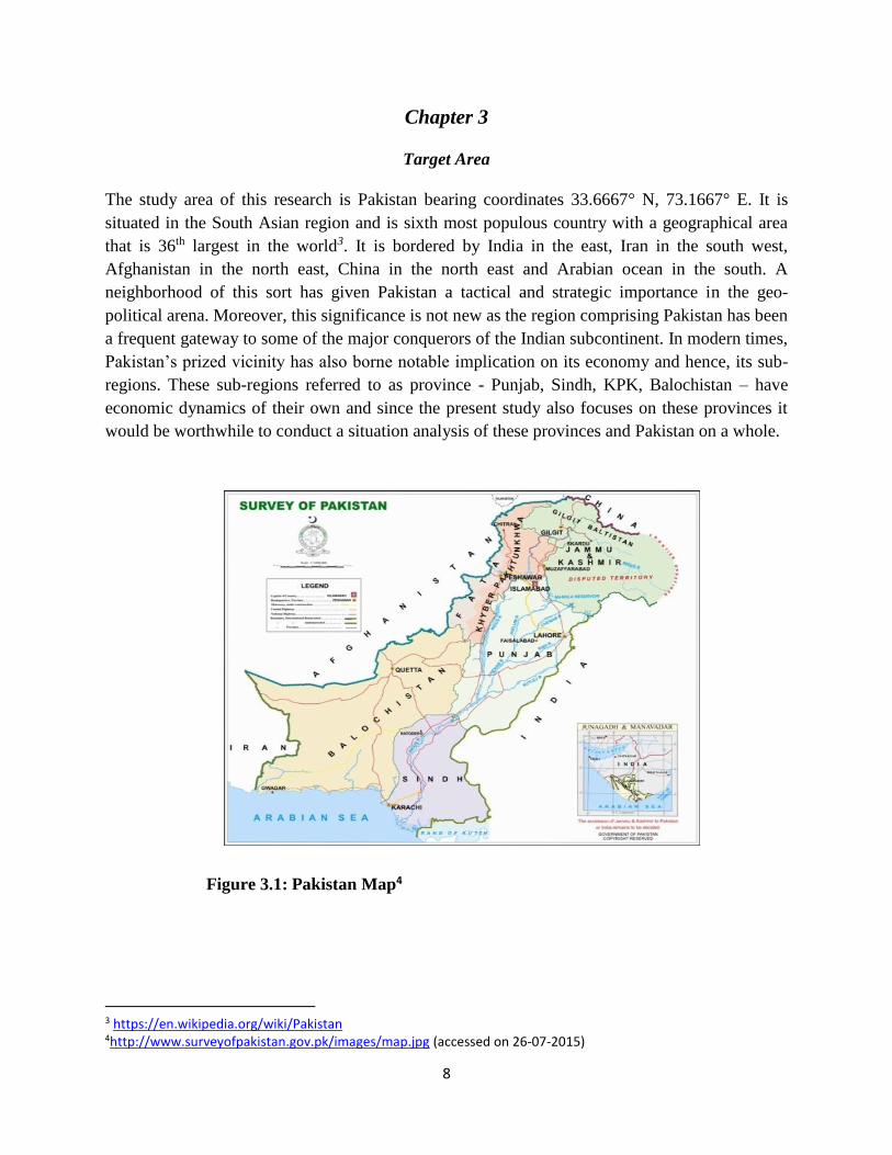
The study area of this research is Pakistan bearing coordinates 33.6667° N, 73.1667° E. It is

situated in the South Asian region and is sixth most populous country with a geographical area

that is 36th largest in the world3. It is bordered by India in the east, Iran in the south west,

Afghanistan in the north east, China in the north east and Arabian ocean in the south. A

neighborhood of this sort has given Pakistan a tactical and strategic importance in the geo-

political arena. Moreover, this significance is not new as the region comprising Pakistan has been

a frequent gateway to some of the major conquerors of the Indian subcontinent. In modern times,

Pakistan’s prized vicinity has also borne notable implication on its economy and hence, its sub-

regions. These sub-regions referred to as province - Punjab, Sindh, KPK, Balochistan – have

economic dynamics of their own and since the present study also focuses on these provinces it

would be worthwhile to conduct a situation analysis of these provinces and Pakistan on a whole.

Figure 3.1: Pakistan Map4

3 https://en.wikipedia.org/wiki/Pakistan 4http://www.surveyofpakistan.gov.pk/images/map.jpg (accessed on 26-07-2015)

9

3.1 Situation analysis for Pakistan

The socio-economic realities of Pakistan have undergone drastic changes since its inception in

1947. However, it is observed that some have been incessant. One of these is that agriculture still

retains its significance in the socio-economic life of the people of Pakistan. While its share in

GDP is no longer what it was four decades ago it still is the largest employer of labor force in the

country. However, other sectors like manufacturing and particularly services have witnessed

marked improvements. These changes installed Pakistan on a growth trajectory that has

established Pakistan as the one of the Next Eleven economies earmarked by Goldman Sachs as

the ones having most potential to be among world’s largest economies5. However, the recent

macro challenges like energy shortages, corruption, and poor performing public services like

train transportation have dinted the economy and intercepted its growth trajectory. Along with

this, Pakistan has also borne its share of shocks like terrorism and floods. It must be noted here

that specter of political instability has been a recurrent problem of Pakistan, so much so, that

despite being its more than a half century of history, Pakistan still remains a nascent democracy.

Such trends have resulted in weak institutions which perpetuate the already entrenched nuisance

of rent seeking. All of these factors have resulted in a high incidence of poverty in the country.

By one measure, using a benchmark of 2 dollars a day, about two-thirds of the population is

stuck in poverty6.

3.2 Situation analysis for Punjab Province

Punjab is Pakistan’s bread basket catering for a better share of the population of the country.

This mainly is a result of well-irrigated landscape of the province. Moreover, its cash crops like

wheat, cotton and sugarcane Along with this, Punjab is also the major contributor to the national

pool of professionals as well as technical man power. Punjab is the most populated province of

the country with 56 percent of the total national population living in it (Livingston and

O’Hanlon, 2011). Punjab’s share in the economic pie of the country is 57 percent of gross

domestic product in the year 2010 up marginally from 54.7 percent in 20007. This marginal

increase can be attributed to the massive power crisis that rocked the nation during the late 2000s

and still persists at the time of writing and is assuming significance of mammoth proportions.

One estimate claims that this energy crisis cost Punjab 2 to 3 percent of GDP8. Resultantly, the

income per capita in the province also declined which is also the second largest in the country

behind Sindh9. Similarly, floods, poor agriculture performance and terrorism remain some the

5 Goldmand Sach’s MIST Toppling BRICs as Smaller Market Outperforms. http://www.bloomberg.com/news/articles/2012-08-07/goldman-sachs-s-mist-topping-brics-as-smaller-markets-outperform 6 Where population growth poses the greatest challenge. https://www.populationinstitute.org/external/Final-DVI-report.pdf 7 Punjab’s lost growth momentum. http://www.dawn.com/news/719999/punjabs-lost-growth-momentum 8 Punjab’s economic performance. http://tribune.com.pk/story/436058/punjabs-economic-performance/ 9 Punjab’s economic importance. http://tribune.com.pk/story/378252/punjabs-economic-importance/

10

major challenges facing the economy of Punjab. Nevertheless, Punjab remains the most

industrial area of the country with sub-regions noted for production of sports and surgical

instruments like Sialkot, IT production like Lahore and textile production in case of Faisalabad.

3.3 Situation analysis for Sindh Province

The economy of Sindh is geared mostly by Karachi which is sole operative coastline of the

country while partial contribution from Hyderabad is also noted. One the major reason for

reliance on Karachi is due to the fact a better part of the province is covered by the notorious

desert of Thar which is the 17th largest in the world. In spite of this, agriculture is an important

part of the province with cotton, rice, wheat, sugar cane, bananas, and mangoes being some of

the major crops in the region. However, Sindh’s main economic challenge is that of a lagging

social sector which is exuberated by the political instability in the province especially Karachi.

Sindh is marked by low enrollment rate of children aged 4-9, a high infant mortality rate of 95

per 1000 births, and only 10 percent of rural areas have access to potable water10. A major point

of concern is the problem of social instability as events of sectarian and religious clashes have

frequent marred and dented the performance of the country.

3.4 Situation analysis for KPK Province

KPK is home to the oldest city in South Asia i.e. Peshawar, and its Khyber Pass has witnessed

rumbling sounds of armies arguably more than any other city in South Asia. As a result, the

people of the region have assumed a warlike demeanor clouded behind the cover of

conservatism. Its proximity with Afghanistan which has been the centre of geo-political show-

down since the invasion of Soviet Union has caused unprecedented damage to its economy.

Terrorism and militancy is so much embedded in the province that despite being accounting for

13.7 percent of the nation’s population, it only contributes 8 percent to its GDP11. KPK’s

situation as of late has turned into a fiscal crisis of its own because the brunt of military response

to militancy has been borne by provincial and national exchequer12. Subsequently, this comprises

the efforts of the province to reinvigorate to an already poor side of its social sector performance

especially in health sector. So much so, that as per World Health Organization, Peshawar which

is the capital of the province is the world’s largest reservoir of Polio13.

10 Sindh’s Development: Issues and Agenda. http://siteresources.worldbank.org/PAKISTANEXTN/Resources/Pakistan-Development-Forum/Sindh.pdf 11 Economics and extremism. http://www.dawn.com/news/844412/economics-and-extremism 12 Pakistan’s Taliban fight threatens key economic zone. http://www.wsj.com/articles/SB124237648756523343 13 WHO declares Peshawar world’s largest reservoir of Polio. http://www.dawn.com/news/1080926

11

3.5 Situation analysis for Balochistan Province

Balochistan has become synonyms with underdevelopment and natural gas in the context of

Pakistan. Separatist movements in the province are active. As a result of this, efforts to tap into

the province’s resource base have been undermined. This is well gauged by the fact that the

installation of Gwadar port – which will be the largest of the country – didn’t start until 2000s.

Among other resources present in the province are coal, copper, lead, gold, and other minerals.

As in case of KPK, Balochistan’s social sector is well below the acceptable limits of human

development. Along of this, some of the major challenges facing the province are: 1) low

growth; 2) low urbanization; 3) low labor productivity; 4) low quality jobs; 5) high population

growth; and 6) gender-gaps14. However, as in case of other provinces of the country, agriculture

and livestock sector are dominant in the province.

14 Pakistan Balochistan Economic Report. http://siteresources.worldbank.org/PAKISTANEXTN/Resources/293051-1241610364594/6097548-1257441952102/balochistaneconomicreportvol2.pdf

12

Chapter 4

Methodology and data

This chapter outlines the procedures related to the application of small area estimation and

multidimensional poverty estimation in case of Pakistan. Data description is chalked in section

3.1. Section 3.2 deals with model formation and also outlines how small area estimation

technique is conducted in the context of the present study for calculating poverty at division and

district level. Section 3.3 provides information on how Alkire and Foster method for

multidimensional poverty estimation is carried out using PSLM data for the year 2010-11.

Finally, section 3.4 covers how estimated disaggregated poverty measures are displayed on

maps.

4.1 Data

The SAE is implemented on Pakistan’s Household Integrated Economic Survey (HIES) which is

representative at national and provincial level and Pakistan Social and Living Standards

Measurement (PSLM) data which is representative at district level. These datasets are taken for

the same year of 2010-11 both of which were complied by Pakistan Bureau of Statistics (PBS).

HIES basically covers the income and expenditure profile while PSLM focuses more on social

facets of households.

4.1.1 Description of HIES & PSLM

The Household Integrated and Economic Survey (HIES) was conducted in 1963 and since then it

has been issued irregularly. HIES is representative at provincial and national level. The data

collection technique employed is two-stage stratified random sampling with all urban and rural

areas constitute the universe apart from military restricted areas. The sampling frame in case of

urban areas consists of enumeration blocks that includes cities and towns with about 200-250

households in each enumeration block. These enumeration blocks are further divided into low,

middle, and high income categories. It must be mentioned here that cities with population greater

than or equal to half of a million are considered an independent stratum while the other small

urban areas are clustered together into an independent stratum. However, contrary to this each

village is regarded as an independent stratum in case of rural areas. This, however, is not so in

case of Baluchistan where administrative divisions are regarded as stratum. Subsequently, as for

urban areas from each stratum enumeration blocks are randomly selected which are called

primary sampling units. Furthermore, households are picked from each sampled PSUs. The

households are treated as Secondary Sampling Units (SSUs).In urban area 12 and in rural areas

16; SSUs are selected by systematic sampling technique. As for PSLM, all the details from

enumeration blocks in urban areas to sampling technique used are same as that in HIES.

However, the only difference is in how strata are defined. In case of PSLM, apart from large

cities like Islamabad, Lahore, Gujranwala, Faisalabad, Rawalpindi, Multan, Bahawalpur,

13

Sargodha, Sialkot, Karachi, Hyderabad, Sukkur, Peshawar, and Quetta all the other urban

districts are considered as independent stratum. While the same also goes for rural districts. This

is in contrast to HIES, where large cities and clustered of small cities/towns are bundled to from

stratums and villages are deemed as stratum in case of rural areas. Hence, the number of sampled

households as a result of this procedure in HIES and PSLM are shown in table 4.1.

As for coverage, the major purpose for the HIES survey was to chart the economic

aspects of households which are incorporated in its consumption module. In this way, HIES is

mostly used in ascertainment of monetary poverty in the country. However, information of

demographics, education, health, and employment/income are also collected. On the other hand,

assessment of social sector performance in the country is the main reason for compiling PSLM

and hence, calculation of non-income poverty is one of the major uses of this data.

Table 4. 1: Coverage of Households in HIES & PSLM

HIES PSLM

Province PSUs SSUs PSUs SSUs

Punjab 512 6952 2344 32380

Sindh 296 4097 1407 19622

KPK 208 2954 849 12479

Balochistan 164 2335 813 12065

Total 1180 16338 5413 76546

Source: PSLM, 2010-11

4.2 Model formation and SAE

This section deals with the specification of the consumption model outlined in chapter 2 in the

context of the present study. The set of explanatory variables belong to varied categories and

represent households-level characteristics along with some characteristics pertinent to household

head. Moreover, some of the covariates are also selected as auxiliary or control variables. The

choice of these variables is not arbitrary and hails directly from the review of literature on

modeling of consumption function based on survey data (Parker, 1999; Filmer, 2000; Jayaraman

and Findeis, 2005; Chaudhry & Rehman, 2009; Fidrmuc & Senaj, 2012; Moaz & Neeman, 2008;

Sewanyana, 2009; Kudebayeva and Barrientos, 2013.

The list of covariates is tabulated in table 4.3 along with their detailed description. Furthermore,

unless otherwise stated, no serious correlation is found between the covariates that are

continuous. This is adjudged by using Pearson correlation matrix which measures correlation

among continuous variables only. The results of this matrix are presented in table 4.2. Since

consumption function is estimated on survey data of HIES, the selected correlates are picked

from different sections of HIES survey and merged to form one independent file to enhance

operation convenience. The STATA do-file used to serve this purpose is illustrated in Appendix

B.1. It is noted here that this do-file is also valid for PSLM since definitions as well as names of

relevant variables and their respective files are consistent with that of HIES.

As for the dependent variable, consumption expenditure per adult equivalent is used. The

rationale for using adult equivalent consumption is that members of a household with different

14

ages have different consumption requirements while the reason for opting for consumption

expenditure is that consumption expenditure are deemed more reliable than income estimates

especially in case of developing countries which are marked by a dominant agriculture sector.

Haughton and Khandker (2009) also emphasis the invalidity of income estimates noting that

capital gains which constitute income measurement like increase in the worth of fixed assets and

farm animals are difficult to calculate. In calculation of consumption, expenditure on food items

and non-durable goods and services are used. Appendix B.2 presents the STATA do-file for

aggregation of these consumption components and appendix B.3 constitutes do-file for

calculating household size by incorporating the economies of scale in consumption expenditure

among household’s members. It also shows how adult equivalent consumption expenditure is

calculated and merged with datasheet of covariates complied earlier. Furthermore, the dependent

variable is transformed into log scales and subsequently merged with covariates file to set up the

final file on which log-linear consumption model is estimated as specified in equation 1 in

chapter 2.

Having finalized the covariates and the consumption expenditure per adult equivalent, survey

regression is used to estimate equation 1 in chapter 2 with the aim to account for the weighting

structure of HIES for each province. Moreover, robust standard errors of beta coefficients are

used and no additional command has to be specified for it since; survey regression in STATA

displays robust standard errors for estimated beta coefficients by default. This constitutes the first

step in Small Area Estimation. As standard error of the model is used to estimate poverty

incidence at district and division level it is noted that survey regression in STATA does not

calculates standard error of the model. Subsequently, this non-availability is overcome by

calculating standard error of the model for each log-liner consumption equation i.e. for each

province. In the second step, the beta coefficients thus obtained are interpolated to district sheet

of variables to simulate consumption expenditure at district as well as division level which forms

the second step of the method. In contrast to other studies in Pakistan, standard errors are used to

first find z-scores for each household which are then used to calculate probability of being

poverty of each household using STATA normal function. These probabilities are found using

equation 4 in chapter 2 where z i.e. the poverty line is the official poverty line Rs. 1745 for the

understudy year 2010-11 (PBS, 2014).

Table 4. 2: Pearson Correlation Matrix

HH size Proportion of

adults

Proportion of

females

Proportion

of children

Assets No of

rooms

Age

HH size 1

Proportion of adults -0.1095 1

Proportion of

females

-0.0083 0.0586 1

Proportion of

children

0.27 -0.2062 0.0568 1

Assets 0.1061 -0.0028 0.025 -0.1986 1

No of rooms 0.3337 0.0432 0.0014 -0.1382 0.4537 1

Age 0.1866 0.3681 -0.0474 -0.3709 0.1569 0.2463 1

Source: Author’s Calculation using PSLM 2010-11

15

Table 4. 3: Description of Covariates for consumption function

Category Variable Variable type

Household

Profile

Household size Continuous

Proportion female (fraction) Continuous

Proportion of children Continuous

Proportion of adults Continuous

Household

head

characteristics

Head no spouse

Head is female

Age of household head.

Education of household head

Dummy Variable

Widow/Unmarried/Head=1

Otherwise = 0

Dummy Variable

Female = 1

Male = 0

Continuous

Categorical Variable

Illiterate = 1

Primary Education =2

Secondary Education = 3

Degree education = 4

Type of employment of household head Categorical Variable

1. Not employed

2. Head has employed < 10

3. Head has employed >10.

4. Head is self employed.

5. Paid employee.

6. Unpaid family worker

7. Head is own cultivator.

8. Head is share cropper.

9. Head is contract cultivator.

Household

characteristics

Household

Characteristics

House ownership status Dummy Variable

Personal residence (hired or not hired), without rent.

(not-deprived) = 1

Deprived otherwise = 0

Source of fuel Dummy Variable

Firewood, Sticks, Coal, and Wooden Coal dung

cake (Deprived) = 0

Gas, Kerosene oil and electricity (Not deprived)= 1

Variable Variable Type

Source of lighting Dummy Variable

Electricity, gas, kerosene oil (not deprived) = 1

Otherwise deprived = 0

Source of drinking water Dummy Variable

Open well, river, tanker, and others (deprived) = 0

Open well, river, tanker, mineral water = 1

Type of toilet Dummy Variable

Digged ditched, Flush system connected to

sewerage, flush system connected to septic tank.

(not deprived) = 0

Otherwise deprived = 1

Type of roof Dummy Variable

RCC/RBC, iron & cement (not-deprived) = 1

Deprived Otherwise = 0

Number of rooms Continuous

16

Category Variable Variable type

Assets Household has the Agriculture land

Household has livestock

Dummy Variable

Yes = 1

No = 0

Dummy Variable

Yes = 1

No = 0

Household has car Dummy Variable

Yes = 1

No = 0

Household the television Dummy Variable

Yes = 1

No = 0

Household has Refrigerator Dummy Variable

Yes = 1

No = 0

Household has Motorcycle. Dummy Variable

Yes = 1

No = 0

Household has A/C Dummy Variable

Yes = 1

No = 0

Household has Washing Machine Dummy Variable

Yes = 1

No = 0

Household has Sewing Machine Dummy Variable

Yes = 1

No = 0

And the number of other assets. Continuous

Source: Author’s Calculation

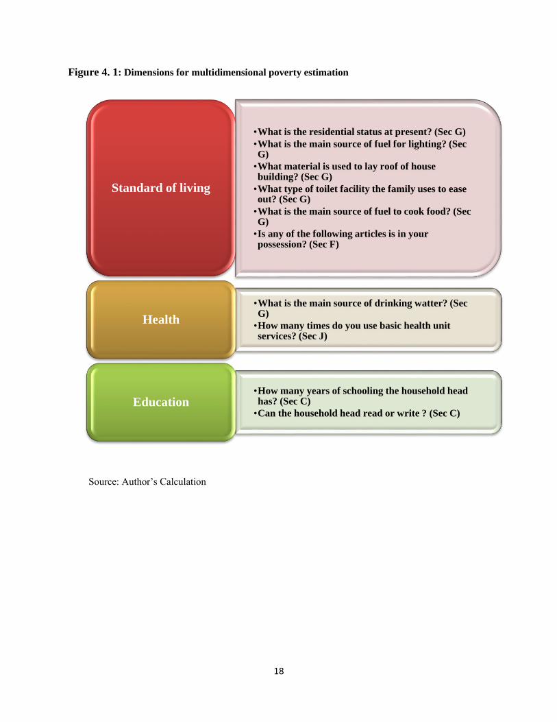
4.3 Multidimensional Poverty

The non-income indicators for measuring multidimensional poverty using alkire and foster

method take most of the variables from section G of PSLM 2010-11 at district level. However,

some of the non-income indicators are also taken from section J and section C & section F. The

relevant questions in their standard HIES forms taken up from different sections are shown in

figure 4.1. The 10 non-income indicators are bundled into three dimensions of standard of living,

health and education. There is dual cut off approach is used. The deprivation cut-off is based on

the MDGs and SDGs (Appendix C) In case of first indicator of standard of living those

households are deemed deprived if they are living on rent or subsidized rent. In STATA this

variable is recoded accordingly and new labels are subsequently attached to that variable to

designate whether the household has ownership or no ownership. Similarly, as for the second

indicator in living standard of source of fuel lighting is adjusted in STATA by labeling

electricity, gas, and kerosene oil as improved electricity sources while the remaining like candle,

fire-wood, and other sources are regarded as not improved. The roof indicator is recorded by

naming those households as having an improved roof type who have roof made up of RCC/RBC,

17

Iron/Cement sheets or other while not improved in case of wood/bamboo. The fourth indicator in

this dimension is recoded in STATA by considering those households deprived whose toilet

facility is not available, or uses a digged ditch, or a flush connected to open drain, or other

sources of easing out while those using flush system (linked to sewerage), flush system (linked to

septic tank), or privy seat are considered not deprived. The fifth indicator in this dimension of

source of fuel for cooking is recorded by considering households having an improved source of

cooking fuel who are using electricity, gas, or kerosene oil as a source of fuel of cooking while

other sources like cow-dung cakes, coal/wooden coal, fire-wood, sticks etc. or other sources are

labeled as not improved. Another non-income indicator taken from this section G is that of water

source which comes under the health dimension. It considers households as having safe water

drinking source if they use tap (in home), tap (outside home), hand pump, water motor, covered

well, tanker truck/water fetcher, or mineral water. Similarly, those using open well,

river/stream/pond etc. or any other sources coded as not using safe drinking water.

The last indicator in standard of living dimension related to assets assigns a value of 1 to

household if it possesses one of the following assets: 1) agriculture land; 2) car; 3 )television; 4)

refrigerator; 5) motorcycle; 5) AC; 6) washing machine or; 7) sewing machine. In order to

accomplish this Sec F of PSLM 2010-11 at district is used. As for the other indicator of health

dimension of frequency of visits to basic health units by household, Sec J is used. The relevant

question in PSLM2010-11(district level) has a total of four options; 1) not at all; 2) once a while;

3) often; and 4) always. This question is recorded by giving a value of 1 to household who visit

basic health units often or always while the remaining is assigned a 0 value. This adjustment is

further labeled according and those households who visit basic health units always or often are

deemed not deprived.

Finally the last dimension of education is based entirely on Section C where three

questions are considered. Firstly, the maximum education achieved is taken as number of the

years of schooling of the household head as the numeric values assigned in this question by

PSLM are consistent with the years of schooling. Household head with less than 6 years of

schooling are deemed as deprived in the present study. The other indicator of education

dimension is whether household head can read, write, and is able to conduct basic arithmetic

operations simultaneously is deemed as literate and illiterate otherwise. The resultant files are

merged together with hhcode as the identifier and afterwards Alkire and Foster method of

multidimensional poverty is used calculated summary index of multidimensional poverty i.e.

adjusted headcount ratio (M0). Appendix B.5 illustrates the do-file for the entire process.

Furthermore, the categories of understudy indicators for each dimension that are deemed poor

are shown in table 4.4 where categories that are considered deprived are bolded. Furthermore,

equal weights are assigned to each dimension in calculation of Alkire and Foster adjusted

headcount i.e. one-thirds. Similarly, each indicator within a dimension is given equal weight. The

weight for each indicator is calculated by multiplying the total number of indicators with the

weight of dimension in which that indicator is and sub-weight of each indicator within the

dimension as shown in table 4.5.

18

Figure 4. 1: Dimensions for multidimensional poverty estimation

Source: Author’s Calculation

•What is the residential status at present? (Sec G)

•What is the main source of fuel for lighting? (Sec G)

•What material is used to lay roof of house building? (Sec G)

•What type of toilet facility the family uses to ease out? (Sec G)

•What is the main source of fuel to cook food? (Sec G)

•Is any of the following articles is in your possession? (Sec F)

Standard of living

•What is the main source of drinking watter? (Sec G)

•How many times do you use basic health unit services? (Sec J)

Health

•How many years of schooling the household head has? (Sec C)

•Can the household head read or write ? (Sec C)Education

19

Table 4. 4: The cut-off point for each indicator of dimensions

Dimensions Question/Indicators Indicators’ cut-off

Standard of Living Residential Status (SDG 9) On rent, subsidized rent, personal residence (self-

hired), personal residence (hired), without rent

Energy Source for

electricity (SDG 7)

Candle, Fire-wood, other, electricity, gas , kerosene

oil.

Type of roof (SDG 11) Wood/Bamboo, other, RCC/RBC, Iron/Cement

Type of toilet facility

(SDG 11/7, MDG 7.9) Facility not available, digged ditch, flush

(connected to open drain, other, privy seat, flush

(linked to septic tank), flush (linked to sewerage)

Cooking fuel

(SDG 7, MDG 7) Fire-wood, sticks etc, cow-dung cakes,

coal/wooden coal, other, gas, kerosene oil,

electricity.

Assets

(SDG 1, MDG 1) Doesn’t possesses any of the following:

Tv, ac, refrigerator, sewing machine, washing

machine, motor cycle, agriculture land, does

posses these assets.

Health Water source

(SDG 11/3, MDG 7.8)

Open well,river/stream/pond etc, other, tanker

truck/water fetcher, water motor, covered well,

mineral water, tap (outside home), tap (in courtyard),

hand pump.

Basic Health units (SDG

3)

Visits: not at all, once in a while, always, often.

Education Read/Write

(SDG 4, MDG 2) Can’t read/write, can’t conduct arithmetic

operations, can read/write, can conduct arithmetic

operations

Years of schooling

(SDG 4, MDG 2)

Less than 6 years of schooling, greater then equal to

6

Source: Author’s Calculation

Table 4. 5: Weighting scheme for each dimension and indicator

Dimensions Question/Indicators Dimension

Weights

Indicators Weights

Standard of Living Residential Status 0.33

(0.33)*(1/6)*10 = 0.55

Energy Source for

electricity

(0.33)*(1/6)*10 = 0.55

Type of roof (0.33)*(1/6)*10 = 0.55

Type of toilet facility (0.33)*(1/6)*10 = 0.55

Cooking fuel (0.33)*(1/6)*10 = 0.55

Assets (0.33)*(1/6)*10 = 0.55

Health Water source 0.33 (0.33)*(1/2)*10 = 1.67

Basic Health units (0.33)*(1/2)*10 = 1.67

Education Read/Write 0.33 (0.33)*(1/2)*10 = 1.67

Years of schooling (0.33)*(1/2)*10 = 1.67

Total 1 10

Source: Author’s Calculation

20

4.4 Poverty Maps

The disaggregated poverty estimates can be best shown on a map in which the intensity of the

color conveys the relative severity of poverty. In present study, poverty maps are built using

Adept maps that can be used within STATA user-interface using amap command which loads

the adept map console in STATA. The whole process hinges on shapefiles and database files

which can be obtained through the internet and these files include x and y coordinates for the

regions that need to be mapped. In case of Pakistan xy coordinates are downloaded from

Geocommons at district level for each province and for the country as a whole. However, since

Adept map is option based once amap command is typed in STATA its do-file can’t be shown.

Nevertheless, it is noted that amap command is used on the file with variable on uni-dimensional

and multidimensional poverty against each district.

21

Chapter 5

Results and Discussions

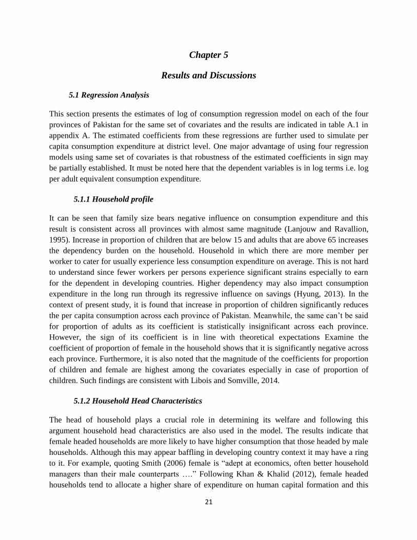
5.1 Regression Analysis

This section presents the estimates of log of consumption regression model on each of the four

provinces of Pakistan for the same set of covariates and the results are indicated in table A.1 in

appendix A. The estimated coefficients from these regressions are further used to simulate per

capita consumption expenditure at district level. One major advantage of using four regression

models using same set of covariates is that robustness of the estimated coefficients in sign may

be partially established. It must be noted here that the dependent variables is in log terms i.e. log

per adult equivalent consumption expenditure.

5.1.1 Household profile

It can be seen that family size bears negative influence on consumption expenditure and this

result is consistent across all provinces with almost same magnitude (Lanjouw and Ravallion,

1995). Increase in proportion of children that are below 15 and adults that are above 65 increases

the dependency burden on the household. Household in which there are more member per

worker to cater for usually experience less consumption expenditure on average. This is not hard

to understand since fewer workers per persons experience significant strains especially to earn

for the dependent in developing countries. Higher dependency may also impact consumption

expenditure in the long run through its regressive influence on savings (Hyung, 2013). In the

context of present study, it is found that increase in proportion of children significantly reduces

the per capita consumption across each province of Pakistan. Meanwhile, the same can’t be said

for proportion of adults as its coefficient is statistically insignificant across each province.

However, the sign of its coefficient is in line with theoretical expectations Examine the

coefficient of proportion of female in the household shows that it is significantly negative across

each province. Furthermore, it is also noted that the magnitude of the coefficients for proportion

of children and female are highest among the covariates especially in case of proportion of

children. Such findings are consistent with Libois and Somville, 2014.

5.1.2 Household Head Characteristics

The head of household plays a crucial role in determining its welfare and following this

argument household head characteristics are also used in the model. The results indicate that

female headed households are more likely to have higher consumption that those headed by male

households. Although this may appear baffling in developing country context it may have a ring

to it. For example, quoting Smith (2006) female is “adept at economics, often better household

managers than their male counterparts ….” Following Khan & Khalid (2012), female headed

households tend to allocate a higher share of expenditure on human capital formation and this

22

ultimately increases consumption also through enhanced employment chances. The correlate is

found to be significant in all provinces except Sindh. The age of the household head is estimated

to be positive and significant in case of Punjab, Sindh, and Balochistan. The positive relationship

in case of Punjab and Sindh might be explained in terms of the role that experience plays in

enhancing the employability of an individual which help secure a stable consumption pattern.

Recognizing the importance of age of household head as a major determinant of consumption

expenditure, Radivojevic & Vasic (2012) have referred to the family life-cycle hypothesis. The

result for the age variable is also supported by Caglayan and Astar (2012). Contrarily, the

negative relationship between consumption and age of household head found in case of

Balochistan may be explained by the fact that household head having crossed a certain threshold

of age may find their employability diminished as employers prefer younger and more energetic

workers to old.

The types of employment of household head and consumption expenditure tend to have an

intricate relationship. While most types bear a positive sign except few types in some provinces;

most of them are consistently insignificant across each province. However, most of them are

significant in no more than two provinces like employer greater than 10, owner cultivator, share

cropper, contract cultivator, and livestock. Moreover, it is observed that employer of less than 10

is significant in three provinces i.e. Sind, KPK, and Balochistan. Furthermore, the significance

of different categories in different provinces might hint towards the relative importance of that

particular employment type for increasing consumption in the respective province. For example,

owner cultivator and share cropper can increase consumption expenditure in Sindh and

Balochistan while the same can be said for contract cultivator in case of Punjab. Another vivid

observation is that most of employment sources are significant and relevant in case of

Balochistan and an unpaid family worker bears no significant impact on consumption. The last

variable of household head characteristics is education of head. The estimated coefficients are

positive in case of primary education they still is insignificant implying no empirical relevance.

However, any further increases in education can increase consumption expenditure

proportionally. In case of this research, the estimated coefficients tend to be higher for degree

education dummy than for secondary and primary education dummy. This suggests that any form

of education greater than primary can be pivotal for increasing consumption expenditure. There

exists a bulk of literature that addresses the importance of education in increasing welfare (Roos

et al., 2001; Caglayan, E., & Astar, M.,2012); Gounder, 2012; Talukder & Chile, 2013).

23

5.1.3 Household Welfare Characteristics

Moving towards the household welfare characteristics, only number of rooms is found to be

significantly exerting positive influence on consumption expenditure with slight variation in

magnitude of estimated coefficient across provinces. Similarly, roof type is significant in three

provinces except Balochistan while cooking source is significant and positive in Punjab only.

The relationship between most of the non-income indicators and consumption expenditure seem

perplexing. However, one way to explain such insignificant relationship in case of most

variables can be that consumption expenditure calculation in Pakistan does not take into account

expenses incurred on durables. It may be possible that household that purchase their personal

home or start using an expensive albeit safe drinking water source as well as improved toilet

facility may have to compromise their consumption of non-durable goods which are used in

consumption calculation. In this case, such expenditure may become substitute of each another.

Yang (2005) suggests that household do compromise non-housing expenditure to build stock of

housing. This can be the basis of the argument mentioned above in explaining insignificant

relationship between some of the household welfare characteristics and consumption

expenditure. However, a stronger explanation for this can be in terms of correlation. Since,

estimated beta coefficients can also be interpreted as a shadow measure of correlation between

the consumption expenditure and the concerned variable it won’t be wrong to state that contrarily

to often quoted believe that non-income indicators are correlated to income gains they are

actually not as no statistical linkage between the two can be established.

5.1.4 Assets

Finally, assets seem to have a strong overall relationship with consumption expenditure. In order

to shed light on these results, one must understand that assets like a/c, refrigerator, car, and

motorcycle to some extent don’t fall in low-income category. For example, only those

households can afford such articles that already enjoy a high level of consumption. However, in

case of agriculture and livestock ownership it is safer to use the value-addition argument of such

assets since they can be a catalyst of high consumption. As opposed to the relationship between

non-income indicators of household welfare and consumption expenditure the relationship

between consumption expenditure and assets seem consistent. This may imply that income

poverty go hand in hand with asset poverty. Resultantly, the sensitivity of assets to gains in

income is more than that of non-income welfare indicators. In order to use the estimated

coefficients for simulating consumption expenditure per head it is a must to have a model that

exhibits an improved fit. This is assessed by the fact that adjusted R-square is reasonably high

for each province. Some of the variables are also deliberately added in a way that improves the

fit.

24

5.2 Uni-dimensional poverty across sub-regions of Provinces

The poverty estimates at the provincial level in figure are based on HIES survey data since it is

representative at provincial level. Further disaggregation of poverty at division and district level

is carried out by using small area estimation which is addressed in the later section of this

chapter. One of the over-riding conclusions in poverty analysis of Pakistan is the fact that

poverty has been and still remains a rural phenomenon in the country (UDNP, 2011; Arif &

Farooq, 2011; and Cheema & Sial, 2014.) This pattern is also consistent when one compares the

urban and rural incidence of poverty across each province of Pakistan as seen in figure 5.1.

However, the extent of the diversion in rural and urban poverty varies across each province. The

difference between rural and urban poverty in case of Punjab is highest followed by that in

Balochistan, Sindh and KPK. However, the incidence of rural poverty is highest in Punjab and

least in KPK. As for urban poverty, Sindh posts the lowest rate mainly because it includes the

financial hub of the country i.e. Karachi which is the most representative district among Sindh

province’s sampled households. The lower-than-expected figures of poverty in Balochistan and

KPK may be due to the fact that these regions are conflict prone which hinders the data

collection efforts and also impacts the quality of the data. Resultantly, easy-to-access and

relatively rich areas are covered in the data collection. This assertion is also recognized in the

latest report by Federal Bureau of Statistics (FBS, 2015). It is also observed that rural poverty in

Punjab is highest than Sindh, KPK, and Balochistan. This is due the fact that Punjab is home to

two out of four deserts of Pakistan and its southern region is notoriously poor. This assertion can

be supplemented by the findings of Cheema and Sial (2014) using HIES, 2010-11.

Figure 5. 1: Poverty estimates - Uni-Dimensional

7.6

15.0

7.1 7.4 6.9

18.3

4.3

9.8

05

10

15

20

Headcount

Ratio

Balochistan KPK Punjab Sindh

Source: Author's Calculation Using Smalll Area Estimation

Unidimensional

Rural/Urban Poverty in Provinces of Pakistan

Urban Rural

25

5.3 Multidimensional poverty across sub-regions of Provinces

The section presents the estimates of multidimensional poverty using Alkire and Foster adjusted

headcount ratio. The figure 5.2 shows that rural and urban sector of Balochistan is most poor

followed by KPK, Sindh, and Punjab. Comparing these results with uni-dimensional poverty

measures in figure 5.1 shows that apart from urban sector of Punjab, adjusted headcount ratio is

higher across each provinces and across each sector. This lays down that uni-dimensional

approach to poverty assessment underestimates the relative extent of deprivation in well-being.

Further comparison makes the polarizing results clearer. For instance, Punjab’s rural sector was

most poor using consumption as well-being measure. However, when non-income indicators are

used the situation is reversed completely with Punjab’s rural sector being the least poor relative

to other provinces’ rural sector. Similarly, Sindh’s urban sector also undergoes positional change

as it now becomes the second least poor urban sector of the country with reference to other

provinces’ urban sector. However, some of the patterns are similar. Sindh’s rural sector is still

less poor than KPK’s rural sector while Balochistan’s urban sector is also poorer than KPK’s,

Punjab’s, and Sindh’s urban sector.

Figure 5. 1: Multidimensional Poverty

5.4 District/Division level Poverty Rates using simulated consumption

This section presents the district and division level poverty estimates using both uni-dimensional

and multi-dimensional approach to poverty. It is mentioned here that division is an

administrative region in Pakistan which comprises of few districts. Furthermore, results are

mapped to shed light on the spatial distribution of poverty estimates – both uni-dimensional and

multi-dimensional.

17.7

49.6

16.4

28.7

6.9

18.3

14.3

34.9

010

20

30

40

50

Headcount

Ratio

Balochistan KPK Punjab Sindh

Source: Author's Calculation using PSLM, 2010-11

Multidimensional

Poverty Estimates at Provincial Level in Pakistan

Urban Rural

26

5.4.1 Punjab

In case of Punjab, districts in the northern part of the province like Rawalpindi, Chakwal, and

Jhelum are least poor while Rajan Pur is the poorest district followed by Muzaffar Garh, D. G.

Khan, and Rahim Yar Khan as shown in table 5.1. Similarly, the big cities of the province which

are spread unevenly across the province record minimum poverty incidence uni-dimensionally

(multidimensionally) like Lahore which records a poverty rate of 9.65 (14) percent, Sialkot 10.24

(19.1), Gujranawala12.78 (19.6), Sargodha 15.35(24.2) percent. By comparing multi-

dimensional poverty incidence with uni-dimensional poverty incidence, the adjusted headcount

ratio record higher figures consistently for each district except Rajan Pur, Muzaffargarh, D.G.

Khan, Layyah, and Jhang. Among the ten poorest districts of the province uni-dimensionally

seven are situated in the southern part of the province while the remaining three belong to central

region. The same pattern is also observed in case of multidimensional poverty as six districts are

located in south Punjab among ten most poor districts. Similarly, eight and seven districts belong

to north Punjab among least poor districts uni-dimensionally and multi-dimensionally

respectively. This suggests the South Punjab is poorer than central and north Punjab. Hence, a

spatially skewed incidence of poverty in the province is quite evident as shown in figures A.2 in

Appendix A., Interestingly; a cursory look on the map can reveal that districts constituting the

Thall Desert region in Punjab like Bhakkar, Layyah, Muzaffargarh, and Jhang are marked by

high or high extreme poverty both uni-dimensionally and multi-dimensionally. Similarly,

districts constituting Cholistan Desert like Bahawalnagar and Bahawalpur are also among the

poorest.

5.4.2 Sindh

Sindh’s state of disaggregated poverty shows a pattern closer to that of Punjab in terms of

geographical spatial setting of poverty pockets. It is no wonder that Karachi is the least poor

district of the province; in fact it is one the least poor district of the entire country excluding the

capital territory. In terms of uni-dimensionl poverty rate Jacobabad, Larkana, Tharparkar and

Kashmore are the most poor districts of the province with poverty rate of 22.97 percent, 22.66

percent, 22.65 percent, and 21.71 percent respectively as shown in table 5.2. However, a

comparison with multidimensional adjusted headcount ratio reveals that all districts and

divisions of the province register high incidence of multidimensional poverty. This is opposite to

what is viewed in Punjab where five districts were found to be less multidimensionally poor and

more uni-dimensionally poor. This can hint towards the fact that Sindh’s achievement in non-

income indicators may have been rather dismal relative to that of Punjab. Another observation

from table 5.2 is that with reference to Punjab the adjusted headcount ratios are higher on

average than that for the districts and divisions of Punjab. Sindh’s ten most poor districts are

evenly balanced among south and north regions with six and four in north and south respectively

when uni-dimensional poverty estimates are assessed. This may result from the fact that districts

in north Sindh are attached with South Punjab which as mentioned above is a hotbed of poverty

27

in Punjab province. The situation is reserved in case of multi-dimensional poverty estimates

which record six districts of south Sindh among ten more poor districts. Nevertheless, the five

poorest districts are all located in the southern part of the province when adjusted headcount is

observed. This is self-evident since districts in the south of Sindh like Thatta and Tharparkar are

notorious for incidence of droughts and famines. It is noted that Tharparkar is currently famine-

stricken at the time of writing. This is not hard to understand since these districts form part of

Thar Desert which is the 17th largest desert in the world. In fact, it won’t be wrong to say that

districts forming the whole of Thar Desert are among poorest. Therefore, it can be concluded that

Northern and Southern tip of the province are marked by high rate of deprivation uni-

dimensionally while the incidence of multi-dimensional poverty is higher in case of latter as

illustrated in figures A.3 in Appendix A.

5.4.3 KPK

KPK as a province can lend valuable lessons in the context of geography of poverty since it is a

combination of agrarian lands, mountains, and steppes in some cases. In terms of uni-

dimensional poverty, table 5.3 shows that Bonair has highest incidence of poverty in the

province with a poverty rate of 23.79 percent. Karak clocks in at 23.11 percent as the second

poorest district followed by Lakki Marwat at 20.97 percent. Surprisingly, KPK has the second

least poor district of the country i.e. Abottabad with a predicted headcount ratio of 6.97 percent.

Districts closer to Islamabad and Rawalpindi Division are least poor districts of the province like

Haripur and Abbottabad as a result of positive spatial externality. Hence, a clear difference

between these two districts and the other districts of the province is clearly visible. Subsequently,

among ten most poor districts four belong to south KPK while three each belong to north and

central KPK. The districts with mountains like those in Malakand division are among most poor

when adjusted headcount is observed and so are the southern districts in Kohat and Bannu

divisions as they mostly constitute dry mountains region. The southern D. I. Khan and Kohat

divisions are poorer with adjusted headcount ratio of 37.5 percent and 35 percent respectively.

As in Sindh, all of the districts in KPK are poorer when attention is changed to multidimensional

poverty from its uni-dimension counterpart. It is noted that among the ten poorest districts of the

province multidimensinoally, five are in the northern mountain region while one is in the

southern mountain region. As a result, it can be safely said that poverty incidence among

mountain regions be it snow-capped in the north or parched-tipped in the south is high.

Subsequently, a geographically spaced distribution of poverty is quite vivid as shown in figures

A.4.

5.4.4 Balochistan

Balochistan’s northwestern districts post low poverty level uni-dimensionally as table 5.4 reads.

Some of the least poor districts of Balochistan are Ziarat, Sibbi, Harnai, Kahlu, Quetta, Pashin,

Qilla Abdullah and Mashtung. Apart from Awaran all of these districts are situated just below

28

the northern part of the province as presented in figures A.4 in appendix A.. These surprisingly

low estimates of unidimensional poverty do not seem sound as it is believed that Balochistan is

the most destitute province of the country. Explanation for this can be direct to the fact that

quality of data for Balochistan is of rather dubious research and this is not the first time that such

low estimates are obtained for Balochistan (Anwar & Qureshi, 2002; Saboor, 2004; Malik, 2005;

Arif, 2006) However, when attention is directed to multi-dimensional poverty estimates a rather

gloomy picture is painted. The concept of first-city bias is so much evident in case of

Balochistan that apart from its capital i.e. Quetta and its adjacent district Pashin all of the

districts have adjusted headcount ratio of no less than 30 percent. This augur that Balochistan

will remain under-privileged part of the country unless and until non-income indicators are

addressed since monetary yardstick understates the poverty incidence by a wide margin. Even in

case of Quetta and Pashin the poverty rates jumps from 4.18 to 17.4 and 3.48 to 18.9 percent

respectively when uni-dimensional approach to poverty is substituted with multidimensional

poverty. It can be observed that districts adjoining south Punjab and north Sindh like Dera Bugti,

Loralai, Kohlu, and Barkhan show extreme poverty in terms of uni-dimensional and multi-

dimensional. Furthermore, it also observed district of Chagai which encompasses the Kharan

Deseart is extremely poor both uni-dimensionally and multi-dimensionally as shown in figures

A.5 in appendix A.

5.4.5 Pakistan

Provincial distribution of poverty incidence is skewed and the same pattern is also valid for the

country as well. In nutshell, while south Punjab districts clustered together are the poorest

regions of the country unidimensionally the picture turns drastically reverse when

multidimensional poverty map is viewed in figure A.5 in appendix A.. In multidimensional

poverty assessment the poorest regions are now situated in Balochistan, Southern KPK and

Southern Sindh. A close look of the map reveals that not a single district of Punjab appears

among the poorest district of Pakistan multidimensionally. However, middle-high poverty is still

retained in the districts covering the Thall and Kohistan Deserts.

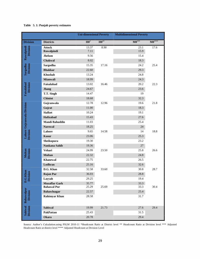
29

Table 5. 1: Punjab poverty estimates

Source: Author’s Calculation.using PSLM 2010-11 *Headcount Ratio at District level ** Headcount Ratio at Division level *** Adjusted

Headcount Ratio at district level **** Adjusted Headcount at Division Level

Uni-dimensional Poverty Multidimensional Poverty

Division Districts H0* H0** M0*** M0****

Ra

wa

lpin

di

Div

isio

n

Attock 13.37 8.90 23.1 17.6

Rawalpindi 7.11 15.9

Jhelum 9.56 15.4

Chakwal 8.02 18.3

Sa

rgod

ha

Div

isio

n

Sargodha 15.35 17.16 24.2 25.4

Bhakkar 22.60 29.3

Khushab 13.24 24.8

Mianwali 18.99 24.3

Fa

isa

lab

ad

Div

isio

n

Faisalabad 13.02 16.46 20.2 22.3

Jhang 24.67 23.6

T.T. Singh 14.47 19

Chiniot 18.68 32.3

Gu

jra

nw

ala

Div

isio

n

Gujranwala 12.78 12.96 19.6 21.8

Gujrat 11.00 18.3

Sialkot 10.24 19.1

Hafizabad 15.43 27.6

Mandi Bahuddin 11.03 25.4

Narowal 18.25 24

La

ho

re

Div

isio

n

Lahore 9.65 14.58 14 18.8

Kasur 23.06 25.3

Sheikupura 19.30 23.2

Nankana Sahib 19.36 27

Mu

lta

n

Div

isio

n

Vehari 24.99 23.50 25.8 26.6

Multan 22.32 24.8

Khanewal 22.75 26.5

Lodhran 25.16 32.6

D.G

.Kh

an

Div

isio

n D.G. Khan 32.58 33.60 30.8 28.7

Rajan Pur 36.03 28.8

Layyah 29.25 19.4

Muzaffar Garh 35.77 33.3

Ba

ha

wa

lpu

r

Div

isio

n

Bahawal Pur 25.29 25.69 33.3 30.4

Bahawlnagar 22.57 25.4

Rahimyar Khan 28.58 31.7

Sa

hiw

al

Div

isio

n

Sahiwal 19.99 21.73 27.6 29.4

PakPattan 25.43 31.5

Okara 20.78 29.4

30

Table 5. 2: Sindh poverty estimates

Source: Author’s Calculation.using PSLM 2010-11 *Headcount Ratio at District level ** Headcount Ratio at Division level *** Adjusted

Headcount Ratio at district level **** Adjusted Headcount at Division Level

Uni-Dimensional Poverty Multidimensional Poverty

Divisions Districts H0* H0** M0*** M0****

SU

KK

UR

DIV

ISIO

N Khairpur 14.46 15.84 27.7 25.9

Sukkur 16.00 24.2

Nawabshah 13.85 31.2

Nowsheroferoz 17.06 20.1

Ghotki 17.85 26.8

LA

RK

AN

A

DIV

ISIO

N Jacobabad 22.97 21.58 34.6 28.2

Kashmore 21.71 30.9

Shikarpur 19.65 28

Larkana 22.66 23.4

ShahdatKot 21.36 25.4

HY

DE

RA

BA

D

DIV

ISIO

N

Dadu 12.46 15.19 24.2 32

Jamshoro 16.85 31.2

Hyderabad 9.22 19.9

Matiari 14.30 30.4

Tandoallahyar 12.86 30

Tandomuhdkhan 17.63 37.4

Badin 18.40 37.9

Thatta 19.04 42.5

MIR

PU

RK

HA

N

DIV

ISIO

N

Sanghar 14.45 17.72 22.9 34.6

MirphurKhas 16.02 33.1

Umerkot 19.05 42.2

Tharparkar 22.65 44.4

KA

RA

CH

I

DIV

ISIO

N Karachi 4.35 4.35 12.3 12.3

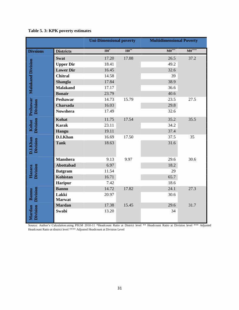
31

Table 5. 3: KPK poverty estimates

Uni-Dimensional poverty Multidimensional Poverty

Divsions Districts H0* H0** M0*** M0****

Ma

lak

an

d D

ivis

ion

Swat 17.20 17.88 26.5 37.2

Upper Dir 18.41 49.2

Lower Dir 16.45 32.6

Chitral 14.58 39

Shangla 17.84 38.9

Malakand 17.17 36.6

Bonair 23.79 40.6

Pes

ha

wa

r

Div

isio

n Peshawar 14.73 15.79 23.5 27.5

Charsada 16.03 29.8

Nowshera 17.49 32.6

Koh

at

Div

isio

n

Kohat 11.75 17.54 35.2 35.5

Karak 23.11 34.2

Hangu 19.11 37.4

D.I

.Kh

an

Div

isio

n D.I.Khan 16.69 17.50 37.5 35

Tank 18.63 31.6

Haza

ra

Div

isio

n

Manshera 9.13 9.97 29.6 30.6

Abottabad 6.97 18.2

Batgram 11.54 29

Kohistan 16.71 65.7

Haripur 7.42 18.6

Ban

nu

Div

isio

n

Bannu 14.72 17.82 24.1 27.3

Lakki

Marwat

20.97 30.6

Ma

rdan

Div

isio

n Mardan 17.38 15.45 29.6 31.7

Swabi 13.20 34

Source: Author’s Calculation.using PSLM 2010-11 *Headcount Ratio at District level ** Headcount Ratio at Division level *** Adjusted

Headcount Ratio at district level **** Adjusted Headcount at Division Level

32

Table 5. 4: Balochistan poverty estimates

Divsions Districts Unidimensional Multidimensional

H0* H0** M0*** M0****

Qu

etta

Div

isio

n

Quetta 4.18 9.06 17.4 33.9

Pashin 3.48 18.9

Qilla Abdullah 3.89 37.9

Chagi 19.26 56.8

Sib

bi

Div

isio

n Nushki 17.84 7.71

52.3 43.2

Sibbi 3.59 26.2

Ziarat 3.91 30.1

Kohlu 6.62 57.6

Derag Bugti 19.42 65.7

Kala

t D

ivis

ion

Harnai 5.19 11.24 38.6 43.6

Kalat 9.38 39

Mastung 7.52 30.9

Khuzdar 11.70 36.8

Awaran 7.93 40.3

Kharan 15.09 53.5

Washuk 11.35 52

Lasbilla 13.91 48.8

Mek

ran

Div

isio

n Ketch/Turbat 13.50 12.37 44.5 43.9

Gwadar 10.88 37.1

Panjgur 12.51 50.6

Zh

ob

Div

isio

n Zhob 12.35 15.47 43.4 51.2

Lorali 19.77 52.6

Barkhan 14.38 60.3

Muskhel 29.13 53.5

Qillah Saifullah 9.58 50.9

Sherani 8.39 48.2

Na

sira

ba

d

Div

isio

n

Nasirabad 20.88 16.72 49.4 46.6

Jafarabad 18.81 41

Jhal Magsi 13.21 53.9

Bolan/Kacchi 13.35 43.2

Source: Author’s Calculation.using PSLM 2010-11 *Headcount Ratio at District level ** Headcount Ratio at Division level *** Adjusted

Headcount Ratio at district level **** Adjusted Headcount at Division Level

33

5.5 Reliability of the maps

To ascertain whether the estimates obtained using SAE are reliable; z-score is calculated for

selected set of divisions in each province. These divisions are selected on the basis of coverage

of households in the survey. While the application of this test may have been more informative

if carried out for each district; it is reiterated here that HIES is not representative at district level.

Based on this, divisions are selected since each division comprises of some districts and

resultantly, a reasonable amount of households can be covered in it. Three divisions are selected

from Punjab while only two divisions each are picked from remaining three provinces.

Subsequently, the z-score value should not exceed 2 if both poverty estimates are to represent the

same poverty incidence. The results in table 4.5 show that values of z-score are well within the

accepted bounds for each division; thus establishing the reliability of the maps. The Survey Data

Estimates in the table 5.5 below are based on HIES dataset while Predicted SAE Estimates are

taken from tables 5.1 to 5.4 against the relevant division.

Table 5. 5: Reliability Test

Source: Author’s Calculation

Table 4.4: Reliability Test

Note: z-score = (H0(SAE) – H0(Survey))/[(SE(SAE))2+ (SE(Survey))

2]

0.5

Divisions Survey Data Estimates Predicted SAE Estimates Z-score

No. of

households

H0 No. of

households

H0

Lahore Mean 848 0.146 4900 0.145 -0.042

Std. Error 0.012 0.003

Multan Mean 575 0.249 3561 0.235 -0.729

Std. Error 0.018 0.004

Bahawalpur Mean 591 0.245 3212 0.257 0.624 Std. Error 0.018 0.005

Karachi Mean 822 0.057 4414 0.043 -1.678

Std. Error 0.008 0.002

Hyderabad Mean 873 0.166 5203 0.152 -0.748

Std. Error 0.013 0.003

Malakand Mean 511 0.200 3424 0.178 -1.190 Std. Error 0.018 0.003

Pewhawar Mean 487 0.175 2211 0.157 -0.971

Std. Error 0.017 0.004

Quetta Mean 488 0.117 2332 0.091 -1.745 Std. Error 0.015 0.003

Nasirabad Mean 287 0.157 1571 0.167 0.500

Std. Error 0.021 0.005

34

Chapter 6

Conclusion

In an attempt to map unidimensional poverty in Pakistan at disaggregated level in Pakistan; small

area estimation technique is used using HIES and PSLM data for the same year i.e. 2010-11.

Furthermore, unidimensional poverty maps are supplemented with multidimensional poverty

maps. It is observed that unidimensional poverty estimates consistently underestimate poverty

when its results are compared against multidimensional poverty. However, exceptions to this

pattern are few. This emphasizes that poverty exuberates when social sector performance in the

districts of the country is evaluated which permits the conclusion that Pakistan’s achievement in

social sectors is dismal. Similarly, monetary poverty in Pakistan is observed to be more clustered

in the Southern region of Punjab and the districts of other provinces adjacent to South Punjab.

This indicates that poverty in Pakistan has the characteristics of spilling over to other regions

adjoining it which implies existence of negative spatial externality. This reiterates that geography

as a determinant of poverty has serious implication on poverty. However, the same can’t be said

for multidimensional poverty as its incidence is more specific to the geography of the regions

like deserts and mountains. Poverty is also observed to have a location characteristic in Pakistan

especially in Punjab. Districts located in the south of Punjab, North/south of Sindh, South of

KPK, and west/east of Balochistan are poorer in nature. Therefore, it can be concluded that as

poverty is not equally spread among countries; the same is also true within country.

6.1 Recommendations

Based on these observations, it can be concluded that a spatial distribution of poverty is evident

in Pakistan and subsequently necessitates the need to incorporate concerns for geographical

targeting of poverty. On the same lines, it is emphasized that regional-specific policies give more

consideration towards conflict-ridden provinces of Balochistan and KPK to tackle the lagging

social sectors in these provinces. This can be accomplished by delegating administrative powers

to districts and removing any political bottlenecks that hinders it because problems can be best

sorted out by the population indigenous to it. Furthermore, it is suggested that PSLM data to be

complied every time HIES survey is conducted so that poverty mapping using methods like

small area estimation is carried out frequently. Finally, as opposed to district level poverty

mapping conducted in the present study; country-wide poverty mapping at tehsil level which

forms the lowest tier in the administrative hierarchy of the Pakistan can also be informative. In

this way, updated information on disaggregated poverty will be available to policy makers which

can help them to not only gauge performance of their policies but also identify regions that are

lagging behind persistently.

35

Bibliography

Alkire, S, and Santos, M. E. (2010), Acute multidimensional poverty: A new index for developing

countries. United Nations development programme human development report office background

paper 2010/11.

Amarasinghe, U., Samad, M., & Anputhas, M. (2005). Spatial clustering of rural poverty and food

insecurity in Sri Lanka. Food Policy, 30(5), 493-509.annali di economia", n.7-9, pp. 333-348.

Anwar, T., & Qureshi, S. K. (2002). Trends in absolute poverty in Pakistan: 1990-91 and 2001. The

Pakistan Development Review, 859-878.

Arif, G. M. 2006. The Reliability and Credibility of Statistical Data for Poverty Analysis in Pakistan.

Asian Development Bank.

Arif, G. M., & Farooq, S. (2011). Poverty, Inequality and Unemployment in Pakistan. Backgroung study

for IDB group MCPS Document for Pakistan. Dhul-Qa’dah H, 1432.

Arif, N., & Nazim, A. (2012). Clustered deprivation: district profile of poverty in Pakistan. Sustainable

Development Policy Institute (SDPI).

Baker, J. L., & Grosh, M. E. (1994). Poverty reduction through geographic targeting: How well does it

work?. World Development, 22(7), 983-995.

Bellon, M. R., Hodson, D., Bergvinson, D., Beck, D., Martinez-Romero, E., & Montoya, Y. (2005).

Targeting agricultural research to benefit poor farmers: Relating poverty mapping to maize

environments in Mexico. Food Policy, 30(5), 476-492.

Bigman, D., Dercon, S., Guillaume, D., & Lambotte, M. (2000). Community targeting for poverty

reduction in Burkina Faso. The World Bank Economic Review, 14(1), 167-193

Bourguignon, F., & Chakravarty, S. R. (2002). Multi-dimensional poverty orderings. Delta.

Bourguignon, F., & Chakravarty, S. R. (2003). The measurement of multidimensional poverty. The

Journal of Economic Inequality, 1(1), 25-49.

Burki, A. A., Memon, R., & Mir, K. (2015). Multiple Inequalities And Policies To Mitigate Inequality

Traps In Pakistan. OXFAM Research Report.

Caglayan, E., & Astar, M. (2012). A Microeconometric Analysis of Household Consumption Expenditure

Determinants for both Rural and Urban Areas in Turkey. American International Journal of

Contemporary Research, 2(2), 27-30.

36

Chakravarty, Satya R., and Jacques Silber. "Measuring multidimensional poverty: the axiomatic

approach." Quantitative approaches to multidimensional poverty measurement (2008): 192-209.

Chaudhry, I. S., & Rahman, S. (2009). The impact of gender inequality in education on rural poverty in

Pakistan: an empirical analysis. European Journal of Economics, Finance and Administrative

Sciences, 15, 174-188.

Cheema, A. R., & Sial, M. H. (2014). Poverty and Its Determinants in Pakistan: Evidence from Pslm

2010-11. Journal of Poverty, Investment and Development, 5, 1-16.

Cheema, A., Khalid, L., & Patnam, M. (2008). The geography of poverty: Evidence from the Punjab. The

Lahore Journal of Economics, 13, 163-188.

Clark, D. A. (2005). The Capability Approach: Its Development, Critiques and Recent Advances.

Accessed from http://economics.ouls.ox.ac.uk/14051/1/gprg-wps-032.pdf

Costa, M., & De Angelis, L. (2008). The multidimensional measurement of poverty: a fuzzy set approach.

Statistica, 68(3), 303-319.

Cuong, N. V., Truong, T. N., & Van Der Weide, R. (2010). Poverty and inequality maps in rural

Vietnam: An application of small area estimation. Asian Economic Journal, 24(4), 355-390.

Davis, B. (2003). Choosing a method for poverty mapping. Food & Agriculture Org.

Duclos, J. Y., Sahn, D. E., & Younger, S. D. (2006). Robust multidimensional poverty comparisons*. The

economic journal, 116(514), 943-968.

Elbers, C., Lanjouw, J. O., & Lanjouw, P. (2003). Micro–level estimation of poverty and

inequality. Econometrica, 71(1), 355-364.

Farrow, A., Larrea, C., Hyman, G., & Lema, G. (2005). Exploring the spatial variation of food poverty in

Ecuador. Food Policy, 30(5), 510-531.

Fidrmuc, J., & Senaj, M. (2012). Human Capital, Consumption, and Housing Wealth in Transition (Vol.

1) John Wiley and Sons Inc.

Filmer, D. 2000. The Structure of Social Disparities in Education: World Bank Policy Research Working

Paper 2268, Development Economics Research Group, World Bank, Washington, DC

Filmer, D., & Pritchett, L. H. (2001). Estimating wealth effects without expenditure Data—Or tears: An

application to educational enrollments in states of india*. Demography, 38(1), 115-132.

Findeis, J., Snyder, A., & Jayaraman, A. (2005). The well-being of US farm workers: employee benefits,

public assistance, and long-term effects. Applied Economic Perspectives and Policy, 27(3), 361-

368.

37

Ghosh, M., & Rao, J. N. K. (1994). Small area estimation: an appraisal. Statistical Science, 55-76.

Gounder, N. (2012). The determinants of household consumption and poverty in Fiji (No. economics:

201205).

Haslett, S., & Jones, G. (2008). Potential for Small Area Estimation and Poverty Mapping in Timor-

Leste.

Haughton, J and Khandker, S. H. (2009). Handbook on poverty and inequality. World Bank.,

Washington, D.C.

Hyman, G., Larrea, C., & Farrow, A. (2005). Methods, results and policy implications of poverty and

food security mapping assessments. Food Policy, 30(5), 453-460.

Hyung, J. 2013. An Analysis on the Effect of Old-age Dependency Ratio on Saving Rate. University of

California, Berkeley.

IMF. (2013). Pakistan: Poverty Reduction Strategy Paper.

Retrieved from http://www.imf.org/external/pubs/ft/scr/2010/cr10183.pdf

Jamal, H. (2007). Income poverty at district level: An application of small area estimation technique.

Social Policy and Development Centre.

Jamal, H. (2012). An Exploratory Analysis of Inter-Temporal Multidimensional Poverty (No. 83). SPDC

Research Report.

Jamal, H.(2009). Estimation of multidimensional poverty in Pakistan. Social Policy and Development

Centre.

Jiang, J., & Lahiri, P. (2006). Mixed model prediction and small area estimation. Test, 15(1), 1-96.

Kam, S. P., Hossain, M., Bose, M. L., & Villano, L. S. (2005). Spatial patterns of rural poverty and their

relationship with welfare-influencing factors in Bangladesh. Food Policy, 30(5), 551-567.

Khan, A. H., & Khalid, U. (2012). Consumption patterns of male and female headed households in

Pakistan: evidence from PSLM 2007-08. The Pakistan Development Review, 51(4-II), pp-465.

Kudebayeva, A. and A. Barrientos. 2013. A decade of poverty reduction in Kazakhstan 2000-2009:

growth and/or redistribution?,BWPI, The University of ManchesterJazib, Today 2:24 PM

Lanjouw, P., & Ravallion, M. (1995). Poverty and household size. The economic journal, 1415-

1434.Jazib, Today 4:17 PMYOU give 1995 but in write 994.

38

Libois, F., & Somville, V. (2014). Fertility, Household’s size and Poverty in Nepal. CMI Working Paper.

Malik, S. (2005). Agricultural growth and rural poverty: a review of evidence. Pakistan Resident

Mission Working Paper No. 2. Islamabad: Asian Development Bank.

Marker, D. A. (1999). Organization of Small Area Estimators Using a Generalized Linear

Regression Framework. Journal of Official Statistics, 15(1), 1.

Minot, N. (2000). Generating disaggregated poverty maps: An application to Vietnam. World

Development, 28(2), 319-331.

Mishra, S., & Pathak, D. C. (2011). Poverty Estimates in India: Old and New Methods, 2004-05.

Moav, O., & Neeman, Z. (2008). Conspicuous consumption, human capital, and poverty. Human Capital,

and Poverty (June 9, 2008).

Noble, A. (2003). Small area estimation through glm. Unpublished Thesis, Massey University, New

Zealand.

Federal Bureau of Statistics. 2014

Parker, J. A. (1999). The consumption function re-estimated. Princeton University.

Petras, J., & Veltmeyer, H. (2007). The ‘development state’in Latin America: whose development, whose

state?. The Journal of Peasant Studies, 34(3-4), 371-407.

Radivojević, B., & Vasić, P. (2012). Household age structure and consumption in Serbia. Economic

annals, 57(195), 79-101.

Rao, J. N. (2003). Small area estimation. John Wiley & Sons, Inc..

Ravallion, Martin. "Measuring social welfare with and without poverty lines."The American economic

review (1994): 359-364.

Roelen, K., Gassmann, F., & de Neubourg, C. (2010). Child poverty in Vietnam: Providing insights using

a country-specific and multidimensional model. Social indicators research, 98(1), 129-145.

Roos G, Johansson L, Kasmel A, Klumbiene J & Prättälä R (2001): Disparities in vegetable and fruit

consumption: European cases from the North to the South. Public Health Nutr. 4, 35–43

Saboor, A. (2004). Agricultural growth, rural poverty and income inequality in Pakistan: A Time series

analysis. Department of Agricultural Economics, University of agriculture, Faisalabad, Pakistan

Said, F., Musaddiq, T., & Mahmud, M. (2011). Macro level Determinants of Poverty: Investigation

through poverty mapping of districts of Pakistan. The Pakistan Development Review, 895-910.

39

Sen A.K. (1985). Commodities and capabilities, Amsterdam, North Holland.

Sen A.K. (1987). The standard of living, Cambridge University Press, Cambridge.

Sen A.K. (1992). Inequality reexamined, Clarendon Press, Oxford.

Sen A.K. (1993). Capability and well-being, in Nussbaum M., Sen A.K. (eds), pp. 30-53.

Sen A.K. (1994). Well-being, capability and public policy, "Giornale degli economisti e annali di

economia, 333-347..

Sen A.K. (1996). Freedom, capabilities and public action : a response, in Balestrino A., Carter I. (eds), pp.

107-125.

Sen A.K. (1997). On economic inequality. Expanded edition with a substantial annexe by James Foster

and Amartya Sen, Clarendon Press, Oxford

Smith, T. A. (2006). The emerging female citizen: Gender and enlightenment in Spain (Vol. 53). Univ of

California Press.

Srivastava, A.K. (2009). Some Aspects of Estimating Poverty at Small Area Level. J. Ind Soc Argi.

Statist, 63(1), 1-23.

Ssewanyana, S. (2009). Chronic poverty and household dynamics in Uganda. Chronic Poverty Research

Centre Working Paper, (139).

Stats SA. (2014). Retrieved from http://beta2.statssa.gov.za/publications/Report-03-10-08/Report-03-10-

082014.pdf

Talukder, D. & Chile, L. (2013). Determinats of Growth in Consumption of Rural Household in

Bangladesh: A Regresssion Analysis. International Journal of Applied Economics, 10(1): 39-

63.

UNDP. 2011. Punjab Millennium Development Goals Report, 2011. Retrieved from

http://www.pk.undp.org/content/pakistan/en/home/library/mdg/publication_2.html

von Maltzahn, R., & Durrheim, K. (2008). Is poverty multidimensional? A comparison of income and

asset based measures in five Southern African countries. Social Indicators Research, 86(1),

149-162.

World Bank. World Development Report 2000-2001: Attacking Poverty. El Banco, 2001.

Yang, F. (2005). Consumption along the life cycle: how different is housing?. Federal Reserve Bank of

Minneapolis, Research Department.

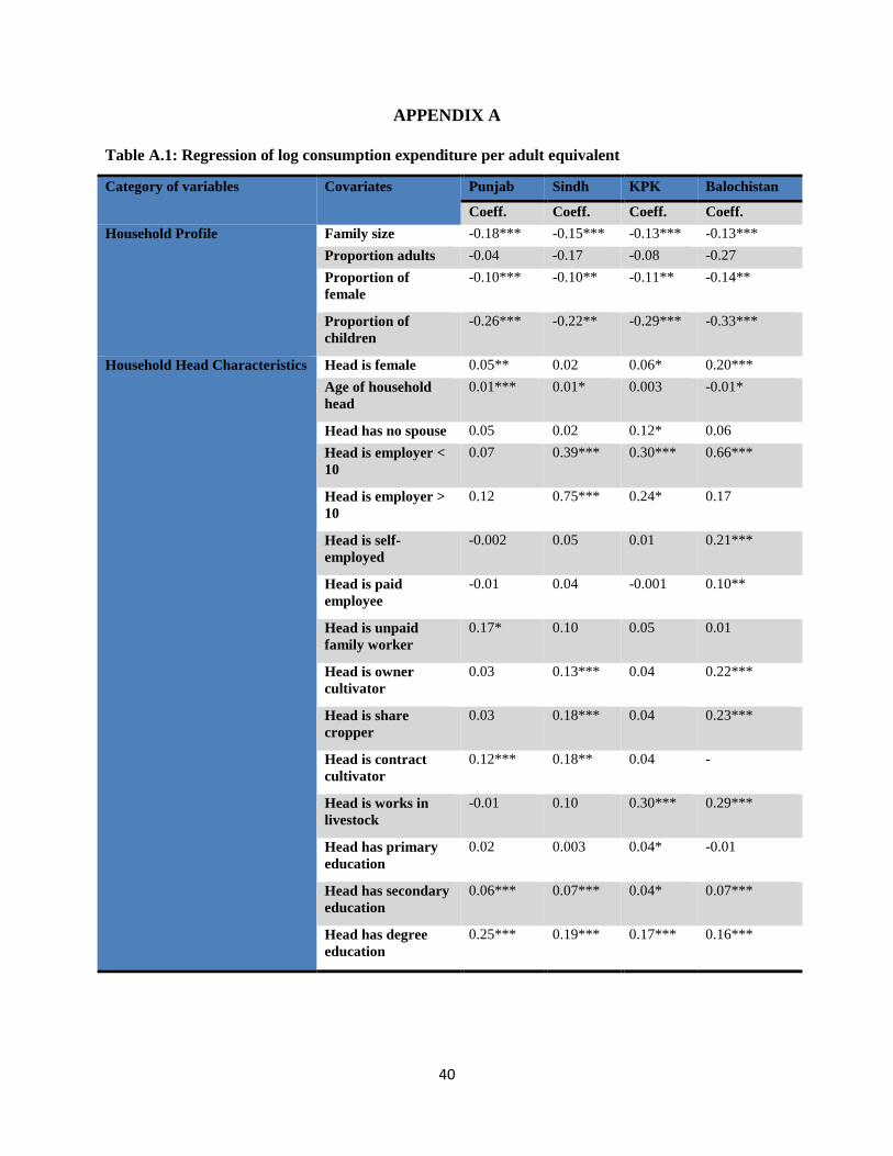
40

APPENDIX A

Table A.1: Regression of log consumption expenditure per adult equivalent

Category of variables Covariates Punjab Sindh KPK Balochistan

Coeff. Coeff. Coeff. Coeff.

Household Profile Family size -0.18*** -0.15*** -0.13*** -0.13***

Proportion adults -0.04 -0.17 -0.08 -0.27

Proportion of

female

-0.10*** -0.10** -0.11** -0.14**

Proportion of

children

-0.26*** -0.22** -0.29*** -0.33***

Household Head Characteristics Head is female 0.05** 0.02 0.06* 0.20***

Age of household

head

0.01*** 0.01* 0.003 -0.01*

Head has no spouse 0.05 0.02 0.12* 0.06

Head is employer <

10

0.07 0.39*** 0.30*** 0.66***

Head is employer >

10

0.12 0.75*** 0.24* 0.17

Head is self-

employed

-0.002 0.05 0.01 0.21***

Head is paid

employee

-0.01 0.04 -0.001 0.10**

Head is unpaid

family worker

0.17* 0.10 0.05 0.01

Head is owner

cultivator

0.03 0.13*** 0.04 0.22***

Head is share

cropper

0.03 0.18*** 0.04 0.23***

Head is contract

cultivator

0.12*** 0.18** 0.04 -

Head is works in

livestock

-0.01 0.10 0.30*** 0.29***

Head has primary

education

0.02 0.003 0.04* -0.01

Head has secondary

education

0.06*** 0.07*** 0.04* 0.07***

Head has degree

education

0.25*** 0.19*** 0.17*** 0.16***

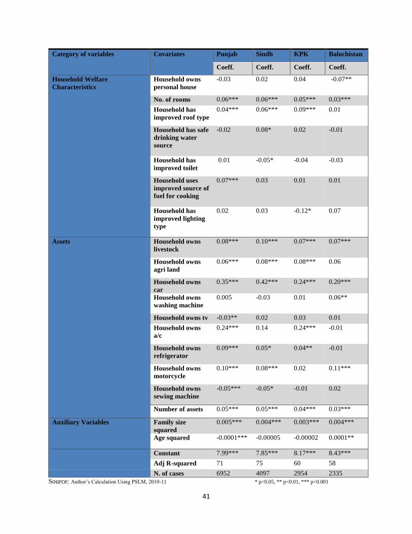
41

Category of variables Covariates Punjab Sindh KPK Balochistan

Coeff. Coeff. Coeff. Coeff.

Household Welfare

Characteristics

Household owns

personal house

-0.03 0.02 0.04 -0.07**

No. of rooms 0.06*** 0.06*** 0.05*** 0.03***

Household has

improved roof type

0.04*** 0.06*** 0.09*** 0.01

Household has safe

drinking water

source

-0.02 0.08* 0.02 -0.01

Household has

improved toilet

0.01 -0.05* -0.04 -0.03

Household uses

improved source of

fuel for cooking

0.07*** 0.03 0.01 0.01

Household has

improved lighting

type

0.02 0.03 -0.12* 0.07

Assets Household owns

livestock

0.08*** 0.10*** 0.07*** 0.07***

Household owns

agri land

0.06*** 0.08*** 0.08*** 0.06

Household owns

car

0.35*** 0.42*** 0.24*** 0.20***

Household owns

washing machine

0.005 -0.03 0.01 0.06**

Household owns tv -0.03** 0.02 0.03 0.01

Household owns

a/c

0.24*** 0.14 0.24*** -0.01

Household owns

refrigerator

0.09*** 0.05* 0.04** -0.01

Household owns

motorcycle

0.10*** 0.08*** 0.02 0.11***

Household owns

sewing machine

-0.05*** -0.05* -0.01 0.02

Number of assets 0.05*** 0.05*** 0.04*** 0.03***

Auxiliary Variables Family size

squared

0.005*** 0.004*** 0.003*** 0.004***

Age squared -0.0001*** -0.00005 -0.00002 0.0001**

Constant 7.99*** 7.85*** 8.17*** 8.43***

Adj R-squared 71 75 60 58

N. of cases 6952 4097 2954 2335

Source: Author’s Calculation Using PSLM, 2010-11 * p<0.05, ** p<0.01, *** p<0.001

42

Figure A.2a: Spatial Poverty Incidence-Punjab Unidimensional Poverty

Source: Author’s Calculation Using PSLM, 2010-11

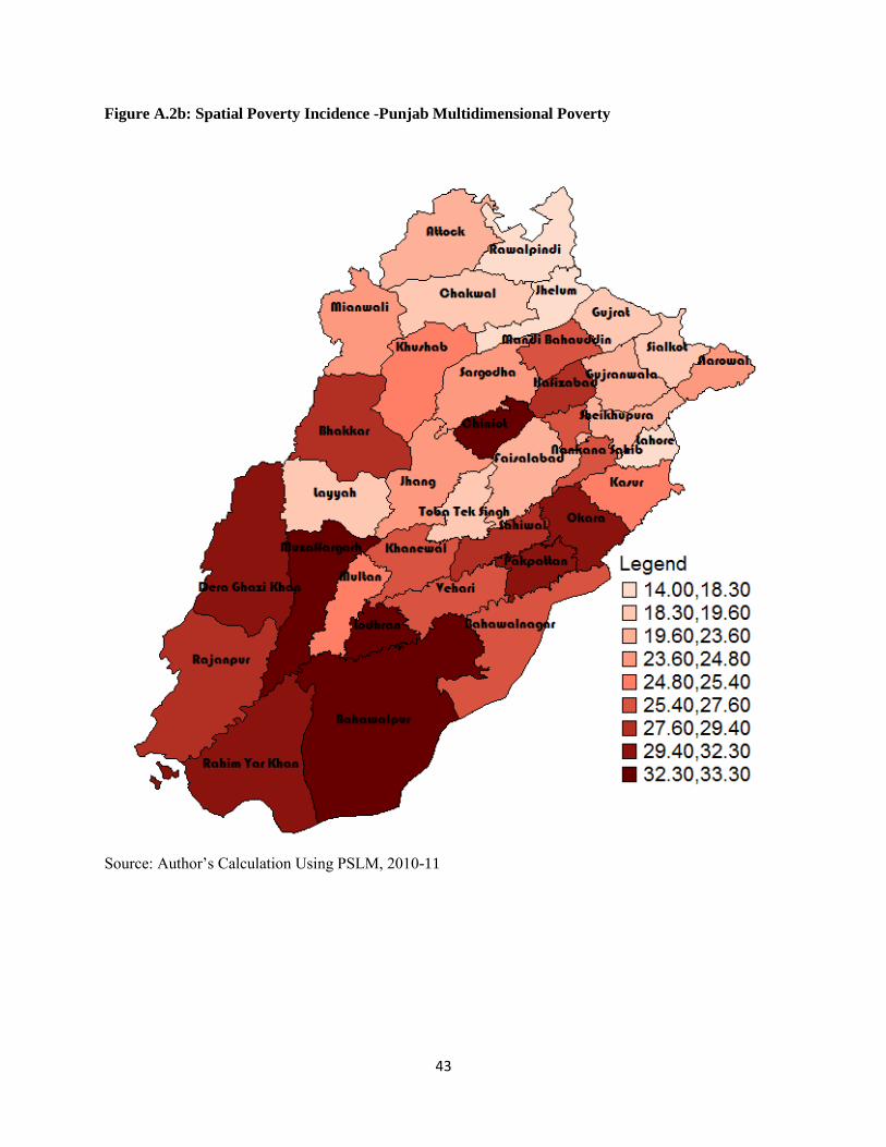
43

Figure A.2b: Spatial Poverty Incidence -Punjab Multidimensional Poverty

Source: Author’s Calculation Using PSLM, 2010-11

44

Figure A.3a: Spatial Poverty Incidence - Sindh Unidimensional Poverty

Source: Author’s Calculation Using PSLM, 2010-11

45

Figure A.3b: Spatial Poverty Incidence - Sindh Multidimensional Poverty

Source: Author’s Calculation Using PSLM, 2010-11

46

Figure A.4a: Spatial Poverty Incidence - KPK Unidimensional Poverty

Source: Author’s Calculation Using PSLM, 2010-11

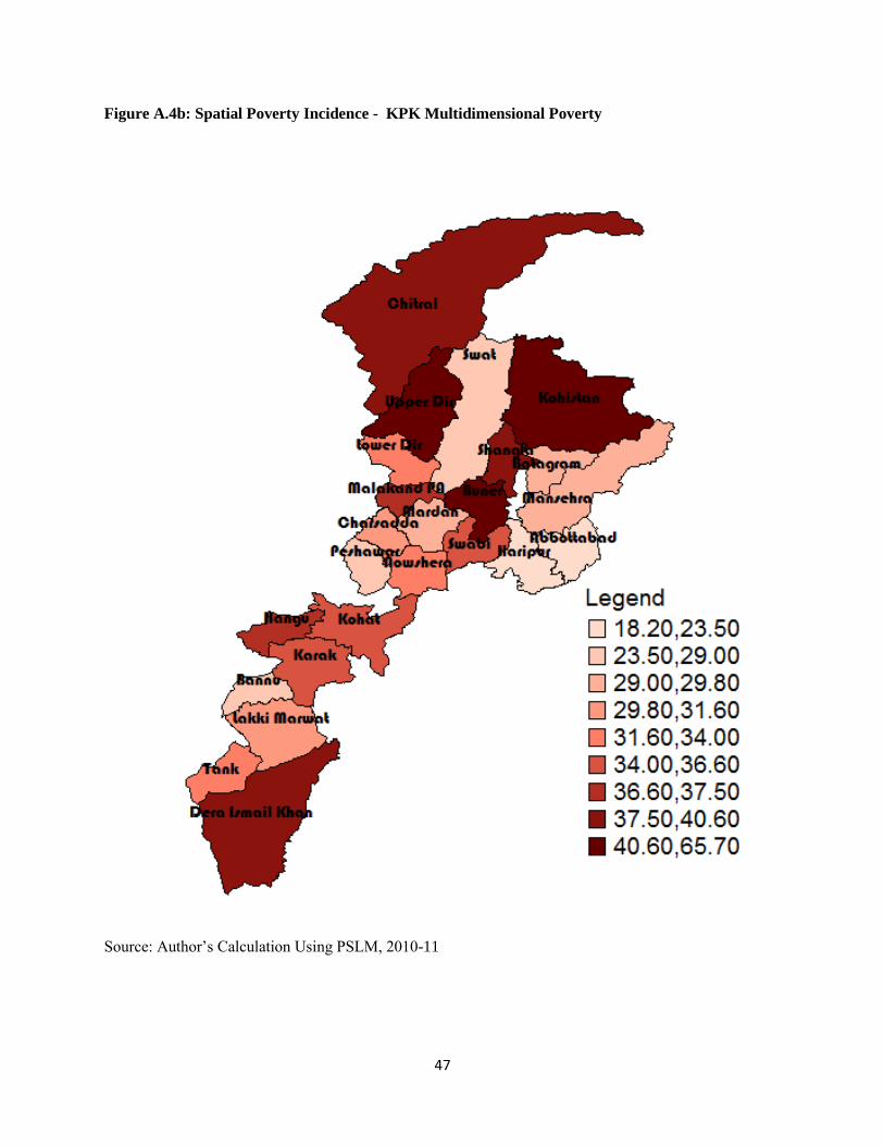
47

Figure A.4b: Spatial Poverty Incidence - KPK Multidimensional Poverty

Source: Author’s Calculation Using PSLM, 2010-11

48

Figure A.5a: Spatial Poverty Incidence - Balochistan Unidimensional Poverty

Source: Author’s Calculation Using PSLM, 2010-11

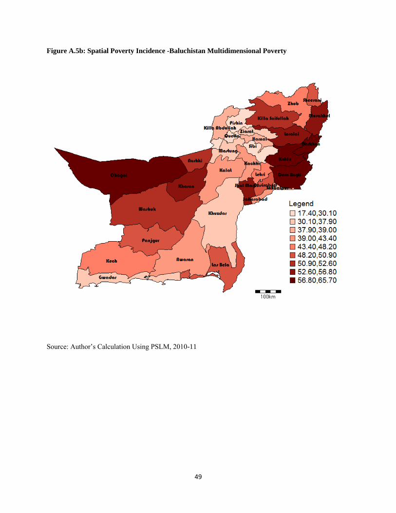
49

Figure A.5b: Spatial Poverty Incidence -Baluchistan Multidimensional Poverty

Source: Author’s Calculation Using PSLM, 2010-11

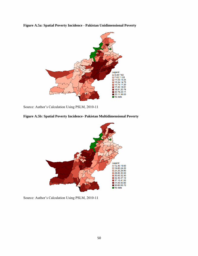
50

Figure A.5a: Spatial Poverty Incidence - Pakistan Unidimensional Poverty

Source: Author’s Calculation Using PSLM, 2010-11

Figure A.5b: Spatial Poverty Incidence- Pakistan Multidimensional Poverty

Source: Author’s Calculation Using PSLM, 2010-11

51

APPENDIX B

B.1: STATA do-file for Merging Covariates

Variable generation. do

cd "C:\pslm 10-11 hies\pslm 10-11 hies\hies data\data in stata\"

//demographics

use plist.dta, clear //the file includes information on household roster

gen age15=1 if age<15

replace age15=0 if age15==.

gen age65=1 if age>65

replace age65=0 if age65==.

gen hhsize=1

gen wrkng=1 if age>15 & age<65

replace wrkng =0 if wrkng ==.

gen nospouse=1 if idc==1 & sbq06==1

replace nospouse=0 if nospouse==.

gen child=1 if age<=12

replace child=0 if child==.

gen female=1 if sbq03==2

replace female=0 if female==.

gen agehh=age if idc==1

gen femalehh=1 if idc==1 & sbq03==2

replace femalehh=0 if femalehh==.

collapse (sum) femalehh agehh age15 age65 hhsize wrkng nospouse child female, by(hhcode)

gen dep=(age15+age65)/wrkng

gen female_prop=female/hhsize

gen child_prop=child/hhsize

gen prop_adults=age65/hhsize

save "C:\Users\shazia\Desktop\demographics.dta"

//education of head

use sec_c.dta, clear // the file contains data about education of household roster

drop if idc!=1 //since household head’s education is used, the rest of the roster is dropped

gen educ=scq04

replace educ=7 if educ==17 //diploma label of 17 is changed to 7 so as to relabel it as secondary

recode educ (1/6=1) (7/12=2) (12/max=3)

label define e 0 "illiterate" 1 "primary" 2 "secondary" 3 "degree

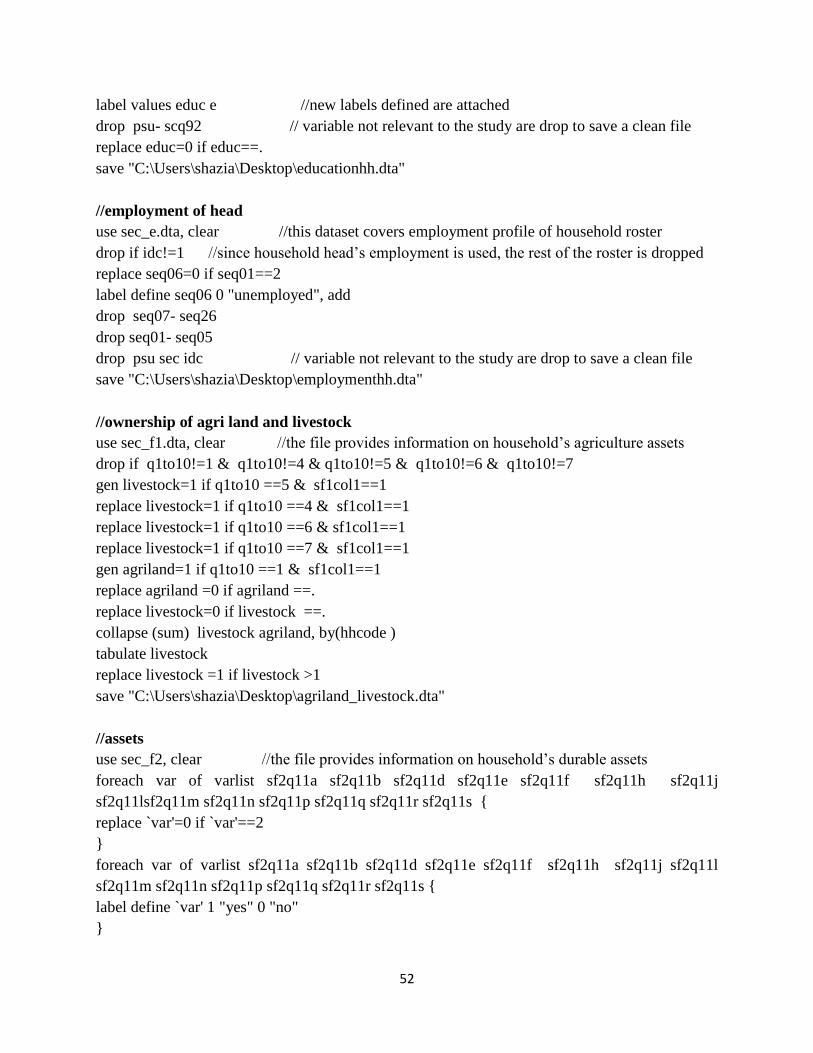
52

label values educ e //new labels defined are attached

drop psu- scq92 // variable not relevant to the study are drop to save a clean file

replace educ=0 if educ==.

save "C:\Users\shazia\Desktop\educationhh.dta"

//employment of head

use sec_e.dta, clear //this dataset covers employment profile of household roster

drop if idc!=1 //since household head’s employment is used, the rest of the roster is dropped

replace seq06=0 if seq01==2

label define seq06 0 "unemployed", add

drop seq07- seq26

drop seq01- seq05

drop psu sec idc // variable not relevant to the study are drop to save a clean file

save "C:\Users\shazia\Desktop\employmenthh.dta"

//ownership of agri land and livestock

use sec_f1.dta, clear //the file provides information on household’s agriculture assets

drop if q1to10!=1 & q1to10!=4 & q1to10!=5 & q1to10!=6 & q1to10!=7

gen livestock=1 if q1to10 ==5 & sf1col1==1

replace livestock=1 if q1to10 ==4 & sf1col1==1

replace livestock=1 if q1to10 ==6 & sf1col1==1

replace livestock=1 if q1to10 ==7 & sf1col1==1

gen agriland=1 if q1to10 ==1 & sf1col1==1

replace agriland =0 if agriland ==.

replace livestock=0 if livestock ==.

collapse (sum) livestock agriland, by(hhcode )

tabulate livestock

replace livestock =1 if livestock >1

save "C:\Users\shazia\Desktop\agriland_livestock.dta"

//assets

use sec_f2, clear //the file provides information on household’s durable assets

foreach var of varlist sf2q11a sf2q11b sf2q11d sf2q11e sf2q11f sf2q11h sf2q11j

sf2q11lsf2q11m sf2q11n sf2q11p sf2q11q sf2q11r sf2q11s {

replace `var'=0 if `var'==2

}

foreach var of varlist sf2q11a sf2q11b sf2q11d sf2q11e sf2q11f sf2q11h sf2q11j sf2q11l

sf2q11m sf2q11n sf2q11p sf2q11q sf2q11r sf2q11s {

label define `var' 1 "yes" 0 "no"

}

53

gen assets=0

foreach var of varlist sf2q11a sf2q11b sf2q11d sf2q11e sf2q11f sf2q11h sf2q11j

sf2q11lsf2q11m sf2q11n sf2q11p sf2q11q sf2q11r sf2q11s {

replace assets = assets+`var'

}

gen tv=1 if sf2q11g==1

replace tv=0 if tv==.

gen ac=1 if sf2q11k==1

replace ac=0 if ac==.

gen washing_mach=1 if sf2q11t==1

replace washing_mach =0 if washing_mach ==.

gen motorcycle=1 if sf2q11n==1

replace motorcycle =0 if motorcycle ==.

gen sewing_mach=1 if sf2q11c==1

replace sewing_mach =0 if sewing_mach ==.

gen refrigerator=1 if sf2q11i==1

replace refrigerator =0 if refrigerator ==.

drop psu section sf2q11a sf2q11b sf2q11c sf2q11d sf2q11e sf2q11f sf2q11g sf2q11h sf2q11i

sf2q11j sf2q11k sf2q11l sf2q11m sf2q11n sf2q11o sf2q11p sf2q11q sf2q11r sf2q11s sf2q11t

sf2q12 sf2q13

save "C:\Users\shazia\Desktop\number of assets.dta"

//household characteristics

use sec_g, clear //file gives information on household’s non-income welfare characteristics

recode sgq01 (1=1) (2=1) (5=1) (3=0) (4=0)

label define sgq01 1 "ownership" 0 "no ownship", modify

recode sgq03 (1=1) (3=1) (4=1) (2=0)

label define sgq03 1 "improved" 0 "not improved", modify

recode sgq05 (1/5=1) (8/9=1) (6/7=0) (10=0)

label define sgq05 1 "safe" 0 "notsafe", modify

recode sgq06 (2/3=1) (6=1) (1=0) (4/5=0) (7=0)

label define sgq06 1 "improved" 0 "not improved", modify

recode sgq08 (1/3=1) (4/6=0)

label define sgq08 1 "improved" 0 "not improved", modify

recode sgq07 (2/5=1) (1=0) (6/8=0)

label define sgq07 1 "improved" 0 "not improved", modify

drop sgq09 sgq10a1 sgq10a2 sgq10b1 sgq10b2 sgq10c1 sgq10c2 sgq10d1 sgq10d2 sgq10e1

sgq10e2 sgq10f1 sgq10f2 sgq10g1 sgq10g2 sgq10h1 sgq10h2

rename sgq01 ownrship

rename sgq02 no_rooms

54

rename sgq03 roof

drop sgq04

rename sgq05 water

rename sgq06 toilet

rename sgq07 cooking

rename sgq08 lighting

drop psu section

save "C:\Users\shazia\Desktop\non_income indicators.dta"

//merge

cd "c:\users\shazia\desktop\"

use demographics.dta, clear

merge 1:1 hhcode using "C:\Users\Shazia\Desktop\educationhh.dta"

drop if _merge!=3

drop _merge

merge 1:1 hhcode using "C:\Users\Shazia\Desktop\employmenthh.dta"

drop if _merge!=3

drop _merge

merge 1:1 hhcode using "C:\Users\Shazia\Desktop\agriland_livestock.dta"

drop if _merge!=3

drop _merge

merge 1:1 hhcode using "C:\Users\Shazia\Desktop\number of assets.dta"

drop if _merge!=3

drop _merge

merge 1:1 hhcode using "C:\Users\Shazia\Desktop\non_income indicators.dta"

drop if _merge!=3

drop _merge

tabulate educ, gen(educ) //to generate dummy variables for each type of education

xi i.seq06 //to generate dummy variables of each employment type

save "C:\Users\shazia\Desktop\sheet.dta"

B.2: STATA do-file for Consumption calculation

Consumption calculation.do

use sec6abcde.dta, clear //detailed consumption expenditures are provided in this file

foreach var of varlist v1 v2 v3 v4 {

replace `var'=`var'/12 if itc>=5101 & itc<=5406 //expenditure are adjusted to monthly scale from

annually

replace `var'=`var'/12 if itc>=5408 & itc<=5701

replace `var'=`var'/12 if itc>=5705 & itc<=5804

55

replace `var'=`var'/12 if itc>=5902 & itc<=5904

replace `var'=`var'/12 if itc>=6501 & itc<=6504

replace `var'=`var'*2.17 if itc>=1101 & itc<=1901 //expenditure are adjusted to monthly scale

from fortnightly

replace `var'=`var'/12 if itc==6101

}

keep if itc>=1101 & itc<=1901 | itc>=2101 & itc<=3003 | itc>=4101 & itc<=4406 | itc>=5101 &

itc<=5406 | itc>=5408 & itc<=5701 | itc>=5705 & itc<=5804 | itc>=5902 & itc<=5904 |

itc>=6501 & itc<=6504 | itc==6101 //the relevant codes of consumption components are kept

while dropping others.

collapse (sum) v1 v2 v3 v4, by(hhcode )

gen cons=v1+v2+v3+v4 //consumption

save "C:\Users\shazia\Desktop\consumption.dta"

B.3: STATA do-file for adult equivalent household size and consumption expenditure per

adult equivalent

Adult equivalent hhsize & consumption per adulteq.do

use plist.dta, clear // data on household roster

gen child=1 if age<=12 //assigns a value of 1 to members less than or equal to 12 years of age

replace child =0 if child==. //inserts zero where household member is greater than 12

gen hhsize=1

collapse (sum) child hhsize , by(hhcode )

gen adult=hhsize-child //number of adults are found by subtracting number of children from

hhsize

replace child=child*0.8 //children are given weight of 0.8

gen hhsize_adultequiv=adult+child //redefined number of children are added to number of adults

for hhsize

keep hhsize hhcode hhsize_adultequiv

save "C:\Users\shazia\Desktop\hhsize_adult.dta"

//adult equivalent hhsize merged with monthly consumption expenditure

//merge

cd "c:\users\shazia\desktop\"

use consumption.dta, clear //calculated monthly consumption expenditure

merge 1:1 hhcode using "C:\Users\Shazia\Desktop\hhsize_adult.dta"

drop if _merge!=3

drop _merge

gen per_adeqcons=cons/hhsize_adultequiv //consumption expenditure divided by adult

equivalent hhsize

merge 1:1 hhcode using "C:\Users\Shazia\Desktop\sheet.dta"

56

drop if _merge!=3

drop _merge

gen lpc=ln(per_adeqcons) // log of consumption expenditure per adult equivalent

save "C:\Users\shazia\Desktop\sheet.dta, replace"

B.4 STATA do-file for poverty estimation at district level using SAE

SAE.do

cd "C:\Users\shazia\Desktop\shazia\files\"

use sheet.dta //file including all covariates and log of adult equivalent consumption expenditure

svyset psu [pweight = weight], strata(province) // declaring survey data

forval i=1/4 {

svy: reg lpc hhsize nospouse prop_adults female_prop child_prop livestock agriland assets

ownrship no_rooms roof water toilet cooking lighting car washing_mach tv ac refrigerator

motorcycle sewing_mach hhsizesq age femalehh agesq _Iseq06_1 _Iseq06_2 _Iseq06_3

_Iseq06_4 _Iseq06_5 _Iseq06_6 _Iseq06_7 _Iseq06_8 _Iseq06_9 educ2 educ3 educ4 if province

==`i'

mat beta`i' = e(b)

predict e`i', residual // predicting residuals for each province to standard error calculation

replace e`i' = (e`i')^2

}

replace e1=. if province!=1 //inserting a missing value operator “.” So as to estimate sum of

squared residuals using only province specific values.

replace e2=. if province!=2

replace e3=. if province!=3

replace e4=. if province!=4

forval i=1/4 {

summarize e`i'

gen se`i'=r(sum)

}

replace se1=. if province!=1

replace se2=. if province!=2

replace se3=. if province!=3

replace se4=. if province!=4

replace se1=se1/6915 //the number of observation for punjab is adjusted for degree of freedoms.

replace se2=se2/4059 //the number of observation for sind is adjusted for degree of freedoms.

replace se3=se3/2915//the number of observation for kpk is adjusted for degree of freedoms.

replace se4=se4/2295//the number of observation for balochistan is adjusted for degree of

freedoms.

forval i=1/4 {

57

replace se`i'=(se`i')^0.5

}

summarize se1

gen se11=r(mean)

summarize se2

gen se12=r(mean)

summarize se3

gen se13=r(mean)

summarize se4

gen se14=r(mean)

forval i=1/4 {

svmat double beta`i'

}

keep se11 - beta439

drop if beta11==.

expand 76527

save "C:\Users\shazia\Desktop\betas.dta"

use district_sheet.dta, clear

merge 1:1 _n using "C:\Users\shazia\Desktop\betas.dta"

gen lpreg=0

forval i=1/4 {

gen lpren`i' = beta`i'27*_Iseq06_1 + beta`i'28*_Iseq06_2 + beta`i'29*_Iseq06_3 +

beta`i'30*_Iseq06_4 + beta`i'31*_Iseq06_5 + beta`i'32*_Iseq06_6 + beta`i'33*_Iseq06_7 +

beta`i'34*_Iseq06_8 + beta`i'35*_Iseq06_9 + beta`i'36*educ2 + beta`i'37*educ3 +

beta`i'38*educ4 + beta`i'1*hhsize + beta`i'2*nospouse + beta`i'3*prop_adults+

beta`i'4*female_prop + beta`i'5* child_prop + beta`i'6*livestock + beta`i'7*agriland +

beta`i'8*assets + beta`i'9*ownership + beta`i'10*no_rooms+ beta`i'11*roof + beta`i'12*water+

beta`i'13*toilet + beta`i'14*cooking + beta`i'15*lighting + beta`i'16*car +

beta`i'17*washing_mach+ beta`i'18*tv + beta`i'19* ac + beta`i'20*refrigerator +

beta`i'21*motorcycle + beta`i'22*sewing_mach + beta`i'23*hhsizesq + beta`i'24*age +

beta`i'25*femalehh + beta`i'26*agesq + beta`i'39 if province==`i'

replace lpren`i' = 0 if lpren`i'==.

replace lpreg = lpreg + lpren`i'

}

forval i=11/14 {

gen z`i' = (7.4645-lpreg)/se`i' //z-score measurement

}

replace z11=0 if province!=1

replace z12=0 if province!=2

replace z13=0 if province!=3

58

replace z14=0 if province!=4

gen z=0

forval i =11/14 {

replace z`i'=0 if z`i'==.

replace z=z+z`i'

}

gen probabilities=normal(z) //estimating of probabilities using cumulative normal distribution

mean probabilities, over(district) //calculation of poverty as average of probabilities over each

district.

B.5 STATA do-file for preparing variables and measuring multidimensional poverty

MDP.do

cd “c:\users\shazia\desktop\plsm2010-11\data in stata\”

use sec G.dta, clear //PLSM file for non-income welfare indicators of households.

recode sgq01 (1=1) (2=1) (5=1) (3=0) (4=0)

label define sgq01 1 "ownership" 0 "no ownship", modify

recode sgq03 (1=1) (3=1) (4=1) (2=0)

label define sgq03 1 "improved" 0 "not improved", modify

recode sgq05 (1/5=1) (8/9=1) (6/7=0) (10=0)

label define sgq05 1 "safe" 0 "notsafe", modify

recode sgq06 (2/3=1) (6=1) (1=0) (6=0) (4=0) (7=0)

label define sgq06 1 "improved" 0 "not improved", modify

recode sgq08 (1/3=1) (4/6=0)

label define sgq08 1 "improved" 0 "not improved", modify

recode sgq07 (2/3=1) (5=1) (4=0) (1=0) (6/8=0)

label define sgq07 1 "improved" 0 "not improved", modify

drop sgq09 sgq10a1 sgq10a2 sgq10b1 sgq10b2 sgq10c1 sgq10c2 sgq10d1 sgq10d2 sgq10e1

sgq10e2 sgq10f1 sgq10f2 sgq10g1 sgq10g2 sgq10h1 sgq10h2

rename sgq01 ownrship

rename sgq03 roof

drop sgq04

rename sgq05 water

rename sgq06 toilet

rename sgq07 cooking

rename sgq08 lighting

drop psu section

save "C:\Users\shazia\Desktop\non_income indicators.dta"

cd “c:\users\shazia\desktop\plsm2010-11\data in stata\”

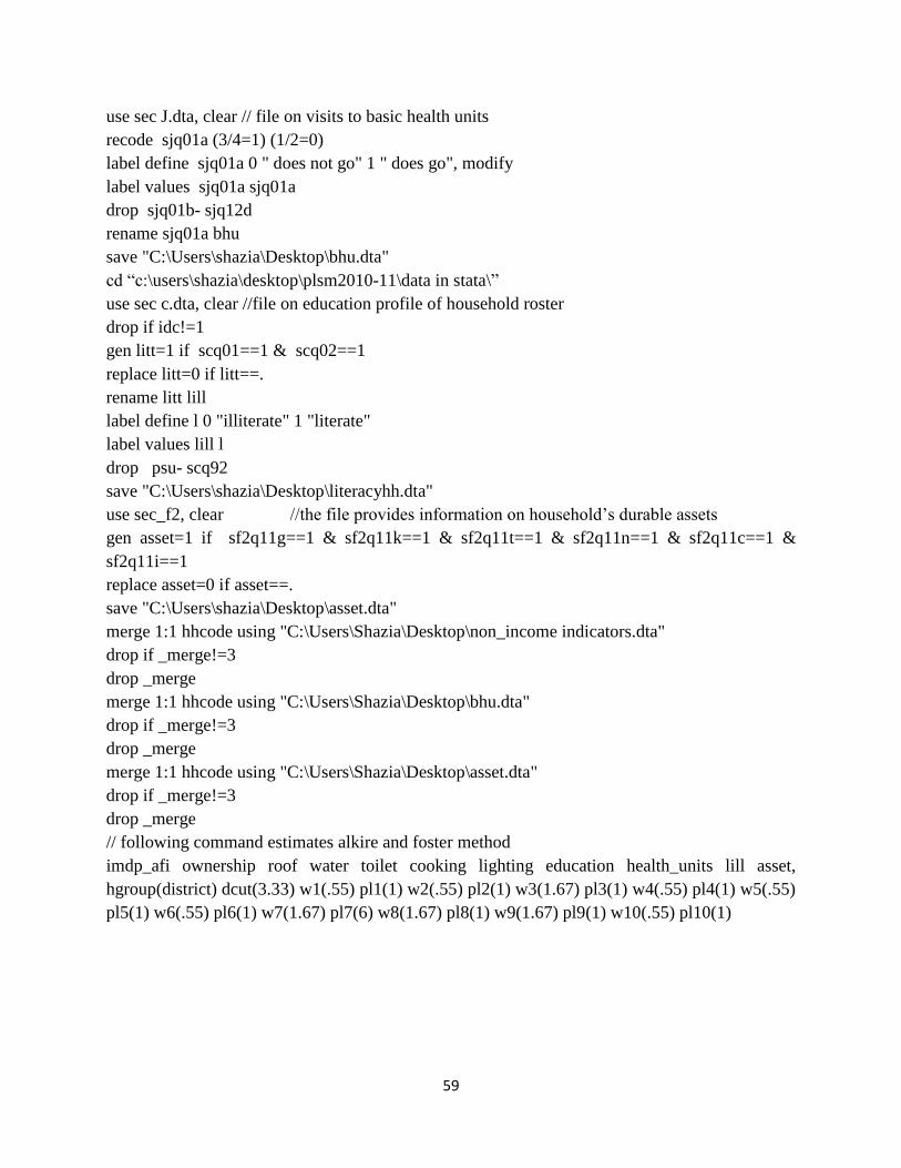
59

use sec J.dta, clear // file on visits to basic health units

recode sjq01a (3/4=1) (1/2=0)

label define sjq01a 0 " does not go" 1 " does go", modify

label values sjq01a sjq01a

drop sjq01b- sjq12d

rename sjq01a bhu

save "C:\Users\shazia\Desktop\bhu.dta"

cd “c:\users\shazia\desktop\plsm2010-11\data in stata\”

use sec c.dta, clear //file on education profile of household roster

drop if idc!=1

gen litt=1 if scq01==1 & scq02==1

replace litt=0 if litt==.

rename litt lill

label define l 0 "illiterate" 1 "literate"

label values lill l

drop psu- scq92

save "C:\Users\shazia\Desktop\literacyhh.dta"

use sec_f2, clear //the file provides information on household’s durable assets

gen asset=1 if sf2q11g==1 & sf2q11k==1 & sf2q11t==1 & sf2q11n==1 & sf2q11c==1 &

sf2q11i==1

replace asset=0 if asset==.

save "C:\Users\shazia\Desktop\asset.dta"

merge 1:1 hhcode using "C:\Users\Shazia\Desktop\non_income indicators.dta"

drop if _merge!=3

drop _merge

merge 1:1 hhcode using "C:\Users\Shazia\Desktop\bhu.dta"

drop if _merge!=3

drop _merge

merge 1:1 hhcode using "C:\Users\Shazia\Desktop\asset.dta"

drop if _merge!=3

drop _merge

// following command estimates alkire and foster method

imdp_afi ownership roof water toilet cooking lighting education health_units lill asset,

hgroup(district) dcut(3.33) w1(.55) pl1(1) w2(.55) pl2(1) w3(1.67) pl3(1) w4(.55) pl4(1) w5(.55)

pl5(1) w6(.55) pl6(1) w7(1.67) pl7(6) w8(1.67) pl8(1) w9(1.67) pl9(1) w10(.55) pl10(1)

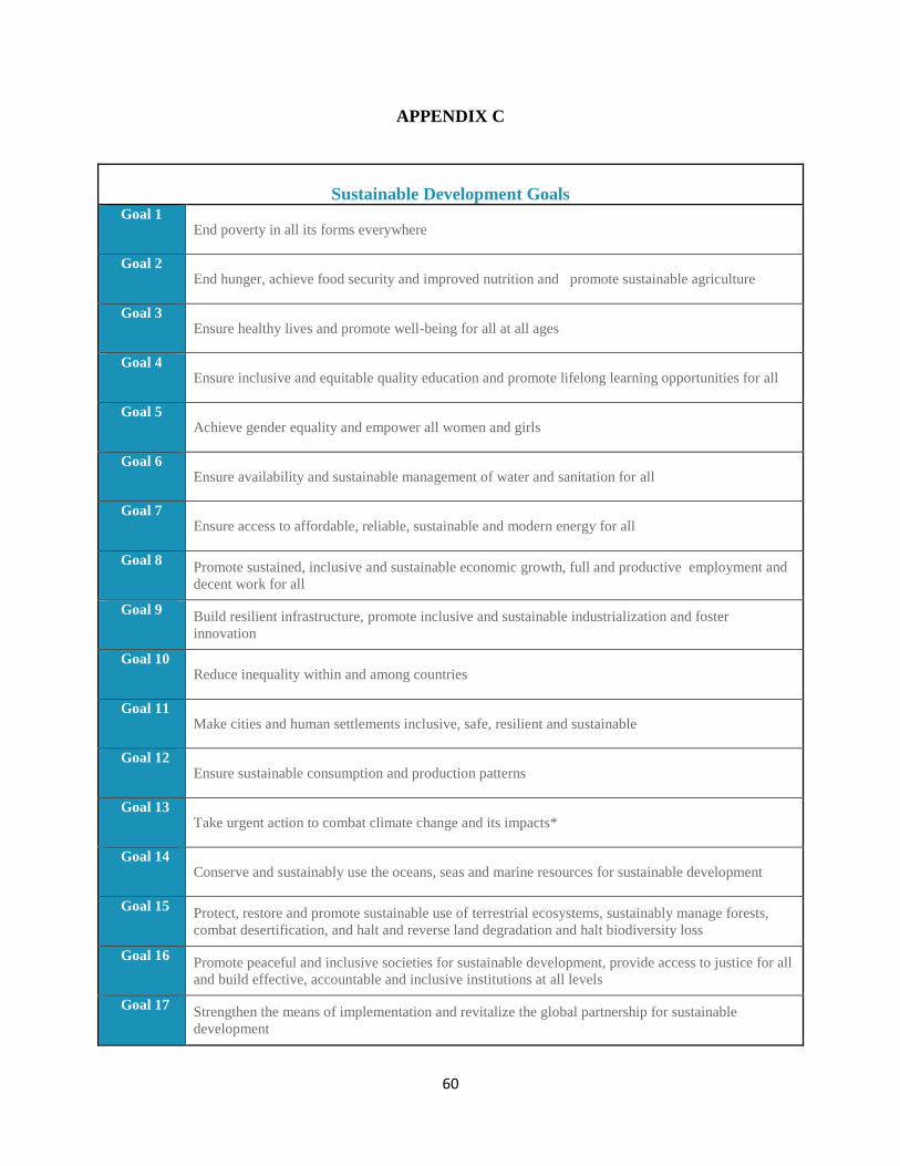
60

APPENDIX C

Sustainable Development Goals Goal 1

End poverty in all its forms everywhere

Goal 2 End hunger, achieve food security and improved nutrition and promote sustainable agriculture

Goal 3 Ensure healthy lives and promote well-being for all at all ages

Goal 4 Ensure inclusive and equitable quality education and promote lifelong learning opportunities for all

Goal 5 Achieve gender equality and empower all women and girls

Goal 6 Ensure availability and sustainable management of water and sanitation for all

Goal 7 Ensure access to affordable, reliable, sustainable and modern energy for all

Goal 8 Promote sustained, inclusive and sustainable economic growth, full and productive employment and

decent work for all

Goal 9 Build resilient infrastructure, promote inclusive and sustainable industrialization and foster

innovation

Goal 10 Reduce inequality within and among countries

Goal 11 Make cities and human settlements inclusive, safe, resilient and sustainable

Goal 12 Ensure sustainable consumption and production patterns

Goal 13 Take urgent action to combat climate change and its impacts*

Goal 14 Conserve and sustainably use the oceans, seas and marine resources for sustainable development

Goal 15 Protect, restore and promote sustainable use of terrestrial ecosystems, sustainably manage forests,

combat desertification, and halt and reverse land degradation and halt biodiversity loss

Goal 16 Promote peaceful and inclusive societies for sustainable development, provide access to justice for all

and build effective, accountable and inclusive institutions at all levels

Goal 17 Strengthen the means of implementation and revitalize the global partnership for sustainable

development

61

Millennium Development Goals (MDGs)

Goals and Targets

(from the Millennium Declaration)

Indicators for monitoring progress

Goal 1: Eradicate extreme poverty and hunger

Target 1.A: Halve, between 1990 and 2015, the proportion of people whose

income is less than one dollar a day

1.1 Proportion of population below $1.25 (PPP) per dayi 1.2 Poverty gap ratio 1.3 Share of poorest quintile in national consumption

Target 1.B: Achieve full and productive employment and decent work for all,

including women and young people

1.4 Growth rate of GDP per person employed 1.5 Employment-to-population ratio 1.6 Proportion of employed people living below $1.25 (PPP) per day 1.7 Proportion of own-account and contributing family workers in total

employment

Target 1.C: Halve, between 1990 and 2015, the proportion of

people who suffer from hunger

1.8 Prevalence of underweight children under-five years of age 1.9 Proportion of population below minimum level of dietary energy

consumption

Goal 2: Achieve universal primary education

Target 2.A: Ensure that, by 2015, children everywhere, boys and girls alike,

will be able to complete a full course of primary schooling

2.1 Net enrolment ratio in primary education 2.2 Proportion of pupils starting grade 1 who reach last grade of primary 2.3 Literacy rate of 15-24 year-olds, women and men

Goal 3: Promote gender equality and empower women

Target 3.A: Eliminate gender disparity in primary and secondary education,

preferably by 2005, and in all levels of education no later than 2015

3.1 Ratios of girls to boys in primary, secondary and tertiary education 3.2 Share of women in wage employment in the non-agricultural sector 3.3 Proportion of seats held by women in national parliament

Goal 4: Reduce child mortality

Target 4.A: Reduce by two-thirds, between 1990 and 2015, the under-five

mortality rate

4.1 Under-five mortality rate 4.2 Infant mortality rate 4.3 Proportion of 1 year-old children immunised against measles

Goal 5: Improve maternal health

Target 5.A: Reduce by three quarters, between 1990 and 2015, the maternal

mortality ratio

5.1 Maternal mortality ratio 5.2 Proportion of births attended by skilled health personnel

Target 5.B: Achieve, by 2015, universal access to reproductive health

5.3 Contraceptive prevalence rate 5.4 Adolescent birth rate 5.5 Antenatal care coverage (at least one visit and at least four visits) 5.6 Unmet need for family planning

Goal 6: Combat HIV/AIDS, malaria and other diseases

Target 6.A: Have halted by 2015 and begun to reverse the spread of

HIV/AIDS

6.1 HIV prevalence among population aged 15-24 years

6.2 Condom use at last high-risk sex

6.3 Proportion of population aged 15-24 years with comprehensive correct

knowledge of HIV/AIDS

6.4 Ratio of school attendance of orphans to school attendance of non-

orphans aged 10-14 years

62

Target 6.B: Achieve, by 2010, universal access to treatment for HIV/AIDS for

all those who need it

6.5 Proportion of population with advanced HIV infection with access to antiretroviral drugs

Target 6.C: Have halted by 2015 and begun to reverse the incidence of

malaria and other major diseases

6.6 Incidence and death rates associated with malaria 6.7 Proportion of children under 5 sleeping under insecticide-treated

bednets 6.8 Proportion of children under 5 with fever who are treated with

appropriate anti-malarial drugs 6.9 Incidence, prevalence and death rates associated with tuberculosis 6.10 Proportion of tuberculosis cases detected and cured under directly

observed treatment short course

Goal 7: Ensure environmental sustainability

Target 7.A: Integrate the principles of sustainable development into country

policies and programmes and reverse the loss of environmental resources

Target 7.B: Reduce biodiversity loss, achieving, by 2010, a significant

reduction in the rate of loss

7.1 Proportion of land area covered by forest 7.2 CO2 emissions, total, per capita and per $1 GDP (PPP) 7.3 Consumption of ozone-depleting substances 7.4 Proportion of fish stocks within safe biological limits 7.5 Proportion of total water resources used 7.6 Proportion of terrestrial and marine areas protected 7.7 Proportion of species threatened with extinction

Target 7.C: Halve, by 2015, the proportion of people without sustainable

access to safe drinking water and basic sanitation

7.8 Proportion of population using an improved drinking water source 7.9 Proportion of population using an improved sanitation facility

Target 7.D: By 2020, to have achieved a significant improvement in the lives

of at least 100 million slum dwellers

7.10 Proportion of urban population living in slumsii

Goal 8: Develop a global partnership for development

Target 8.A: Develop further an open, rule-based, predictable, non-

discriminatory trading and financial system

Includes a commitment to good governance, development and poverty

reduction – both nationally and internationally

Target 8.B: Address the special needs of the least developed countries

Includes: tariff and quota free access for the least developed countries'

exports; enhanced programme of debt relief for heavily indebted poor

countries (HIPC) and cancellation of official bilateral debt; and more generous

ODA for countries committed to poverty reduction

Some of the indicators listed below are monitored separately for the least

developed countries (LDCs), Africa, landlocked developing countries and

small island developing States.

Official development assistance (ODA)

8.1 Net ODA, total and to the least developed countries, as percentage of OECD/DAC donors’ gross national income

8.2 Proportion of total bilateral, sector-allocable ODA of OECD/DAC donors to basic social services (basic education, primary health care, nutrition, safe water and sanitation)

8.3 Proportion of bilateral official development assistance of OECD/DAC donors that is untied

8.4 ODA received in landlocked developing countries as a proportion of their gross national incomes

8.5 ODA received in small island developing States as a proportion of their gross national incomes

Market access

8.6 Proportion of total developed country imports (by value and excluding arms) from developing countries and least developed countries, admitted free of duty

63

Target 8.C: Address the special needs of landlocked developing countries and

small island developing States (through the Programme of Action for the

Sustainable Development of Small Island Developing States and the outcome

of the twenty-second special session of the General Assembly)

Target 8.D: Deal comprehensively with the debt problems of developing

countries through national and international measures in order to make debt

sustainable in the long term

8.7 Average tariffs imposed by developed countries on agricultural products and textiles and clothing from developing countries

8.8 Agricultural support estimate for OECD countries as a percentage of their gross domestic product

8.9 Proportion of ODA provided to help build trade capacity Debt sustainability

8.10 Total number of countries that have reached their HIPC decision points and number that have reached their HIPC completion points (cumulative)

8.11 Debt relief committed under HIPC and MDRI Initiatives 8.12 Debt service as a percentage of exports of goods and services

Target 8.E: In cooperation with pharmaceutical companies, provide access to

affordable essential drugs in developing countries

8.13 Proportion of population with access to affordable essential drugs on a sustainable basis

Target 8.F: In cooperation with the private sector, make available the benefits

of new technologies, especially information and communications

8.14 Fixed-telephone subscriptions per 100 inhabitants 8.15 Mobile-cellular subscriptions per 100 inhabitants 8.16 Internet users per 100 inhabitants

The Millennium Development Goals and targets come from the Millennium Declaration, signed by 189 countries, including 147 heads of State and Government, in September 2000

(http://www.un.org/millennium/declaration/ares552e.htm) and from further agreement by member states at the 2005 World Summit (Resolution adopted by the General Assembly -

A/RES/60/1, http://www.un.org/Docs/journal/asp/ws.asp?m=A/RES/60/1). The goals and targets are interrelated and should be seen as a whole. They represent a partnership between

the developed countries and the developing countries “to create an environment – at the national and global levels alike – which is conducive to development and the elimination of

poverty”.

i For monitoring country poverty trends, indicators based on national poverty lines should be used, where available. ii The actual proportion of people living in slums is measured by a proxy, represented by the urban population living in households with at least one of the four characteristics: (a) lack of access to improved water supply; (b) lack of access to improved sanitation; (c) overcrowding (3 or more persons per room); and (d) dwellings made of non-durable material.