Embed Size (px)
Citation preview

^ September 1985 Report No. STAN-CS-85-1069
PB96-149620
The Logical Data Model: A New Approach
To Database Logic
by
Gabriel Mark Kupcr
toe ̂ ^AllTy ^^c^^
Department of Computer Science
Stanford University Stanford, CA 94305
19970422 040

1
THE LOGICAL DATA MODEL:
A NEW APPROACH
TO DATABASE LOGIC
A DISSERTATION
SUBMITTED TO THE DEPARTMENT OF COMPUTER SCIENCE
AND THE COMMITTEE ON GRADUATE STUDIES
OF STANFORD UNIVERSITY
IN PARTIAL FULFILLMENT OF THE REQUIREMENTS FOR THE DEGREE OF
DOCTOR OF PHILOSOPHY
By Gabriel Mark Kuper
September 1985

© Copyright 1985 by
Gabriel Mark Kuper

I certify that I have read this thesis and that in my opinion it is fully adequate, in scope and in quality, as a dissertation for the degree of Doctor of Philosophy.
Jeffrey D. Ullman (Principal Adviser)
I certify that I have read this thesis and that in my opinion it is fully adequate, in scope and in quality, as a dissertation for the degree of Doctor of Philosophy.
Christos H. Papadimitriou
I certify that I have read this thesis and that in my opinion it is fully adequate, in scope and in quality, as a dissertation for the degree of Doctor of Philosophy.
Moshe Y. Vardi (CSLI)
Approved for the University Committee on Graduate Studies:
Dean of Graduate Studies & Research
111
Abstract
We propose a mathematical framework for unifying and generalizing the principal data models i e the relational, hierarchical and network models. Until recently most theoretical work on databases has focused on the relational model, mainly due to its elegance and mathematical simplicity compared to the other models. Some of this work has pointed out various disadvantages of the relational model, among them its lack of semantics and the fact that it forces the data to have a flat structure that the real data does not always have.
The Logical Data Model (LDM) combines the advantages of the relational, network and hierarchical approaches. It models database Schemas as directed graphs, in which the leaves correspond to the attributes and the internal nodes to connections between the data. Instances of LDM Schemas consist of r-values which constitute the data space, and 1-values, which constitute the address space. We are thus able to deal with instances of cyclic structures, but still get a first-order theory.
We define a logic on LDM schemas in which integrity constraints can be specified, and use it to define a logical, i.e., non-procedural, query language that is analogous to Codd's relational calculus. We also describe an algebraic, i.e., procedural, query language and prove that the two languages are equivalent Inese languages have a novel feature: not only can they access a non-flat data structure, e.g. a hierarchy but the answers they produce do not have to be flat either. Thus, the language really does have the ability to restructure data and not only to retrieve it, and can therefore be used both as a query language and for defining views.
IV

Acknowledgments
I would like to especially thank my adviser, Jeff Ullman. He both suggested this area as a good one for research, and was very helpful in advising me which directions to explore. I would like to thank Moshe Vardi Dave Maier, Christos Papadimitriou, Gio Wiederhold, Ernst Mayr and Richard Hull for comments on my work Moshe Vardi m particular was very helpful in defining the logical query language. I would also like to thank my officemates Howard Trickey, Hank Korth, Jerry Plotnick, Eric Berglund, Joe Pallas, Vineet Singh and Kai Yue. ° '
This thesis was produced using &TEX, a macro package designed by Leslie Lamport for Don Knuth's TpX typesetting system. The bibliography was prepared with BibTfeX, written by Oren Patashnik Financial assistance for this work was provided by AFOSR grant 80-0212, and NSF grant IST-12791

Contents
Abstract
A cknowledgment s
1. Introduction
2.3. Non-First-Normal Form Relations
IV
v
1
2. Previous Work „ 2.1. Database Logic „ 2.2. The Format Model 3 4
2.4. Non-Procedural Query Languages for the Network Model 4 2.5. Non-Procedural Query Languages for the Hierarchical Model [ 5 2.6. Statistical Databases c 0
3. Introduction to the Logical Data Model 6
3.1. Data Structuring in the Logical Data Model g 3.1.1. The Relational Model 7 3.1.2. The Network Model 7 3.1.3. The Hierarchical Model o 3.1.4. Instances of LDM Schemas o 3.1.5. The Entity-Relationship Model [[[' 10
3.2. Query Languages _ j« 3.2.1. The Logical Query Language JJ
3.2.2. The Algebraic Query Language 12
4. LDM Schemas and Instances ^g 4.1. LDM Schemas ,g 4.2. Instances of LDM Schemas 1«
5. The LDM Logic 22
5.1. Definition of the Logic 00
5.2. The Relation between LDM logic and First-Order Logic 26 5.2.1. Mapping LDM Logic into First-Order Logic 26 5.2.2. Mapping the First-Order Logic into LDM Logic 28 5.2.3. Consequences of the Reduction 31
vi

5.3. A Proof Theory for LDM Logic 32
5.4. The Complexity of Integrity Checking 34
6. The Logical Query Language 6.1. Introduction _
i7 6.2. The LDM Query Language "' 6.3. Safe Queries 6.4. Ordering the Nodes in a Query 4
6.5. Complexity of the Query Language
50 7. The Algebraic Query Language 7.1. The Algebraic Operators
7.1.1. Operators that Copy and Combine Existing Nodes 50 7.1.2. Selection Operators 53
7.1.3. Union, Difference and Projection 54
7.2. Equivalence of the Logical and Algebraic Query Languages 56 7.3. Various Results about the Algebra 62
ßß 8. Elimination of Cycles
8.1. Introduction 8.2. Converting Cyclic Schemas to Acyclic Ones 67
8.3. Equivalence of the Schemas
75 9. Conclusions
A. An Early Attempt at the Query Language 76
A.l. Introduction 78 A.2. Safety up to Duplication '°
A.3. Absolute Safety .' 79
A.4. Undecidability 80
B. An Alternative Logical Data Model 85
B.l. The Model 85
B.2. The Query Language ^ B.3. Safety 89
92 Bibliography
Vll

List of Figures
1. The Person-Parent relation 7
2. The Person-Parent relation as an LDM schema 7 3. The genealogy as a network g 4. LDM schema corresponding to Fig. 3 e 5. The genealogy as a hierarchy g 6. LDM schema corresponding to Fig. 5 9 7. The genealogy as a hierarchy with virtual records 10 8. LDM schema corresponding to Fig. 7 10 9. Instance of the LDM schema that corresponds to a relation 11
10. Instance of the LDM schema that corresponds to a hierarchy 11 Pictorial representation of the instance in Fig. 10 12 Department-Employee example 13 Project-Worker example 14 LDM Schema 14 Instance of Fig. 14 14 Example of a logical query 15
17. Another example of a logical query 15 18. First step of the algebraic query Ig 19. Second step of the algebraic query 16 20. Third step of the algebraic query 17 21. Nodes in LDM Schemas jg 22. Schema of Qi 07 23. Result of Q! 00 24. Schema of Q2 00 25. Schema of Q3 on 26. Result of Q3 gg 27. Schema of Q4 4« 28. Result of Q4 4Q
Query used in the proof of Theorem 26 44 Reduction from 3SAT 40
31. The algebraic operation w <— D(v) 51 32. The algebraic operation w <— 0(v) 51 33. The algebraic operation w <— CH(vi,...,vn) 51 34. The algebraic operation w <— £(vi,.. .,v„) 51
11 12. 13. 14. 15. 16.
29. 30.
Vlll

35. Example of the algebraic operation u' <— D (u) 52 36. A smaller instance of the genealogy schema 52 37. Example of the algebraic operation u' ■*- O(u) 52 38. Result of u' <- O(u) . . 52 39. Example of the algebraic operation v' <-C2>(u,v) 53 40. Result of the operation v' <- 0(u, v) 53 41. The algebraic operation w *- <T{ $ j(v) 53 42. The algebraic operation w <— erjn(u, v) 53 43. Example of selection 54
44. Result of the operation u' <- 0"1=r «Rehoboam" (u) 54
45. Example of the algebraic operation u' +-<rin(w,v) 55 46. Result of the algebraic operation u' *- <rm(w,v) 55
47. The algebraic operation w •*— U(vi, «2) 55 48. The algebraic operation to *- U{VliV2y(v) ; 55 49. Constructing an equivalent algebraic query 58
50. Result of Qdom 62
51. Schema of Qpr0ci "^ 52. Result of Qv,, 63
53. Result of Q^ • 64
54. Result of Qfinai 64
55. Proof that restriction is essential 65 56. Cyclic schema "7 57. An acyclic schema equivalent to it 67 58. A cyclic schema 68 59. Corresponding acyclic schema 68 60. Cycles through v • 69 61. After breaking the cycles 69 62. Proof of Lemma 38 71
63. A logical query •' 64. Undecidable query °1 65. Database schema and logical query 83
IX

Chapter 1
Introduction
This thesis proposes a new model for data, the Logical Data Model (LDM). The purpose of the LDM model is to combine the advantages of what are currently the principal data models. Most database systems are based on either a hierarchical or a network model [COD71] [ANS75] [IBM78] [Wie83] [Dat81] [U1182], both of which describe in detail how the data is stored in the computer. Because of this, databases based on these models can be implemented efficiently, but on the other hand they are awkward to use, since the user has to be aware of a lot of details about the physical implementation.
For this reason, Codd [Cod70] introduced the relational model. In the relational model, the user's view of the data is that it is stored in tables, and he does not have to be aware of the precise details of the physical implementation. Codd [Cod72] defined two query languages on relational databases. One of these is a logical, i.e., non-procedural, language, which is used to specify what the result of the query should be, without describing explicitly how to compute it. The second language is an algebraic, i.e., procedural, language, equivalent to the logical language, which the system uses to answer the query. These query languages have a unique property not shared by network and hierarchical database management systems: The result of a query is a relation, i.e., has the same structure as the data in the original database. One consequence of this property is that the same language can be used for view definition, and another consequence is that the query language can handle complex queries by breaking them up into simpler subqueries.
The relational model introduces another level of abstraction between the physical representation of the data and what the user actually sees. As a result, they are harder to implement efficiently than network and hierarchical systems. The implementation problems have by now been solved, to a large extent [Tod76] [Zlo77] [SWKH76] [A*76]. Besides the issue of efficiency, however, the relational model has another disadvantage. By forcing the data to have a flat structure, i.e., by requiring that all the data be in the form of tables, some of the semantics of the data is lost [Cod70] [HM81] [SS75] [SS77a]. For example, if there is a natural connection in the data between individual objects and sets of objects of another type, we lose some of the structure of the data by forcing it into a first normal form relation [JS82]. While it is always possible in some way to encode the information in a relational form, this is not always the most natural thing to do. As another example, hierarchical and network database management systems have the ability to use virtual records. These are essentially pointers to physical records, and are used to avoid redundancy in the database [U1182]. Update anomalies are one of the consequences of the fact that the relational model does not model virtual records.
The logical data model combines the advantages of both approaches. As in network and hierarchical databases, the data has more structure than in the relational model. In particular, we can use the LDM model to model cyclic structures and virtual records. On the other hand, we do not lose the advantages of the relational model. As in the relational model, our model has two query languages: A logical, i.e.,
1

CHAPTER 1. INTRODUCTION
non-procedural, and an equivalent algebraic, i.e., procedural, language. These languages are analogous to the relational calculus and algebra, and have the novel feature that not only can they access a non-flat data structure, e.g., a hierarchy, but the answers they produce do not have to be flat either. Thus, the language really does have the ability to restructure data and not only to retrieve it.
The organization of the thesis is as follows. Chapter 2 describes some related work. In Chapter 3, we give an informal description of the LDM model. We show how to map various data models into the logical data model, and give some informal examples of the two query languages. Chapter 4 contains the formal definitions of LDM schemas and instances.
In the following two chapters, we define the logical query language. In Chapter 5 we define a logic on LDM schemas. We prove various results about the logic, including the fact that it is equivalent to a certain first-order logic. We also give a proof theory for the logic, and some complexity results. In Chapter 6 we use the logic to define a logical query language. We also discuss when a logical query is safe, and conclude with some complexity results.
In Chapter 7 we define the algebraic query language, and show that it is equivalent to the logical language. In Chapter 8 we investigate the role of cyclicity in database schemas. We show that under one measure of information content, cycles are unnecessary, i.e., anything that can be represented by a cyclic schema can also be represented by some acyclic schema. We conclude, in Chapter 9 with some directions for future work.

Chapter 2
Previous Work
2.1. Database Logic
Jacobs [Jac79] [Jac80] [Jac82] defined what he called "database logic." Database logic is a mathematical model of databases that claims to generalize the relational, network and hierarchical models. In database logic, a database schema is a set of rules of the form Rj = (%,..., Rjk). An instance of such a schema is essentially a table, in which the entries can themselves be tables rather than simple attributes. His model is a natural way to describe a hierarchy, and it can also be used to describe a network. Jacobs then defines a logical query language on database Schemas.
His model has various shortcomings. One, relatively minor, is that the representation of a hierarchy does not allow virtual records. A more serious problem is how he handles cyclicity. He allows Schemas to contain cycles, but explicitly forbids cycles on the instance level. Besides this, he also has an unnecessarily complicated definition of nesting depth. The lack of cyclicity in instances is a severe restriction on the expressive power of the model.
Another shortcoming of his model is the definition of a database instance. Since instances are acyclic, he is able to construct instances bottom-up. The problem is that his definition is rather complicated, and as the users views of the data consists of precisely these instances, we would like them to be as simple as possible.
Finally, the logic is not first-order. While using a more powerful logic does increase the expressiveness of the logic, it also makes it harder to handle mathematically. In fact the query language turns out to be too powerful, as it enables one to write queries whose result is not computable [Var83]. This is one reason why he does not define an equivalent algebraic language, and therefore his model contains only a logical, i.e., nonprocedural, query language.
2.2. The Format Model
The "format model" was introduced by Hull and Yap [HY82]. The format model is an attempt to generalize the relational and hierarchical models. A database schema, or format, is a tree with labels. The leaves correspond to the attributes in the relational model, and the internal nodes represent various connections between the data.
More formally, formats are made from fundamental components, called basic types, and three construc- tors, composition, collection and classification. A format is a tree with labels assigned to the nodes: Basic

CHAPTER 2. PREVIOUS WORK
types are assigned to the leaves, and the other constructors are assigned to the internal nodes. The notation they use is: D for basic types, O for composition, O for collection and Afor classification.
Each basic type has a corresponding domain, i.e., a set of values. The domains of the internal nodes are defined as follows. The composition constructor, Q, is similar to the cartesian product in the relational model, and to the aggregation of [SS77a]. The domain of a node of type O is the cartesian product of the domains of its children. The second constructor is classification, A that is similar to the generalization of [SS77b]. The domain of such a node is the marked union of the domains of its children. Finally collection, O, is used to specify formation of sets of objects, all of a given type. Such a node has only one child, and its domain is the set of all finite subsets of the domain of the child.
An instance of a schema consists of assigning to each leaf some subset of the corresponding domain, and to each internal node some subset of the domain that is derived by the above rules.
Their motivation for introducing the format model was different from ours. They wanted to investigate notions of relative information capacity of database Schemas, i.e., whether one database schema is more expressive than another. For that reason, they did not define a query language on their model. We described their model here, since the logical data model is based on their structuring of data, with several modifications. In particular, we modified the format model to allow cyclic structures, and thus we obtained a model that is a true generalization of the network and hierarchical models.
2.3. Non-First-Normal Form Relations
The relational model of [Cod70] restricts the relations in the database to what are called first-normal form, or normalized, relations. In non-first-normal form the components of a tuple in a relation are simple, i.e. atomic, objects, without any further structure. Various people, among them Makinouchi [Mak77], Scheck and Pistor [SP82] and Kobayashi [Kob80] have pointed out that for some applications such as picture data processing and CAD restricting the components to atomic objects is too restrictive a requirement.
[Mak77] and [OY85] discuss how to extend dependency theory and normal forms to non-first-normal form relations. [JS82], [AB84] and [FK77] define algebras for such relations. One consequence of our work will be that besides generalizing their work, we also get a logical, non-procedural, query language for non-first-normal form relations.
2.4. Non-Procedural Query Languages for the Network Model
Various papers, among them [MP82], [Tsi76], [Dat80] and [Gra79], have advocated using high-level languages for network databases. The languages they describe are all procedural. [MP82] and [Tsi76] describe what is essentially a relational front end for a network DBMS. Date's model [Dat80] involves explicit navigation as in CODASYL, and [Gra79] describes some ideas for automatic navigation using "paths" but does not describe how to use them in a query language.
[Day79], [DB82] and [GDB82] describe NQUEL, a non-procedural language similar to QUEL for use with network databases. The result of an NQUEL query is a relation, but there is also an NQUEL view definition language that creates new networks. They obtained an equivalent procedural language by mapping the network database into an equivalent relational one [Bor78] [Kay75], and then using the standard relational theory. Our approach differs from theirs in several ways. One difference is that the logical data model can handle more general structures then NQUEL. Another difference is that by defining the query languages directly on the given database schema, rather than through mapping them into the relational model, we get a more natural query language.

2.5. NON-PROCEDURAL QUERY LANGUAGES FOR THE HIERARCHICAL MODEL
2.5. Non-Procedural Query Languages for the Hierarchical Model
Hardgrave in [Har78] looks at ways to define a non-procedural query language on hierarchical databases. The principal idea is that of a "broom," i.e., a node together with all its children and ancestors. Brooms in his model play the role of tuples in the relational model. The main problem he investigates is how to handle conditions on the tuples. For example, if u, v and w are nodes in the hierarchy, and the query is
Print u where v = c\ and w = C2
do we mean all those u's that are in some broom with v — ci and w = C2, or all those u's that are in some broom with v = ci and in some other broom with w = C2? He shows that there are four different approaches that may be taken, each of which differs from the others for some queries. Furthermore, he claims that users with different backgrounds and experience may expect the system to behave according to different ones of these approaches. Our query language does not make any of these assumptions for the user, but can be used to specify explicitly any of Hardgrave's query languages.
2.6. Statistical Databases
Models that have been proposed for statistical databases such as SSDB [0084] and GRASS [BRR82] [RR83] [RR84] require that the data have more structure than the relational model provides. The structuring of the data is similar to that of non-first-normal form relations or to the format model that we described above, together with special nodes for aggregation. We can describe the structuring of data in these models using the logical data model, and it should be possible to extend the LDM model to include aggregation operations.

Chapter 3
Introduction to the Logical Data Model
3.1. Data Structuring in the Logical Data Model
The logical data model is based on Hull and Yap's format model (see Section 2.2). A database schema in the format model is a labeled tree. Leaves are labeled with basic types (□) that correspond to attributes, while internal nodes, labeled O, O and A> correspond to composition, collection and classification, respectively.
As we mentioned in Section 2.2, the format model fails to model an important part of network and hierarchical database systems, namely the ability to use virtual records. To model this, we have to introduce cyclicity into the database Schemas. Our first idea was to have two types of leaves: Basic types and pointer nodes, i.e., nodes that point to other nodes in the tree. It turned out, however, that what we wanted to express using pointer nodes could be expressed more simply if we use directed graphs rather than trees for the underlying schema.
We made two further modifications to Hull and Yap's format model Schemas, both relatively minor. We have only one basic type, rather than several different ones. For our purposes, the distinction between the domains of the attributes is not important for structuring the data. In order to keep the model as simple as possible, we prefer to have only one basic type. We can express the fact that the values of some attribute come from a specific domain by a constraint in the LDM logic that we shall define later. In contrast, since Hull and Yap were interested mainly in relative information capacity of different database Schemas, the distinction between different basic types was very important for them.
The other modification we made to the format model was to use multigraphs rather than simple directed graphs. This means that there may be more than one edge between two nodes, and enables different components of tuples to have the same structure.
Since it is more intuitive, we shall continue to use tree terminology when referring to LDM Schemas. In particular, by ieaf we shall mean a sink, and by children we shall mean successors.
In short, an LDM schema is a labeled directed multigraph. The leaves are labeled □ (basic type). The values that an instance of such a node can have are elements of some fixed domain. These nodes are analogous to attributes in the relational model. Each interior node is labeled with one of the following.
1. Composition, written O. The domain of such a node is the cartesian product of the domains of its children.
2. Collection, written O. The domain of such a node is the collection of all finite subsets of the domain

3.1. DATA STRUCTURING IN THE LOGICAL DATA MODEL
of its child.
3. Classification, written A The domain of such a node is the disjoint union of the domains of its children.
In the next three subsections we show how to represent relational, network and hierarchical databases in the logical data model.
3.1.1. The Relational Model
w
Person Parent
Rehoboam Solomon Solomon David Solomon Batsheba
David Jesse
rz\
Figure 1: The Person-Parent relation Figure 2: The Person-Parent relation as an LDM schema
Example 1: In most of the examples in this thesis the database will be a genealogy. Fig. 1 shows this database as a relation, together with the data in it.
The LDM schema that corresponds to it is shown in Fig. 2. It consists of two nodes u and v of type D that correspond to the Person and Parent attributes respectively, and one node w of type O that contains pairs of related attributes.
For the moment, an instance I of an LDM schema will be an assignment to each node u of a set I(u) of values from the corresponding domain (we shall modify the definition of an instance in Section 3.1.4). An instance of the LDM schema corresponding to the data in Fig. 1 consists of the following assignments:
I(u) = {Rehoboam, Solomon, David}
I(v) = {Solomon, David, Batsheba, Jesse}
and
I(w) = {(Rehoboam, Solomon), (Solomon, David), (Solomon, Batsheba),
(David, Jesse)}
In general any relation R with attributes Ai, ..., An can be converted into an LDM schema in a similar way. The corresponding schema will have one O-node for R, with n children of type D, one corresponding to each attribute.
3.1.2. The Network Model
Example 2: The genealogy could be represented by the network in Fig. 3. In this network there are two record types, Person containing the names of the people in the database, and a dummy record PP. There are two links (sets) that connect each dummy record to a person and his parents.
The idea behind the mapping from the network to the LDM schema in Fig. 4 is as follows. Each record type Ri is mapped into a Q-node vRi. For each field of Ri, vRi has a child of type D. For each link (set) in the network with Ri as a member, let Rj be the owner of the link. Then VR. is a child of vRi.

CHAPTER 3. INTRODUCTION TO THE LOGICAL DATA MODEL
r~^\ PP
■w
y. Person
Figure 3: The genealogy as a network Figure 4: Fig. 3
LDM schema corresponding to
In Fig. 4, w is vpp and v is vpers0n- " corresponds to the field of the Person record, i.e., the person's name, and the two arcs from uito» correspond to the two links.
If the network had the same contents as the relation in Fig. 1, the corresponding instance of the LDM schema in Fig. 4 would be
I(u) = {Rehoboam, Solomon, David, Batsheba, Jesse}
I(v) = {(Rehoboam), (Solomon), (David), (Batsheba), (Jesse)}
and J(tu) = { ((Rehoboam), (Solomon)), ((Solomon), (David)),
((Solomon), (Batsheba)), ((David), (Jesse)) }
3.1.3. The Hierarchical Model
Example 3: Fig. 5 shows a hierarchical representation of the genealogy. In this hierarchy, each Person record is related to the linked list of his parents. Even though the hierarchical model uses linked lists, this is really just a matter of the implementation, and intuitively the user should see only the connection between a person and the set of his parents. We therefore map each record type fl; into a O-node vRi as we did for the network model, with a child of type D corresponding to each of its fields. However, if Äj is a member of the link (Ä,-, Rj), then instead of connecting vRi to vRj directly, we connect them through a node of type O.
Fig. 6 shows the LDM schema that we get from the hierarchy in Fig. 5. In this schema ux is vPerson, vi is vparent, u2 and v2 correspond to the fields of these records, and w is used to relate Person records to sets of Parent records.
The instance of Fig. 6 that corresponds to the data in the relation in Fig. 1 is
7(u2) = {Rehoboam, Solomon, David}
J(u2) = {Solomon, David, Batsheba, Jesse}
I(Vl) = {(Solomon), (David), (Batsheba), (Jesse)}
I(w) = {{(Solomon)}, {(David), (Batsheba)}, {(Jesse)}}

3.1. DATA STRUCTURING IN THE LOGICAL DATA MODEL
Person
Parent
Figure 5: The genealogy as a hierarchy Figure 6: LDM schema corresponding to Fig. 5
and
I(x) = {(Rehoboam, {(Solomon)}) (Solomon, {(David), (Batsheba)})
(David, {(Jesse)})}
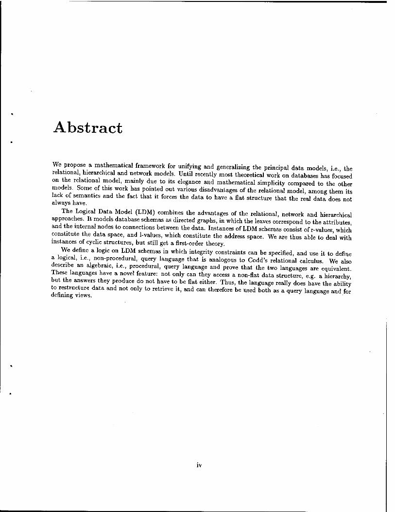
Example 4: In practice we would probably not use the hierarchy of Fig. 5 as a representation of the genealogy, since it contains a lot of duplicated information. If a person appears in the database as both a child and as a parent, he will appear in both the Person and Parent records. For this reason, we would probably use a hierarchy with virtual records, as shown in Fig. 7. The corresponding LDM schema is then the cyclic schema in Fig. 8.
If the contents of the database are the same as before, the corresponding instance of the LDM schema is
I(u) = {Rehoboam, Solomon, David, Batsheba, Jesse}
I(v) = {(Jesse, 0),
(David, {(Jesse, 0)}),
(Batsheba, 0),
(Solomon, {(David, {(Jesse, 0)}), (Batsheba, 0)}),
(Rehoboam, {(Solomon, {(David, {(Jesse, 0)}), (Batsheba, 0)})})} I(w) = {0, {(Jesse, 0)}),
{(David, {(Jesse, 0)}), (Batsheba, 0)},
{(Solomon, {(David, {(Jesse, 0)}), (Batsheba, 0)})})}
3.1.4. Instances of LDM Schemas
As we see in Example 4, when the schema is cyclic and the nesting depth is large an instance can be rather complicated. If the data as well as the schema was cyclic, then the nesting depth would be infinite and we would not be able to write the instance down at all. This is similar to one of the problems with Jacobs'
10 CHAPTER 3. INTRODUCTION TO THE LOGICAL DATA MODEL
Person
Virtual Person
Figure 7: The genealogy as a hierarchy with virtual records
Figure 8: LDM schema corresponding to Fig. 7
database logic. The mathematical theory we develop to deal with this problem is closely related to the non well-founded sets of [Acz85]. Our approach to defining an instance of a schema is to model abstractly the concept of memory addresses and their contents. We use the term "1-values" for the abstract memory addresses, and the term "r-values" for their contents. An instance I then consists of two parts
1. An assignment of a set 7(w) of 1-values (abstract addresses) to each node u of the schema.
2. An assignment of an r-value r(l) to each 1-value / in /(«).
These 1-values are taken from a fixed set L which will usually be the set of natural numbers. We now show what some of the instances in the previous examples look like when we use 1-values and r-values.
Example 5: The instance of the schema in Example 1 consists of the following assignment of 1-values to nodes.
I(u) = {1,2,3}
I(v) = {4,5,6,7}
and
I(w) = {8,9,10,11}
We then assign an r-value r(l) to each of these 1-values. This assignment is shown in Fig. 9.
Example 6: In Fig. 10 we show the instance using 1-values and r-values that corresponds to the instance of Example 4. Fig. 11 shows the links between the 1-values and their r-values pictorially.
3.1.5. The Entity-Relationship Model
We conclude this section by showing how the logical data model can also be used to describe data structured by the Entity-Relationship Model of [Che76].
To map an entity-relationship schema into an LDM schema, we represent each entity type as a D- node, and each relationship record as a O-node. A 1-1 arc from a relationship record to an entity type is represented by an edge from the corresponding O-node to the corresponding D-node, while for a many to

3.2. QUERY LANGUAGES 11
/ r(0 1 2 3
Rehoboam Solomon
David
r(l)
Solomon David
Batsheba Jesse
I(w)
I r(Z)
8 (1,4) 9 (2,5)
10 (2,6) 11 (3,7)
Figure 9: Instance of the LDM schema that corresponds to a relation
I(u)
/ r(0 1 Rehoboam 2 Solomon 3 David 4 Batsheba 5 Jesse
I(v) I(w)
I r(l)
6 (1,H) 7 (2,12) 8 (3,13) 9 (4,14) 10 (5,14)
/ r(l)
11 {7} 12 {8,9} 13 {10} 14 0
Figure 10: Instance of the LDM schema that corresponds to a hierarchy
one arc the connection is through a O-node. Figures 12 and 13 show two examples of entity-relationship database Schemas from [Che76], together with the corresponding LDM Schemas.
3.2. Query Languages
In this section, we give some examples of logical and algebraic queries on LDM Schemas. All these examples are of queries that we can write in the query languages that we shall describe later on. The languages we describe later, however, are more formal, and therefore harder to use. The analogous situation in the relational model, is the comparison between Codd's tuple calculus and languages like QUEL. The languages in the current section have not been fully developed, and we describe them mainly as motivation for the formal presentation in the following chapters. In all the examples in this section, the database schema will be the LDM representation of the hierarchy, i.e., the schema in Fig. 14, together with the instance in Fig. 15.
3.2.1. The Logical Query Language
Both the logical and algebraic query languages have the property that the result can have a more general structure than a relation—in fact it is structured according to some LDM schema that is specified as part of the query. A query consists therefore of a specification of the nodes of the query, together with some QUEL-like statements specifying the contents of these nodes.

12 CHAPTER 3. INTRODUCTION TO THE LOGICAL DATA MODEL
• 11
\ \
e : i
/ 1
Rehoboam
w
Figure 11: Pictorial representation of the instance in Fig. 10
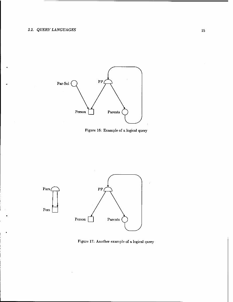
Example 7: Our first query adds a new node Par-Sol of type O with child Person (see Fig. 16). This node contains the set of parents of "Solomon." The query is
type of Par-Sol is (collect,Person) range oi t is PP range oi u is PP retrieve S into Par-Sol where S={u. Person} and t.Person="Solomon" and u is in t.Parents.
Example 8: In this example, we show how to restructure the database in the form shown in the left part of Fig. 17. We first copy all the people in the node Person into the node Pers
type oi Pers is basic range oi t is PP retrieve t.Person into Pers
The node Pars then contains all pairs that correspond to Person-Parent pairs.
type oi Pars is (composition,Pers,Pers) range oi t is PP range oi u is PP retrieve (t.Person,u.Person) into Pars where u is in t.Parents.
3.2.2. The Algebraic Query Language
Example 9: We show how we could compute the query of Example 7 by a sequence of algebraic operations.

3.2. QUERY LANGUAGES 13
Department
Dept-Emp
N
Employee
Department
Employee
Figure 12: Department-Employee example
1. Select those elements of PP whose first component is "Solomon," i.e., *i = <rCperson=«s l »l(PP) (Fig. 18).
2. Do another type of selection: Select those sets that actually appear in tuples in ti. This is the operation
*2 = ^Parents in(*0 (FiS- 19)- 3. We now have almost what we want, the only difference being that t2 contains elements of PP rather
than of Person. We have to do a dereferencing step, i.e., project onto Person. The operation is *3 = Hpersonte) (Fig. 20).
The entire query is therefore
nPerson°'Parentsin0'(Person="Solomon")(PP)

14 CHAPTER 3. INTRODUCTION TO THE LOGICAL DATA MODEL
Employee Prqj-Worker
o
Project
Employee Project
Figure 13: Project-Worker example
Person
Figure 14: LDM Schema
J( Person) J(PP)
I r(0 1 Rehoboam 2 Solomon 3 David 4 Batsheba 5 Jesse
/ r(l)
6 (1,11) 7 (2,12) 8 (3,13) 9 (4,14) 10 (5,14)
J(Parents)
/ r(Z)
11 {7} 12 {8,9} 13 {10} 14 0
Figure 15: Instance of Fig. 14
3.2. QUERY LANGUAGES 15
Par-Sol
Person
Figure 16: Example of a logical query
ParsQ
Pers : :
Person
Figure 17: Another example of a logical query

16 CHAPTER 3. INTRODUCTION TO THE LOGICAL DATA MODEL
1(h)
I r(l)
15 (2,12)
*iQ
Person
Figure 18: First step of the algebraic query
I(t2)
I r(/) 16 {8,9}
Person
Figure 19: Second step of the algebraic query

3.2. QUERY LANGUAGES 17
I(t3)
I r(l)
17 {3,4}
Person
Figure 20: Third step of the algebraic query
Chapter 4
LDM Schemas and Instances
In this chapter we start the formal description of the logical data model. We define the two basic components of the model: LDM Schemas, that describe how data is structured, and instances of these Schemas.
4.1. LDM Schemas
The definition of a schema is essentially the same as outlined in the previous chapter. We have to go into several technical details that were not mentioned there. If v is a node of type O, its domain consists of tuples formed from its children. For this to be meaningful we need an order on these children. Since there may be more than one edge between v and a node w, we also need an order on the occurrences of w in these tuples, so that what we really need is an order on all the edges with tail v. For simplicity, instead of using one order per node v we shall use a total order on all the edges of the schema.
Another technical detail is that a schema includes a set of constants. The reason for this is that we want to have a precise analogy between schemas and instances, on the one hand, and logical theories and models, on the other. The set of constants plays the role of individual constants in a logical theory.
Definition 1: A schema, is a tuple S = (V, E, <, p, C) where:
1. (V, E) is a directed multigraph.
2. < is a total order on E.
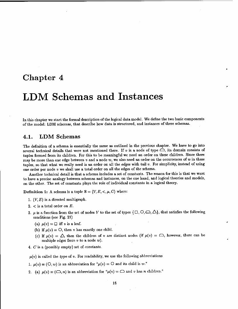
3. ß is a function from the set of nodes V to the set of types { D, O, O, A}, that satisfies the following conditions (see Fig. 21)
(a) fi(v) = D iff v is a leaf.
(b) If fi(v) = O, then v has exactly one child.
(c) If /J,(V) = A then the children of v are distinct nodes (if n(v) = Q, however, there can be multiple edges from v to a node w).
4. C is a (possibly empty) set of constants.
p(v) is called the type of v. For readability, we use the following abbreviations
1. ß(v) = (O, w) is an abbreviation for up(v) = O and its child is w."
2. (a) n(v) = (O, n) is an abbreviation for "/J,(V) = O and v has n children."
18

4.2. INSTANCES OF LDM SCHEMAS 19
D r^ Q
Figure 21: Nodes in LDM Schemas
(b) p(v) = (O, n, vi,..., vn) is an abbreviation for up(v) = O, there are exactly n edges ex, ..., e„ with tail v, these edges are in the order ei < • • • < e„ and their heads are vi, ..., i>„."
3. (a) ß(v) = (A, n) is an abbreviation for "//(v) = A and v has n children."
(b) p(v) = (A, n,vi,..., vn) is an abbreviation for "n(v) = /S, there are exactly n edges d, ..., e„ with tail v, these edges are in the order ei < • • • < e„ and their heads are «i, ..., vn."
Some other abbreviations that we shall use include referring to elements of V and E as nodes and edges, respectively, of S, and referring to < as an order on the children of a node of S. We shall ignore the order < when it is clear from the context, and we shall often refer to a schema as (V, E, /*, C).
As we outlined in the previous chapter, one part of a query on an LDM schema S is the addition of some nodes to S. We formalize this as follows
Definition 2: Let S = (V, E,<,fi, C) be a schema. S' = {V, E', <', //', C) is an extens/on of S iff
1. VCV
2. (a) E C E'
(b) If (vi,v2) £ E' - E then vi is in V, i.e. all new edges are either between new nodes, or from a new node to a node in V.
3- <'|jExJS=<
4. (j! \V= p
4.2. Instances of LDM Schemas
Throughout this section S = (V, E, ß, C) will be a fixed LDM schema. An instance of S consists of two parts: An assignment of a set of objects called I-values to each node of S, and an assignment of an object called its r-vaiue to each such 1-value.
In the format model instances are constructed recursively from the leaves up. Since our model allows cycles, we cannot use this approach. What we do instead is define when a given object I is an instance.
Definition 3: An instance of S is a tuple I = (/, r, f) that satisfies:
1. / is a function with domain V. This is the assignment of sets of 1-values to nodes. We require that I(v) and I(w) be disjoint whenever v and w are distinct nodes of S.
2. r is a mapping with domain Uv€VI(v), i.e., from the set of all the 1-values that are in the instance. The mapping r must satisfy:

20 CHAPTER 4. LDM SCHEMAS AND INSTANCES
(a) If n(v) = (0,n,i>i, ...,«„) and / € I(v), then r(l) is a tuple (h, ...,/„) such that for each i, 1 < i < n, U is an element of I(vi).
(b) If IJ,(V) = (O, w) and / € I(u), then r(f) is a subset of I(w).
(c) If ß(v) = (A n, »l, • • •, «n) and / G J(t>), then r(/) G J(»i) U • • • U /(«„).
Note that in general there is no constraint on the range of r on nodes of type D.
3. / is a function with domain C. For each c G C, f(c) is the interpretation of the constant c. In general there is no constraint on the range of /.
If I is in U„ev*(«)> we say that ü is an ^vaiue in *> and r(0 is called its r"vaJue- The set Uoev»*[/(w)] is called the set of r-values in I.
Definition 4: A finite instance of S is an instance I = (7, r, /) of S such that for each node v of S, I(v) is
finite.
In practice, except for the reduction to first-order logic in Sections 5.2 and 5.3, we shall only be interested in a restricted class of instances, those that correspond to real databases. Such an instance is finite, and the instance I(v) of each node v is a set of natural numbers. For a given database schema, there is also a fixed set D from which the data is taken. If v is of type D and Z G I(v), r(l) must belong to the set D. Furthermore, each constant c G C must also belong to D, and we do not distinguish between c and /(c). In short, after Section 5.3 we shall talk about Schemas (V,E,fj) and instances (I,r), where all the 1-values are natural numbers, and all the data and constants are taken from a fixed set D.
Definition 5: Let I be an instance of the schema S, and let v be a node of S of type (Q, n, vx,..., v„). Let / be any 1-value in I(v). If 1 < i < n, then IL(Z) will be the ith component of r(l). We shall also use the notation !!„;(/) for this component, whenever this does not result in any ambiguity.
The following definition is related to when we can compare two 1-values, i.e., if v and w are nodes of S, h G I(v) and l2 G I(w), is it possible for h and l2 to have the same r-value?
Definition 6: We say that two nodes v and w in a schema S are similar iff they are of the same type and have the same children, i.e., if one of the following holds:
1. n(v) = IJ,(W) = D.
2. For some node u, n(v) = n(w) = (0,u).
3. For some n and nodes ui,...,u„, n(v) = n(w) = (Q,n,ui,.. .,««)•
4. For some n and nodes ui,..., u„, fi(v) = p(w) = (A n, ui,..., un).
We would like to be able to show that whenever r(h) = r(/2) for some h G I(v) and l2 G I(w), then v and w must be similar. However, this may not be true for v or tu of type D. For example if fi{v) = D, since there is no constraint on the range of the function r on I(v), the r-value of h may just happen to have the form of a tuple or set of 1-values. The logic will be defined in such a way that we shall only be able to compare r-values of similar nodes, so that this will not cause any problems.
Let S' be an extension of S. We define an extension of I to an instance of S' as follows.
Definition 7: Let S' be an extension of S, and let I = (I, r, f) be an instance of S. We say that an instance I' = (/', r', f) of S' is an extension of I to S' iff
1. For all v in V, I'(v) - I(v).
4.2. INSTANCES OF LDM SCHEMAS 21
2. If v is a node of S and / € I(v), then r'(l) = r(/).
The proof of the following lemma is straightforward.
Lemma 1: Let S' be an extension of S, and let I' be an instance of S'. Then there is a unique instance I of S such that I' is the extension of I to S'. This instance is called the restriction of I' to S. |
We conclude this chapter with a definition of isomorphism. Two instances will be isomorphic if they are essentially the same, i.e., if they differ only by renaming of 1-values. As we shall want to show that the result of a query is well-defined up to isomorphism, we give a stronger definition of isomorphism. Let I be an instance of S, let S' be an extension of S and let Ix and I2 be extensions of I to S'. We shall say that Ii and I2 are isomorphic relative to S, if there is an isomorphism between Ii and I2 that leaves the elements of I fixed. In the case of a query, this will mean that an isomorphism relative to the database leaves the contents of the database fixed.
Definition 8: Let S' be an extension of S and let I = (I,r,f) be an instance of S. Let Ii = (h,ri) and h = (h, r2) be two extensions of I to S'. We say that Ii and I2 are isomorphic relative to S iff there is a mapping
such that
1. For each node v of S', g maps I\(v) onto h(v).
2. For each node v of S, g is the identity on I(v).
3. If v is a node of S' and / G h(v), then
(a) If v is of type D, then r2(g(l)) = ri(l).
(b) If v is of type (O, n), then
r2(</(0) = Un!^/))),...,,^^))!
(c) If v is of type /S, then r2(g{l)) = g(ri(l)).
(d) If v is of type O, then g[r2(l)) = rx[</(/)].
As a special case of this definition we get the definition of ordinary isomorphism.
Definition 9: Let Ii = (h,ri) and I2 = (I2,r2) be instances of S. We say that Ix and I2 are isomorphic iff they are isomorphic relative to the empty schema, i.e., the schema with V = E = ß = 0.

Chapter 5
The LDM Logic
5.1. Definition of the Logic
In this chapter we define the LDM logic. Our goal is to define a logic that is similar to the relational tuple calculus. We then use this logic as part of the logical query language. As the logic will resemble the relational tuple calculus, we can also use it to specify integrity constraints on LDM Schemas, and to define views.
Throughout this chapter S = (V, E, p, C) will be a fixed schema, and I = (7, r, /) will be a fixed instance of S, unless mentioned otherwise. Each variable in the LDM logic has a fixed sort, where the sorts are the elements of V. The sorts restrict the possible values that the variable may have. For example, if a; is a variable of sort v then x can take only values in I(v). The analogue to this in the relational calculus is a tuple variable that ranges over a specific relation. We shall usually write a variable with its sort as a subscript, e.g., xv. Two variables with different subscripts will denote distinct variables, so that xu will be a different variable from xv. Even though variables range over 1-values, we shall often say "the 1-value of xv" instead of "the value of xv," and "the r-value of xv" when what we really mean is "the r-value of the value of*„."
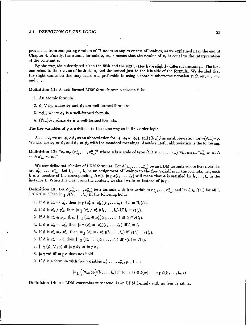
Definition 10: The atomic formulas over S are the following:
1. xv ivt yw, where w is a node of type Q and v is its 2th child.
2. xv pyw, where to is a node of type A.and v is one of its children.
3. xv £yw, where w is of type (0,v).
4. xv =; yv ■
5. xv =r yw, where v and w are similar nodes.
6. xv =r c, where c is an element of C, and v is of type D.
The atomic formula xv %t Vw means that the 1-value of xv is the 2th component of the r-value of yw. Note that we have to mention which component of w we are referring to, since there may be multiple edges from w to v. However, we shall also write xv irv yw when this is unambiguous. xv p yw means that the r-value of yw is xv. Since there are is only one edge from w to v, we use p rather than pt. xv € yw means that xv is a member of the r-value of yw.
There are several different kinds of equality. xv =; yv means that the 1-values of xv and yv are equal. Since I(v) and I(w) are disjoint whenever v ^ w, the logic has no atomic formula of the form xv =/ yw
for v ^ w. xv =r yw means that the r-values of xv and yw are equal. We restrict this to similar nodes to
22
5.1. DEFINITION OF THE LOGIC 23
prevent us from comparing r-values of D-nodes to tuples or sets of 1-values, as we explained near the end of Chapter 4. Finally, the atomic formula x„ =r c means that the r-value of xv is equal to the interpretation of the constant c.
By the way, the subscripted r's in the fifth and the sixth cases have slightly different meanings. The first one refers to the r-value of both sides, and the second just to the left side of the formula. We decided that the slight confusion this may cause was preferable to using a more cumbersome notation such as /=;, r=r
and r=/.
Definition 11: A well-formed LDM formula over a schema S is:
1. An atomic formula
2. 4>i V 4>2, where <f>i and 4>2 are well-formed formulas.
3. -i^i, where </>i is a well-formed formula.
4. (Vxv)4>i, where <j>\ is a well-formed formula.
The free variables of <f> are defined in the same way as in first-order logic.
As usual, we use 4>\f\<f>2 as an abbreviation for ->(-><f>i V-xfo), and (3xv)<f> as an abbreviation for ->(Vx„)-^. We also use 4>i => <f>2 and ^i •» fa with the standard meanings. Another useful abbreviation is the following.
Definition 12: "xv =r (x^,..., x£j" where v is a node of type (O, n,vlt...,vn) will mean "sj, xi xv A ■■■Ax1n x„ xv."
We now define satisfaction of LDM formulas. Let ^(x^,..., x£J be an LDM formula whose free variables are x^, ..., x£n. Let lt, ..., /„ be an assignment of 1-values to the free variables in the formula, i.e., each /, is a member of the corresponding I(vi). |= j <j>(li ,...,/„) will mean that 4> is satisfied by lx ,...,/„ in the instance I. When I is clear from the context, we shall write (= instead of \= j .
Definition 13: Let ^(x^,..., x£J be a formula with free variables xjt,..., x£ , and let /, € I(vi) for all i, l<i<n. Then |= j <0(/i ,...,/„) iff the following hold:
1. If <}> is 4 xt yl, then ^j (xj, xt x>w)(lu .. .,/„) iff/, = Ht(lj).
2. If <f> is 4 p yl, then h I K P <)(h, ...,/„) iff fc = r(lj).
3. If <f> is x[ € xl, then (=1 (4 G *l)(h, • •-,/„) iff /< € r(/,-).
4. If ^ is xj, =, x>, then 1=! (xj, =, xl)(llt.. .,/„) iff/; = /,.
5. If <j> is x{, =r xi, then \=j (xj =r xi){h,. ..,/„) iff r(h) = r(lj).
6. If <t> is xj, =r c, then 1=! (xj, =r c)(lu. ..,/„) iff r(h) = f(c). 7- hi (4>i vfa) iff l=i <^i or hi fa- 8. |= j ~«f> iff |= j <j> does not hold.
9. If 4> is a formula with free variables xj ,..., x" , 2/„,, then
1=1 ((Vy„)*)(Ji,.. .,/„) iff for all / € /(«/), (=! M,. ..,/„,/)
Definition 14: An LDM constraint or sentence is an LDM formula with no free variables.

24 CHAPTER 5. THE LDM LOGIC
Definition 15: A constrained schema is a pair (S, <j>), where S is a schema and <f> is an LDM constraint over S. An instance of (S, <j>) is an instance I of S that satisfies (= j <j>.
Definition 16: Let <f> be an LDM sentence. We say that an instance I of S satisfies <j> iff |=j <f> holds.
Definition 17: Let E be a set of LDM sentences, and let <j> be an LDM sentence. We say that £ (=<£ iff for every instance I of S that satisfies all the sentences in S, hi ^ holds.
Definition 18: Let 4> be an LDM sentence, and let <f> be an LDM sentence. We say that <p is valid iff for any instance I of S, \= j <f> holds.
Example 10: This example and the next one will be over the LDM schema of Fig. 8 (page 10) with the instance of Fig. 10 (page 11). The LDM formula <l>(xu, yv) = (xu xi yv) says that the 1-value of xu is equal to the first component of the r-value of yv. f=I <f>(h,h) holds for the (h,l2) pairs (1,7), (2,8), (3,9), (4,10),
and (5,11).
Example 11: Let us see how to write a constraint that says that each 1-value of u is related to exactly one set in w. So for example, '8' and '9' as parents of '2' must be in one set rather that in two different sets. The constraint is
4> = (Vxu)(Vyi)(Vy„2)(V4)(V4) (vl =r (*«, 4) A yl =r (*«, 4) => 4 =» 4J
In other words, each 1-value in u (xu) has at most one 1-value in w (4 and z£) associated with it. This association is through yj and y$.
Note that this constraint says that each i-value in u is associated with at most one set in w, rather than saying that each person in the database is associated with at most one such set. There could still be duplication in u, e.g., two 1-values with the r-value "Solomon." One way to prevent this would be through the constraint
V> = (Vxi)(V*»)(*i =r *l => *i =/ *«)
The following lemma shows that we can restrict the logic without reducing its power. We show that there is no need for atomic formulas that compare r-values of internal nodes. This lemma will make some subsequent proofs and definitions much simpler.
Lemma 2: Let ^(z^,.. .,<„) be an LDM formula whose free variables are the variables x^, ..., <„. There is an LDM formula ^(ijj, • • •,<„) with the same free variables, that does not contain any atomic subformula of the form xu =r yv with n(v), n{w) ^ D. This formula is equivalent to <f>, i.e., for all instances
TofSandall/i, ...,/„, h €/(«<), hi M. •••>'») iff Nl tf(*i.-■■.*»)•
Proof: The proof is by induction on the size of <j>. We show how to construct ip for formulas of the form xu =r yv, where u and v are similar and not of type D. The result will then follow immediately.
We distinguish between the possible types of v and w.
1. If u and v are of type (0,tu), then i/>(xu,yv) will be (VzU))(zul € xu «• zw G yv), where zw is some new variable. Let I be an instance of S. Then
hi (*«. =r Vv)(k,h) *> r(h) = r(l2) & For all / in I(w), I G r(h) & I G r(/2)
«•hi ((V«U))(z«> € xu « zw G yv)){hM)
and therefore <j> <£■ tp is valid.

5.1. DEFINITION OF THE LOGIC 25
2. If u and v are of type (O, n, wu ..., wn), then ip(xu, yv) will be
(V4i) • • • (V«S.) ((4, »l *«'<*• 4, »l 0») A • ■ • A (z£n x„ zu 4* *Sm *» ».))
where 4^ •••» *£„ are n different new variables. Let I be an instance of S. Then (=j (;c„ =r y„)(/i,/2) is equivalent to r(h) = r(/2). If r(/i) = (/},..., /?) and r(/2) = (/*,..., J»), r(/i) = r(/2) is equivalent to /][ = /2, for i = 1, ..., n. In other words, for each such i,
hi f (V4)(4,- «•< *« <*•4,- »t ib)J(ii><3)
and therefore (= j (zu =r j/„)(/i,/2) is equivalent to
hi (v4,)• • •(VzS„)((41 ""l *« *> 4, TI y«)
A • • • A (z£n *7> »u <*• 2S„ *n Vvj) (h, h)
i.e., <f> o- ^ is valid.
3. If u and « are of type (A », ™i, ■ ■ •, wn), then i>(xu,yv) will be
(341)(41P*«A41p|fe)V---V(3«2J(a2mpa!t,AaSwpife)
where z^, ..., Z£B are n different new variables. Let I be an instance of S. Then |=j (a;u =r yv)(h,h) is equivalent to r(/i) = r(/2) = /. This can hold only if for some i, 1 < i < n, I 6 !(«><) in which case
hI ((3*1,)«, P *« A 4; /> yv)) (h, h)
and therefore (f> & V is again valid. |
From now on, we shall assume that xu =r yv can appear as a subformula only when (i(v) = fj,(w) = D, as far as proofs and definitions are concerned. We shall continue to use the more general form when convenient.
The proof of the following lemma, that says that satisfaction is preserved under isomorphism, is straight- forward.
Lemma 3: Let S' be an extension of S, and let Ii and I2 be extensions of I to S'. Let g be an isomorphism from Ii to I2 relative to S, and let <j>(xlVi,..., x^j be an LDM formula. Then
\=I1'Kh,...,ln)o\=i34(g(li),...,g(ln)) I
Lemma 4: Let ^(x^,..., x%J be an LDM formula over S whose free variables are xllt...,x^. Let I be a finite instance and let U € I(vt) for all i, I < i < n. Then \=i<j>(llt. ..,/„) can be determined effectively.
Proof: We show this by induction on the size of the formula. For atomic formulas testing for satisfaction is straightforward. Testing for disjunction and negation is also clearly effective. For quantification we make use of the finiteness of I. In order to test whether \=j ((Vy„,)<£)(/i, ...,/„), we test whether \=j<f>(h, ...,/„,/) for each / in the finite set I(w). |

26 CHAPTER 5. THE LDM LOGIC
5.2. The Relation between LDM logic and First-Order Logic
In this section we shall show that the LDM logic is essentially first-order; that is, it is compact and it satisfies a Löwenheim-Skolem theorem. We shall prove this by reducing LDM logic to a certain many-sorted first- order logical theory with equality. We mention in contrast that Jacobs' database logic [Jac82] is inherently a higher-order logic that does not have any of these properties. In the next section, we shall use this reduction to develop a proof theory for the LDM-logic. In both these sections we shall not assume that instances are finite, or make any of the other assumptions on instances that we mentioned earlier.
Let L be an LDM logic over S. We construct a many-sorted first order logic with equality V as follows. The sorts of L' are V U {c}, i.e., we have a sort v for each node of the schema, and one special sort c that corresponds to the domain from which the data is taken. V has variables ranging over all the sorts, except for the special sort, c since we do not want to be able to quantify over the data domain.
The relation symbols of L' are
{€«,| w G V and p,{w) = O} U {pw,v \ w G V, fi(w) = A and v is a child of w}
If w G V is of type (O, v) then G«, is a binary relation symbol between elements of sorts v and w. pw>v is also a binary relation between these sorts. We shall use infix notation for binary relations.
The function symbols of L' are
{*«,« | tu G V,it(w) = (0,n), 1 < i < n] U {/„ | w G V,fi(w) = D}
The function symbol TWii is from sort w to sort v, where v is the ith child of to. We shall also use the notation TWIV when its meaning is unambiguous. The function symbol /„, is from sort w to sort c. Intuitively, x«,^ maps its argument to its ith component, and /„, maps its argument to its r-value, which is a data element. The reason we use pw>v, rather than a function symbol, is that p should be interpretated as a function from I(w) to the union of the instances of its children, whereas in first-order logic all functions are to exactly one sort. For this reason we use a relation symbol for p, and we shall also need some extra axioms for L' besides the usual logical axioms. Finally, the constants of L (i.e., the elements of C) are also constants of L', of sort c.
The logical theory L' then consists of the standard logical axioms, together with the set Ax(S) of axioms for p. Ax(S) contains the following axioms for each node w of S that is of type (/S, n, v\,..., vn).
1. (Va^ayJJfoJ, pw,Vl xw) V • • • V (BtfJGff. *».•- *"))
2. For all i and j where 1 < i,j < n and i ^ j, (^xw)^(3yi.)(y'v. pw,Vi xw) => (Vyji)-i(yj;. pw,Vixw))
3. For all», 1 < i < n, (V*«,)^.)^,)^. pw,Vi *«,) A (j^ pw<Vi xw) => (yj, =, y%.))
Essentially these axioms say that the interpretation of p is a function from I(w) to J(ui)U • • -Lll(vn). When we use the symbol }= in the theory L', e.g., E \=<f>, we shall mean that every model of E and Ax(S) is also a model of 4>.
We now define two mappings. The first, F (for "First-order") will map formulas and instances of the LDM logic L to formulas and structures of L'. The second mapping, L (for "LDM") will map L' to L.
5.2.1. Mapping LDM Logic into First-Order Logic
We first show how to map LDM formulas into first-order formulas.
5.2. THE RELATION BETWEEN LDM LOGIC AND FIRST-ORDER LOGIC 27
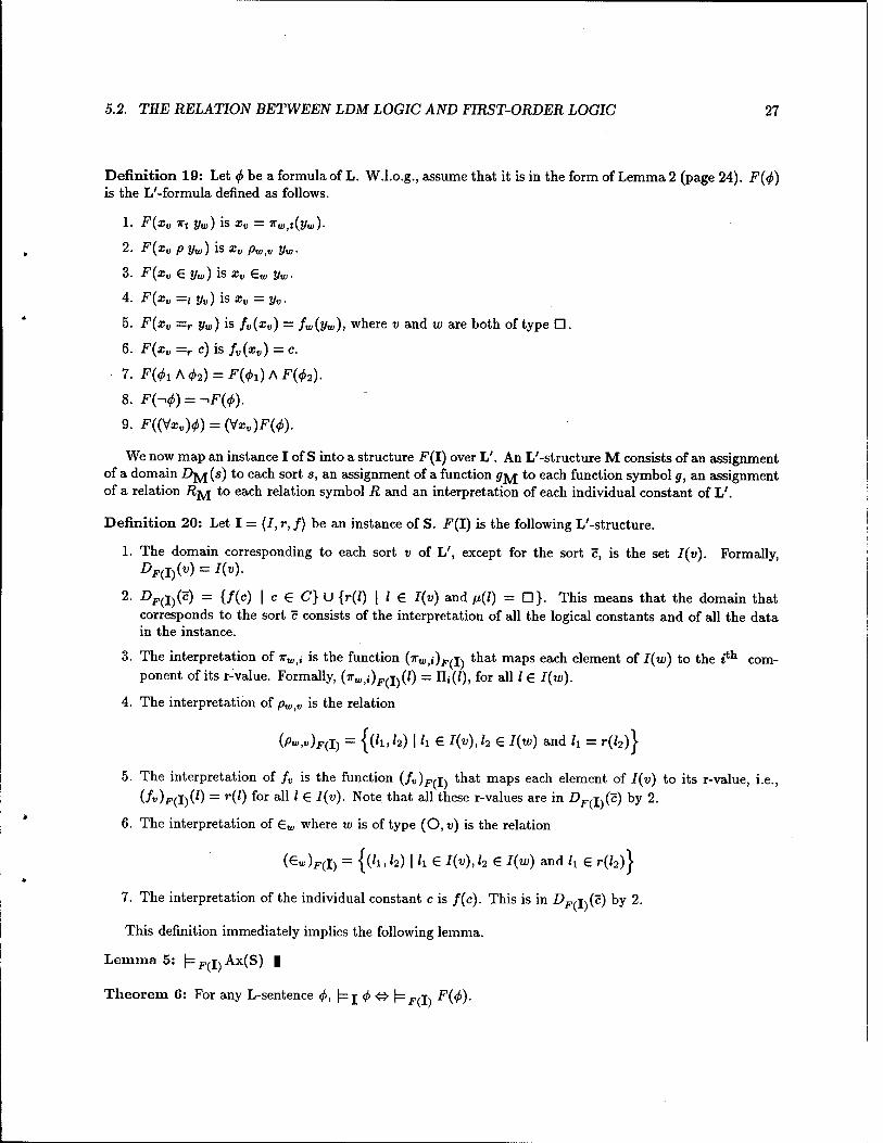
Definition 19: Let <j> be a formula of L. W.l.o.g., assume that it is in the form of Lemma 2 (page 24). F(<f>) is the L'-formula denned as follows.
1. F(xv xt yw) is xv = TTWtt(yw)-
2. F(xv pyw) \sxv pWtV yw.
3. F(xv e yw) is xv G«, yw.
4. F(xv =j yv) is xv=yv.
5. .F(:c„ =r yw) is fv(xv) = fw(yw), where t; and u; are both of type D.
6. -F(a;„ =r c) is /„(a;,,) = c.
7. F(<t>1A<j>2) = F(<f>1)AF(4>2).
8. F(-.^) = -iF(tf).
9. F((V^)^) = (Vxv)F(<f>).
We now map an instance I of S into a structure F(I) over L'. An L'-structure M consists of an assignment of a domain DJ^J (s) to each sort s, an assignment of a function </j^ to each function symbol g, an assignment of a relation ÄJ^J to each relation symbol R and an interpretation of each individual constant of L'.
Definition 20: Let I = (I, r, f) be an instance of S. .F(I) is the following L'-structure.
1. The domain corresponding to each sort v of L', except for the sort c, is the set 7(w). Formally,
2. Djp(i)(c) = {/(c) | c G C} U {r(/) | / € I(v) and ß(l) = D}. This means that the domain that corresponds to the sort c consists of the interpretation of all the logical constants and of all the data in the instance.
3. The interpretation of TWii is the function (Trw,i)F,i) that maps each element of I(w) to the ith com- ponent of its r-value. Formally, (?Tt»,i)jsvi)(0 = IL(/), for all / G I{w).
4. The interpretation of pw>v is the relation
(/V»)f(I) = {(h,h) | h G I(v),l2 e I(w) and h = r(/2)}
5. The interpretation of /„ is the function (/«)f(i) that maps each element of I(v) to its r-value, i.e., (/«)F(I)(0 = r(0 for all I G I(v). Note that all these r-values are in DprfJc) by 2.
6. The interpretation of G«, where w is of type (O, v) is the relation
(€»)F(I) = {(h,h) | h G /(»), h G J(t») and /x G r(/2)}
7. The interpretation of the individual constant c is /(c). This is in DF(iJc) by 2.
This definition immediately implies the following lemma.
Lemma 5: \= f,j\ Ax(S) |
Theorem 6: For any L-sentence <f>, \= j <f> <t> \= F(i) F(4>).
28 CHAPTERS. THE LDM LOGIC
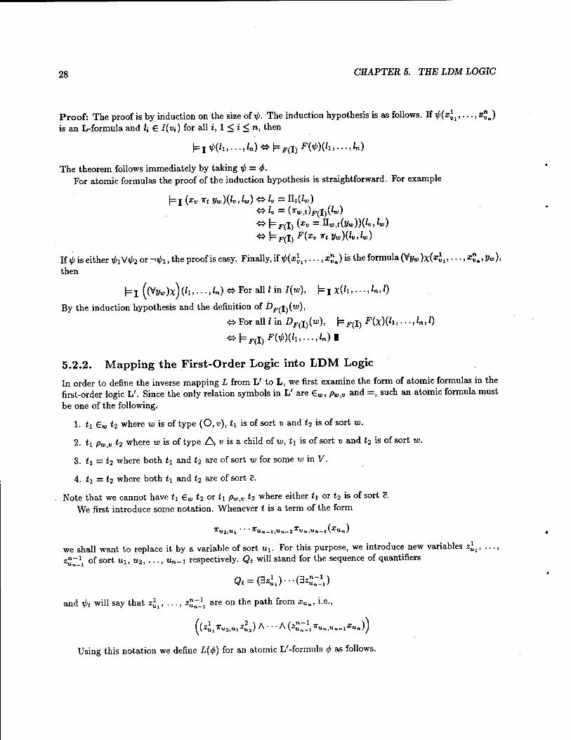
Proof: The proof is by induction on the size of ip. The induction hypothesis is as follows. If ^(«J, ,-••,*?„) is an L-formula and U € I(vi) for all i, 1 < i < n, then
Ni*('i WoNfuWK'i W
The theorem follows immediately by taking ^ = <f>- For atomic formulas the proof of the induction hypothesis is straightforward. For example
** N F(I) (*» = nt»,*(y«;))(^> *«>) <*(= r(i) ^(s« *t y<«)('«, it«)
If V is either V>i Vi/>2 or --Vi. the proof is easy. Finally, if t/'OcJ,, • • •, <„) is the formula (Vyu,)x(41. • • • > <„> V«>)> then
t=l((Vyu,)x)0i,- ..,/„)^For all/ in /(to), |=I xtfi,---.*».*)
By the induction hypothesis and the definition of i>F(j^{w),
& For all / in £>F(I)(to), (= F(J) F(x)( *i ^ 0
5.2.2. Mapping the First-Order Logic into LDM Logic
In order to define the inverse mapping / from L' to L, we first examine the form of atomic formulas in the first-order logic L'. Since the only relation symbols in L' are 6«,, />«,,« ^ => such an atomic formula must be one of the following.
1. h Ew t2 where w is of type (O, v), ti is of sort v and t2 is of sort to.
2. ti pw,v t2 where to is of type A " is a child of to, ix is of sort v and f2 is of sort w.
3. ti = <2 where both ti and i2 are of sort to for some to in V.
4. <i = t2 where both 11 and <2 are of sort c.
Note that we cannot have U Ew t2 or h pw>v t2 where either ti or t2 is of sort c. We first introduce some notation. Whenever t is a term of the form
XU2,Ul - ' •"'o„_l,Un_3XUn,«n-l(:E«n)
we shall want to replace it by a variable of sort «i. For this purpose, we introduce new variables z\v ..., z%~* of sort ui, u2, ..., «n-i respectively. Qt will stand for the sequence of quantifiers
Qt = (3zi1)---(3z^1)
and V< will say that zxUl, ..., z^~\ are on the path from xUn, i.e.,
((«ix»«».«!*^) A • • • A (Cl'«..«.-!'».))
Using this notation we define /(<£) for an atomic L'-formula <f> as follows.

5.2. THE RELATION BETWEEN LDM LOGIC AND FIRST-ORDER LOGIC 29
1. Since the result of each /„ is of sort c and there are no function symbols from sort c, whenever </> is ti Gui h or t\ pW)V t2, the only possible form that the terms t\ and t2 can have is
h = i"«i,tiTu3,ui • • •"«„,«„_!?[■«,«„(£«)
and
(n or m may be equal to 0, in which case some of the new variables are not needed. It should be obvious how to modify the definitions in this case, and in the case when tx or t2 is an individual constant.) We now define
L{h €w h) = QtlQt3 (ipu A ipta A (z„ 6 zw)\
where z„ and zw are the new variables of sorts v and w that we introduced.
In a similar way L(ty pWiV t2) is defined as as
QnQt, (v»*! A i/)ta A (zv p zwy)
2. When <j> is 11 = t2 where tx and t2 are of sort w, ti and t2 must be of the form
t\ = Tuj.tuTua,«! • • •Tun,o„_i1'u,ti„(*u)
and
h = T»I,UI*„;,,„! •••i"«m,«m_1T«,t.„(y«)
We then define L(t1=t2) = QtlQta(rj}tlAi>t3A(zl=,zl))
where z£, and z£ are the two new variables of sort w that we introduced.
3. When <j> is tx = t2 where tx and t2 are of sort c, tx and f2 must have the form
<i = /»Juj,»! • • •TUn|U„_1TU|Un(aju)
and
Write <! = /Ul(i3) and i2 = fVl(U)- We then define L(h = t2) to be
Qt3QU (it, A Vt4 A « =r <))
Definition 21: When <£ is an L'-formula, L{4>) is defined as follows.
1. If <j> is an atomic formula L{<f) is defined above.
2. I(^iA^) = L(^)ALW.
3. £(-.0) = -.i(^).
4. L((Vxv)<f>) — (Vxv)L(4>). The fact that L' has no variables of sort c is necessary to guarantee that this is an L-formula.
We now show how to map L'-structures into L-instances.
30 CHAPTER 5. THE LDM LOGIC
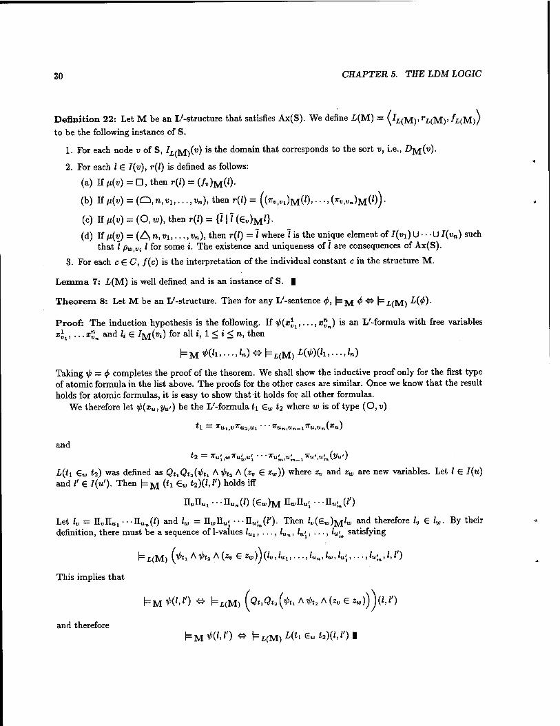
Definition 22: Let M be an L'-structure that satisfies Ax(S). We define L(M) = y£(M)>rL(M)>/L(M)/
to be the following instance of S.
1. For each node v of S, /L(M)(U) *S t'ie domain tnat corresponds to the sort v, i.e., D^(v).
2. For each I G I(v), r(l) is defined as follows:
(a) If /i(w) = D, then r(l) = (/„)M(0-
(b) If n(v) = (Q, n, «i,..., Vn), then r(l) = ((^.„JMO), • ■ •, (»«,««)M(0) •
(c) If ß(v) = (O, tu), then r(/) = {/11 (e«)M0-
(d) If /x(u) = (A «i vii • • •, Wn)i then r(/) = 7 where 7 is the unique element of J(«i) U • • • U I(vn) such that 7 /»„,,„,. / for some i. The existence and uniqueness of 7 are consequences of Ax(S).
3. For each c£C, f(c) is the interpretation of the individual constant c in the structure M.
Lemma 7: £(M) is well defined and is an instance of S. |
Theorem 8: Let M be an L'-structure. Then for any L'-sentence <f>, \= J^J <f> •£> |=L(M) ^(^)-
Proof: The induction hypothesis is the following. If ^(x^,.. -,x"n) is an L'-formula with free variables x]t, .. .x"n and U G JM(
U») *°r all i, 1 < i < n, then
NM^'I'-'W^NIIM)1^ W Taking ip = <f> completes the proof of the theorem. We shall show the inductive proof only for the first type of atomic formula in the list above. The proofs for the other cases are similar. Once we know that the result holds for atomic formulas, it is easy to show that it holds for all other formulas.
We therefore let i>(xu,yui) be the L'-formula ti £w t2 where w is of type (0,v)
ti = xUli„xU3|Ul • • •5rUnFun_1xUiUn(a;u)
and
L(h Gu> h) was defined as Q^QtA^H A V'ta A (zv € zw)) where zv and zw are new variables. Let / G I(u) and /' G I(u'). Then \=M (h ew <2)(U') holds iff
n„nUl •••nUn(0 (G„,)M n„no; •••n„^(/')
Let /„ = n„IIUl •••nUB(/) and /„, = IL^n,,; •••Uu<m(l'). Then IV(€W)M1^
and therefore lv G V By their definition, there must be a sequence of 1-values /Ul, ..., /Un, '«;, • • •, *«'„, satisfying
t=L(M) (^*I A^a A(ZV G Zw))(lv,lu1,---,lu„,lw,lu'l,---,lu'm,l,l')
This implies that
l=M W) <* NL(M) (^a(^A^A(Z„6^))j(M')
and therefore

5.2. THE RELATION BETWEEN LDM LOGIC AND FIRST-ORDER LOGIC 31
5.2.3. Consequences of the Reduction
It follows immediately from the definitions together with Lemma 5 that L and F are inverse mappings on instances.
Lemma 9:
1. If I = {I, r, f) is an instance of S, then L(F(I)) = I.
2. If M is an L'-structure that satisfies Ax(S), then F(L(M)) = M. |
As functions on formulas, <j> and i/> are not inverses, since F(L(<f>)) may be a different sentence from <f>. However these sentences are logically equivalent.
Lemma 10:
1. Let <f> be an L-sentence. Then L(F(<f>)) is equivalent in L to <f>.
2. Let 4> be an L'-sentence. Then Ax(S) h (F{L{<j>)) -» <j>).
Proof:
1. We have to show that for any instance I of S, |= j (<j> o- L(F(<j>))\. By Theorem 6, (=j <j> is equivalent to
NF(I) F
(4)> and by Theorem 8, |=F(I) F(<f>) is equivalent to hwFfl» L(F(^))- Finally, by Lemma 9,
L(F(I)) = I.
2. Let M be an L'-structure satisfying Ax(S). By Theorem 8, J= J^J <j> is equivalent to (= L(M) L(<j>). Theorem 6 implies that \= i(M) L(<f>) is equivalent to |= F(L(M»
F(L('t>)) and by Lemma 9, F(L(M)) =
M. Therefore \=M F(L(<j>)) is equivalent to (=M <f>, and therefore Ax(S) h (F(L{if>)) -O- <^). |
Corollary 11: (Validity) Let <f> be an LDM sentence over S. Then <j> is valid if and only if Ax(S) (- F(<f>).
Proof: Assume tf> is valid. Let M be an L'-structure satisfying Ax(S). Since <j> is valid, NL(M) ^- By Theorem 6, (=F(L(M)) F(<!>)> and therefore |=M F{<j>). This shows that Ax(S) h F(<f>). The proof of the converse is similar. |
Corollary 12: (Compactness) Let E be a set of LDM sentences over S. Then E is satisfiable iff every finite subset of E is satisfiable.
Proof: Let F(E) = {F(cr) | a G E}. If I satisfies a finite subset of E, then by Theorem 6 F(I) will satisfy the corresponding subset of i^(E). This shows that every finite subset of F(E) is satisfiable by a model of Ax(S). The Compactness Theorem for first-order logic then implies that F(E)UAx(S) is satisfiable by some model M. By Theorem 8, all the sentences in L(F(E)) hold in L(M), and by Lemma 10 the sentences in L(F(E)) are logically equivalent to those in E. |
Corollary 13: (Löwenheim-Skolem) Let E be a set of LDM-sentences over a schema S. If E is satisfiable, then it is satisfiable by a countable instance.
Proof: The proof is similar to the proof of the Compactness Theorem, together with the observation that the mapping L preserves the cardinality of the model. |
While the latter two corollaries are of theoretical interest, the Validity Corollary also has a practical significance. It implies that together with the appropriate interface we can use a standard theorem-prover in the database design process or for deductive query processing [BBG78] [MMSU81] [NG78] [Rei84].

32 CHAPTER 5. THE LDM LOGIC
5.3. A Proof Theory for LDM Logic
In this section we give a complete set of axioms and derivation rules for LDM logic. The axioms are as
follows.
1. All instances of propositional tautologies.
2. Logical axioms, as in first-order logic.
(a) h (Vxv)(<f> => V>) => ((V*v)<t> => (V*„)V0
(b) \- (Vxv)<f>(xv) => <j>(yv), where y„ does not appear bound in <f>.
3. Equality axioms for =/.
(a) h (Vxv)(xv =/ xv)
(b) h xv =; y„ =>(<£=> V0> where V is obtained from <f> by replacing some or all occurrences of xv by
yv-
4. Axioms that say that =r is an equivalence relation. If u, v, and u> are nodes of S of type D, then the following are axioms.
(a) h (xu =rxu)
(b) h (xu =r y„ => yv =v «u)
(c) r- (xu =r y„ A y„ =r 2«; => «o —r zw)
5. Axioms for O-nodes. If u is of type O and u is its tth child, then we have axioms saying that each 1-value in I(v) has a unique tth projection.
(a) r- (Vxu)(3yv)(yv -Kt xu) (Existence).
(b) V (Vxu)(Vyv)(Vzv)(yv vt xu A zv *t xu =* yv =i zv) (Uniqueness).
6. Axioms for Anodes. If u is of type (A ", «i, • • •. Un)> then there is exactly one element of the I{vi)'s that corresponds to each element of u.
(a) (Vx„)((3j/i1)(2/„1I ^„)V-V (3t/?J(y?n p xu)) (Existence).
(b) For all i,j where 1 < i, j < n and i ^ j,
(VxJipyiM; p xu) => (Vyj .)-(yj. /> *u))
(Uniqueness of the node among the children of u).
(c) For all i, 1 < i < n,
(VzuXVy^XV^)«^ p xu) A (y2Vi p xu) => (VJ. =, y2
Vi))
(Uniqueness in that child).
The derivation rules are the same as in first-order logic, namely
(MP) From h 4> =>■ 4> and h <j> we can infer r- V>-
(Gen) From h <£ we can infer h (Vx„)(^ for any sort »GV.
5.3. A PROOF THEORY FOR LDM LOGIC 33
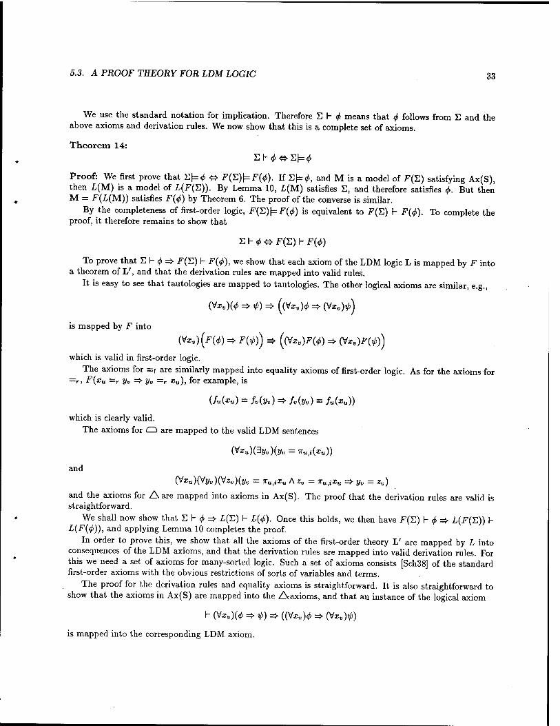
We use the standard notation for implication. Therefore E h <f> means that <j> follows from E and the above axioms and derivation rules. We now show that this is a complete set of axioms.
Theorem 14:
Proof: We first prove that Y,\=(j> «> F(E)|=F(^). If E^, and M is a model of F(E) satisfying Ax(S), then L(M) is a model of L{F(Y,)). By Lemma 10, L(M) satisfies E, and therefore satisfies <j>. But then M = F(L(M)) satisfies F(<f>) by Theorem 6. The proof of the converse is similar.
By the completeness of first-order logic, F(Y,)\=F{4>) is equivalent to F(E) h F(<f>). To complete the proof, it therefore remains to show that
Eh^o F(E) r- F(^)
To prove that Eh^ f (E) h .F(^), we show that each axiom of the LDM logic L is mapped by F into a theorem of L', and that the derivation rules are mapped into valid rules.
It is easy to see that tautologies are mapped to tautologies. The other logical axioms are similar, e.g.,
(V*„)(* =>*)=*- ((V*„)tf => (Vz„)V>)
is mapped by F into
(V*„)(*"(*) => F(tf)) => (Wxv)F(4>) =» (Vaj^W)
which is valid in first-order logic.
The axioms for =, are similarly mapped into equality axioms of first-order logic. As for the axioms for =r, F(xu =r yv =» yv =r xu), for example, is
(fu(xu) = fv(yv) => fv(y«) = /«(*„))
which is clearly valid. The axioms for O are mapped to the valid LDM sentences
(Vxu)(3yv)(yv = xU|i(a;u))
and
(Va:u)(V!/u)(Vzu)(j/„ = TUiia;u A zv = Tu>ixu => yv = zv)
and the axioms for A are mapped into axioms in Ax(S). The proof that the derivation rules are valid is straightforward.
We shall now show that Eh^ 1(E) h L(4>). Once this holds, we then have F(E) h <j> => L(F(£)) h L(F{4>)), and applying Lemma 10 completes the proof.
In order to prove this, we show that all the axioms of the first-order theory L' are mapped by L into consequences of the LDM axioms, and that the derivation rules are mapped into valid derivation rules. For this we need a set of axioms for many-sorted logic. Such a set of axioms consists [Sch38] of the standard first-order axioms with the obvious restrictions of sorts of variables and terms.
The proof for the derivation rules and equality axioms is straightforward. It is also straightforward to show that the axioms in Ax(S) are mapped into the Aaxioms, and that an instance of the logical axiom
I- (Vxv)(<j> => V) => ((V*0)^ => (V*„)tf)
is mapped into the corresponding LDM axiom.

34 CHAPTER 5. THE LDM LOGIC
The remaining, and most difficult, case is the logical axiom
i- (v*„w*„) => m where t is a term that contains no variables that are quantified in <f> by a quantifier that has a free occurrence of xv in its range. This is mapped into the formula r- (Vxv)L(<j>(xv)) =* L(^>(t)). This might appear to be an instance of the corresponding LDM axiom, but it is not. The reason for this is that substituting t and then applying L does not give the same formula as applying L and then substituting t for xv. _
Let ^ be the result of substituting the term t for xv in <j>. We shall prove that (Vxv)(L(<f>)) =>■ L(<j>) is a theorem of LDM logic by showing, by induction on the size of <f>, that the stronger assertion (Vxv)(L(4>)) => LQ>) =>■ (3xv)(L(<f>)) is such a theorem. The proofs of all of the cases except when <f> is atomic are trivial. Note that the second implication is needed for the proof of the first implication to go through in the case of negation.
For the case when 4> is atomic, note first that v cannot be of sort c, since there are no variables of this sort. The treatment of the various types of atomic formulas are all similar, and we shall prove the result for the case when <j> is the formula xv £ yw- t must be a term of the form KVTVI • • -x„n(zu). (Wxv)L(<f>) is then the formula
(Vxv)(xv ewyw)
L(<f>) is the formula
(3a;t,)(3a;„1) • • • (3xVn)(xv irv xVl A • • • A xVn *■„„ zu A xv G«, yw)
and (3xv)L(4>) is (3xv)(xv €w yw). Proving the induction hypothesis is now straightforward since the LDM axioms for O-nodes imply that for each zu there are a?„n, ..., xVl, xv satisfying
(xv TV xVl A • • • A xVn x„n zu) |
Corollary 15: The axiom system introduced in this section is sound and complete for LDM logic. |
5.4. The Complexity of Integrity Checking
From now on we consider only instances that correspond to real databases. In other words all instance are finite, all 1-values are natural numbers, all r-values in nodes of type □ are from a fixed set D, and we do not distinguish between individual constants in the Schemas and data elements.
In this section we investigate the complexity of checking integrity constraints. The integrity constraints are sentences in LDM-logic, and a database is "legal" if and only if it satisfies the constraints. Following [Var82], we use two measures of complexity, data complexity and expression complexity. Intuitively, data complexity is the complexity of testing satisfaction of a fixed sentence in terms of the size of the database. Expression complexity, on the other hand, is the complexity of testing satisfaction of sentences on a fixed database in terms of the length of the sentences.
More formally, the data complexity of LDM logic is the complexity of the sets
GV(S, <j>) = {111 is an instance of S and (= j </>}
where <f> is a sentence over S. The expression complexity of LDM logic is the complexity of the sets
CV(S,I) = {«H 1=^}
where I is an instance of S. Note that Gr(S, <j>) is a set of instances, while GV(S, I) is a set of sentences.

5.4. THE COMPLEXITY OF INTEGRITY CHECKING 35
Theorem 16:
1. For every sentence <f> over S, the set Gr(S,<f>) is in LOGSPACE.
2. For every instance I of S, the set Gr'(S,I) is in PSPACE.
3. There is a schema S and an instance I of S, such that the set Gr'(S, I) is logspace complete in PSPACE.
Proof:
1. We have to test whether, for a fixed sentence <j>, |= j <j>. Let \I\ = n be the number of 1-values in I, and let k be the number of quantifiers in <f>. In order to test whether \= j <j>, we have to test all possible assignments of values to these variables, of which there are at most ra*. If we cycle through these assignments in a fixed, say lexicographic, order, we can do this in space 0(klogn) = O(logn). For each such assignment it is easy to see that testing <f> takes constant space.
2. As in the previous case, we can test |=j <f> in 0(k\ogn) = 0(k) space. In this case n is fixed and ib, the number of quantifiers in <f>, is less than the length of <j>.
3. We shall reduce the Quantified Boolean Formulas (QBF) of [Sto77] to the set GV'(S,I). Let S be the schema consisting of the single node u of type D. Let I be the instance of S with I(u) = {1,2} and r(l) = F, r(2) = T. If E' = (Qi^i) • • • (Qnx„)E is an instance of QBF, let <f>{E') be the LDM formula that we get by replacing each literal x< in E by x'u =r T, each ~ffu by x*u =r F, and each quantifier (QiXi) by (Qixi). We clearly have |<£(£")| = c\E'\, and also
^')GGr'(S,I)ohl^')
O There exists a satisfying truth assignment for E' |
Thus the data complexity of LDM logic is LOGSPACE, and the expression complexity of LDM logic is PSPACE. Since analogous results hold for the relational model [Var82], we see that integrity checking in the logical data model is not more difficult than in the relational model.
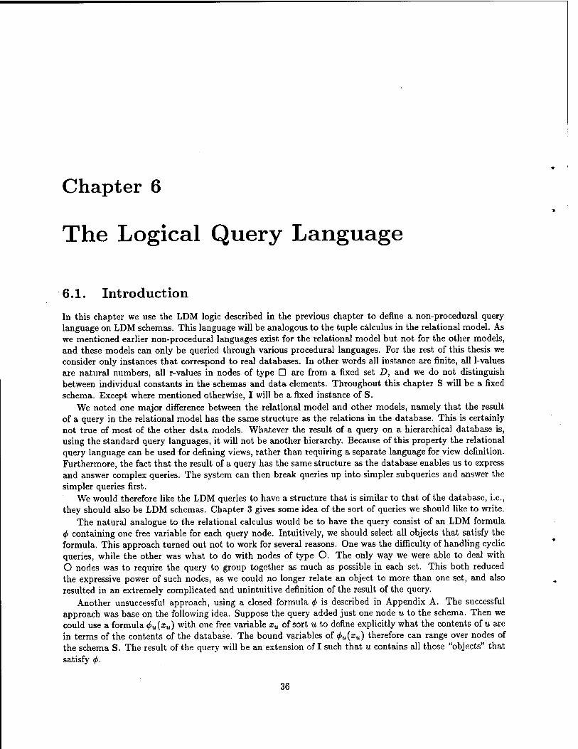
Chapter 6
The Logical Query Language
6.1. Introduction
In this chapter we use the LDM logic described in the previous chapter to define a non-procedural query language on LDM Schemas. This language will be analogous to the tuple calculus in the relational model. As we mentioned earlier non-procedural languages exist for the relational model but not for the other models, and these models can only be queried through various procedural languages. For the rest of this thesis we consider only instances that correspond to real databases. In other words all instance are finite, all 1-values are natural numbers, all r-values in nodes of type D are from a fixed set D, and we do not distinguish between individual constants in the Schemas and data elements. Throughout this chapter S will be a fixed schema. Except where mentioned otherwise, I will be a fixed instance of S.
We noted one major difference between the relational model and other models, namely that the result of a query in the relational model has the same structure as the relations in the database. This is certainly not true of most of the other data models. Whatever the result of a query on a hierarchical database is, using the standard query languages, it will not be another hierarchy. Because of this property the relational query language can be used for defining views, rather than requiring a separate language for view definition. Furthermore, the fact that the result of a query has the same structure as the database enables us to express and answer complex queries. The system can then break queries up into simpler sub queries and answer the simpler queries first.
We would therefore like the LDM queries to have a structure that is similar to that of the database, i.e., they should also be LDM Schemas. Chapter 3 gives some idea of the sort of queries we should like to write.
The natural analogue to the relational calculus would be to have the query consist of an LDM formula <j> containing one free variable for each query node. Intuitively, we should select all objects that satisfy the formula. This approach turned out not to work for several reasons. One was the difficulty of handling cyclic queries, while the other was what to do with nodes of type O. The only way we were able to deal with O nodes was to require the query to group together as much as possible in each set. This both reduced the expressive power of such nodes, as we could no longer relate an object to more than one set, and also resulted in an extremely complicated and unintuitive definition of the result of the query.
Another unsuccessful approach, using a closed formula <j> is described in Appendix A. The successful approach was base on the following idea. Suppose the query added just one node u to the schema. Then we could use a formula ^u(^u) with one free variable xu of sort u to define explicitly what the contents of u are in terms of the contents of the database. The bound variables of <j>u(xu) therefore can range over nodes of the schema S. The result of the query will be an extension of I such that u contains all those "objects" that satisfy <f>.
36

6.2. THE LDM QUERY LANGUAGE 37
What do we do if Q adds more than one node to S? We decided to extend this approach by having one formula per node. Each such formula will define the result at its node in terms of the contents of the database and of nodes whose result has already been constructed. A consequence of this is that the query schema must be acyclic. As we still allow the database schema to be cyclic and only prevent the user from constructing new cycles in his queries we do not think that this is too serious a restriction.
6.2. The LDM Query Language
Definition 23: Let S = (V, E,ß) be an LDM schema. A query on S consists of a tuple Q = (SQ, $Q, -<Q)
where
1. SQ is an extension of S.
2. -<Q is a topological order on the nodes in VQ - V, i.e., -<Q is a linear order such that if v is a child of w then v -<Q W.
3. <3>Q is a set of LDM formulas, one for each node v in VQ - V. The formula 4>v that corresponds to the node v satisfies
(a) 4>v has only one free variable, and it is of sort v.
(b) All other variables in <j>v are bound. Each of their sorts is either a node of the database schema S or is a query node that precedes v under -<Q.
The order -<Q is used to specify the order in which we define the result of the query. In Section 6.4 we investigate to what extent we can do without this order.
Before continuing with the formal details we give several examples of logical queries. The database schema in these examples will be the genealogy schema of Fig. 8 (page 10). The instance of it will be that shown in Fig. 10 (page 11).
Example 12: The schema of Qi is shown in Fig. 22, The formula <f>u>(xu>) is (Byu)(xu< =r yu). In other words we want I{u') to be a copy of I(u). We eliminate, however, any duplication that may be in I(u). The result of the query1 is shown in Fig. 23.
«'□
Figure 22: Schema of Qi
In all these examples, the result is denned only up to isomorphism relative to S, i.e., the choice of 1-values is arbitrary

38 CHAPTER 6. THE LOGICAL QUERY LANGUAGE
/(«')
I r(/) 17 Rehoboam 18 Solomon 19 David 20 Batsheba 21 Jesse
Figure 23: Result of Qi
Example 13: The schema of Q2 is shown in Fig. 24. Q2 has <£u'(av) always true. The result is quite large containing 26 = 64 elements, the 1-values 17 to 80. For this reason we do not show it here. The r-values of these 1-values are all the subsets of I(u).
Figure 24: Schema of Q2
Example 14: The schema of Q3 is shown Fig. 25. We want v' to contain the set of parents of Solomon and so we have the formulas
<M*«<) = (3tfi)(3^)(3zB1)(3z0
2)(3z2)((»i =r av) A {y2u =r «Solomon»)
A(z„2 =r {vl, 4)) A K1 G 4) A (tfi xi zl))
and <f>vi(xvi) = (Vyu/)(2/u/ € a:«')- What <£u'(av) says is that there is some 1-value (yl) in I(u) with the r-value "Solomon," and another
(2/i) with r-value equal to xui. The rest of the formulasays that j/i is a parent of y„. <j>v\xvi) says that I(v') contains all the 1-values in J(u') in one set. The result of the query is shown in Fig. 26.
Example 15: The schema of Q4 is shown in Fig. 27. We want to restructure the hierarchy as a relation, i.e., we want I(v') and I(w') to contain all the names of people that are in the database and J(u') to connect people to their parents. The formulas are
4>v>(xvi) = (3yu)(av =r Vu)

6.2. THE LDM QUERY LANGUAGE 39
o
17 18
Figure 25: Schema of Q3
r(0
/(</)
David Batsheba
19 -(0
{17,18}
Figure 26: Result of Q3
<f>w'(xw>) = (3yu)(sc««,< =r J/u)
and
M*«') = (3xJ,)(3^,)(3j,i)(3^)(34)(3^2)(34)((^' =r tfi) A (4- =r fi)
A(*i» =r (4> 4')) A (4 =r (j/i , 4)) A (j/2 Tl 22) A ^ g z3 jj
The result of the query is shown in Fig. 28.
We now formally define the result of a logical query. We start by looking at queries that add just one node to the schema. We shall call queries like this simple queries.
Definition 24: A query Q is called a simple query if
simple query that has VQ — V = {«}. VQ-V = 1. We shall use the notation Q„ for a
Let Q„ be a simple query on a schema S and let I be an instance of S. The result of Q„ on I will be an extension I„ of I to SQ . In order to define I„ we have to define what Iv(v) is and what the r-values of these 1-values are. It should contain all those "objects" that satisfy 4>v(xv). The problem with using this as a definition of I„ is that <j>v(xv) is satisfied by 1-values and since Iv(v) has not yet been defined it is meaningless to talk about the objects that satisfy <f>v. It might seem that problem is trivial, but suppose that <j>v(xv) included the conjunct (V«/„)(Vz„)(j/„ =/ zv). In other words I(v) can contain at most one 1-value. If the rest of 4>v allowed several possibilities for the r-value of this 1-value we would have no way of choosing which one would be in the result.
What enables us to deal with this problem is that a formula like this is not allowed in our query language— all bound variables in our language must refer to database nodes or nodes that precede v, not to v itself. As a result of this restriction, it will turn out that although <f>v refers to 1-values, it really expresses something about their r-values alone. This will enable us to find the r-values that satisfy <f>„ and after that pick the 1-values arbitrarily.
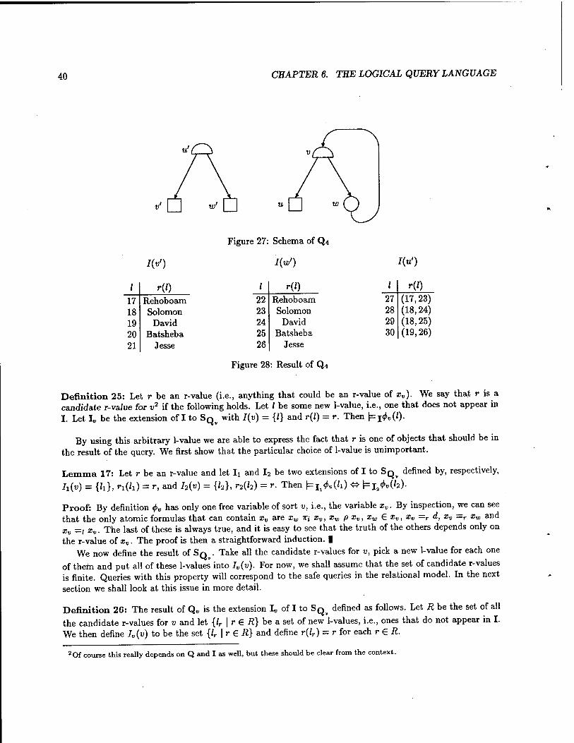
40 CHAPTER 6. THE LOGICAL QUERY LANGUAGE
u'O
I(v')
Figure 27: Schema of Q4
I(w>)
I r(0 17 Rehoboam 18 Solomon 19 David 20 Batsheba 21 Jesse
/ r(0 22 Rehoboam 23 Solomon 24 David 25 Batsheba 26 Jesse
I(u>)
I r(0 27 28 29 30
(17,23) (18,24) (18,25) (19,26)
Figure 28: Result of Q4
Definition 25: Let r be an r-value (i.e., anything that could be an r-value of xv). We say that r is a candidate r-vaJue for v2 if the following holds. Let / be some new 1-value, i.e., one that does not appear in I. Let I„ be the extension of I to SQV with I(v) = {1} and r(l) = r. Then t=I<M0-
By using this arbitrary 1-value we are able to express the fact that r is one of objects that should be in the result of the query. We first show that the particular choice of 1-value is unimportant.
Lemma 17: Let r be an r-value and let Ii and I2 be two extensions of I to SQ^ defined by, respectively,
h{v) = {h}, n(h) = r, and J2(«) = {/2}, r2(l2) = r. Then t=I1^('i) ^ Nl^a)-
Proof: By definition <j>v has only one free variable of sort v, i.e., the variable xv. By inspection, we can see that the only atomic formulas that can contain xv are xw 7r< xv, xw p xv, xw e xv, xv =r d, xv —r xw and xv =1 xv. The last of these is always true, and it is easy to see that the truth of the others depends only on the r-value of xv. The proof is then a straightforward induction. |
We now define the result of SQV. Take all the candidate r-values for v, pick a new 1-value for each one of them and put all of these 1-values into Iv(v). For now, we shall assume that the set of candidate r-values is finite. Queries with this property will correspond to the safe queries in the relational model. In the next section we shall look at this issue in more detail.
Definition 26: The result of Q„ is the extension I„ of I to SQ^ defined as follows. Let R be the set of all the candidate r-values for v and let {/r | r € R} be a set of new 1-values, i.e., ones that do not appear in I. We then define Iv(v) to be the set {/r | r G R} and define r(lr) = r for each r € R.
2 Of course this really depends on Q and I as well, but these should be clear from the context.
6.2. THE LDM QUERY LANGUAGE 41
We now show that this definition has the properties we want. We show that the result is well defined (up to isomorphism relative to S, and assuming finiteness), that everything in the result satisfies <j>v and that we cannot add anything else that satisfies 4>v to the result without introducing duplication. Some of this formalizes what we meant when we said that <f>v expresses something about the r-values of xv rather about than their 1-values.
We first state a lemma which we shall need for the proof of Lemma 19. The proof of this lemma is similar to the proof of Lemma 17.
Lemma 18: Let I2 be an extension of I to SQ . Let I be an element of Ii(v) and let I2 be the extension of I to SQv defined by I2(v) = {/} and r2(l) = r\(l). Then 1=1,6,(0 <» l=I2<M0- ■
Lemma 19:
1. Let Ii and I2 be two results of Q„. Then Ii and I2 are isomorphic relative to S.
2. Let I„ be the result of SQ . Then for each / in Iv(v), \=iv4>v(1)-
Proof:
1. Let Ii and I2 be two possible results of Q and let h be an element of I^v). Since r(li) is a candidate r-value for v there must be some /2 in I2(v) with r(l2) = r(h). Since both I^v) and I2{v) have no duplication we immediately get a 1-1 correspondence between the 1-values of h(v) and h{v). It is easy to see that this correspondence is an isomorphism.
2. Let / be an arbitrary element of Iv(v), and let I* = (I*,r*) be the extension of I to SQ defined by I*(v) = {/} and r*(l) = r(l). By Lemma 18
hiXO^hi.MO Since r(l) is a candidate r-value for v we can extend I to an instance I** of SQ by defining I**(v) = {/*♦}, r**(l**) = r(l), for some new 1-value /•*. We then have (=!..<£„(/**). By "Lemma 17, hl.<M0 and therefore \=j<f>v(l). |
We now define the result of an arbitrary query Q. To do this, we first define composition of queries.
Definition 27: Let Qi be a query and let Q2 be a query on SQ^ Q2 O QJ is the query on S that we get by composing them, i.e., Q2 o Qj has SQ20QI = SQ^, *Q20QI ='^Q1 U^Q2 and
•^Q.oQ^^Q, U -^Q2 U {(«,«,) | v G VQI(«, 6 VQJ
Lemma 20: Q2 o Q1 is a query on S. |
Let the nodes added by the query Q be VQ - V = {vi,..., vn} where vt -< ivn. We shall define a sequence of simple queries QUl, ..., Q„B, as follows. Each Q„. is a query on the schema of QVi_t and adds the node vt to that schema. The formula for vt is <f>V{. It is easy to see that Q = Q^ o • • • o QVl and this enables us to easily define the result of Q.
Definition 28: The result of the query Q on I is the result of applying the queries QWl,..., QVn successively to I.
Lemma 21: The result of Q is well defined, i.e., different choices of 1-values at each step yield isomorphic results.

42 CHAPTER 6. THE LOGICAL QUERY LANGUAGE
Proof: This is a straightforward application of the first part of Lemma 19. I The following theorem shows that the result of the query has the desired properties. These include a close
relation with the maximize data while minimizing duplication approach that we described in the previous section.
Theorem 22: Let IQ be the result of the query Q on the instance I
1. Let v be a node added by Q and let I be an element of I(v). Then (=j^„(/).
2. If v is a node added by Q and k and l2 are two different 1-values in I(v) then r(h) £ r(l2). In other words there is no duplication in the result.
3. I„ is a maximal extension of I to SQ that satisfies 1-2, i.e., there is no extension IJ with I*(v) D Iv(v) for all v € VQ - V that satisfies 1-2 and such that for at least one v the inclusion is proper.
Proof:
1. Let Q* be the query Q„„ o • • • o QWl where v = vk and let IQ. be the result of Q*. By Lemma 19, |= j 4>v(l). It is easy to see that I is an extension of an isomorphic image of IQ and that extending
1^ to SQ does not affect the satisfaction of<f>v.
2. Obvious.
3. Assume that such an I* exists. Let v = vk be the first of the nodes Vi, ..., vn for which I* (v) £ Iv (v) and let Q* be the query QVh o • • • o Q^. From 1 and 2 it follows immediately that both I„ and IJ restricted to SQ. are results of Q*. Lemma 21 then implies that IJ and I„ are isomorphic, a
contradiction. |
6.3. Safe Queries
We have seen that provided that the set of candidate r-values at each node is finite, the result of the query is well-defined. It remains to see when the set of candidate r-values is finite.
Definition 29: A query Q on a schema S is safe if for every instance I öf S, the set of candidate r-values at each node, under the construction described above, is finite.
Note that as we are considering only finite instances, this is the same as requiring that the query have a result on every database instance.
Let «bea query node, i.e., an element of VQ - V. Assume that we have defined the result of Q for
all those nodes that precede v. If n{v) - O, O or A the set of candidate r-values for v is contained in either the cartesian product, union or powerset of the instance(s) of its child(ren) and therefore must be finite. The only case when it may be infinite is when fj,(v) = D. If the domain D of data is finite, then all queries are safe, since the set of candidate r-values for nodes of type D is a subset of D. We therefore assume throughout this section that D is infinite.
Lemma 23: Q is safe on I iff for every query node of type D the set of candidate r-values for v is finite. |
We give two examples using the database and query schema shown in Fig. 22 (page 37) and the database instance shown in Fig. 10 (page 11).
6.3. SAFE QUERIES 43
Example 16: <f>u'(xu>) is (3j/u)(av =r y«) V (av =r "Absalom"). This query is safe since the set of candidate r-values is R = { Jesse, David, Batsheba, Solomon, Rehoboam, Absalom}.
Example 17: <f>u'(xu') is (xu> #r "David"). This query is unsafe since the set of candidate r-values is R = D — {David}, an infinite set.
As we have pointed out above, testing whether a relational query is safe is undecidable. As we can reduce testing safety of relational queries to testing safety of LDM queries there cannot be a decision procedure that tells us whether an query is safe on all database instances.
We give, however, a decision procedure for safety on fixed instances. Let I be a fixed instance of S and let Q be a query on S.
Lemma 24: Let w\,..., wn be all of the nodes in the schema S that are of type D and let {di,..., dk} be the constants that occur in any of the query formulas. Q is safe on I iff for each query node v of type D, every candidate r-value for v is either a) the r-value of an element of some /(to,) or b) one of the dj's.
Proof: One direction is obvious—if this condition holds then Q is safe on I. We prove the converse by induction on the query nodes VQ - V = {«i,.. .,«„} where «i -<•••-< w„. Let v = vt be a query node of
type D. We assume that the lemma holds for the nodes that precede Vi and that the query is safe on I. Let I,_i be the result of Qo^.
Since Q„ is safe on I the set of candidate r-values for v is a finite set R. We have to show that
AC {<*!,...,<fc}U (J I(w)
ß(w) = D w € V
Call the right hand of this equation S. If the lemma is false, then there is some element r in R — S. By the induction hypothesis
S={d1,...,dk}\J (J /,-_!(«,)
P(W) = a w e V or
w G VQ ,w -iv
Since r is a candidate r-value for v, if we extend Ij_i to an instance 1} of SQ by defining J/(u) = {/} and
ri(0 = r, we have |=ii<^«(/). Let r' be an arbitrary element of D - S, and extend Ij_i to an instance I? of SQv by defininS lHv) = {0 and r2(0 = r'. Since r and r' do not appear in the database, previously constructed nodes, or in the query formulas, an induction shows that
r=Ii^»(0<»r=Ij^t;(0
The key point in the induction is that xv can occur in <j>v(xv) only in atomic formulas of the form xv =r dj and xv =r yw, where w is a node of type D that is either in V or is one of the nodes vi !;,_! The only other atomic formulas that can involve x„ are xv =/ a;„ and xv =r xv, and these are always true. All these formulas are false whenever the r-value of xv is not in S.
We have therefore shown that all the elements of the infinite set D - S are candidate r-values, a contradic- tion. |
The technique of this proof gives us an effective procedure for determining whether the simple query Q„ is safe on the instance I. Take some constant d0 that does not occur anywhere in the database or in the query formulas. Test it d0 is a candidate r-value (it is not difficult to see that this can be done effectively).

44 CHAPTER 6. THE LOGICAL QUERY LANGUAGE
In a similar way to the proof of the above lemma, we can show that Q„ is safe on I iff dQ is not a candidate r-value for v. Intuitively, if some such d0 is in the result, the result is infinite since d0 cannot be distinguished from any other such constant.
Combining this result with those of the previous section we get:
Theorem 25: Let Q be a query on S and let I be an instance of S. There is a decision procedure to test whether Q is safe on I. If Q is safe on I then the result can be computed effectively. |
Even though testing for safety and computing the result can be done effectively, it can still be NP-hard to do so, as we shall see in Section6.5.
6.4. Ordering the Nodes in a Query
We now examine more closely the role of the topological order in an LDM query. It might seem at first that we can relax the requirement. If each <j>v referred only to database nodes and to descendants of v, we could evaluate the query "bottom-up" without having to specify explicitly the evaluation order as part of the query.
Let us call the query language we would then get the bottom-up query language. The reason we prefer the LDM query language to the bottom-up query language is that the bottom-up language is not closed under composition.
The reason it is not is as follows. Let Q2 be a query on the result of Qi. Then the formula for a node v in Q2 can refer to a node u in Qi that is not a descendant of v. This by itself does not necessarily mean that the language is not closed under composition—we might be able to rewrite the formula <j>v to get an equivalent query that does not refer to u. For example, if u is of type O we can rewrite <f>v to refer only to the descendants of u. We now show that if u is of type O this cannot always we done.
Theorem 26: The bottom-up query language is not closed under composition.
Proof: The database schema S consists of the node v in Fig. 29. Qi adds the nodes u and w, and Q2 adds the node t to the result of Qi.
«D Figure 29: Query used in the proof of Theorem 26
The outline of the proof is as follows. We first show how by a suitable definition of Qi and Q2 we can get I(t) to contain copies of exactly those r-values in I(v) that occur with the most duplication. If there were a bottom-up query equivalent to Q2 o Qj, it would have to define I(t) in terms of database nodes and descendants of t, i.e. in terms of I(v), alone. In the second part of the proof we show that this cannot be done.
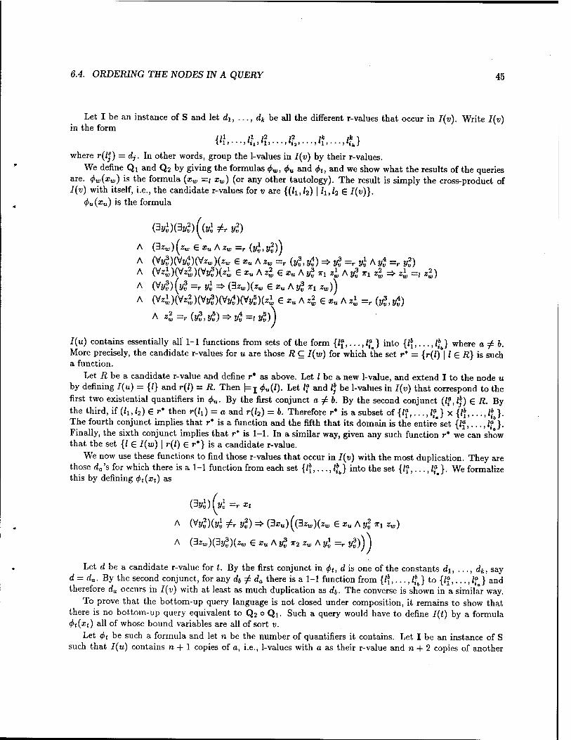
6.4. ORDERING THE NODES IN A QUERY 45
Let I be an instance of S and let di, ..., dk be all the different r-values that occur in I(v). Write I(v) in the form
Vii • • •)«»!)'!> • • -.'»ai • • -,h> ■ ■ ->hk}
where r(/j) = dj. In other words, group the 1-values in I(v) by their r-values. We define Qx and Q2 by giving the formulas <f>w, <pv and <j>t, and we show what the results of the queries
are. <j>w(xw) is the formula (xw =; xw) (or any other tautology). The result is simply the cross-product of I(v) with itself, i.e., the candidate r-values for v are {(h,h) \ h,h G I(v)}.
4>u(zu) is the formula
A (3zw) (zw £xuAzw =r (yl, y%))
A (Vy„3)(Vy„4)(V^)(^ e xu A zw =r (yg, rf) => tf =r £ A y*v =r y„2) A (v4)(v4)(Vj/?)(4 e *« A 4 e *„ A »J X! 4 A »g X! 4 => 4 =, 4) A (VyjJ) (yg =r yi =>■ (3zw)(zw G zu A yg xx z«,))
A (V4)(V4)(Vy?)(V^)(Vy„5)(4 G *u A 4 € xu A 4 =r (y?, rf)
/(w) contains essentially all 1-1 functions from sets of the form {If,..., IfJ into {/*,..., /,• J where a ^ b. More precisely, the candidate r-values for it are those R C I(w) for which the set r* = {r(/) | / G R} is such a function.
Let Äbea candidate r-value and define r* as above. Let / be a new 1-value, and extend I to the node u by defining I(u) = {/} and r(l) = R. Then f=j <f>u(l). Let If and l) be 1-values in I(v) that correspond to the first two existential quantifiers in <f>u. By the first conjunct a^b. By the second conjunct (/?,/}) G R. By the third, if (h, /2) G r* then r(h) = o and r(/2) = 6. Therefore r* is a subset of {/?,..., IfJ x {l\,..., /fj. The fourth conjunct implies that r* is a function and the fifth that its domain is the entire" set {/",■..., if}. Finally, the sixth conjunct implies that r* is 1-1. In a similar way, given any such function r* we can show that the set {/ G I(w) \ r(l) G r*} is a candidate r-value.
We now use these functions to find those r-values that occur in I(v) with the most duplication. They are those rfa's for which there is a 1-1 function from each set {/*,...,/*J into the set {/?,.. .,/?„}. We formalize this by defining <j>t{xt) as
A (Vy^)(yi ±r y2) => (3xu)((3zw)(zw G *u A y2 xx zw)
A (3zw)(3y*)(zw exuAy^T2zwAyl =r yg)) j
Let rfbea candidate r-value for t. By the first conjunct in <j>t, d is one of the constants dx, ..., dk, say d = da. By the second conjunct, for any db ^ da there is a 1-1 function from {/f,..., ZfJ to {If, ...,lfa} and therefore da occurs in I(v) with at least as much duplication as dj. The converse is shown in a similar way.
To prove that the bottom-up query language is not closed under composition, it remains to show that there is no bottom-up query equivalent to Q2 o Qj. Such a query would have to define I(t) by a formula (f>t(xt) all of whose bound variables are all of sort v.
Let (j)t be such a formula and let n be the number of quantifiers it contains. Let I be an instance of S such that I(u) contains n + 1 copies of a, i.e., 1-values with a as their r-value and n + 2 copies of another

46 CHAPTER 6. THE LOGICAL QUERY LANGUAGE
constant 6. Let I* be a second instance of S, that differs from I only by containing another copy of a, i.e., another 1-value /* with r-value a. Then the only candidate r-values for t on I should be b and both a and b should be candidate r-values on I*.
Let /( be a new 1-value. Extend both I and I* to t by denning I(t) = I*(t) = {/<} and r(lt) = r*(lt) = a. We shall complete the proof by showing that (=j <f>t(lt) ■& hl*&(**) and thus contradicting the fact that a is a candidate r-value for t on I* and not on I.
Let the free variables of <j> be among the variables xt, x], ..., xn. We prove the following by induction. Let Zjfc+i, ...,/„, or any other subset of the /<'s be elements of I(v). Let 1 be any element of I(v) distinct
from /jfc+i, ..., ln that satisfies r(/) = a. Then
1=!.^,/*,... ,/Vt+i,... ,ln)&\=i<f>(h, I,... ,/,/*+!,...,/„)
(Note that /* is the 1-value that appears in I* but not in I.) Using this with 4> = 4>t will complete the proof. When <f> is an atomic formula or ->^i or <f>i A <f>2 the proofs of this assertion is straightforward. The hard
case is when <f> is (W„)^){xt, x\,..., x%). Given a set A C I(v) we shall say that / is suitable for A if r(l) = a and I is not an element of A. If 1 is suitable for A andsome / € A has r-value a, it is easy to see that / is suitable for A - {1} U {/}. The assertion says that if 7 is suitable for {/jt+i,..., /„} then the equivalence holds. Since I(v) has n + 1 copies of a, we can always find at least two suitable 1-values for any set A of size less than n.
To show the first direction, let 1 be suitable for {/*+i,..., /„} and assume that
Since the value assigned to the quantified variable x*v is irrelevant, assume, w.l.o.g., that i > k + 1. For all loeI(v)CI*(v), hj.M.JV ...JVt+i, ...,'o,. •-,'»)
1. If l0 ^ 7, then I is suitable for {h+i, ■■-,ln}- The induction hypothesis then implies that
hi 0(Jtif|--->M*+l»- ■•,k,---,ln)
2. Replacing the quantified variable by /*, we get
Since 1 is suitable for {h+i, • • •, /t-i,'*+i» • • •, M the induction hypothesis implies
hi <f>(lt>l> •••>*. **+i> • • •, *i • • • i *n)
Combining these two, we get hi((v4)MU,...,U+i,...,M
For the converse, assume that [=j ((Vxj,)^)(it,Z,...,/,/fc+i,.. .,/„) holds. Then, for all l0 € I(v)
h I 4>{h, l, -J, h+i, • • • > 'o. • • •, 'n)
1. If /o 7^ h then I is suitable for {/o,'t+i, • • • ,h-i,U+i, ■ ■ •>'«} and therefore
(=I^('li'*i- •. '*» '* + l. ■■■,lo, ••■Jn)

6.4. ORDERING THE NODES IN A QUERY 47
2. If Z0 = 7, then 7 is suitable for {k+i,..., U-i, h+i,..., /„} and we get
hl.M, /*,...,/*,/*+!,... ,**,...,/„)
3. So far, we have shown that \=i,<j>{lt,l*,. ..,l*,lk+i,.. .,l0, ■■.,/«) for any /0 in /(v). Pick two 1-values /o and /Q that are both suitable for
{U*+i, • ..,h-i,li+i,...,ln}
Then /£, is suitable for {/0, h+i,..., U-i, /,+i,...,/«} and the induction assumption implies that
hi 4>(lt, l'o, ...Jo, h+i, ...,l0,...,ln)
IQ is suitable for {/(,, h+i, ■■■,h-i,U+i, ■•■Jn] and the induction hypothesis now gives us
hi« Mi C •••» '0. h+i, ...,/*,..., /„)
Using the induction assumption once more, together with the fact that 7 is suitable for
{'Of '*+l» - - -»'i—1. 't+1, • - Jn}
gives us \= j </>(h,l'0, ...,1'0, k+i, ...,/,...,/„) Finally we use the induction hypothesis another time, this time with the fact that 1'0 is suitable for
V Jk+l, ■ • .,/i_l,/*+!,...,/„}
to get \= j.tih,I*,...,I*,lk+l,...,l,...,ln).
Combining these shows that |= j. ((Vxi)(^)(/t ,/*,...,/*, /t+1 ,...,/„) and completes the proof. | As a consequence of this theorem we see that the topological order is a necessary part of the definition
of the LDM query language. However, this does not mean that the user has to explicitly specify the order as part of the query, since it is enough if he just specifies the formulas at the nodes of the query. The system can then pick some order on the query nodes that is consistent with the graph edges and the implicit dependencies of one formula on another, i.e., if the formula for v refers to the node u then u must precede v. If the query is a legal one such an order must exist. The specific order we pick, subject to these constraints, turns out to be irrelevant. The following theorem shows that if we pick a different ordering we would get an equivalent query.
Theorem 27: Let Ch = (SQ,XI,#^ and Q2 = ^SQ,-!2,$^ be two queries on a schema S that differ
only in the topological order. Let I be an instance of S. Then the results of Qj and Q2 on I are isomorphic relative to S.
Proof: Let Ii and I2 be the two results. Let the query nodes be VQ-V = {vx,..., vn} where vx -<! (1 vn. We define an isomorphism / from Ix to I2 by induction on the order -d. Assume / has been defined for all w such that w -<i v. Let R be the set of candidate r-values for v and write h(v) as {/r | r £ R). We first define a mapping /* on the candidate r-values for v as follows.
1. If/i(u) = D, then f*(r) = r.
2. If n(v) = (C2), n), then r is a tuple (h,..., ln) and we define

48 CHAPTER 6. THE LOGICAL QUERY LANGUAGE
3. If ß(v) = A then r is the 1-value I and we define f*(r) = /(/).
4. If n{v) = O, then r is a set and we define /*(r) = {/(/) |l£r}.
It is not hard to show that /*(r) is a candidate r-value for v in Q2. Somewhat informally, the proof is as follows. Let h(v) consist of the single 1-value k with r-value r and let I2(v) consist of the single 1-value l2 with r-value f*(r). Restrict the schema in both cases to the database S and those nodes that precede v in both Qi and Q2. We can then show that by defining f(h) = h we get an isomorphism between the instances. Theorem 3 then shows that /*(r) is a candidate r-value for v in Q2.
We can show in a similar way that the image of /* contains all the candidate r-values for v in Q2, and we can therefore write h(v) as {lr(r) \r€R} where r(lr(r)) = f*{r). By defining /(/r) = lf.(r) we get the desired isomorphism. |
6.5. Complexity of the Query Language
It is clear that the complexity of evaluating a query can be exponential, or worse, is the size of the database instance, since even the size of the result itself can be multiply exponential in the database size. We therefore ask the following question: Given a query and a database instance what is the complexity of testing whether the result is empty? We show that even this problem is NP-hard.
Theorem 28: Let Q be a query on a database with schema S and instance I. It is NP-hard to determine whether the result of Q on I is empty or not.
Proof: We reduce the problem to 3SAT [GJ79]. For the reduction we use the database and query Schemas shown in Fig. 30, where the database schema is in the box on the right. We describe informally how to map an instance of 3SAT into a database instance and what the query Q is.
Figure 30: Reduction from 3SAT
The instance I corresponding to an instance of 3SAT is defined as follows, u contains all the variables in the instance and v contains the two constants T and F. w contains all possible pairs (x, T). Finally, each set in t corresponds to a clause, where the pair (x, T) is interpreted as the variable x and (x, F) as the variable x.

6.5. COMPLEXITY OF THE QUERY LANGUAGE 49
Q is defined as follows. Each set in s corresponds to a satisfying truth assignment. In other words, such a set r must satisfy:
1. No two pairs (x,T) and (x,F) are in r. The pair (x,T) is now interpreted as assigning the value true to x.
2. For each x in u, either (x, T) or (x, F) is in r.
3. Each clause, i.e., each set {(x, a), (y, b), (z, c)} in t is "satisfied" by the members of s, i.e., at least one of (x, a), (y, b) and (2, c) is in r.
It should be clear that we can write a formal LDM query expressing these requirements. It is then easily seen that instances for which 3SAT has a solution are mapped into database instances for which the query has a nonempty result and then testing whether the result is empty shows whether the instance of 3SAT has a satisfying truth assignment. |
A modification of the above proof shows that it is also NP-hard to determine whether a query Q is safe on a given database instance I. To see this, let the database be as in the proof of the above theorem, and let Q add the node s above, followed by a node q of type D. The formula <j>s(x3) is as before, while <f>'q(xq) will just require that the result at the node s be nonempty, e.g., by the formula ^>q(xq) = (3xs)(xs =, xs). Note that <j>q does not mention the variable xq.
If we map instances of 3SAT into database instances as above, then whenever the instance of 3SAT has a satisfying truth assignment, the result at s is nonempty. In that case 4>q is satisfied by any 1-value, and the query is unsafe.
Conversely, whenever the instance of 3SAT has no satisfying truth assignment, the result at s is empty. But then 4>q is satisfied by no 1-value and therefore Q is safe. This shows that a test for safety can be used to test satisfiability, and therefore that the problem of testing a query for safety on a given instance is NP-hard.

Chapter 7
The Algebraic Query Language
7.1. The Algebraic Operators
In this section we define a complete set of algebraic operators. We shall then show that any safe logical query is equivalent to some sequence of algebraic operations. Conversely, each algebraic operation is equivalent to a safe logical query.
Since a logical query adds some nodes to the database schema and leaves the instance of the database schema unchanged, each algebraic operator must do the same. So a selection operator, for example, should not delete tuples that do not satisfy the selection condition, but should rather create a copy of the database node. That copy should contain only those tuples that satisfy the condition. In fact this copying of tuples is really what is done in the relational model—a query does not throw away those tuples in the database that do not meet a selection condition, but rather copies those tuples that do. This issue is not addressed explicitly in relational database theory, since the theory does not deal with what happens to temporary relations that are created while computing the result of a query.
In this section S will be a database schema with instance I. The algebra will consist of operations of the form w <— a(i>i,..., vn). Here a is the name of the operator, and its arguments vi, ..., v„ are nodes in the schema S. a adds the node w to the schema, and extends I to the new schema. We define each operator as a simple logical query. To define each operator we give
1. The types of its arguments.
2. The type of w and the list of its children.
3. An LDM formula <j>w(xw) that specifies the contents of I(w).
7.1.1. Operators that Copy and Combine Existing Nodes
1. w <- D(v) creates a copy of the node v, as is shown in Fig. 31. In all these figures the schema S is shown in the box on the right, and the node that is created by the operation is on the left. For each distinct r-value in I(v), I(w) will contain exactly one 1-value with this r-value. Note that duplication in I(v) is eliminated in I(w).
(a) v is a node of S that has type D.
(b) w is of type D.
(c) <f>w(xw) is (3yv)(xw =r yv)-
50
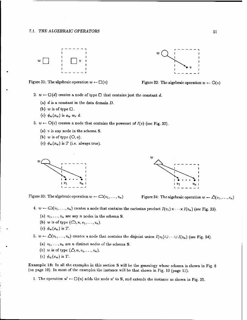
7.1. THE ALGEBRAIC OPERATORS 51
w D
Figure 31: The algebraic operation w <— D (v) Figure 32: The algebraic operation w <— 0(v)
2. w *— O (d) creates a node of type D that contains just the constant d.
(a) d is a constant in the data domain D.
(b) w is of type D.
(c) <f>w(xw) is xw =r d.
3. w *— 0(v) creates a node that contains the powerset of I(v) (see Fig. 32).
(a) v is any node in the schema S.
(b) w is of type (0,u).
(c) 4>w(xw) is T (i.e. always true).
wC^ w
Z\ i
t • • • • • 1 vi Vn
j
Figure 33: The algebraic operation w <— Q(ui,. ..,v„) Figure 34: The algebraic operation w *— £(vi >---,vn)
4. w <— C^(vi,. ..,vn) creates a node that contains the cartesian product I(vj.) x • • • x I(vn) (see Fig. 33).
(a) vi;...,v„ are any n nodes in the schema S.
(b) w is of type (O, n,vu.-., vn).
(c) <f>w(xw) is T.
5. w <— Z^ui,. ..,vn) creates a node that contains the disjoint union I(vi) U • • • U I(vn) (see Fig. 34).
(a) vi,..., vn are n distinct nodes of the schema S.
(b) w is of type (/S, n,vlt..., vn).
(c) <l>w(xw) is T.
Example 18: In all the examples in this section S will be the genealogy whose schema is shown in Fig. 8 (on page 10). In most of the examples the instance will be that shown in Fig. 10 (page 11).
1. The operation u' <— D(u) adds the node u' to S, and extends the instance as shown in Fig. 35.

52 CHAPTER 7. THE ALGEBRAIC QUERY LANGUAGE
2. For the remainder of this example, the database instance will be the smaller instance in Fig. 36. The result of the operation u' <- O(u) is the schema shown in Fig. 37, together with the instance shown in Fig. 38.
3. The result of the operation v' *- 0(u,t>) is the schema shown in Fig. 39, together with the instance in Fig. 40.
/(«')
/ r(l)
17 Rehoboam 18 Solomon 19 David 20 Batsheba 21 Jesse
Figure 35: Example of the algebraic operation u' <— D (u)
J(«)
I r(l)
I(v)
I r(l)
1 Batsheba
I(w)
I r(l)
2 (1,3) 3 0
Figure 36: A smaller instance of the genealogy schema
I(u>)
I r(l)
{Batsheba}
Figure 37: Example of the algebraic opera- tion u' <— O(u)
Figure 38: Result of v! <- O(u)

7.1. THE ALGEBRAIC OPERATORS 53
l(v')
/ r(l) 4 (1,2)
Figure 39: Example of the algebraic opera- tion v' <— 0(u, v) Figure 40: Result of the operation v'«- Q(u, v)
7.1.2. Selection Operators
The LDM algebra has two selection operators.
1. The operation w<r-<riej (v) is similar to the selection operation in the relational algebra. This operator selects those tuples in v whose ith and jth components are related by 9 (see Fig. 41).
(a) i) is a node of S of type (O, n,vu...,vn) and i 9 j is one of the relations i € j, i Tt j, i p j, i —i j and i =r j .
(b) u; is of type (O, »,«!,...,«„).
(c) 4>w(xw) is (3xv)(3yVi)(3yVi)(yVi irVi xv A yVj icVj xv A yVi 9 yVj A xv =r xw)
Alternatively, 9 may be of the form i =r d where d is a constant in D. Then <j>w{xw) is
(3xv)(3yVi)(yVi xVi xv AyVi =r dAxv =r xw)
w c^ w I
• V
:u
Figure 41: The algebraic operation w <— <n e j(v) Figure 42: The algebraic operation w <— o-in(u, v)
2. w <— am{u, v). Here u is a child of v, and w will contain those elements of I(u) that actually appear in /(?;), i.e., depending on the type of v, those elements of I(u) that occur either as members of sets, r-values or tuples (see Fig. 42).
(a) u and v are nodes of S and u is a child of v.

54 CHAPTER 7. THE ALGEBRAIC QUERY LANGUAGE
(b) w is of the same type as u and has the same children.
(c) <j>w{xw) depends on the type of v. Note that v cannot be of type D since it has a child u.
i. If v is of type O with u as its iih child then <l>w(xw) is
(3xu)(3xv)(xu =r Xw AXU Xj xv)
If there are multiple edges from v to u, we have to say which one we mean. In this case we shall use the notation crm(u, v, i) to mean: use the ith edge with tail v.
ii. If v is of type £s, then <f>w(xw) is
(3xu)(3xv)(xu =r xw A xu p xv)
iii. If v is of type O, then <j>w(xw) is
(3xu)(3xv)(xu =r xw A xu € xv)
Example 19: The schema continues to be that of Fig. 8 (page 10) and the instance is that of Table 10 (page 11).
1. The result of the operation u' <- 0-(1=r«Rehoboam")(u) is tne schema shown in Fig. 43, together with
the instance in Fig. 44.
2. The result of u' *- cr\n(w, v) is the schema in Fig. 45, and the instance in Table 46. Note that in this example u' is simply a copy of w, since every set in I(w) is a member of some tuple in I(v)
1 r(/)
Figure 43: Example of selection
15 (1,11)
Figure 44; Result of the operation u' <— 0"1=r"Rehobo
7.1.3. Union, Difference and Projection
1. The union operator is similar to the relational union. The syntax we use is w <— U(t>i,..., vn) (see Fig. 47).
(a) vi,...,vn are n nodes of S that are of the same type and have the same children.
(b) w has the same type and the same children as the u, 's.
(c) <j>w(xw) is (3xVl)(xVl -r xw) V • • • V (3xVn)(xVn =r xw).
2. For difference we shall use infix notation, i.e., we shall write w «- vi - v2 rather than -(^1,^2)-

7.1. THE ALGEBRAIC OPERATORS 55
/(«')
/ r(0 15 {7} 16 {8,9} 17 {10} 18 0
Figure 45: Example of the algebraic opera- tion u' <— <rin(w,v)
Figure 46: Result of the algebraic operation «' *-crin(w,v)
w •
w
o r
Figure 47: The algebraic operation to <— U(ui, v2) Figure 48: The algebraic operation w «- H{ Uli„3 }(u)
(a) vi and w2 are nodes of S that are of the same type and have the same children.
(b) w has the same type and the same children as vi and v2.
(c) </>w(*w) is (3ajSl)(jBUl =r xw) A (WxV2)(xVa ^r xw).
3. The projection operation is similar to projection in the relational algebra. The syntax we use is w <— HA(V), where A is an ordered multiset of edges with tail v.
(a) v is a node of S of type (Q, n,vu...,Vn) and A is an ordered multiset of edges with tail v.
(b) Let A = {eu ..., ek} where e, is the edge (v,«,-_.). Then w is of type (C2), k,vilt..., vik).
(c) <j>w(xw) is
(3a5«)(3a:«i) • ■ '(3a!».)(ir«jl TI a?« A • • ■ A (JB^ xt a?») A *„ =r (*„,,. ..,*„,))
When it will not cause any ambiguity, we shall use a set A of nodes rather than of edges, as in Fig. 48.

56 CHAPTER 7. THE ALGEBRAIC QUERY LANGUAGE
7.2. Equivalence of the Logical and Algebraic Query Languages
We can now use the algebraic operators defined in the previous section to define an algebraic query language. An algebraic query will be a sequence {au...,an} of algebraic operators, where each «i is an algebraic operator on the result of a<_i. We want to show that this query language is equivalent to the logical query language. In other words, for each logical query on a schema S, there should exist a sequence of algebraic operations, and vice versa, with the property that the schemas created by these two queries are identical, and for every database instance I, the results are isomorphic relative to S. Unfortunately, as the next example
shows, this is not quite true.
Example 20: Let S consist of a node u of type D and let Q be the logical query that adds a node v of type D to S. Let di and d2 be two distinct constants, and let <j>v(xv) be (xv =r dj. V xv =r d2). The candidate r-values for v are then {dud2}. There is no algebraic query equivalent to Q. If there was such a query, it would consist of one algebraic operation alone, since each operator adds a new node to the schema. By inspection we can see that no single algebraic operator is equivalent to Q.
How can we modify the definition to get an equivalent query? If QA is the algebraic query that consists of the operators Wl «- D(rfi), w2 *- D(d2) and v 4- U(u>i,u;2) it is clear that the instance of v is what we are after. If we were then to restrict the result of the query to the schema that consists of the nodes u and v we get the instance we want. We have essentially used the two nodes w1 and w2 for temporary storage while computing the result of the query. In fact the same thing occurs in the relational model, since temporary relations are used there for subexpressions and then deleted at the end. It is therefore reasonable to expect the same thing to happen in the logical data model.
To be able to use temporary nodes, we extend the algebraic query language by adding a "delete" operator. This operator will delete a node from the schema and restrict the instance of the original schema to the new schema. We have to make sure that we never delete a node that is the child of some other node, since in that case the result would not be a legal schema. The operator that deletes the node v will be written D(v).
Definition 30: Let S be an LDM schema with instance I. The algebraic operator D(v) is legal when v is a node with no parent. The result of D(v) is the schema S' that consists of deleting v from S, together with the instance that we get by restricting I to S'.
In the algebraic query language we must take care not to delete database nodes, i.e., we must only allow the user to delete nodes that have been constructed by his query. We shall call the language with the deletion operator the extended algebraic query language.
Definition 31: Let S be an LDM schema. An extended algebraic query on S is a sequence QA = (cti,..., a„) where each a* is either
1. An operation of the form wt <- ßi (v},..., «)'), where ft is an algebraic operator other than the deletion operator and v}, ..., v\j are either node of S or are nodes that were created by some previous ßj and have not been deleted.
2. The operator D(u,), where v, is a node that was created by a previous algebraic operator in the sequence ßi, .. ■, ßi-i and has not yet been deleted.
Definition 32: Let Q.4 be an extended algebraic query on S, and let QB be an extended algebraic query on the result of Q^. The query QB o QA is the composition of Q^ and QB, formed simply by concatenating
the lists of algebraic operators.
7.2. EQUIVALENCE OF THE LOGICAL AND ALGEBRAIC QUERY LANGUAGES 57
Obviously, the delete operator itself is not equivalent to any logical query, since every logical query adds nodes to the schema. This by itself does not necessarily mean that we cannot find a logical query equivalent to any extended algebraic query. After all, an extended algebraic query does not delete nodes of S, since the only nodes that are deleted are those that were constructed by previous algebraic operations. It might still be the case, as happened in Example 20, that there is an equivalent logical query that somehow expresses what the result of the query should be without using these temporary nodes.
At the end of this chapter (Theorem 36) we shall prove that such a query does not exist, thus showing that the extended algebraic query language is strictly more powerful than the logical query language. We can get equivalence by a simple modification of the logical query language: Allow logical queries to use temporary nodes as well.
Definition 33: Let S be an LDM schema. An extended logical query on S is a tuple Q = (SQ,$Q, -<Q, DQ)
where
1. ^5q,$Q,-<Qy is a logical query on S.
2. DQ is the set of temporary nodes used in the query. DQ is a subset of the query nodes VQ - V that we can delete and still get an LDM schema. In other words, there is no edge with tail outside DQ and head in DQ, i.e., if (ei,e2) G EQ and e2 G DQ then ex G DQ.
Definition 34: Let Q be the extended logical query Q = (SQ, $Q, <Q, DQJ, and let I be an instance of S. The result of this query consists of
1. The schema SQ consisting of
(a) The nodes in VQ — DQ .
(b) The relevant edges, i.e., all those edges of SQ whose head and tail are both in VQ - DQ.
(c) The restriction of the type assignment fj, to VQ - DQ .
2. The result of Q on I is defined as follows. Let IQ be the result of /SQ, $Q, -<Q\ on I. The result of Q on I is then the restriction of IQ to S^.
We now start to prove the main result of this section, that the two extended query languages are equiva- lent. We start by proving that every extended algebraic query is equivalent to some extended logical query.
Lemma 29: Let Q^ = {alt. ..,«„} be an extended algebraic query on S. There exists a safe extended logical query QL on S such that for every instance I of S, the results of Q^ and QL on I are isomorphic relative to S.
Proof: The schema of QL will consist of all those nodes that are created by the operations in the query Q^. The set of temporary nodes DQL will be the set of nodes deleted in Q^, i.e., {v, | The operator a, is D(vi)}. Since we are only allowed to delete nodes that are not in S and that have no parent, it is easy to see that there is no edge with tail outside DQL and head in it. Each a; that is not a delete operator must be of the
form WJ <- ßj{w},..., w]'). We define an order on the nodes of VQ - V as follows: w{ -< w, whenever i < j.
<f>wi(xWi) is the formula that was used to define the operator ßj in the previous section. It is easy to verify that the results of Q^ and QL on any instance I are indeed isomorphic. |
We now show the converse. Let QL be a logical query on S. For the moment, we shall look at queries in the original, rather than the extended query language. Afterwards we shall see what to do with the extended
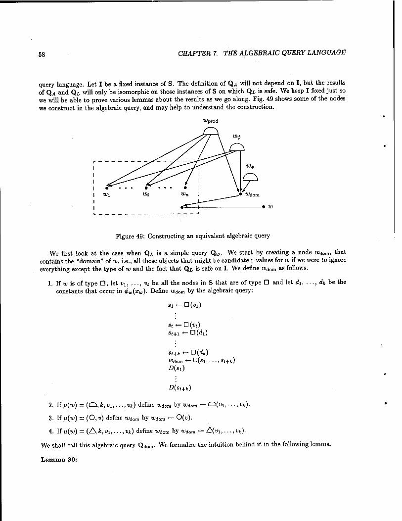
58 CHAPTER 7. THE ALGEBRAIC QUERY LANGUAGE
query language. Let I be a fixed instance of S. The definition of QA will not depend on I, but the results of QA and QL will only be isomorphic on those instances of S on which QL is safe. We keep I fixed just so we will be able to prove various lemmas about the results as we go along. Fig. 49 shows some of the nodes we construct in the algebraic query, and may help to understand the construction.
Wprod
• W
Figure 49: Constructing an equivalent algebraic query
We first look at the case when Qi is a simple query Q«,. We start by creating a node u>dom, that contains the "domain" of w, i.e., all those objects that might be candidate r-values for w if we were to ignore everything except the type of w and the fact that Qx, is safe on I. We define lUdom as follows.
1. If w is of type D, let vi, ..., vt be all the nodes in S that are of type D and let di, ..., dk be the constants that occur in <f>w(xw). Define tUdom by the algebraic query:
si<-D(vi)
st «-D(ui) st+i«-D(di)
st+k <-~D(dk) tUdom <—U(s1,...,Sj+ifc)
£>(Sl)
D(st+k)
2. If p(w) = (C2i,k,vi,...,Vk) define tudom by u>dom *- <^(v\,.. .,vk).
3. If p(w) = (O, v) define wd0m by tudom <- O(u).
4. If fj,(w) = (£s,k,vi,...,Vk) define wdom by wdom <— Z^i,.. .,«*)•
We shall call this algebraic query Qdom- We formalize the intuition behind it in the following lemma.
Lemma 30:

7.2. EQUIVALENCE OF THE LOGICAL AND ALGEBRAIC QUERY LANGUAGES 59
1. The schema created by Qdom is equal to the schema of S together with a node u>dom of the same type and with the same children as the node w in the original logical query Q„,.
2. Let Idom be the result of Qdom on I and let I„, be the result of Q„, on I. If r is an r-value in Iw(tu), then r is also an r-value in Idom(«>dom)-
Proof: If w is of type O, A or O, the lemma is obvious. If w is of type D, the first part follows from the fact that all the nodes except wdom that are created by Qdom are also deleted by it. The second part is an immediate consequence of Lemma 24 (page 43) and the definition of Qdom- I
We may assume, if necessary by renaming some bound variables, that all the bound variables in the formula <j>w{xw) that was used to define Q„, are distinct. Let these variables be zj, ,...,«* . The algebraic query Qprod on the result of Qdom consists of the algebraic operation
u>prod <- Q(iui, ...,wk,wdom)
For the purpose of defining QA we are going to label the edges with head tuprod as follows. The ith edge with head wprQd will be labeled x[,.. These labels will be used only to define the algebraic query, and are not themselves part of the query.
In certain cases, when we create a new node using some algebraic operation, the outgoing edges from the new node will inherit the labels of the corresponding edges whose head is one of the arguments of the operator. We shall only use this inheritance in cases when it is unambiguous, i.e., in cases when all the arguments have the same labeling. The operations for which labels will be inherited are aiSj, difference and union. When we use the projection operation the new edges will also inherit the labeling of the corresponding edges whose head is the argument of the projection. These labels are essentially used to remind us which bound variable the edge corresponds to.
Arrange all the well formed subformulas of <l>w(xw) in a list Vi, • •., Vw where Vm = <f>w(xw) and Vi precedes ty whenever it is a subformula of rpj. For each such subformula, we shall define an extended algebraic query Q^ on the result of Q^_,. Q^ will be a query on the result of Qprod. The labels on the edges with tail u^ will correspond to the variables that might be free in ip—i.e., those that haven't yet been bound by V- The node w+t will be of type ((=^,j,wjl,...,wjk,wdom), and will contain, intuitively, those tuples (/!,...,lk,ld) for which \=i^Mli, ■■-,h,ld)-
1. i>i is x%^ 9 xbWb. Q^j consists of the algebraic operation «ty. *- <ra g j(iüprod).
2. V» is x$,a 0 xw. Q,^ consists of the algebraic operation w^ <- aa8 *+i(tuProd)
3. V. is xw 9 xw. Q^,,. consists of the algebraic operation w^,i «- ah+1 9 *+i(u;prod)
4. Vi is x^a =r d. Q^ consists of the algebraic operation wj,. <- <Ta=rd(wProd)-
5. fa is xw =r d. Q^j consists of the algebraic operation w^. «- 0-(jfc+i)=rd(iUprod)
6. i>t is iph V V>3. Let Ai be the (ordered multiset of edges with tail w^ that have the same label as some edge with tail w^. Let A2 be the corresponding set of edges with tail w^ . Q^{ is the following extended algebraic query J3
«i *-nj4l(ti^ii) S2 «-IW«^) uty, <-U(si,s2) D(Sl) D(s2)

60 CHAPTER 7. THE ALGEBRAIC QUERY LANGUAGE
(si and s2 are different temporary nodes from those used above, and from similarly named nodes used below.) Note that the way we defined Ax and A2 guarantees that there is no ambiguity in labeling the edges of the result, at least as long as the labels of the edges in Ai and A2 are in the same order. We shall show later that this is indeed the case.
7. V. is -<il>j- Let A be the (ordered multiset of edges with tail wdom that have the same label as some edge with tail w^. Q^ is the following extended algebraic query
«I «- IU(utydom) Wipi <— «i — Utyj D(Sl)
As in the previous case we shall be able to label the edges with tail w^ without any ambiguity.
8. xßi is (3x1 )(V>>). Let A be the (ordered multiset of all edges with tail w^ except for the edge labeled xwa • We'shall show later that there must be exactly one edge with such a label. Q^. then consists of the algebraic operation uty{ <— n^iu,^).
Lemma 31: Let V = 1>i be one of these well formed subformulas of <t>w(xw). Let x^, ..., x% be those variables in the above list that are not bound in &. Note that some of the asj^'s may not actually occur in
rPi. Then tu*, is of type (Q, (a, + 1), wttl, ■ ■ ■, waj,wdom), and the tth edge with tail w+t has head to«, and is labeled with the variable «J«. As a consequence of this, all the labelings of edges are in the same order and the assumptions that we made on the labelings when we defined the u^.'s hold.
Proof: The proof is a fairly straightforward induction using the definition of w^. The tricky case is when V>i is Vji V Vi3- Then the children of w^ correspond to the bound variables of <f>w that are not bound in i>h and'the children of u^A to the bound variables of <f>w not bound in V>;3- Since a variable is not bound in V>ji V V>>3 iff it is not boundm ipjl and it is not bound in i>h, we see that the result does hold in this case. |
Lemma 32: Let to* be of type (Q, j,wh,. . .,tz^,u>dom)- Let 1^ be the result of Q^ on I, let ld be a member of V(tfldom) and let lt be a member of I*(uy.) for t = 1, ..., k. Then there exists an / in /*(»*,) with r(i) = ih,...,h,ld) if and only if \=^Mh, ■ ■ -,k,ld)- Intuitively, (h,...,lk,ld) is a "candidate
r-value" iff it satisfies ^i •
Proof: A straightforward induction on the structure of V>i- I The extended algebraic query Qfinai on the result of Q^«, consists of the following operations
D(W4,)
-D(Wprod)
■D(lOdom)
We finally define the algebraic query Qyi as
Qfinai ° Q* ° Q^m-i ° Qv>i ° Qprod ° Qdom
Lemma 33: Let i! be the result of Qw on I and let I2 the result of the algebraic query Q,i on I. Then Ix
and I2 are isomorphic relative to S.

7.2. EQUIVALENCE OF THE LOGICAL AND ALGEBRAIC QUERY LANGUAGES 61
Proof: First note that the Schemas are equal. The only node created but not deleted by Q^ is the node wA. This node is similar to the node tOdom and hence to w.
We have to show that the instances of wA and w are isomorphic, i.e., that at the point in evaluating the queries that we compute the instances of these nodes, they have the same candidate r-values. We assume that we are at the point in the evaluation of QA just before the final round of deletions.
Let r be a candidate r-value for w. Extend I to an instance I„, of SQ^ by defining Iw(w) = {/} and
r(l) = r. Then hl„<M0- Let ^ be the result of Q^„ on I. By Lemma 30 part 2, r is a candidate r-value for wdom and so for some ld in ^„(tUdom), r(ld) = r. By Lemma 18 (page 41), hlwM0 implies ^I^twild), and therefore, by Lemma 32, for some 1$ in I^{wdom), r(/^) = r is a candidate r-value for wA.
For the converse, suppose that r is a candidate r-value for wA. Let 1^ be the result of Q^ on I. Since r is a candidate r-value for wA, for some /^ in I*w{w+W) and some ld in I«J(iudom), r(^) = (/d)~and r(ld) = r. Since /^ is in /*„(«;*„,), Lemma 30 implies that |=i^u, (/«*). Restrict I^„ to an instance Ljom of the schema
of Qdom- Then l=Idom<£«;(*<*), and so by Lemma 18, r(ld) = r is a candidate r-value for w. |
We can easily extend this to general queries by concatenating the algebraic queries for the individual simple queries. If we have an extended logical query we have to add deletion operations at the end of the algebraic query that delete those nodes in the delete set of the query. This completes the proof of the following theorem.
Theorem 34: The extended algebraic query language and the extended logical query language are equiv- alent, i.e., for every extended algebraic query on S there exists a safe extended logical query on S and for every extended logical query on S there exists an extended algebraic query on S, such that both queries define the same schema and for every database instance I on which the logical query is safe, the results of both queries are isomorphic relative to S. |
Example 21: We shall illustrate the proof of Theorem 34 by showing how it would construct an extended algebraic query equivalent to the query Qi in Example 12 (page 37). We shall name the new node in that query t rather than u'. The database instance is shown in Table 10 (page 11).
1- Qdom consists of the algebraic operations sx <— D(u), <dom «- U(si) followed by D(s{), the deletion of si. Note that the union of copies of all database nodes of type D becomes here the union of a single node. This is of course superfluous, but as we are illustrating the proof of the theorem, rather than showing how to compute the result efficiently, we include this operation. The final schema (after the deletion) and the instances of the nodes are shown in Fig. 50.
2. Qprod consists of the operation <prod «- O(u,fdom). Fig. 51 shows the schema after this operation. The instance is too large to show here. It contains 25 1-values, 25-49, with all the possible pairs in {1,..., 5} x {20,..., 24} as r-values.
3. The subformulas of <j> are Vi = {xt =r yu) and <f> = ip2 = (3yu)(xt =r yu). Qv,1 is fy, «- o-2=ri(u>prod), and its result is shown in Fig. 52.
4. Q^ is ttf, <— II{tdom}(^1). Its result is shown in Fig. 53.
5. Qfinai consists of the operation tA <— 0m(<dom, fy) followed by the deletion of all the temporary nodes. The result of this is shown in Fig. 54.
This example shows that the algebraic query that we get from the proof, as is also the case in Codd's proof of the equivalence of the relational algebra and tuple calculus, is not necessarily the best way to actually evaluate a logical query. Our example could be done much more efficiently by the single algebraic operation tA «-O(u).

62 CHAPTER 7. THE ALGEBRAIC QUERY LANGUAGE
*dom I I
J(«l) I (t dorn)
I r(l) 15 Rehoboam 16 Solomon 17 David 18 Batsheba 19 Jesse
/ r(0 20 Rehoboam 21 Solomon 22 David 23 Batsheba 24 Jesse
Figure 50: Result of Qdom
<do
Figure 51: Schema of Qprod
7.3. Various Results about the Algebra
Most of the algebraic operators are natural analogues of relational operators. Even the powerset operator 0(v) is fairly natural, since it creates the entire domain of the node, and is therefore similar to the operator 0(t>i,..., v„) that is based on the cross product. The exception is the restriction operator, <Tin(u, v). Even though it is a type of selection, there is an essential difference between it and the other LDM selection operator. Restriction selects objects based on whether they are used in some other node, whereas the other selection operator selects objects based only on some property of the object by itself. For this reason, the LDM selection operator-resembles the relational selection while restriction does not.
For this reason, it would be nice if we were able to eliminate the restriction operator from the algebra, i.e., to show that it can be expressed in terms of the other algebraic operators. We now show that this is impossible.
Theorem 35: The extended algebraic query language is strictly more powerful than the language without restriction.
Proof: Let the database schema consist of the nodes u and v in Fig. 55. We claim that there is no extended algebraic query not using restriction that is equivalent to the query w *- ain(u,v). To see why this is true, note that the only algebraic operators apart from restriction that can create nodes of type D are the operators

7.3. VARIOUS RESULTS ABOUT THE ALGEBRA 63
Mom
/(**)
/ r(l) 50 (1,20) 51 (2,21) 52 (3,22) 53 (4,23) 54 (5,24)
Figure 52: Result of Q^
1. t*-n(vi)
2. t*-D(d)
3. t *-\J(vlt...,vn)
4. t *— V\ — V2
and in all these cases the arguments must also be of type D. Intuitively, the query must therefore construct the node w without looking at the node v at all. More formally, suppose that there existed an extended algebraic query Q equivalent to w <- <rin(u,u). Let Ii and I2 be the following database instances. Both h(u) and I2{u) are equal to {1,2}, where n(l) = r2(l) = a and rj(2) = r2(2) = 6. On the other hand, h(v) = h(v) = {3} but ri(3) = (1) and r2(3) = (2). The candidate r-values for w on these instances should be, respectively, a and 6. We shall show, by induction on the length of Q, that for any node t in Q of type D, in particular w, the candidate r-values for t on both Ix and I2 are the same. For Q of length 0, the result is obvious. Assume that the inductive hypothesis holds for all queries of length less than n, and let Q be of length n. If the last operation in Q is a deletion or if the last operation creates a node of type other than D, the result is immediate. If the last operation creates a node of type □, it must do so using one of the operations 1-4 above, and then the result follows immediately from the inductive assumption. |
Our second result shows that the extended algebraic query language is strictly more powerful than the nonextended logical query language.
Theorem 36: There is an extended algebraic query that is not equivalent to any (nonextended) logical query.
Proof: We shall show that there is an extended logical query not equivalent to any (nonextended) logical query. The result will then follow by Theorem 34.
The database schema S will be the same as the one we used in the proof of Theorem 26 (page 44). The extended query Q will also be the same as in that proof, together with the set of temporary nodes {u, w}.

64 CHAPTER 7. THE ALGEBRAIC QUERY LANGVAGE
U\J
I(tA) Figure 53: Result of Q^
nu) i r(0
55 (20) 56 (21) 57 (22) 58 (23) 59 (24)
/ r(l)
60 Rehoboam 61 Solomon 62 David 63 Batsheba 64 Jesse
Figure 54: Result of Qfinai
An equivalent logical query would have to define the contents of t in terms of the contents of v alone, which we showed in the proof of Theorem 26 to be impossible. |

7.3. VARIOUS RESULTS ABOUT THE ALGEBRA 65
D
Figure 55: Proof that restriction is essential

Chapter 8
Elimination of Cycles
8.1. Introduction LDM schemas can contain cycles not only in the Schemas but also in the data. For example, if / e r(/) for some 1-value /, then we would have a cycle in the data. Having introduced cycles into the model, we would like to study their expressive power. The problem we shall look at is: Are there applications that cannot be modeled without cycles? For example, consider the following schema.
Example 22: Fig. 56 shows an example of a cyclic database schema that stores information about procedure calls in a program. The schema is the same as the genealogy schema that we have used up to now. Elements in I(v) represent procedures, elements in I(u) represent procedure names and elements in I(w) represent sets of procedures. Thus, if x € I(v) and r(x) = (y, z), then r(y) is the name of the procedure x and r(z) is the set of procedures called from x. Note that if a procedure calls itself, then we have a cycle in the data. This is the reason we do not use the genealogy example, since the data in the genealogy should not be cyclic. An acyclic schema that intuitively seems to "capture the same information" is shown in Fig. 57. In this schema, elements in I(v2) represent procedure entities, elements in I(u) represent procedure names, elements in I(w) represent sets of procedures, and elements in I(vi) represent the relationship "procedure calls procedures."
To formalize the idea of "capturing the same information," we use a definition, closely related to the notion of query-equivalence of [Hul84]. Intuitively, two schemas capture the same information if we can map instances of one schema to instances of the other, and queries on one schema to queries on the other, such that the result of the first query on the first instance is isomorphic to the result of the second query on the second instance.
In our query language, however, the result of a query is not necessarily a new, independent schema, but may contain pointers to nodes in the database schema S. Because of this, it is meaningless to talk in general about isomorphism between the results of the queries. In order for such an isomorphism to be meaningful we shall restrict the query language, in this chapter, to a language that does not allow pointers to the database.
Definition 35: A independent query on a schema S consists of a new schema SQ together with an ordering of nodes and a set of LDM formulas, such that when we add the query schema to the database schema we get an LDM query.
The result of an independent query is defined in the obvious way. If two independent queries on different database schemas have the same query schema, we are then able to talk about their results being isomorphic.
66

8.2. CONVERTING CYCLIC SCHEMAS TO ACYCLIC ONES 67
1Ü
Figure 56: Cyclic schema Figure 57: An acyclic schema equivalent to it
Definition 36: Let S and T be Schemas. Then T dominates S if there is a mapping / of instances of S to instances of T such that for each independent query Qx on S, there is an independent query Q2 on T such that Qi(I) is isomorphic to Q2(/(I)) for all instances I of S on which Qi is safe. We say that S and T are equivalent if each of them dominates the other.
We shall only be able to prove that the two Schemas in Example 22 are equivalent when the relationship represented by vx is functional, i.e., when for each procedure is related to exactly one set of procedures, i.e. those procedures that it calls. This means that in fact we do not have an equivalence between the Schemas, but rather between the original schema and a new, constrained one. To make our results more general, we shall also start off with a constrained schema, so that we shall in fact show an equivalence between a constrained schema (S,<f>) and an acyclic constrained schema (T,rp). We start by describing the general transformation from cyclic Schemas to equivalent acyclic Schemas. The idea is to break cycles by creating composition nodes that represent the cyclic relationships, as in the above example.
8.2. Converting Cyclic Schemas to Acyclic Ones
When we try to break cycles in arbitrary cyclic Schemas, we notice that there are several pathological cases in which the above method does not work. First of all, the cycle has to contain a O or Anode at which to break it, i.e., it cannot consist just of O-nodes. The method also fails when the cycle contains such a node of type O or A, but this node has only one child. If we break the cycle at such a node, we would end up with a childless O or Anode after breaking the cycle. In both of these cases, the schema relates 1-values to 1-values without relating them at any point to the actual data. Intuitively, pure relationships between 1-values such as these do not correspond to anything in the "real world," which justifies looking only at schemas without such a relationship.
We make one further restriction on the LDM schemas. If a cycle in the schema contains a node of type A our method of removing cycles appears not to work. For example, if the cyclic schema was the one shown in Fig. 58, it would be converted into the schema in Fig. 59, that does not represent the same structure. The original schema essentially stores data objects at the top node, along with sets of objects, sets of sets of

68 CHAPTER 8. ELIMINATION OF CYCLES
objects, etc, and this is not what is stored in the acyclic schema. For this reason, we shall require that nodes of type Aoccur only outside cycles. Unlike the other conditions, this is a real restriction on the power of our method, and more work remains to be done on whether cycles involving nodes of type A can be eliminated.
Figure 58: A cyclic schema Figure 59: Corresponding acyclic schema
Definition 37: A schema S is called well-formed if from each node in the schema there is a path to a node of type D, and no node of type A occurs in any cycle of S.
Definition 38: Let S be a cyclic schema. A node v in S is called a possible breakpoint if
1. It is of type O.
2. It is in at least one cycle.
3. It has at least one child that is not in any cycle.
For example, the node v in Fig. 60 is a possible breakpoint.
Lemma 37: Let S be a well-formed schema. Either S is cyclic, or it has a possible breakpoint.
Proof: Assume that S contains a cycle, and let u0 be a node in that cycle. Since S is well-formed, there is a path uo, ..., u« from u0 to a node un of type D. Let uk be the first node on this path that is not in any cycle; there must be at least one such node, since the node un is not in any cycle. We claim that the node ujt-i'is a possible breakpoint. By definition, it is on at least one cycle and has a child that is not in any cycle. Since uk-\ is in a cycle and that cycle does not contain uk, ut-i must have at least one other child. Since S is well-formed, uk-i must be of type O. |
Let S be a well-formed cyclic schema, and let v be a possible breakpoint. There are two ways to generalize Example 22. One way is to break one cycle through v at a time. In some cases this can result in unnecessarily complicated Schemas, and we prefer instead to break the cycles that go through v all at once. The node v is replaced by two nodes Vl and v2 (see Fig. 61). All the edges that had head v, except for those that belonged to one of the cycles through v, will now have head vi. All the edges that had tail v, except for those that were in the cycles, now have tail v2. «i and v2 will both be of type Q. The formal definition is as follows.
Definition 39: Let (S,<f>) be a well-formed cyclic constrained schema, where S = (V,E,p), and let v be a possible breakpoint. Then Br(S,^,v) is the constrained schema (S',V) where S' = {V',E',(i') and
V> = Br((^, v) are defined as follows.

8.2. CONVERTING CYCLIC SCHEMAS TO ACYCLIC ONES 69
y
o ™3 Wrn «„ U3
/* ^
W2
r .....
—••*
• «2
-•- "1
IÜ1 •
yf~\
Figure 60: Cycles through v Figure 61: After breaking the cycles
_ {( u {( u {( u {( u {( u {(
1. We introduce two new nodes vx and v2. V has v replaced by vx and v2, i.e., V = V - {v} U {«i, v2}.
2. All the nodes in V except for vx and v2 have the same type as in S, i.e., fi'(u) = ß(u) for all u in V — {v}. vi and v2 are both of type O.
3. Let C be the set of nodes that are on the cycles that go through v. Then E' is defined as follows
E' = E - i(ui,u2) | (ui,u2) £E,ui = v or u2 = v] («1,^2)} (u,«i) |(«,u) G£^,u^C7} (u, D2) j (M, V) e E,ueC} (v2,u) \{v,u)£E,u£C} (v1,u)\(v,u)eE,ueC}
In other words, the edges in the new schema are
(a) All those in the original schema, except for those whose head or tail is v. (b) v2 is a child of v\.
(c) Each edge with head v is replaced by
i. An edge with head vi, when the edge is not part of a cycle. ii. An edge with head v2, when the edge is part of a cycle.
(d) Each edge with tail v is replaced by
i. An edge with tail w1( when the edge is part of a cycle. ii. An edge with tail v2, when the edge is not part of a cycle.
Any edge that replaces an edge with head or tail v has the same position in the ordering as the edge it replaces. The edge from ui to v2 follows all the other edges in the ordering.

70 CHAPTER 8. ELIMINATION OF CYCLES
In order to define the new constraint ip = Bi(<j>,v), we first define a function F(<j>) from LDM formulas over S to LDM formulas over S'.
Definition 40: The function F(<j>) is defined by induction on the size of <f> as follows.
1. (a) If u and w are not equal to v, then F(xu x„ yw) is xu xu Vw
(b) If w is not equal to v, then
i. If w is not on a cycle through v, then F(xv x„ yw) is aj„1 x„ yw. ii. If tu is on a cycle through v, then F(xv x„ yw) is xV3 x„ yw.
(c) If u is not equal to v, then
i. If u is not on a cycle through v, then F(xu x„ yv) is xu xu yV2. ii. If w is on a cycle through v, then F(xu xu yv) is xu x„ j/Wl.
(d) F(xv xt y„) is s„3 x„3 j/^.
2. .F(a:„ G y«,) is defined similarly, except that we do not have to worry about the cases when w = v.
3. F(xu p yw) is similar to the previous case.
4. (a) If u is not equal to v, then i^s« =; yu) is xu =/ j/u.
(b) F(xv =/ j/„) is xVl =i yVl.
5. ^(a;« =r d) is x„ =r d.
6. F{<f>Ai>) is F(4) A F(j>).
7. (a) If u is not equal to v, then F((Va;u)^) is (Vzu)F(<£).
(b) F((Vxv)<l>) is (VajCl)(Va;0:i)((a!0a x„3 xUl) A F(<f>)), where a;^ and a;„3 are new variables, and the projection uses the last edge from V\ to V2 ■
Definition 41: The constraint <f> is mapped into the constraint
Br((£,») = F(4>) A (VxSJiVxlJiVxvJixu, x„3 xa
Vl A xV3 x„3 as*1 =*■ xani =, xb
Vl) A {WxV3)(3xVl)(xV3 x„3 xVl)
The last two conjuncts express the functional relationship that exactly one D2 is associated with each vi.
Lemma 38: Let (S, <f>) be a well-formed cyclic schema, and let v be a possible breakpoint. Then Br(S, <j>, v) = (S', ip) is also well-formed.
Proof: We first have to show that S' is a legal LDM schema. The only reason it may fail to be one is that S' may contain a node of type O that has no children. It is clear from the definition of S' that the only node where this could happen is V2, but V2 has at least one child since v has at least one child that is not in any cycle through v.
We now show that S' is well formed. Let w be an arbitrary node of S'. We have to show that there is a path in S' from w to a node of type D, and that no cycle contains a node of type A To prove the second of these, it is not hard to show that we can convert a cycle in S' into a cycle in S by replacing all occurrences of vi and v2 in the cycle by the node v. For the first condition there are two cases.
1. w is neither of the nodes vi and v2. Then w must be a node of S. Since S is well-formed, there must be a path in S from tu to a node x of type D. Let w, tui, ..., wn, x be a shortest such path. Clearly x is also in S'. If all the other nodes on the path are also in S', we are done. Otherwise, one of these nodes, say w,, is equal to v, and by the minimality of the path there is at most one such W{. Since v is a possible breakpoint, it has a child «i that is not on any cycle, and therefore there is a path ui, ..., um in S from «i to a node um of type D (see Fig. 62). There are then two possibilities.

8.2. CONVERTING CYCLIC SCHEMAS TO ACYCLIC ONES 71
• w
• Wi-l
• to, = V
• •
Figure 62: Proof of Lemma 38
(a) Wi-i is not on any cycle through v. Then w, ..., Wi_lt vu v2, ux, ..., um is a path in S' from w to a node um of type D.
(b) u)j_i is on a cycle through v. Then io, ..., tu<_i, »2,«i «misa path in S' from tu to a node um of type D.
2. w is either «,. or v2. If we have a path from v2 to a node x of type D, we can easily convert it to a path from vi to z by using the edge (vuv2). Assume therefore that w is the node v2. Since v is a possible breakpoint, it has a child wi that is not in any cycle. Since S is well-formed, there is a path from w1
to a node x of type D. Let wlt ..., wn, x be the shortest such path in S. Then no node on this path is equal to v and therefore v2, u>1; ..., wn, x is a path in S' to a node x of type D. |
We now show that if we repeatedly break cycles, we eventually get an acyclic schema.
Lemma 39: Let (S,<£) be a well-formed constrained cyclic schema. If we repeatedly break cycles in S at possible breakpoints, we shall eventually get an acyclic constrained schema (T,V). The termination does not depend on the order in which we choose the breakpoints.
Proof: The proof is by induction on the number of nodes of the schema that are in at least one cycle. We show that whenever we break a cycle we reduce the number of such nodes by at least one. Let (Si,^) be the schema before breaking the cycles through v and let (S2,<fo) = Br(S1,(^1, v) be the schema afterwards. We show that
1. The two new nodes vx and v2 are not in any cycle in S2.
2. Any node in Si other than v that is not in any cycle in Slt is also not in any cycle of S2.
Together, these conditions immediately imply the result.
1. Assume that there is a cycle in S2 that goes through vx or through v2. Let C be the shortest such cycle. There are three cases
(a) C contains vi but not v2. Let w be the node in C that immediately precedes vx. By replacing vi in C by v we get a cycle in Si. But then, when we construct S2, we replace the edge (w,v) by the edge (w, v2), and S2 then contains no edge from w to vx.

72 CHAPTERS. ELIMINATION OF CYCLES
(b) C contains v2 but not vu Let u be the node in C that immediately succeeds v2. In a similar way, by replacing v2 by u, we get a cycle in Sx. Therefore, when constructing S2, we replace the edge (v, u) by the edge (t>i, u), and S2 does not contain an edge from v2 to u.
(c) C contains both vi and u2. v2 must occur immediately after «i on C, since otherwise we could shorten the cycle C by replacing the path from t>i to v2 by the edge (vuv2). Let u be the node in C that immediately precedes vx. If we replace «i and v2 in C by the node w, we get a cycle in Si. But then the edge (u,«i) would be replaced in S2 by the edge («,«3) and S2 would not contain an edge from u to v2, a contradiction.
2. Let u be a node of Si that does not appear in any cycle, and assume that w is in some cycle C in S2. As we have just shown, no cycle in S2, and in particular C, can contain either of the nodes «i or v2. But then C is also a cycle in Si, a contradiction. |
8.3. Equivalence of the Schemas
We first show how to map an instance of (S, 4) into an instance Br(I, v) of (T, V) = Br(S, <f>, v). The intuition behind the construction is as follows. We got from S to T by breaking cycles through v. The instance of any node other than v, that does not have v as either a parent or a child, is not changed. Each 1-value in I(v) is replaced by a pair of 1-values, one in Br(I,t;)(t>i) and the other in Br(I,w)(ü2). The second of these 1-values is the child of the first. We then modify the r-values of the 1-values in the parents and children of v
in a straightforward way.
Definition 42: Let (S, <j>) be a well-formed, cyclic, constrained schema, and let Ii = (h, n) be an instance of it. Let v be a possible breakpoint, and let (T, V) = Br(S, *,«). Then I2 = (/2,r2) = Br(Ii,u) is the instance of T that is defined as follows. For each I in h(v), we introduce two new 1-values, that will be
written as a(l) and ß(l).
1. I2(Vl) is defined as {<*(/) | I G h{v)} and I2(v2) as {/?(/) | / 6 h(v)}, i.e., they contain all these new 1-values. Since 1; is of type O, for each such f in h(v), n(f) = (Jlf ...,/„) for some lu ..., /„. Assume, w 1 o g that the first i children of v are those that are in cycles through v. Then r2(a{l)) is defined as
(Ji, • • •, h, 0(0) and r*W)) a8 (;'+i • • • • • '»)• If the jth chiW °f V is V itS6lf' thCn thC corresP°ndin6 component of r2(a(l)) will be ß(lj) instead of (,.
2. If w is any node except v that is not a parent of v, then I2(w) = h{w), and for each I in this set,
r2(l) = r1(l).
3. If to is a node (except v) that is a parent of v, then 72(«;) is defined as h(w). For the r-values, there
are two cases to consider.
(a) w is not in any cycle that goes through v. If w is of type (Q,n), then for each J in h(w), rM) = (k,...,/„) for suitable /;'s. Let v be the ith child of w Then r2(/) is defined as (li,..., Zj_i,'a(ii). h+i, ■ ..,/«)• This generalizes easily to the case when there multiple edges from w to 'v. The other possibility is that w is of type (0,v). In that case, for each / in I2(w), r2(l) is
defined as {»(/') | /' € ri(l)}.
(b) w is on a cycle through v. The r-values are defined as in the previous case, but with ß{l) used
everywhere instead of a(/).
Lemma 40: Let I be an instance of (S, <j>) and let v be a possible breakpoint. Let I* be the instance Br(7, v).
Then I* is an instance of the schema (T, V>) = Br(S, <f>, v).
8.3. EQUIVALENCE OF THE SCHEMAS 73
Proof: We have to show that I* satisfies the constraint Bx(<f>,v). It is clear that it satisfies the two final conjuncts in the definition ofBi(<j>,v), since there is a 1-1 correspondence between 1-values a(l) in P(t>i) and 1-values /?(/) in I* («2). It remains to show that \=j.F(<f>). This is a consequence of the following assertion, whose proof is a routine induction on the structure of the formula <f>.
Let i){x]Ui,..., x^n, yl,..., y™) be an arbitrary LDM formula over S where all the variables of sort v are at the end. Then the free variables of Fty) are^ ^, y^, yl2, ..., y^, y™. It lt € I(Wi) for all *, 1 < 1 < n, and l[ G I(v) for i = 1, ..., m then
^im,---JnJ[,...J'm)^\=I.F^)(lu...Jn,a(l[),ß(l[),...,a(l'J,ß(l'm))M
Lemma 41: Let (S,<£) be a well-formed constrained cyclic schema, let v be a possible breakpoint, and let (T, V>) be the schema that we get by breaking the cycles that go through v. Then (T, V>) dominates (S, <j>).
Proof: Let Qx be an independent query on S. Q2 will consist of the same schema as Qi and its nodes will be in the same order. Each formula <f>w(xw) in Qj is replaced by the corresponding formula F(</>w)(xw) in Q2. It is clear that we get a logical query.
Let I be a fixed instance of (S, <j>) and let P be the instance Br(I, v) of (T, V>). We show that the result Ii of Qi on I and the result 1\ of Q2 on I* are isomorphic. The isomorphism is defined using the topological order on the query nodes, as follows.
Assume that we have defined the isomorphism / between Ij and 1\ on all the query nodes that precede the node u. For each / G Ix(u), let r = n(/) be its r-value. We define an r-value r' as follows
1. If v is of type Q, then r is a tuple (lu ..., /„). We define r' to be the tuple (f(k),.. ./(/„)).
2. If v is of type O, then r is a set, and we define r' to be the set {/(/) 11G r}.
3. If v is of type A then r = 7, and we define r' to be /(/).
4. If v is of type D, then r £ D, and we define r' to be equal to r.
It is straightforward to show that r' is a candidate r-value for u in Q2. This gives us a 1-1 correspondence between the r-values of h{u) and those of I{{u). If we then define /(/) = /*, where I* is the 1-value in 7J(u) with r-value r', we extend the isomorphism / to u. By repeating this for each query node u, we get an isomorphism between Ix and I\. |
We now define the inverse mapping on instances.
Definition 43: Let (S,<£) and (T,V>) be as above, and let I2 be an instance of (T,^). Then Ii is the following instance
1. h(v) is defined as 72(ui). Whenever / G h(v), n(l) will be a tuple containing all the components from r2(/), except for the last one that corresponds to the new edge to v2, together with all the components ofr2(II„2(0).
2. If w is any node except vi and v2 and w is not a parent of v2, then Ii(w) = I2(w) and the r-values are the same as in I2.
3. If w is any node except vi that is not a parent of v2 then I^w) = I2(w). If w is of type (O, n) with v2
as its kth child, then each / in I2{w) has an r-value of the form r2(l) = (lu.. .,lk,.. .,ln) for suitable /,'s. Since I2 satisfies xj), there is a unique l*k in I2{vi) with lk as its last component. We then define i~i{l) = (h,..., 11,..., /„). We define the r-values for nodes of type O in a similar way.
Lemma 42: Let (S, <j>), (T, tp), I2 and ^ be as in the above definition. Then Iy is an instance of (S,<£).

74 CHAPTERS. ELIMINATION OF CYCLES
Proof: Ii clearly is an instance of S. The proof that ^^ is a straightforward induction on the structure
of <j>, similar to the proof of Lemma 40. I It is easy to show that the two mappings on instances are inverses of each other, i.e., applying one and
then the other yields an instance isomorphic to the original one. To complete the proof of equivalence we
show that (S,<j>) dominates (T,V>)-
Lemma 43: Let (S,<f>) be a well-formed constrained cyclic schema, let v be a possible breakpoint and let (T, VO be the schema that we get by breaking the cycles that go through v. Then (S, <f>) dominates (T, i>).
Proof: Let Q2 be an independent query on S. Qi consists of the same schema and node ordering as Q2. The formula <l>w(xw) in Q2 is replaced in Qi by the following formula. Each variable in <j>w of the form xVl
or xV3 is replaced by a variable xv. These variables are distinct, i.e., xVl and xVa are replaced by different variables. The only other change we have to make in <t>w is to atomic formulas that involve x*. Formulas of the form yw x,- xVl and yw x; xVa are replaced by yw x* xv, where w is the kth child of v. The remaining possibility, xVl x„+i y„3, where v has n children, is replaced by xv =j yv. Proving the equivalence of Qi and Q2 is now straightforward, making use of the fact that we only consider instances that satisfy the constraint
Combining Lemmas 41 and 43, we get
Lemma 44: Let (S,<f>) be a well-formed constrained cyclic schema, let v be a possible breakpoint and let (T, V>) be the schema we get by breaking the cycles that go through v. Then (S, <f>) and (T, V>) are equivalent.
Finally, by applying this result repeatedly together with Lemma 39, we get the desired result.
Theorem 45: Let (S,c£) be a well-formed constrained schema. There exists an acyclic constrained schema (T, V") that is equivalent to (S, <f>), I

Chapter 9
Conclusions
We have described a new model of data, the Logical Data Model, that is designed to combine the advantages of the existing data models. On the one hand, it enables the database to describe more of the semantics of the data than is possible using the relational model of data. On the other hand, we do not lose the nice properties that relational databases have, in particular the ability to query the database using equivalent non-procedural and procedural languages.
Some directions for future work are as follows.
1. More work has to be done on the query language. The languages we have defined are similar to the initial versions of Codd's relational algebra and tuple calculus. We have outlined in Section 3.2 how the LDM languages could be modified to obtain a more user-friendly and efficient language, but more work has to be done in this direction before an implementation would be possible.
2. Another direction for future work is extending the power of the query language. While there does not appear to be any need for the full power of the implicitly defined queries in our first attempt, there may be specific constraints that we want the result of the query to satisfy, and these may not be expressible by node-by-node formulas. Appendix B gives one example of the sort of difficulties we encounter in one extension of this sort.
3. The query languages that we have described are all first-order. Recent papers, such as [HN84] [Rei78] [U1185], have proposed using a more powerful query language, similar to PROLOG, for accessing databases. Such a language would be able, among other things to compute the transitive closure of a relation, something that cannot be done in the relational algebra [AU79]. It may be possible to extend the LDM query language along these lines to get a non first-order language without the problems that arise with Jacobs' database logic.
4. More work remains to be done on the expressive power of cyclicity. It is still open whether cycles containing nodes of type A can be eliminated. Furthermore, we have only shown that, according to a certain measure, cycles in well-formed Schemas do not add any expressive power. But it is not clear that this measure is the ultimate one.
75

Appendix A
An Early Attempt to Define the Query Language
A.l. Introduction In this appendix, S will be a fixed database schema, I an instance of it and Q = (SQ, XQ, <£Q) a query on
S. One of our attempts to extend the relational model to LDM schemas was the following. A query consists
of an extension of S together with some sentence that specifies an instance of it. In other words
Definition 44: A query Q on S consists of
1. An extension SQ of S.
2. An LDM sentence <£Q over SQ.
The result of the query should be an extension of I that satisfies sentence <f>Q.
Definition 45: The result of Q on I is an extension IQ of I to SQ such that (=j 4>Q.
One problem with this definition is that there may be many different ways to extend I, all of which satisfy <f>Q. One way we tried to deal with this problem was to require that a query have a unique result, i.e., put the burden on the user to make sure that he only asks such queries. Uniqueness, of course, will only be up to isomorphism. In the relational model the term safe queries is used to denote queries for which the result is defined. The only thing that could go wrong there is that the result may be infinite, and that is in fact the definition of safety in the relational model. For LDM queries this is no longer true, since there are other things that may be wrong with a query. For example, there may be no extension of I to SQ that satisfies the query, or there may be several possible such extensions. We shall borrow the term safe query from the relational'model and use it with an extended meaning. It will denote those queries that have a unique result. Note that since we are only interested in finite instances the safe queries in the relational model turn out to be a special case of our more general definition.
Definition 46: A query is safe up to isomorphism if for every instance I of S there is a unique extension of I to SQ that satisfies <J>Q. The uniqueness is up to isomorphism relative to S.
76

A.l. INTRODUCTION 77
The problem with this definition is that requiring that a query be safe up to isomorphism is too strong a requirement.
w*
Figure 63: A logical query
Example 23: Let the database schema be the genealogy schema S shown in Fig. 8 (page 10) Suppose that as a query on S we want to construct the LDM schema that corresponds to the relational model. In other words, the query schema is the extension of S formed by adding the nodes in Figure 63 to S. We want w* to contain pairs of 1-values that correspond to (Person-Parent) pairs. To get these pairs, look at elements of I(v). For each such element, take its left component and pair it with those elements that we get by taking the elements in its right component, and finding the person that they point to. When we write this out formally, we get the following LDM sentence
*i = (V^.)(V^0(V^.)f(^.xu.^.)A(x3.x„.^.)
=> (3yl)(3yl)(3y3v)(3yt)(3yS)((yl =r *'.) A (yl =r x*.) A (y? =r (,£,»*))
A (y5vey4
w)A{ylTuy^\
We can think of <f>x as being similar to how we would express a query in the relational model. In other words, we say what the objects in the result should satisfy. The problem with this query is that it is not safe up to isomorphism. One reason for this is that unlike the relational model the LDM model can express duplication of data. Everything in the result of the above query does indeed correspond to a (Person- Parent) pair but there is nothing to stop such a pair from appearing twice or more often. To prevent this from happening, we have to add another sentence to the query. The following sentence, <j>2, says explicitly that the result contains no duplication.
<t>2 = (VZu.XVj/t.*)^«* fr yu. =>. Xu. ±r yu.) A (ViEu.XWo.Xav ^j y„. =>• JE„. ^r y„.) A (Vxw*)(Vyw)(xw- ±\ yw. => xw- ^r yw,)
The query with fa A <f>2 is still unsafe. Nothing in what we have written so far says that any particular (Person-Parent) pair must appear in the result—we have only said that everything in the result is such a pair and that nothing appears more than once. In the relational model this is something that we do not have to say explicitly—we just say what should be in the result and the result will then contain one copy of each tuple that satisfies the query. To make our query safe we can add another sentence, <j>3, to the query. fa says explicitly that anything in I that corresponds to a (Person-Parent) pair gives rise to a corresponding

78 APPENDIX A. AN EARLY ATTEMPT AT THE QUERY LANGUAGE
tuple in the result.
4>z = (Vyi)(Vy2)(V^)(V^)(Vy5) UfrulÜ) A (vt^vl) A (rf .€ J&) A (tf»x„|tf)
=> (3^.)(3^.)(3^)((4* =r (*«-*«•)) A (*2- =r !#) A (**. =r »*) J J
Finally, to get a safe query, we have to restrict the contents of I(u*) and I(v*), i.e, to say that these nodes contain nothing that is not needed for the tuples in I(w*). Formally
<f>A = (Vxu*)(lyw*)(xu*iru.yw-) A (Vxv.)(3yw.)(xv*Tv.yw*)
Putting all this together we get the query Q = (SQ, <£Q) where
^Q = ^i A <j>2 A <t>3 A ^4
While this query is safe at last, it is obviously far too complicated to be any real use.
A.2. Safety up to Duplication
What the above example shows is that to get a safe query we have to add conjuncts to our original query that say things that are obvious. One of these explicitly states the fact that there is no duplication in the result. We could simplify what the user has to write by making this part of the definition of the query language, which could be done by having the query processor automatically add a conjunct similar to <f>2 to the query. We feel that this is not the right way to proceed for several reasons. One reason is that this seems a rather ad hoc approach. Why add this conjunct rather than other ones? The other reason is that the query may, either implicitly or explicitly, require that there be some duplication in the result. If the system were then to add <j>2 to the query it would convert what was originally a safe query into an unsafe one.
The alternative way to proceed that seems preferable from a mathematical viewpoint as well is to keep the original query as the condition that the result must satisfy but also require that the result have as little duplication as possible. In our example this would mean that there is no duplication at all but in general that would not have to be the case. A safe query would then be one that has a unique minimal instance satisfying the query. In such a case we shall say the query is safe up to duplication.
Essentially, an instance is minimal if there is no smaller instance that satisfies the sentence. Some difficulty occurs when trying to define what minimality means at a node of type O. If v is of type (O, u) and the query requires that u have some duplication, we have to make sure that we minimize internal duplication in the sets, i.e., that we take only one copy among the duplicates in u as a member of each set in v (unless duplication of this sort is also required by the query).
In order to define minimality, we first define a relation h ■< l2 on 1-values. k X l2 will mean, intuitively, that while h and l2 contain the same information, h may contain more internal duplication than l2.
Definition 47: Let Ii = {h,rx) and I2 = {h,r2) be two extensions of I to SQ. We say that an element h
of h(v) is dominated by an element l2 of h{v), and write h -< l2, iff
1. If v is a node of the database schema S, then h = l2. This means that different 1-values in the database are regarded as essentially different objects, even if their r-values are the same.
2. If v is a query node, i.e., v is a node in VQ - V, then
A.3. ABSOLUTE SAFETY 79
(a) lfß(v) = D, then nft) = r2(/2).
(b) If ß(v) = (O, n), then ü:(/i) ^ n,(/2) for all *, 1 < » < n.
(c) If ß(v) = A then n(/!) ^ r2(/2).
(d) If ju(v) = O, then
i. There is a 1-1 function /„: nft) - r2(/2) such that for all / G i^ft), Z -< /(/), i.e., everything that is m ri(/i) is also in r2(/2), possibly with more internal duplication.
ii. For every / G r2(/2), there is an /' G n(h) such that /' < I, i.e., everything in r2(/2) is a copy, possibly with some more internal duplication, of something in ri(h).
Provided that the query does not add cycles to the database, this definition corresponds to the intuition we described above. The problem with cyclic queries is that since the definition is recursive, 1-values of nodes that are m a cycle added by the query will never dominate one another, and we shall end up with no way to compare the instances that we get. As we are going to forbid cycles in the query anyway, for other reasons we shall not discuss here how to modify the definitions to handle cyclic queries.
The next step is to define a relation Ix X I2 between instances. Intuitively, Ix < I2 will mean that Ii and I2 contain the same data, but I2 may have more duplication. This means that I2 may have more copies of things in Ii, and these copies may have more internal duplication.
Definition 48: Let Ix = (/1)Pl) and I2 = {/2,r2> be two extensions of I to SQ. We say that Ix X I2 iff for each query node v
1. There is a 1-1 function /„: h(v) - I2(v) such that for each / G h(v), I < /„(/), i.e., everything in Uv) is in l2(v), possibly with more internal duplication.
2. For every / G h(v), there is an /' G h(v) such that /' ^ /.
Definition 49: An extension IQ of I to SQ is called a minimal result of Q iff
1. IQ is a result of the query, i.e., (= j <^Q.
2. IQ is minimal, i.e., if 1^ is another extension of I to SQ such that I* -< IQ, but I* is not isomorphic to IQ relative to S, then IQ is not a result of Q, i.e., Jbj. ^Q.
Definition 50: A query Q is called safe up to duplication on I iff Q has a unique minimal result on I Q is safe up to duplication iff it is safe on all instances I of S.
Example 24: If we write the query of Example 23 as (SQ, fa A fc A fa) we get a somewhat simpler query, ihis query is safe up to duplication and has the desired result.
A.3. Absolute Safety
The other way to simplify the user queries is to enable the user to avoid having to specify fa explicitly fa just says that anything that is allowed (by fa) to be in the result actually appears in it. In other words what we want to do is to maximize the data in the result. We also want to combine this with minimizing the duplication as above. An absolutely safe query will be one that has a unique result under this combined approach, i.e., maximize data- and minimize duplication.
We first define what it means to say that an instance contains more data than another instance.

80 APPENDIX A. AN EARLY ATTEMPT AT THE QUERY LANGUAGE
Definition 51: Let Ix = (h,n) and I2 = (h,r2) be two extensions of I to SQ. We say that I2 contains at Jeast as much data as Ilt and write Ij < h, iff for each query node v and each element h <*h(v), there is an element l2 of I3(v) that contains the same information, possibly with more internal duplication, i.e.,
Definition 52: An extension IQ of I to SQ contains the maximum data satisfying Q iff
1. IQ is a result of Q, i.e., \=1 4>Q.
2. IQ is a maximum result, i.e., if IQ is an extension of I to SQ that satisfies hlj^Q. then VQ ^ *Q
Definition 53: The absoJute result of Q is an extension IQ of I to SQ such that IQ is minimal under ■<
in the class of maximum results, i.e., the class
{I* | l*Q contains the maximum data satisfying Q}
Definition 54: Q is absolutely safe on I iff it has a unique absolute result, up to isomorphism. Q is absolutely safe iff it is absolutely safe on all database instances.
Example 25: The query of Example 23 can be written as the absolutely safe query (SQ, 4>I A 4>A).
A.4. Undecidability What we have shown so far is how we can reduce the amount of work the user has to do in order to write a safe query The language we get is close in this respect to the relational tuple calculus. In order to do this, however, we had to make the definition of what the result of a query is much more complicated and less
intuitive. , . . Besides this, it turns out that all three of the approaches we described are too powerful. We look now
at the question how do we test if a given query is safe, either up to isomorphism, up to duplication or absolutely. It is not hard to see that we can reduce testing whether a query in the relational model is safe to testing safety under any of these definitions. Since testing a relational query for safety is undecidable fPao69l the undecidability of testing for our types of safety follows immediately. In the relational model his undecidability is not a problem. The reason for this is that if we are given a database instance we can test whether the query is safe and we can compute the result when it is. Furthermore, we can give restrictions on the query language that allow the user to write only safe queries, and if all the domains are finite then all relational queries are safe. What is undecidable is just to test whether a query is safe for all possible database instances. Our three definitions of safety, on the other hand, are too powerful, since even if we are given a database instance, it is still undecidable whether a query is safe on it.
Theorem 46: There is an acyclic schema S\ an instance I of S and a query Q on S, such that it is undecidable whether the query is safe on I up to isomorphism, up to duplication or absolutely.
Proof: We reduce testing the three kinds of safety to testing whether a sentence in a first-order theory with equality and one ternary relation symbol R(x, y, z) has a finite model [Tra50]. The database schema S will be the empty schema (V = 0), which immediately turns both testing for safety on a fixed instance, and on all instances, into the same problem. The query schema SQ is shown in Fig. 64. It has v <Q U.
iThe reason for mentioning the fact that it is acyclic is that otherwise the cyclicity of S might appear to be what causes the
undecidability

A.A. UNDECIDABILITY 81
u
Figure 64: Undecidable query
Let ^ be a sentence in the first-order theory. We convert this into an LDM sentence L(<j>) as follows.
1. Introduce a variable xv for each variable x in <f>.
2. Replace each quantifier Qx by Qxv.
3. Replace each atomic formula x = y in 4> by the LDM formula xv =, yv.
4. Replace each atomic formula R(x, y, z) by the LDM formula
4>R = (3wu)(wv =r (xv, yv, zv))
The query Q = (SQ, V>) has V equal to
L{4>) A (V«i)(V«»)(xi =r xl => xl =, xl) A (VylWylM =r »2 =* «* =, rf)
A(V«„)(3yu)(a;„ xx yu V a:„ TT2 yu V aj„ TT3 J/U)
The intention is that this formula says that the result of the query corresponds to a model of 6 The three final coryuncts say that the result has no duplication, and that there are no unnecessary elements in v
We first show that ^ has a finite model if and only if there is a (finite) instance of SQ that satisfies V Let I be such an instance. We define a finite model M of ^ as follows.
r, we/,?°maii1of the m°del is the Set of data elements in the instance, i.e., ß» = W g fl I ffl 6
I(v))(r(l) = d)J. If o, 6 and c are in the domain, then (a,b,c) is in ÄM if, intuitively, (a,b,c) is in the instance Formally, this means that there are Lvalues /lf /2 and /3 in I(v) and / in I(u) such that r(l) = (h,h, h), «i =r a, l2 =r b and /3 =r c.
We show that M is a model of <j> by induction on the size of <f>. Let * be a subformula oi 6 with the free variables xu...,xn. Then the free variables of L(c/>) are *J, ..., <. For any assignment of domain elements ai, . o„ to these variables, there are unique Lvalues /1; ...,/„ in I(v) with r(/,-) = a,- for all i 1 < » < n, and there is a unique Z in /(«) such that r(l) = (h ,...,/„). We now show that
For atomic formulas £ of the form x = y this is obvious. For atomic formulas of the form R(x, y, z), LÜ) is defined as (3wu)(wu =r (xv,yv,zv)), and then V '"' h W
1= M ^(«i - «2, a3)o(«i, a2, a3) € i?M
O For some / in I(u), r(l) = (^, /2l /3)
<»r=I^(/i,/2,/3)
82 APPENDIX A. AN EARLY ATTEMPT AT THE QUERY LANGUAGE
The result now follows by a straightforward induction, and shows that (=i L{<f>) is equivalent to |=M <f>.
Therefore M is a model of <f>. , For the converse, let M be a finite model of <f>- We define an instance I of SQ that satisfies L{4>) as
follows. Let the domain of M be the finite set A. Introduce new 1-values as necessary, and define
I(v) = {la | a e A], r(la) = a J(u) = {lR(a,b,c) \a,b,ceAa,nd\= MR(a,b,c)}, r(lR(aiiiC)) = (la,h,h)
By a straightforward induction, we can show that \=j L{<j>) holds. It is easy to see that the remaining conjuncts in the definition of V> also hold, and therefore |= j rp.
We now return to the undecidability of testing whether a query is safe. Assume that one the three types of safety is decidable, and let ^ be a sentence over the above first-order logic. We show how to use the test for safety to test whether ^ has a finite model. Define Q as above, and apply the decision procedure for the relevant type of safety to Q. If the query is safe, then ^ has a finite model. If the query is unsafe, however, this does not necessarily mean that <f> has no finite model. In fact, there are two possibilities
1. Q has no result.
2. Q has more than one result.
To distinguish between these two possibilities, and from that to deduce whether ^ has a finite model, we define a new query Q = (SQ, rp) in which
Then |=x ? if and only if (=r V or ^ (V*J)(*J #/ *J). The latter formula is satisfied only by the empty instance It with It(u) = 7#(w) = 0. Since (=/(V, there is always at least one instance that satisfies V- Furthermore, it is easy to see that I& is a minimal instance satisfying ip.
Apply the test for safety to Q. We distinguish between the three types of safety, as follows.
1 Safety up to isomorphism. First, assume that Q_is unsafe. Since I« satisfies ^, the unsafety implies that there is some other instance I that satisfies V- But then I satisfies V, thus showing that <f> has a
finite model. Now assume that Q is safe. Then I« is the only instance satisfying ?. Since either zero or more than one instances satisfy V, there cannot be any instance satisfying V and therefore <j> does not have a finite
model.
2 Safety up to duplication. First, assume that Q is unsafe. Since I« is a minimal instance that satisfies ^, the unsafety implies that there is some other minimal instance I satisfying V>- But then I also satisfies
t/> and <f> has a finite model. Now assume that Q is safe. Then It is the only minimal instance satisfying $. Since there are either zero or more than one minimal instances satisfying V, there cannot be any minimal instance satisfying i>. If there were an instance I that satisfied tp, the definition of V would imply that I contained no duplication, and therefore that it must be a minimal instance satisfying t/>- This shows that no instance I can satisfy ip, and therefore <f> does not have a finite model.
3. Absolute safety. First, assume that Q is unsafe. There are two possibilities
(a) There is no maximum instance satisfying ^. On the other hand, we know that It satisfies lp. Since it is not maximum, there must be some other instance satisfying V and containing at least as much data as I«. Such an instance must satisfy V and therefore 4> has a finite model.

A.4. UNDECIDABILITY 83
(b) There is more than one maximum instance satisfying tp. In this case clearly <f> has a finite model.
Now assume that Q is safe. If the maximum instance that satisfied i/> is some instance I other than Ig, then it is also a maximum instance satisfyingji. This implies that Q is safe, a contradiction. Therefore It is the only maximum instance satisfying V>. If some other instance I satisfied ip, the maximality of l0 would imply that I < Ig, a contradiction. Therefore there is no instance satisfying ip, which shows that <f> does not have a finite model. |
In short, our query language is too powerful. One way to see what is wrong with it is to restrict the Schemas to those that correspond to relations. We then get a language that is more powerful than the relational calculus. Essentially, this language has queries whose result is defined implicitly rather than explicitly. For arbitrary first-order structures, Beth's Theorem [CK73] says that for any implicit definition there is an equivalent explicit one, but the theorem does not hold for finite structures which are what we are interested in. Making use of open rather than closed formulas, as we did in the LDM query language, seems therefore to be the way to proceed.
There is in fact a close relation between the LDM query language and our absolutely safe queries. At first it may seem that the LDM query language is actually a special case of the absolutely safe queries. Given
a query Q = ^SQ,$Q^, if we define <j> = /\vev(^xv)<l>v(xv) we appear to get an equivalent absolutely safe
query. This turns out, however, not to be the case. If this new query is absolutely safe we can indeed show that the results of both queries are the same. The following example, however, shows that even if the original query is safe the new one need not be absolutely safe.
■w o
Figure 65: Database schema and logical query
Example 26: Fig. 65 shows the database schema (the node u) and a query on it. The formulas of Q are
4>v(xv) = (3xu)(xu =r xv)
i.e., i) is a copy of u, and
M**>) = (V*»)(*. € xa) A (V*i)(Va£)(arJ =, x2v)
i.e., if there is exactly one 1-value in v, collect it into a set in w, otherwise the result at w is empty. If we then define
4> = (Vxv)</>v(xv) A (Vxw)<j>w(xw)
we get an query that is not absolutely safe. The reason for this is that if I(u) has more than one element, then both the instance with v containing a copy of u and w being empty, and the instance with any single element of u in v and w collecting it into a set, are incomparable instances that satisfy <j>.

84 APPENDIX A. AN EARLY ATTEMPT AT THE QUERY LANGUAGE
The reason for the difference between the absolutely safe queries and the LDM query language is that the absolutely safe queries try to globally maximize the data in the result whereas in the LDM query language we maximize the data in the nodes one at a time, in a fixed order.

Appendix B
An Alternative Logical Data Model
B.l. The Model
In this appendix we describe an earlier attempt that we made to define a logical data model. We wanted a model that would not allow implicit pointers. If, for example, in an LDM schema, we had two dSfa nt
Ks'S T l-valut .-r?their components'we would implicitly haVea p°inter st-= We would be using the 1-values as objects having an independent meaning, and this did not seem to us be desirable except when it was explicitly mentioned as part of the schema definition. We therefore tried to define the schema in such a way that such pointers would only be allowed when they were explidtlv represented in the schema. We shall describe this approach, and shall see that we get into s^s d!fficu es when we try to define a query language. The logical query language will turn out to require morfgene a
botttT V: leSf than K*" LDM m0de1' and thiS Wi" make * harder to -alte a qLy byi bottom-up node-by-node approach. To make a query unambiguous, we will have to make quite complicated restrictions on the form queries can take. As a result, the query language we get is less intuitive thanlhe LDM query language, and in addition, we were not able to find an equivalent algebra. Al thesame this approach is instructive as it illustrates the kind of problems that we encounter when we try to haTgek rä constraints on the result of a query. general
r.alTe™a11 °f\ tb^rmldi that WC dCSCribe iD tMs appendix the "LDM" mode1' to distinguish it from the
m™l7?l;Zt0tr PreSGnt a" thC definiti°nS here' Wt Sha11 gi- ^ d^ilS m^ wb« they
Definition 55: An "LDM" schema S is a directed forest with types associated with the nodes. Cycles will
follSTtypts S ' "^ tyPC °f n°de~ a P°inter n°de- A l6af " an "LDM" Schema is of «e of the
1. Basic type, written D (the same as in the LDM model).
2. Pointer type i.e., the type of v is some other node of S. These nodes will be drawn as . together with an arrow to the node that they point to. 6<=uici wiua
Other nodes are of the types Q and O. To keep the model simple, we leave out the type A
1-values and r-values are defined as in the LDM model, with one additional restriction. We require that no l-value appears as the member of more than one set or as the component of more than one tuple. On the other hand, it can occur any number of times as the r-value of a pointer node.
85

APPENDIX B. AN ALTERNATIVE LOGICAL DATA MODEL ob
Definition 56: We shall use the symbol L(I) to represent the set of l-values used in the instance I, i.e.,
L(I) will be U„ev/(«)-
Since the underlying graph of the schema S is a forest, given a set L0 of l-values that are used in the instance^ we^can define the set of the descendants of these l-values, something we shall need later on.
Definition 57: Let L0 be a subset of L(I), the set of l-values used in I. Desc(L0) = U,eio Desc(/), where Desc(/), the set of descendants of the 1-value I € I(v), is defined as follows.
1. If „ is a leaf, then Desc(/) = {!}• Note that we do not follow pointers, and therefore the recursive
definition will always terminate.
2. If n{v) = O and r(l) = (h,. • •,'») then Desc(0 = {*} U Descft) U ■ • • U Desc(/„).
3. If p{v) = O, then Desc(/) = {/} U \JVer0) Desc(0-
We define the "LDM" logic in a similar way to the LDM logic. If a node « points to a node t,, the atomic formulaT 1yu will mean that the value of *. is what the value of ,„ points to. Isomorphism 1S also defined [nTstmSr wa^To the LDM model, and we can then show that satisfaction is preserved under isomorphism.
B.2. The Query Language Defining a logical query language is harder than in the LDM model. The problem is that if we try to do T^-u^lly-Le equation, we put only one copy of each item in each *^W£TJ1 allowed However, when we get to, say, a node of type Q, we have a problem. Since no two tuples can SS the same Lvalue as a'component, we may need more than one copy of,aojot>^^f* ^ node Furthermore, we have no idea in advance how many copies are needed until we get to that node. Ihis suiestsTat we have to use some global formula, rather than one formula per node. In general this results infhe^same problems we had whenwe tried to define LDM queries this way. However, in this case, we were able to find a restricted class of queries which we were able to handle. w „„„,,.
This class of queries has Schemas that consist of a single tree with root r and without pointers We.could allow pointers to'database nodes, but decided not to, in order to keep the model as simpU, «, possible. The euer/will also have an «LDM» formula *(*P) that describes what objects should be at the root of the tree. KSLceTi internal nodes in the tree, unlike those in the LDM model, have no independent meaning. They contain only those objects needed to structure the objects at the root r
The bound variables in <f>(xr) range over database nodes and over descendants of r. This turns ou to lead to the same problems of implicit definition of the result that we encountered m our first attemp at definingthe LDM query language. As we are interested only in the objects at the root, and we want to teaTeothe: objects'only when necessary, we restrict the query language to allow us to refer ^ojen*^ of internal nodes of the query that are descendants of the object represented by xr. We do this by restricting the quantifiers that are allowed in <j>{xr), in the following way.
1 Let v be a query node whose parent is a node „ of type O. To understand the motivation behind th definition aLme that somehow we have reached the value of the variable xu frorn^the roo£ Instead of allowing unrestricted quantification over v, we allow quantifiestu»only over those elements of . that are elements of *„. We write this as (Vy„ € *„)*. Formally this will be equivalent to
(Vy„)(^ G Xu => V0-
2 If v is a query node with parent u of type Q and v is «'s fcth child, we allow quantification over v oJy through using quantifiers of the form (V* x* *„)*. Note that in this case, unlike in the previous

B.2. THE QUERY LANGUAGE 87
one, the value of a;„ uniquely determines the value of yv. The only reason for using quantification is to avoid having to introduce some other function symbol.
3. Variables can range freely over database nodes, i.e., there are no restrictions on how we may quantify these variables.
The definition of a query is:
Definition 58: A query Q on S consists of a pair (S', <f>) where
1. S', the query schema, is a schema with no pointer nodes, in which the underlying graph is a tree with root r.
2. 4>(xr) is an "LDM" formula with the properties:
(a) <t>{xr) has exactly one free variable and this variable is of sort r.
(b) Every quantifier in <f> on a variable that ranges over a query node is either of the form (Vyw G zu)ip or (Vyw xjfc zu)ip, where zu is a variable that occurs free in the subformula ip.
If Q is a query on S, SQ will denote the final schema, i.e., S combined with S'.
When evaluating a query, we will have to put duplicates in some of the nodes. We first define precisely what duplication is, by defining an equivalence relation between 1-values in two extensions Ij and I2 of I to SQ. TWO 1-values in the database instance I will be equivalent only when they are equal. On the other hand, two 1-values in query nodes will be equivalent provided that when we follow all the paths from these 1-values down to the leaves we get the same information.
Definition 59: Let h be an element of Ii(«) and l2 an element of I2(v). We say that k and l2 are equivalent, and write k = l2, if the following holds.
1. If v is a node in the database schema S, then h = l2.
2. If v is a node in the query schema S', then
(a) If v is a leaf of any type, then n(li) = r2(l2).
(b) If v is of type (O) then all the components are equivalent, i.e., for each i, l<i<n, n,-(n(/i)) = ni(r2(/2)).
(c) If v is of type O, then for each / G n(h), there is an /' G r2(l2) such that / = /', and vice versa. Note that this allows duplication inside sets. This will be specifically forbidden in the definition of the result of a query.
We shall now give a list of properties that we would like the result of a query to satisfy. These properties are similar to those that the result of an LDM query satisfies, as in Lemma 22. We shall use these properties as the definition of the result, and then investigate when it is well-defined.
Definition 60: The result of Q on an instance I of S is an extension IQ of I to SQ that satisfies:
1. For every / in IQ(T), \=I <f>r(1)-
2. There is no duplication at the root, i.e., if h and l2 are 1-values in Iq{r) and h = l2, then h = l2.
3. There are no unnecessary 1-values in the result, so that whenever an 1-value / is used in the result, it must be a descendant of some 1-value in Wr), i.e., it must be in Desc(/0(r)).

88 APPENDIX B. AN ALTERNATIVE LOGICAL DATA MODEL
4. There is no duplication in nodes of type O, i.e., if v is a query node of type O and I is an element of IQ(V), then lu l2 € r(/) together with h = h imply that h=h-
5. The result is maximal, i.e., if I*Q is another extension of I to SQ that also satisfies 1-4, then I*Q can
be embedded in an instance isomorphic to IQ.
Let IQ be an extension of I to Q and let L0 be a set of 1-values used in IQ. We shall define Restrict(I, L0)
as the minimal extension of I to SQ that uses all the 1-values in L0.
Definition 61: Let IQ be an extension of I to SQ. Let L0 be a set of 1-values that are used in the result of the query (but not in the database). The restriction of IQ to L0, written Restrict(I, L0) = PQ) is the
following instance of SQ .
1. For each query node w, IQ(W) is equal to I(w) n Desc(L0).
2. For each database node w, IQ(W) is equal to I(w).
Lemma 47: Restrict(I, L0) is an instance of SQ. I
We next show that because of the restrictions on the form <t>(*r) can have, we are able to test if an object should be in the result of the query, by looking only at the descendants of this object, and not at anything
else in any query node.
Lemma 48: Let IQ be an extension of I to Q, and let / be an 1-value in 7Q(r). Then
Proof: Let I*Q = Restrict (IQ, {!})• The result will follow immediately from the following inductive asser-
tion, by taking V> = <f>(xr)- . . . _ 1 Let %l>{xl ,..., a#J be a subformula of <j> with free variables ajj,, ..., xVn. Let U € IQ^), I - i, . •., n.
Then Nln^i. • • •.U «• Nlj- Wi» • • •>/»)
This is trivial whenever V is an atomic formula or is of the form -.^ or Vx V V>2- When we quantify over a variable whose sort is a database node, the result is also immediate. The remaining cases are
1. V is (Vyw x« xViW{*\v ■ ..,<.,»»)• By the definition of the restricted quantification,
r=T« (Vyui xt a;t,j)lK/i,...,'n) Q
is equivalent to 1=,. 4>'(h,...,in,nt(ii))
Q
since h G ijj(«o. MW is in IQ(W
)> and the inductive hyp°thesis imPlies that this is equivalent to
(=T V>'('i> • • •. *n, n«(Ji)). and therefore to
[=1 (Vy«, Tt xVi)ip'(h,-.-,ln) *4
B.3. SAFETY gg
2. ip is (Vito € ««.-^'(«J,,. ..,*?.,»«,). By definition,
(=1» Ofa» Git,,)^! t.) *4
is equivalent to |= j. V>'(/i, • • •, L, 0> for all I in r(/,)- Since /< is an element of IQ fa), all the members of
r(/i) are in IQ(W), and therefore, by the inductive hypothesis, this is equivalent to (=j i/>'(li,...,ln, I)
for all / in r(/,-), i.e., to |=InV>('i, • ••,*»)•■ Q
This lemma is the crucial one behind the definition of the query language. It says that the truth of a formula <f>(l) depends only on the contents of / and its descendants, and not on anything else in the result of the query, and therefore we can look for the objects we want to put at the root, one at a time, without considering any interactions between these objects.
Theorem 49: Let IQ, IQ be two results of Q. Then IQ and IQ are isomorphic relative to S.
Proof: By part 5 of Definition 60, IQ can be isomorphically embedded in 1^ , and vice versa. If / and
g are these isomorphisms, the fact that all instances are finite implies that / and g are 1-1 and onto, and hence that the instances iL and IQ are isomorphic. |
B.3. Safety
In the previous section we assumed that the query Q had a result, and showed that then the result is unique. If we were to remove the requirement that an instance be finite, we would expect a result always to exist, as is shown by the following informal argument.
Define an extension IQ of I to Q by defining JQ(V) at each leaf v to be an infinite set of 1-values, one for each possible data element d G D. Going up the tree, put all tuples made out of the children of a node of type O at that node. Each node of type O contains the entire powerset of its child. In both cases, no 1-value can be in more than one tuple or in more than one set, so we have to create duplicate 1-values when necessary. We repeat this until reaching the root r, and then remove all the 1-values in Wr) that do not satisfy 4>. Finally, we restrict IQ to the descendants of the 1-values in 7Q(r). It turns out that whenever this instance is finite, it is the result of the query. We can also show the converse, that whenever the query has a result, it is isomorphic to the "instance" we constructed here, and hence this "instance" is finite. As in the relational model, we define
Definition 62: Q is safe on an instance I of S iff Q has a result on I.
This definition of safety turns out to be closely related to the safe queries in the relational calculus and in the LDM model, as it captures a similar finiteness property. We now formalize the construction that we described above. We first have to define duplication of 1-values more precisely.
We do this by defining a function Dup that has two arguments—an instance I0 of the database together with some of the query nodes, and a set L0 of 1-values in L(I0). L0 is the set of 1-values that we want to duplicate. The result of Dup consists of:
1. An instance Ii that is a superset of I0.
2. A function Copy that maps the duplicated 1-values in Desc(L0) into their duplicates.

90 APPENDIX B. AN ALTERNATIVE LOGICAL DATA MODEL
Definition 63: Let I0 be an instance of the database together with some of the query nodes, and let L0
be a set of 1-values used in I0. The result of the function Dup(L0,Io) consists of a pair (Ii,Copy). Let Lj = Desc(io). For each / in Llt we introduce a new 1-value which will be called Copy(Z). For each node w, h(v) will be I0(v) together with the relevant new 1-values, i.e., h(v) = I0(v) U Copy[Li n I0(v)]. For each new 1-value Copy(J), where / € Lu we now define r(Copy(/)). Let / be an element of I0(w).
1. If to is a leaf, then r(Copy(/)) = r(l).
2. If w is of type O, and r(l) = (h,..., /„), then
r (Copy(0) = (Copy(/i),..., Copy(/n))
3. If tu is of type O, then r(Copy(/)) = {Copy(Z') | /' € r{l)}.
Lemma 50: Let Dup(L0,Io) = (Ii.Copy). Then
1. Ii is an instance of the schema.
2. The result of Dup is well-defined, i.e., if we choose different new 1-values we get an isomorphic result.
3. The domain of the function Copy is the set Desc(L0) of descendants of the 1-values in L0, and its range
is L(Ii) - L(Io). I
We now return to the construction of the result of Q. We are given an instance I of S, and we construct
an extension IQ of I to SQ.
1. If v is a query leaf, its r-values will be
Äo = {di,...,d*}U U r[I(w)] w is in a database node of type LJ
where di, ..., dk are the elements of D that appear in <f>. This resembles the safety requirement in the relational model and in the LDM model. IQ(V) contains one 1-value for each element of R0, with the
corresponding r-values.
2. If v is a node of type (O, n, vi,..., vn), we would like IQ(V) to contain all the tuples in JQ(«I) X
... x 7Q(V„). However, since no 1-value can be in more than one tuple, we have to create duplicate
1-values. We therefore apply the function Dup(JQ(t>0, IQ) H,-^ |I(«>)| -1 times. Then for each tuple (h,..., /„) where each h is in the original instance of vt we introduce a new 1-value / G IQ(V), whose r-value is a tuple whose components are equivalent to the U's. We can do this is such a way that we use each 1-value in the instances of the children of v exactly once.
3. If v is of type O with child w we do a similar construction, but this time we duplicate IQ(W)
2(|J(tü)|-i) _ i times, so that we can put all possible subsets as r-values in IQ(V) without repeating
1-values.
We then define L0 as those elements / of Jq(r) that satisfy \=IQHl) and replace IQ by Restrict(IQ, L0).
Lemma 51: Let Q be a query on a schema S with instance I. Let I* be the instance created by the above construction. Then Q is safe on I iff I* is the result of Q.

B.3. SAFETY 91
Proof: The first direction, showing that Q is safe whenever I* is the result of Q. To show the converse, assume that I* is not the result of Q. It is easy to see that I* satisfies parts 1-4
of Definition 60, and therefore must violate the fifth part, i.e., the maximality condition. Therefore, there is some other instance I** satisfying 1-4 of Definition 60 that cannot be isomorphically embedded in I*. If all the r-values of the query leaves in I" are also r-values of the query leaves in I*, it is not hard to see that since our construction considers all possible combinations of these 1-values it must be possible to embed I** in P. Therefore there must be some data element d0 that is an r-value of some query leaf in P* but not in I*. If d0 were in the set R0, we would consider all objects involving it when constructing P and therefore d0 £ R0. But then, as in the LDM query language, we can replace d0 by any such constant, i.e., any element of D - R0, and get an object that satisfies <j>. Therefore Q is unsafe. |

Bibliography
[A*76] M. M. Astrahan et al. System R: A relational approach to database management. ACM Trans- actions on Database Systems, 1(2):97-137, 1976.
[AB84] S. Abiteboul and N. Bidoit. Non first normal form relations to represent hierarchically organized data. In Proc. Third Annual ACM Symposium on Principles of Database Systems, pages 191- 200, ACM, Waterloo, Ontario, 1984.
[Acz85] P. Aczel. Notes on non-well-founded sets. 1985. Unpublished Manuscript.
[ANS75] ANSI/X3/SPARC. Study group on data base management systems: interim report. File De- scription and Translation, 7(2), 1975.
[AU79] A. V. Aho and J. D. Ullman. Universality of data retrieval languages. In Conference Record of the Sixth Annual ACM Symposium on Principles of Programming Languages, pages 110-120,
1979.
[BBG78] C. Beeri, P. A. Bernstein, and N. Goodman. A sophisticate's introduction to database normal- ization theory. In Proc. Fourth Intl. Conf. on Very Large Data Bases, pages 113-124, Berlin,
1978.
[Bor78] S. A. Borkin. Data model equivalence. In Proc. Fourth Intl. Conf. on Very Large Data Bases, pages 526-534, Berlin, 1978.
[BRR82] A. Balsamini, M. Rafanelli, and F. L. Ricci. GRASS: A Logical Model for Statistical Databases. Technical Report TR-39, IASI-CNR, 1982.
[Che76] P. P. Chen. The entity-relationship model: Toward a unified view of data. ACM Transactions on Database Systems, l(l):9-36, 1976.
[CK73] C. C. Chang and H. J. Keisler. Model Theory. North-Holland, Amsterdam, 1973.
[Cod70] E. F. Codd. A relational model of data for large shared data banks. Communications of the ACM, 13(6):377-387, 1970.
[COD71] CODASYL. COD ASYL Data Base Task Group April 71 Report. ACM, New York, 1971.
[Cod72] E. F. Codd. Relational completeness of data base sublanguages. In R. Rustin, editor, Data Base Systems, pages 65-98, Prentice-Hall, Englewood Cliffs, NJ, 1972.
[Dat80] C. J. Date. An introduction to the unified database language (UDL). In Proc. Sixth Intl. Conf. on Very Large Data Bases, pages 15-32, IEEE, Montreal, Quebec, 1980.
92

BIBLIOGRAPHY 93
[Dat81] C. J. Date. An Introduction to Database Systems. Addison-Wesley, Reading, Mass., 1981.
[Day79] U. Dayal. Schema-Mapping Problems in Database Systems. PhD thesis, Center for Research in Computing Technology, Harvard University, 1979.
[DB82] U. Dayal and P. A. Bernstein. On the correct translation of update operations on relational views. ACM Transactions on Database Systems, 7(3):381-416, 1982.
[FK77] A. L. Furtado and L. Kerschberg. An algebra of quotient relations. In Proc. ACM Int'l Conf. on Management of Data, pages 1-8, ACM, Toronto, Ontario, 1977.
[GDB82] D. Gangopadhyay, U. Dayal, and J. C. Browne. Semantics of network data manipulation lan- guages: an object-oriented approach. In Proc. Eighth Intl. Conf. on Very Large Data Bases IEEE, 1982.
[GJ79] M. R. Garey and D. S. Johnson. Computers and Intractability: A Guide to the Theory of NP-Completeness. W. H. Freeman, San Francisco, 1979.
[Gra79] M. H. Graham. NETS: operations and logic. In F. H. Lochovsky, editor, A Panache of DBMS Ideas II, pages 152-179, Tech. Report CSRG-101, Computer Systems Research Group, Univeristy of Toronto, 1979.
[Har78] W. T. Hardgrave. Ambiguity in Processing Boolean Queries on TDMS Tree-Structures: A Study of Four Different Philosophies. Technical Report IFSM TR-35, University of Maryland, 1978.
[HM81] M. Hammer and D. McLeod. Database description with SDM—A semantic database model. ACM Transactions on Database Systems, 6(3):351-386, September 1981.
[HN84] L. J. Henschen and S. A. Naqvi. On compiling queries in recursive first-order databases. Journal of the ACM, 31(l):47-85, 1984.
[Hul84] R. Hull. Relative information capacity of simple relational database schemata. In Proc. Third Annual ACM Symposium on Principles of Database Systems, pages 97-109, ACM, Waterloo, Ontario, 1984.
[HY82] R. Hull and C. K. Yap. The format model: A theory of database organization. In Proc. First Annual ACM Symposium on Principles of Database Systems, pages 205-211, ACM, Los Angeles CA, 1982.
[IBM78] IBM. IMS/VS: General Information. GH20-1260, IBM, White Plains, NY, 1978.
[Jac79] B. E. Jacobs. Application of Database Logic to Database Design. Technical Report TR-892, University of Maryland at College Park, 1979.
[Jac80] B. E. Jacobs. Applications of Database Logic to the View Update Problem. Technical Report TR- 960, University of Maryland at College Park, 1980.
[Jac82] B. E. Jacobs. On database logic. Journal of the ACM, 29(2):310-332, 1982.
[JS82] G. Jaeschke and H.-J. Schek. Remarks on the algebra of non first normal form relations. In Proc. First Annual ACM Symposium on Principles of Database Systems, pages 124-138, ACM, Los Angeles, CA, 1982.
94 BIBLIOGRAPHY
[Kay75] M. H. Kay. An assessment of the CODASYL DDL for use with a relational subschema. In B. C. M. Douque and G. M. Nijssen, editors, Data Base Description, pages 199-214, North-
Holland, Amsterdam, 1975.
[Kob80] I. Kobayashi. An Overview of the Database Mangement Technology. Technical Report TRCS- 4-1, Sanno College, Kanagawa 259-11, 1980.
[KV84] G. M. Kuper and M. Y. Vardi. A new approach to database logic. In Proc. Third Annual ACM Symposium on Principles of Database Systems, pages 86-96, ACM, Waterloo, Ontario, 1984.
[KV85] G. M. Kuper and M. Y. Vardi. On the expressive power of the logical data model. In Proc. ACMInt'l Conf. on Management of Data, pages 180-189, ACM, Austin, TX, 1985.
[Mak77] A. Makinouchi. A consideration on normal form of not-necessarily normalized relations in the relational data model. In Proc. Third Intl. Conf. on Very Large Data Bases, pages 447-453, IEEE, Tokyo, Japan, 1977.
[MMSU81] D. Maier, A. O. Mendelzon, F. Sadri, and J. D. Ullman. Adequacy of decompositions of relational databases. In H. Gallaire, J. Minker, and J. M. Nicolas, editors, Advances in Database Theory, pages 101-114, Plenum Press, 1981.
[MP82] F. Manola and A. Pirotte. CQLF—A query language for CODASYL-type databases. In Proc. ACMInt'l Conf. on Management of Data, pages 94-103, ACM, Orlando, FL, 1982.
[NG78] J. M. Nicolas and H. Gallaire. Database: Theory vs. interpretation. In H. Gallaire and J. Minker, editors, Logic and Databases, pages 33-54, Plenum Press, 1978.
[0084] G. Ozsoyoglu and Z. M. Ozsoyoglu. SSDB—An architecture for statistical databases. In Proc. Fourth JCIT, pages 327-341, Jerusalem, 1984.
[OY85] Z. M. Ozsoyoglu and L.-Y. Yuan. A normal form for nested relations. In Proc. Fourth Annual ACM Symposium on Principles of Database Systems, pages 251-260, ACM, Portland, OR, 1985.
[Pao69] R. A. Di Paola. The recursive unsolvability of the decision problem for the class of definite formulas. Journal of the ACM, 16(2):324-327, April 1969.
[Rei78] R. Reiter. Deductive question answering in relational databases. In H. Gallaire and J. Minker, editors, Logic and Databases, pages 147-177, Plenum Press, 1978.
[Rei84] R. Reiter. Towards a logical reconstruction of relational database theory. In M. L. Brodie, J. Mylopoulos, and J. Schmidt, editors, On Conceptual Modelling: Perspectives from Artificial Intelligence, Databases, and Programming Languages, pages 191-233, Springer-Verlag, 1984.
[RR83] M. Rafanelli and F. L. Ricci. A Data Definition Language for a Statistical Database. Technical Report TR-62, IASI-CNR, July 1983.
[RR84] M. Rafanelli and F. L. Ricci. STAQUEL: A Query Language for Statistical Databases. Technical Report TR-96, IASI-CNR, October 1984.
[Sch38] A. Schmidt. Über deduktive Theorien mit mehreren Sorten von Grunddingen. Math. Ann., 115:485-506, 1938.
[SP82] H.-J. Scheck and P. Pistor. Data structures for an integrated data base management and infor- mation retrieval system. In Proc. Fourth Intl. Conf. on Very Large Data Bases, IEEE, 1982.

BIBLIOGRAPHY 95
[SS75] H. A. Schmid and J. R. Swenson. On the semantics of the relational data model. In Proc. ACM Int'l Conf. on Management of Data, pages 211-223, ACM, San Jose, CA, 1975.
[SS77a] J. M. Smith and D. C. P. Smith. Database abstractions: Aggregation. Communications of the ACM, 20(6):405-413, 1977.
[SS77b] J. M. Smith and D. C. P. Smith. Database abstractions: Aggregation and generalization. ACM Transactions on Database Systems, 2(2):105-133, 1977.
[Sto77] L. J. Stockmeyer. The polynomial-time hierarchy. Theoretical Computer Science, 3(1)1-22 1977.
[SWKH76] M. Stonebraker, E. Wong, P. Kreps, and G. Held. The design and implementation of INGRES. ACM Transactions on Database Systems, l(3):189-222, 1976.
[Tod76] S. J. P. Todd. The Peterlee Relational Test Vehicle—A system overview. IBM Systems J 15(4):285-308, 1976.
[Tra50] B. A. Trachtenbrot. Impossibility of an algorithm for the decision problem in finite classes. Dokl Akad. Nauk SSSR, 70:569-572, 1950.
[Tsi76] D. C. Tsichritzis. LSL: A link and selector language. In Proc. ACM Int'l Conf. on Management of Data, pages 123-133, ACM, Washington, D. C, 1976.
[U1182] J. D. Ullman. Principles of Database Systems. Computer Science Press, Rockville, MD, 1982.
[U1185] J. D. Ullman. Implementation of logical query languages for databases. In Proc. ACM Int'l Conf. on Management of Data, ACM, Austin, TX, 1985.
[Var82] M. Y. Vardi. The complexity of relational query languages. In Proc. Fourteenth Annual ACM Symposium on the Theory of Computing, pages 137-146, ACM, San Francisco, CA, 1982.
[Var83] M. Y. Vardi. Review of [Jac82]. Zentralblatt für Mathematik, 497.68061, 1983.
[Wie83] G. Wiederhold. Database Design. McGraw-Hill, New York, 1983.
[Zlo77] M. M. Zloof. Query-by-Example: A data base language. IBM Systems Journal, 16(4):324-343 1977.


![06.2 logical database design [normalization]](https://img.pdfslide.net/doc/110x75/555ebd0ad8b42a08408b5b11/062-logical-database-design-normalization.jpg)