The Macroeconomic Effects of Losing Autonomous

Monetary Policy after the Euro Adoption in Poland∗.

Micha l Gradzewicz†

Krzysztof Makarski‡

March 2009

Abstract

There are many issues associated with the Eurozone accession of Poland. The goalof this paper is to analyse one, but very important aspect, namely - the macroeconomicimpact of the loss of autonomous monetary policy. In order to answer this question,we build a two country DSGE model with sticky prices. We begin by evaluating theperformance of our model. Next, we investigate how joining the Eurozone will affect thebusiness cycle behaviour of the main macroeconomic variables in Poland. We find thatthe Euro adoption will have a noticeable impact on the Polish economic fluctuations.In particular, the volatility of domestic output increases and the volatility of inflationdecreases. Also, in order to quantify the effect of the Euro adoption, we compute thewelfare effect of this monetary policy change. Our findings suggest that the welfarecost is not large.

∗The views expressed herein are those of the authors and not necessarily those of the National Bank ofPoland or any other individual within the NBP. The paper presents the results of the research conducted asa part of the process of preparing the “Report on Poland’s membership of the euro-area”. The project servesas a supporting study for the Report and, consequently, its findings do not determine the overall conclusionsof the Report. We wish to thank Lukasz Drozd, Jakub Growiec, and the participants of the BISE seminarsfor helpful comments and suggestions.†Economic Institute, National Bank of Poland‡Economic Institute, National Bank of Poland and Warsaw School of Economics

1

1 Introduction

With the accession to the European Union in 2004, Poland, as well as the other New Member

States, agreed to adopt the Euro as the national currency and become a member of the Euro

area. However, the accession to the Euro area implies important changes in both the conduct

of macroeconomic policy and the behaviour of the accessing economy. The most important

of these are:

• fixing of the exchange rate against the other participants of the Euro area,

• resignation from the autonomous monetary policy in favour of the common monetary

policy conducted by the ECB.

These changes bring both benefits and costs for the accessing country.

To a large extent, the existing literature focused on welfare benefits associated with the

membership in the monetary union. Rose (2000) and Frankel and Rose (2002) argued that

the accession to the monetary union boosts trade, creating welfare gains. But their estimate

of the magnitude of this effect met some criticism - see e.g. Faruqee (2004). In case of

the Polish economy, the important contribution of Daras and Hagemejer (2008) shows the

benefits of the Euro adoption, taking into account the trade creation effect and a decline of

the long-term real interest rate through elimination of the risk premium. Their results were

calculated using dynamic Computable General Equilibrium (CGE) framework.

Our contribution to the discussion on the consequences of the Euro adoption concentrates

on the costs associated with abandoning autonomous monetary policy. So, after the accession

to the Euro area, monetary policy will be conducted by the European Central Bank and will

be responding, in the first place, to the events affecting the whole Euro area. In the presence

of the asymmetric shocks, affecting mainly a given member country, common monetary

policy will be less suited to the current situation of this country, giving rise to the additional

volatility of the economic development and the associated welfare costs of these fluctuations.

Thus, abstracting from other aspects of monetary integration, our analysis aims only at

assessing the impact of the resignation from autonomous monetary policy on the volatility

of the economic development, measured by a set of main macroeconomic indicators. We are

also going to provide an estimate of the welfare costs associated with the monetary policy

change.

In order to perform this calculation, we propose a Dynamic Stochastic General Equilib-

rium model (DSGE1) of two economies (Poland and the Euro area) linked through trade in

1This framework builds on the seminal paper of Kydland and Prescott (1982) and the Real BusinessCycle school, which was enhanced with Keynesian-type of nominal rigidities, like in the important work ofSmets and Wouters (2003), resulting in neoclassical synthesis - see e.g. Goodfriend and King (1998).

2

goods and services and incomplete international assets markets. In order to specify properly

the parameters of the model, we decided to estimate a relatively large number of parameters

using the data from both economies. It allows us to develop a model that mimics closely the

behaviour of both economies.

The DSGE methodology is relatively well suited to analyse the consequences of the mone-

tary policy regime switch. The model describes the laws of motion of the economy which are

derived from microeconomic foundations. In other words, all agents populating the economy

solve well specified decision problems and respond in an optimal way to changes in economic

environment. As the economy is described in terms of preferences, technologies and the rules

of market clearing, the model is parametrized in terms of so called “deep” parameters. It

implies that these parameters are invariant to changes in policies and environments and it is

possible to analyse the consequences of these changes in a way that is immune to the Lucas

critique (see Lucas, 1976). Additionally, agents populating the economy, while making their

decisions, form expectations (under the assumption of rationality) about the future, so the

model incorporates expectations in an internally coherent way. All these features make the

DSGE framework a parsimonious tool to analyse the consequences of the resignation from

autonomous monetary policy in Poland.

According to the standard economic theory, monetary policy is neutral in the long run,

so the change of the monetary policy regime should not affect the economy in the long run.

Thus, the monetary policy regime switch should influence the volatility, rather than the level

or the growth rate of the economy. As households are usually assumed to be risk averse,

they dislike high variation in income and consumption, thus higher volatility of the economic

growth generates the welfare costs for households. Since households preferences are directly

specified in the DSGE framework, we are able to assess the consequences of Euro adoption

not only in terms of the volatility of macroeconomics variables (as in Karam et al., 2008),

but also in terms of the consumer welfare (as in Lucas, 1987).

Our approach is directly related to the literature on the costs of business cycle fluctu-

ations, which starts from the seminal contribution of Lucas (1987). Lucas finds that the

costs of economic fluctuations are quite small - his estimate for the US economy implies that

individuals would sacrifice at most 0.1% of their lifetime consumption (his point estimate

under reasonable calibration of the prototype economy amounts to 0.008%). The result of

Lucas was quite controversial and launched subsequent research. Barlevy (2004a) reviews

the literature on this topic and finds that the estimates of the costs of business cycles range

from 0.01% to 2% of lifetime consumption. The higher estimates are usually obtained with

either non-standard preferences (e.g. Epstein-Zin) or high risk aversion (calibrated to match

household micro data, which is inconsistent with the macro evidence for the class of CRRA

preferences).

3

The standard models of the business cycle fluctuations generate relatively low estimates

of the business cycle costs. On the one hand, when thinking about fluctuations one usually

thinks of recessions, as times when people are worse off, but the lack of economic fluctuations

also means that there are no economic expansions (when individuals are actually better off).

On the other hand, since agents dislike economic fluctuations, they do their best to smooth

them out. Additionally, the standard models of business cycle fluctuations imply that there

are no long-run consequences of these, so there is no level effect of fluctuations (and thus the

magnitude of the welfare loses is of the second order).

There is also literature which argues that there is a level effect. The so-called endogenous

business cycle literature (see e.g. Barlevy, 2004b) assumes that there are long run effects

of economic fluctuations, so fluctuations have the level effect on welfare, which results in

much higher costs of cyclical fluctuations - an order of magnitude higher, e.g. 8% in Barlevy

(2004b). This approach builds mainly on the empirical evidence showing that higher volatil-

ity of economic growth is usually associated with lower average growth rates. But the tools

of this approach are mostly econometric, thus the causality still remains unsolved. As far as

we know, there does not exist a general equilibrium model incorporating these relationships,

which is well grounded in the data. Due to this shortcoming and the fact that the literature

on the endogenous cycle is not in the mainstream of economic thinking, we choose the first

approach to the business cycle.

The literature on the costs of the Euro adoption (or more broadly - monetary union) is

rather limited. Ca’ Zorzi et al. (2005) argue that adopting the Euro is more likely to be

welfare enhancing, the higher the relative volatility of supply shocks across the participating

countries, the smaller the correlation of countries’ supply shocks and the larger the variance

of real exchange rate shocks. Additionally, the welfare effects do not depend on deterministic

factors influencing the real exchange rate (such as Balassa-Samuelson effect), but rather on

variances and covariances of shocks. They also claim, that the Euro area accession decreases

the effectiveness of the monetary policy response to the stochastic shocks, so it creates a cost

of monetary union. However, the Euro adoption could be beneficial if the positive impact

on potential output (through the trade creation channel) is higher than the negative effect

of lower monetary policy effectiveness.

Karam et al. (2008) use a DSGE model developed in the IMF to assess the implications of

the Euro adoption on the volatility of an accessing country (the model is roughly calibrated

to data from the Czech Republic - the authors argue that it is a typical New Member

economy2). Their results show that the accession of a small country to the Euro area

increases the volatility of both inflation and output, as the exchange rate no longer buffers

2This argument is very stylized as there are many features that distinguish Eastern European countries,especially in terms of volatility of GDP components - for some discussion, see Choueiri et al. (2005).

4

a part of the volatility generated by economic shocks3. The increase of the volatility of the

economic fluctuations gets smaller with the fiercer competition in the goods market, the

smaller rigidities, and the greater trade integration with the Euro area. The approach of

Karam et al. (2008) provides many interesting answers, although it focuses on the volatility

effects of Euro adoption, emphasizing the problem of the inflation-output volatility faced by

the central bank. They do not try to quantify the welfare results of the Euro area accession.

Lopes (2007) uses a framework that is the most closely related to ours. She also uses a

symmetric two-country DSGE model, with capital and nominal rigidities4, but she calibrates

all of the model parameters. The latter is relatively hard in case of the New Member States as

the research on technologies, preferences and market structures in these economies is rather

scarce. She finds the welfare costs of losing monetary policy independence to be 0.25% of

lifetime consumption (in case of Poland). We believe that her result might be biased since,

as far as we understand, it is based on only one draw of random shocks for about 1000

periods. Our experiments show that one needs a large number of draws for the convergence

of the welfare result. She also finds the level effects, which in our computations disappear

as the number of draws increases.

The rest of the paper is organized as follows. In Section 2 we describe our basic model

economy. Section 3 discusses the calibration and the estimation issues and shows the perfor-

mance of the model, both in terms of impulse response functions and moments of the model

variables against the data. In Section 4 we present and discuss the results of the model

both in terms of the volatilities of economic aggregates, as well as in terms of the consumer

welfare. Section 5 concludes the paper.

2 Model

We employ the standard Dynamic Stochastic General Equilibrium model of business cycle

with nominal rigidities. In our model, monopolistic producers set prices in a style proposed

by Calvo (1983). We build a two country model in the tradition of Chari et al. (2002). In

the model we name Poland home and the Eurozone foreign. Monetary policy is modelled as

an interest rate rule similar to the one proposed by Taylor (1993). Our model shares many

3The authors argue that “...flexible exchange rate plays an important buffering role that facilitates macroe-conomic adjustment to shocks in small, emerging economies, which allows the central bank to achieve betteroutcomes in terms of domestic volatility. In general, the results show that there is a cost to a small, emergingeconomy in joining a common currency area when this flexibility is lost. The essential reason is that thereare rigidities in domestic adjustment, and when the burden of macroeconomic adjustment is forced ontodomestic nominal variables under the common currency, macroeconomic volatility generally increases...” -Karam et al. (2008), page 354.

4Although she uses the staggered price setting in the spirit of Taylor (1980) and we choose a frameworkof Calvo (1983), that is more frequently used in the DSGE literature.

5

features with closed economy models (including Erceg et al., 2000, Smets and Wouters, 2003),

and small open macro economy models (including Altig et al., 2005, Christiano et al., 2005,

Adolfson et al., 2005), and other two country models (including Lopes, 2007 and Rabanal

and Tuesta, 2007).

Households can save in domestic bonds and/or international bonds. We assume that

domestic bonds markets are complete but international bonds markets are incomplete. In-

troduction of this market structure leads to the arbitrage condition that in a log-linearised

version takes a form of the uncovered interest rate parity (UIP) condition. Households also

decide how much capital to rent to producers (utilization rate) and choose how much to

invest in new capital. Furthermore, households supply labour in the competitive labour

market.

There are three stages of the production process. In the first stage producers offer dif-

ferentiated products to both domestic and foreign second stage producers. They set their

prices according to the Calvo scheme. By including the nominal rigidities in the buyer’s cur-

rency, we obtain the incomplete exchange rate pass-through. In the remaining two stages,

perfectly competitive producers combine those differentiated goods into a single consump-

tion/investment good with domestic and foreign component.

Next, we describe in detail the optimization problems of consumers and producers as well

as the behaviour of fiscal and monetary authorities.

2.1 Households

There is a continuum of households of measure 1. The fraction ω of households reside in the

home country and the fraction 1− ω of households reside in the foreign country. Herein we

describe the problem of the home country household. The problem of the foreign country

household is defined analogously.

Households supply labour, consume goods, trade domestic bonds in the complete markets,

and international bonds in the incomplete markets. They also choose the capital utilization

rate and accumulate capital. The representative household’s preferences are of the form 5

W0 = E0

[∞∑t=0

βtu(ct, lt, ζt)

], (1)

where ct and lt denote the representative household’s consumption and labour supply, re-

5The convention employed in this paper is that asterisk denotes the counterpart in the foreign country ofa variable in the home country (for example ct is consumption in the home country, and c∗t is consumption inthe foreign country). The same applies to the model’s parameters. Whenever we see potential for confusionwe explicitly clarify notation.

6

spectively. ζt denotes the labour supply shock that follows AR(1) process

ζt = ρζ ζt−1 + εζ,t, (2)

where Et [ζt] = 1 and ζt = ζt − 1 (in the deterministic steady state ζ = 1). Throughout the

whole paper we assume the following form of the instantaneous utility function

u(ct, lt, ζt) =c1−σt

1− σ− ψζt

l1+γt

1 + γ. (3)

We restrict our analysis to the case of a representative consumer by assuming complete

domestic financial markets. In period t there is a complete set of state contingent one-period

nominal bonds Bt+1, each worth Υt,t+1. Households can also trade bonds with abroad. We

assume that there is one, internationally traded, uncontingent nominal bond, nominated in

the foreign currency D∗t+1 (denote the home country holdings of this bond as D∗H,t+1, and

the foreign country holdings of this bond as D∗F,t+1). From the point of view of the home

country households the interest rate on this bond is R∗tκt, where κt denotes risk premium.

The risk premium is a function of the domestic debt (as in Schmitt-Grohe and Uribe, 2003)

κt = exp

(−χ(etD

∗H,t+1

PtGDPt− d))

εκ,t, (4)

where et, Pt and GDPt denote the nominal exchange rate, the price of the consumption good

and GDP, respectively. The constant d is calibrated so that there is no risk premium in the

deterministic steady state. εκ,t denotes the risk premium shock that follows AR(1) process

εκ,t = ρκεκ,t−1 + εζ,t, (5)

where Et [εk,t] = 1 and εk,t = εk,t − 1 (in the deterministic steady state εk = 1).

Moreover, households accumulate capital. The dynamics of the stock of capital follows

the law of motion

kt+1 = (1− δ) kt +

(1− S

(xtxt−1

))xt, (6)

where kt and xt denote the capital stock and investment. S (xt/xt+1) is a function which

transforms investment into physical capital and introduces the capital adjustment costs into

the model. We adopt the specification of Christiano et al. (2005) and assume that in the

deterministic steady state there are no capital adjustment costs (S (1) = S ′ (1) = 0), and the

function is concave in the neighbourhood of the deterministic steady state (ι = 1/S ′′ (1) >

7

0). Households also choose the capital utilization rate6 ut ∈ [0,∞), and have to pay the

capital utilization rate adjustment costs Ψ (ut) kt, where Ψ (ut) is increasing and convex.

Furthermore, we assume no utilization adjustment cost in the deterministic steady state, so

the function Ψ (ut) satisfies Ψ (1) = 0, Ψ′ (1) > 0 and Ψ′′ (1) > 0. Moreover, households rent

capital to producers. Denote the capital stock employed by producers as kt, then

kt = utkt (7)

and the rental rate of capital is denoted as rt.

All households in the home country face the same budget constraint in each period

ct + xt +Et [Υt,t+1Bt+1]

Pt+D∗H,t+1et

PtR∗tκt=

wtlt + (rtut −Ψ (ut)) kt +Bt

Pt+etD

∗H,t

Pt− Tt + Πt, (8)

where Pt, wt, Tt and Πt denote the price of consumption good, the real wage rate, real lump

sum tax and real profits from all producers, respectively.

The representative home country household maximizes (1) subject to the budget con-

straint (8) (denote the Lagrangian multiplier on budget constraint as λt), the law of motion

of capital (6) (denote the Lagrangian multiplier on budget constraint as λtQt), and the

standard no-Ponzi game condition. Solving, we get the following first order conditions

ct : βtuc,t = λt, (9)

lt : βtul,t = −λtwt, (10)

xt :λt = λtQt

(1− S

(xtxt−1

)− S ′

(xtxt−1

)xtxt−1

)+Et

[Qt+1λt+1

(S ′(xt+1

xt

)(xt+1

xt

)2)]

,(11)

kt+1 : Et [λt+1 (rt+1ut+1 −Ψ (ut+1))] = Qtλt − Et [Qt+1λt+1 (1− δ)] , (12)

ut : rt = Ψ′ (ut) , (13)

Bt+1 : Et [Υt,t+1] = Et

[λt+1

λt

PtPt+1

], (14)

D∗H,t+1 :1

R∗tκt= Et

[λt+1

λt

PtPt+1

et+1

et

], (15)

6ut is normalized, so that 1 denotes the deterministic steady state capacity utilization rate.

8

and the transversality conditions. Define the nominal interest rate in home country as

1

Rt

= Et [Υt,t+1] (16)

The log-linearised equations can be found in Appendix A.

2.2 Producers

Herein we describe the actions of producers in the home country, producers in the foreign

country act analogously. There are three stages of the production process in both economies.

We describe the decision problems of the producers, moving from the the top (final good

producers), through the middle (homogeneous intermediate good producers), to the bottom

(heterogeneous intermediate good producers) of the production process in the economy.

In the last stage, final domestic goods producers buy home and foreign homogeneous

intermediate goods and combine them into domestic consumption/investment goods that are

sold to consumers. In the second stage there are two sectors: H and F . In sector H producers

buy home heterogeneous intermediate goods and aggregate them into home homogeneous

intermediate goods that are sold to the domestic final goods producers. Similarly in sector

F , producers buy foreign heterogeneous intermediate goods and aggregate them into foreign

homogeneous intermediate goods that are sold to the domestic final goods producers. In the

first stage, heterogeneous intermediate goods producers use capital and labour to produce

heterogeneous intermediate goods that are sold both at home and at foreign. Next we

describe the problems of producers in the home country in more detail. In terms of notation,

goods produced at home are sub-scripted with an H, while those produced abroad are sub-

scripted with an F . Moreover, allocations and prices in the foreign country are denoted with

an asterisk.

2.2.1 Final Goods Producers

Final goods producers operate in a perfectly competitive market. They buy sector H ho-

mogeneous intermediate goods YH,t and sector F homogeneous intermediate goods YF,t at

competitive prices PH,t and PF,t, respectively. The final goods producers use those goods to

produce final goods Yt using the following technology

Yt =[η

µ1+µ (YH,t)

11+µ + (1− η)

µ1+µ (YF,t)

11+µ

]1+µ

, (17)

which are sold to home country consumers. Since markets are competitive, the final good

producers take prices as given and, in each period t, choose inputs and output to maximize

9

profits given by

PtYt − PH,tYH,t − PF,tYF,t (18)

subject to the production function (17).

Solving the problem in (18) gives the inputs demand functions

YH,t = η

(PH,tPt

)−(1+µ)µ

Yt, (19)

YF,t = (1− η)

(PF,tPt

)−(1+µ)µ

Yt. (20)

Using the zero profit condition, we construct the index of domestic prices

Pt =[(1− η) (PF,t)

−1µ + η (PH,t)

−1µ

]−µ. (21)

2.2.2 Homogeneous Intermediate Goods Producers

Home and foreign homogeneous intermediate goods producers operate in a competitive mar-

ket. Home homogeneous intermediate goods producers buy a continuum of home hetero-

geneous intermediate goods yH(i), i ∈ [0, 1], while foreign homogeneous intermediate goods

producers F buy a continuum of foreign heterogeneous intermediate goods yF (i), i ∈ [0, 1].

Prices of both home and foreign heterogeneous intermediate goods are set in a currency of

the home country, denoted as pH,t (i) and pF,t (i), respectively. The technology for producing

home homogeneous intermediate goods is as follows

YH,t =

(∫ 1

0

yH,t(i)1

1+µH di

)1+µH

. (22)

Given prices, in each period t, the home homogeneous intermediate goods producers choose

inputs and output to maximize profits

PH,tYH,t −∫ 1

0

pH,t(i)yH,t(i)di (23)

subject to the production function (22).

Solving the problem of the producers in (23) we obtain the following input demands for

home heterogeneous intermediate goods

yH,t(i) =

(pH,t (i)

PH,t

)−(1+µH)µH

YH,t. (24)

10

From the zero profit condition we also get the price index

PH,t =

[∫ 1

0

pH,t (i)−1µH di

]−µH. (25)

The problem of the foreign homogeneous intermediate goods producers is analogous. Thus

we obtain the following input demands for foreign heterogeneous intermediate goods

yF,t(i) =

(pF,t (i)

PF,t

)−(1+µF )µF

YF,t, (26)

and the following price index

PF,t =

[∫ 1

0

pF,t (i)−1µF di

]−µF. (27)

2.2.3 Heterogeneous Intermediate Goods Producers

The technology for producing each heterogeneous intermediate good i ∈ [0, 1] is the standard

constant returns to scale production function

yH,t(i) +1− ωω

y∗H,t(i) = yt(i) = Akt (i)α (ztlt (i))1−α (28)

where kt(i) and lt(i) are the inputs of capital and labour, respectively, while yH(i) and y∗H(i)

are the amounts of the home intermediate heterogeneous good i sold in the home country

and in the foreign country7, respectively. Moreover zt denotes the stationary technology

shock that follows an AR(1) process

zt = ρz zt−1 + εz,t, (29)

where Et [zt] = 1 and zt = zt − 1 (in the deterministic steady state z = 1).

Next we find the cost function to simplify notationally the profit maximization problem.

The cost minimization problem of the producer i in period t is as follows

c(yt(i)) = minkt(i),lt(i)

[rtkt (i) + wtlt (i)] (30)

subject to (28), where rt and wt are the gross nominal rental rate of capital and the real

7Note that y∗H,t(i) is expressed in per capita units of foreign country thus it has to be multiplied by 1−ωω .

11

wage, respectively. Solving (30) we get the following cost function

c(yt(i)) = mctyt (i) , (31)

where mct denotes marginal cost, mct(yt(i)) = 1αα(1−α)1−α

1z1−αt

rαt w1−αt . Moreover, from the

cost minimization problem we get the following condition for the optimal inputs employment

ratiortwt

=α

1− αlt (i)

kt (i). (32)

The producer of the home heterogeneous intermediate good i sells her products both

to home homogeneous intermediate good producers and foreign homogeneous intermediate

good producers. Since no two goods are the same, its producers operate in a monopolistically

competitive market and have market power. We assume that the producers set their prices

according to the Calvo scheme which introduces price stickiness into the model. Furthermore,

the prices are sticky in a buyers currency, which is consistent with the incomplete short term

pass-through. Since the marginal cost function is constant in yt(i), we can write down

the separate profit maximization problems for goods sold in the home country and the

foreign country. In each period, the producer of good i, while selling her goods in the home

country yH(i), with probability (1− θH) receives a signal to adjust her price, otherwise the

price evolves according to the following formula pH,t+1 (i) = pH,t (i) π, where π denotes the

deterministic steady state inflation in the home country. If the producer receives the signal

for price reoptimalization it sets the new price pnewH,t (i) that maximizes her profits given by

the following function

Et

∞∑j=0

(βθH)j Λt,t+j

((1 + τH) pnewH,t (i) πj

Pt+j−mct+j

)yH,t+j(i) (33)

subject to the demand function (24), where Λt,t+j denotes the intertemporal discount factor

(consistent with the home country households problem), and τH denotes the production

subsidy8.

Similarly, the producer of good i, while selling her product in the foreign country, in

each period with probability (1− θ∗H) reoptimizes her price and with probability θ∗H the

price evolves according to the following formula p∗H,t+1 (i) = p∗H,t (i) π∗, where π∗ denotes the

deterministic steady state inflation in the foreign country. While reoptimizing the producer

8We assume that the subsidy is set by respective governments to eliminate the monopolistic distortionassociated with positive markups, thus for d ∈ {H,F} we have τd = θd and τ∗d = θ∗d.

12

chooses pnew,∗H,t (i) that maximizes the following profit function

Et

∞∑j=0

(βθ∗H)j Λt,t+j

(et+j (1 + τ ∗H) pnew,∗H,t (i) (π∗)j

Pt+j− 1− ω

ωmct+j

)y∗H,t+j(i) (34)

subject to the demand function (26), where et+j denotes the nominal exchange rate (price of

the foreign currency in the home currency), and τ ∗H denotes the foreign production subsidy.

Define the real exchange rate as qt =etP ∗tPt

. Solving the problems (33) and (34) we get

the following first order conditions

Et∑j

(βθH)j Λt,t+j

(pnewH,t (i) πj

Pt+j− 1 + µH

1 + τHmct+j

)yH,t+j(i) = 0, (35)

Et

∞∑j=0

(βθ∗H)j Λt,t+j

(qt+jp

new,∗H,t (i) (π∗)j

P ∗t+j− 1 + µ∗H

1 + τ ∗H

1− ωω

mct+j

)y∗H,t+j(i) = 0. (36)

Thus the producer sets its price so that discounted real marginal revenue is equal to dis-

counted real marginal cost, in expected value. Note that if θ = 0 we obtain the standard

condition that price equals marginal cost. The log-linearised equations can be found in

Appendix A.

2.3 Government

A government uses lump sum taxes to finance government expenditure and production sub-

sidies. The government’s budget constraint in this economy is given by

Gt +

∫ 1

0

τHpH,t(i)yH,t(i)di+

∫ 1

0

τFpF,t(i)yF,t(i)di = Tt.

Since in our framework Ricardian equivalence holds there is no need to introduce govern-

ment debt. Moreover, we assume that government expenditures are driven by a simple

autoregressive process

Gt+1 =(1− ρg

)µg + ρgGt + εg,t+1. (37)

2.4 Central Bank

As it is common in the New-Keynesian literature, we assume that monetary policy is con-

ducted according to a Taylor rule (we apply the concept of an extended Taylor rule, similar

to the one assumed by Smets and Wouters (2003)) that targets deviations from the deter-

13

ministic steady state inflation, GDP, the growth rate of inflation and the growth rate of

GDP, allowing additionally for the interest rate smoothing

Rt =

(Rt−1

R

)γR ((πtπ

)γπ (GDPt¯GDP

)γy ( GDPtGDPt−1

)γdGDP ( πtπt−1

)γdπ)1−γReϕt (38)

where πt = PtPt−1

. It’s worth noting that the Taylor rule plays a key role in bringing stability

to the model and determining the reaction of the model economy to exogenous shocks9.

2.5 Market Clearing.

In equilibrium, the goods markets, the assets markets and the production factors markets

must clear.

The market clearing condition in the final goods market takes the form

ct + xt +Gt + Ψ (ut) kt = Yt. (39)

Note that we have included the market clearing condition in the intermediate goods markets

using notation.

The market clearing condition in the production factors markets are∫ 1

0

lt (i) di = lt∫ 1

0

kt (i) di = kt

Since domestic bonds cannot be traded internationally and the governments budgets are

balanced, the market clearing condition for domestic bonds market is

Bt+1 = B∗t+1 = 0

and the value of the total debt of both countries has to be zero

D∗H,t+1 +D∗F,t+1 = 0

9For discussion see Carlstrom and Fuerst (2005).

14

2.6 Balance of Payments and GDP

Using the market clearing conditions and the budget constraint we get the balance of pay-

ments equation∫ 1

0

1− ωω

et (1 + τ ∗H) p∗H,t(i)y∗H,t(i)di+

etD∗H,t+1

R∗tκt=

∫ 1

0

(1 + τF ) pF,t(i)yF,t(i)di+ etD∗H,t (40)

Furthermore, to close the model, since there is GDP in the Taylor rule we need the formula

for GDP, which has the following form

PtGDPt = PtYt +

∫ 1

0

1− ωω

et (1 + τ ∗H) p∗H,t(i)y∗H,t(i)di−

∫ 1

0

(1 + τF ) pF,t(i)yF,t(i)di (41)

The log-linearised equations can be found in Appendix A.

3 Calibration and estimation

In order to evaluate the properties of the model against the data describing Polish and the

Eurozone economies, we applied a mixture of calibration and estimation procedures. First,

we calibrated a subset of parameters that can be easily extracted from the raw data or

those resulting from the steady state considerations. Afterwards, we performed a Bayesian

estimation of the other parameters, that mainly govern the business cycle volatility of the

model.

3.1 Calibration Procedure

The calibration of the parameters was based mainly on the data from the quarterly National

Accounts, issued either by the Eurostat (in case of the Eurozone10), or by the Polish Central

Statistical Office (GUS). As a measure of exports and imports we used the data from the

Polish National Accounts, then we adjusted the Eurozone data, treating the resulting addi-

tional net trade with the rest of the world as government consumption11. Due to the lack

of data on average hours worked, we used employment as a proxy for a measure of labor in

the model. We used the data on total employment (domestic concept) form the Eurostat,

in case of the Eurozone, and the data on employment form the Labor Force Study, in case

10The Eurozone is defined as EA-15 and includes: Belgium, Cyprus, Denmark, Ireland, Greece, Spain,France, Italy, Luxembourg, Malta, Netherlands, Austria, Portugal, Slovenia, and Finland.

11In a a two country framework one need to decide how to deal with the trade with rest of the world.Treating it as government consumption in our framework is relatively nondistortionary, as it only affect thesteady state government consumption share and is roughly in line with the approach of Chari et al. (2007).

15

Table 1: The most important calibrated parameters of the model

Parameter β β∗ δ δ∗ 1+µµ

1+µ∗

µ∗η η∗ α α∗

Value 0.99 0.99 0.017 0.017 2 2 0.61 0.99 0.33 0.33

of Poland. As a measure of wages, we used quarterly data on average wages in the national

economy, in case of Poland (due to the lack of data on the compensation of employees for

the whole period) and data on compensation of employees per person employed, in case of

the Eurozone.

The most important calibrated parameters of the model can be found in Table 1. The

discount factors β and β∗ were set at the same levels12 of 0.99, which implies the annual

long-term real interest rate of 4%, consistent with the average real interest rate (3-months

interest rate deflated by the expected inflation, under assumption of a perfect foresight) in

the Eurozone for the period 1995-2007. The physical capital depreciation rate δ was set at

7% annually in both countries. The elasticity of production with respect to capital, α was set

at 0.33 in both countries, in line with most of the DSGE literature. The long-term inflation

rate was set at 2.5% annually for both economies. The share of the population of Poland

in the total population of the Eurozone and Poland, ω was set at 0.107, on the basis of the

data from the Eurostat.

The parameters µ and µ∗ were set at 1 in both countries, implying the Armington elas-

ticity of substitution 1+µµ

= 2, consistently with the evidence given by Ruhl (2005) and

discussion presented in McDaniel and Balistreri (2003). The home bias parameters, η and

η∗ were set at 0.614 and 0.9903 respectively, reflecting the export to absorption ratios for

the period 2004 − 2007 in case of Poland and 1995 − 2007 in case of the Eurozone. The

steady state consumption shares (in absorption) were set at 0.609 and 0.573 in Poland and

the Eurozone, respectively. The corresponding figures for investment shares are 0.206 and

0.2095. We treat the government expenditures share as a residual. The absorption to GDP

ratios were set at 1.03 and 0.99 in Poland and the Eurozone. We set the debt share at

0.46, in line with the average ratio of total external debt of the Polish economy to GDP for

the years 2005 − 2007. Some other parameters of the model, that were not estimated were

calculated on the basis of the steady-state relations of the model.

12In order to avoid the steady state effects of monetary policy regime change, we used the same discountfactor for both economies which was set at the level consistent with the Eurozone.

16

3.2 Estimation Procedure

All data used in the estimation of the model were expressed in quarterly frequency and

adjusted for seasonality (except for the interest rates) using Demetra package and expressed

in constant prices from the year 2000. As the model does not distinguish between different

price indicators and monetary policy is aimed at stabilizing the consumer price inflation, we

decided to express all real variables in terms of consumption prices either in Poland or in the

Eurozone. We also normalized the variables by the population shares ω and 1 − ω in each

quarter13. Then, the logarithms of all variables were detrended using the Hodrick-Prescott

filter (see Hodrick and Prescott, 1997), with the standard parameter for the quarterly data

λ = 1600, and expressed as a log-difference of a given variable and HP-trend, which is

consistent with the log-linearisation of the model.

Our approach was to keep the basic structure of the model relatively simple and to use a

relatively small number of fundamental stochastic shocks to describe the cyclical fluctuations

of the economy (we used technology, government consumption, monetary policy, and labor

supply14 shocks for both countries and risk premium shocks). But this approach would limit

the information that is used in the estimation, as the number of observed variables needs

to be equal to the number of stochastic shocks. So, in the estimation of the parameters, we

included additional information form other variables, assuming that they are observed with

an iid noise. As primarily variables (observed without noise), we used the following time series

for the period IIIQ1996− IV Q2007 for both Poland and the Eurozone: GDP, government

expenditure, consumer price inflation, employment and the interest rate differential (in gross

terms, compatible with the definition of R−R∗ in the model). The set of additional variables

(observed with noise) includes (for both economies): consumption, investments and trade

indicators (both exports and imports, expressed in Polish currency).

As the model is log-linearised, it can be expressed as a state-space representation and

it’s likelihood can be evaluated against data via the Kalman filter. We decided to use the

Bayesian approach to estimate the model parameters, since it allows to use additional infor-

mation, that can be provided via the prior distribution of the parameters. The expression

for the likelihood function cannot be found analytically, however the posterior distribution of

the model parameters can be estimated via Monte Carlo Markov Chain (MCMC) algorithm,

proposed by Metropolis et al. (1953) and Hastings (1970). We used the Dynare package in

order to solve, estimate and simulate the model (see e.g. Juillard (1996)).

13As there are no consistently measured quarterly data for the Eurozone, we extrapolated the annual datausing constant quarterly growth rates within a year, assuring that the data for the beginning of the year arethe same as measured by annual data.

14Especially in case of Poland, it is very hard to model the labor market variables using a relatively simpleconcept of labor market equilibrium, as in the presented model. So we decided to add labor supply shocks,in order to allow the model to have a chance to describe the labor market behaviour in line with the data.

17

After finding the mode of the posterior distribution (using the Chris Sims csminwel pro-

cedure that applies a quasi-Newton method with the BFGS update of the estimated inverse

Hessian, robust against cliffs, i.e. hyperplane discontinuities) we applied the Metropolis-

Hastings MCMC algorithm with 50000 replications (to assure that the MCMS algorithm

converges) in two blocks in order to compute the posterior distribution of the model pa-

rameter. The acceptation rates were ca. 24%, within the band 23%-25% recommended in

the literature. On the basis of the the univariate and multivariate convergence diagnostic

of Brooks and Gelman (1998) indicating that the MCMC algorithm converged, we dropped

10% of draws for the purpose of construction of the posterior probability distributions.

When choosing the parameters of the prior distributions, we used the results of Smets

and Wouters (2003), Adolfson et al. (2005) and Kolasa (2008) and, to some extent, some

pre-estimation exercises. To simplify notation we denoted Ψ′(1)Ψ′′(1)

as Ψ. The chosen parameters

of the prior distribution are presented in Table 2. In most cases we have not distinguished

between Poland and the Eurozone, except for ι’s, Calvo probabilities15 θ’s and parameters of

the Taylor rule. As the installation of the new investments goods in Poland could be more

costly, due to more constricted regulations we chose lower value for ι than for ι∗. Also, due to

less stringent product market regulations in Poland, we pick slightly lower Calvo probabilities

for Poland than for the Eurozone. Additionally, taking into account the results of Kolasa

(2008), we picked such prior distributions of the parameters of the Taylor rule, that the

policy rule in the Eurozone is slightly more inflation oriented than in Poland. The standard

deviations of the stochastic shocks were set on the basis of the pre-estimation exercise. For

standard deviations of the noise components of the additional observed variables, we assumed

that the variability of the noise component equals 1% of the overall variability of a given

variable.

3.3 Parameters

The results of the estimation procedure are shown in Table 2. Additionally, we plotted the

prior and posterior distributions of all estimated parameters - see Figure 1, including the

standard deviations of the noisy components of the additional variables16.

The results of the estimation indicate that our assumption of the relative size of the

parameter governing the cost of capital adjustment was correct. Also, the additional infor-

mation from the data have not changed strongly the prior distribution of the labor supply

elasticity. The estimated coefficients of the Calvo parameters indicate that the degree of

nominal rigidity in Poland is lower than in the Eurozone, especially in case of goods sold

15Note, that here by Calvo probability we mean probability that a price is not adjusted in a given period.Thus the higher Calvo probability the less often prices are adjusted.

16These are the plots of: SE e c, SE e c s, SE e x, SE e x s, SE e import, SE e export.

18

Table 2: Basic description of the prior and posterior distributionsParameter Prior distribution Posterior distribution

type Mean St. Dev. Mode Mean St. Dev.

ι norm 0.10 0.025 0.087 0.088 0.023

ι∗ norm 0.30 0.025 0.347 0.346 0.024

Ψ norm 0.20 0.075 0.240 0.242 0.071

Ψ∗ norm 0.20 0.075 0.301 0.305 0.068

γ norm 4.00 0.250 4.056 4.053 0.246

γ∗ norm 4.00 0.250 4.053 4.053 0.245

θH beta 0.60 0.080 0.443 0.446 0.053

θ∗F beta 0.70 0.080 0.500 0.502 0.043

θF beta 0.60 0.080 0.791 0.762 0.082

θ∗H beta 0.70 0.080 0.722 0.708 0.068

χ norm 0.05 0.030 0.078 0.078 0.026

σ norm 2.00 0.300 3.144 3.157 0.242

σ∗ norm 2.00 0.300 1.416 1.467 0.214

γR beta 0.82 0.020 0.714 0.714 0.019

γπ norm 1.25 0.070 1.289 1.305 0.084

γGDP norm 0.40 0.050 0.464 0.459 0.051

γdπ norm 0.20 0.030 0.200 0.199 0.030

γdGDP norm 0.10 0.020 0.108 0.107 0.020

γ∗R beta 0.80 0.020 0.760 0.758 0.020

γ∗π norm 1.30 0.080 1.497 1.497 0.071

γ∗GDP norm 0.30 0.060 0.187 0.210 0.061

γ∗dπ norm 0.20 0.030 0.205 0.202 0.030

γ∗dGDP norm 0.10 0.020 0.099 0.098 0.020

ρz beta 0.95 0.010 0.943 0.942 0.011

ρ∗z beta 0.95 0.010 0.943 0.941 0.010

ρG beta 0.85 0.100 0.632 0.642 0.115

ρ∗G beta 0.85 0.100 0.934 0.918 0.026

ρl beta 0.60 0.100 0.765 0.753 0.056

ρ∗l beta 0.60 0.100 0.743 0.731 0.053

ρaκbeta 0.60 0.100 0.556 0.543 0.062

σz inv gamma 0.06 ∞ 0.012 0.012 0.002

σz∗ inv gamma 0.005 ∞ 0.004 0.004 0.0004

σϕ inv gamma 0.02 ∞ 0.009 0.010 0.001

σϕ∗ inv gamma 0.006 ∞ 0.002 0.002 0.0004

σG inv gamma 0.02 ∞ 0.016 0.017 0.002

σG∗ inv gamma 0.02 ∞ 0.018 0.018 0.002

σl inv gamma 0.04 ∞ 0.040 0.041 0.005

σl∗ inv gamma 0.01 ∞ 0.012 0.012 0.002

σaκ inv gamma 0.05 ∞ 0.023 0.025 0.004

19

Figure 1: Prior and posterior distributions of the model parameters

0.1 0.2 0.30

50

100

150

200

SE_e_z

0.0050.010.0150.020.0250

200

400

600

SE_e_z_s

0.02 0.04 0.06 0.08 0.10

100

200

300

400

SE_e_phi

0.01 0.02 0.030

200

400

600

800

SE_e_phi_s

0.02 0.04 0.06 0.08 0.10

50

100

150

200

SE_e_g

0.02 0.04 0.06 0.08 0.10

100

200

SE_e_g_s

0.05 0.1 0.15 0.2 0.250

50

100

SE_e_kappa

0.05 0.1 0.15 0.20

20

40

60

80

SE_e_a_l

0.01 0.02 0.03 0.04 0.050

100

200

SE_e_a_l_s

0.01 0.02 0.03 0.04 0.050

50

100

150

SE_e_c

0.01 0.02 0.03 0.04 0.050

200

400

600

800SE_e_c_s

0.020.040.060.08 0.1 0.120

50

100

150

SE_e_x

0.01 0.02 0.03 0.04 0.050

100

200

300

SE_e_x_s

0.02 0.04 0.06 0.08 0.10

50

100

150

SE_e_import

0.02 0.04 0.060

50

100

150

SE_e_export

0 0.1 0.20

5

10

15

20iota

0.25 0.3 0.35 0.4 0.450

5

10

15

iota_s

3 4 50

0.5

1

1.5

gamma

3 4 50

0.5

1

1.5

gamma_s

0.2 0.4 0.6 0.80

2

4

6

theta_h

0.5 0.6 0.7 0.8 0.90

5

10

theta_f_s

0.4 0.6 0.8 10

2

4

6

theta_f

0.4 0.6 0.8 10

2

4

6

theta_h_s

0 0.1 0.20

5

10

15

chi

2 3 40

0.5

1

1.5

sigma

1 2 30

0.5

1

1.5

2sigma_s

0.65 0.7 0.75 0.8 0.850

5

10

15

20

gamma_r

1 1.2 1.4 1.60

2

4

6

gamma_pi

0.2 0.4 0.60

2

4

6

8

gamma_y

0.1 0.2 0.30

5

10

15

gamma_dpi

0.05 0.1 0.15 0.20

5

10

15

20

gamma_dy

0.7 0.75 0.8 0.850

5

10

15

20

gamma_r_s

1.2 1.4 1.60

2

4

6

gamma_pi_s

0.2 0.4 0.60

2

4

6

gamma_y_s

0.1 0.2 0.30

5

10

gamma_dpi_s

0 0.05 0.1 0.150

5

10

15

20

gamma_dy_s

0.92 0.94 0.96 0.980

10

20

30

40

rho_z

0.88 0.9 0.920.940.960.980

10

20

30

40

rho_z_s

0.2 0.4 0.6 0.8 10

2

4

rho_g

0.6 0.8 10

2

4

6rho_g_s

0.4 0.6 0.80

2

4

6

rho_a_kappa

0.4 0.6 0.8 10

2

4

6

8rho_a_l

0.4 0.6 0.8 10

2

4

6

rho_a_l_s

20

domestically. The estimated Calvo probabilities for the Eurozone are roughly in line with

the results of Adolfson et al. (2005).

The information in the data series significantly changed the estimate of the inverse of the

elasticity of intertemporal substitution in Poland - the estimated parameter σ = 3.2 is much

higher than the mean of the prior, which was set at 2.

The estimated interest rate smoothing coefficient in the Taylor rule for Polish economy

proved to be lower than expected, γR = 0.71, although within the range usually obtained

in the literature. Additionally, the responsiveness of the interest rate to the consumer price

inflation and GDP is slightly higher than assumed, both in case of Poland and the Eurozone.

The estimated degree of the interest rate smoothing of the ECB γR∗ = 0.76, is slightly lower

than the usual estimates (see e.g. Smets and Wouters, 2003 or Adolfson et al., 2005). The

estimated Taylor rules are as follows

Rt = 0.71Rt−1 + (1− 0.71)[1.31πt + 0.46 ˆGDP t + 0.11 ˆdGDP t + 0.2dπt] + ϕt, (42)

in case of the NBP, and

R∗t = 0.76R∗t−1 + (1 − 0.76)[1.5π∗t + 0.21 ˆGDP∗t + 0.1 ˆdGDP

∗t + 0.2dπ

∗t ) + ϕ∗t , (43)

in case of the ECB.

The estimated persistence of the technology shocks is very similar in Poland and in

the Eurozone, roughly equal to 0.94. The estimation revealed that the persistence of the

government spending shocks is much higher in the Eurozone than in Poland, in line with the

economic intuition. Also, the persistence of the labor supply shocks proved to be higher in

case of Poland, reflecting the features of the transforming economy. The persistence of the

risk premium shocks proved to be relatively small, also in line with the economic intuition17.

The estimated volatilities of the shocks governing the evolution of the economy (reported

in last rows of Table 2) reveal that the volatility of the technology shocks is much larger in

Poland, again in line with the economic intuition and with the evidence from the relative

volatility of output of the Polish economy compared to the Eurozone. The same applies for

the monetary policy shocks and the labor supply shocks. On the other hand, the volatility

of the government spending shocks is slightly higher in the Eurozone, than in Poland.

17Taking into account the fact that adjustments of the exchange rate are relatively fast, it is not surprisingthat agents respond relatively quickly to the exogenous changes in the interest rate disparities.

21

Table 3: Moments of the model generated variables against the dataVolatility Correlation with GDP Persistence

data model data model data model

PolandGDP 0.020 0.025 1.000 1.000 0.403 0.597c 0.010 0.011 0.611 0.245 0.806 0.738x 0.089 0.046 0.874 0.481 0.800 0.988π 0.010 0.022 -0.276 -0.187 -0.279 0.696w 0.012 0.026 0.464 0.517 0.662 0.536R 0.021 0.019 0.282 -0.445 0.849 0.864l 0.015 0.012 0.601 0.250 0.928 0.750q 0.061 0.043 0.118 0.706 0.813 0.382

export 0.048 0.048 0.337 0.792 0.812 0.432import 0.062 0.018 0.517 0.259 0.765 0.654

EurozoneGDP ∗ 0.006 0.010 1.000 1.000 0.817 0.843c∗ 0.006 0.008 0.842 0.329 0.868 0.825x∗ 0.027 0.035 0.758 0.513 0.935 0.981π∗ 0.003 0.007 0.288 -0.138 0.215 0.396w∗ 0.004 0.013 0.617 0.766 0.646 0.510R∗ 0.006 0.004 0.635 -0.660 0.896 0.838l∗ 0.005 0.004 0.805 0.459 0.948 0.664

3.4 Model’s Data Fit

In order to evaluate the ability of the model to replicate the features of the data from

the Polish and the Eurozone economies, we compared the moments of the model generated

variables against the moments of the data. Instead, we could have had used the theoretical

moments of the model’s variables, but these describe the large sample properties of the model,

whereas to calculate the moments of the data we can use only ca. 50 observations. In order

to overcome this issue we decided to simulate the model behaviour in a short sample. So,

we simulated the model using random draws of the stochastic shocks18 for 152 periods and

then dropped the first 100 observations19, calculating the moments for only 52 observations.

We replicated this procedure 10000 times (for different, independent draws of the stochastic

shocks) and computed the averages of the model generated moments in order to assure that

the calculated moments are history-independent.

18As was mentioned earlier, the additional shocks of the model - noise in additional observables - wereused only for the purpose of the estimation, so in the simulations performed on the model, we turned offthese shocks.

19As the simulation starts from the deterministic steady state, we dropped some observations to assurethat we calculate the moments of variables not being biased by being too close to the steady state.

22

Table 3 shows the results of this procedure. The upper panel shows the results for the

Polish economy, and the lower panel for the Eurozone economy. The first two columns

show the volatilities of the model generated variables against the data (measured by the

standard deviations), the middle two columns show the cyclicality of variables, as measured

by correlations with GDP (GDP ∗ in case of the Eurozone). The last columns show the

persistence of the model generated variables and the data - measured by autocorrelation.

The model generates too much volatility of GDP, both in Poland and in the Eurozone.

The same is true for inflation and real wage (and investment in case of the Eurozone econ-

omy). The model correctly reproduces, for both economies, the volatilities of consumption,

the nominal interest rate, and exports. The volatilities of investment in Poland and employ-

ment in both economies, as well as imports were underestimated by the model.

Our model generates too little comovement with output in case of consumption, invest-

ments, employment and imports in case of Poland. The same is true for consumption and

employment in case of the Eurozone. The cyclicality of the real exchange rate is largely

exaggerated by the model. The model predicts countercyclical inflation in the Eurozone,

whereas it is slightly procyclical in the data. Also the cyclicality of the nominal interest rate

is different in the model and data for both economies - in the data the nominal interest rate

is procyclical (slightly procyclical in case of Poland), whereas the model predicts the nominal

interest rate is countercyclical (the procyclically of interest rates in the data is rather not

intuitive and could be an artifact of the short sample used in the analysis). Generally the

model reproduces well the persistence of the analysed variables - excluding the real exchange

rate, exports, and especially inflation.

Summing up, the model fits the data relatively well, although not perfectly. The main

problems are: exchange rate (even with the equity premium puzzle shocks the model cannot

generate the properties of this variable, but this is rather common to this kind of methodology

- see e.g. Chari et al., 2002), cyclicality of the interest rates, and cyclicality of inflation (the

latter in case of the Eurozone). Overall we think that the performance of the model is rather

good.

3.5 Impulse Response Functions

In order to understand the dynamic properties of the model, we calculated the impulse

response of the model to the most important shocks of the model - asymmetric technology

shock and asymmetric monetary policy shock (that occurred in the Polish economy).

23

Figure 2: Impulse response to the asymmetric technology shock

5 10 15 20−5

0

5

10x 10

−3 GDP

5 10 15 20−0.015

−0.01

−0.005

0pi

5 10 15 20−0.01

−0.005

0R

5 10 15 200

1

2

3x 10

−3 c

5 10 15 200

0.01

0.02x

5 10 15 20−4

−2

0

2x 10

−3 l

5 10 15 20−10

−5

0

5x 10

−3 w

5 10 15 20−0.01

−0.005

0q

5 10 15 20−0.01

−0.005

0debt

3.5.1 Asymmetric Technology Shock

After an unanticipated asymmetric technology shock (hitting the Polish economy, see Figure

2) the model predicts the prolonged increase of both consumption and investments, the latter

generating the increase of capital stock. The decrease of the domestic prices translates into

falling inflation and a decline of the nominal interest rates. Real wages decrease on impact,

but then quickly rise above the steady state and stay there for a while. The technology

shock proved to be labor-saving, resulting in a drop of employment for the first 10 quarters.

This effect is a standard feature of the sticky price models, which is highly debated in the

literature20. After a couple of quarters employment recovers and at some point it even goes

over its steady state value. With lower employment (and higher labor productivity) and

higher capital, GDP rises and then slowly returns to its steady state.

Higher level of activity in the Polish economy translates into a decrease of foreign debt

- domestic agents use the period of higher activity of the economy and higher income to

pay back some of the debt they have against the foreign agents. Higher productivity in

the domestic economy, results in a decline of the real exchange rate (i.e. exchange rate

20For discussion see for example Christiano et al. (2003).

24

Figure 3: Impulse response to the asymmetric monetary policy shock

5 10 15 20−0.01

−0.005

0GDP

5 10 15 20−5

0

5x 10

−3 pi

5 10 15 20−5

0

5

10x 10

−3 R

5 10 15 20−10

−5

0

5x 10

−3 c

5 10 15 20−0.01

−0.005

0x

5 10 15 20−1

0

1

2x 10

−3 l

5 10 15 20−0.015

−0.01

−0.005

0w

5 10 15 20−0.02

−0.01

0

0.01q

5 10 15 20−0.01

0

0.01

0.02debt

appreciates in real terms). After about 6 − 8 years after the shock the economy converges

back to the steady state.

3.5.2 Asymmetric Monetary Policy Shock

Figure 3 presents the response of the model economy to an unanticipated asymmetric do-

mestic monetary policy shock. Initially, the domestic interest rate increases, then the Taylor

rule kicks in and the interest rate slowly reverts to the steady state.

In response to a higher nominal interest rate, we observe a decline in inflation, con-

sumption and investment. Although real wage also decreases, we observe an increase of

employment, since income effect dominates the substitution effect. In spite of the latter,

GDP falls, due to the decline of capital. After the initial decline of debt, households start to

borrow from abroad to smooth out consumption. In reaction to an increase in the interest

rates differential, the exchange rate appreciates (i.e. drops) in real terms.

When we compare the reaction of the model to the technology shock (see Figure 2)

and the monetary policy shock (see Figure 3), we can observe that the economy stabilizes

much faster in the latter case. This feature is relatively intuitive - the technology shock is an

25

example of a supply shock, generating more persistent response of the economy. On the other

hand - monetary policy shock, as a pure demand shock, generates much less persistence.

4 Results

In this section we analyse the business cycle behaviour of the most important macroeconomic

variables of the Polish economy in the presence of shocks in two regimes:

• Autonomous Monetary Policy (denoted as OUT), monetary policy in Poland is con-

ducted by the National Bank of Poland and the Taylor rule describing this policy is

given by equation (42), while monetary policy in the Eurozone is conducted by the

ECB and the Taylor rule that describes this policy is given by equation (43). The

nominal exchange rate is not fixed and adjusts freely to the market conditions.

• Common Monetary Policy (denoted as IN), monetary policy both in Poland and the

Eurozone is conducted by the ECB according to the Taylor rule that is the same

as the ECB Taylor rule estimated from the data, except for it assigns the weight

ωT = GDPPoland

GDPEurozone+GDPPoland= 2, 97% to the Polish variables:

R∗t = 0.76R∗t−1 + (1−0.76)[1.5(ωT πt+ (1−ωT )π∗t ) + 0.21(ωT ˆGDP t+ (1−ωT ) ˆGDP∗t )

+ 0.1(ωT ˆdGDP t + (1− ωT ) ˆdGDP∗t ) + 0.2(ωT dπt + (1− ωT )dπ

∗t )] + ϕ∗t . (44)

The nominal exchange rate is fixed and cannot be changed et = e. We want to stress

that in this simulation we do not eliminate the risk premium volatility as a source of

the interest rate differential between domestic and foreign households. In our model

the risk is associated with fluctuations of the domestic debt rather than fluctuations

of the exchange rate. Thus the accession to the Eurozone does not eliminate the effect

that this risk has on the interest rate differential.

Given the differences between the two regimes there are four important factors that may

affect the Polish economy after joining the Eurozone: (1) the Taylor rule that is more

inflation oriented; 2) less variability hitting the Polish economy, since the Polish monetary

policy shock is replaced with the Eurozone monetary policy shock (which standard deviation

is 3 times smaller); (3) the monetary policy rule focused on the whole Eurozone economy

rather than the Polish economy; and (4) fixed nominal exchange rate.

To analyse the differences between the two regimes we run 50,000 simulations for 1000

periods each. Using the results from the simulations we compare the business cycle behaviour

of the most important macroeconomic variables and we compute the change of the consumer’s

welfare in Poland after the Eurozone accession.

26

4.1 GDP and Inflation Variability

In our simulations we calculated standard deviations of the main macroeconomic variables.

The results are presented in Table 4. Most variables are more volatile under the Common

Monetary Policy, which is mostly due to the fact it fits the Polish economy less than the

Autonomous Monetary Policy. The increase in volatility would be even bigger if it was

not is of this factors out-weights the impact of the replacement of the domestic monetary

policy shock with the Eurozone monetary policy shock (which is five times less volatile).

The only exception is inflation, which is less volatile under the Common Monetary Policy

than the Autonomous Monetary Policy. In this case there are three factors that decrease

the volatility of inflation. First, the Taylor rule under the Common Monetary Policy is more

inflation oriented than the Taylor rule under the Autonomous Monetary Policy. Second,

the domestic monetary policy shock under the Autonomous Monetary Policy regime is more

volatile than the foreign monetary policy shock under the Common Monetary Policy, thus

adds more volatility to the economy and it mostly affects inflation. Third, fixing the nominal

exchange rate stabilizes inflation in the home country. This result is somewhat different than

Karam et al. (2008), who find that the volatility of both GDP and inflation increases after

a new member country joins the Eurozone, whereas we find that volatility of GDP increases

but inflation becomes more stable.

Table 4: Variability of the Polish business cycle.

VariablesAutonomous

MonetaryPolicyCommon

MonetaryPolicyChange

GDP 0.0262 0.0272 +4%Inflation 0.0242 0.0096 -60%Interest Rate 0.0211 0.0294 +39%Consumption 0.0133 0.0225 +69%Labor 0.0130 0.0142 +9%

One might also wonder why the interest rate after the Euro adoption is more volatile.

This is mostly due to the fixing of the nominal exchange rate. Note, that in the Common

Monetary Policy regime, the differential of the interest rates (the UIP condition, see equation

(A.13)) depends on the risk premium, the expected change in the real exchange rate and the

difference in the expected inflation. But, in the Common Monetary Policy regime the UIP

condition is replaced with the following condition (in the log-linearised version)

Rt − R∗t =κt (45)

27

thus the shocks to the risk premium affect only the interest rate differential, whereas with

floating exchange rates some of the impact is cushioned by the exchange rate (which absorbs

some of the volatility). Also greater volatility of the interest rate increases the volatility of

consumption, which explains why the volatility of consumption increases by more than the

volatility of GDP.

4.2 Welfare Cost of Losing Autonomous Monetary Policy

The results presented in the previous subsection do not provide quantitative measure of the

cost of losing autonomous monetary policy associated with joining the Eurozone. Thus,

we expressed the cost in terms of the consumer welfare. We ask how much consumption

households would be willing to give up in order to stay indifferent between joining and not

joining the Eurozone. This corresponds to calculating the compensating variation associated

with the full elimination of the Autonomous Monetary Policy regime. Welfare analysis follows

the method of Lucas (1987).

We use our simulations to compute the consumers welfare in both regimes of

WOUT = E0

[∞∑t=0

βtu(cOUTt , lOUTt , ζt

)], (46)

W IN = E0

[∞∑t=0

βtu(cINt , lINt , ζt

)]. (47)

Next we compute what percentage (denoted by λ) of every period consumption, consumers

would have to give up to be indifferent between the regimes. To find λ we solve

WOUT (λ) = W IN , (48)

where WOUT (λ) = E0

[∑∞t=0 β

tu((1− λ)cOUTt , lOUTt , ζt

)]. The details on how λ is computed

are presented in Appendix B. We find that λ = 0.068%. This means that losing autonomous

monetary policy associated with joining the Eurozone would have the same effect as a de-

crease in consumption by 0.068% in every period. Note, that it does not mean that the

authors expect consumption in Poland to decrease permanently by 0.068% after the Euro-

zone accession.

This result is a little bit smaller that the 0.25% estimate of Lopes (2007), but her result

might be biased since, as far as we understand, she run only one simulation in each regime

(one realization of random shocks). It seems that in order to deal with this problem she

extended the simulation for many periods (1000), but we are not entirely convinced that

extending the length of the simulation solves the problem of the bias. So, instead, we

28

run 50000 simulations, as we noticed that in our case only a large number of simulations

guaranties convergence of the welfare result.

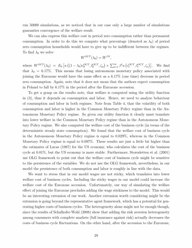
We can also express this welfare cost in period zero consumption rather than permanent

consumption. In order to do this we compute what percentage (denoted as λ0) of period

zero consumption households would have to give up to be indifferent between the regimes.

To find λ0 we solve

WOUT (λ0) = W IN ,

where WOUT (λ0) = E0

[u((1− λ0)cOUT0 , lOUT0 , ζ0

)+∑∞

t=1 βtu(cOUTt , lOUTt , ζt

)]. We find

that λ0 = 6.17%. This means that losing autonomous monetary policy associated with

joining the Eurozone would have the same effect as a 6.17% (one time) decrease in period

zero consumption. Again, note that it does not mean that the authors expect consumption

in Poland to fall by 6.17% in the period after the Eurozone accession.

To get a grasp on the results note, that welfare is computed using the utility function

in (3), thus it depends on consumption and labor. Hence, we need to analyse behaviour

of consumption and labor in both regimes. Note from Table 4, that the volatility of both

consumption and labor is higher in the Common Monetary Policy regime than in the Au-

tonomous Monetary Policy regime. So given our utility function it clearly must translate

into lower welfare in the Common Monetary Policy regime than in the Autonomous Mone-

tary Policy regime. We also computed the welfare cost of the business cycle (in terms of the

deterministic steady state consumption). We found that the welfare cost of business cycle

in the Autonomous Monetary Policy regime is equal to 0.029%, whereas in the Common

Monetary Policy regime is equal to 0.097%. These results are just a little bit higher than

the estimates of Lucas (1987) for the US economy, who calculates the cost of the business

cycle at 0.01%, but the US economy is more stable. Furthermore, Storesletten et al. (2001)

use OLG framework to point out that the welfare cost of business cycle might be sensitive

to the persistence of the variables. We do not use the OLG framework, nevertheless, in our

model the persistence of both consumption and labor is roughly in line with the data.

We want to stress that in our model wages are not sticky, which translates into lower

welfare cost of business cycles. Including the sticky wages in our model could increase the

welfare cost of the Eurozone accession. Unfortunately, our way of simulating the welfare

effect of joining the Eurozone precludes adding the wage stickiness to the model. This would

be an interesting extension of our work. Another extension worth considering might be the

extension is going beyond the representative agent framework, which has a potential for gen-

erating higher costs of business cycles. The heterogeneity alone might not be enough though,

since the results of Schulhofer-Wohl (2008) show that adding the risk aversion heterogeneity

among consumers with complete markets (full insurance against risk) actually decreases the

costs of business cycle fluctuations. On the other hand, after the accession to the Eurozone,

29

the volatilities of shocks hitting the Polish economy may fall and their correlations with

the Eurozone counterparts may increase21. The inclusion of these possible changes into our

simulations should result in lower estimates of costs of losing autonomous monetary policy.

4.3 Decomposition of Volatility Changes

In this subsection we decompose the change in volatility of the main macroeconomic variables

into separate factors related to the Eurozone accession presented on page 26. We stress that

the simulations run here are used only for the purpose of isolating the effects of different

factors that are involved in joining the Eurozone. In order to achieve the desired isolation,

while making those simulations, we make counter-factual assumptions.

First, as the starting point for the decomposition of the variance we use the results

from the simulation Out. These results are presented in Table 6 in the column denoted as

“Simulation 1”.

Second, we compute the effect of the change of the Taylor rule parameters. The Eurozone

Taylor rule differs from the Polish Taylor rule in two important ways: (1) it is more inflation

oriented; and (2) the extend of the of the interest rate smoothing is higher. To isolate this

effect we run the following simulation. We keep everything exactly the same as in the first

simulation, but the parameters of the NBP Taylor rule. We replace the parameters of the

NBP Taylor rule with the parameters from the ECB Taylor rule. This experiment allows us

to say how the standard deviations of the main macroeconomic variables would change if the

NBP ran autonomous monetary policy (responding to the Polish variables only), but with

the same parameters as the ECB. The results of this simulation are presented in Table 6 in

the column denoted as “Simulation 2”. To see the effect of this change compare the results

from the first and second simulations. This change leads to lower variability of inflation and

greater variability of GDP. This is not surprising given that the Taylor rule changes from more

GDP oriented to more inflation oriented. Greater variability of GDP translates into greater

variability of the real side of the economy, i.e. the standard deviations of consumption and

labor increase. Also, greater interest rate smoothing combined with more inflation oriented

monetary policy and smaller variability of inflation reduces the standard deviation of the

interest rate.

Third, we analyse the effect of the replacement of the domestic monetary policy shock

with the foreign monetary policy shock. Thus, we make only modification comparing to

the second simulation. We replace the value of the variance of the monetary policy shock

(estimated for the Polish economy) with the corresponding value from the Eurozone. The

purpose of this exercise is to isolate the effect of smaller volatility of the monetary policy

21In the study we assumed no correlation between shocks in the Eurozone and Poland.

30

Table 5: The decomposition of the volatility changes.Variables Simulation 1 Simulation 2 Simulation 3 Simulation 4

GDP 0.0262 0.0317 0.0286 0.0272Inflation 0.0242 0.0152 0.0129 0.0096Interest rate 0.0211 0.0126 0.0106 0.0294Consumption 0.0133 0.0158 0.0138 0.0225Labor 0.0130 0.0133 0.0132 0.0142

shock in the Eurozone than in Poland. The results of this simulation are presented in Table 6

in the column denoted as “Simulation 3”. This change reduces the volatility of the economy,

which is pretty intuitive, since the standard deviation of the monetary policy shock declines

from 0.01 to 0.002.

Finally, we isolate the effects of fixing of the exchange rate combined with the adoption

of the common monetary policy rule - as shown in equation (44)22. Fixing of the exchange

rate has two effects for the economy: on the one hand it means losing an instrument that

can cushion some external shocks to the economy (for example the shock to foreign demand

for domestic output) but on the other hand the exchange rate risk affects negatively both

exporters and importers. Therefore, depending on the strength of these two effects fixing

the exchange rate may reduce or increase the volatility of the economy. While the effect

of the fixing of the exchange rate is uncertain the effect of the adoption of the common

monetary policy rule is clear. Since the common monetary policy rule reacts to the extended

Eurozone variables rather than the Polish ones, it is less fit to stabilize the Polish economy.

Thus, the adoption of the common monetary policy rule increases the volatility of the Polish

economy23. Summing up, using theory we cannot determine the direction of the changes

created by these effects and we have to rely on numerical simulations. The results of this

simulation are presented in Table 6 in the column denoted as “Simulation 4”. In fact this

is the final change, thus this simulation is exactly the same as the simulation IN in the

previous subsection. These results show that the volatility of GDP decreases and some of

its components become more stable and some less stable. In particular the volatility of

consumption, investment, and imports goes up by, respectively, 63%, 21%, and 113% and

the volatility of exports goes down by 53% (as the volatility of the real exchange rate declines

by 72%). Also, the volatility of inflation decreases. On the other hand, the results show that

the exchange rate absorbs some of the volatility of the interest rate, thus fixing it leads to an

increase of the volatility of the interest rate differential (due to risk premium), which in turn

22Due to technical reasons - violation of the Blanchard-Khan conditions - we were not able to separatethese two effects.

23This claim is also supported by the result of the next section were we show how the change of weight ofthe Polish economy in the common monetary policy rule changes the volatility of Polish variables.

31

translates into higher volatility of the domestic interest rate. Moreover, since the volatility

of consumption and labor is higher, the relative impact of higher volatility the interest rate

on consumption and labor is stronger than the impact of smaller volatility of GDP.

4.4 Sensitivity Analysis

In this subsection we analyse the effect of an increase of the weight of Polish variables in the

extended Eurozone Taylor rule from the GDP share - ωT = 2.97% - to the population share

- ω′T = 10.76%. The results of the new simulation are presented in Table 6. Basically the

results are pretty much the same as previously. Furthermore, the welfare cost of joining the

Eurozone drops only slightly from λ = 0.068% to λ′

= 0.066% of the lifetime consumption,

or differently from λ0 = 6.17% to λ′

0 = 5.99% of the period zero consumption. This only

slightly lessens the macroeconomic consequences of losing autonomous monetary policy after

the Eurozone accession.

Table 6: The weight of Poland and variability of the Polish business cycle.

VariablesAutonomous

Monetary Policy

CommonMonetary Policy

(ωT = 2.97%)

CommonMonetaryPolicy(ω′T = 10.76%)

GDP 0.0276 0.0327 0.0325Inflation 0.0288 0.0098 0.0097Interest Rate 0.0261 0.0300 0.0299Consumption 0.0106 0.0208 0.0206Labor 0.0119 0.0134 0.01335

5 Conclusion

The Eurozone accession for Poland might be costly, since it means losing monetary policy

as a tool to smooth out the business cycles. We build a two country dynamic stochastic

general equilibrium model to quantify the effect of the loss of the autonomous monetary

policy. In our model there are nominal rigidities in the form of sticky prices, which makes

monetary policy not neutral in the short run. There are numerous effects associated with

the Eurozone accession. This study focuses on the effects of losing autonomous monetary

policy on the business cycle behaviour of the main macroeconomic variables and welfare. It

is not a complete study of all the cost and benefits of the Euro adoption.

Since the evidence that higher fluctuations cause lower economic growth is scarce, we

assumed that changes in the business cycle behaviour will not have any long run effect on

the Polish economy. We focused on the change in the business cycle behaviour of the main

32

macroeconomic variables. We found that after Poland joins the Eurozone, the volatility

of GDP increases - the standard deviation of GDP goes up from 2.62% to 2.72%, and the

volatility of inflation decreases - the standard deviation of inflation goes down from 2.41% to

0.96%. We additionally present how different factors involved with the Eurozone accession

affect these outcomes.

We also calculated the impact of this change on the consumers welfare and we found that

the regime change has the same effect as the decline of consumption in the period after the

Eurozone accession by 6.17% (or a decline of lifetime consumption by 0.068%). Moreover, we

checked how the weight of the Polish economy in the decisions of the ECB affects the results

and we found that the increase in weight from 2.93% (which is equal to the GDP share) to

10.76% (which is equal to the population share) lessens the cost of joining the Eurozone, but

the difference is tiny.

Furthermore, our analysis suggest that it is not enough to look at GDP and inflation

to judge the impact of the autonomous monetary policy loss on the economy, because the

changes in business cycle behaviour of consumption, labor and the interest rate might be

greater and more important, from the welfare perspective.

We want to stress that in our model wages are flexible, which, most likely, means that

our result underestimates the cost of joining the Eurozone. Another restriction that might

affect the results is the existence of the representative agent - relaxing this restriction could

increase the cost of business cycle fluctuations and might affect the costs of the Eurozone

accession. Additionally, the introduction of unemployment into the concept of equilibrium

(like e.g. in the search-matching framework) might also positively affect the costs of business

fluctuations. On the other hand, the costs may be lower, if the accession to the Eurozone

increases correlations of shocks or decreases their volatilities. We leave these extensions for

future research.

References

Adolfson, M., Lasen, S., Lind, J., and Villani, M. (2005). ‘Bayesian estimation of an

open economy DSGE model with incomplete pass-through’, Working Paper Series 179,

Sveriges Riksbank (Central Bank of Sweden), http://www.riksbank.com/templates/

Page.aspx?id=16114.

Altig, D., Christiano, L., Eichenbaum, M., and Linde, J. (2005). ‘Firm-specific capital,

nominal rigidities and the business cycle’, NBER Working Papers 11034, National Bureau

of Economic Research, http://www.nber.org/papers/w11034.

Barlevy, G. (2004a). ‘The cost of business cycles and the benefits of stabilization: A survey’,

33

NBER Working Papers 10926, National Bureau of Economic Research, http://www.nber.

org/papers/w10926.

Barlevy, G. (2004b). ‘The cost of business cycles under endogenous growth’, American Eco-

nomic Review, 94 (4), pp. 964–990.

Brooks, S., and Gelman, A. (1998). ‘Some issues in monitoring convergence of iterative

simulations’, in Proceedings of the Section on Statistical Computing, American Statistical

Association.

Ca’ Zorzi, M., De Santis, R. A., and Zampolli, F. (2005). ‘Welfare implications of joining a

common currency’, Working Paper Series 445, European Central Bank, http://www.ecb.

europa.eu/pub/pdf/scpwps/ecbwp445.pdf.

Calvo, G. (1983). ‘Staggered prices and in a utility-maximizing framework’, Journal of Mon-

etary Economics, 12 (3), pp. 383–398.

Carlstrom, C. T., and Fuerst, T. S. (2005). ‘Investment and interest rate policy: a discrete

time analysis’, Journal of Economic Theory, 123 (1), pp. 4–20.

Chari, V. V., Kehoe, P. J., and McGrattan, E. R. (2002). ‘Can sticky price models generate

volatile and persistent real exchange rates?’, Review of Economic Studies, 69 (3), pp. 533–

63.

Chari, V. V., Kehoe, P. J., and McGrattan, E. R. (2007). ‘Business cycle accounting’, Econo-

metrica, 75 (3), pp. 781–836.

Choueiri, N., Murgasova, Z., and Szkely, I. (2005). ‘Republic of Poland: selected issues’, IMF

Country Report 05/264, International Monetary Fund.

Christiano, L. J., Eichenbaum, M., and Evans, C. L. (2005). ‘Nominal rigidities and the

dynamic effects of a shock to monetary policy’, Journal of Political Economy, 113 (1), pp.

1–45.

Christiano, L. J., Eichenbaum, M., and Vigfusson, R. (2003). ‘What happens after a tech-

nology shock?’, NBER Working Papers 9819, National Bureau of Economic Research,

http://www.nber.org/papers/w9819.

Daras, T., and Hagemejer, J. (2008). ‘The long-run effects of the Poland’s accession to the

eurozone’, mimeo, National Bank of Poland.

Erceg, C. J., Henderson, D. W., and Levin, A. T. (2000). ‘Optimal monetary policy with

staggered wage and price contracts’, Journal of Monetary Economics, 46 (2), pp. 281–313.

34

Faruqee, H. (2004). ‘Measuring the trade effects of EMU’, IMF Working Papers 04/154, Inter-

national Monetary Fund, http://www.imf.org/external/pubs/ft/wp/2004/wp04154.

pdf.

Frankel, J., and Rose, A. (2002). ‘An estimate of the effect of common currencies on trade

and income’, The Quarterly Journal of Economics, 117 (2), pp. 437–466.

Goodfriend, M., and King, R. G. (1998). ‘The new neoclassical synthesis and the role of

monetary policy’, Working Paper 98-05, Federal Reserve Bank of Richmond, http://www.

richmondfed.org/publications/research/working_papers/1998/pdf/wp98-5.pdf.

Hastings, W. (1970). ‘Monte Carlo sampling methods using Markov chains and their appli-

cations’, Biometrica, 57 (1), pp. 97–109.

Hodrick, R. J., and Prescott, E. C. (1997). ‘Postwar U.S. business cycles: An empirical

investigation’, Journal of Money, Credit and Banking, 29 (1), pp. 1–16.

Juillard, M. (1996). ‘Dynare : a program for the resolution and simulation of dynamic models

with forward variables through the use of a relaxation algorithm’, CEPREMAP Working

Papers (Couverture Orange) 9602, CEPREMAP, http://www.cepremap.cnrs.fr/couv_

orange/co9602.pdf.

Karam, P., Laxton, D., Rose, D., and Tamirisa, N. (2008). ‘The macroeconomic costs and

benefits of adopting the euro’, IMF Staff Papers, 55 (2), pp. 339–355.

Kolasa, M. (2008). ‘Structural heterogenity of assymetric Shocks? Poland and the Euro Area

through the lens of a two-country DSGE model’, NBP Working Papers 49, National Bank

of Poland, http://www.nbp.pl/publikacje/materialy_i_studia/49_en.pdf.

Kydland, F. E., and Prescott, E. C. (1982). ‘Time to build and aggregate fluctuations’,

Econometrica, 50 (6), pp. 1345–70.

Lopes, A. F. (2007). ‘The costs of EMU for transition countries’, Money Macro and Finance

(MMF) Research Group Conference 2006 2, Money Macro and Finance Research Group,

http://repec.org/mmf2006/up.7815.1140017467.pdf.

Lucas, R. E. (1976). ‘Econometric policy evaluation: A critique.’, Carnegie-Rochester Con-

ference Series on Public Policy, 1, pp. 19–46.

Lucas, R. E. (1987). Models of business cycles. Oxford: Basil Blackwell.

McDaniel, C. A., and Balistreri, E. J. (2003). ‘A discussion on Armington trade substitution

elasticities’, Computational Economics 0303002, EconWPA.

35

Metropolis, N., Rosenbluth, A., Rosenbluth, M., Teller, A., , and Teller, E. (1953). ‘Equations

of state calculations by fast computing machines’, Journal of Chemical Physics, 21 (6), pp.

1087–1092.

Rabanal, P., and Tuesta, R. V. (2007). ‘Non tradable goods and the real exchange rate’,

”la Caixa” Working Paper 03/2007, Caja de Ahorros y Pensiones de Barcelona, http:

//ssrn.com/abstract=1018864.

Rose, A. K. (2000). ‘One money, one market: the effect of common currencies on trade’,

Economic Policy, 15 (30), pp. 7–46.

Ruhl, K. (2005). ‘Solving the elasticity puzzle in international economics’, mimeo, University

of Texas.

Schmitt-Grohe, S., and Uribe, M. (2003). ‘Closing small open economy models’, Journal of

International Economics, 61 (1), pp. 163–185.

Schulhofer-Wohl, S. (2008). ‘Heterogeneous risk preferences and the welfare cost of business

cycles’, Review of Economic Dynamics, 11 (4), pp. 761–780.

Smets, F., and Wouters, R. (2003). ‘An estimated dynamic stochastic general equilibrium

model of the euro area’, Journal of the European Economic Association, 1 (5), pp. 1123–

1175.

Storesletten, K., Telmer, C. I., and Yaron, A. (2001). ‘The welfare cost of business cycles

revisited: Finite lives and cyclical variation in idiosyncratic risk’, European Economic

Review, 45 (7), pp. 1311–1339.

Taylor, J. B. (1980). ‘Aggregate dynamics and staggered contracts’, Journal of Political

Economy, 88 (1), pp. 1–23.

Taylor, J. B. (1993). ‘Discretion versus policy rules in practice’, Carnegie-Rochester Confer-

ence Series on Public Policy, 39, pp. 195–214.

36

Appendix A The log-linearised model

Denote the log deviation of a variable from its deterministic steady state as xt = log(xtx

).

To derive the first order approximation we use the following method

xt = xxtx−1 = xe(log xt−log x) = xelog

xtx = xext ≈ x (1 + xt)

A.1 Households

Capital accumulation. From (6) we obtain

ˆkt+1 = (1− δ) ˆkt + δxt (A.1)

ˆk∗t+1 = (1− δ∗) ˆk∗t + δ∗x∗t (A.2)

Capital supply. From (7) we obtain

kt =ut + ˆkt (A.3)

k∗t =u∗t + ˆk∗t (A.4)

Tobin’s Q. From (11) we obtain

xt =ι

1 + βQt +

β

1 + βEtxt+1 +

1

1 + βxt−1 (A.5)

x∗t =ι∗

1 + β∗Q∗t +

β∗

1 + β∗Etx

∗t+1 +

1

1 + β∗x∗t−1 (A.6)

Euler equation. From (12) we obtain

σEt (ct+1 − ct) =Et

[rt+1 − Qt − β(1− δ)

(rt+1 − Qt+1

)](A.7)

σ∗Et(c∗t+1 − c∗t

)=Et

[r∗t+1 − Q∗t − β∗(1− δ∗)

(r∗t+1 − Q∗t+1

)](A.8)

Capital utilization. From (13) we obtain

rt =Ψ′′ (1)

β−1 − (1− δ)ut (A.9)

r∗t =Ψ′′ (1)∗

(β∗)−1 − (1− δ∗)u∗t (A.10)

37

No arbitrage, capital and nominal assets. From (15) we obtain

σEt (ct+1 − ct) =Et

(Rt − πt+1

)(A.11)

σ∗Et(c∗t+1 − c∗t

)=Et

(R∗t − π∗t+1

)(A.12)

No arbitrage, home and international assets. From (15) we obtain

Rt − R∗t =Et[(qt+1 − qt) +

(πt+1 − π∗t+1

)]+ κt (A.13)

Risk premium. From (4) we obtain

κt = χd¯GDP

(dt − ˆGDP t

)+ εκ,t (A.14)

Labor market. From (9) and (10) we obtain

σct + γlt + ζt =wt (A.15)

σ∗c∗t + γ∗l∗t + ζt∗

=w∗t (A.16)

A.2 Producers

Denote pH,t =PH,tPt

, pF,t =PF,tPt

, pH,t =P ∗H,tP ∗t

, p∗F,t =P ∗F,tP ∗t

, and dt =etD∗H,t+1

Pt

Demand for homogeneous intermediate goods. From (19) and (20) we obtain

YH,t =− 1 + µ

µpH,t + Yt (A.17)

YF,t =− 1 + µ

µpF,t + Yt (A.18)

Y ∗H,t =− 1 + µ∗

µ∗p∗H,t + Y ∗t (A.19)

Y ∗F,t =− 1 + µ∗

µ∗p∗F,t + Y ∗t (A.20)

The inflation of intermediate goods prices. From the definition of relative price pd,t =Pd,tPt

and inflation of sector d intermediate good prices πd,t =Pd,tPd,t−1

, d ∈ {H,F} we obtain.

πH,t =πt + pH,t − pH,t−1 (A.21)

πF,t =πt + pF,t − pF,t−1 (A.22)

38

and

π∗F,t =π∗t + p∗F,t − p∗F,t−1 (A.23)

π∗H,t =π∗t + p∗H,t − p∗H,t−1 (A.24)

Final goods producers. From (21) we obtain

πt = (1− η) (pF )−1µ (πF,t + pF,t−1) + η (pH)

−1µ (πH,t + pH,t−1) (A.25)

π∗t =η∗ (p∗F )−1µ(π∗F,t + p∗F,t−1

)+ (1− η∗) (p∗H)

−1µ(π∗H,t + p∗H,t−1

)(A.26)

Marginal costs of heterogeneous intermediate goods. From (31) we obtain

mct =αrt + (1− α) (wt − zt) (A.27)

mc∗t =α∗r∗t + (1− α∗) (w∗t − z∗t ) (A.28)

Optimal production factors employment. From (32) we obtain

rt − wt =lt − kt (A.29)

r∗t − w∗t =l∗t − k∗t (A.30)

Prices of heterogeneous intermediate goods. From (35) and (36) we get home goods

prices:

pH,t =θH

1 + βθ2H

(pH,t−1 − πt) +βθH

1 + βθ2H

Et (pH,t+1 + πt+1)

+(1− θH) (1− βθH)

1 + βθ2H

mct (A.31)

p∗H,t =θ∗H

1 + β(θ∗H)2

(p∗H,t−1 − π∗t

)+

βθ∗H1 + β(θ∗H)2

Et(p∗H,t+1 + π∗t+1

)+

(1− θ∗H) (1− βθ∗H)

1 + βθ2H

(mct − qt) (A.32)

39

and foreign goods prices

p∗F,t =θ∗F

1 + β∗(θ∗F )2

(p∗F,t−1 − π∗t

)+

β∗θ∗F1 + β∗(θ∗F )2

Et(p∗F,t+1 + π∗t+1

)+

(1− θ∗F ) (1− β∗θ∗F )

1 + β∗(θ∗F )2mc∗t (A.33)

pF,t =θF

1 + β∗(θF )2(pF,t−1 − πt) +

β∗θF1 + β∗(θF )2

Et (pF,t+1 + πt+1)

+(1− θF ) (1− β∗θF )

1 + β∗(θF )2(mc∗t + qt) (A.34)

Aggregate Production function. From (28) and (22) we obtain

YH

Akα(zl)1−α YH,t +

(1− YH

Akα(zl)1−α

)Y ∗H,t =αkt + (1− α)

(zt + lt

)(A.35)

Y ∗F

A∗(k∗)α (

z∗l∗)1−α YF,t +

(1− Y ∗F

A∗(k∗)α (

z∗l∗)1−α

)Y ∗F,t =α∗k∗t + (1− α∗)

(z∗t + l∗t

)(A.36)

A.3 Government

Government expenditures. From (37) we obtain

Gt =ρGGt−1 + εG,t (A.37)

G∗t =ρ∗GG∗t−1 + ε∗G,t (A.38)

A.4 Central Bank

Taylor rule. From (38) we obtain

Rt =γRRt−1 + (1− γR)(γππt + γy ˆGDP t + γdGDP

ˆdGDP t + γdπdπt

)+ ϕt (A.39)

R∗t =γ∗RR∗t−1 + (1− γ∗R)

(γ∗ππ

∗t + γ∗y ˆGDP

∗t + γ∗dGDP

ˆdGDP∗t + γ∗dπdπ

∗t

)+ ϕ∗t (A.40)

40

A.5 Closing the model

Market clearing. From (39) we obtain

C

YCt +

X

YXt +

G

YGt +

rk

Yut =Yt (A.41)(

C

Y

)∗C∗t +

(X

Y

)∗X∗t +

(G

Y

)∗G∗t +

(rk

Y

)∗u∗t =Y ∗t (A.42)

Balance of Payments. From (40) we obtain

1− ωω

(qp∗H

1−ωωY ∗H

¯GDP

)(qt + p∗H,t + Y ∗H,t

)+

(d¯GDP

)β∗

π∗

(dt − R∗t − κt

)=

=

(pF YF

¯GDP

)(pF,t + YF,t

)+

(d¯GDP

)1

π∗

(dt−1 + qt − qt−1 − π∗t

)(A.43)

GDP. From (41) we obtain

ˆGDP t =

(Y¯GDP

)Yt +

1− ωω

(qp∗H

1−ωωY ∗H

¯GDP

)(p∗H + Y ∗H + qt)−

(pF YF

¯GDP

)(pF + YF ) (A.44)

ˆGDP∗t =

(Y ∗

¯GDP∗

)Y ∗t +

(pF

ω1−ω YF

q ¯GDP∗

)(pF + YF − qt)−

p∗H Y∗H

¯GDP∗ (p∗H + Y ∗H) (A.45)

Appendix B Welfare Cost Computation

Here we describe the details of computing λ. First notice that it is much more convenient

to solveWOUT (λ)

c1−σ =W IN

c1−σ , (B.1)

rather than (48). Next we split total utility into utility from consumption and disutility from

work. Then for any regime Θ ∈ {IN,OUT}

WΘ(λ)

c1−σ = E0

[∞∑t=0

βt((1− λ)cΘ

t

)1−σ

1− σ

]− E0

[∞∑t=0

βtψζt

(lΘt)1+γ

1 + γ

]

=WC,Θ(λ)

c1−σ − WL,Θ

c1−σ

where WC,Θ(λ)c1−σ

= E0

[∑∞t=0 β

t ((1−λ)cΘt )1−σ

1−σ

]and WL,Θ

c1−σ= E0

[∑∞t=0 β

tψζt(lΘt )

1+γ

1+γ

]. It is conve-

nient to denote WC,Θ(1) ≡ WC,Θ, than WC,Θ(λ)c1−σ

= (1 − λ)1−σ WC,Θ

c1−σ. To find WC,Θ

c1−σand WL,Θ

c1−σ

41

first notice that (9) and (10) imply that in the deterministic steady state

%c1−σ = ψl1+γ (B.2)

After the straightforward computations of the equilibrium conditions in the deterministic

steady state we get that

% =(1− α) [1− β(1− δ)]

αδβ

(xy

)(cy

)which we calibrated to match the deterministic steady state relationships and we found that

% = 1.09. Next we used (B.2) to find the following

WC

c1−σ =∑

βt(ctc

)1−σ

1− σ=∑

βt(exp(ct))

1−σ

1− σ

WL

c1−σ =∑

βtψζt

l1+γt

c1−σ

1 + γ=∑

βtψζt

l1+γt

ψ%l1+γ

1 + γ=∑

βt%ζt

(ltl

)1+γ

1 + γ=∑

βt%ζt

(exp(lt)

)1+γ

1 + γ

Notice that with this formula it is not necessary to find the deterministic steady state values

of c or l.

To find the welfare cost expressed in period zero consumption λ0 we use analogous

method. The only difference is that (B.1) is replaced with

WOUT (λ0)

c1−σ =W IN

c1−σ ,

where

WΘ(λ0)

c1−σ = E0

[((1− λ0)cΘ

0

)1−σ

1− σ

]+ E0

[∞∑t=1

βt(cΘt

)1−σ

1− σ

]− E0

[∞∑t=0

βtψζt

(lΘt)1+γ

1 + γ

]

= (1− λ0)(1− β)WC,Θ

c1−σ + βWC,Θ

c1−σ −WL,Θ

c1−σ .

42