The Macroeconomics of Downward Nominal Wage … · period 1956-2011. This evidence suggests that the real world is more Tobin-like than classical, implying that the permanent unemployment

Fortin : Département des sciences économiques, Université du Québec à Montréal; CIRPÉE

[email protected]

Revision of a paper prepared for Thinking Outside the Box, a Conference in Celebration of Tom Courchene held at

Queen’s University, Kingston, Ontario, on October 26 and 27, 2012. Without implicating them, I thank George

Akerlof, Allan Crawford, Ramdane Djoudad, Karine Dumont, Lynda Khalaf, Jimmy Royer, Marcel Voia,

Christopher Ragan, Beth Anne Wilson, and especially Tim Sargent, for advice and comments.

Cahier de recherche/Working Paper 13-09

The Macroeconomics of Downward Nominal Wage Rigidity : a Review

of the Issues and New Evidence for Canada

Pierre Fortin

Avril/April 2013

Abstract: Inflation definitely has costs, but they remain difficult to quantify for rates below 10-15 per cent. Aiming for a low rate of inflation, as Canada has done in the last 20 years, carries with it various risks, such as debt deflation, reduced flexibility of interest rates, and downwardly rigid nominal wages. In this paper, I focus on the latter problem. As James Tobin pointed out in 1972, economy-wide downward nominal wage rigidity generates a long-run negative relation between inflation and unemployment, implying that permanently low inflation can be bought only at the cost of permanently high unemployment. In contrast, the classical assumption of full wage flexibility implies that low inflation carries no permanent unemployment costs. The literature has produced compelling evidence that firm and worker resistance to nominal wage cuts is fierce, extensive and persistent in advanced economies, including Canada. But the macroeconomic significance of this phenomenon is still disputed. After presenting the details of the competing classical and Tobin views on wage flexibility or rigidity, I review the theoretical and empirical objections to the macroeconomic relevance of downward nominal wage rigidity that can be found in the literature. I then present new macroeconomic evidence on the matter based on Canadian macrodata for the 56-year period 1956-2011. This evidence suggests that the real world is more Tobin-like than classical, implying that the permanent unemployment costs of aiming for a low rate of inflation such as the current 2-per-cent target could be significant. According to the results I obtain, sticking to this target would keep the national unemployment rate between 1.0 and 2.7 percentage points in excess of the asymptotic minimum rate that would be attainable at a somewhat higher inflation rate. Keywords: Wage rigidities, Canadian Phillips Curve, Inflation-unemployment trade off JEL Classification: E24, E31, E58 Résumé: Les coûts de l’inflation sont réels, mais ils demeurent difficiles à quantifier pour des taux inférieurs à 10 ou 15 %. Adopter une cible d’inflation faible, comme le Canada l’a fait depuis vingt ans, entraîne certains risques, comme la déflation des dettes, une flexibilité réduite des taux d’intérêt et la rigidité à la baisse des salaires nominaux. C’est ce dernier problème qui fait l’objet de la présente étude. En 1972, James Tobin a fait remarquer qu’une rigidité à la baisse généralisée des salaires nominaux dans l’économie engendre une relation à long terme négative entre l’inflation et le chômage. En l’occurrence, cela voudrait dire qu’un taux d’inflation permanent faible ne pourrait s’obtenir qu’au coût d’un taux de chômage permanent élevé. À l’opposé, l’hypothèse classique de flexibilité des salaires signifie qu’un taux d’inflation faible n’entraîne aucun coût permanent en chômage élevé. La littérature a produit plusieurs preuves que la résistance des entreprises et des travailleurs à des coupes de salaires nominaux est forte, répandue et persistante dans les économies avancées, Canada compris. Toutefois, les conséquences macroéconomiques de ce phénomène sont encore débattues. Après avoir présenté le détail de la vision classique et de l’hypothèse de Tobin, respectivement sur la flexibilité et la rigidité des salaires, je passe en revue les objections théoriques et empiriques à la pertinence macroéconomique de la rigidité à la baisse des salaires nominaux qui ressortent de la littérature. Je présente ensuite sur la question de nouveaux résultats statistiques basés sur les données macroéconomiques canadiennes de la période de 56 années de 1956 à 2011. Ces résultats permettent de

croire que le monde réel ressemble plus à celui de Tobin qu’à la vision classique. Le coût permanent, en chômage accru, de réaliser un taux d’inflation comme celui de 2 % qui est présentement visé au Canada pourrait s’avérer important. Selon les résultats obtenus, adhérer à une telle cible d’inflation maintiendrait le taux de chômage canadien à un niveau qui serait supérieur de 1,0 à 2,7 unités de pourcentage au taux minimum pouvant être atteint asymptotiquement à un niveau d’inflation un peu plus élevé.

The French engineer and mathematician Maurice Allais, who laid out the foundations of

modern general equilibrium and welfare theory in the 1940s, chided contemporary

economics for what he called its love story with mathematical charlatanry, its

econometric savagery, its ignorance of economic history, and its lack of a broader social

science culture (Allais 1989). Tom Courchene has avoided all these pitfalls. For forty

years now, he has contributed to an incredible number of areas, from monetary and fiscal

policy to taxation, social policy, trade policy, financial regulation, competition policy,

constitutional matters, human capital, pensions, environmental issues, regional growth,

First Nations’ future, etc. His thinking has been influential in all of these areas and in

every part of the country and beyond. He is not just another economist. He is a national

treasure. And he is an important reason that Queen’s has remained a dominant Canadian

institution in the study of public policy over the past quarter century.

Between 1975 and 1983, Tom wrote five monographs on the conduct of Canadian

monetary policy under then-governor Gerald Bouey. This Conference provides me with

the opportunity to return to a key concern in this area, namely the macroeconomic trade-

off between inflation and unemployment that is crucial for the design and conduct of

monetary policy, and that we commonly call the Phillips curve (after Phillips 1958).

I proceed as follows. In section 1, I state the main message of the economic literature on

the costs of inflation, which is that these costs definitely do exist, but that they remain

difficult to quantify for rates below 10-15 per cent. Section 2 adds the concern that

aiming for a very low rate of inflation, as Canada has done in the last 20 years, carries

with it various risks, such as debt deflation, reduced flexibility of interest rates, and

downwardly rigid nominal wages. Section 3 explains how, in contrast to the classical

assumption of full wage flexibility, money illusion leading to downward nominal wage

rigidity generates a long-run negative relation between inflation and unemployment. This

implication, underlined by James Tobin in 1972, would mean that permanently low

inflation can be bought only at the cost of permanently high unemployment. Section 4

reviews the evidence that this resistance is extensive and persistent in advanced

economies, including Canada, but points out that the literature is still uncertain about the

macroeconomic significance of downward nominal wage rigidity. The later sections of

the paper are concerned with this question of macroeconomic relevance, particularly in

the Canadian context. Sections 5 and 6 present the theoretical details of the different

implications of the competing classical and Tobin views of the long-run Phillips curve.

Sections 7 and 8 review the theoretical and empirical objections to the macroeconomic

relevance of downward nominal wage rigidity found in the literature. Finally, section 9

presents new macroeconomic evidence on the matter based on Canadian macrodata for

the 56-year period 1956-2011. This evidence suggests that the real world is more Tobin-

like than classical. It implies that the permanent unemployment costs of aiming for a low

rate of inflation such as 2 percent could be significant.

1 High inflation definitely has costs, but their exact magnitude remains uncertain

Canada first set an official inflation target in February 1991. The Minister of Finance and

the Governor of the Bank of Canada jointly announced that the Bank would aim to

reduce CPI inflation to 2 per cent per annum by the end of 1995 (Bank of Canada 1991).

In fact, inflation declined to 2 per cent by the end of 1992, much in advance of schedule.

The agreement between the Minister and the Governor was renewed in 1995, 2001, 2006

and 2011. Each time, the official target was kept at 2 per cent, with a control range of 1 to

3 per cent around it. The Bank of Canada has successfully fulfilled its commitment.

Between 1995 and 2012, Canadian CPI inflation has averaged exactly 2.0 per cent, with a

mean deviation of 0.7 point from target.

The point of aiming for a low and stable rate of inflation is that high and variable

inflation has costs. People dislike inflation. They believe inflation erodes their purchasing

power and redistributes income and wealth arbitrarily and unfairly (e.g., Shiller 1997).

Partly, this reflects money illusion, since we know that increases in price inflation are

usually covered by increases in nominal wage growth of similar orders of magnitude.

Nevertheless, the public is not so stupid. As Modigliani (1986) pointed out, “from the

justified proposition that the level of money and prices is neutral in the long run, one

cannot go straight to the conclusion that changes in money and the level of prices cannot

produce real effects for extended periods of time [as this] would ignore some essential

facts of life, such as the existence of nominal contracts, of nominal institutions, and of

nominal habits of thinking and carrying out economic calculations.” Furthermore,

inflation imposes a distortionary tax on holding cash (Bailey 1956). It generates

uncertainty and confusion about present and future relative prices (Fischer and

Modigliani 1978). It can be harmful to saving and investment due to its interaction with a

less-than-fully-indexed tax system (Feldstein 1997).1

However, it has proven difficult to quantify the impact of inflation on economic

performance empirically (e.g., Bernanke, Laubach, Mishkin and Posen 1999). Among

macroeconometric studies, the contribution by Robert Barro (1997) has been the most

influential. His panel study of about 100 countries over 1965-1990 found that inflation

rates above 15 percent were indeed harmful for real growth. But for countries and periods

with average inflation rates below 10-15 per cent, he was not able to detect any

significant effect of inflation on economic performance. Other country panel studies

providing detailed checks on the robustness of this finding have reached similar

conclusions (e.g., Levine and Renelt 1992; Sala-i-Martin 1997).

The picture of inflation that emerges from the existing literature is that people hate it, and

that it may hurt resource allocation and perhaps even growth, but to an extent that

remains difficult to quantify. Whatever the case may be, beginning in 1990 a number of

countries went ahead and committed to achieve specific inflation targets, usually between

2 and 3 per cent. Among advanced industrial countries, New Zealand was the first,

followed by Canada, the United Kingdom, Sweden, Finland, Australia and others. Many

Central European and Latin American countries followed suit. The United States joined

the group of official inflation targeters only recently, in 2012, but it has been argued that

it had in fact been engaged in “covert inflation targeting” since the early 1990s (Mankiw

2001).

1 See Ragan (1998) for a useful survey of these problems in the Canadian context.

The idea of reducing the inflation target below 2 per cent has even received some support

from experiments by Bank of Canada researchers who have constructed artificial,

simulation-based models that have identified benefits from a lower, or even negative,

target rate for inflation. However, the Bank’s management has recognized that their

results “remain subject to considerable uncertainty,” and that their models “typically

abstract from the costs and risks associated with very low rates of inflation.” (Bank of

Canada 2011)

2 Aiming for a very low rate of inflation has risks

What are the risks of maintaining the rate of inflation at 2 per cent or less? First, there is

an upward bias in the measurement of the CPI. In the United States, CPI inflation would

seem to overstate the true rate of inflation by about 1 percentage point per year (Boskin,

Dulberger, Gordon, Griliches and Jorgenson 1996; Lebow and Ruud 2003). In Canada,

the estimated upward bias is 0.5 point per year (Crawford 1998; Sabourin 2012). There is

no real problem here. As long as the rough magnitude of this measurement bias is known,

the U.S. Federal Reserve and the Bank of Canada can readily take it into account in

setting the target rate of inflation.

A more serious risk arises from the fact that setting the inflation target close to zero

increases the probability that the economy be tipped into a Fisher-type “debt-deflation

trap”. Fisher (1933) famously argued that, by increasing the real value of nominal debts,

deflation can create liquidity and solvency problems for borrowers and trigger a credit

contraction and a recession, which can degenerate into a prolonged vicious circle. Periods

of debt deflation have occurred during the Great Depression and, more recently, in Japan

(Bernanke and James 1991; Eggertsson and Krugman 2012).

A third risk stems from the zero lower bound to which interest rates are subject (e.g.,

Summers 1991). Since, on average, a low rate of inflation will induce low interest rates,

the fact that nominal interest rates cannot be negative implies that a lower and lower rate

of inflation leaves less and less room for monetary policy to reduce interest rates in the

face of adverse shocks. Hence, very low inflation increases the probability that the

economy will remain stuck in a recession or even in a liquidity trap for an extended

period.

Until recently, many central bankers did not take the zero-lower-bound risk very

seriously. In 2001, for example, the Bank of Canada reported that “most researchers

would estimate the probability of hitting the zero floor as negligible for an inflation target

of 2 per cent.” (Bank of Canada 2001). However, the experiences of many advanced

countries since 2008 has led the Bank to revise its judgment and recognize that the zero

lower bound on interest rates has become “a binding constraint for many central banks,

which were then forced to use unconventional monetary policy tools, such as

extraordinary forward guidance, quantitative easing and credit easing”, adding that the

cost, reliability and effectiveness of these new, still unconventional, policy tools remain

uncertain. (Bank of Canada 2011)

Summers (1991) concluded his analysis by suggesting that that the optimal inflation rate

might be “as high as 2 or 3 percent.” Later, in discussing the Japanese slump, Krugman

(1998) and Bernanke (2000) suggested that the Bank of Japan pursue “a target in the 3-4

per cent range for inflation, to be maintained for a number of years.” More recently, IMF

economists concurred that the zero lower bound constraint raises the question of whether

the inflation target should be raised, perhaps to 4 per cent (Blanchard, Dell’Ariccia and

Mauro 2010). Some economists continue to think that the 2 per cent target is too high, but

the 2008 crisis has led others to express the opposite worry that it could be too low.

There is a fourth risk from setting the inflation target at too low a level. Various

manifestations of money illusion could generate a long-run trade-off between inflation

and unemployment at low rates of inflation. For economic welfare, this would have the

implication that keeping inflation at a target rate such as 2 per cent or less would require

that the unemployment rate be maintained at a permanently higher level than it would

have to be if the inflation rate target were, say, 3-4 per cent. Permanent unemployment

has permanent costs.

Most central bankers believe that there is no such trade-off. They think that the rate of

inflation monetary policy chooses to aim for has no lasting influence on the rate of

permanent unemployment at which the economy eventually settles. According to this

view, which I will henceforth call the “classical” view, a unique equilibrium rate of

unemployment would exist, and it would not depend on nominal wages and prices or

their rates of change, but only on real factors such as relative prices, productivity,

monopoly and union power, demographics, taxation, social programs, etc.

3 Whether there is a long-run trade-off between inflation and unemployment

matters enormously for economic welfare

The classical, no-long-run-trade-off, view was popularized by Milton Friedman (1968)

and Robert Lucas (1973). Its policy implication is that a central bank can reduce inflation

as low as it wishes by tightening monetary conditions so that unemployment first rises

above its equilibrium value and inflation declines as desired. Then, once the job of

disinflation is done, monetary conditions are eased back. This allows unemployment to

return to the same equilibrium level as prevailed before the experiment began, and

inflation to remain steady at its lower value without further excess unemployment costs.

The national income loss and hurtful unemployment arising from the initial disinflation

may be far from negligible, but once these short-run costs are “behind us”, there are no

further costs to worry. The operation is like a canal treatment, not a permanent backache.

The Friedman-Lucas view of the world is based on the premise that nominal wages and

prices by themselves do not play any meaningful, lasting role in economic decisions, but

matter only when compared to other nominal wages and prices. Many have recognized

that this premise is too extreme and that money illusion is widespread in the real world

(e.g., Fisher 1928; Modigliani 1986; Shafir, Diamond and Tversky 1997). In particular,

forty years ago Eckstein and Brinner (1972) and Tobin (1972) considered instances of

money illusion that they thought could have significant macroeconomic consequences.

Eckstein and Brinner conjectured that 2 per cent is such a low rate of inflation that many

workers and firms would ignore it when setting wages. As inflation would rise, there

would be “increased awareness and concern” with real as opposed to nominal wages, so

that observed inflation would become incorporated more fully into nominal wage

contracts. This phenomenon would give rise to a negatively-sloped permanent relation

between inflation and unemployment at low inflation rates. Then, above some inflation

threshold where wage setters would think fully in real terms, the slope of the relation

would become vertical, which means that the trade-off would disappear and that the

classical world would be back.

The other paper, by James Tobin (1972), considered the possibility that money illusion

would prevent nominal wages from ever declining. Tobin argued that the long-run

Phillips curve would then be “very flat for high unemployment and [become] vertical at a

critically low rate of unemployment.” The reason downwardly rigid nominal wages would

generate a long-run negative relation between inflation and unemployment is that labour

markets are heterogeneous. As inflation declined to low values, the entire distribution of

firm-level nominal wage changes would move down with inflation. A rising fraction of

wage changes would hit the zero wall and would end up being wage freezes instead of

wage cuts. The distribution would be “censored” at zero. As a result, the downward

pressure exerted on aggregate wage growth and inflation by any given increase in the rate

of unemployment would become weaker and weaker. This would force the central bank

to maneuver monetary policy so as to bring unemployment to the higher and higher levels

needed to achieve and maintain every additional point of inflation reduction.

Under money illusion à la Eckstein-Brinner or à la Tobin, targeting a low rate of inflation

such as 2 per cent would carry two kinds of unemployment costs. In addition to the short-

run cost of initially disinflating to 2 per cent, which would also be present in a classical

world, there would be the additional long-run cost of maintaining inflation permanently

at 2 per cent. To get a flavor of the magnitudes involved in the case of Canada, consider

the change of trend inflation from 5 per cent toward the end of the 1980s to 2 per cent by

the mid-1990s. Based on estimates by Mazumder (2012), the output sacrifice that

accompanied the increased unemployment during this disinflation period was 2.75 times

the 3-point decline in trend inflation, or 8.25 per cent of one year’s GDP. According to

this calculation, the cost of reducing inflation to the Canadian economy was about $61

billion.2

This was a large cost, which by 1995 was “behind us”. However, with money illusion the

long-run cost of the policy could be much larger, and it would still be with us today. To

fix ideas, suppose that maintaining inflation permanently at the lower 2 per cent level

instead of, say, 4 per cent had been keeping Canada’s unemployment rate permanently

higher by one percentage point. Then, the capitalized cost of the associated permanent

income loss over time would have been between $555 billion and $740 billion, not

counting the human costs of the permanent addition of over one hundred thousand

2 This estimate is based on an assumption of $740 billion for potential GDP in 1992. Mazumder’s estimate

of the sacrifice ratio is based on Ball’s (1994) methodology.

workers to the ranks of the unemployed.3 These are not small numbers to compare to the

real, but uncertain, benefits from the reduction of inflation from 4 per cent to 2 per cent.

4 Downward nominal wage rigidity: why, how extensive and persistent, and how

relevant macroeconomically?

In the rest of this paper, I study the type of money illusion envisaged by James Tobin,

that is, downward nominal wage rigidity. I will be mainly concerned with its presence

and relevance in the Canadian economy. There are three questions to be addressed: 1)

why workers and firms strongly resist money wage cuts, 2) how important and persistent

this resistance actually is in advanced economies, and 3) how macroeconomically

significant this phenomenon is, particularly in Canada. Answers to the first two questions

will come easily, but there is more uncertainty concerning the problem of

macroeconomic relevance. I will therefore spend more time on this third question and

look for additional evidence in the Canadian context.

The first question to be dealt with is why money wage rollbacks should be relatively rare.

Building on previous research (e.g., Kahneman, Knetsch, and Thaler 1986) and adding

his own survey evidence, Truman Bewley (1999) has provided a clear answer to this

question. Puzzling over the fact that nominal wages had rarely been cut during the 1991

recession in the United States, Bewley interviewed hundreds of managers, labour leaders,

professional recruiters and advisors to the unemployed in 1992 and 1993, and asked them

why. The reason most often reported to him was that workers regard pay cuts as totally

unfair. As a result, firms would be reluctant to cut wages and to replace existing workers

by others, willing to work for less, for fear of losing their good employees and suffering a

serious drop in morale and productivity among their remaining employees. They would

rather cut jobs than wages.

The second question is how extensive and persistent downward nominal wage rigidity

actually is in advanced economies. Again, a clear answer is on hand. It comes from the

International Wage Flexibility Project, which involved 29 researchers from 14 countries

in the early 2000s (Dickens, Goette, Groshen, Holden, Messina, Schweitzer, Turunen and

Ward 2007). The participants scrutinized 360 annual wage change distributions from 31

different datasets covering 16 OECD countries over the period 1972-2003.

The Project’s estimate of labour market heterogeneity relied on the average standard

deviation of measured nominal wage changes across all datasets. After correcting for

measurement errors, it was found to be 7.7 percentage points. The summary statistic used

to infer the extent of downward nominal wage rigidity was the percentage of workers

with pure nominal wage freezes among all those with non-positive wage changes. This

percentage averaged 28 per cent across years and datasets within countries. In the U.S.

Panel Study of Income Dynamics, which was one of the datasets, the percentage of

3 The $740 billion figure comes from applying a 2 per cent Okun coefficient to an estimate of $740 billion

for potential GDP in 1992 and capitalizing the result at a real growth-adjusted discount rate of 2 per cent.

The $555 billion figure is based on an alternative, more conservative, estimate of 1.5 per cent for the Okun

coefficient.

nominal wage freezes was 45 per cent. The authors’ interpretation was that “28 per cent

of the wage cuts that would have taken place under flexible wage setting are prevented by

downward rigidity.” Other authors, such as Fehr and Goette (2005) for Switzerland, Holden

and Wulfsberg (2007) for 19 OECD countries, and Daly, Hobijn and Lucking (2012) for

the United States, have shown that wage cuts are scarce relative to wage freezes even when

inflation has been low for a long period of time. The existence and persistence of downward

nominal wage rigidity now seems to be an established stylized fact of labour markets in

advanced countries.

Unfortunately, Canada was not among the OECD countries covered by the International

Wage Flexibility Project. The reason is that, when the Project got underway, the only

representative Canadian dataset that was suitable for calculating annual wage changes

over an extended period, namely the Survey of Labour and Income Dynamics, was just

beginning to be developed. Given this constraint, many Canadian researchers turned to

the Department of Human Resources and Skills Development’s (HRSDC) database on

wage settlements in bargaining units with 500 or more workers (e.g., Fortin 1996;

Simpson, Cameron and Hum 1998; Crawford and Harrison 1998). Downward nominal

wage rigidity in this dataset is strong and persistent. Over the 31-year period 1982-2012,

86 per cent of first-year non-positive wage changes in large private-sector settlements

have been freezes. Furthermore, this percentage has shown no sign of declining over the

last three decades.4

The obvious problem with data from large unionized firms is that they have special

characteristics and may not be representative of the Canadian labour market.

Employment in these firms accounts for only 7 per cent of total private employment in

Canada. Two datasets with a wider coverage are the short longitudinal files from the

Labour Market Activity Study (LMAS) for 1986-1987 and 1988-1990, which contain

representative samples of the entire household population. One can infer from Bowlus’

(1998) examination of the data in the 1986-1987 file that 29 per cent of non-positive

wage changes reported by job stayers were freezes. This percentage matches the average

percentage of 28 per cent found by the International Wage Flexibility Project. It also

almost surely is an underestimate of the degree of downward nominal wage rigidity in the

Canadian labour market, because it is well-known that household panel data such as the

LMAS seriously overstate the frequency of wage cuts (Akerlof, Dickens and Perry 1996;

4 An OLS regression based on HRSDC’s annual wage settlements data for large private-sector unions for

1982 to 2012 gives the following result:

Rt = 86.8 – 3.3*D9202t – 3.2*D0312t,

(3.1) (4.3) (4.4)

where Rt is the percentage of first-year non-positive wage changes that are freezes in year t; D9202t and

D0312t are dummy variables for 1992-2002 and 2003-2012, respectively; and numbers in parentheses are

standard errors. The p-value for the test that the coefficients of the two dummy variables are both zero is

0.69, which means that the hypothesis that the extent of downward nominal wage rigidity was the same in

the three subperiods 1982-1991 (pre-inflation targeting), 1992-2002 and 2003-2012 cannot be rejected.

Interestingly, the OLS regression result for large public-sector unions over the same time span is :

Rt = 85.0 – 2.7*D9202t – 3.1*D0312t.

(3.5) (4.7) (4.8)

Comparing the two regression results leaves little doubt that the degree and persistence of downward

nominal wage rigidity has been just about the same in the public sector as in the private sector.

Altonji and Devereux 2000; Fehr and Goette 2005). The weight of currently-existing

evidence is that downward nominal wage rigidity is at least as extensive and persistent in

Canada as in the 16 other advanced countries surveyed by the International Wage

Flexibility Project.

While the existence and persistence of downward nominal wage rigidity is no longer in

doubt, the literature is still uncertain about its macroeconomic relevance. It is often asserted,

on the contrary, that it is not relevant. For example, the Bank of Canada has recently stated

that, “while there is some evidence of downward nominal wage rigidities in Canada, their

effects do not appear to be economically significant.” (Bank of Canada 2011). This third

question about downward nominal wage rigidity therefore needs to be carefully examined.

In sections 5 and 6, I will present the different macroeconomic implications of the

competing classical and Tobin views concerning the long-run trade-off between inflation

and unemployment. Then, in sections 7 and 8, I will review the theoretical and empirical

objections to the macroeconomic relevance of downward nominal wage rigidity. Finally,

in section 9, I will report new macroeconomic evidence on the matter based on Canadian

macrodata.

5 According to classical theory, the inflation-unemployment trade-off vanishes in

the long run

To understand how downward nominal wage rigidity can affect the macroeconomic

trade-off between inflation and unemployment, one needs first to recall how inflation and

unemployment would be connected if nominal wages were fully flexible. A fundamental

axiom of classical economic thinking is that nominal wages and prices matter only when

compared to other nominal wages and prices. Only relative wages and prices matter for

nominal wage and price decisions, if not in the short run, where temporary wage and

price misperceptions are possible, then certainly in the long run where the only steady

rate of inflation is the accurately expected one. This classical axiom means that forward-

looking wage setters are concerned not with nominal wages, but with expected real

wages, say w – pe, where w is the nominal wage firms and workers bargain over and p

e is

the price level they expect for the goods they sell and consume, respectively.

In this context, most theories of wage determination (see Bean 1994 for a review)

conclude that, on average at the macro level, the aggregate nominal wage W should be

proportional to the expected price level Pe and expected productivity G

e, a decreasing

function of the unemployment rate U (an indicator of outside opportunities), and also

influenced by a set of other factors X including demographics, taxation, union power, and

labour market institutions and policies.

(1) W = Pe + G

e – aU + X,

where W, Pe and G

e are in logs, and a is a positive parameter.

Given its variable labour cost, the typical firm is assumed to set its price as a

markup (Z) over its marginal cost of production, which, as long as costs are minimized,

can be expressed as the ratio between the wage and the marginal productivity of labour.

This generates a negative connection between the product price and unemployment

because higher unemployment hurts capacity utilization and market power, and increases

labour productivity along the production function. Factors such as taxation, the relative

prices of capital and tradable goods, monopoly power, and various regulations also

impact on productivity G and the markup Z.

(2) P = W – bU – G + Z,

where b is a positive parameter.

Eliminating W from equations (1) and (2) gives a price Phillips curve:

(3) P = Pe – (a + b)(U – U*) + , or =

e – (a + b)(U – U*) + ,

where = P – P-1 and e = P

e – P-1 are actual and expected inflation, U* = (X* + Z*)/(a +

b) is a benchmark unemployment rate, X* and Z* are the steady-state values of X and Z,

and is the zero-mean short-run random disturbance (X – X*) + (Z – Z*) + (Ge – G).

Equation (3) is the formal expression for the short-run trade-off between inflation and

unemployment. Given expected inflation e and benchmark unemployment U*, an

increase of one point in unemployment will cut actual inflation by a + b points per unit of

time. However, this trade-off cannot last forever because price expectations will catch up

with actual inflation. In the steady state, Pe – P =

e – = = 0. Expectations are realized

and the trade-off vanishes. As can be seen from equation (3), the unemployment rate U

settles at the benchmark value U*, which therefore turns out to be its long-run

equilibrium value.

(4) U = U*.

Carrying equation (2) lagged one period into equation (1) leads to another form of trade-

off, this time between aggregate wage growth and unemployment – a wage Phillips

curve:

(5) W = e + G – (a + b)(U – U*) + bU – Z + ,

where W is aggregate nominal wage growth.5

In the steady state, e = , U = Z = = 0 and, from equation (2), W = + G. Hence,

equation (5) has the same implication that U = U* for the long run. Graphically, the long-

run Phillips curve described by equation (4) is a vertical line in unemployment-inflation

5 Working along the New Keynesian tradition, Gali (2011) has proposed a wage Phillips curve with the

same determinants as equation (5). It is based on the staggered wage setting model of Erceg, Henderson

and Levin (2000), in which wages are set unilaterally by a monopoly union. If wages that are not

reoptimized in any given period are automatically indexed to price inflation, and if the unemployment rate

follows a second-order autoregressive process, then an equation similar to (5) is obtained.

plane. In this classical environment, there is no way that a permanently higher rate of

inflation can buy a permanently lower rate of unemployment. We are always eventually

back to the same equilibrium unemployment rate U = U*.

6 Tobin’s theory reinstates the inflation-unemployment trade-off in the long run

What did Tobin (1972) do? He added to the classical model the constraint that nominal

wages can never be rolled back. He envisaged a situation whereby the individual firm

either leaves its wage unchanged from last period’s level, or sets it where the unconstrained

classical response of equation (1) says it should be, whichever is algebraically larger. In

other words, he explored the consequences of assuming that:

(6) w = max(0, wn),

where wn = w

n – w-1 is the unconstrained classical (or notional) log wage change from last

period that the firm would set in the absence of money illusion, and w = w – w-1 is the

actual log wage change, which is constrained never to be negative. Assume for simplicity

that the notional wage changes wn of individual firms are normally distributed

6 with mean

Wn = E(w

n) and variance

2. Then, the resulting actual aggregate wage change W is

readily shown to be:

(7) W = E[max(0, wn)] = W

n(W

n/) + (W

n/) = (W

n/),

where and are the standard normal cumulative distribution and probability density

functions, respectively; is a function defined as (x) x(x) + (x) for all real values

x; and Wn follows the same process as the classical equation (5):

(8) Wn =

e + G – (a + b)(U – U*) + bU – Z + .

As a function of notional aggregate wage change Wn, actual aggregate wage growth W

has three key properties. First, by construction, W always exceeds Wn and never falls

into negative range. Second, W is an increasing and convex function of Wn. Third, as

Wn declines from high to low values, W follows downward, but less than in proportion,

so that the wedge S = W – Wn between them rises. For large enough values of W

n

(depending on the size of ), few individual notional wage changes will be negative. The

wedge S will then be small, actual and notional aggregate wage growth will almost

coincide, and the world will be nearly classical. Conversely, as Wn declines to low values,

a rising fraction of wage changes that would otherwise be negative will be “swept up” to

zero as the Tobin constraint will bite increasingly. The wedge S between W and Wn will

increase. For example, if is equal to 7.7 percentage points, reflecting the overall average of

6 Dickens et al. (2007) found that the Weibull distribution fitted the upper tail of the wage change

distributions in their sample somewhat better than did the normal distribution. However, a Weibull random

variable can take only positive values. Using the Weibull distribution to represent the entire notional wage

change distribution would oddly have to exclude negative wage changes from consideration.

the International Wage Flexibility Project, then Wn = 10 per cent implies W = 10.4 per

cent (S = 0.4 point), while Wn = 3 per cent implies W = 4.8 per cent (S = 1.8 points).

Carrying equation (8) into equation (7) yields the short-run aggregate wage change equation

(or wage Phillips curve) under the assumption that wage decreases are ruled out :

(9) W/ = [(e + G – (a + b)(U – U*) + bU – Z + )/].

The relation between W and U is negatively sloped and convex, and the slope -(a +

b)( Wn/) is smaller than a + b in absolute value.

7 This reflects the fact that

unemployment pressure a + b is effective only over the fraction (Wn/) of notional

wage changes that are not already constrained at zero.8

In the steady state, e – = U = Z = = 0 and, from equation (2), + G = W holds.

From equation (9), the trade-off between aggregate wage growth W and unemployment U

is then given by the implicit relation:

(10) W = [(W – (a + b)(U – U*))/].

This long-run relation between W and U is also negatively sloped, and its slope -[(a

+b)( Wn/)]/[1 – ( W

n/)] is steeper than the slope -(a + b)(W

n/) of the short-run

relation (9). It is a convex function , vertically asymptotic to U = U*, and horizontally

asymptotic to zero. Since price inflation is equal to W – G in the steady state, a

downward translation of the long-run wage Phillips curve by G units (the trend growth

rate of productivity) gives the corresponding long-run price Phillips curve. Importantly,

parametric decreases in the standard deviation of notional wage changes across firms ()

will shift the long-run Phillips curve downward and to the left.9 For given unemployment, a

tighter distribution (less heterogeneity) of firm-level notional wage changes around the

mean Wn implies less “sweep up” of wage changes, and therefore lower actual aggregate

wage growth and inflation.

This, in essence, was Tobin’s theoretical amendment to the classical model. As we approach

the low-inflation range, downward nominal wage rigidity at the micro level “bends” the

long-run Phillips curve to the right and away from full classical verticality at the macro

level. The policy implication is that the steady-state unemployment rate is not independent

from the target inflation rate. Less permanent inflation entails more permanent

unemployment. According to equation (10), the importance of the required permanent

unemployment in excess of the classical level U* depends on the dispersion of nominal

7 We have (y) = (y), (y) = -y(y) and 0 < < 1, so that (y) = (y). Therefore, (W)/u = -(a +

b)(Wn/) = -(a + b)( W

n/) < a + b, and

2(W)/u

2 = [(a + b)

2(W

n/)]/ > 0.

8 We have Prob(w > 0) = Prob[(w - W

n)/ > -W

n/] = 1 - (-W

n/) = (W

n/).

9 In the steady state, W

n = W – (a + b)U follows from equation (8). Hence, for given W, equation (10)

gives U/ = [(Wn/)]/[(a + b)(W

n/)] > 0 and, for given U, (W)/ = [(W

n/)]/[(-W

n/)]

> 0.

wage changes , the short-run slope of the classical Phillips curve a + b, and the trend

growth rate of productivity G.

7 Many researchers have showed skepticism over the true economic significance of

downward nominal wage rigidity

Many caveats have been made concerning Tobin’s model. A frequent objection has been

that money illusion cannot be a persistent phenomenon. A typical statement is that it is

likely that “downward rigidities, if present, would decline over time as monetary policy

achieves credibility for maintaining a low-inflation regime.” (Billi and Kahn 2008) The

Bank of Canada (2001) has similarly expressed the view that “the premise that behaviour

would never fully take account of a persistent low rate of inflation seems untenable.”

According to Howitt (1987), explanations based on money illusion are often rejected by

economists “partly because illusions contradict the maximizing paradigm of

microeconomic theory and partly because invoking money illusion is often too simplistic

an explanation of phenomena that do not fit well into the standard equilibrium.”

Whatever the theoretical case may be, empirical evidence should have the last word and,

for the time being, empirical facts suggest that downward nominal wage rigidity has

persisted over extended periods of low inflation in many advanced countries, including

Canada for the last 20 years.

Another theoretical objection to Tobin’s model is that its assumption of no wage

decreases is too extreme. Tobin obviously saw it as a theoretical simplification meant to

help intuition and bring out the implications. A natural way of smoothing and

transforming this assumption into a testable proposition in empirical research is to

consider a convex combination of the zero-wage-floor and no-wage-floor models leading to

the following aggregate wage growth equation:

(11) W = (Wn/) + (1 – )W

n,

with Wn still given by equation (8) and with the understanding that 0 1. The Tobin

and classical models are polar cases of this more general model, with = 1 and = 0,

respectively. The parameter in this model has a simple interpretation as the degree of

resistance to wage cuts, defined as the degree of “thinning” of the distribution of actual

wage changes below zero.10

It recognizes that, although they may be resisted, wage

decreases do occur from time to time. Values of strictly smaller than one, but larger

than zero, would reflect the fact that resistance to nominal wage cuts exists, but is less

than complete.

Another criticism leveled at Tobin’s no-wage-cut assumption is its neglect of worker

turnover across firms. It applies only to the behaviour of job stayers, while actual

measures of aggregate wage changes also reflect what happens to job switchers and to the

10

Equation (11) follows from assuming that the probability density function of actual wage changes w is

the same as that of wn for w

n > 0 and (1 – ) times that of w

n for w

n < 0, with the remainder of the

probability mass of w being concentrated at zero.

net flow of entry into and exit from employment. This point was initially made and studied

by Farès and Lemieux (2001) with Canadian wage data from the Survey of Consumer

Finances, and recently by Daly, Hobijn and Wiles (2012) with U.S. wage data from the

Current Population Survey. It is natural to expect downward nominal wage rigidity to be

less binding for new hires, although it should matter to some extent in this case too, given

the existence of legal minimum wages, the wide rejection of two-tier compensation systems,

and the influence of actual wages on reservation wages (Akerlof, Dickens and Perry 1996;

Stark and Sargent 2003). Lebow, Saks and Wilson (2003) have reported that evidence of

downward nominal wage rigidity is stronger in a job-based panel like the U.S. Employment

Cost Index than in panels of individual job stayers. This suggests that job switches by

themselves would not allow much increase in overall nominal wage flexibility.

Downward nominal wage rigidity could also be circumvented within firms. In facing

resistance to wage cuts, firms would have an incentive to compress wage increases, so that

the impact of higher real wages for some workers, as a result of avoiding nominal cuts,

could be offset by lower wages for other workers. Firms could also respond by adjusting on

various margins such as work hours, nonwage benefits, promotion, seniority, merit and

performance pay (e.g., Akerlof, Dickens and Perry 1996; Shafir, Diamond and Tversky

1997; Crawford and Harrison 1998; Lebow, Saks and Wilson 2003; Elsby 2009). Both

worker turnover and within-firm adjustments are likely to weaken the macroeconomic

effects of downwardly rigid nominal wages. By how much is again for empirical research

to find out.

Authors such as Card and Hyslop (1997) and Crawford and Harrison (1998) have

questioned the interpretation of wage freezes as entirely reflecting the experience of

workers who would otherwise experience wage cuts. Measured zero wage changes could

result from some rounding at zero of small wage increases or decreases. They could also

arise from actual decisions by employers not to adjust wages upward or downward if

current wages are still broadly appropriate, given that there could be “menu costs” of

changing wages. Part of the spike of the distribution of wage changes at zero would

reflect this type of symmetric behaviour around zero instead of asymmetric, purely

downward, nominal wage rigidity. Crawford (2001) has been able to identify menu-cost

effects on the spike at zero in base-wage changes out of large union settlements in

Canada.

A few Canadian researchers have looked for effects of downward nominal wage rigidity

on employment. Using HRSDC’s large union settlements data, Simpson, Cameron and

Hum (1998) estimated that wage freezes had a significant adverse effect on industrial

employment. Freezes would maintain real wages higher than they would be otherwise. The

authors drew from this the implication that Canada’s low-inflation policy was hurting

employment. The robustness of their result was disputed by Farès and Hogan (2000) and

Faruqui (2000), who found no systematic negative impact of wage freezes on

employment by treating the same set of data differently. Unfortunately, this sort of debate

cannot determine whether downward nominal wage rigidity raises actual aggregate wage

growth W above the notional level Wn. Even if wage freezes did not reduce

employment at all at the micro level, this would not remove the need for the central bank

to tighten monetary policy until aggregate unemployment would be high enough to offset

the downward resistance of average wages and prices, reduce inflation to its target rate,

and keep it there. Formally, the employment equation that these authors estimate is

obtained through a renormalization of the price equation (2) which transforms it into a

labour demand relation. As Akerlof and Dickens (2007) have pointed out, this leads to

estimates of parameter b, while full identification of the aggregate wage change equation

(9) requires knowledge of a + b, not of b alone.

8 So far, tests of downward nominal wage rigidity based on estimation of Phillips

curves have produced mixed results

Given all the caveats, the existence of downward nominal wage rigidity by itself is no

guarantee that it is economically significant. The proposition that Tobin’s hypothesis has

impotant macroeconomic consequences was first tested with an economy-wide Phillip

curve by Akerlof, Dickens and Perry (1996). They applied a nonlinear iterative

estimation method to postwar U.S. macrodata in order to confront two polar Phillips

curves: the classical model with no nominal wage rigidity, and Tobin’s model with strict

downward nominal wage rigidity. The latter did marginally better than the former in

predicting the rate of inflation in the period 1954-1995, and a lot better in “backcasting”

price behaviour during the Great Depression. Their estimated benchmark Phillips curve

implied that pushing inflation from 2 per cent to zero would raise the steady-state U.S.

unemployment rate by 2.6 percentage points.

Djoudad and Sargent (1997) applied the same estimation method to Canadian macrodata

for 1956-1989 and obtained similar results. Their model with downward nominal wage

rigidity improved the performance of the classical model with no nominal rigidity

modestly over this period, and significantly over 1929-1939 and 1990-1996. These U.S.

and Canadian results have often been met with skepticism because the evidence was not

seen as particularly compelling for the postwar period, because it was dominated by years

of moderate to high, as opposed to low, inflation,11

and because many believe that money

illusion cannot persist in the long run if monetary policy achieves credibility for keeping

inflation low.12

Skepticism was increased by the failure of Card and Hyslop (1997) and Farès and

Lemieux (2001) to detect aggregate effects of downward nominal wage rigidity in

estimated U.S. and Canadian Phillips curves. After adjusting earnings data for changes in

hours worked and the composition of the workforce, they found evidence of downward

nominal wage rigidity in micro data, but no evidence that the slopes of the cross-state and

cross-province Phillips curves they estimated were smaller in the post-1991 period of low

inflation. One problem with their results is the rudimentary treatment, based on blind linear

11

In the Akerlof, Dickens and Perry (1996) and Djoudad and Sagent (1997) papers, CPI inflation was 3 per

cent or less 40 per cent of the time between the mid-1950s and the mid-1990s. 12

Hogan and Pichette (2000) went further to argue that the surprisingly good performance of the Akerlof-

Dickens-Perry type of estimated Phillips curve in simulations of the Great Depression is a dynamic artifact

that does not really depend on whether downward nominal wage rigidity is an important feature of the

macroeconomy.

trends and year dummies, that they gave to changes in trend productivity growth and

structural unemployment.13

Worried that “simply ‘explaining’ higher unemployment by a

constant upwards trend would not likely be convincing,” Stark and Sargent (2003)

modelled changes in structural unemployment explicitly and found, contrary to Farès and

Lemieux, that the slope of the Canadian Phillips curve had fallen significantly in the post-

1991 period.14

According to their results, even if worker turnover and within-firm

adjustments could attenuate the aggregate effects of downward nominal wage rigidity, they

would not suppress them entirely.

Lebow, Saks and Wilson (2003) applied the Kahn (1997) methodology successfully to

the job-level microdata underlying the U.S. Employment Cost Index over 1981-1998.

They found strong evidence of downward rigidity for both nominal wages and total

compensation, but their estimated wage Phillips curve showed no sign of a significant

effect of this micro-level rigidity on aggregate inflation. Their result is subject to two

kinds of problems. First, they estimated eight coefficients based on 18 annual

observations, which guarantees a good fit, but implies that statistical tests have very low

power. Second, instead of assuming that the actual wage change W was a nonlinear

function of the notional change Wn and of all its determinants, as implied by the Tobin

model (equation (9) above), they constrained W to be a linear function of the

determinants of Wn and of a wedge variable S = W – W

n, which they constructed

from microdata and treated exogenously.15

The overall outcome was that the standard

confidence intervals around the slope of their estimated Phillips curve and the coefficient

of their S-variable are both very large and contain zero.

There have been two noticeable Canadian attempts, by Crawford and Wright (2001) and

Stark and Sargent (2003), to estimate Tobin-type wage Phillips curve exactly as implied by

equations (7) to (9) above. Crawford and Wright’s innovative paper relied on data covering

4,400 wage settlements in large unionized firms which had been collected by HRSDC

from 1978 to 1999. The goal was to see if allowing the standard deviation of the notional

wage change distribution () to be time-varying and accounting explicitly for “menu-

cost” effects could reduce the degree of wage rigidity that was truly relevant at the macro

level in the low-inflation context of the 1990s. In their particular dataset, they found that

was low and, further, that it had declined to 2.2 percentage points in 1999 from 4.7

points in 1978.16

13

Using pooled U.S. and Canadian macrodata over 1961-1999, Beaudry and Doyle (2001) estimated a

Phillips curve linking price inflation to a measure of the output gap. They found no evidence that the

inflation-output trade-off had become more nonlinear between 1983 and 1999. Their measure of potential

output is constructed with a time-varying filter and their treatment of structural changes is based on rolling

regressions. This mechanical way of treating structural change makes their inferences as vulnerable to

criticism as those of Card and Hyslop (1997) and Farès and Lemieux (2001). 14

Stark and Sargent correctly pointed out that Tobin’s wage-floor model implies that all determinants of

the notional wage change Wn, not only the unemployment rate, should have a smaller impact on wage

growth when nominal wages are downwardly rigid. 15

Contrary to Akerlof, Dickens and Perry (1996), whose nonlinear estimation method used an

endogenously generated S-variable. 16

In the estimation results they used to construct their wage Phillips curve, the notional variance

calculated from first-year base-wage adjustments was found to have declined at the geometric rate of 0.6

Crawford and Wright also estimated that the menu costs of changing nominal wages

would lead notional wage increases of around 0.6 per cent or less to be replaced by wage

freezes. If so, the spike of the wage change distribution at zero would include instances

where the actual wage would be zero instead of positive. It would then be incorrect to

attribute all wage freezes to cases in which workers receive a wage change of zero rather

than a wage cut. Doing so would overstate the upward effect of downward nominal wage

rigidity on wage growth.

Based on their low end-of-sample estimate of the standard deviation of notional and their

finding that menu costs matter, Crawford and Wright’s concluded that downward nominal

wage rigidity was there, but that its impact was quantitatively small. Their implied long-

run Phillips curve was convex, but the convexity really began to be economically

significant only at very low rates of inflation. With inflation set at 2 per cent and

productivity growth at their sample average of 1 per cent, they calculated that steady-state

unemployment rate would exceed the asymptotic minimum level by one-third of a

percentage point. Their view was that downward nominal wage rigidity was there, but

that its economic significance was “relatively small” if inflation was held at 2 per cent. It

was influential in convincing the Bank of Canada that it should not be too concerned with

this characteristic of the labour market. More than ten years after the Crawford and

Wright study had been published, the Bank was still citing it as evidence that the effects

of downward nominal wage rigidity did not appear to be economically significant in

Canada. (Bank of Canada 2011).

Two questions can be raised about the Crawford and Wright results. The first is whether

the low estimate of the notional standard deviation they got with their sample of 4,400

large-union wage settlements can be generalized to the broader Canadian labour market.

This would have the implication that the economy-wide Phillips curve would remain

vertical down to very low rates of inflation and entail only modest permanent excess

unemployment costs at a 2-per-cent rate of inflation. This question arises because the

universe of large unionized firms, on which these authors relied, accounts for only 7 per

cent of total private employment in Canada and is not necessarily representative of the

entire Canadian labour market. More specifically, the study’s end-of-sample estimate of

= 2.2 percentage points for large unionized firms was low compared to economy-wide

estimates such as the 7.7 point average from the several datasets examined by the

International Wage Flexibility Project, and the 10.8 point average from the U.S. study by

Lebow, Saks and Wilson (2003). The low values of estimated by Crawford and Wright

(between 2.2 and 4.7 points) could be explained by the well-known strong resistance of

large unions to increases in wage differentials across bargaining units. These bargaining

units may also have more room to move on nonwage benefits. To this extent, these low

estimates would understate the dispersion of nominal wage changes among the other 93

per cent of private-sector workers in Canadian firms that are smaller or non-unionized.

per cent per month over the sample period, that is, from 22.4 points-squared in 1978 to 4.9 points-squared

(= 22.4*exp(-.006*12*21)) in 1999, whence 4.7 = (22.4)1/2

and 2.2 = (4.9)1/2

.

A quantitative indication that this point is crucial is given by the observation that, if

Crawford and Wright’s estimate of had been 3 points higher, and thus closer to the

international average of 7.7 points, their estimate of the permanent excess unemployment

generated by downward nominal wage rigidity at a 2 per cent inflation rate would also

have been higher by about 3 points, other things being equal.17

Of course, in other parts

of the labour market, other things would not necessarily be equal. For example, nominal

wage changes could be more responsive to unemployment in smaller and non-unionized

firms than in larger unionized firms. Nonetheless, interpreting Crawford and Wright’s

results for the large unionized private sector as definitive evidence that downward

nominal wage rigidity is macroeconomically irrelevant for the entire Canadian labour

market is clearly an exaggerated extrapolation.

The second question that can be raised about the Crawford and Wright study is whether

its estimated menu-cost effects matter quantitatively at the macro level. Let us assume

that the authors are correct in estimating that notional wage changes of between zero and

0.6 per cent in large union contracts are replaced by wage freezes. It is then worth asking

what impact this phenomenon would have on actual wage growth in the aggregate if the

entire Canadian labour market followed this rule. The answer is that its macroeconomic

impact would be small: less than 0.025 of a percentage point.18

It was possible for

Crawford and Wright to estimate this small effect with some precision based on the large

number of observations (4,400) in their sample. This degree of precision would be

impossible to achieve with macrodata and, furthermore, at 1/40 of a percentage point the

order of magnitude of menu-cost effects they got is so small that neglecting menu-cost

effects is most certainly the best economic and statistical strategy to adopt at the macro

level.

The other Canadian attempt at estimating a wage Phillips curve with downward nominal

wage rigidity is due to Stark and Sargent (2003). These authors relied on cross-province

macrodata from Statistics Canada’s administrative Survey of Employment, Payroll and

Hours over the period 1981-1999. Their wage variable was average weekly earnings

(nonwage benefits excluded). Contrary to Farès and Lemieux (2001), they did not adjust

earnings for hours worked per week, but paid close attention to the correct modelling of

the determinants of structural unemployment such as changes in social programs. They

were interested in testing the Tobin model against the classical model. They generalized

17

For given W = + G, so that Wn = W – (a + b)(U – U*) in the steady state, equation (10) above

yields U/ = [(Wn/)]/[(a + b)(W

n/)]. Given the study’s estimates, this quantity should be around

1, implying that the equilibrium unemployment rate U would respond by about one for one to changes in . 18

To see this, consider a realistic situation where Wn = 2.5 per cent and assume, as estimated in Crawford

and Wright, that the standard deviation around this notional mean is n = 2.2 percentage points, that the

average menu-cost threshold is m = 0.6 per cent, and that the variance around the latter is (m)2 = 0.18

points-squared. Then, the standard deviation of the difference wn – m is 0 = [(n)

2 + (m)

2]

1/2 = 2.241

points, with the notional wage change wn and the menu-cost threshold m assumed to be independent

normal random variables at firm level. With these inputs, aggregate wage growth is obtained as W =

(Wn)*[(W

n – m)/0] + n*[(W

n – m)/0] = 2.617%. However, if m and m are both constrained to

be zero, so that there are no menu-cost effects at all, then W = (Wn)*[(W

n/n] + n*[(W

n/n] =

2.640%. Hence, the presence of menu costs reduces W by 0.023 of a percentage point. Larger values of n

(i.e., n > 2.2 points) generate even smaller effects of menu costs on aggregate wage growth.

the Tobin model by assuming that nominal wage changes could have a lower bound (f)

that was not necessarily zero as in equation (6). This led them to estimate the following

translation of equation (7):

(12) (W – f )/= [(Wn – f)/],

with the notional aggregate wage change Wn still given by equation (8). Special cases of

this more general model are the strict Tobin model (f is zero) and the classical model (f is a

large negative number). The estimation outcome was that the downward nominal wage

rigidity model fitted the 1981-1999 data much more tightly than its classical competitor. The

strict Tobin hypothesis of nullity of parameter f could not be rejected.

The Stark and Sargent paper was partly motivated by the failure of the classical Phillips

curve to explain the post-1991 behaviour of Canadian inflation. From 1992 to 1998, the

national unemployment rate averaged 10 per cent, but the CPI inflation rate stopped

declining and remained unchanged around 1.5 per cent. Over this seven-year period, the

unemployment rate accumulated 14 point-years more than if it had been held at a

conservatively estimated non-inflationary level such as 8 per cent. Assuming that the

slope of the annual Phillips curve slope lied in the interval from -1.0 to -0.5 point per

year, in 1997-1999 Canada should have been suffering from a rate of deflation of

between 5 and 12 per cent. There was instead an observed rate of inflation of 1.5 per cent.

“Missing deflation” was the problem to be explained. A similar phenomenon has

occurred in 2009-2012 in the United States, with unemployment averaging 9%, but

inflation (less food and energy) remaining steady around 1.6% (see Galí 2011; Daly,

Hobijn and Lucking 2012).

In the classical world described by equation (3) above, there were many possible ways of

solving this puzzle. First, significant inflationary disturbances could have hit the

economy from the supply side. But cumulatively from 1992 on, price increases from

imports, food, energy and indirect tax changes had been roughly in line with core

inflation. The supply side had not been a special source of additional inflation. Second,

structural developments could have increased the value of the equilibrium unemployment

rate. But in the 1990s the evidence was that structural unemployment was declining, not

rising, in particular due to a series of restrictive changes in the federal unemployment

insurance system and provincial social assistance programs. By increasing the amount of

missing deflation to be explained, falling structural unemployment was not solving the

puzzle, but making it harder to solve. Third, as a result of the Bank of Canada’s official

inflation-targeting policy begun in 1991, expectations of future inflation could have

become anchored at the target level of 2 per cent (e.g., Fillion and Léonard 1997).

However, given the negative pressure of the large and persistent amount of excess

unemployment on inflation, this would have oddly implied that the public kept

overpredicting actual inflation throughout by a substantial and systematic margin. Fourth,

the short-run Phillips curve could have become flatter in the 1990s, which would have

made inflation unresponsive to high excess unemployment. Dupasquier and Ricketts

(1998) investigated this flattening of the curve and attributed it to various structural non-

linearities. Beaudry and Doyle (2001) thought it was due to a better informed and more

competent central bank.

Given the failure of the classical Phillips curve to provide a satisfactory account of

Canadian facts from one decade to the next, there is an epistemological choice to be

made. One strategy consists of holding on to the classical model and re-estimating it with

a full set of time-varying parameters on a continuous basis (e.g., Kichian 2001; Demers

2003; Khalaf and Kichian 2003). In this way, true or false, the classical model can always

fit the facts, and it will always be possible to invent ex post reasons for any detected

instability in the estimated parameters. In contrast, the more traditionally-Popperian

strategy asks whether it is possible instead to develop and test alternative theories that can

explain the sources of parameter instability. In the present instance, Tobin’s downward

nominal wage rigidity hypothesis is one such alternative whose macroeconomic

relevance, I have argued, may have been dismissed prematurely. It is in need of

additional econometric testing with macrodata.

9 New evidence based on Canadian macrodata

What has been learned from the literature review of the previous sections? Wage cuts tend

to be avoided because workers view them as unfair and firms are worried about their

consequences for morale and productivity. Although the reality of money illusion is rejected

by many because it seems to contradict the maximizing paradigm of economic theory,

whether downward nominal wage rigidity exists is ultimately an empirical question. There is

compelling international evidence that this sort of rigidity is extensive and persistent in

advanced countries. Introducing downward nominal wage rigidity for job stayers in an

otherwise classical model of wage growth and price inflation, as James Tobin did, “bends”

the macroeconomic trade-off between inflation and unemployment – the Phillips curve – to

the right and away from classical verticality at low rates of inflation. This can have

important consequences for economic welfare, since aiming for a low rate of inflation may

entail a significant permanent increase in aggregate unemployment. This kind of

macroeconomic effect of downward nominal wage rigidity could be weakened by job

switches, entry into and exit from employment and various within-firm adjustments. But

again, it is for empirical research to find out to what extent.

The mere search for the existence of negative effects of downward nominal wage rigidity on

employment by itself is not sufficient to determine whether aggregate wage growth W

exceeds the notional aggregate wage change Wn by a significant amount. Ultimately, the

true macroeconomic significance of the Tobin hypothesis for aggregate wage growth and

inflation can only be established or rejected by direct testing of economy-wide Phillips

curves with macroeconomic data. This is the empirical task to which I turn in the

remaining of this paper. In testing the Tobin model, I allow for the possibility that the

degree of resistance to wage cuts () is not 100 per cent, but partial, so that the negative part

of the distribution of actual wage changes does not necessarily collapse entirely to zero as

required by the strict Tobin hypothesis. In this way, I can let the data determine what its

preferred value for is in the [0, 1] interval. A value of close to zero would be consistent

with the classical model and a value close to one with the Tobin model.

I carry equation (8) into equation (11) and estimate a Canadian wage Phillips curve with

annual macrodata for 1956-2011. The estimation method is nonlinear least squares. The

annual rate of inflation was 3 per cent or less in 31 of the 56 years of the period (mainly

1956-1965 and 1992-2011).19

As the dependent variable on the left-hand side of equation

(11), I take the annual change of total compensation per hour, which is the broadest

available measure of aggregate wage growth in the Canadian business sector. On the right-

hand side of equation (11), the two parameters to be estimated are the degree of resistance to

wage cuts () and the standard deviation of the notional wage change distribution (). If =

1, equation (11) simplifies to the Tobin equation (7). If = 0, then W = Wn and equation

(11) is identical to the classical equation (5). The stability of in the last two decades is also

of interest, given that the permanent unemployment costs of downward nominal wage

rigidity should be an increasing function of , and following some evidence that it may have

declined after the low-inflation regime was introduced in 1991, as found by Crawford and

Wright (2001) with data from large-union wage settlements. As I explained earlier, I omit

menu costs of changing wages from consideration at this macro level because they would be

too small to be identified with any precision and to have any significant macroeconomic

impact.

The other component of the Phillips curve is equation (8), which sets the unobserved

aggregate notional wage change as a function of expected inflation, productivity growth,

unemployment and supply-side influences. Expected inflation is specified as a linear

combination of one-year lags of changes in unit labour costs, producer prices and consumer

prices. Productivity growth is proxied by a lagged five-year moving average of the growth

rate of real GDP per hour in the business sector. 20

The unemployment variable is the

national unemployment rate. The annual change in unemployment has not been able to

make it into equation (8) statistically and is not reported in the results.21

The main supply-

side influence is the series of major amendments to the Canadian Unemployment (later,

Employment) Insurance Act that were legislated between 1971 and 1996. This changed the

meaning of the unemployment rate as a measure of labour market pressure many times over

the sample period (e.g., Fortin, Keil and Symons 2001). I capture the effects of these UI/EI

19

Note, however, that these two periods were characterized by very different productivity performances.

The average annual growth rate of output per hour in the business sector was higher in 1956-1965 (3.6 per

cent) than in 1992-2011 (1.6 per cent). To this extent, non-inflationary aggregate wage growth was higher

in the earlier period. 20

The linear combination standing for e is (W-1 - G5-1) + PP-1 + PC-1, where PP is the producer

price index, PC is the consumer price index, and G5-1 is the productivity growth proxy. This expression can

be rearranged as e = (W-1 - PC-1 - G5-1) + (PP-1 - PC-1) + ( + + )PC-1. The first term in

parentheses is the lagged change in the productivity-adjusted real wage. The second is the lagged change in

the “terms of trade”. The third is the lagged change in consumer prices, which allows testing the

homogeneity property + + = 1 directly. Estimation results in Table 1 impose this homogeneity

property on the lagged change in consumer prices as well as a coefficient of unity on the productivity

growth proxy. The test results for these constraints are reported in the table. 21

This is consistent with the low estimated value for parameter b obtained by Farès and Hogan (2000) and

Faruqui (2000) from a renormalization of equation (2). The p-values for the test of no impact of U on Wn

are of the order of 0.80.

amendments with an index of unemployment insurance generosity22

(Fortin 1984; see

Sargent 1998 for details of construction). Among other potential supply-side influences, I

have experimented with changes in the effective direct tax rate, the ratio of minimum to

average wages, union membership, women and youth labour force weights, and wage-price

controls. The only survivor has been the 1976-78 dummy variable for wage-price controls.

Finally, no measure of changes in the markup of prices over marginal costs has found its

way into the estimated equation (8).

Estimation and test results are assembled in Table 1. The three equations reported there

differ essentially by the treatment each gives to parameter , which measures the degree of

resistance to wage cuts. In the first column, is freely estimated and its value is tested. The

second and third columns impose the constraints that = 1 (the strict Tobin model) and =

0 (the strict classical model), respectively, so that comparisons can be made between these

two polar alternatives.

[TABLE 1 ABOUT HERE]

The summary statistics have reasonable properties. All three equations “explain” at least 80

per cent of the variance of the growth rate of compensation per hour. The residual test

statistics do not detect any particular problem with serial correlation, heteroscedasticity or

non-normality of errors.

The results for all three equations are obtained after imposing the constraints that the

coefficients on the lagged changes in consumer prices and productivity equal one, and that

the unemployment rate slope has remained unchanged in the inflation targeting period

(1992-2011). The p-values reported in Table 1 indicate that the equations of columns (1) and

(2) easily pass all these coefficient tests, but that the classical model estimated in column (3)

rejects the unit coefficient for the lagged change in consumer prices and the stability of the

unemployment rate slope post 1991. The results for the classical equation would imply that

there has always been price subhomogeneity in the data and that the slope of the wage

Phillips curve has been flatter in the last 20 years of the sample period than in previous

decades.

In the model of column (1), the freely-estimated value of is 1.004 with a standard error of

0.273 around it. Three implications follow. First, the best point estimate from these results is

that there is just about 100 per cent resistance to wage cuts, in full accordance with Tobin’s

original model and its assumption of no wage cut. Second, the classical hypothesis of total

absence of nominal wage rigidity ( = 0) is strongly rejected (p-value < 0.001). Third, while

the real world may lie between these two polar situations, it looks more Tobin-like than

classical. According to the results, the probability that resistance to wage cuts is greater than

50 per cent ( > 0.5) exceeds 96 per cent.23

22

The index I use is based on the implicit wage subsidy that UI/EI offer to minimally qualified recipients,

lagged one year. 23

Assuming that estimated = 1.004 is drawn from a Student t-distribution with 48 degrees of freedom and

standard error 0.273, the probability of being less than 0.5 is 3.5 per cent.

In this model with unconstrained, the point estimate of the standard deviation of notional

wage changes is 7.3 percentage points. This estimate is near the 7.7 point average found

by the International Wage Flexibility Project for wages and salaries, and somewhat smaller

than the 10.8 point average estimated by Lebow, Saks and Wilson (2003) for hourly

compensation with job-level microdata from the U.S. Employment Cost Index.

Furthermore, contrary to what Crawford and Wright (2001) found with large- union contract

data, the p-values reported for the various stability tests of do not justify rejection of the

hypothesis that this parameter has remained unchanged at the macro level in recent decades.

Column (2) imposes the strict Tobin hypothesis that = 1. Since this constrained value for

is close to the freely-estimated value = 1.004 in column (1), the resulting estimated

coefficients and test results are not very different from those in the unconstrained equation,

but the estimated standard errors around the estimates are smaller. There are no surprises in

the estimated coefficients of the various determinants of the aggregate notional wage change

Wn in columns (1) and (2). The proxy for expected inflation attributes weights 0.46, 0.14

and 0.40 to lagged changes in trend unit labour costs, producer prices and consumer prices,

respectively. Unemployment bites negatively on the growth rate of hourly compensation

with an estimated coefficient of around -0.85. The highly significant employment insurance

generosity index attenuates this bite.24

The 1976-1978 wage-price controls seem to have had

some success in holding down wage increases.

Column (3) presents estimation results for the classical model with full wage flexibility by

imposing the constraint = 0 on equation (11). This allows direct comparisons with results

for the Tobin model in column (2). The superior performance of the Tobin model, which is

already suggested by the unconstrained estimation of column (1), receives additional

support from its better summary statistics, its greater coefficient stability, and its better

performance under the Chow and ex ante forecast tests that are reported for recent periods.

The poor forecasting job of the classical model in the 1990s, which has been noticed in past

literature, is again confirmed. The news here is that the Tobin model had no trouble tracking

aggregate wage growth in that decade as well as in previous ones.

Figure 1 draws the Phillips curve that is estimated by the model with full resistance to wage

cuts in column (2). The resulting long-run Phillips curve, which represents the permanent

trade-off between aggregate wage growth W and unemployment U, has implications for

welfare and policy analysis. I implement it numerically by attributing to the three parameters

, a + b and U* their estimated values from the regression equation of column (2). These

values are = 0.073, a + b = 0.848 and U* = 0.042.25

24

This result is interesting in itself. By the end of the 1990s, the employment insurance generosity index I

use had declined to 0.42 from its value of 0.94 at the end of the 1980s. The coefficient of 0.038 estimated

for this index in columns (1) and (2) of Table 1 suggests that the UI/EI reforms of those years added 2

percentage points cumulatively to permanent anti-inflation pressure in the Canadian labour market (since

0.038*(0.94 – 0.42) = 0.020). 25

In the steady state, U* is the value of the unemployment rate U that satisfies W = Wn = W - (a +

b)(U – U*) at high-enough inflation rates. From column (2) results, one gets U* = (0.020 + 0.038*

0.420)/0.848 = 0.042, where 0.020 is the regression constant, 0.038 is the coefficient of the unemployment

[FIGURE 1 ABOUT HERE]

The trade-off shown in Figure 1 is between the log change of total compensation per hour

(W) and steady-state unemployment (U) under full resistance to wage cuts ( = 1). It has

asymptotes at W = 0 and U = U* = 4.2 per cent. Excess unemployment over the 4.2 per

cent asymptotic minimum is less than 1 percentage point for W above 6.8 per cent, or

equivalently for price inflation above 5.2 per cent if productivity is set to grow at the rate

of 1.6 per cent annually as it did on average over the 20 years 1992-2011. If wage growth

and price inflation are reduced below these levels, the permanent unemployment costs rise

by increasing margins as the convex (U, W) relation becomes flatter.

Table 2 summarizes information on the relation between excess unemployment and price

inflation pictured in Figure 1, but extends the calculations to degrees of resistance to wage

cuts of 75 per cent and 50 per cent. While 100 per cent is the unconstrained point

estimate for reported in column (1) of Table 1, it is prudent to take the standard error of

0.273 around it seriously and interpret the results instead as saying that the true value of

“most probably” belongs to the interval [0.5, 1.0]. The three columns of Table 2 present the

results for = 1, = 0.75 and = 0.5, while the four lines consider what happens in each of

these cases if = 6, 4, 2 and ½ per cent, the latter rate corresponding roughly to full price

stability in Canada.

[TABLE 2 ABOUT HERE]

Based on the evidence from the long-run wage Phillips curve of Table 1, the simulations in

Table 2 suggest that targeting an inflation rate of 2 per cent, as Canada has done since 1991,

has left the steady-state unemployment rate between 1.0 and 2.7 points above the minimum

that would be attainable at higher inflation rates. Another implication of Table 2 calculations

is that shifting to a 4 per cent inflation target from the current 2 per cent would reduce

permanent unemployment in Canada by some 0.4 to 1.2 percentage points. While these

numbers should not be taken as precise estimates, their orders of magnitude are not

inconsequential. They should be considered in any cost-benefit analysis dealing with the

choice or revision of an inflation target. In 2012, for example, each percentage point of

additional unemployment would have been associated with 190,000 to 250,000 fewer jobs

and a capitalized income loss of some $1,400 to $1,860 billion for the Canadian economy.26

insurance generosity index, 0.420 was the going value of this index in 2011, and 0.848 is the absolute value

of the coefficient of the unemployment rate. The standard error around this estimate of U* is 0.008. 26

The connection between the unemployment rate and the number of jobs depends on the reaction of

labour force participation to labour market conditions. The estimate of 190,000 fewer jobs for 2012

assumes no reaction at all, while that of 250,000 is based on an elasticity of 0.25 of the labour force relative

to employment (e.g., Fortin and Fortin 1999). The income loss associated with a higher unemployment rate

is given by the Okun coefficient. The $1,860 billion figure comes from applying a 2 per cent Okun

coefficient to an estimate of $1,860 billion for potential GDP in 2012 and capitalizing the result at a real

growth-adjusted discount rate of 2 per cent. The $1,400 billion figure is based on an alternative, more

conservative, estimate of 1.5 per cent for the Okun coefficient.

Conclusion

According to the classical view of the relation between inflation and unemployment, the

choice of an inflation target has no consequence for the level of unemployment except

temporarily when the inflation rate is being reduced to target. Over the long period, there

is no need for trading-off more unemployment for less inflation. The long-run Phillips

curve is a vertical line at the only unemployment rate that can be sustained. In 1972,

James Tobin argued that this view of the long-run relation between inflation and

unemployment could be too optimistic, given that workers and firms seem to reject wage

cuts. He showed as a theorem that “a model where wage change is never negative implies a

long-run Phillips curve that is very flat for high unemployment and becomes vertical at a

critically low rate of unemployment.” In this Tobin world with strict downward nominal

wage rigidity, the Phillips curve would not be vertical, but negatively-sloped and convex for

low-enough inflation rates.

The economic literature so far has generated compelling evidence that resistance to nominal

wage decreases remains fierce, extensive and persistent in modern economies, even after

inflation has been maintained at a low level for two decades. But Tobin’s theorem

notwithstanding, the implication of this fact for the shape of the long-run Phillips curve has

not yet been as clearly established at a macroeconomic level. There have been theoretical as

well as empirical objections. Many economists remain skeptical that the money illusion

behind the resistance to wage cuts could last forever in a low-inflation environment. Others

have pointed out that Tobin’s theory applies to job stayers, but not to job switchers and to

the flow of entry into and exit from employment. Firms could also circumvent the

downward rigidity through various means. Another offset would be that some increases

would not occur because the current level of wages would still be broadly appropriate and

would not justify incurring the cost of changing wages. Finally, the evidence from empirical

research on U.S. and Canadian Phillips curves so far has been mixed. A few researchers

have come up with negatively-sloped and convex long-run inflation-unemployment trade-

offs. Others have not been so successful.

Given this uncertainty in the literature about the macroeconomic relevance of downward

nominal wage rigidity, I have added to the direct evidence by estimating an aggregate wage

change equation – a wage Phillips curve – with Canadian annual macrodata over the 56-year

period 1956-2011. I have tested the Tobin model within a general framework that allows it

to compete against the classical model. The main outcome of the tests I have performed is

that the model with full resistance to wage cuts dominates the alternatives. The hypothesis

that partial, but still strong, resistance to wage cuts is pervasive and has significant

macroeconomic consequences cannot be rejected statistically, while the classical model with

full wage flexibility is strongly rejected. The superior performance of the Tobin model

against the classical model is also confirmed by greater coefficient stability and significantly

better ex ante forecasts through the post-1991 period of official inflation targeting. This is

suggestive that downward nominal wage rigidity does matter macroeconomically and that

the long-run Phillips curve is negatively-sloped and convex at low rates of inflation.

The main welfare implication of these results is that Canada’s 20-year-old choice of a 2 per

cent inflation target rate could have significant permanent costs in terms of higher

unemployment and underutilization of economic potential. According to the evidence

presented, sticking to the 2-per-cent target would keep the national unemployment rate

between 1.0 and 2.7 percentage points in excess of the minimum that would be attainable at

higher inflation rates. An additional implication of the results is that adjusting the inflation

target, say, to 4 per cent could reduce permanent unemployment by some 0.4 to 1.2

percentage points. These numbers should be taken more as orders of magnitude than precise

estimates. The key point is that they are not inconsequential, keeping in mind that a one-

point increase in the permanent unemployment rate translates into a decrease of 190,000 to

250,000 jobs and is associated with a capitalized income loss of some $1,400 to $1,860

billion for the Canadian economy.

Appendix: Definitions of variables

Total compensation per hour in the Canadian business sector. For 1954-1961, this is total

compensation per hour in the business sector, from Statistics Canada, Aggregate

Productivity Measures, Catalogue 15-204. For 1961-2011, this is equal to TCB/HB, where

TCB= total compensation in the business sector and HB = hours worked in the business

sector are from CANSIM 383-0003 and 383-0009. The variable used in estimated equations

is the log change of total compensation per hour in the business sector.

Consumer price index. For 1954-2011, this is from CANSIM 326-0021. The variable used

in estimated equations is the log change of the consumer price index, lagged one year.

Producer price index. For 1954-1961, this is the ratio YNFCB/IYRFCB, where YNFCB is

nominal GDP at factor cost in the business sector (old CANSIM matrix 7404) and IYRFCB

is an index of real GDP at factor cost in the business sector from Statistics Canada,

Aggregate Productivity Measures, Catalogue 15-204. For 1961-1997, this is the ratio

YNFCB/YRFCB, where YNFCB and TRFCB are nominal and real GDP at factor cost in

the business sector, both from CANSIM 379-0002. For 1997-2011, this is the ratio

YNFCT/YRT, where YNFCT is nominal GDP at factor cost (CANSIM 380-0016) and YRT

is real GDP (CANSIM 380-0017) for the total economy. The variable used in estimated

equations is the log change of the producer price index, lagged one year.

Productivity. For 1951-1961, this is output per hour in the business sector from Statistics

Canada, Aggregate Productivity Measures, Catalogue 15-204. For 1961-2011, this is the

ratio RVAB/HB, where RVAB = real value added and HB = hours worked, both in the

business sector (CANSIM 383-0003 and 383-0011). The proxy variable used for

productivity growth in estimated equations is the five-year moving average of the log

change in productivity, lagged one year.

Unemployment rate. This is the national unemployment rate. For 1976-2011, it is from

CANSIM 282-0002. For 1966-1975, it is the series that has been linked by Statistics Canada

to the post-1975 labour force survey (Statistics Canada, Historical Labour Force Statistics,

Catalogue 71-201). For 1956-1965, I have extended Statistics Canada’s linkage back to

1956 through regression analysis of the overlap with the old pre-1975 series from Statistics

Canada, The Labour Force, Catalogue 71-001.

Employment insurance generosity index. This is the implicit wage subsidy that

employment insurance offers to minimally qualified recipients. It is broadly defined as

UIG = R*MAX/MIN, where R = the wage replacement rate, MIN = the minimum number

of weeks of work required to qualify for benefits, and MAX = the maximum number of

weeks of benefits available to the minimally qualified recipient. Additional details of

measurement are discussed in Sargent (1998). The variable actually used in estimated

equations is log(1 + UIG) lagged one year, where UIG is a weighted average of the

individual provincial UIG indexes. This average is calculated for a structure of provincial

unemployment rates that is kept constant throughout the sample period.

Wage-price controls (1976-1978). This is a dummy variable which is equal to 0.5 in

1976, 1.0 in 1977 and 1978, and 0 in all other years.

References

Akerlof, George, and William Dickens. 2007. “Unfinished business in the

macroeconomics of low inflation: a tribute to George and Bill from Bill and George.”

Brookings Papers on Economic Activity, no. 2, pp. 31-46.

Akerlof, George, Willam Dickens, and George Perry. 1996. “The macroeconomics of low

inflation.” Brookings Papers on Economic Activity, no. 1, pp. 1-59.

Allais, Maurice. 1989. “La philosophie de ma vie.” Revue d’économie politique, vol. 99,

no.1, January-February, pp. 28-54.

Altonji, Joseph, and Paul Devereux. 2000. “The extent and consequences of downward

nominal wage rigidity.” In Worker Well-Being, edited by S. Polachek. Research in

Labour Economics, vol.19. New York, NY: Elsevier.

Bailey, Martin. 1956. “The welfare cost of inflationary finance.” Journal of Political

Economy, vol. 64, no.2, April, pp. 93-110.

Ball, Laurence. 1994. “What determines the sacrifice ratio?” In Monetary Policy, edited

by G. Mankiw. Chicago, IL: University of Chicago Press.

Bank of Canada. 1991. “Targets for reducing inflation.” Bank of Canada Review, March,

pp. 5-6.

Bank of Canada. 2001. “A brief review of the literature on whether a low-inflation

regime leads to economic difficulties.” Technical Background Document 1, May. At

http://www.bankofcanada.ca/wp-content/uploads/2010/04/annexe1.pdf

http://ideas.repec.org/p/nbr/nberwo/7236.html

http://ideas.repec.org/p/nbr/nberwo/7236.html

Bank of Canada. 2011. Renewal of the Inflation-Control Target, Background

Information. Ottawa, November.

Barro, Robert. 1997. Determinants of Economic Growth: A Cross-Country Empirical

Study. Cambridge, MA: MIT Press.

Bean, Charles. 1994. “European unemployment: a survey.” Journal of Economic

Literature, vol. 32, no. 2, June, p. 573-619.

Beaudry, Paul, and Matthew Doyle. 2001. “What happened to the Phillips curve in the

1990s in Canada?” In Price Stability and the Long-Run Target for Monetary Policy,

edited by A. Crawford. Proceedings of a conference held by the Bank of Canada in June

2000. Ottawa: Bank of Canada.

Bernanke, Ben. 2000. “Japan’s slump: a case of self-induced paralysis?” In Japan’s

Financial Crisis and Its Parallels to U.S. Experience, edited by A. Posen and R.

Mikitani. Special Report 13, Peterson Institute for International Economics, September.

Bernanke, Ben, and Harold James. 1991. “The gold standard, deflation, and financial

crisis in the Great Depression: an international comparison.” In Financial Markets and

Financial Crises, edited by G. Hubbard. Chicago, IL: University of Chicago Press.

Bernanke, Ben, Thomas Laubach, Frederic Mishkin, and Adam Posen. 1999. Inflation

Targeting: Lessons from the International Experience. Princeton, NJ: Princeton

University Press.

Bewley, Truman. 1999. Why Wages Don’t Fall During a Recession. Cambridge, MA:

Harvard University Press.

Billi, Roberto, and George Kahn. 2008. “What is the optimal inflation rate?” Federal

Reserve Bank of Kansas City Economic Review, Second Quarter, pp. 5-28.

Blanchard, Olivier, Giovanni Dell’Ariccia, and Paolo Mauro. 2010. “Rethinking

macroeconomic policy,” International Monetary Fund Staff Position Note 10/03,

February.

Boskin, Michael, Ellen Dulberger, Robert Gordon, Zvi Griliches, and Dale Jorgenson.

1996. Toward a More Accurate Measure of the Cost of Living. Final Report to the Senate

Finance Committee. Washington, DC: United States Senate.

Bowlus, Audra. 1998. “Discussion.” In Price Stability, Inflation Targets, and Monetary

Policy, edited by T. Macklem. Proceedings of a conference held by the Bank of Canada

in May 1997. Ottawa: Bank of Canada.

Card, David, and Dean Hyslop. 1997. “Does inflation ‘grease the wheels of the labor

market’?” In Reducing Inflation: Motivation and Strategy, edited by C. Romer and D.

Romer. Chicago, IL: University of Chicago Press.

Crawford, Allan. 1998. “Measurement biases in the Canadian CPI : an update.” Bank of

Canada Review, Spring, pp. 39-56.

Crawford, Allan. 2001. “How rigid are nominal-wage rates?” Bank of Canada Working

Paper 2001-8, May.

Crawford, Allan, and Alan Harrison. 1998. “Testing for downward rigidity in nominal

wage rates.” In Price Stability, Inflation Targets, and Monetary Policy, edited by T.

Macklem. Proceedings of a conference held by the Bank of Canada in May 1997. Ottawa:

Bank of Canada.

Crawford, Allan, and Geoff Wright. 2001. “Downward nominal-wage rigidity: micro

evidence from Tobit models.” Bank of Canada Working Paper 2001-7, May.

Daly, Mary, Bart Hobijn, and Theodore Wiles. 2012. “Dissecting aggregate real wage

fluctuations: individual wage growth and the composition effect.” Federal Reserve Bank

of San Francisco Working Paper No. 2011-23 (May 2012 revision).

Daly, Mary, Bart Hobijn, and Brian Lucking. 2012. “Why has wage growth stayed

strong?” Federal Reserve Bank of San Francisco Economic Letter 2012-10, , April.

Demers, Frédérick. 2003. “The Canadian Phillips curve and regime switching.” Bank of

Canada Working Paper 2003-32, October.

Dickens, William, Lorenz Goette, Erica Groshen, Steinar Holden, Julian Messina, Mark

Schweitzer, Jarkko Turunen, and Melanie Ward. 2007. “How wages change: micro

evidence from the international wage flexibility project.” Journal of Economic

Perspectives, vol. 21, no. 2, Spring, pp. 195-214.

Djoudad, Ramdane, and Timothy Sargent. 1997. “Does the ADP story provide a better

Phillips curve for Canada?” Unpublished paper, Department of Finance, Ottawa, October.

Eckstein, Otto, and Roger Brinner. 1972. The Inflation Process in the United States. Joint

Economic Committee of the Congress of the United States. Washington, DC:

Government Printing Office.

Eggertsson, Gauti, and Paul Krugman. 2012. “Debt, deleveraging, and the liquidity trap:

A Fisher-Minsky-Koo approach,” Quarterly Journal of Economics, vol. 127, no. 3,

August, pp. 1469-1513.

Elsby, Michael. 2009. “Evaluating the economic significance of downward nominal wage

rigidity.” Journal of Monetary Economics, vol.56, issue 2, March, pp. 154-169.

http://www.frbsf.org/publications/economics/papers/2011/wp11-23bk.pdf

http://www.frbsf.org/publications/economics/papers/2011/wp11-23bk.pdf

http://ideas.repec.org/a/oup/qjecon/v127y2012i3p1469-1513.html

http://ideas.repec.org/a/oup/qjecon/v127y2012i3p1469-1513.html

http://ideas.repec.org/s/oup/qjecon.html

Erceg, Christopher, Dale Henderson, and Andrew Levin. 2000. “Optimal monetary

policy with staggered wage and price contracts.” Journal of Monetary Economics, vol.

46, no. 2, October, pp. 281-313.

Farès, Jean, and Seamus Hogan. 2000. “The employment costs of downward nominal-

wage rigidity.” Bank of Canada Working Paper No. 2000–1, January.

Farès, Jean, and Thomas Lemieux. 2001. “Downward nominal-wage rigidity: a critical

assessment and some new evidence for Canada.” In Price Stability and the Long-Run

Target for Monetary Policy, edited by A. Crawford. Proceedings of a conference held by

the Bank of Canada in June 2000. Ottawa: Bank of Canada.

Faruqui, Umar. 2000. “Employment effects of nominal-wage rigidity: an examination

using wage-settlements data.” Bank of Canada Working Paper 2000-14, July.

Fehr, Ernst, and Lorenz Goette. 2005. “Robustness and real consequences of nominal

wage rigidity.” Journal of Monetary Economics, vol. 52, no. 4, May, pp. 779–804.

Feldstein, Martin. 1997. “The costs and benefits of going from low inflation to price

stability.” In Reducing Inflation: Motivation and Strategy, edited by C. Romer and D.

Romer. Chicago, IL: University of Chicago Press.

Fillion, Jean-François, and André Léonard. 1997. “La courbe de Phillips au Canada: un

examen de quelques hypothèses.” Bank of Canada Working Paper No. 1997–3, January.

Fischer, Stanley, and Franco Modigliani. 1978. “Towards an understanding of the real

effects and costs of inflation.” Weltwirtschaftliches Archiv, vol. 114, no. 4, December, pp.

810-833.

Fisher, Irving. 1928. The Money Illusion. New York, NY: Adelphi.

Fisher, Irving. 1933. “The debt-deflation theory of great depressions.” Econometrica, vol.

1, no. 4, October, pp. 337-357.

Fortin, Mario, and Pierre Fortin. 1999. “The changing labour force participation of

Canadians, 1969-1996: evidence from a panel of six demographic groups,” Canadian

Business Economics, vol. 7, no. 2, May, pp. 12-24.

Fortin, Pierre. 1984. “ “Unemployment insurance meets the classical labor supply model.”

Economics Letters , vol. 14, issues 2-3, pp. 275-281.

Fortin, Pierre. 1996. “The Great Canadian Slump.” Canadian Journal of Economics, vol.

29, no. 4, November, pp. 761-787.

Fortin, Pierre, Manfred Keil, and James Symons. 2001. “The sources of unemployment in

Canada, 1967-1991: evidence from a panel of regions and demographic groups”, Oxford

Economic Papers, vol. 53, no. 1, January, pp. 67-93.

Friedman, Milton. 1968. “The role of monetary policy.” American Economic Review, vol.

58, no. 1, March, pp. 1-17.

Galí, Jordi. 2011. “The return of the wage Phillips curve.” Journal of the European

Economic Association, vol. 9, no. 3, June, pp. 436-461.

Hogan, Seamus, and Lise Pichette. 2000. “Some explorations, using Canadian data, of the

S-variable in Akerlof, Dickens, and Perry (1996).” Bank of Canada Working Paper 2000-

6, April.

Holden, Steinar, and Fredrik Wulfsberg. 2007. “Downward nominal wage rigidity in the

OECD.” Working Papers Series No. 777, ECB/CEPR Labour Market Workshop on

Wage and Labour Cost Dynamics, European Central Bank, July.

Howitt, Peter. 1987. “Money illusion.” In The New Palgrave: A Dictionary of

Economics, edited by J. Eatwell, M. Milgate, and P. Newman. New York, NY: Norton.

Kahn, Shulamit. 1997. “Evidence of nominal wage stickiness from microdata.”

American Economic Review, vol. 87, no. 5, December, pp. 993-1008.

Kahneman, Daniel, Jack Knetsch, and Richard Thaler. 1986. “Fairness as a constraint on

profit seeking: entitlements in the market.” American Economic Review, vol. 76, no. 4,

September, pp. 728-741.

Khalaf, Lynda, and Maral Kichian. 2003. “Testing the stability of the Canadian Phillips

curve using exact methods.” Bank of Canada Working Paper No. 2003-7, March.

Kichian, Maral. 2001. “On the nature and the stability of the Canadian Phillips curve.”

Bank of Canada Working Paper No. 2001–4, April.

Krugman, Paul. 1998. “It’s baaack: Japan’s slump and the return of the liquidity trap.”

Brookings Papers on Economic Activity, no. 2, pp. 137-187.

Lebow, David, and Jeremy Rudd. 2003. “Measurement error in the consumer price index:

where do we stand?” Journal of Economic Literature, vol. 41, no. 1, March, pp. 159-201.

Lebow, David, Raven Saks, and Beth Anne Wilson. 2003. “Downward nominal wage

rigidity: evidence from the Employment Cost Index.” Advances in Macroeconomics, vol.

3, no. 1, article 2.

Levine, Ross, and David Renelt. 1992. “A sensitivity analysis of cross-country growth

regressions,” American Economic Review, vol. 82, no. 4, September, pp. 942-963.

Lucas, Robert. 1973. “Some international evidence on output-inflation trade-offs.”

American Economic Review, vol. 63, no. 3, June, pp. 326-334.

Mankiw, Gregory. 2001. “U.S. monetary policy during the 1990s,” National Bureau of

Economic Research Working Paper 8471, September.

Mazumder, Sandeep. 2012. “Determinants of the sacrifice ratio: evidence from OECD

and non-OECD countries.” Working paper no. 106, Department of Economics, Wake

Forest University.

Modigliani, Franco. 1986. “Aggregate demand and the control of inflation. ” In The

Debate over Stabilization Policy, edited by F. Bruni. New York, NY : Cambridge

University Press.

Phillips, William. 1958. “The relation between unemployment and the rate of change of

money wage rates in the United Kingdom, 1861-1957.” Economica, vol. 25, no. 100,

November, pp. 283-299.

Ragan, Christopher. 1998. “On the believable benefits of low inflation.” Bank of Canada

Working Paper 98-15, September.

Sabourin, Patrick. 2012. “Measurement bias in the Canadian consumer price index: an

update.” Bank of Canada Review, Summer 2012, pp. 1-11.

Sala-i-Martin, Xavier. 1997, “I just ran two million regressions,” American Economic

Review, vol. 87, no. 3, May, pp. 178-183.

Sargent, Timothy. 1998. “An updated EI disincentives index for Canada,” Unpublished.

Department of Finance, September.

Shafir, Eldar, Peter Diamond, and Amos Tversky. 1997. “Money illusion.” Quarterly

Journal of Economics, vol. 1123, no.2, May, pp. 341-374.

Shiller, Robert. 1999. “Why do people dislike inflation?” In Reducing Inflation:

Motivation and Strategy. , edited by C. Romer and D. Romer. Chicago, IL: University of

Chicago Press.

Simpson, Wayne, Norman Cameron, and Derek Hum. 1998. “Is hypoinflation good

policy?” Canadian Public Policy, vol.24, no.3, September, pp. 291-308.

Stark, Alan, and Timothy Sargent. 2003. “Is there downward nominal wage rigidity in the

Canadian Phillips curve?” Working paper, Department of Finance, Ottawa, March.

Summers, Lawrence. 1991. “How should long-term monetary policy be determined?”

Journal of Money, Credit, and Banking, vol. 23, no. 3, part 2, August, pp. 625-631.

http://ideas.repec.org/p/ris/wfuewp/0106.html

http://ideas.repec.org/p/ris/wfuewp/0106.html

http://ideas.repec.org/s/ris/wfuewp.html

Tobin, James. 1972. “Inflation and Unemployment.” American Economic Review, vol.

62, no. 1, March, pp. 1-18.

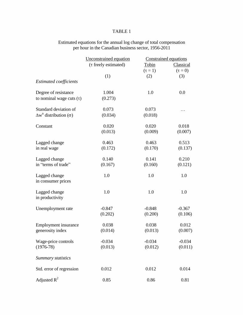
TABLE 1

Estimated equations for the annual log change of total compensation

per hour in the Canadian business sector, 1956-2011

Unconstrained equation Constrained equations

( freely estimated) Tobin Classical

( = 1) ( = 0)

(1) (2) (3)

Estimated coefficients

Degree of resistance 1.004 1.0 0.0

to nominal wage cuts () (0.273)

Standard deviation of 0.073 0.073 …

wn distribution () (0.034) (0.018)

Constant 0.020 0.020 0.018

(0.013) (0.009) (0.007)

Lagged change 0.463 0.463 0.513

in real wage (0.172) (0.170) (0.137)

Lagged change 0.140 0.141 0.210

in “terms of trade” (0.167) (0.160) (0.121)

Lagged change 1.0 1.0 1.0

in consumer prices

Lagged change 1.0 1.0 1.0

in productivity

Unemployment rate -0.847 -0.848 -0.367

(0.202) (0.200) (0.106)

Employment insurance 0.038 0.038 0.012

generosity index (0.014) (0.013) (0.007)

Wage-price controls -0.034 -0.034 -0.034

(1976-78) (0.013) (0.012) (0.011)

Summary statistics

Std. error of regression 0.012 0.012 0.014

Adjusted R2 0.85 0.86 0.81

TABLE 1 (continued)



( = 1) ( = 0)

(1) (2) (3)

P-values for residual tests

Breusch-Godfrey 3-lag 0.28 0.28 0.86

serial correlation LM test

Breusch-Pagan test 0.44 0.44 0.47

of heteroscedasticity

Jarque-Bera test 0.29 0.29 0.60

of normality of errors

P-values for coefficient tests

H0: impact of lagged consumer 0.66 0.68 0.001

price inflation is equal to 1

H0: impact of lagged change 0.89 0.89 0.33

in productivity is equal to 1

H0: full resistance to 0.99 … …

nominal wage cuts ( = 1)

H0: no resistance to 0.0006 … …

nominal wage cuts ( = 0)

P-values for stability tests

H0: no change in coefficient of lagged 0.43 0.42 0.80

consumer price inflation in 1992-2011

H0: no change in coefficient of 0.49 0.48 0.06

unemployment rate in 1992-2011

H0: estimate of is unchanged:

-- in 1992-2001 0.93 0.99 …

-- in 2002-2011 0.32 0.30 …

H0: linear trend for is insignificant:

-- from 1978 on 0.50 0.50 …

-- from 1991 on 0.42 0.41 …

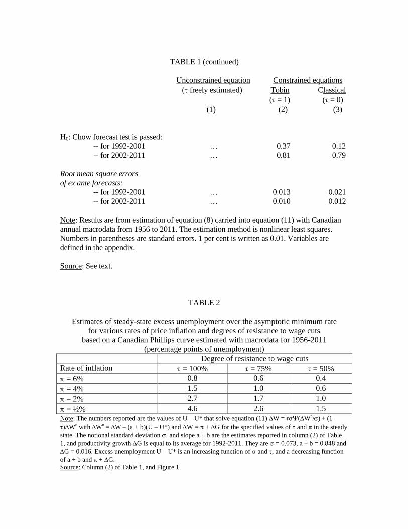
TABLE 1 (continued)



( = 1) ( = 0)

(1) (2) (3)

H0: Chow forecast test is passed:

-- for 1992-2001 … 0.37 0.12

-- for 2002-2011 … 0.81 0.79

Root mean square errors

of ex ante forecasts:

-- for 1992-2001 … 0.013 0.021

-- for 2002-2011 … 0.010 0.012

Note: Results are from estimation of equation (8) carried into equation (11) with Canadian

annual macrodata from 1956 to 2011. The estimation method is nonlinear least squares.

Numbers in parentheses are standard errors. 1 per cent is written as 0.01. Variables are

defined in the appendix.

Source: See text.

TABLE 2

Estimates of steady-state excess unemployment over the asymptotic minimum rate

for various rates of price inflation and degrees of resistance to wage cuts

based on a Canadian Phillips curve estimated with macrodata for 1956-2011

(percentage points of unemployment)

Degree of resistance to wage cuts

Rate of inflation = 100% = 75% = 50%

= 6% 0.8 0.6 0.4

= 4% 1.5 1.0 0.6

= 2% 2.7 1.7 1.0

= ½% 4.6 2.6 1.5

Note: The numbers reported are the values of U – U* that solve equation (11) W = (Wn/) + (1 –

)Wn with W

n = W – (a + b)(U – U*) and W = + G for the specified values of and in the steady

state. The notional standard deviation and slope a + b are the estimates reported in column (2) of Table

1, and productivity growth G is equal to its average for 1992-2011. They are = 0.073, a + b = 0.848 and

G = 0.016. Excess unemployment U – U* is an increasing function of and , and a decreasing function

of a + b and + G.

Source: Column (2) of Table 1, and Figure 1.

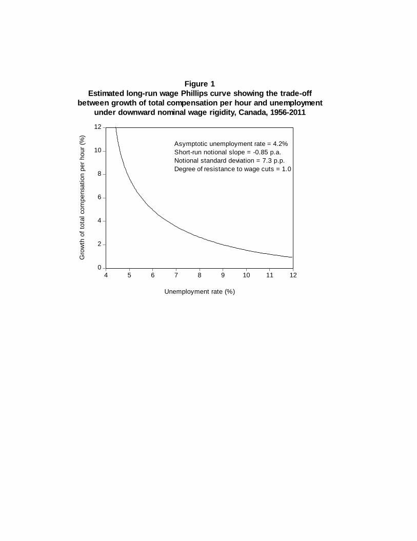
0

2

4

6

8

10

12

4 5 6 7 8 9 10 11 12

Unemployment rate (%)

Gro

wth

of

tota

l com

pen

satio

n p

er

hour

(%)

Figure 1

Estimated long-run wage Phillips curve showing the trade-off

between growth of total compensation per hour and unemployment

under downward nominal wage rigidity, Canada, 1956-2011

Asymptotic unemployment rate = 4.2%

Short-run notional slope = -0.85 p.a.

Notional standard deviation = 7.3 p.p.

Degree of resistance to wage cuts = 1.0

Documents

The Macroeconomics of Downward Nominal Wage … · period 1956-2011. This evidence suggests that the real world is more Tobin-like than classical, implying that the permanent unemployment