The Making of Social DemocracyThe Economic and Electoral Consequences of

Norway’s 1936 Folk School Reform∗

Daron AcemogluDepartment of Economics, Massachusetts Institute of Technology and NBER

Tuomas PekkarinenVATT Institute for Economic Research and Department of Economics, Aalto University School of Business

Kjell G. SalvanesDepartment of Economics, Norwegian School of Economics

Matti SarvimäkiDepartment of Economics, Aalto University School of Business; VATT and Helsinki GSE

July 22, 2021

Abstract

Upon assuming power for the first time in 1935, the Norwegian Labour Party deliveredon its promise for a major schooling reform. The reform raised minimum instruction timein less developed rural areas and boosted the resources available to rural schools, reducingclass size and increasing teacher salaries. We document that cohorts more intensively affectedby the reform significantly increased their education and experienced higher labor income.Our main result is that the schooling reform also substantially increased support for the Nor-wegian Labour Party in subsequent elections. This additional support persisted for severaldecades and was pivotal in maintaining support for the social democratic coalition in Norway.These results are not driven by the direct impact of education and are not explained by higherturnout, or greater attention or resources from the Labour Party targeted towards the munici-palities most affected by the reform. Rather, our evidence suggests that cohorts that benefitedfrom the schooling reform, and their parents, rewarded the party for delivering a major reformthat was beneficial to them.

Keywords: education, human capital, labor, schooling reform, social democracy, voting.JEL Classification: P16, I28, J26.

∗We are grateful to Ran Abramitzky, Jon Fiva, Matti Mitrunen, Karl Ove Moene, Bjarne Strøm, Janne Tukiainen,and numerous seminar participants for their comments and suggestions. We gratefully acknowledge financial supportfrom the Academy of Finland and the Norwegian Research Council.

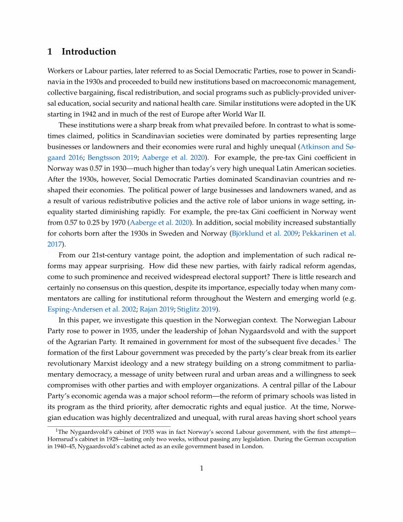
1 Introduction

Workers or Labour parties, later referred to as Social Democratic Parties, rose to power in Scandi-navia in the 1930s and proceeded to build new institutions based on macroeconomic management,collective bargaining, fiscal redistribution, and social programs such as publicly-provided univer-sal education, social security and national health care. Similar institutions were adopted in the UKstarting in 1942 and in much of the rest of Europe after World War II.

These institutions were a sharp break from what prevailed before. In contrast to what is some-times claimed, politics in Scandinavian societies were dominated by parties representing largebusinesses or landowners and their economies were rural and highly unequal (Atkinson and Sø-gaard 2016; Bengtsson 2019; Aaberge et al. 2020). For example, the pre-tax Gini coefficient inNorway was 0.57 in 1930—much higher than today’s very high unequal Latin American societies.After the 1930s, however, Social Democratic Parties dominated Scandinavian countries and re-shaped their economies. The political power of large businesses and landowners waned, and asa result of various redistributive policies and the active role of labor unions in wage setting, in-equality started diminishing rapidly. For example, the pre-tax Gini coefficient in Norway wentfrom 0.57 to 0.25 by 1970 (Aaberge et al. 2020). In addition, social mobility increased substantiallyfor cohorts born after the 1930s in Sweden and Norway (Björklund et al. 2009; Pekkarinen et al.2017).

From our 21st-century vantage point, the adoption and implementation of such radical re-forms may appear surprising. How did these new parties, with fairly radical reform agendas,come to such prominence and received widespread electoral support? There is little research andcertainly no consensus on this question, despite its importance, especially today when many com-mentators are calling for institutional reform throughout the Western and emerging world (e.g.Esping-Andersen et al. 2002; Rajan 2019; Stiglitz 2019).

In this paper, we investigate this question in the Norwegian context. The Norwegian LabourParty rose to power in 1935, under the leadership of Johan Nygaardsvold and with the supportof the Agrarian Party. It remained in government for most of the subsequent five decades.1 Theformation of the first Labour government was preceded by the party’s clear break from its earlierrevolutionary Marxist ideology and a new strategy building on a strong commitment to parlia-mentary democracy, a message of unity between rural and urban areas and a willingness to seekcompromises with other parties and with employer organizations. A central pillar of the LabourParty’s economic agenda was a major school reform—the reform of primary schools was listed inits program as the third priority, after democratic rights and equal justice. At the time, Norwe-gian education was highly decentralized and unequal, with rural areas having short school years

1The Nygaardsvold’s cabinet of 1935 was in fact Norway’s second Labour government, with the first attempt—Hornsrud’s cabinet in 1928—lasting only two weeks, without passing any legislation. During the German occupationin 1940–45, Nygaardsvold’s cabinet acted as an exile government based in London.

1

and limited school resources. The Labour Party promised to harmonize education and to increaseschool quality and instruction time in rural areas. As its first major reform, the new governmentlaunched an ambitious education reform, the Folk School Law of 1936, which increased fundingand resources, reduced class-size, expanded minimum instruction time and raised teacher salariesfor rural schools.2

Although sometimes overlooked in the historical work on the Scandinavian labor movement,education was a key pillar of social democratic agenda not just in Norway. The aim of the move-ment was to achieve greater social equality, and education was seen as an important tool for alter-ing the distribution of opportunities (Rothstein 1998). It was envisaged that the initial conditionsfor individuals would be made more equal with the help of state intervention in education or, asformulated by Lewin (1967), "the coercive power of the state". In Sweden, for example, leadingsocial democrats such as Tage Erlander, Olof Palme and Alva Myrdal were deeply involved in theplanning and implementation of education policy. Indeed, Myrdal saw the education policy as"the primary strategic instrument for abolishing class barriers" (Rothstein 1998).

We find that the 1936 education reform in Norway had distinct economic and political effects.We first show that years of education increased among the birth cohorts of boys living in areasmost affected by the reform exactly at the time when the reform started to affect these cohorts.Importantly, the reform did not alter years of mandatory education nor the provision of non-mandatory education. Thus these results likely reflect better preparedness for further education.We also estimate a positive effect on earnings in later life. For women, we do not find a statis-tically significant effect on post-mandatory education but—consistent with improved quality ofprimary education having direct labor market returns—there is a strong impact on their later in-come. Furthermore, our findings suggest that the reform may have had major intergenerationaleffects, although many of these estimates are not statistically significant due to our research de-sign’s relatively low statistical power for intergenerational analysis.

Our main focus is not the effects of the reform on education or earnings, but on Norwegianinstitutions and politics. We show that the reform was critical for the support for the LabourParty in subsequent elections in rural and less-developed parts of Norway. Before the reform, theLabour Party had less support in rural municipalities than urban areas. After 1936, however, itsvote share increased substantially in the more affected rural municipalities. These effects persistedfor at least two decades and are robust to controlling for region and pre-reform industry structureand average income. A back-of-an-envelope calculation suggests that the increase in the vote shareof the Labour Party in rural areas would have been 1.4–4.6 percentage points lower in 1945 if thereform had not taken place. The increase in rural support—a total of 3.9 percentage points—wascritical for the party, since in the meantime it lost 3.8 percentage points of its support in the cities.

2The other Nordic (Denmark, Sweden plus Finland) countries initiated and established similar school reforms forthe rural and urban areas following the Norwegian reform (Mediås 2004).

2

As a consequence, the traditionally higher support the Labour Party enjoyed in cities disappearedand the party has since been equally popular in rural and urban areas.

In the last part of this paper, we examine the mechanisms behind the impact of the reformon the Labour Party’s electoral success. We show that it is not because of a “direct educationeffect”—whereby the educated are more likely to be Labour Party supporters. In fact, during thisperiod, highly-educated Norwegians were more likely to vote for the more conservative parties.In addition, the electoral effect is largest in the first elections held after the reform, when most ofthe individuals directly affected by the reform were not yet eligible to vote. We also show thatthe Labour Party did not increase its electoral success because of increased political participationin the form of higher turnout (which was already very high in Norway at this time) or because itdevoted greater attention or resources to the municipalities most affected by the reform.

Rather, we argue our results are explained by the fact that the 1936 education reform was amajor promise of the Labour Party and a central pillar of its program for helping the less advan-taged parts of the country. The party delivered on its promise of major educational reform, andvoters rewarded it with lasting electoral support—especially by broadening the social democraticcoalition with the addition of previously-more conservative rural voters.

We provide four pieces of evidence consistent with this interpretation. First, we find that theelectoral effect is largely driven by municipalities that had not been previously exposed to Labourrule at local level, indicating a switch from conservative to Labour politics in places that bene-fited from the education reform. Second, using individual-level survey data collected from 1957parliamentary elections, we find that voters who themselves had experienced increased schoolingand improved school quality were much more likely to support the Labour Party. Third, ruralNorwegians with children born into the cohorts who had benefited from the 1936 school reformwere also much more likely to support the Labour Party than individuals with somewhat olderchildren (so that it was not just those receiving the education, but their entire family becomingmore pro-Labour). Fourth, in the same survey more than 90% of the respondents agreed that theNorwegian Labour Party had been willing and able to implement its agenda and those directlyaffected, and their parents, were particularly likely to hold this view.

Our methodology does not distinguish whether voters updated their beliefs about the com-petency of the Labour Party or felt indebted to the Labour Party.3 Nevertheless, the evidence isfairly clear that both inhabitants who benefited from the school reform and their parents were

3Greater support for a party that has kept its promises and delivered public goods is consistent with several mech-anisms. In addition to a change in beliefs about the “type” of the party, it could be because of standard retrospectivevoting (e.g., Ferejohn 1986; Persson et al. 2000) or because voters feel reciprocal altruism towards the party. Each ofthese mechanisms can be seen in functioning democracies but have also been at times associated with clientelistic orpopulist policies (e.g., Acemoglu et al. (2013) on the belief channel, Caprettini et al. (2021) on retrospective voting,and Finan and Schechter (2012) on reciprocal altruism). We suspect that the reason why the school reform in Norwaycontributed to the formation of a social democratic coalition, rather than any type of clientelistic political dynamics, isboth because of the broad-based nature of the policy in question and the efforts of the Labour Party to build a diversecoalition in support of its agenda.

3

much more likely to vote for the Norwegian Labour Party than other rural residents and thusprovided the popular support for the Social Democratic institutions in Norway.

This paper is related to a number of literatures. First, there is by now a large number of papersin labor economics evaluating the effects of various schooling reforms, ranging from compulsoryschooling and child labor laws to school building programs (e.g., Acemoglu and Angrist, 2000,Duflo, 2001, Black et al., 2005, Meghir and Palme, 2005, Oreopoulos, 2006, Pekkarinen et al., 2009;see Oreopoulos and Salvanes, 2011, for a review). To the best of our knowledge, none of theseworks investigate the political implications of these reforms.

Second and more directly, we contribute to the literature on the origins of social democracyin Scandinavia and Europe. Classic works in this area, such as Korpi (1983), Esping-Andersen(1990), Baldwin (1990) and Rothstein (1998), emphasize the role of labor unions and workers,though the central contribution of the coalition with agrarian interests has also received attention(e.g., Gourevitch 1986; Berman 2006). These emphases are different from but complementary toours, since many of these authors also recognize the importance of the public services providedby the Social Democratic parties.

Third, our paper relates to the literature on successful political reforms. In the context of demo-cratic reforms, Acemoglu and Robinson (2006, 2012) emphasize the role of collective action bypolitically excluded groups to force a transition away from non-democratic regimes, but also theimportance of fiscal redistribution, limited inequality and broad coalitions in order to ensure theconsolidation of new democratic regimes. Fearon (2011) and Bidner and François (2013) explorethe role of political accountability, bolstered by electoral institutions and collective action by cit-izens. Brender and Drazen (2007) explore the role of fiscal policies to reduce the fragility of newdemocracies. Giavazzi and Tabellini (2005) empirically investigate whether economic or politi-cal reforms come first in cross-country data. There is less systematic work on major institutionalreforms within democratic political systems. Fernandez and Rodrik (1991) and Strulovici (2010)propose theoretical arguments for why economic reforms in democratic societies will be delayedor blocked, and the literature on special interest politics, e.g., Grossman and Helpman (2001), alsooffers various reasons for inefficient reforms. We are not aware of theoretical or empirical work ineconomics or political science that investigates the impact of major school reforms on the politicalequilibrium. Consistent with this result, recent work by Acemoglu et al. (2021) finds that cohortsthat have lived longer under democracy, especially when a democracy is economically successfuland delivers public goods, tend to support democratic institutions and oppose non-democraticrule.

Fourth, many scholars have argued that education may increase support for democracy orcertain types of institutions (e.g., Verba and Almond 1963; Lipset 1959). More recently, Glaeseret al. (2007) claim to find support for this hypothesis, though more systematic analysis in Ace-moglu et al. (2005, 2008) show no impact of education or income on democracy, and points out

4

the problems in their empirical study. Milligan et al. (2004) show that educated individuals aremore likely to vote, but as pointed out in Friedman et al. (2016), this does not necessarily meanmore pro-democracy behavior in general. These authors show that disadvantaged Kenyans whoreceived more education because of schooling reform may have actually increased their supportfor political violence. Our work is very different from this literature, however, since we are notclaiming that education effects support for democracy or social democracy, but that education re-forms, which were the main electoral promise of the Labour Party before their 1936 victory, madeNorwegians more trusting and supportive of this party and their social democratic agenda.

The rest of the paper is organized as follows. In the next section, we provide the institutionalbackground for Norway in the 1930s, outline the state of education and describe the NorwegianLabour Party’s policy platform and the schooling reform it implemented upon assuming power in1935. Section 3 describes our data sources, while Section 4 outlines our empirical approach. Ourmain results are presented in Section 5. Section 6 explores the mechanisms behind the growth inthe support for Labour Party in areas and among cohorts benefiting from the schooling reform.Section 7 concludes, while the Appendix contains additional empirical results.

2 Norway’s Labour Movement and Educational Policy

The roots of the Scandinavian welfare state models can be traced back to the policies of centre-left governments that rose to power in between the world wars.4 Several liberal governmentsintroduced major labor laws, covering workers in the developing manufacturing sector from 1900until the end of the First World War. However, these laws did not enact universal policies, whichbecame to be a defining characteristic of the Nordic welfare states (Bull 1959; Bjørnson 2001).

Social democrats formed durable governments during the 1930s, typically in coalition withparties representing rural voters. The policies of these governments laid the foundations of thewelfare institutions that the same political forces continued to build after the WWII. These poli-cies included establishment of old age and disability pension, sickness leave, and unemploymentinsurance as well as large public investments in health and education. Norway followed this trendin 1935 when the Norwegian Labour Party formed a government with the support of the AgrarianParty.

2.1 Norway in the 1930s

Unlike what is sometimes claimed, the Nordic welfare states are not rooted in some underlyingstructural equality and consensus that predates the modern welfare state institutions. Quite thecontrary, before the 1930s Norway, like all the Nordic countries, was a highly unequal country with

4The Finnish welfare state, though ultimately ending up similar to the Scandinavian model, followed a differentpath owing to the disruptive effects of the 1918 civil war; see Meriläinen et al. (2020).

5

high levels of industrial conflict (Moene and Wallerstein 2006). In 1930, the Gini index in Norwaywas higher than the current Anglo-Saxon levels at 0.57 and the top 10 % share of the nationalincome was similar to the contemporaneous level in the United States at 0.44 (Aaberge et al. 2020).The regional inequalities were also striking, especially along rural-urban axis. According to Falkand Tovmo (2000), the gap in income per capita between the poorest municipality and the richestcity was 1 to 18 in 1930.

Although rapid structural change had already started by this point, almost 30% of the laborforce still worked in agriculture, and 45% of the population lived in urban areas. The Norwegianeconomy had been severely impacted by the postwar recession in Europe in the early 1920s, anddid not reach sustained recovery before it was hit again by the Great Depression in 1930. Due to thecombination of deflationary policies and external shocks, the GDP per capita grew only by 2.3%between 1919 and 1930 whereas the rest of the Scandinavian countries experienced solid growth,ranging from 23.5% in Sweden to 28.3% in Denmark during the same period. The poor growthperformance was reflected in high unemployment rate which never dropped below 9–10% duringthe 1920s and reached 33% in 1933. Norwegian labor markets were also affected by high levels ofindustrial conflict. According to Moene and Wallerstein (2006), the number of working days lostdue to strikes and lockouts in 1931 alone was three times larger than than the total amount of dayslost during the 25-year period between 1945 and 1970.

2.2 The Norwegian Labour Party

The development of the Norwegian labor movement followed the same broad pattern as simi-lar parties in Northern Europe, and in particular in other Scandinavian countries, although thereare also some distinct characteristics (Bull 1959; Esping-Andersen 1985; Sejersted 2011). The Nor-wegian Labour Party was founded in 1887 and entered the parliament in 1904. Its early historywas characterized by internal conflicts between the revolutionary and reformist factions. Untilthe 1930s, the party programs had a clear Marxist tone and an ambivalent attitude towards parlia-mentary democracy. Unlike the other Scandinavian Labour parties, Norwegian Labour Party wasalso a member of the Soviet led Comintern until the early 1920s.5

Following the poor performance in the 1930 election, the Norwegian Labour Party changed itsstrategy and adopted a reformist agenda following the example of its sister parties in Denmark,Germany, and Sweden (Bull 1959; Esping-Andersen 1985). This shift was also motivated by thepurges in the Soviet Union, the economic crisis which had severely affected the workers in in-dustrial, logging and fishing industries, and the threat of fascism which was gaining support in

5The reasons for the radicalization of the Social Democracy in Norway—contrasting with the experiences in Den-mark and Sweden—are not well understood. One hypothesis is that it is rooted in the age composition of the industrialworkforce in Norway, where the relatively late industrialization, taking off only between 1905 and 1910, meant thatworkers were much younger and perhaps more willing to support radical politics (Dahl 1971).

6

Norway (led by the now infamous Vidkun Quisling).The new strategy was built on three pillars. First, together with the main trade union, the

Labour Party established a more cooperative approach towards the employer organizations andmanaged to compel the employer organizations to recognize the National Confederation of Work-ers (LO) as a negotiating partner.6 The party also shifted its economic policy by adopting a Keyne-sian program of stabilization policy following an influential pamphlet "a 3-year plan for Norway"(En norsk 3-års plan) by Ole Colbjørnsen and Axel Sømme. Second, the Labour Party moved fromits earlier focus on industrial workers to a message of unity between rural and urban areas as wellas owners of small business and part of the educated middle-class such as teachers and public sec-tor workers (see Appendix Figure A1 for an illustration of this change between the 1930 and 1933election campaigns). Third, the party made a clear break with revolutionary Marxist ideology andfully committed to advance its reformist agenda through parliamentary democracy and allianceswith other parties.

These changes made the Norwegian Labour Party more appealing to moderate voters andmore acceptable as a coalition partner for centerist parties. In the 1933 election, the party increasedits vote share from 31% to 40%, the highest share it had ever gained. Although the electioral succesdid not immediately lead to the formation of a Labour government, the minority government ledby the Liberal Party collapsed in 1935, when the Agrarian Party withdrew its support and agreedto support the Labour minority government with Johan Nygaarsdvold as its prime minister.

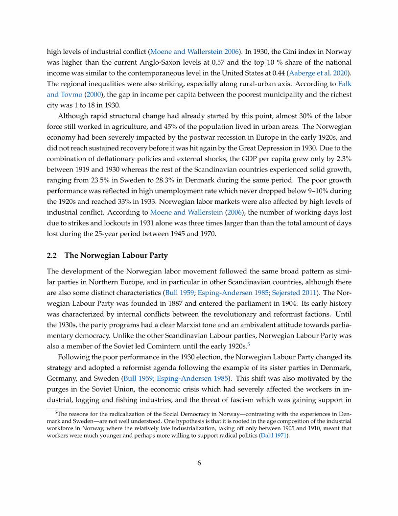
The 1935 Labour government started a long period of social democratic rule. As show in Fig-ure 1, the Labour Party held power for most of the following 45 years apart from the Germanoccupation in 1940–1945 (when the Labour government was in exile in London) and short periodsof center-right governments in the 1960s and 1970s. During this long period, the Labour Partyimplemented an ambitious program for developing the welfare state that included the introduc-tion of universal national social security, health care system, and, later, day care and family leavepolices.

2.3 Primary education in Norway before 1935

The Norwegian legislation on primary schools dates back to the 18th century. The first Law ofPrimary education for the Kingdom of Denmark-Norway was introduced in 1739. Education wasthe responsibility of the church until 1840s, when regional federalism was introduced and theresponsibility of organizing primary education was delegated to municipalities. In 1861, the focusof primary schooling was changed from preparing children for confirmation at the age of 15 to

6This agreement was made just before the formation of the Labour government in 1935. It resembled the Saltsjøbadagreement of 1938 in Sweden and the agreements established already around the turn of the century in Denmark.The new national rules for wage negotiations were also signed by the National Confederation of Employers (NAF)and the National Confederation Workers. After WWII, the government also started to take an active part in the wagenegotiations as a third party.

7

Figure 1: Labour party’s election results and periods in government, 1905–1981

inexile in government

seat share

vote share

revolutionary reformist

0

.1

.2

.3

.4

.5

.6

19061909

19121915

19181921

19241927

19301933

19361945

19491953

19571961

19651969

19731977

1981

Note: This figure reports the vote shares of the Norwegian Labour Party in parliamentary elections and the share ofseats the party held in the parliament. The gray areas present the periods, when the Labour party was in government,and the red area the period that the Labour government spent in exile in London following the Nazi occupation. Thechange in the link between vote and seat shares in 1921 is due to a move to a proportional representation. The drop inthe vote share in 1921–1924 is due to the temporary split of the party into the Social Democratic Party of Norway andNorwegian Labour Party, see Cox et al. (2019) for details.

preparing children in general including algebra in addition to reading and writing.Because the demand for primary education was understood to be lower in the rural areas

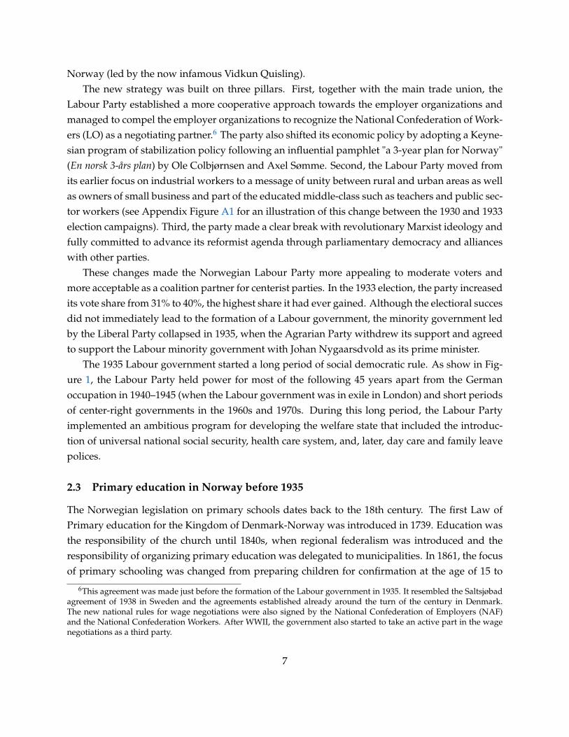
and in fishing communities—sectors that were also exempt from the child labor laws—the lawon primary schools stipulated shorter school years for rural than for urban areas, in particular,with lower minimum and maximum number of school weeks in rural parts. Even though theschool weeks included slightly more hours in rural areas, the restrictions on the number of weeksimplied that rural primary school students received substantially less instruction time than theirurban counterparts. As shown in Figure 2, the requirement in 1928 was that rural schools hadto provide just 3,096 hours of education over seven years of mandatory education, whereas thecorresponding figure was 4,912 hours in urban areas. In addition, the content of education variedwidely across municipalities as the law on primary schools did not establish guidelines about thenumber of hours allocated to different subjects.

The differences in instruction time between rural and urban areas were considered a problemfrom early on. The law was revised in 1915, when the minimum number of weeks of instructiontime in the last four primary school grades was increased to 14 weeks.7 However, the differences

7The 1915 law increased the number of minimum and maximum hours of instruction time in rural schools by 11%and 40%, respectively

8

Figure 2: Minimum cumulative hours in rural and urban primary schools, 1889–1959

Folk SchoolReform

Comprehensive SchoolReform

0

1000

2000

3000

4000

5000

6000

Cum

ulat

ive

hour

s

1889 1915 1927 1936 1955 1959

Rural Urban

Note: This figure reports minimum cumulative hours over seven years of mandatory education in rural and urbanareas. Source: Norwegian Parliament Besl. O. No. 35, May 15th 1889; Besl. O. No. 36, May 28th 1889; Besl. O. No. 112,June 23rd 1915; Besl. O. No. 27, March 17th 1928; Besl. O. No. 114, June 7th 1936; Lov om folkeskulen pålandet Jun16th, 1936.

in the standards and the quantity of primary school education were exacerbated during the eco-nomic crises in the 1920s. As education was mostly locally funded, variation in the local economicconditions meant that the municipal authorities’ ability to invest in primary education began todiverge. In 1935, urban areas provided 211 days of primary education, on average, while theaverage in rural areas was only 89.

2.4 Education policy in the Labour Party programs

Although often overlooked in the historical work on the Nordic labor movement, education pol-icy was regarded as a key component in the political model for social change by the early socialdemocrats. The aim of the movement was to achieve greater social equality, for which educationwas going to be a critical tool as it would alter the distribution of opportunities (Rothstein 1998).The initial conditions for individuals would be made more equal with the help of state interven-tion in education or, as formulated by Lewin (1967): "the coercive power of the state". The primacyof educational policy was reflected in the fact that, in the Swedish case, many of the leading socialdemocratic politicians and strategists, such as Tage Erlander, Olof Palme, and Alva Myrdal, weredeeply involved in the planning and implementation of education policy from early on. Indeed,Myrdal saw the education policy as "the primary strategic instrument for abolishing class barriers"(Rothstein 1998).

The importance of the education reform is very clear in the party programs of the Norwegian

9

Labour Party. Already the very first program from 1885 called for "free and general education instate schools". These demands became more specific over time and clear emphasis was put onequal opportunities for children in different parts of Norway. Already in 1903, the party calledfor general primary school "for all children in the society", for "increase in the minimum hours ofinstruction", and that "the country side primary schools should be brought to the same level asthe town primary schools". By 1930s, the urgency of the education reform was so clear that the1936 program listed it as the third objective after democratic rights and equal justice. Accordingto the program "primary schools should be turned into a general comprehensive school that pre-pares children for further education." The party called for the central government to take over thefinancing of the schools and repeated the demand for the equal quality of primary schools andincreased instruction time across the country.

2.5 The 1936 Folk School Law for Rural Areas

The Norwegian Labour Party’s conviction that the country’s education system was unequal andill-suited for the demands of a rapidly changing economy shaped its reform priorities. To addressthe foundational problem of lack of equal access to primary education of sufficiently high quality,the new Labour government passed the new law on primary schools in rural areas as one of itsfirst major pieces of legislation in 1936. This reform was the first step in a program that aimed atestablishing a general comprehensive primary school which would prepare children for furthereducation (Rust 1989).8

The new law on primary schools increased the minimum instruction time in rural areas to 16weeks for the first three years of primary education and 18 weeks for the the subsequent fouryears. In addition to these changes, the law decreased the maximum class size from 35 to 30. Thefunding from the central government was increased to cover a larger share of the base salariesof teachers and provided funding to pay teachers age and region related bonuses.9 The statealso took over other responsibilities that were previously carried out by the municipalities, sucha school buildings, books and inventories, as well as housing for the teachers. Furthermore, anew national curriculum was introduced ("Normalplanen for Folkeskolen" from 1939) with a focuson skills rather than religious education and a ban on physical punishment. The new curriculumreduced the regional variation in the content of education (Rust 1989).10

The reform was a compromise, and the Labour Party decided not to advance some of its long-term goals like removing religious education from schools. Nevertheless, the goals of the 1936reform were ambitious, considering the state of primary schools in rural municipalities in the

8Establishing a comprehensive school had been suggested by several "school commissions" from early-1900s on-wards, but never gained enough support in the Parliament. Even as late as in 1934 extensions of increased hours inrural schools was voted down with support from conservatives as well as the agrarian party.

9The law increased the share of central government funding from 45% of minimum teacher salary to 50%.10See also Chapter 5 of "Lov om folkeskolen på landet", 1936.

10

mid-1930s. Only 4% of the rural municipalities were providing more than 16 weeks of instructionin lower classes of primary schools in 1935. The percentage of municipalities fulfilling the criteriaof the new law in higher grades was similarly small at 4%, and a mere 2% of the municipalitiesmet the new requirements in all primary school grades. Thus, the new legislation forced a vastmajority of rural municipalities to increase instruction time. The requirement on the maximumclass size was also binding for most municipalities, with only 40% of municipalities meeting therequirements of the old law that there should be a maximum of 35 students per teacher. Just 22%had classes smaller than the new requirement of 30 students per teacher.

The law was passed swiftly and and came into force from the school year starting in August1936. Municipalities were allowed to use five years to implement it fully. Hence, children bornin 1935, and consequently starting school in August 1942, are the first cohort for whom the newregime was fully implemented.

3 Data

We created our main data set by linking together newly digitalized archival data on the roll out ofthe 1936 primary school reform, individual-level population-wide information on human capitaland income, and municipality-level data on election results and pre-reform characteristics. Inorder to explore mechanisms, we also use survey data from 1957 on political preferences and dataon candidate characteristics in national elections from Fiva and Smith (2017). We next describeeach of these data sources in more detail.

3.1 Schools

We create our treatment variable, discussed in detail in the next section, using municipality-levelinformation on the provision of primary education, which we collected from Norwegian archivesand digitized. These data originate from county-level primary school directors, who were obligedto send a report every year to Statistics Norway. The information content of the data varies byyear, but we can form a time-series for each municipality on the average weeks of school by gradefrom the 1920s onwards. For some years, we also observe the within-municipality distributionof children by weeks of education, the extent to which several grades were taught in the sameclass, the gender composition, education and compensation of the teachers, and the type of schoolbuildings available.11

11Detailed description and aggregated data are available at https://www.ssb.no/a/histstat/publikasjoner/histemne-21.html.

11

3.2 Human capital and income

We link the municipality-level measures of primary education to individual-level data using infor-mation on individuals’ municipality of birth. Our individual-level data contain population-wideinformation about educational attainment, earnings, demographics, and family links. In addition,we observe information from military records for a subsample of men.

We conduct separate analyses for two groups. The “first-generation” consists of individualsborn in rural Norwegian municipalities in 1917–1940. Second, we define the “second-generation”as the children of the first-generation (regardless of their own place of birth), and restrict theanalysis to those born in 1947–1976. We do not impose any further sample restrictions, althoughsome individuals with missing information naturally drop out of our sample.

We use completed years of education as our primary measure for human capital. This infor-mation is drawn from the 1960 and 1970 population censuses and Statistics Norway’s educationaldatabase and is thus available for the full population. For men serving the mandatory military ser-vice after 1969, we also observe IQ scores. Roughly 95% of Norwegian men in the relevant birthcohorts took arithmetics, vocabulary, and Raven Progressive Matrix tests at the age of 18–20 at thedraft board meeting for mandatory military service (see Sundet et al. 2004, for details). We use thecomposite score of these three tests as our second human capital measure. In addition, we observeannual income form 1969 onwards as recorded in the pension register. This income measure in-cludes labor earnings, taxable sick benefits, unemployment benefits, parental leave payments andpensions. We construct proxies for lifetime income using average income over ages 50–64 for thefirst-generation and average income over ages 30–34 for the second-generation.

Table 1 presents sample averages by treatment intensity (as defined in the next section) for ourmain estimation sample. On average, the first generation men have 9.0 and women 8.4 years ofeducation and almost half of them did not continue their education after leaving primary school.Men’s average annual income at ages 50–64 is 180,000 Norwegian kronas (in 1998 prices) cor-responding to about $21,000 (in 2020 prices). For women, the corresponding figures are 80,000kronas or $9,000. There is a clear, although relatively mild, gradient by treatment intensity withthose born in poorer (and thus more intensely treated) municipalities having somewhat less edu-cation and lower income than those born in municipalities less affected by the reform. As shownin the lower panel, the second-generation has more education and higher incomes than the first-generation, and part of the differences along the treatment intensity distribution are still present.

3.3 Election results and municipality characteristics

Our primary election measures are drawn from Municipality Data Base of The Norwegian Centerfor Research Data. These data provide municipality-level information on votes cast for the mainpolitical parties in national elections and on voter turnout. We complement these data with in-

12

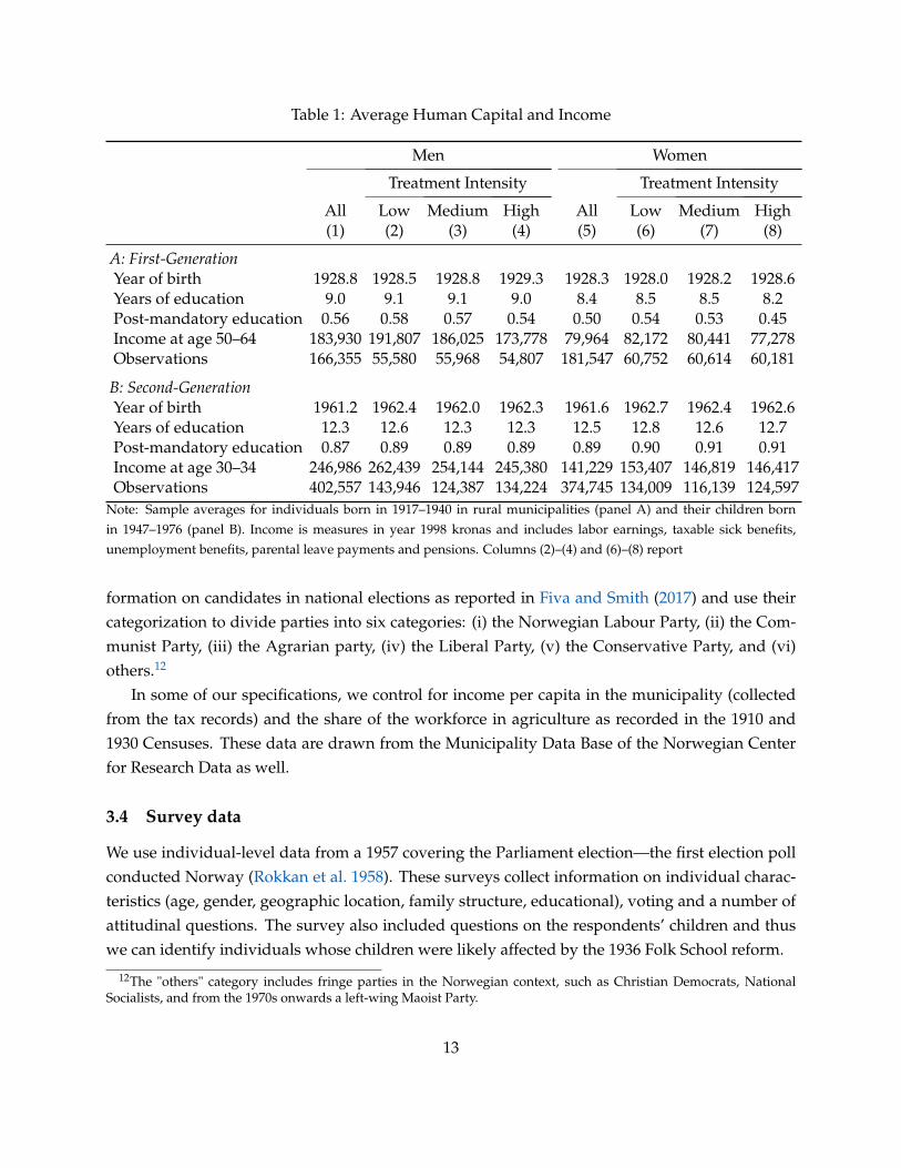
Table 1: Average Human Capital and Income

Men Women

Treatment Intensity Treatment Intensity

All Low Medium High All Low Medium High(1) (2) (3) (4) (5) (6) (7) (8)

A: First-GenerationYear of birth 1928.8 1928.5 1928.8 1929.3 1928.3 1928.0 1928.2 1928.6Years of education 9.0 9.1 9.1 9.0 8.4 8.5 8.5 8.2Post-mandatory education 0.56 0.58 0.57 0.54 0.50 0.54 0.53 0.45Income at age 50–64 183,930 191,807 186,025 173,778 79,964 82,172 80,441 77,278Observations 166,355 55,580 55,968 54,807 181,547 60,752 60,614 60,181

B: Second-GenerationYear of birth 1961.2 1962.4 1962.0 1962.3 1961.6 1962.7 1962.4 1962.6Years of education 12.3 12.6 12.3 12.3 12.5 12.8 12.6 12.7Post-mandatory education 0.87 0.89 0.89 0.89 0.89 0.90 0.91 0.91Income at age 30–34 246,986 262,439 254,144 245,380 141,229 153,407 146,819 146,417Observations 402,557 143,946 124,387 134,224 374,745 134,009 116,139 124,597

Note: Sample averages for individuals born in 1917–1940 in rural municipalities (panel A) and their children bornin 1947–1976 (panel B). Income is measures in year 1998 kronas and includes labor earnings, taxable sick benefits,unemployment benefits, parental leave payments and pensions. Columns (2)–(4) and (6)–(8) report

formation on candidates in national elections as reported in Fiva and Smith (2017) and use theircategorization to divide parties into six categories: (i) the Norwegian Labour Party, (ii) the Com-munist Party, (iii) the Agrarian party, (iv) the Liberal Party, (v) the Conservative Party, and (vi)others.12

In some of our specifications, we control for income per capita in the municipality (collectedfrom the tax records) and the share of the workforce in agriculture as recorded in the 1910 and1930 Censuses. These data are drawn from the Municipality Data Base of the Norwegian Centerfor Research Data as well.

3.4 Survey data

We use individual-level data from a 1957 covering the Parliament election—the first election pollconducted Norway (Rokkan et al. 1958). These surveys collect information on individual charac-teristics (age, gender, geographic location, family structure, educational), voting and a number ofattitudinal questions. The survey also included questions on the respondents’ children and thuswe can identify individuals whose children were likely affected by the 1936 Folk School reform.

12The "others" category includes fringe parties in the Norwegian context, such as Christian Democrats, NationalSocialists, and from the 1970s onwards a left-wing Maoist Party.

13

4 Empirical Approach

We follow an identification strategy similar to those used in Card (1992) and Acemoglu and John-son (2007). This approach builds on the notion that the reform mattered more for municipalitiesthat were further away from the new (national) standards and for the birth cohorts that spent alarger share of their primary education under the new regime. We next discuss how we measurethis treatment intensity and how we use it to estimate the impacts of the reform.

4.1 Treatment measures

Our identifying variation arises from two sources. First, the reform’s impact varied across mu-nicipalities because of cross-municipality differences in primary education provision before thereform. In particular, the reform had greater "bite" in municipalities that were far away from thepost-reform requirements. In contrast, it had little impact on municipalities that already met orexceeded the new requirements. We measure this distance to the post-reform minimum require-ments using information on instruction time just before the reform was passed. Specifically, weobserve the share of children by instruction time brackets separately for grades 1–3 and 4–7 foreach municipality in 1935 and summarize this information with a municipality-level index:

Zj =3 ∑b sbjmax (16 − b, 0) + 4 ∑b Sbjmax (18 − b, 0)

28, (1)

where sbj are the shares of children in grades 1–3 who received b weeks of education in munic-ipality j in 1935, and Sbj are similar shares for grades 4–7. The nominator captures the averageadditional weeks of instruction a municipality would have to offer in order to meet the new re-quirements.13 The denominator is a scaling factor corresponding to the cumulative change inminimum requirements induced by the reform (28 weeks over seven years of education). Thus,Zj takes the value of one for a municipality at the pre-reform minimum in 1935 and zero for amunicipality that already exceeded the new requirements before the reform.

The second source of identifying variation occurs between birth cohorts within a municipality.Those born before 1923 had left primary education by the beginning of the implementation periodin 1936 and thus were not exposed to the reform. On the other hand, everyone born after 1935started school after the implementation period and went through their entire primary educationunder the new requirements. Among the 1923–1935 birth cohorts, the treatment intensity dependson the year of birth, the year the municipality implemented the reform, the "bite" the reform (Zj),

13For example, think of a municipality, where half of the children in grades 1–3 got 12 weeks of education and theother half got 14 weeks of education in 1935. Let’s further assume that all 4–7th graders received 18 weeks of educationin 1935 in this municipality. Recall that the reform mandated that instruction time needed to be at least 16 weeks peryear for grades 1–3 and to 18 weeks per year for grades 4–7. Thus the reform induced 3× [0.5× (16− 12) + 0.5× (16−14)] = 9 weeks of additional education for an average child living in this municipality.

14

Figure 3: Treatment intensity

(a) Geographical distribution (b) Pre-reform income and industrial structure

.5

.55

.6

.65

.7

.75

.8

LFS

of a

gric

ultu

re a

nd fi

shin

g

8

9

10

11

12

13

14

15

16

Aver

age

inco

me

in 1

930

0.0 0.1 0.2 0.3 0.4 0.5 0.6 0.7 0.8 0.9 1.0 1.1Zj

Average income(left axis)Labor force sharein agriculture andfishing (right axis)

Note: Panel (a) presents the geographical distribution of the treatment intensity, Zj, see equation 1. Panel (b) shows theassociation between Zj and average income of municipalities.

and the extent to which the municipality complied with the new requirements.14

We combine these sources of variation as a municipality–birth cohort level measure

Zjc = ∑c

πcZj (2)

where πc is the share of years birth cohort c studied under the new requirements. We do notknow when each municipality implemented the reform. Thus, as a baseline, we assume that allmunicipalities fully implemented the reform in 1938, and set πc = 0 for everyone born in or before1924, πc = 1 for everyone born in or after 1931, and πc = (c − 1924)/7 for those born between1925 and 1930. We show that the results are robust to assuming other implementation years.

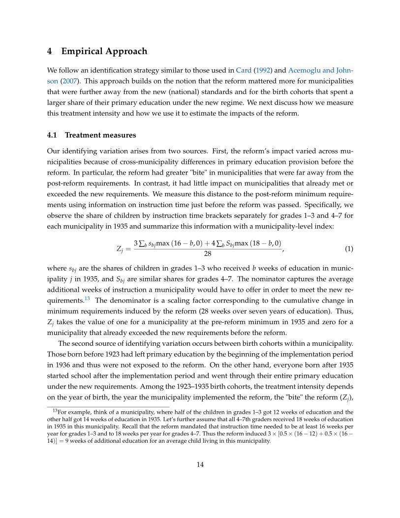
Having defined the treatment intensity measures, we next examine their geographical distri-bution and association with pre-reform municipality characteristics. Panel (a) of Figure 3 showsthat municipalities in the northern (less economically developed) parts of Norway tended to be

14For example, consider a municipality that followed the pre-reform minimum requirements before the reform andfully implemented the new requirements in 1938. In this case, children born in 1925 had started first grade at the ageof 7 in 1932 and attended only their final (seventh) grade under the new requirements in 1938. Those born in 1926attended school for two years after the reform, those born in 1927 for three years and so forth. Finally, everyone bornin or after 1931 received the full treatment.

15

further away from the post-reform minimums, and hence more affected by the reform, than thoselocated further to the south. However, there is also variation across the whole of Norway andsometimes large differences between neighboring municipalities. Nevertheless, as the reform wasdesigned to improve education in more deprived areas, treatment intensity is naturally associatedwith pre-reform municipality characteristics. Panel (b) of Figure 3 illustrates these differences byplotting municipalities’ average income and share of labor force working in agriculture and fish-ing in 1930 by deciles of Zj. It shows that municipalities that were providing the minimum (orless) pre-reform instruction time in 1935 (Zj ≥ 1) were substantially poorer and had a much largershare of the labor force working in the primary sector. These differences motivate the differences-in-differences approaches we next discuss.

4.2 Specifications

We start our analysis by asking how the reform affected human capital and income of the directlyaffected individuals and estimate event-study regressions of the form:

yicj = Zjβc + Xj0θc + µc + µj + εicj (3)

where yicj is the outcome of interest for individual i born in year c in municipality j.15 On theright-hand-side, Zj is the pre-reform distance from the new requirements (see equation (1)), Xj0 isa vector of municipality characteristics measured before the reform, µc is a vector of year of birthfixed effects, and µj is a vector of municipality of birth fixed effects.16 The parameters of interestare βc, which measure the extent to which the outcome grows differentially between birth cohortc and birth cohort 1923–24 (the omitted category) across municipalities that were differentiallyaffected by the reform.

We report estimates from several specifications that differ in terms of what is included in thevector Xj0. The specifications are motivated by the correlation between treatment intensity andpre-reform geographical location, income and industrial structure discussed above. While themunicipality fixed effects capture all time-invariant differences between municipalities, it is con-ceivable that poorer or less industrialized municipalities would have evolved differently than themore prosperous ones even in the absence of the reform. Hence, we examine alternative specifi-cations allowing for differential trends by geographical location, average income and industrialstructure.

The advantage of the event-study specification is that it allows us to examine whether thetiming of the possible changes is consistent with the timing of the reform. It also provides a

15We do not include a subscript for calendar year here because our individual-level measures consist of education,income and cognitive ability test scores, all recorded at a fixed age.

16Note that using municipality of birth and not municipality of residence helps reducing a potential bias due tomobility across municipalities.

16

falsification exercise for the parallel pre-trends assumption required for a causal interpretation ofβc. However, this flexibility comes with the cost of a large number of parameters. In order toefficiently summarize the results from the event-studies, we also estimate a more parsimoniousversion where we estimate a single parameter specifying the effect of all post-reform years:

yicj = βZjc + Xj0θc + µc + µj + εicj, (4)

where Zjc is the municipality–birth cohort level measure of treatment intensity (see equation (2))and other variable are as in the previous specification.

We analyze the impacts on electoral outcomes using a similar approach. However, here, wecannot utilize variation across birth cohorts, because electoral outcomes are available only at themunicipality–year level. Thus, we start with event-study specifications of the form:

yptj = Zjβt + Xj0θt + µt + µj + εptj (5)

where yptj is the vote share of party p in year t at municipality j, and Zj and Xj0 are the sametreatment intensity measure and pre-reform observable characteristics as above. The parametersof interest, βt, now measure the extent to which the vote share of a party increased faster betweenthe 1933 elections and elections in year t in municipalities more affected by the reform.

In order to increase statistical power and to summarize the estimates into a single number, wealso report estimates from a standard differences-in-differences specification:

yptj = β(1[t ≥ 1945]× Zj) + Xj0θt + µt + µj + εptj (6)

where 1[t ≥ 1945] is an indicator variable taking the value one for post-war years and zero forpre-war years, while other variables are as above.

We interpret all our estimates as the intention-to-treat effect of the reform. We note that ourmeasure of treatment intensity Zj is constructed using data on instruction time. An alternativeapproach would be to define the treatment as instruction time and use Zcj as and instrumentalvariable for it. We do not use this strategy because we believe the exclusion restriction necessaryfor such an IV approach is not valid. This exclusion restriction would require that the effects of thereform worked entirely via changes in instruction time, whereas, as is common with other educa-tion reforms, the Norwegian reform affected several dimensions of educational inputs at the sametime (see Section 2.5). Appendix Figure A2 illustrates this point by plotting average instructiontime and student-teacher ratio as functions of treatment intensity in years 1930, 1935, 1938 and1940-1944. It shows that the pre-reform values of all inputs were highly correlated with our treat-ment intensity variable, but this correlation clearly declines after the reform was implemented in1938, implying that the main dimensions of the reform were correlated with each other.

17

5 Results

This section presents our main results. We start by examining the impact of the reform on humancapital and long-term income of the individuals who were directly affected by it. This analysis ismotivated by the 1936 reform’s primary objective of harmonizing the standards of primary edu-cation across municipalities. Hence, if the reform was successful in increasing resources allocatedto primary education in the municipalities most affected by it, we would expect an increase inyears of education and in earnings. We find that this is, indeed, the case. We then show thatthe reform may have had an intergenerational effect also on human capital and earnings on thechildren of those directly affected, although these estimates are much less precise in some spec-ifications. Finally, we present our core results showing that the reform increased the vote shareof the Norwegian Labour Party in municipalities that were more affected by the reform. Theseeffects are present both in the short and in the long run and indicate that the reform played animportant role in closing the rural-urban gap in the support for the Norwegian Labour Party. Wereturn to the potential mechanisms behind these effects in the next section.

5.1 Direct impact on human capital and income

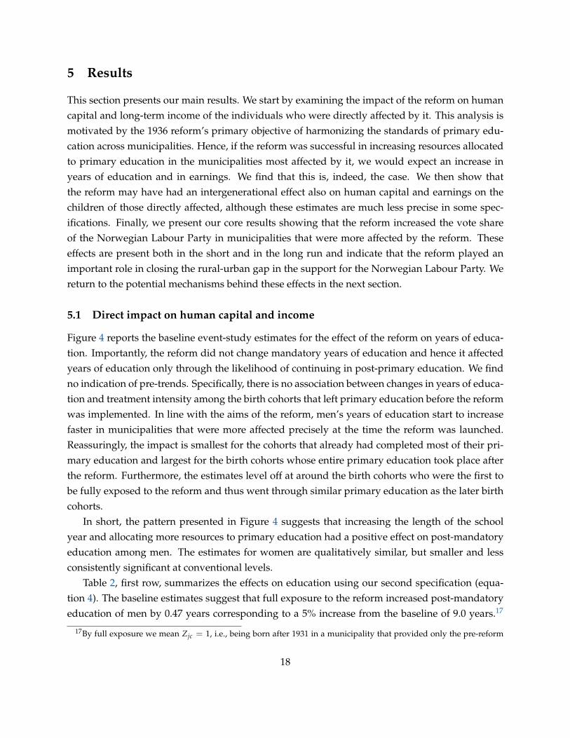
Figure 4 reports the baseline event-study estimates for the effect of the reform on years of educa-tion. Importantly, the reform did not change mandatory years of education and hence it affectedyears of education only through the likelihood of continuing in post-primary education. We findno indication of pre-trends. Specifically, there is no association between changes in years of educa-tion and treatment intensity among the birth cohorts that left primary education before the reformwas implemented. In line with the aims of the reform, men’s years of education start to increasefaster in municipalities that were more affected precisely at the time the reform was launched.Reassuringly, the impact is smallest for the cohorts that already had completed most of their pri-mary education and largest for the birth cohorts whose entire primary education took place afterthe reform. Furthermore, the estimates level off at around the birth cohorts who were the first tobe fully exposed to the reform and thus went through similar primary education as the later birthcohorts.

In short, the pattern presented in Figure 4 suggests that increasing the length of the schoolyear and allocating more resources to primary education had a positive effect on post-mandatoryeducation among men. The estimates for women are qualitatively similar, but smaller and lessconsistently significant at conventional levels.

Table 2, first row, summarizes the effects on education using our second specification (equa-tion 4). The baseline estimates suggest that full exposure to the reform increased post-mandatoryeducation of men by 0.47 years corresponding to a 5% increase from the baseline of 9.0 years.17

17By full exposure we mean Zjc = 1, i.e., being born after 1931 in a municipality that provided only the pre-reform

18

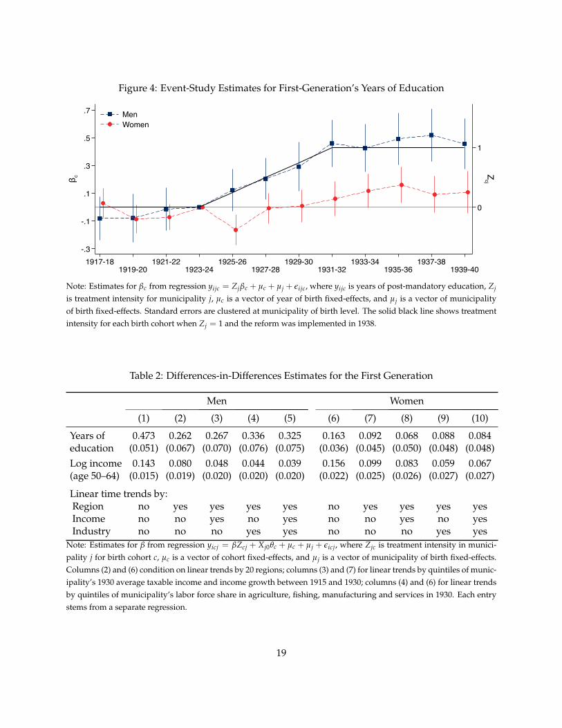
Figure 4: Event-Study Estimates for First-Generation’s Years of Education

0

1

Zcj

-.3

-.1

.1

.3

.5

.7

β c

1917-181919-20

1921-221923-24

1925-261927-28

1929-301931-32

1933-341935-36

1937-381939-40

MenWomen

Note: Estimates for βc from regression yijc = Zjβc + µc + µj + εijc, where yijc is years of post-mandatory education, Zj

is treatment intensity for municipality j, µc is a vector of year of birth fixed-effects, and µj is a vector of municipalityof birth fixed-effects. Standard errors are clustered at municipality of birth level. The solid black line shows treatmentintensity for each birth cohort when Zj = 1 and the reform was implemented in 1938.

Table 2: Differences-in-Differences Estimates for the First Generation

Men Women

(1) (2) (3) (4) (5) (6) (7) (8) (9) (10)

Years of 0.473 0.262 0.267 0.336 0.325 0.163 0.092 0.068 0.088 0.084education (0.051) (0.067) (0.070) (0.076) (0.075) (0.036) (0.045) (0.050) (0.048) (0.048)Log income 0.143 0.080 0.048 0.044 0.039 0.156 0.099 0.083 0.059 0.067(age 50–64) (0.015) (0.019) (0.020) (0.020) (0.020) (0.022) (0.025) (0.026) (0.027) (0.027)

Linear time trends by:Region no yes yes yes yes no yes yes yes yesIncome no no yes no yes no no yes no yesIndustry no no no yes yes no no no yes yes

Note: Estimates for β from regression yicj = βZcj + Xj0θc + µc + µj + εicj, where Zjc is treatment intensity in munici-pality j for birth cohort c, µc is a vector of cohort fixed-effects, and µj is a vector of municipality of birth fixed-effects.Columns (2) and (6) condition on linear trends by 20 regions; columns (3) and (7) for linear trends by quintiles of munic-ipality’s 1930 average taxable income and income growth between 1915 and 1930; columns (4) and (6) for linear trendsby quintiles of municipality’s labor force share in agriculture, fishing, manufacturing and services in 1930. Each entrystems from a separate regression.

19

For women, the point estimate suggest a 0.16 years or a 2% increase from the baseline of 8.2 years.Columns (2) and (6) report results from specifications that allow differential linear trends for eachof Norway’s 20 regions and hence control for overall regional convergence that may have beencorrelated with the reform. The estimates are now 0.26 years for men and 0.09 for women andremain statistically significant. In the rest of the table, we allow for differential linear trends by1930 average taxable income, changes in average taxable income between 1915 and 1930, and theindustrial structure of the municipality 1930 (see the table note for details). Appendix Figure A3presents the corresponding event-study estimates using the same control variables. The most de-manding specification allowing for differential trends by region, income and industry suggest thatfull exposure to the reform increased the post-mandatory education of men by 0.33 years (p-value<0.001) and that of women by 0.084 years (p-value 0.084).

The remaining of Table 2 repeats the analysis using average log income at ages 50–64 as anoutcome variable. The estimates are statistically and economically significant, but sensitive tocontrolling for differential trends by region or 1930 municipality characteristics. This sensitivitysuggests that average incomes in areas more affected by the reform converged towards incomesof other regions not just due to the effects of the reform on education. Most likely, there wouldhave been some amount of convergence even without the reform, and as a result, we also see asmall pre-trend among men in the baseline specification (Appendix Figure A4). Thus, the baselineestimates for men’s income are likely to be biased upwards. However, the estimates are relativelystable in specifications allowing for differential trends by region and either income or industrialstructure (or both). These most demanding specification suggests that a full exposure to the reformincreased long-term income of men by 3.9 log points (p-value 0.053) and that of women by 6.7 logpoints (p-value 0.013). Thus, we conclude that the reform’s impact was likely to increase long-termincome, although this evidence is somewhat less conclusive than in the case of years of education.The results for women also suggest that improved primary education was valuable in the labormarket even when it did not increase the likelihood of further education.

5.2 Intergenerational effects

In line with the Norwegian Labour Party’s objective of improving overall social mobility, we findevidence that the schooling reform also increased the educational attainment of the children ofcohorts directly impacted by the reform.

Figure 5 presents event-study estimates for the second-generation. Specifically, we estimateequation (3) using data on the outcomes of children whose fathers were directly affected by thereform. The right-hand-side variables still refer to the municipality and birth cohort of person’sfather. As with our first-generation results, we use years of education as the primary measure

minimum weeks of education in 1935 (see equation 4).

20

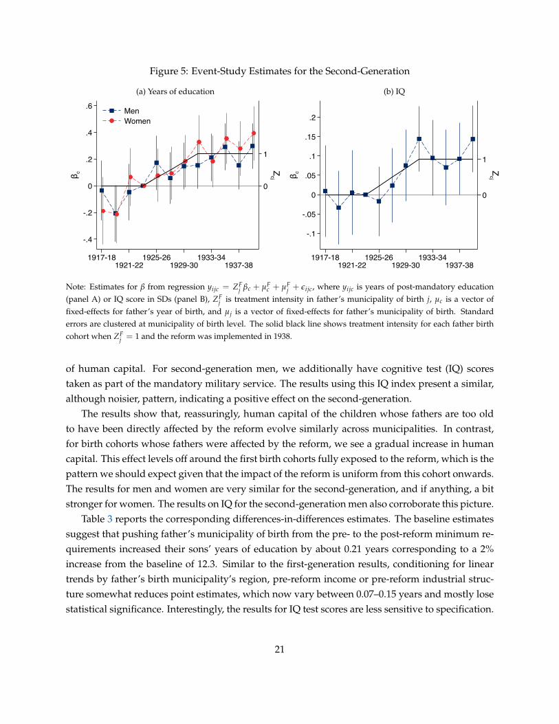
Figure 5: Event-Study Estimates for the Second-Generation

(a) Years of education

0

1

Zcj

-.4

-.2

0

.2

.4

.6

β c

1917-181921-22

1925-261929-30

1933-341937-38

MenWomen

(b) IQ

0

1

Zcj

-.1

-.05

0

.05

.1

.15

.2

β c

1917-181921-22

1925-261929-30

1933-341937-38

Note: Estimates for β from regression yijc = ZFj βc + µF

c + µFj + εijc, where yijc is years of post-mandatory education

(panel A) or IQ score in SDs (panel B), ZFj is treatment intensity in father’s municipality of birth j, µc is a vector of

fixed-effects for father’s year of birth, and µj is a vector of fixed-effects for father’s municipality of birth. Standarderrors are clustered at municipality of birth level. The solid black line shows treatment intensity for each father birthcohort when ZF

j = 1 and the reform was implemented in 1938.

of human capital. For second-generation men, we additionally have cognitive test (IQ) scorestaken as part of the mandatory military service. The results using this IQ index present a similar,although noisier, pattern, indicating a positive effect on the second-generation.

The results show that, reassuringly, human capital of the children whose fathers are too oldto have been directly affected by the reform evolve similarly across municipalities. In contrast,for birth cohorts whose fathers were affected by the reform, we see a gradual increase in humancapital. This effect levels off around the first birth cohorts fully exposed to the reform, which is thepattern we should expect given that the impact of the reform is uniform from this cohort onwards.The results for men and women are very similar for the second-generation, and if anything, a bitstronger for women. The results on IQ for the second-generation men also corroborate this picture.

Table 3 reports the corresponding differences-in-differences estimates. The baseline estimatessuggest that pushing father’s municipality of birth from the pre- to the post-reform minimum re-quirements increased their sons’ years of education by about 0.21 years corresponding to a 2%increase from the baseline of 12.3. Similar to the first-generation results, conditioning for lineartrends by father’s birth municipality’s region, pre-reform income or pre-reform industrial struc-ture somewhat reduces point estimates, which now vary between 0.07–0.15 years and mostly losestatistical significance. Interestingly, the results for IQ test scores are less sensitive to specification.

21

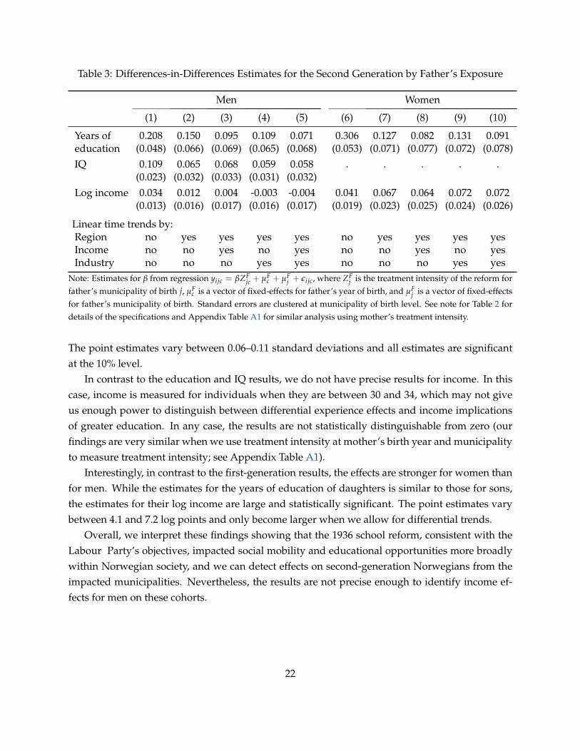
Table 3: Differences-in-Differences Estimates for the Second Generation by Father’s Exposure

Men Women

(1) (2) (3) (4) (5) (6) (7) (8) (9) (10)

Years of 0.208 0.150 0.095 0.109 0.071 0.306 0.127 0.082 0.131 0.091education (0.048) (0.066) (0.069) (0.065) (0.068) (0.053) (0.071) (0.077) (0.072) (0.078)IQ 0.109 0.065 0.068 0.059 0.058 . . . . .

(0.023) (0.032) (0.033) (0.031) (0.032)Log income 0.034 0.012 0.004 -0.003 -0.004 0.041 0.067 0.064 0.072 0.072

(0.013) (0.016) (0.017) (0.016) (0.017) (0.019) (0.023) (0.025) (0.024) (0.026)

Linear time trends by:Region no yes yes yes yes no yes yes yes yesIncome no no yes no yes no no yes no yesIndustry no no no yes yes no no no yes yes

Note: Estimates for β from regression yijc = βZFjc + µF

c + µFj + εijc, where ZF

j is the treatment intensity of the reform forfather’s municipality of birth j, µF

c is a vector of fixed-effects for father’s year of birth, and µFj is a vector of fixed-effects

for father’s municipality of birth. Standard errors are clustered at municipality of birth level. See note for Table 2 fordetails of the specifications and Appendix Table A1 for similar analysis using mother’s treatment intensity.

The point estimates vary between 0.06–0.11 standard deviations and all estimates are significantat the 10% level.

In contrast to the education and IQ results, we do not have precise results for income. In thiscase, income is measured for individuals when they are between 30 and 34, which may not giveus enough power to distinguish between differential experience effects and income implicationsof greater education. In any case, the results are not statistically distinguishable from zero (ourfindings are very similar when we use treatment intensity at mother’s birth year and municipalityto measure treatment intensity; see Appendix Table A1).

Interestingly, in contrast to the first-generation results, the effects are stronger for women thanfor men. While the estimates for the years of education of daughters is similar to those for sons,the estimates for their log income are large and statistically significant. The point estimates varybetween 4.1 and 7.2 log points and only become larger when we allow for differential trends.

Overall, we interpret these findings showing that the 1936 school reform, consistent with theLabour Party’s objectives, impacted social mobility and educational opportunities more broadlywithin Norwegian society, and we can detect effects on second-generation Norwegians from theimpacted municipalities. Nevertheless, the results are not precise enough to identify income ef-fects for men on these cohorts.

22

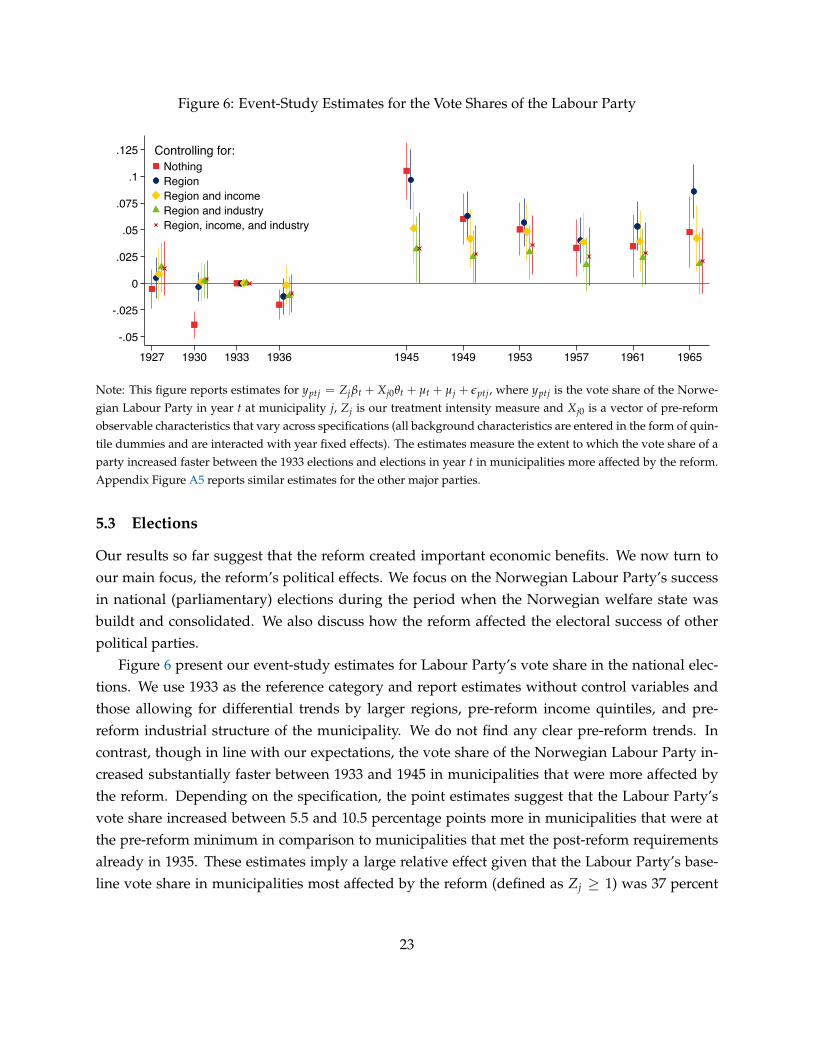
Figure 6: Event-Study Estimates for the Vote Shares of the Labour Party

-.05

-.025

0

.025

.05

.075

.1

.125

1927 1930 1933 1936 1945 1949 1953 1957 1961 1965

NothingRegionRegion and incomeRegion and industryRegion, income, and industry

Controlling for:

Note: This figure reports estimates for yptj = Zjβt + Xj0θt + µt + µj + εptj, where yptj is the vote share of the Norwe-gian Labour Party in year t at municipality j, Zj is our treatment intensity measure and Xj0 is a vector of pre-reformobservable characteristics that vary across specifications (all background characteristics are entered in the form of quin-tile dummies and are interacted with year fixed effects). The estimates measure the extent to which the vote share of aparty increased faster between the 1933 elections and elections in year t in municipalities more affected by the reform.Appendix Figure A5 reports similar estimates for the other major parties.

5.3 Elections

Our results so far suggest that the reform created important economic benefits. We now turn toour main focus, the reform’s political effects. We focus on the Norwegian Labour Party’s successin national (parliamentary) elections during the period when the Norwegian welfare state wasbuildt and consolidated. We also discuss how the reform affected the electoral success of otherpolitical parties.

Figure 6 present our event-study estimates for Labour Party’s vote share in the national elec-tions. We use 1933 as the reference category and report estimates without control variables andthose allowing for differential trends by larger regions, pre-reform income quintiles, and pre-reform industrial structure of the municipality. We do not find any clear pre-reform trends. Incontrast, though in line with our expectations, the vote share of the Norwegian Labour Party in-creased substantially faster between 1933 and 1945 in municipalities that were more affected bythe reform. Depending on the specification, the point estimates suggest that the Labour Party’svote share increased between 5.5 and 10.5 percentage points more in municipalities that were atthe pre-reform minimum in comparison to municipalities that met the post-reform requirementsalready in 1935. These estimates imply a large relative effect given that the Labour Party’s base-line vote share in municipalities most affected by the reform (defined as Zj ≥ 1) was 37 percent

23

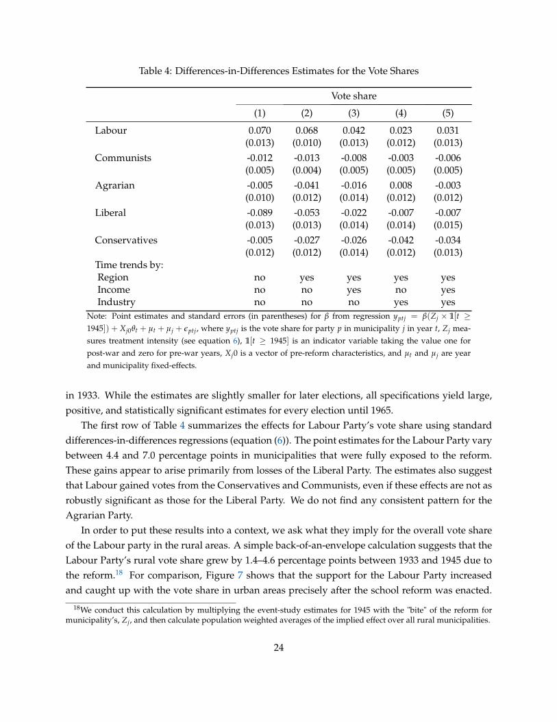
Table 4: Differences-in-Differences Estimates for the Vote Shares

Vote share

(1) (2) (3) (4) (5)

Labour 0.070 0.068 0.042 0.023 0.031(0.013) (0.010) (0.013) (0.012) (0.013)

Communists -0.012 -0.013 -0.008 -0.003 -0.006(0.005) (0.004) (0.005) (0.005) (0.005)

Agrarian -0.005 -0.041 -0.016 0.008 -0.003(0.010) (0.012) (0.014) (0.012) (0.012)

Liberal -0.089 -0.053 -0.022 -0.007 -0.007(0.013) (0.013) (0.014) (0.014) (0.015)

Conservatives -0.005 -0.027 -0.026 -0.042 -0.034(0.012) (0.012) (0.014) (0.012) (0.013)

Time trends by:Region no yes yes yes yesIncome no no yes no yesIndustry no no no yes yes

Note: Point estimates and standard errors (in parentheses) for β from regression yptj = β(Zj × 1[t ≥1945]) + Xj0θt + µt + µj + εptj, where yptj is the vote share for party p in municipality j in year t, Zj mea-sures treatment intensity (see equation 6), 1[t ≥ 1945] is an indicator variable taking the value one forpost-war and zero for pre-war years, Xj0 is a vector of pre-reform characteristics, and µt and µj are yearand municipality fixed-effects.

in 1933. While the estimates are slightly smaller for later elections, all specifications yield large,positive, and statistically significant estimates for every election until 1965.

The first row of Table 4 summarizes the effects for Labour Party’s vote share using standarddifferences-in-differences regressions (equation (6)). The point estimates for the Labour Party varybetween 4.4 and 7.0 percentage points in municipalities that were fully exposed to the reform.These gains appear to arise primarily from losses of the Liberal Party. The estimates also suggestthat Labour gained votes from the Conservatives and Communists, even if these effects are not asrobustly significant as those for the Liberal Party. We do not find any consistent pattern for theAgrarian Party.

In order to put these results into a context, we ask what they imply for the overall vote shareof the Labour party in the rural areas. A simple back-of-an-envelope calculation suggests that theLabour Party’s rural vote share grew by 1.4–4.6 percentage points between 1933 and 1945 due tothe reform.18 For comparison, Figure 7 shows that the support for the Labour Party increasedand caught up with the vote share in urban areas precisely after the school reform was enacted.

18We conduct this calculation by multiplying the event-study estimates for 1945 with the "bite" of the reform formunicipality’s, Zj, and then calculate population weighted averages of the implied effect over all rural municipalities.

24

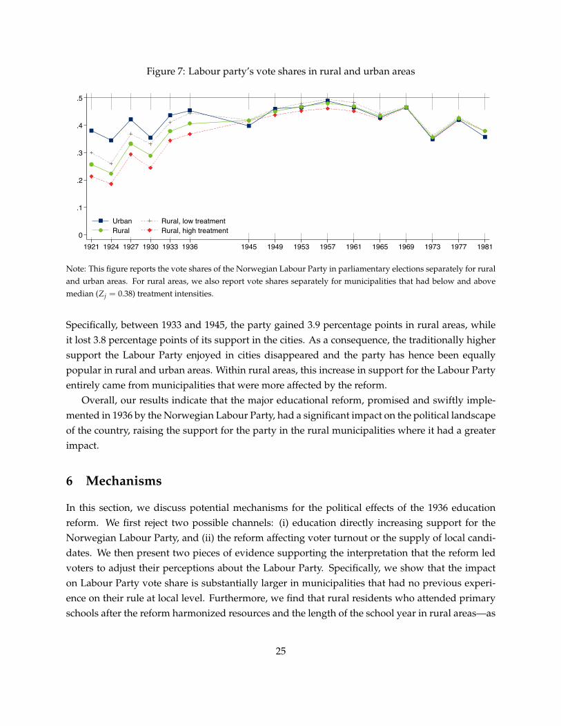
Figure 7: Labour party’s vote shares in rural and urban areas

0

.1

.2

.3

.4

.5

1921 1924 1927 1930 1933 1936 1945 1949 1953 1957 1961 1965 1969 1973 1977 1981

Urban Rural, low treatmentRural Rural, high treatment

Note: This figure reports the vote shares of the Norwegian Labour Party in parliamentary elections separately for ruraland urban areas. For rural areas, we also report vote shares separately for municipalities that had below and abovemedian (Zj = 0.38) treatment intensities.

Specifically, between 1933 and 1945, the party gained 3.9 percentage points in rural areas, whileit lost 3.8 percentage points of its support in the cities. As a consequence, the traditionally highersupport the Labour Party enjoyed in cities disappeared and the party has hence been equallypopular in rural and urban areas. Within rural areas, this increase in support for the Labour Partyentirely came from municipalities that were more affected by the reform.

Overall, our results indicate that the major educational reform, promised and swiftly imple-mented in 1936 by the Norwegian Labour Party, had a significant impact on the political landscapeof the country, raising the support for the party in the rural municipalities where it had a greaterimpact.

6 Mechanisms

In this section, we discuss potential mechanisms for the political effects of the 1936 educationreform. We first reject two possible channels: (i) education directly increasing support for theNorwegian Labour Party, and (ii) the reform affecting voter turnout or the supply of local candi-dates. We then present two pieces of evidence supporting the interpretation that the reform ledvoters to adjust their perceptions about the Labour Party. Specifically, we show that the impacton Labour Party vote share is substantially larger in municipalities that had no previous experi-ence on their rule at local level. Furthermore, we find that rural residents who attended primaryschools after the reform harmonized resources and the length of the school year in rural areas—as

25

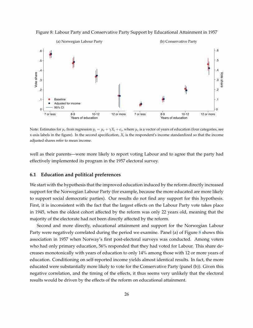
Figure 8: Labour Party and Conservative Party Support by Educational Attainment in 1957

(a) Norwegian Labour Party

0

.1

.2

.3

.4

.5

.6

Vote

sha

re

7 or less 8-9 10-12 12 or moreYears of education

BaselineAdjusted for income95% CI

(b) Conservative Party

0

.1

.2

.3

.4

.5

.6

Vote share

7 or less 8-9 10-12 12 or moreYears of education

Note: Estimates for µe from regression yi = µe +γXi + εi, where µe is a vector of years of education (four categories, seex-axis labels in the figure). In the second specification, Xi is the respondent’s income standardized so that the incomeadjusted shares refer to mean income.

well as their parents—were more likely to report voting Labour and to agree that the party hadeffectively implemented its program in the 1957 electoral survey.

6.1 Education and political preferences

We start with the hypothesis that the improved education induced by the reform directly increasedsupport for the Norwegian Labour Party (for example, because the more educated are more likelyto support social democratic parties). Our results do not find any support for this hypothesis.First, it is inconsistent with the fact that the largest effects on the Labour Party vote takes placein 1945, when the oldest cohort affected by the reform was only 22 years old, meaning that themajority of the electorate had not been directly affected by the reform.

Second and more directly, educational attainment and support for the Norwegian LabourParty were negatively correlated during the period we examine. Panel (a) of Figure 8 shows thisassociation in 1957 when Norway’s first post-electoral surveys was conducted. Among voterswho had only primary education, 56% responded that they had voted for Labour. This share de-creases monotonically with years of education to only 14% among those with 12 or more years ofeducation. Conditioning on self-reported income yields almost identical results. In fact, the moreeducated were substantially more likely to vote for the Conservative Party (panel (b)). Given thisnegative correlation, and the timing of the effects, it thus seems very unlikely that the electoralresults would be driven by the effects of the reform on educational attainment.

26

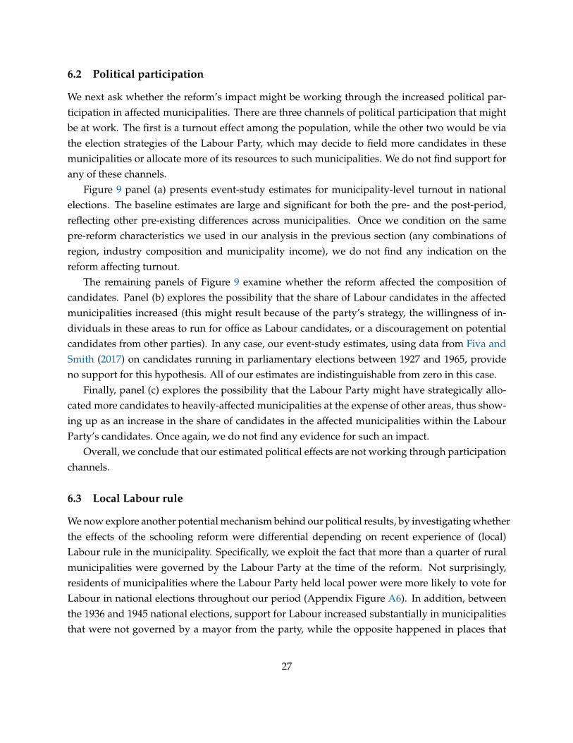
6.2 Political participation

We next ask whether the reform’s impact might be working through the increased political par-ticipation in affected municipalities. There are three channels of political participation that mightbe at work. The first is a turnout effect among the population, while the other two would be viathe election strategies of the Labour Party, which may decide to field more candidates in thesemunicipalities or allocate more of its resources to such municipalities. We do not find support forany of these channels.

Figure 9 panel (a) presents event-study estimates for municipality-level turnout in nationalelections. The baseline estimates are large and significant for both the pre- and the post-period,reflecting other pre-existing differences across municipalities. Once we condition on the samepre-reform characteristics we used in our analysis in the previous section (any combinations ofregion, industry composition and municipality income), we do not find any indication on thereform affecting turnout.

The remaining panels of Figure 9 examine whether the reform affected the composition ofcandidates. Panel (b) explores the possibility that the share of Labour candidates in the affectedmunicipalities increased (this might result because of the party’s strategy, the willingness of in-dividuals in these areas to run for office as Labour candidates, or a discouragement on potentialcandidates from other parties). In any case, our event-study estimates, using data from Fiva andSmith (2017) on candidates running in parliamentary elections between 1927 and 1965, provideno support for this hypothesis. All of our estimates are indistinguishable from zero in this case.

Finally, panel (c) explores the possibility that the Labour Party might have strategically allo-cated more candidates to heavily-affected municipalities at the expense of other areas, thus show-ing up as an increase in the share of candidates in the affected municipalities within the LabourParty’s candidates. Once again, we do not find any evidence for such an impact.

Overall, we conclude that our estimated political effects are not working through participationchannels.

6.3 Local Labour rule

We now explore another potential mechanism behind our political results, by investigating whetherthe effects of the schooling reform were differential depending on recent experience of (local)Labour rule in the municipality. Specifically, we exploit the fact that more than a quarter of ruralmunicipalities were governed by the Labour Party at the time of the reform. Not surprisingly,residents of municipalities where the Labour Party held local power were more likely to vote forLabour in national elections throughout our period (Appendix Figure A6). In addition, betweenthe 1936 and 1945 national elections, support for Labour increased substantially in municipalitiesthat were not governed by a mayor from the party, while the opposite happened in places that

27

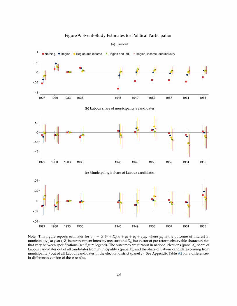
Figure 9: Event-Study Estimates for Political Participation

(a) Turnout

-.1

-.05

0

.05

.1

1927 1930 1933 1936 1945 1949 1953 1957 1961 1965

Nothing Region Region and income Region and ind. Region, income, and industry

(b) Labour share of municipality’s candidates

-.3

-.15

0

.15

1927 1930 1933 1936 1945 1949 1953 1957 1961 1965

(c) Municipality’s share of Labour candidates

-.04

-.02

0

.02

.04

1927 1930 1933 1936 1945 1949 1953 1957 1961 1965

Note: This figure reports estimates for ytj = Zjβt + Xj0θt + µt + µj + εptj, where ytj is the outcome of interest inmunicipality j at year t, Zj is our treatment intensity measure and Xj0 is a vector of pre-reform observable characteristicsthat vary between specifications (see figure legend). The outcomes are turnout in national elections (panel a), share ofLabour candidates out of all candidates from municipality j (panel b), and the share of Labour candidates coming frommunicipality j out of all Labour candidates in the election district (panel c). See Appendix Table A2 for a differences-in-differences version of these results.

28

Figure 10: Labor Vote Share Estimates by Earlier Exposure to Local Labour Rule

(a) Non-Labour Mayor in 1934

-.08

-.04

0

.04

.08

.12

19271930

19331936

19451949

19531957

19611965

NothingRegionRegion and incomeRegion and industryRegion, income,and industry

Controlling for:

(b) Labour Mayor in 1934

-.08

-.04

0

.04

.08

.12

19271930

19331936

19451949

19531957

19611965

Note: This figure reports results from regression yptj = Zjβt + Wjγt + (Zj × Wj)δt + Xj0θt + µt + µj + εptj, where yptj

is the vote share of the Norwegian Labour Party in year t at municipality j, Zj treatment intensity, Wj is an indicatorfor the municipality having a Labour mayor in 1934, Xj0 is a vector of pre-reform observable characteristics that varybetween specifications (see figure legend), and µt and µj are year and municipality fixed-effects, respectively. Panel (a)reports estimates for βt, i.e., the impact of the reform on municipalities with no prior exposure to Labour rule. Panel (b)reports estimates for βt + δt, i.e., effects for other municipalities that had a Labour mayor in 1934. See Appendix TableA3 for a differences-in-differences version of these results.

were already under local Labor rule at the time the party assumed national power.19

The event-study estimates reported in Figure 10 show that the effects of the 1936 school reformare significantly larger in non-Labour municipalities. We construct the figure by first estimating

yptj = Zjβt + Wjγt + (Zj × Wj)δt + Xj0θt + µt + µj + εptj (7)

where yptj is the vote share of the Labour party in the national elections in year t at municipality j,Wj is an indicator variable taking value one if the local mayor in 1934 was from the Labour Partyand zero otherwise, and Zj and Xj0 are the same pre-reform distance and pre-reform observablecharacteristics as in our baseline analysis. Panel (a) of Figure 10 reports estimates for β̂, whichcaptures the effect of the schooling reform on municipalities that did not have Labour local gov-ernment. Similarly, panel (b) of Figure 10 reports estimates for β̂ + δ̂, corresponding to the effectof schooling reform on municipalities that had a Labour mayor in 1934.

19We define local Labour rule using data on the political affiliation of the mayor after the 1934 local elections. Whilesome geographical clustering is evident (Appendix Figure A6), there are municipalities under Labour control in allparts of the country. Municipalities in both groups are also present over the entire support of the treatment intensitydistribution (Appendix Figure A7).

29

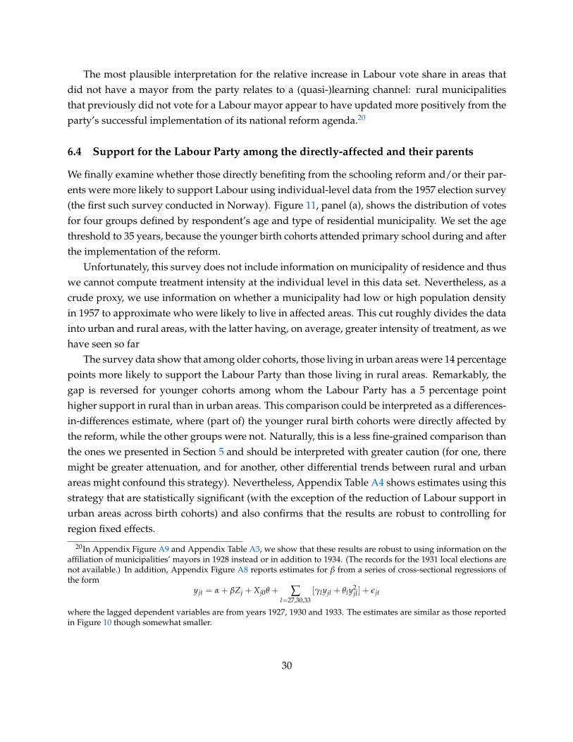
The most plausible interpretation for the relative increase in Labour vote share in areas thatdid not have a mayor from the party relates to a (quasi-)learning channel: rural municipalitiesthat previously did not vote for a Labour mayor appear to have updated more positively from theparty’s successful implementation of its national reform agenda.20

6.4 Support for the Labour Party among the directly-affected and their parents

We finally examine whether those directly benefiting from the schooling reform and/or their par-ents were more likely to support Labour using individual-level data from the 1957 election survey(the first such survey conducted in Norway). Figure 11, panel (a), shows the distribution of votesfor four groups defined by respondent’s age and type of residential municipality. We set the agethreshold to 35 years, because the younger birth cohorts attended primary school during and afterthe implementation of the reform.

Unfortunately, this survey does not include information on municipality of residence and thuswe cannot compute treatment intensity at the individual level in this data set. Nevertheless, as acrude proxy, we use information on whether a municipality had low or high population densityin 1957 to approximate who were likely to live in affected areas. This cut roughly divides the datainto urban and rural areas, with the latter having, on average, greater intensity of treatment, as wehave seen so far

The survey data show that among older cohorts, those living in urban areas were 14 percentagepoints more likely to support the Labour Party than those living in rural areas. Remarkably, thegap is reversed for younger cohorts among whom the Labour Party has a 5 percentage pointhigher support in rural than in urban areas. This comparison could be interpreted as a differences-in-differences estimate, where (part of) the younger rural birth cohorts were directly affected bythe reform, while the other groups were not. Naturally, this is a less fine-grained comparison thanthe ones we presented in Section 5 and should be interpreted with greater caution (for one, theremight be greater attenuation, and for another, other differential trends between rural and urbanareas might confound this strategy). Nevertheless, Appendix Table A4 shows estimates using thisstrategy that are statistically significant (with the exception of the reduction of Labour support inurban areas across birth cohorts) and also confirms that the results are robust to controlling forregion fixed effects.

20In Appendix Figure A9 and Appendix Table A3, we show that these results are robust to using information on theaffiliation of municipalities’ mayors in 1928 instead or in addition to 1934. (The records for the 1931 local elections arenot available.) In addition, Appendix Figure A8 reports estimates for β from a series of cross-sectional regressions ofthe form

yjt = α + βZj + Xj0θ + ∑l=27,30,33

[γlyjl + θly2jl ] + εjt

where the lagged dependent variables are from years 1927, 1930 and 1933. The estimates are similar as those reportedin Figure 10 though somewhat smaller.

30

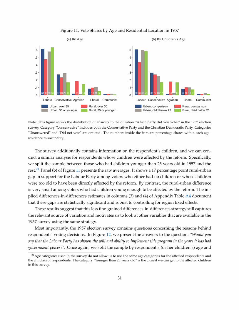
Figure 11: Vote Shares by Age and Residential Location in 1957

(a) By Age

61 27 848 23 18 1058 29 1163 17 14 50

.1

.2

.3

.4

.5

.6

Labour Conservative Agrarian Liberal Communist

Urban, over 35 Rural, over 35Urban, 35 or younger Rural, 35 or younger

(b) By Children’s Age

30 860 2743 18 10 102660 758 17170

.1

.2

.3

.4

.5

.6

Labour Conservative Agrarian Liberal Communist

Urban, comparison Rural, comparisonUrban, child below 25 Rural, child below 25

Note: This figure shows the distribution of answers to the question "Which party did you vote?" in the 1957 electionsurvey. Category "Conservative" includes both the Conservative Party and the Christian Democratic Party. Categories"Unanswered" and "Did not vote" are omitted. The numbers inside the bars are percentage shares within each age–residence municipality.

The survey additionally contains information on the respondent’s children, and we can con-duct a similar analysis for respondents whose children were affected by the reform. Specifically,we split the sample between those who had children younger than 25 years old in 1957 and therest.21 Panel (b) of Figure 11 presents the raw averages. It shows a 17 percentage point rural-urbangap in support for the Labour Party among voters who either had no children or whose childrenwere too old to have been directly affected by the reform. By contrast, the rural-urban differenceis very small among voters who had children young enough to be affected by the reform. The im-plied differences-in-differences estimates in columns (3) and (4) of Appendix Table A4 documentthat these gaps are statistically significant and robust to controlling for region fixed effects.

These results suggest that this less fine-grained differences-in-differences strategy still capturesthe relevant source of variation and motivates us to look at other variables that are available in the1957 survey using the same strategy.

Most importantly, the 1957 election survey contains questions concerning the reasons behindrespondents’ voting decisions. In Figure 12, we present the answers to the question: "Would yousay that the Labour Party has shown the will and ability to implement this program in the years it has hadgovernment power?". Once again, we split the sample by respondent’s (or her children’s) age and

21Age categories used in the survey do not allow us to use the same age categories for the affected respondents andthe children of respondents. The category "Younger than 25 years old" is the closest we can get to the affected childrenin this survey.

31

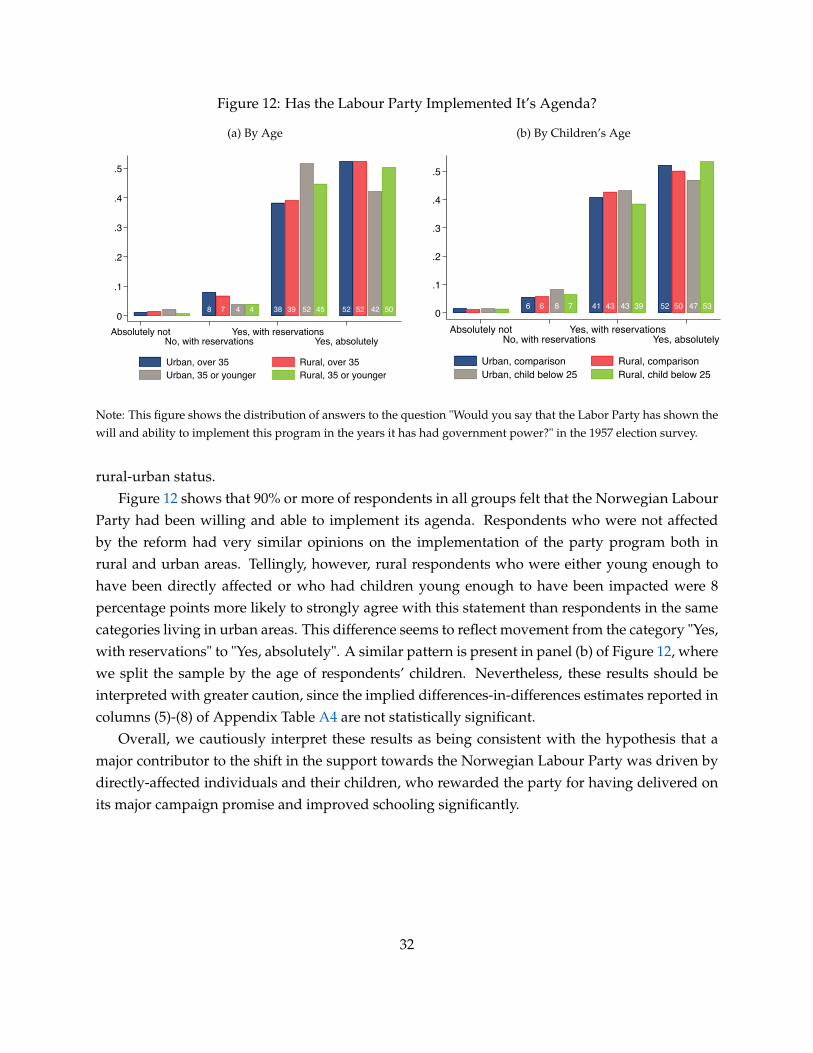
Figure 12: Has the Labour Party Implemented It’s Agenda?

(a) By Age

8 38 521 52397 524 42 50451 40

.1

.2

.3

.4

.5

Absolutely notNo, with reservations

Yes, with reservationsYes, absolutely

Urban, over 35 Rural, over 35Urban, 35 or younger Rural, 35 or younger

(b) By Children’s Age

416 5243 506 47438 397 530

.1

.2

.3

.4

.5

Absolutely notNo, with reservations

Yes, with reservationsYes, absolutely

Urban, comparison Rural, comparisonUrban, child below 25 Rural, child below 25

Note: This figure shows the distribution of answers to the question "Would you say that the Labor Party has shown thewill and ability to implement this program in the years it has had government power?" in the 1957 election survey.

rural-urban status.Figure 12 shows that 90% or more of respondents in all groups felt that the Norwegian Labour

Party had been willing and able to implement its agenda. Respondents who were not affectedby the reform had very similar opinions on the implementation of the party program both inrural and urban areas. Tellingly, however, rural respondents who were either young enough tohave been directly affected or who had children young enough to have been impacted were 8percentage points more likely to strongly agree with this statement than respondents in the samecategories living in urban areas. This difference seems to reflect movement from the category "Yes,with reservations" to "Yes, absolutely". A similar pattern is present in panel (b) of Figure 12, wherewe split the sample by the age of respondents’ children. Nevertheless, these results should beinterpreted with greater caution, since the implied differences-in-differences estimates reported incolumns (5)-(8) of Appendix Table A4 are not statistically significant.

Overall, we cautiously interpret these results as being consistent with the hypothesis that amajor contributor to the shift in the support towards the Norwegian Labour Party was driven bydirectly-affected individuals and their children, who rewarded the party for having delivered onits major campaign promise and improved schooling significantly.

32

7 Conclusions

The 19th and early 20th centuries witnessed major challenges to the then-prevailing “capitalist sys-tems”. While some of these challenges were strongly influenced by Marxist/socialist ideas andattempted to overthrow the existing system, others took a decidedly reformist approach, workingthrough democratic process and seeking power in order to implement fundamental reform withinthe broader institutional structure of their countries. This reformist approach is most closely iden-tified with the social democratic parties in Scandinavia, which were initially influenced by thesame socialist ideas but then broke away from the Marxist tradition. Starting with Sweden in1932, social democratic (labor or worker) parties in these countries came to power and imple-mented sweeping reforms. The key social democratic policy and institutional reforms includedthe strengthening of trade unions; the development of a corporatist model of wage setting withnegotiations between trade unions, employers and the government; active macroeconomic man-agement; progressive taxation; national health care systems; social security; various other socialprograms; and also centrally, greater investment in publicly-provided education.

The Norwegian Labour Party, which assumed power in 1935, provides an ideal case studyfor understanding how the social democratic system came to be formed, in part because it cam-paigned with the promise to undertake a major schooling reform. As soon as it was in power, itimplemented its promised reform, which harmonized the school year, raising minimum instruc-tion time in economically less developed rural areas and boosting the resources available to ruralschools.

We document that cohorts that were more intensively treated by this school reform—becauseof their location and age at the time of reform—significantly increased their education. There isalso evidence that their subsequent labor income rose as well, though these estimates are some-times less precise because of other confounding trends favoring rural areas.

More importantly, we find that residents of municipalities that benefited from the 1936 school-ing reform became much more likely to vote for the Labour Party. Perhaps even more strikingly,the additional support for this party persisted for several decades.

Our evidence suggests that these results are not mediated by the direct effects of education(in fact, more educated individuals were less likely to support the Labour Party at the time). Norare they explained by greater participation or greater attention from the Labour Party towardsthese municipalities. Rather, our evidence suggests that cohorts that benefited from the schoolingreform, as well as their parents, rewarded the party for having kept its promise and for deliveringa major reform.

Several economists and commentators are presently calling for major institutional reforms inWestern nations (e.g. Esping-Andersen et al. 2002; Rajan 2019; Stiglitz 2019). A key question iswhether the Norwegian experience in the 1930s is relevant for the current context and whether a

33

credible promise and later delivery of major reforms could be the basis of a broad coalition thatsupports these reforms and the parties that implement them. While we have no direct answer tothis question, we believe that a systematic analysis of the interplay between economic and socialreforms and the formation of different political coalitions is an interesting area for future research.

References

Aaberge, R., A. B. Atkinson, and J. Modalsli (2020). Estimating long-run income inequality frommixed tabular data: Empirical evidence from Norway, 1875–2017. Journal of Public Economics 187,104196.

Acemoglu, D., N. Ajzenman, C. Giray Aksoy, M. Fiszbein, and C. Molina (2021). (Successful)Democracies Breed Their Own Support. Working paper.

Acemoglu, D. and J. Angrist (2000). How large are human-capital externalities? Evidence fromcompulsory schooling laws. NBER Macroeconomics Annual 15, 9–59.

Acemoglu, D., G. Egorov, and K. Sonin (2013). A Political Theory of Populism. Quarterly Journalof Economics 128(2), 771–805.

Acemoglu, D. and S. Johnson (2007). Disease and Development: The Effect of Life Expectancy onEconomic Growth. Journal of Political Economy 115(6), 925–985.

Acemoglu, D., S. Johnson, J. A. Robinson, and P. Yared (2005). From education to democracy?American Economic Review 95(2), 44–49.

Acemoglu, D., S. Johnson, J. A. Robinson, and P. Yared (2008). Income and democracy. AmericanEconomic Review 98(3), 808–42.

Acemoglu, D. and J. A. Robinson (2006). Economic Origins of Dictatorship and Democracy. Cam-bridge University Press.

Acemoglu, D. and J. A. Robinson (2012). Why Nations Fail: The Origins of Power, Prosperity, andPoverty. Currency.

Atkinson, A. B. and J. E. Søgaard (2016). The long-run history of income inequality in Denmark.The Scandinavian Journal of Economics 118(2), 264–291.

Baldwin, P. (1990). The Politics of Social Solidarity: Class Bases of the European Welfare State, 1875-1975.Cambridge University Press.

Bengtsson, E. (2019). The Swedish Sonderweg in question: Democratization and inequality incomparative perspective, c. 1750–1920. Past & Present 244(1), 123–161.

34

Berman, S. (2006). The primacy of politics: Social democracy and the making of Europe’s twentieth century.Cambridge University Press.

Bidner, C. and P. François (2013). The emergence of political accountability. The Quarterly Journalof Economics 128(3), 1397–1448.

Björklund, A., M. Jäntti, and M. J. Lindquist (2009). Family background and income during therise of the welfare state: brother correlations in income for swedish men born 1932–1968. Journalof Public Economics 93(5-6), 671–680.

Bjørnson, Ø. (2001). The social democrats and the norwegian welfare state: some perspectives.Scandinavian Journal of History 26(3), 197–223.

Black, S. E., P. J. Devereux, and K. G. Salvanes (2005). Why the apple doesn’t fall far: Understand-ing intergenerational transmission of human capital. American Economic Review 95(1), 437–449.

Brender, A. and A. Drazen (2007). Electoral fiscal policy in new, old, and fragile democracies.Comparative Economic Studies 49(3), 446–466.

Bull, E. (1959). Kriseforliket mellom bondepartiet og det norske arbeiderparti i 1935. Historisktidsskrift 39, 126.

Caprettini, B., L. Casaburi, and M. Venturini (2021). The Electoral Impact of Wealth Redistribution:Evidence from the Italian Land Reform. Working paper.

Card, D. (1992). Using Regional Variation in Wages to Measure the Effects of the Federal MinimumWage. ILR Review 46(1), 22–37.

Cox, G. W., J. H. Fiva, and D. M. Smith (2019). Parties, legislators, and the origins of proportionalrepresentation. Comparative Political Studies 52(1), 102–133.

Dahl, H. F. (1971). Norge mellom krigene: Det norske samfunn i krise og konflikt 1918-1940. Pax.

Duflo, E. (2001). Schooling and labor market consequences of school construction in Indonesia:Evidence from an unusual policy experiment. American Economic Review 91(4), 795–813.

Esping-Andersen, G. (1985). Power and distributional regimes. Politics & Society 14(2), 223–256.

Esping-Andersen, G. (1990). The three worlds of welfare capitalism. Princeton University Press.

Esping-Andersen, G., D. Gallie, A. Hemerijck, and J. Myles (2002). Why We Need a New WelfareState. Oxford University Press.

Falk, T. and P. Tovmo (2000). Norwegian local public finance in the 1930s. Unpublished paper,Norwegian University of Science and Technology. Trondheim, Norway.

35

Fearon, J. D. (2011). Self-enforcing democracy. The Quarterly Journal of Economics 126(4), 1661–1708.

Ferejohn, J. (1986). Incumbent performance and electoral control. Public choice 50(1), 5–25.

Fernandez, R. and D. Rodrik (1991). Resistance to reform: Status quo bias in the presence ofindividual-specific uncertainty. American Economic Review, 1146–1155.

Finan, F. and L. Schechter (2012). Vote-buying and reciprocity. Econometrica 80(2), 863–881.

Fiva, J. H. and D. M. Smith (2017). Norwegian parliamentary elections, 1906–2013: representationand turnout across four electoral systems. West European Politics 40(6), 1373–1391.

Friedman, W., M. Kremer, E. Miguel, and R. Thornton (2016). Education as liberation? Econom-ica 83(329), 1–30.

Giavazzi, F. and G. Tabellini (2005). Economic and political liberalizations. Journal of MonetaryEconomics 52(7), 1297–1330.

Glaeser, E. L., G. A. Ponzetto, and A. Shleifer (2007). Why does democracy need education? Journalof Economic Growth 12(2), 77–99.

Gourevitch, P. (1986). Politics in hard times: Comparative responses to international economic crises.Cornell University Press.

Grossman, G. M. and E. Helpman (2001). Special interest politics. MIT press.

Korpi, W. (1983). The Democratic Class Struggle. Routledge.

Lewin, L. (1967). Planhushållningsdebatten. Ph. D. thesis, Acta Universitatis Upsaliensis.

Lipset, S. M. (1959). Some social requisites of democracy: Economic development and politicallegitimacy. American Political Science Review 53(1), 69–105.

Mediås, O. A. (2004). Enhetsskolens utvikling i Danmark og Norge: allmueskolen, folkeskolen,grunnskolen i utvikling fra de første skolelover og fram til år 2003. Aalborg Universitetsforlag.

Meghir, C. and M. Palme (2005). Educational reform, ability, and family background. AmericanEconomic Review 95(1), 414–424.

Meriläinen, J., M. Mitrunen, and T. Virkola (2020). The Violent Origins of Finnish Equality. Work-ing paper.

Milligan, K., E. Moretti, and P. Oreopoulos (2004). Does education improve citizenship? Evidencefrom the United States and the United Kingdom. Journal of Public Economics 88(9-10), 1667–1695.

36

Moene, K. O. and M. Wallerstein (2006). Social democracy as a development strategy. Globalizationand egalitarian redistribution, 148–168.

Oreopoulos, P. (2006). Estimating average and local average treatment effects of education whencompulsory schooling laws really matter. American Economic Review 96(1), 152–175.

Oreopoulos, P. and K. G. Salvanes (2011). Priceless: The nonpecuniary benefits of schooling. Jour-nal of Economic perspectives 25(1), 159–84.

Pekkarinen, T., K. G. Salvanes, and M. Sarvimäki (2017). The evolution of social mobility: Norwayduring the twentieth century. The Scandinavian Journal of Economics 119(1), 5–33.

Pekkarinen, T., R. Uusitalo, and S. Kerr (2009). School tracking and intergenerational income mo-bility: Evidence from the finnish comprehensive school reform. Journal of Public Economics 93(7-8), 965–973.

Persson, T., G. Tabellini, et al. (2000). Political Economics: Explaining Economic Policy. MIT pressCambridge, MA.

Rajan, R. (2019). The Third Pillar: How Markets and the State Leave the Community Behind. Penguin.

Rokkan, S., U. Torgersen, H. Valen, and G. Dupeux (1958). Les élections norvégiennes du 7 octobre1957. Revue française de science politique 8(1), 73–94.

Rothstein, B. (1998). The Social Democratic State: Swedish Model And The Bureaucratic Problem. Uni-versity of Pittsburgh Pre.

Rust, V. D. (1989). The democratic tradition and the evolution of schooling in Norway, Volume 34.Praeger.

Sejersted, F. (2011). The age of social democracy: Norway and Sweden in the twentieth century. PrincetonUniversity Press.

Stiglitz, J. (2019). People, power, and profits: Progressive capitalism for an age of discontent. PenguinUK.

Strulovici, B. (2010). Learning while voting: Determinants of collective experimentation. Econo-metrica 78(3), 933–971.

Sundet, J. M., D. G. Barlaug, and T. M. Torjussen (2004). The end of the Flynn effect?: A study ofsecular trends in mean intelligence test scores of Norwegian conscripts during half a century.Intelligence 32(4), 349–362.

Verba, S. and G. Almond (1963). The Civic Culture: Political attitudes and democracy in five nations.Princeton, NJ: Princeton University Press.

37

Appendix tables and figures

Figure A1: Norwegian Labour Party’s Election Posters

(a) 1930 (b) 1933

Note: The change in the rhetoric of the Norwegian Labour Party as illustrated by election posters. Both are designedby the same artist, Erling Nielsen. The 1930 campaign focused on urban industrial workers and the poster design isheavily influenced by Soviet art. The 1933 campaign led with a message of unity and the poster includes references alsoto fishing and agriculture with slogans "Cities and the countryside, hand in hand" and "The whole people in work".Source: Nasjonalbiblioteket (GOFP00005767 and P8), c© Arbeiderpartiet/Arbark Arbeiderbevegelsens.

A1

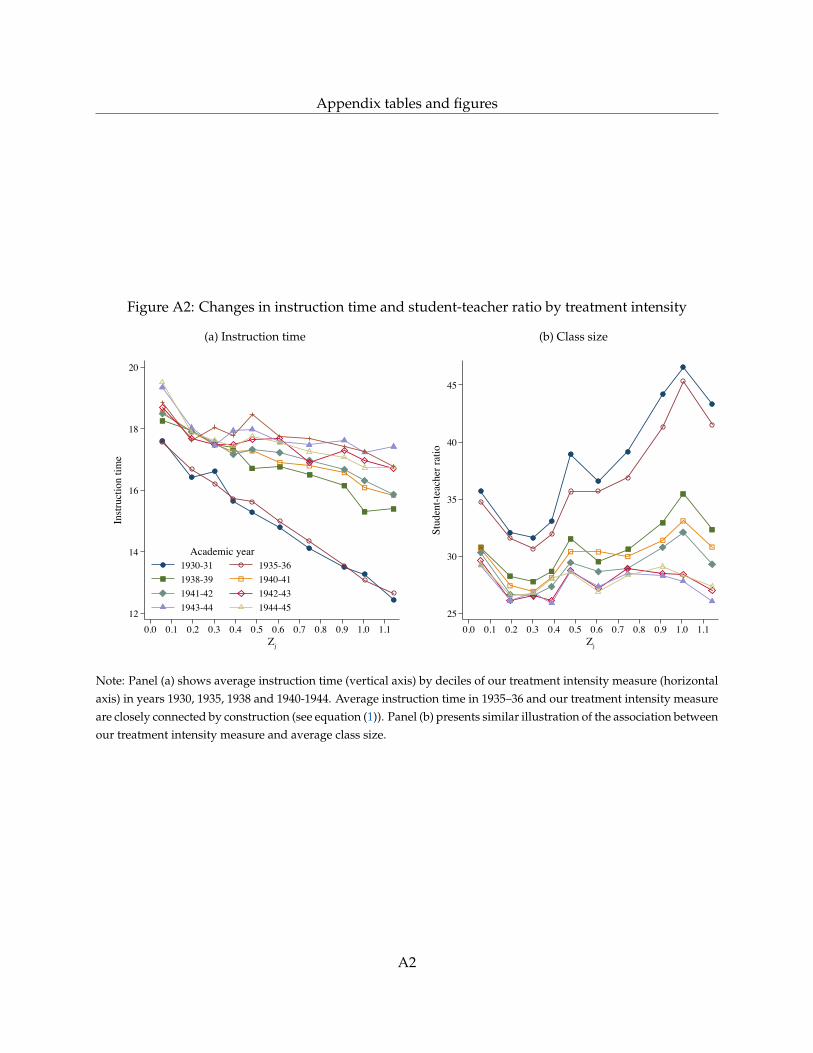
Appendix tables and figures

Figure A2: Changes in instruction time and student-teacher ratio by treatment intensity

(a) Instruction time

12

14

16

18

20

Inst

ruct

ion

time

0.0 0.1 0.2 0.3 0.4 0.5 0.6 0.7 0.8 0.9 1.0 1.1Zj

1930-31 1935-361938-39 1940-411941-42 1942-431943-44 1944-45

Academic year

(b) Class size

25

30

35

40

45

Stud

ent-t

each

er ra

tio

0.0 0.1 0.2 0.3 0.4 0.5 0.6 0.7 0.8 0.9 1.0 1.1Zj

Note: Panel (a) shows average instruction time (vertical axis) by deciles of our treatment intensity measure (horizontalaxis) in years 1930, 1935, 1938 and 1940-1944. Average instruction time in 1935–36 and our treatment intensity measureare closely connected by construction (see equation (1)). Panel (b) presents similar illustration of the association betweenour treatment intensity measure and average class size.

A2

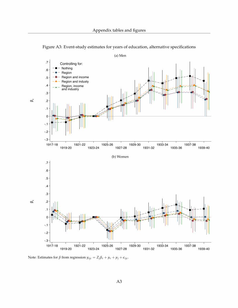
Appendix tables and figures

Figure A3: Event-study estimates for years of education, alternative specifications

(a) Men

-.3

-.2

-.1

0

.1

.2

.3

.4

.5

.6

.7

β c

1917-181919-20

1921-221923-24

1925-261927-28

1929-301931-32

1933-341935-36

1937-381939-40

NothingRegionRegion and incomeRegion and industyRegion, incomeand industry

Controlling for:

(b) Women

-.3

-.2

-.1

0

.1

.2

.3

.4

.5

.6

.7

β c

1917-181919-20

1921-221923-24

1925-261927-28

1929-301931-32

1933-341935-36

1937-381939-40

Note: Estimates for β from regression yijc = Zjβc + µc + µj + εijc.

A3

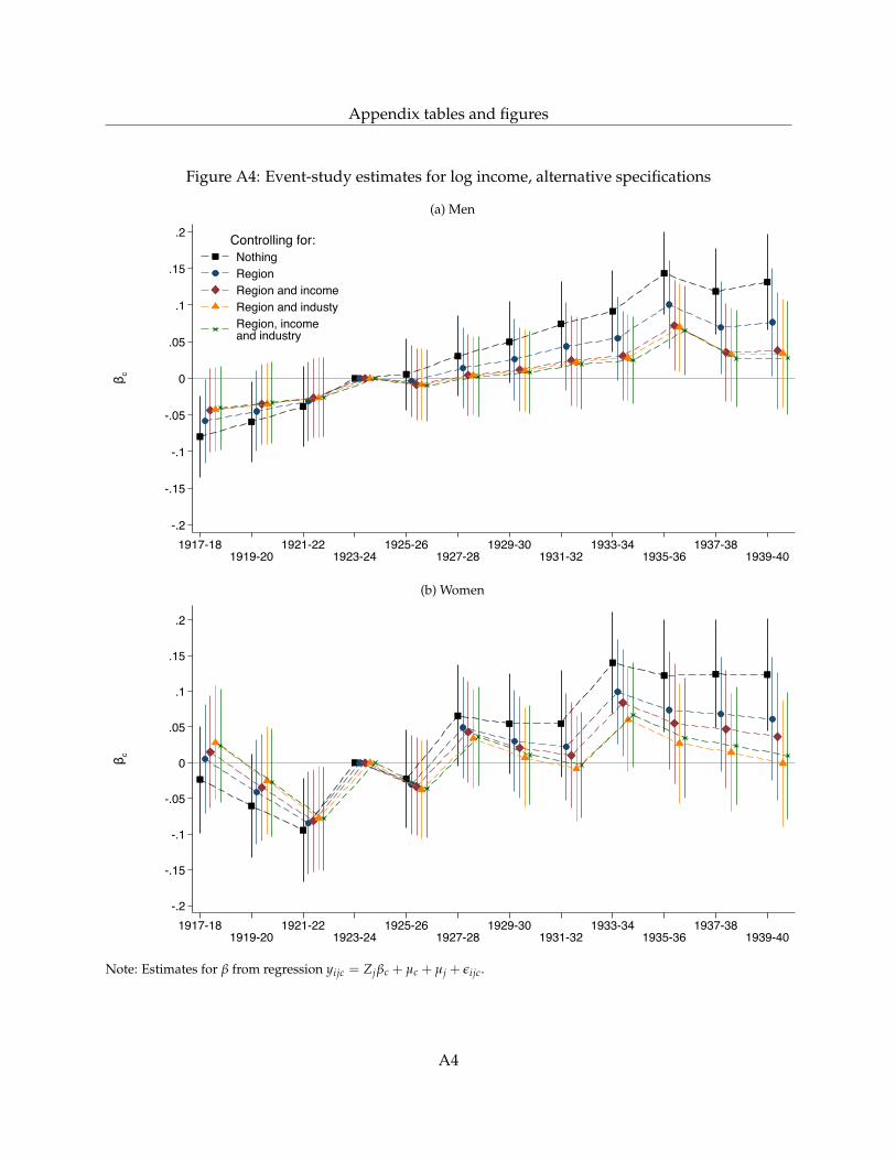
Appendix tables and figures

Figure A4: Event-study estimates for log income, alternative specifications

(a) Men

-.2

-.15

-.1

-.05

0

.05

.1

.15

.2

β c

1917-181919-20

1921-221923-24

1925-261927-28

1929-301931-32

1933-341935-36

1937-381939-40

NothingRegionRegion and incomeRegion and industyRegion, incomeand industry

Controlling for:

(b) Women

-.2

-.15

-.1

-.05

0

.05

.1

.15

.2

β c

1917-181919-20

1921-221923-24

1925-261927-28

1929-301931-32

1933-341935-36

1937-381939-40

Note: Estimates for β from regression yijc = Zjβc + µc + µj + εijc.

A4

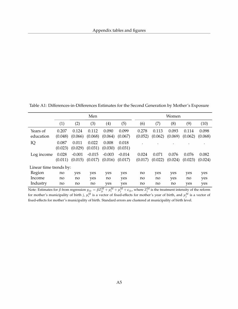
Appendix tables and figures

Table A1: Differences-in-Differences Estimates for the Second Generation by Mother’s Exposure

Men Women

(1) (2) (3) (4) (5) (6) (7) (8) (9) (10)

Years of 0.207 0.124 0.112 0.090 0.099 0.278 0.113 0.093 0.114 0.098education (0.048) (0.066) (0.068) (0.064) (0.067) (0.052) (0.062) (0.069) (0.062) (0.068)IQ 0.087 0.011 0.022 0.008 0.018 . . . . .

(0.023) (0.029) (0.031) (0.030) (0.031)Log income 0.028 -0.001 -0.015 -0.003 -0.014 0.024 0.071 0.076 0.076 0.082

(0.011) (0.015) (0.017) (0.016) (0.017) (0.017) (0.022) (0.024) (0.023) (0.024)

Linear time trends by:Region no yes yes yes yes no yes yes yes yesIncome no no yes no yes no no yes no yesIndustry no no no yes yes no no no yes yes

Note: Estimates for β from regression yijc = βZMjc + µM

c + µMj + εijc, where ZM

j is the treatment intensity of the reformfor mother’s municipality of birth j, µM

c is a vector of fixed-effects for mother’s year of birth, and µMj is a vector of

fixed-effects for mother’s municipality of birth. Standard errors are clustered at municipality of birth level.

A5

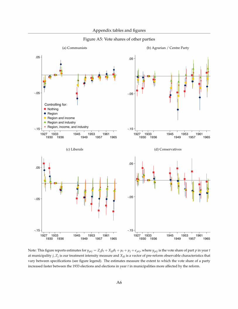
Appendix tables and figures

Figure A5: Vote shares of other parties

(a) Communists

-.15

-.05

.05

19271930

19331936

19451949

19531957

19611965

NothingRegionRegion and incomeRegion and industryRegion, income, and industry

Controlling for:

(b) Agrarian / Centre Party

-.15

-.05

.05

19271930

19331936

19451949

19531957

19611965

(c) Liberals

-.15

-.05

.05

19271930

19331936

19451949

19531957

19611965

(d) Conservatives

-.15

-.05

.05

19271930

19331936

19451949

19531957

19611965

Note: This figure reports estimates for yptj = Zjβt + Xj0θt + µt + µj + εptj, where yptj is the vote share of part p in year tat municipality j, Zj is our treatment intensity measure and Xj0 is a vector of pre-reform observable characteristics thatvary between specifications (see figure legend). The estimates measure the extent to which the vote share of a partyincreased faster between the 1933 elections and elections in year t in municipalities more affected by the reform.

A6

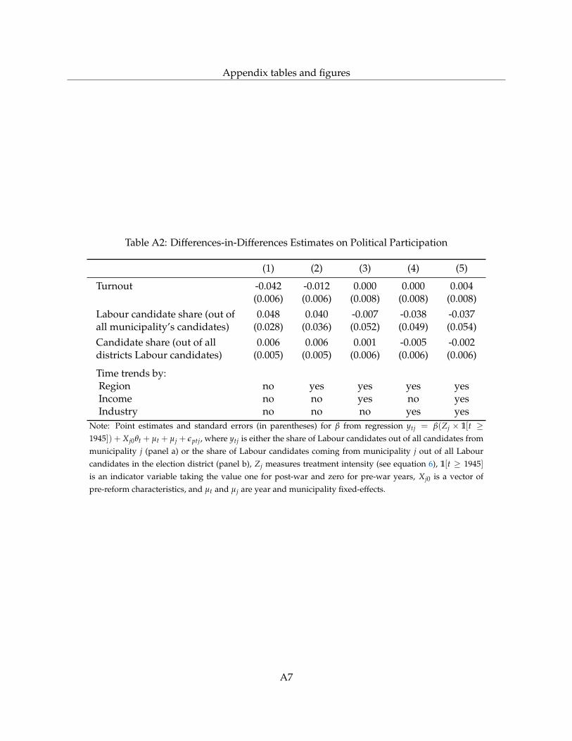
Appendix tables and figures

Table A2: Differences-in-Differences Estimates on Political Participation

(1) (2) (3) (4) (5)

Turnout -0.042 -0.012 0.000 0.000 0.004(0.006) (0.006) (0.008) (0.008) (0.008)

Labour candidate share (out of 0.048 0.040 -0.007 -0.038 -0.037all municipality’s candidates) (0.028) (0.036) (0.052) (0.049) (0.054)Candidate share (out of all 0.006 0.006 0.001 -0.005 -0.002districts Labour candidates) (0.005) (0.005) (0.006) (0.006) (0.006)

Time trends by:Region no yes yes yes yesIncome no no yes no yesIndustry no no no yes yes

Note: Point estimates and standard errors (in parentheses) for β from regression ytj = β(Zj × 1[t ≥1945]) + Xj0θt + µt + µj + εptj, where ytj is either the share of Labour candidates out of all candidates frommunicipality j (panel a) or the share of Labour candidates coming from municipality j out of all Labourcandidates in the election district (panel b), Zj measures treatment intensity (see equation 6), 1[t ≥ 1945]is an indicator variable taking the value one for post-war and zero for pre-war years, Xj0 is a vector ofpre-reform characteristics, and µt and µj are year and municipality fixed-effects.

A7

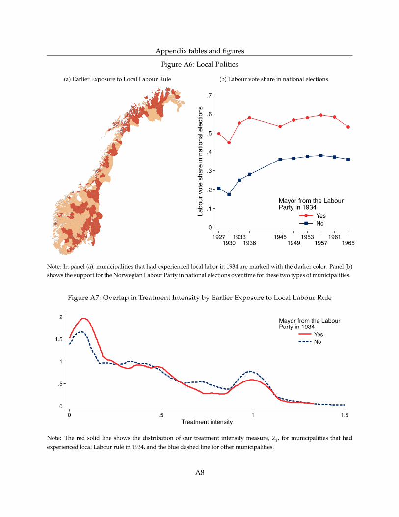
Appendix tables and figures

Figure A6: Local Politics

(a) Earlier Exposure to Local Labour Rule (b) Labour vote share in national elections

0

.1

.2

.3

.4

.5

.6

.7

Labo

ur v

ote

shar

e in

nat

iona

l ele

ctio

ns

19271930

19331936

19451949

19531957

19611965

YesNo

Mayor from the LabourParty in 1934

Note: In panel (a), municipalities that had experienced local labor in 1934 are marked with the darker color. Panel (b)shows the support for the Norwegian Labour Party in national elections over time for these two types of municipalities.

Figure A7: Overlap in Treatment Intensity by Earlier Exposure to Local Labour Rule

0

.5

1

1.5

2

0 .5 1 1.5Treatment intensity

YesNo

Mayor from the LabourParty in 1934

Note: The red solid line shows the distribution of our treatment intensity measure, Zj, for municipalities that hadexperienced local Labour rule in 1934, and the blue dashed line for other municipalities.

A8

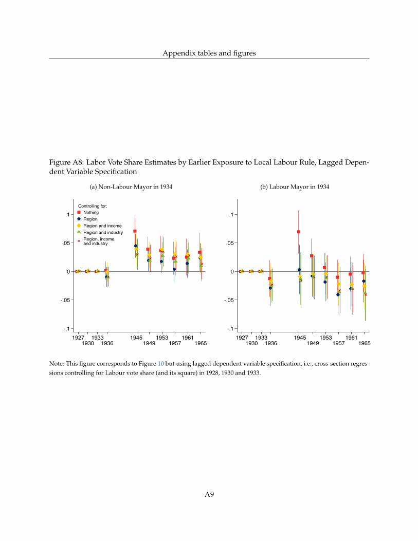
Appendix tables and figures

Figure A8: Labor Vote Share Estimates by Earlier Exposure to Local Labour Rule, Lagged Depen-dent Variable Specification

(a) Non-Labour Mayor in 1934

-.1

-.05

0

.05

.1

19271930

19331936

19451949

19531957

19611965

NothingRegionRegion and incomeRegion and industryRegion, income,and industry

Controlling for:

(b) Labour Mayor in 1934

-.1

-.05

0

.05

.1

19271930

19331936

19451949

19531957

19611965

Note: This figure corresponds to Figure 10 but using lagged dependent variable specification, i.e., cross-section regres-sions controlling for Labour vote share (and its square) in 1928, 1930 and 1933.

A9

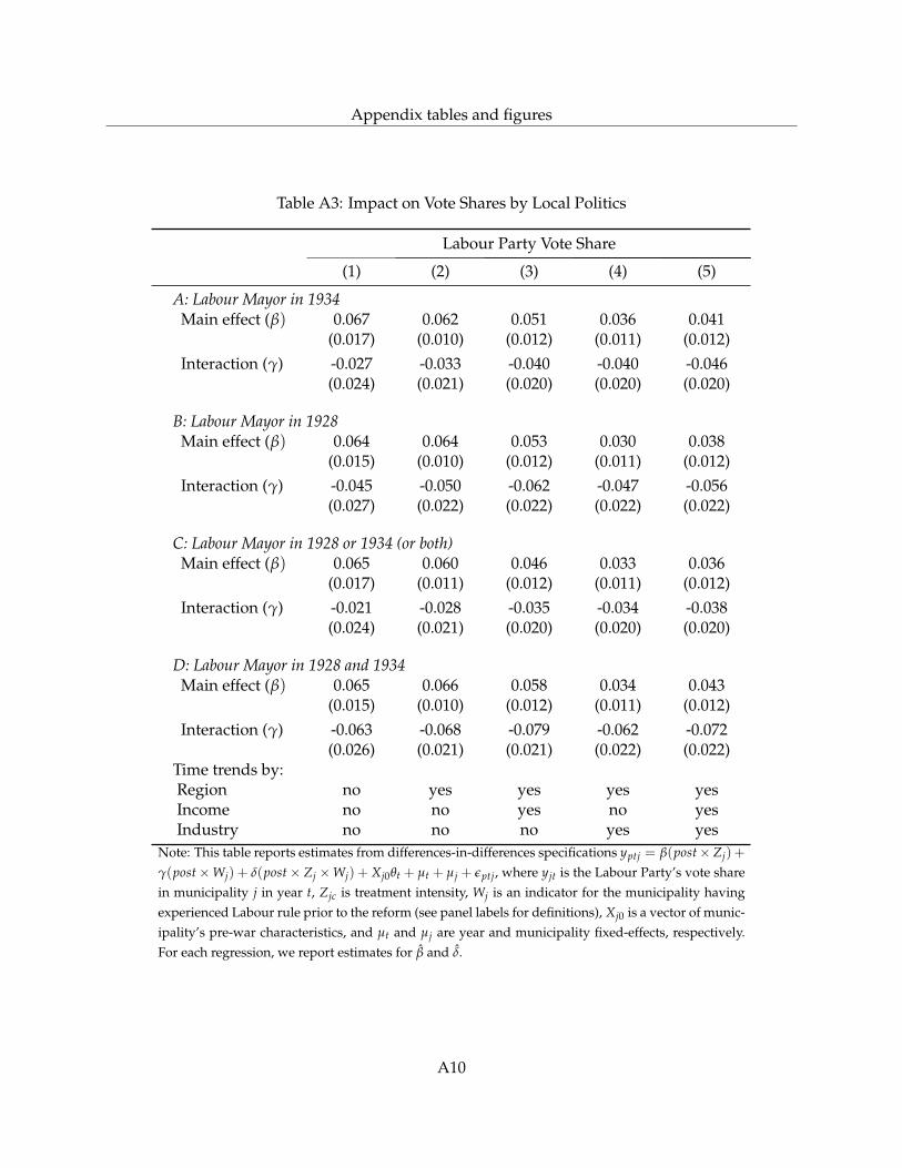
Appendix tables and figures

Table A3: Impact on Vote Shares by Local Politics

Labour Party Vote Share

(1) (2) (3) (4) (5)

A: Labour Mayor in 1934Main effect (β) 0.067 0.062 0.051 0.036 0.041

(0.017) (0.010) (0.012) (0.011) (0.012)Interaction (γ) -0.027 -0.033 -0.040 -0.040 -0.046

(0.024) (0.021) (0.020) (0.020) (0.020)

B: Labour Mayor in 1928Main effect (β) 0.064 0.064 0.053 0.030 0.038

(0.015) (0.010) (0.012) (0.011) (0.012)Interaction (γ) -0.045 -0.050 -0.062 -0.047 -0.056

(0.027) (0.022) (0.022) (0.022) (0.022)

C: Labour Mayor in 1928 or 1934 (or both)Main effect (β) 0.065 0.060 0.046 0.033 0.036

(0.017) (0.011) (0.012) (0.011) (0.012)Interaction (γ) -0.021 -0.028 -0.035 -0.034 -0.038

(0.024) (0.021) (0.020) (0.020) (0.020)

D: Labour Mayor in 1928 and 1934Main effect (β) 0.065 0.066 0.058 0.034 0.043

(0.015) (0.010) (0.012) (0.011) (0.012)Interaction (γ) -0.063 -0.068 -0.079 -0.062 -0.072

(0.026) (0.021) (0.021) (0.022) (0.022)Time trends by:Region no yes yes yes yesIncome no no yes no yesIndustry no no no yes yes

Note: This table reports estimates from differences-in-differences specifications yptj = β(post × Zj) +

γ(post × Wj) + δ(post × Zj × Wj) + Xj0θt + µt + µj + εptj, where yjt is the Labour Party’s vote sharein municipality j in year t, Zjc is treatment intensity, Wj is an indicator for the municipality havingexperienced Labour rule prior to the reform (see panel labels for definitions), Xj0 is a vector of munic-ipality’s pre-war characteristics, and µt and µj are year and municipality fixed-effects, respectively.For each regression, we report estimates for β̂ and δ̂.

A10

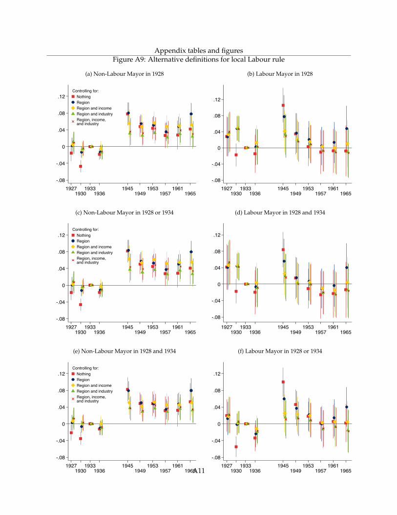
Appendix tables and figuresFigure A9: Alternative definitions for local Labour rule

(a) Non-Labour Mayor in 1928

-.08

-.04

0

.04

.08

.12

19271930

19331936

19451949

19531957

19611965

NothingRegionRegion and incomeRegion and industryRegion, income,and industry

Controlling for:

(b) Labour Mayor in 1928

-.08

-.04

0

.04

.08

.12

19271930

19331936

19451949

19531957

19611965

(c) Non-Labour Mayor in 1928 or 1934

-.08

-.04

0

.04

.08

.12

19271930

19331936

19451949

19531957

19611965

NothingRegionRegion and incomeRegion and industryRegion, income,and industry

Controlling for:

(d) Labour Mayor in 1928 and 1934

-.08

-.04

0

.04

.08

.12

19271930

19331936

19451949

19531957

19611965

(e) Non-Labour Mayor in 1928 and 1934

-.08

-.04

0

.04

.08

.12

19271930

19331936

19451949

19531957

19611965

NothingRegionRegion and incomeRegion and industryRegion, income,and industry

Controlling for:

(f) Labour Mayor in 1928 or 1934

-.08

-.04

0

.04

.08

.12

19271930

19331936

19451949

19531957

19611965A11

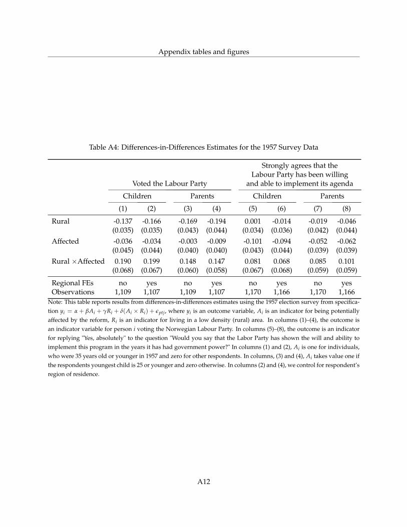
Appendix tables and figures

Table A4: Differences-in-Differences Estimates for the 1957 Survey Data

Strongly agrees that theLabour Party has been willing

Voted the Labour Party and able to implement its agenda

Children Parents Children Parents

(1) (2) (3) (4) (5) (6) (7) (8)

Rural -0.137 -0.166 -0.169 -0.194 0.001 -0.014 -0.019 -0.046(0.035) (0.035) (0.043) (0.044) (0.034) (0.036) (0.042) (0.044)

Affected -0.036 -0.034 -0.003 -0.009 -0.101 -0.094 -0.052 -0.062(0.045) (0.044) (0.040) (0.040) (0.043) (0.044) (0.039) (0.039)

Rural ×Affected 0.190 0.199 0.148 0.147 0.081 0.068 0.085 0.101(0.068) (0.067) (0.060) (0.058) (0.067) (0.068) (0.059) (0.059)

Regional FEs no yes no yes no yes no yesObservations 1,109 1,107 1,109 1,107 1,170 1,166 1,170 1,166

Note: This table reports results from differences-in-differences estimates using the 1957 election survey from specifica-tion yi = α + βAi + γRi + δ(Ai × Ri) + εptj, where yi is an outcome variable, Ai is an indicator for being potentiallyaffected by the reform, Ri is an indicator for living in a low density (rural) area. In columns (1)–(4), the outcome isan indicator variable for person i voting the Norwegian Labour Party. In columns (5)–(8), the outcome is an indicatorfor replying "Yes, absolutely" to the question "Would you say that the Labor Party has shown the will and ability toimplement this program in the years it has had government power?" In columns (1) and (2), Ai is one for individuals,who were 35 years old or younger in 1957 and zero for other respondents. In columns, (3) and (4), Ai takes value one ifthe respondents youngest child is 25 or younger and zero otherwise. In columns (2) and (4), we control for respondent’sregion of residence.

A12