The Malyuzhinets theory for scattering from wedge ...norris/papers/1999... · Wave Motion 29 (1999) 313–340 The Malyuzhinets theory for scattering from wedge boundaries: a review

Wave Motion 29 (1999) 313–340

The Malyuzhinets theory for scattering from wedge boundaries: a reviewA.V. Osipov1,a, A.N. Norrisb,∗

a Institute of Radiophysics, The St. Petersburg State University, Uljanovskaja 1-1, Petrodvorets 198904, Russiab Department of Mechanical and Aerospace Engineering, Rutgers University, 98 Brett Road, Piscataway, NJ 08854-8058, USA

Received 20 December 1996; received in revised form 13 July 1998; accepted 5 August 1998

Abstract

The Malyuzhinets technique is reviewed based on his fundamental papers of the 1950s. Subsequent developments aresurveyed and recent advances are presented. The review is focused around the basic problem of determining the wave fieldscattered from the edge of a wedge of exterior angle 28 with arbitrary impedance conditions on either face. We begin byestablishing a direct relationship between the Sommerfeld integral representation and the Laplace transform. This providesfresh insight into Malyuzhinets’ inferences about functions representable via the Sommerfeld integral and, simultaneously,allows us to prove both the inversion formula for the Sommerfeld integral and the crucial nullification theorem. The specialfunctionsη8(z) andψ8(z) occurring in Malyuzhinets’ theory of diffraction from a wedge-shaped region are described. Basedon this theoretical background we present a detailed derivation of the well-known Malyuzhinets expressions for the wave fielddiffracted by an impedance wedge. An alternative representation of the Malyuzhinets solution as a series of Bessel functionsis also presented that is completely equivalent to the integral form of the Malyuzhinets solution. This permits a descriptionof the wave field in the vicinity of the edge of an impedance wedge, whenkr ≤ 1, and simple expressions are given for thetip values of the field and its first derivatives. The edge valueu0 can be expressed in terms of Malyuzhinets functions, andits magnitude is easily evaluated if the impedances of the wedge faces are purely imaginary. Thus,|u0| ≤ π/8 with equalityonly for a wedge with Neumann boundary conditions.c©1999 Elsevier Science B.V. All rights reserved.

1. Introduction

Diffraction from a wedge is a well covered topic, dating back over a century; see Refs. [1,2] for early citationsby Sommerfeld, Poincare, MacDonald, and others. Corresponding solutions relevant to the Dirichlet or Neumannboundary conditions on the wedge faces are presented in more detail in Refs. [1–9]. The generalised problemwith impedance boundary conditions on the faces was solved by Malyuzhinets in his D.Sc. Dissertation [10], anddescribed in a series of classic papers [11–14], culminating in the concise solution outlined in his 1958 paper [15].His solution was deduced in the form of a Sommerfeld integral with an integrand involving a new special functionψ8(z). Malyuzhinets later gave a short review of the method in Ref. [16], his only paper published in a non-Russian

∗ Corresponding author; e-mail: [email protected] Now with German Aerospace Center, DLR Institute of Radio Frequency Technology, P.O. Box 1116, D-82230 Wessling, Germany. E-mail:

[email protected]

0165-2125/99/$ – see front matterc©1999 Elsevier Science B.V. All rights reserved.PII: S0165-2125(98)00042-0

314 A.V. Osipov, A.N. Norris / Wave Motion 29 (1999) 313–340

journal. His works extended and transformed the intuitive Sommerfeld approach into an elegant formal procedurethat exploits basic concepts of mathematical analysis rather then constructing images of a real source in a fictitiousbranched Riemann space. Williams [17] independently solved the problem for a wedge with the same impedance oneach face in terms of the Sommerfeld integral and a double gamma function, whereas Senior [18] using the Laplacetransform provided a solution of an electromagnetic diffraction problem involving a wedge with finite conductivity.

Further contributions to the Malyuzhinets theory were made by Tuzhilin who developed a theory of relatedfunctional equations [19–21] and demonstrated the possibility of extending the Malyuzhinets approach to moresophisticated boundary conditions [22] (the solution for the particular case of a thin elastic semi-infinite plate waspublished in [23–25]). Diffraction of a transient scalar wave by an impedance wedge was considered by Sakharovaand Filippov in [26,27], and the result was expressed in terms of the special functionψ8(z) occurring at theMalyuzhinets theory. In [27] Filippov gave also a complete uniform asymptotic expansion for the far-field scatteredby an impedance wedge.

Zavadskii and Sakharova [28] developed the first numerical procedures for computing the Malyuzhinets specialfunction and deduced some useful analytical representations [29,30]. Numerical calculations of the functionψπ(α),relevant to a screen, were discussed by Volakis and Senior [31], and Hongo and Nakajima [32] derived an expansionfor the general functionψ8(α) by using Chebyshev polynomials. Herman et al. [33] provided simple analyticexpressions forψ8(α) for small and large arguments. Osipov presented more refined approximations accurateto better than 0.01% over the whole complexα plane by combining direct numerical integration in the integralrepresentation ofψ8(α) given by Zavadskii and Sakharova [29] with summation of a new series representationof the Malyuzhinets function [34]. Further contributions are authored by Aidi and Lavergnat [35] who utilisedthe results of [34] and also proposed alternative methods permitting to save computational times. The authors of[36] have proposed to evaluate the Malyuzhinets function by rearranging its integral representation and performingnumerical integration according to trapezoidal rule, in contrast to Laguerre quadrature employed in [34].

Malyuzhinets’ solution, having the form of a Sommerfeld integral, is perfectly suited for the purpose of subsequentfar-field analysis. In contrast, the analysis of the near-field behaviour requires an alternative representation for thesolution. This was achieved by Budaev and Petrashen’ [37] who found series representations of the field diffractedby a wedge with equal face impedances, and by Osipov [38] who deduced the series solution for the general caseof arbitrary face impedances.

Depending upon the value of the vertex angle, the model of an impedance wedge uniformly includes a variety ofcanonical geometries, including an imperfect half-plane, a flat surface with an impedance step, and an impedancehorn. Many papers have appeared dealing with both electromagnetic and acoustic applications in these configura-tions. For instance: plane wave scattering from an impedance half-plane [39,40]; radiation of a line source at the tipof an absorbing wedge [41–46]; Green’s functions [47,48]; edge waves [49]; diffraction of surface [45,50,51], plane[45,52–59], cylindrical [45,47,48,60–64], and transient scalar [26,27] waves by an impedance wedge of arbitraryangle. The corresponding mathematical solution for the impedance wedge can therefore serve as a universal basisfor treating scattering and diffraction problems. However, the lack of comprehensive publications of Malyuzhinets’results and the apparent complexity of his solution, caused many researchers and engineers to utilise differentmathematical approaches which proved to be either less efficient for this class of diffraction problems, such asthe Kontorovich–Lebedev transform [65] and the method of eigenfunction expansion [37,66], or fundamentallyrestricted to rectangular geometries, such as the Wiener–Hopf technique [67], or the methods described in [68–71]. In this paper we restrict ourselves to the Malyuzhinets method and the arbitrary-angled impedance wedge,and therefore this review does not include a great many publications dealing with the Wiener–Hopf method andrectangular geometries (for a detailed discussion of this subject see [72–74]).

The purpose of this paper is not to derive the solution for the impedance wedge, which is well known, but todiscuss the key points of the Malyuzhinets theory, emphasizing its fundamental character and the physical clarity ofits consequences. We believe this is important for further understanding of wave phenomena because Malyuzhinets’approach provides a powerful means for tackling one of the basic questions of wave theory, that is, the diffractionby edged obstacles. It should be pointed out that this paper gives our own insights into this theory, which almost

A.V. Osipov, A.N. Norris / Wave Motion 29 (1999) 313–340 315

certainly differs from the original and highly unconventional concepts introduced by Malyuzhinets, which basicallyutilised sophisticated geometrical constructions rather than algebraic manipulations [10]. This review is intended todemonstrate that the key principles of Malyuzhinets’ method can be explained in a simple way, easily understandableby Wiener–Hopf people, in terms of certain well-known facts from the theory of functions of a complex variable.We hope that this will satisfy the demand for more detailed explanations of the method that has arisen decades afterthe publication of Malyuzhinets’ famous papers of the 50’s (see, for example, [75]).

The paper is organised as follows. Section 2 is devoted to foundations of the Malyuzhinets theory. It starts (Section2.1) with two key propositions in Malyuzhinets’ method: the inversion formula for the Sommerfeld integral and thenullification theorem [13]. Unlike Malyuzhinets’ original papers, this section presents an alternative derivation ofthese identities which makes use of the relationship between the Sommerfeld and Laplace integral representations.This allows us to interpret the foundations of the Malyuzhinets method as a direct consequence of the Watson lemmaand the Liouville theorem, the two basic statements of the Laplace transform theory. In this section we follow theapproach presented in [76]. The properties of the Sommerfeld integral are also discussed in [45,66].

Section 2.2 describes a special functionη8(z) relevant to the solution of the radiation problem when the wave fieldis excited within a wedge-shaped region by sources distributed on its boundaries [11,12]. Section 2.3 is devoted tothe special functionψ8(z) that arises from the theory of diffraction by a wedge with impedance boundary conditions[15]. These two sections gather together almost all the known analytical results concerning the functionsη8(z) andψ8(z) presented in the literature so far.

Section 3 addresses the derivation of Malyuzhinets’ solution for diffraction from an impedance wedge. We providea detailed and complete derivation of the relevant transform function, using only the Fourier transformation. Thissection may be considered as our interpretation of the procedure only briefly outlined in the famous Malyuzhinetspaper [15]. Section 3 concludes with a closed-form expression for the transform function in terms of the specialfunctionψ8 introduced in Section 2.3.

Section 4 of the paper deals with another form of the solution for an impedance wedge. We show in Section 4.1how the Malyuzhinets solution deduced initially as a Sommerfeld integral can be transformed into a series in termsof Bessel functions. We present an alternative representation which is exact and completely equivalent to the initialSommerfeld integral, and in agreement with the well-known series solution for wedges with ideal boundaries.

The series form of the solution has some advantages over the Sommerfeld integral for analysing the wave fieldin the near-and intermediate zones wherekr is no longer a large parameter. On the basis of the series representationwe deduce simple expressions showing how the singular components of the wave field behave close to the edge ofan impedance wedge.

In Section 4.2 we study the tip value of the field, providing both computational results and simple analyticalformulae. These results have proven useful in the far-field analysis of the Malyuzhinets solution.

Because of the space limitations, this paper does not address topics related to the far-field analysis of the Ma-lyuzhinets solution. This is the subject of a separate paper [77], which discusses the far-field specifically and providessome new results for the diffraction coefficient.

2. The foundations

2.1. The Sommerfeld integral and its inversion

We are concerned with solutions to the Helmholtz equation

∂2u

∂r2+ 1

r

∂u

∂r+ 1

r2

∂2u

∂φ2+ k2u = 0, (1)

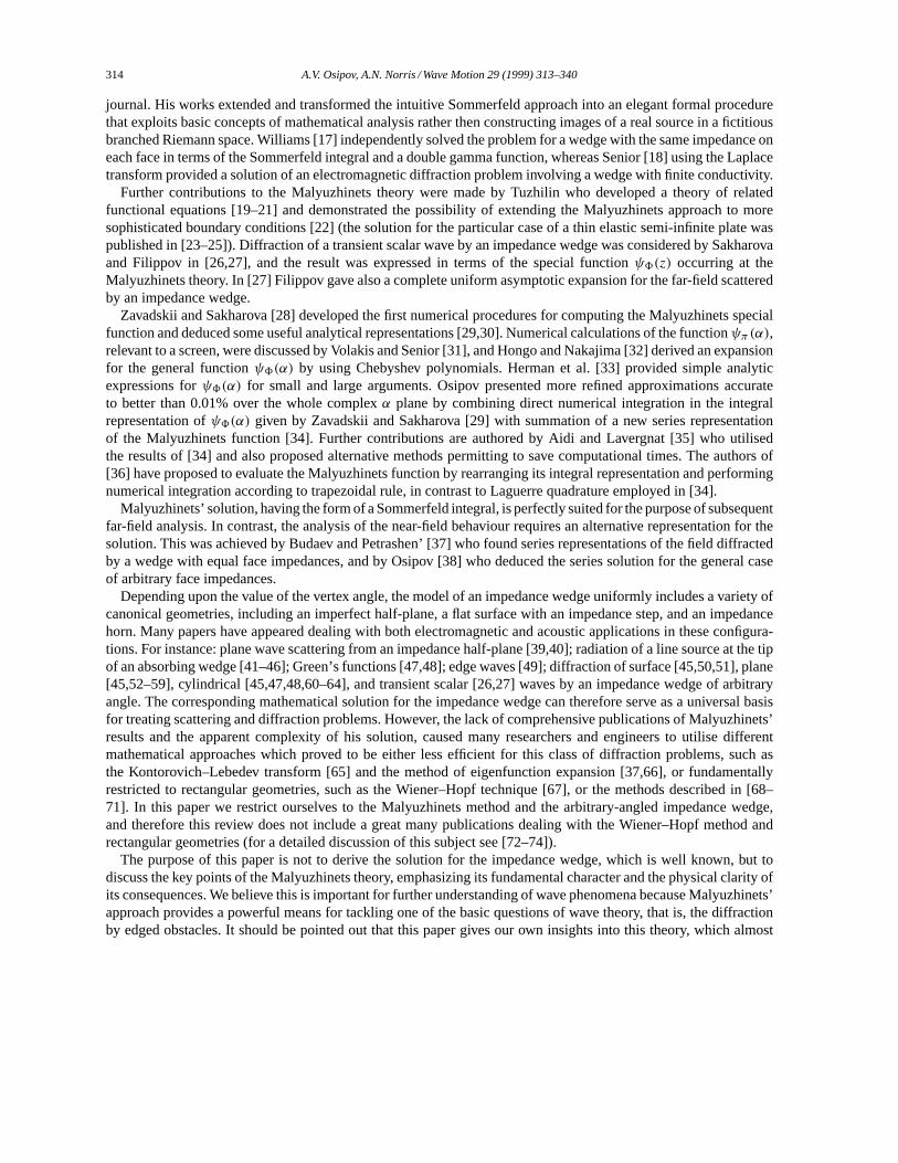
within a wedge-shaped region 0< r < ∞, |φ| ≤ 8, see Fig. 1. Herek = ω/c andc is the wave speed. The


Fig. 1. The geometry.

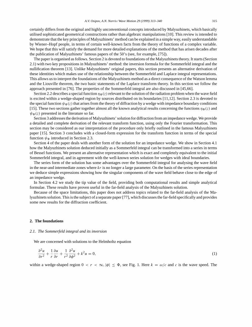
Fig. 2. Integration contours of the Sommerfeld integral.

functionu(r, φ) represents either the sound pressure in acoustics or a component of the electric/magnetic field inelectromagnetics.

Within the framework of the Malyuzhinets method the solution to the problem of diffraction by a wedge-shapeddomain is sought in the form of an integral

u(r, φ) = 1

2π i

∫γ

e−ikr cosαS(α + φ)dα, (2)

taken over the contourγ = γ+⋃γ− in the spectral complex planeα (Fig. 2). Hereγ+ is a loop in the upper half of

the complexα-plane, beginning atπ/2+ i∞, ending at−3π/2+ i∞, with Imα lying above an arbitrary minimum,such that no singularities of the integrand occur withinγ+ for all |φ| ≤ 8. The contourγ− is the image ofγ+ underinversion about the originα = 0. The ends of the integration contours are located in those portions of the complexα-plane (hatched in Fig. 2) where Im(k cosα) < 0 to ensure convergence of the integral.

The integral of the form (2) has been introduced by Sommerfeld in his famous paper of 1896 on diffraction of anelectromagnetic wave from a perfectly conducting half-plane. For arbitrary spectral functionS(α) the Sommerfeldintegral (2) satisfies the Helmholtz equation (1) and can be interpreted as an expansion of the wave field into a planewave spectrum.

The symmetry ofγ+ andγ− yields

u(r, φ) = 1

2π i

∫γ+

e−ikr cosα[S(α + φ)− S(−α + φ)] dα, (3)


implying that the integral (2) is invariant under the transformationS(α) → S(α)+ const. By appropriate choice ofthis constant we can set, without loss of generality,

S(i∞) = −S(−i∞), (4)

which will be assumed hereinafter. This limiting value ofS in (4) is related to the potential function at the wedgetip. Thus, asr → 0 we may let the contourγ+ recede towards i∞, in the limit obtaining simply

u(0, φ) = 2iS(i∞). (5)

The Sommerfeld integral representation (3) can be expressed in a concise form

F(r) = 1

π i

∫γ+

e−ikr cosαf (α)dα, (6)

with F(r) = u(r, ϕ) and 2f (α) = S(α + ϕ) − S(−α + ϕ), representing at a given value of the parameterϕ thepotential function and the odd part of the transform function, respectively. Thus, the key point of the Malyuzhinetstheory is to prove that the functionsF(r) to be sought can indeed be represented as (6) withf (α) being an oddfunction ofα, analytic inside the contourγ+ and bounded at infinity Imα = +∞.

To this end, deform the integration contourγ+ into a new contourγ+ (Fig. 2) lying entirely within the strip onthe complexα-plane in which Im(k cosα) > 0, and which is defined by the equation Re(−ik cosα) = σ , whereσ is a positive constant. Along this latter contour the exponent function in (6) is oscillating and bounded, whichensures the convergence of the integral so far as the bounded transform functionsf (α) are concerned. Notice thatno singular points of the functionf (α) may fall between the contoursγ+ andγ+ because of analyticity off (α)inside the loopγ+. Thus, one has

F(r) = 1

π i

∫γ+

e−ikr cosαf (α)dα. (7)

Next, changing the integration variable according top = −i cosα transforms the expression (7) into

F(r) = 1

2π i

∫ σ+i∞

σ−i∞eprQ(p)dp, (8)

with

Q(p) = 2f (α)

ik sinα. (9)

Eq. (8) represents an inverse Laplace transform, and its inversion can therefore be achieved by the direct Laplacetransform

Q(p) =∫ +∞

0e−prF (r)dr, (10)

or, in terms of the variableα,

f (α) = ik

2sinα

∫ +∞

0eikr cosαF (r)dr. (11)

Expressions (7) and (11) are completely equivalent to those of the Laplace transform, (8) and (10), respectively.The analyticity of the transform functionf (α) inside the contourγ+ results from that of the Laplace transformfunctionQ(p) to the right of the contour Rep = σ [78]. The fact thatf (α) is an odd function ofα is dictated bythe form of Eq. (11). Indeed, forF(r) = O[exp(−br)] with b > 0 whenr → +∞, which is true for outgoing


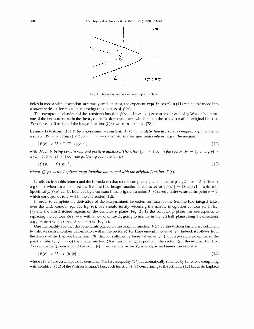
Fig. 3. Integration contours in the complexp plane.

fields in media with absorption, arbitrarily small at least, the exponent exp(ikr cosα) in (11) can be expanded intoa power series in ikr cosα, thus proving the oddness off (α).

The asymptotic behaviour of the transform functionf (α) as Imα → +∞ can be derived using Watson’s lemma,one of the key statements in the theory of the Laplace transform, which relates the behaviour of the original functionF(r) for r → 0 to that of the image functionQ(p) when|p| → +∞ [78]:

Lemma 1 (Watson).Let δ be a non-negative constant,F(r) an analytic function on the complexr-plane withina sectorRδ = {r : | argr| ≤ δ,0< |r| < +∞} in which it satisfies uniformly inargr the inequality

|F(r)| < M|r|−1+a exp(b|r|), (12)

with M,a, b being certain real and positive numbers. Then, for|p| → +∞ in the sectorPδ = {p : | argp| <π/2 + δ,0< |p| < +∞} the following estimate is true

|Q(p)| = O(|p|−a), (13)

whereQ(p) is the Laplace image function associated with the original functionF(r).

It follows from this lemma and the formula (9) that on the complexα-plane in the strip argk− π − δ < Reα <argk + δ when Imα → +∞ the Sommerfeld image function is estimated as|f (α)| = O{exp[(1 − a)Im α]}.Specifically,f (α) can be bounded by a constant if the original functionF(r) takes a finite value at the pointr = 0,which corresponds toa = 1 in the expression (12).

In order to complete the derivation of the Malyuzhinets inversion formula for the Sommerfeld integral takenover the wide contourγ+, see Eq. (6), one should justify widening the narrow integration contourγ+ in Eq.(7) into the crosshatched regions on the complexα-plane (Fig. 2). In the complexp-plane this corresponds toreplacing the contour Rep = σ with a new one, sayL, going to infinity in the left half-plane along the directionsargp = ±(π/2 + ε) with 0< ε < π/2 (Fig. 3).

One can readily see that the constraints placed on the original functionF(r) by the Watson lemma are sufficientto validate such a contour deformation within the sectorPδ for large enough values of|p|. Indeed, it follows fromthe theory of the Laplace transform [78] that for sufficiently large values of|p| (with a possible exception of thepoint at infinity |p| = ∞) the image functionQ(p) has no singular points in the sectorPδ if the original functionF(r) in the neighbourhood of the point|r| = +∞ in the sectorRδ is analytic and meets the estimate

|F(r)| < M1 exp(b1|r|), (14)

whereM1, b1 are certain positive constants. The last inequality (14) is automatically satisfied by functions complyingwith condition (12) of the Watson lemma. Thus, each functionF(r) conforming to the estimate (12) has as its Laplace


image a functionQ(p) which is both vanishing according to (13) and analytic within the sectorPδ for |p| → +∞(note thatQ(p) may have singular points in the sectorPδ, but only at finite distances from the originp = 0).

It is now straightforward to formulate the Malyuzhinets theorem on the inversion of the Sommerfeld integral[23]. In fact, this theorem results from the foregoing as a direct consequence of the Watson lemma.

Theorem 2(Inversion formula for the Sommerfeld integral).Let M,M1, a, b, δ be positive numbers, and letε bea number satisfying0 < ε < inf (δ, π). Let F(r) be an analytic function in the entire sectorRδ in which itsatisfies uniformly inargrthe inequality(12):

|F(r)| < M|r|−1+a exp(b|r|).Consider the Sommerfeld integral(6) over the contourγ+ that goes fromα = argk + ε + i∞ to α = argk −π − ε+ i∞. Then, among odd functionsf (α), which are analytic on and within the contourγ+ except at infinity,and which may not grow likeexp(Im α) or faster as Im α → +∞,

(i) there exists one and only one solutionf (α) to the integral equation(6);(ii) for Im(k cosα) > b this solution is represented by the inversion formula(11);

(iii) inside the contourγ+ when Im α → +∞ it is estimated by the inequality

|f (α)| < M1 exp[(1 − a)Im α].

An important consequence of this theorem is that there are functionsF(r) that can be represented as the Som-merfeld integral (7) over the narrow contourγ+ but not if the integration is performed over the wide contourγ+.For example, solutions of wave problems involving point sources, like the Green function, possess a singularity atthe source location point and therefore can not be represented as the conventional integral (6) which becomes in thiscase divergent. However, it is still possible to use the modified integral (7) to represent such solutions (see [48]).

To conclude our discussion on the foundations of the Malyuzhinets theory, let us take a look at another keystatement of this theory: the nullification theorem for the Sommerfeld integral [13].

Theorem 3(Nullification of the Sommerfeld integral).Consider the homogeneous integral equation

1

π i

∫γ+

e−ikr cosαf (α)dα = 0. (15)

Let the asymptotic behaviour of the functionf (α) when Im α → +∞ be bounded by the estimate|f (α)| ≤O[ exp(D Im α)]whereD denotes a real number, positive or negative. Then, among odd functionsf (α), analytic onand within the contourγ+ except at the point at infinity,

(i) there exists only the trivial solutionf (α) ≡ 0 to theEq. (15) if D ∈ (−∞,1);(ii) otherwise, forD ≥ 1 the homogeneous integral equation(15) is satisfied by any trigonometric polynomial

expression of the formf (α) = sinα∑nm=1Cm cosm−1α where Cm are arbitrary constants, andn means

the integer part ofD.This theorem is used to solve equations that arise from applying the Sommerfeld integral to boundary conditions

involving higher-order field derivatives with respect to the space coordinates. The examples are the boundaryconditions simulating the presence of a membrane or a thin elastic plate in an acoustic media, or a thin non-metallicsheet in problems of electromagnetic diffraction.

Malyuzhinets proved the nullification theorem by integrating by parts in Eq. (15), thus reducing (15) to a formwhich permits the application of the inversion formula withF(r) ≡ 0. It is shown below that the nullificationtheorem follows from the so-called extended Liouville theorem (see, for example, [79], p. 84).

Consider Eq. (15) in terms of the complex variablep = −ik cosα, related to the Laplace transform. Then onehas the equation∫

L

eprQ(p)dp = 0, r > 0, (16)


in which the contourL is the image of the contourγ+ in the complexp-plane (Fig. 3). Eq. (16) implies thatQ(p)has no singular points inside the contourL. On the other hand by the definition of the contourγ+ the functionQ(p)must be analytic to the right of the contourL as well, since this area corresponds to the interior ofγ+. Thus, thefunctionQ(p) is an entire function of the complex variablep over the whole complexp-plane.

If the asymptotic behaviour off (α) is estimated withD < 1, then according to its definition in Eq. (9)Q(p) →0 as|p| → +∞. The further application of Liouville’s theorem, which states that a bounded entire function is aconstant, uniquely determinesQ(p) to be identically zero. Alternatively, ifD ≥ 1, then in the vicinity of the pointat infinity the functionQ(p) behaves like O(|p|D−1), and according to the extended Liouville theorem the functionQ(p) is a polynomial inp of degree not exceeding the integer part of the differenceD− 1. In terms of the variableα this immediately givesf (α) = sinα

∑nm=1Cm cosm−1α, which completes the proof of the nullification theorem.

2.2. The functionη8

We begin with the functionη8 introduced by Malyuzhinets in 1955 [11] for solving the problem of acousticradiation from the faces of a wedge undergoing prescribed normal velocity. The normal velocity into the fluid oneither face is

v = ± i

ωρr

∂u

∂φ(r, φ)

∣∣∣∣φ=±8

,

whereρ is the fluid density. Therefore, we first consider the boundary condition

i

kr

∂u

∂φ(r, φ) = 1, φ = 8, 0< r < ∞,

i

kr

∂u

∂φ(r, φ) = 0, φ = −8, 0< r < ∞. (17)

We begin by noting that the Sommerfeld transform ofF = 1 isf (α) = −12 tanα, or

1

2π i

∫γ

e−ikr cosα tanα dα = −2, (18)

which can be deduced by first using Eq. (3) followed by the change of variable cosα = x. This permits us to rewritethe boundary conditions (17) in the form

1

2π i

∫γ+

e−ikr cosα[S(α +8)+ S(−α +8)+ secα] sinα dα = 0,

1

2π i

∫γ+

e−ikr cosα[S(α −8)+ S(−α −8)] sinα dα = 0. (19)

According to the nullification theorem, the integrals in Eq. (19) vanish for allr > 0 if and only if the integrandfunctions vanish for allα. PuttingS(α) = η8(α +8) yields the pair of functional equations

η8(α + 28)+ η8(−α + 28) = −secα, η8(α)+ η8(−α) = 0, (20)

the latter implying thatη8(α) is an odd function of its argument. The former equation may therefore be written as

η8(α − 28)− η8(α + 28) = secα. (21)

The equation in (21) can be solved using the integral transformation [15]

η8(α) =∫ i∞

−i∞e−itαG(t)dt, G(t) = − 1

2π

∫ i∞

−i∞eitαη8(α)dα, (22)


which differs from the conventional Fourier transform only by a change of variables. Multiplying both sides of Eq.(21) by exp(itα) and integrating, yields

G(t) = −1

4π i sin (28t)

∫ i∞

−i∞eitα

cosαdα = −

[4 sin(28t) cos

(πt

2

)]−1

, (23)

and therefore,

η8(α) = −1

4

∫ +i∞

−i∞e−itα

sin(2t8) cos(πt/2)dt. (24)

This is the fundamental identity which we will use later for the problem with impedance boundary conditions.Eq. (24) may be rewritten [29]

η8(α) = −1

2

∫ ∞

0

sinh(sα)ds

cosh(12πs) sinh(28s)

. (25)

The functionη8 has the additional properties

η8

(α + π

2

)+ η8

(α − π

2

)= − π

48tan

(πα48

), (26)

η8(α +8)+ η8(α −8) = η8/2(α), (27)

which follow from (25) and the integral identities, valid for|Reα| < 1,∫ ∞

0

cosh(tα)

coshtdt = π

2sec

(πα2

),

∫ ∞

0

sinh(tα)

sinhtdt = π

2tan

(πα2

). (28)

Eq. (25) implies thatη8(α) is analytic for|Reα| < 12π + 28. It may be continued to values ofα outside of this by

repeated use of the functional relation (21). Therefore,η8(α) possesses only simple poles and no branch cuts, andthe poles are at the points

α = ±αnm, αnm = π

2(2m− 1)+ 28(2n− 1), (29)

for n,m = 1,2,3, . . . , with residues(−1)m−1, implying [11]

η8(α) =∞∑l=1

∞∑q=1

(−1)l+12α

α2 − [ π2 (2l − 1)+ 28(2q − 1)]2. (30)

This simplifies further when8 = nπ/(4m), wheren/m is rational and irreducible: thus [15],

ηnπ/4m(α) = 1

n

m∑k=1

n∑l=1

(−1)l1

2tan

[α

2n+ 1

2a(k, l)

], n odd,

ηnπ/4m(α) = 1

n

m∑k=1

n∑l=1

(−1)l1

π

[αn

+ a(k, l)]

cot[αn

+ a(k, l)], n even, (31)

where

a(k, l) = π

2

(2l − 1

n− 2k − 1

m

). (32)


For example [11,32],

ηπ/4(α) = −1

2tan

α

2, ηπ/2(α) = 2α − π sinα

4π cosα,

η3π/4(α) = −1

6tan

(α6

)(3 + 2 cos(α/3)

1 + 2 cos(α/3)

),

ηπ (α) = (√

2 − cos(α/2)) sin(α/2)− α/π

4 cosα.

Returning to the original problem, we can now consider the case when the faces each have constant prescribednormal velocitiesv± onφ = ±8. The solution is given by (2) with

S(α) = ρcv+η8(α +8)+ ρcv−η8(α −8).

The value ofη8(i∞) is readily deduced from (26) asη8(i∞) = −iπ/(88), which together with (5) implies thatthe wave field at the edge, the tip pressure, is [11]

u(0, φ) = π

48ρc(v+ + v−). (33)

Malyuzhinets [12] derived further results concerning the solution for vibrating faces. Among them is the remarkablefact that the acoustic power radiated from the faces in the region 0< r < r1 is

ρc

2(|v+|2 + |v−|2)r1,

for large values ofr1. This is the same power predicted on the basis of the plane wave approximationu(r,±8) =ρcv±, and implies that the edge causes no additional radiation. Malyuzhinets also considered the more generalsituation where the faces vibrate with velocity proportional to exp(−ikr cosβ), β constant. He introduced anddiscussed the generalised functionη∗

8(α, β) [12] which reduces toη8(α) whenβ = 12π .

2.3. The functionψ8

The Malyuzhinets functionψ8 [15] is closely related toη8 mathematically, although the physical interpretationis not as immediate. We will return to this later, but for the moment defineψ8 as

ψ8(α) = exp

[∫ α

0η8(t) dt

]. (34)

It is an even function of its argument and it follows from Eqs. (25) and (34) on carrying out the integration withrespect tot that [29]

ψ8(α) = exp

[−1

2

∫ +∞

0

cosh(tα)− 1

t cosh(tπ/2) sinh(2t8)dt

], (35)

|Reα| < 12π + 28. It may be continued outside this strip by using any of the functional properties [15]:

ψ8(α + 28)

ψ8(α − 28)= cot

(α2

+ π

4

), (36)

ψ8

(α + π

2

)ψ8

(α − π

2

)= ψ2

8

(π2

)cos

(πα48

), (37)

ψ8(α +8)ψ8(α −8) = ψ28(8)ψ8/2(α). (38)


These are immediate consequences of Eqs. (21) and (26), and the identity∫ α

0seczdz = log tan

(α2

+ π

4

). (39)

Moreover,ψ8(α) = ψ8(α)where the bar denotes a complex conjugate, and this together with its evenness propertyand the functional relations (36) and (37) implies thatψ8(α) can be found for any complex-valuedα once it isknown in the fundamental domain 0≤ Reα ≤ inf (1

2π,28), Imα ≥ 0.As a function of the complex variableα the Malyuzhinets functionψ8(α) has zeros atα = ±αnm for n =

1,2,3, . . . , m = 1,3,5, . . . and poles form = 2,4,6, . . . . Therefore, using Eqs. (30) and (34)

ψ8(α) =∞∏l=1

∞∏k=1

{1 − α2

[ π2 (2l − 1)+ 28(2k − 1)]2

}(−1)l+1

. (40)

This again simplifies for8 = πn/(4m). Using Eq. (31), we find that [15],

ψπn/4m(α) =m∏k=1

n∏l=1

(cos [12a(k, l)]

cos [12a(k, l)+ α2n ]

)(−1)l

, if n is odd,

ψπn/4m(α) =m∏k=1

n∏l=1

exp

[(−1)l

π

∫ a(k,l)+α/n

a(k,l)

u cotudu

], if n is even, (41)

wherea(k, l) are defined in (32). Specific examples are [15],

ψπ/4(α)= cosα

2, ψ3π/4(α) = 4

3cos

α

6− 1

3secα

6,

ψπ/2(α)= exp

(1

4π

∫ α

0

2t − π sint

costdt

),

ψπ(α)= exp

[− 1

8π

∫ α

0

π sint − 2√

2π sin(t/2)+ 2t

costdt

].

The Malyuzhinets function can also be represented as follows [34,38]:

ψ8(z) = 1√2ψ8

(π2

)exp

{−is

πz

88+ I (sz,8)

}. (42)

Heres = sign(Im z) and

I (w,8) =∞∑k=1

(−1)k+1

{eiπkw/(28)

2k cos [π2k/(48)]+ ei(2k−1)w

(2k − 1) sin [28(2k − 1)]

}. (43)

The series in Eq. (43) converges absolutely if Imw > 0. For |Im z| � 1 the termI (w,8) in Eq. (42) becomesnegligibly small, which leads to the asymptotic formula

ψ8(z) = 1√2ψ8

(π2

)exp

(−is

πz

88

). (44)

The latter coincides asymptotically with the one given by Malyuzhinets [16]

ψ8(z) ≈√

cos( πz

48

)exp

{− 1

2π

∫ +∞

−∞ln

[ch

(πt

48

)]dt

cht

}, (45)


and also matches the more complicated expressions deduced in [26,30]. When8 = πn/[2(2m− 1)] with n andminteger numbers, certain members of the series (43) become infinite. Nevertheless, these singularities cancel eachother and the total remains bounded.

A fortran program for the computation ofψ8(α) using the approximations from [33] is available in the book[73].

3. Malyuzhinets’ solution for diffraction from an impedance wedge

We consider the same acoustic configuration as in Section 2.2 where the faces of the wedge now have impedanceboundary conditions of the form

u(r,±8)+ Z±v±(r) = 0, 0< r < ∞, (46)

for complex-valued constantsZ±. The excitation is assumed to come from an incident plane wave from the directionφ0,

uinc(r, φ) = U0 exp[−ikr cos(φ − φ0)]. (47)

The problem differs from that of the vibrating faces because now both the surface pressure and normal velocity areunknowns. The parametersZ± are the specific acoustic impedancesZ± [2] of the faces and are assumed to havenon-negative real parts. It is simpler to work with the complex-valued anglesθ± defined by

sinθ± = Z0/Z±, (48)

which have 0< Reθ± ≤ π/2 and arbitrary imaginary parts (hereZ0 is the free space impedance,ρc in acoustics).The impedance boundary conditions thus reduce to the following conditions for the pressure

i

kr

∂u

∂φ± sinθ± u = 0, φ = ±8. (49)

Malyuzhinets’ theory can also handle complex valued incidence anglesφ0, which allows one to consider excitationarising from non-homogeneous incident fields. In particular, puttingφ0 = 8 − θ+ with Im θ+ < 0 in Eq. (47)gives a surface wave travelling along the upper face of the wedge towards its edge. Analogously, the substitutionφ0 = −8+ θ− with Im θ− < 0 transforms the excitation (47) into an incoming surface wave propagating over thelower face of the wedge. For Imθ± > 0 these are no longer surface waves because their amplitudes do not decay asthe observation point moves away from the boundaries. Note also that the function (47) describes anincomingwave,that is, one going from infinity toward the edge if|Reφ0| < 8. Thus, in what follows we assume that the parameterφ0 can be a complex number with−8 < Reφ0 < 8 and an arbitrary imaginary part, that is,−∞ < Im φ0 < +∞.

Similar mathematical problems appear in electromagnetics in the case that the plane wave is incident transverseto the edge of the wedge. Then, assuming that the edge is aligned with thez axis of the cylindrical coordinate system(r, φ, z), one hasu(r, φ) = Hz(r, φ) and sinθ± = η± forH -polarization andu(r, φ) = Ez(r, φ) and sinθ± = η−1

±for E-polarization whereHz andEz are thez components of the magnetic and electric fields, respectively, andη±stand for the normalised surface impedances [73].

We proceed as before, assumingu(r, φ) has the form of the Sommerfeld integral (2), subject to the condition thatthe far-field must now reduce to the given excitation (47)). Applying the boundary conditions (49) tou given byEq. (2) yields two integral identities∫

γ

e−ikr cosα( sinα ± sinθ±)S(α ±8)dα = 0, 0< r < +∞. (50)


Rewriting these as in Eqs. (3) and (15), and then invoking the nullification theorem leads to a pair of functionalequations

( sinα ± sinθ±)S(α ±8)− (− sinα ± sinθ±)S(−α ±8) = C± sinα, (51)

with arbitrary constantsC± on the right-hand sides. Taking the limit Imα → ∞ implies the relationsC+ =C− = S(+i∞)+ S(−i∞), which, according to the normalisation condition (4), giveC± = 0. Thus, the functionalequations to be solved are

( sinα ± sinθ±)S(α ±8)− (− sinα ± sinθ±)S(−α ±8) = 0. (52)

The required solution of this system must be bounded at an infinitely distant point,α = ∞, and also satisfy theregularity condition [15]. The latter means that the function

S(α)− U0

α − φ0(53)

should be regular within the strip50 = {α : |Reα| ≤ 8}, which is necessary to reproduce the incident field(47).

In what follows we adhere to the procedure briefly outlined by Malyuzhinets in 1958 [15]. Suppose that a function9(α) is a particular solution to the functional equation (52), which has no poles and zeros in the strip50. Then,the substitution

S(α) = U09(α)

9(φ0)σ (α) (54)

reduces the system (52) to the simple equations

σ(α ±8)− σ(−α ±8) = 0. (55)

Solutions to these equations can be composed using trigonometric functions, such as cos [ν(α+8)] or sec[ν(α+8)]with

ν = π

28, (56)

and the one satisfying the regularity condition is

σ(α) = ν cos(νφ0)

sin(να)− sin(νφ0). (57)

The key step in the solution procedure is, therefore, to construct the auxiliary function9(α) which satisfies thesame system of equations asS(α), i.e. (52), but not the regularity condition, since9(α) is not allowed to have anypoles in the strip|Reα| ≤ 8.

We first rewrite the system satisfied by9(α) in the form

9(α ±8)

9(−α ±8)= − sinα ± sinθ±

sinα ± sinθ±. (58)

Then, taking the logarithm of both sides of these equations followed by differentiation with respect toα, yields

Y (α +8)+ Y (−α +8) = Q+(α), Y (α −8)+ Y (−α −8) = Q−(α), (59)

where

Y (α) = d

dαln9(α), (60)


and

Q±(α) = d

dαln

(− sinα ± sinθ±sinα ± sinθ±

)= ± 2 sinθ± cosα

sin2α − sin2θ±. (61)

Notice that the system of equations (59) satisfied by the logarithmic derivative of9(α), i.e. the functionY (α), hasconstant coefficients, and can, therefore, be solved by applying the Fourier transform.

The functionsQ±(α) is regular along the imaginary axis in the complexα-plane, as it is seen from Eq. (61). Thus,the transformation (22) can be applied to the system (59)), giving an algebraic problem for the Fourier transformy(t) of the functionY (α):

y(t)e−it8 + y(−t)eit8 = q+(t), y(t)eit8 + y(−t)e−it8 = q−(t), (62)

where

q±(t) = − 1

2π

∫ +i∞

−i∞Q±(α)eitαdα. (63)

Solving the system (62) for the variablesy(t) andy(−t) yields

y(±t) = ∓ i

2 sin(2t8)[q−(t)e±it8 − q+(t)e∓it8], (64)

which define the same functiony(t) becauseq±(t), being Fourier transforms of the even functionsQ±(α), are botheven functions oft . The solution of Eq. (59) is therefore

Y (α) = i

2

∫ +i∞

−i∞[q+(t)e−it8 − q−(t)eit8]

e−iαtdt

sin(2t8), (65)

where the integral should be evaluated in the principal value sense at the pointt = 0.The solution (65)) can be expressed in terms of the functionη8 introduced in the foregoing. To this end, we first

demonstrate that the functionsq±(t) are

q±(t) = ±icos [t (π/2 − θ±)]

cos(πt/2). (66)

This follows from the integral representation forq±(t),

q±(t) = ∓ sinθ±π

∫ +i∞

−i∞eitα cosα

sin2α − sin2θ±dα, (67)

that results from Eqs. (61) and (63). The change of variableα = −i ln τ gives

q±(t) = ±2i

πsinθ±I (t, θ±), (68)

with

I (t, θ) =∫ +∞

0

τ t (τ2 + 1)

τ4 − 2τ2 cos(2θ)+ 1dτ. (69)

This can be evaluated if we consider the auxiliary integral

IC(t, θ) =∫C(ε,R)

τ t (τ2 + 1)

τ4 − 2τ2 cos(2θ)+ 1dτ (70)

over a closed smooth contourC(ε,R) which is supposed to be located entirely on the sheet of the complexτ -planecut along the positive real axis, where 0≤ argτ ≤ 2π (Fig. 4).


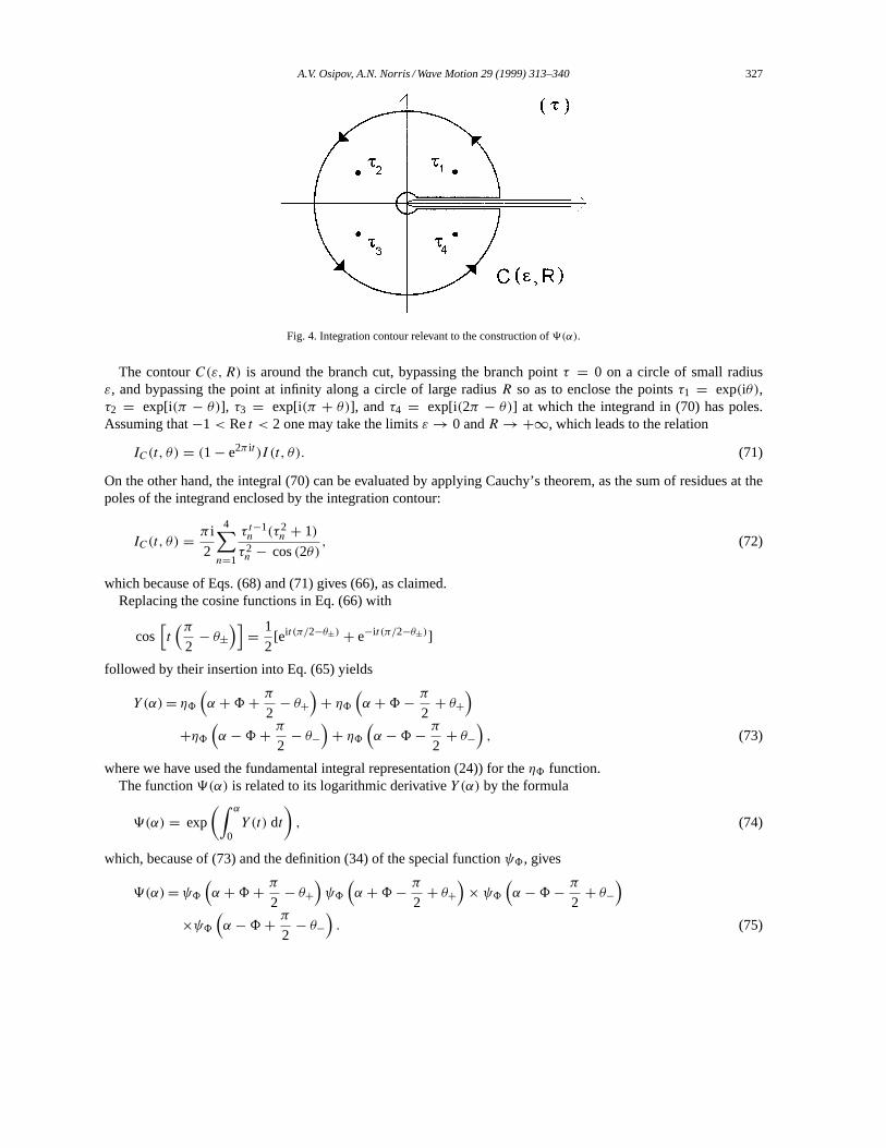
Fig. 4. Integration contour relevant to the construction of9(α).

The contourC(ε,R) is around the branch cut, bypassing the branch pointτ = 0 on a circle of small radiusε, and bypassing the point at infinity along a circle of large radiusR so as to enclose the pointsτ1 = exp(iθ),τ2 = exp[i(π − θ)], τ3 = exp[i(π + θ)], and τ4 = exp[i(2π − θ)] at which the integrand in (70) has poles.Assuming that−1< Ret < 2 one may take the limitsε → 0 andR → +∞, which leads to the relation

IC(t, θ) = (1 − e2π it )I (t, θ). (71)

On the other hand, the integral (70) can be evaluated by applying Cauchy’s theorem, as the sum of residues at thepoles of the integrand enclosed by the integration contour:

IC(t, θ) = π i

2

4∑n=1

τ t−1n (τ2

n + 1)

τ2n − cos(2θ)

, (72)

which because of Eqs. (68) and (71) gives (66), as claimed.Replacing the cosine functions in Eq. (66) with

cos[t(π

2− θ±

)]= 1

2[eit (π/2−θ±) + e−it (π/2−θ±)]

followed by their insertion into Eq. (65) yields

Y (α)= η8

(α +8+ π

2− θ+

)+ η8

(α +8− π

2+ θ+

)+η8

(α −8+ π

2− θ−

)+ η8

(α −8− π

2+ θ−

), (73)

where we have used the fundamental integral representation (24)) for theη8 function.The function9(α) is related to its logarithmic derivativeY (α) by the formula

9(α) = exp

(∫ α

0Y (t) dt

), (74)

which, because of (73) and the definition (34) of the special functionψ8, gives

9(α)=ψ8

(α +8+ π

2− θ+

)ψ8

(α +8− π

2+ θ+

)× ψ8

(α −8− π

2+ θ−

)×ψ8

(α −8+ π

2− θ−

). (75)


One may directly verify the validity of this formula by showing that it does satisfy the functional equations (58).Substituting9(α) from Eq. (75) directly into Eq. (58), and using the fact that the Malyuzhinets function is an evenfunction of its argument, leads to the relations

9(α ±8)

9(−α ±8)= ψ8(α ± 28+ π/2 − θ±)ψ8(α ± 28− π/2 + θ±)ψ8(α ∓ 28− π/2 + θ±)ψ8(α ∓ 28+ π/2 − θ±)

. (76)

These reduce to Eq. (58) by applying the functional property (36), thus verifying the fundamental identity (75).The poles and zeros of9(α) are simply those of the four Malyuzhinets functions appearing in Eq. (75). Corre-

spondingly, the poles of9(α) belong to the four families of points:

α = 8+ π + θ+ + 4n8,−38− π − θ+ − 4n8,−8− π − θ− − 4n8,38+ π + θ− + 4n8. (77)

with n = 0,1,2, . . . . Note that the absence of poles and zeros of9(α) in the strip50, which guarantees that thetransform functionS(α) given by Eq. (54) satisfies the regularity condition (53), is a consequence of the similaranalytic behaviour ofψ8(α) for |Reα| < 28+ 1

2π .The asymptotic behaviour of the function9(α) as Imα → ±∞ is given by

9(α) = 1

4ψ48

(π2

)e∓iνα[1 + o(1)], (78)

which results from (75) and the property (44). Eqs. (54) and (57), combined with the relation (78), ensure theboundedness of the spectral functionS(α) at the infinitely distant point Imα = ∞. This, along with the identity(5), specifies the finite value of the potential functionu(r, φ) at the edge of the wedge as

limr→0u(r, φ) = νU0ψ48

(π2

) cos(νφ0)

9(φ0). (79)

This completes the construction of the auxiliary function9(α) and, therefore, the proper transform functionS(α)relevant to diffraction from an impedance wedge, which is given by (54) together with (57) and (75). Beforeproceeding further it is useful to discuss some limiting cases.

Using the functional relation (37), one may rewrite Eq. (75) as follows

9(α)=ψ48

(π2

)cos

[ π48

(α +8− θ+)]

cos[ π

48(α −8+ θ−)

]

×ψ8(α +8− π2 + θ+)ψ8(α −8+ π

2 − θ−)ψ8(α +8− π

2 − θ+)ψ8(α −8+ π2 + θ−)

. (80)

Thus, when the wedge faces are identical, i.e.θ+ = θ−, the function9(α) is an even function of its argument.Furthermore, under certain circumstances,9(α) andS(α) may become 2π -periodic functions ofα. More pre-

cisely, this is the case for arbitrary face impedances if8 = π/(4m) with m integer, while for equal impedances ofthe faces the property holds when8 = π/(2q) andq = 1,2,3, . . . . All these particular cases relate to the case ofan interior wedge, and, as one may prove by a simple analysis of the Sommerfeld integral (2) assuming its integrandfunction to be 2π -periodic, the solution of the diffraction problemu(r, φ) can be then expressed without integration,through a finite number of residue contributions [15].

To prove the periodicity, first observe that the functionσ(α) is necessarily 2π -periodic when8 = π/(2q) withq an arbitrary integer, which results immediately from its representation (57). Next consider the auxiliary function9(α) given by (75) and notice the relation

9(α + 2π) = 9(α)

4∏k=1

cos [ π48(αk + 32π)]

cos [ π48(αk + 12π)]

(81)


with α1 = α + 8 − 12π + θ+, α2 = α + 8 + 1

2π − θ+, α3 = α − 8 − 12π + θ−, andα4 = α − 8 + 1

2π − θ−,which follows from repeated use of the functional property (37). The cosine functions in the numerator of Eq. (81)can be represented as

cos

[π

48

(αk + 3

2π

)]= cos

[π

48

(αk + 1

2π

)]cos

(π2

48

)− sin

[π

48

(αk + 1

2π

)]sin

(π2

48

),

which simplifies to(−1)m cos [ π48(αk + π2 )] when8 = π/(4m) withm integer. Thus, in the latter case the product

in Eq. (81) becomes unity, implying the 2π -periodicity of the9(α) function.If the impedances of the faces are the same, that is,θ+ = θ− = θ , this periodicity property of9(α) occurs for

the wider set of vertex angles given by8 = π/(2q)with q = 1,2,3, . . . , which for evenq reproduces the previouscase of arbitrary impedances. To make this clear, we rewrite the products of cosine functions from (81) as

4∏k=1

cos

[π

48

(αk + 1

2π

)]= 1

4cos

[ π28

(α + θ)]

cos[ π

28(π + α − θ)

],

4∏k=1

cos

[π

48

(αk + 3

2π

)]= 1

4cos

[ π28

(π + α + θ)]

cos[ π

28(2π + α − θ)

],

yielding

9(α + 2π) = 9(α)

2∏k=1

cos [ π28(βk + π)]

cos(πβk/(28))(82)

with β1 = α + θ andβ2 = α + π − θ . Again, one may readily check that the product in Eq. (82) is always unityif 8 = π/(2q) with integerq. Thus, we have established our claim concerning 2π -periodicity of the transformfunctionS(α).

Now consider what happens to the solution (54) in the particular cases of ideal boundaries. For vanishing valuesof the Brewster angles,|θ±| → 0, Eq. (80) reduces to

9(α) → 1

2ψ48

(π2

)cos

(πα28

), (83)

which, together with Eq. (54), yields

S(α) → U0ν cos(να)

sin(να)− sin(νφ0). (84)

Eq. (84) is a well-known expression for the transform function of a wedge with Neumann boundary conditions[1,2].

For a wedge with one face acoustically hard, say that atφ = −8, while the other face has finite, non-zeroimpedance, we get

S(α) = U0 σ(α)9(α)

9(φ0)

cos [ π48(α −8)]

cos [ π48(φ0 −8)], (85)

with

9(α) = ψ8

(α +8+ π

2− θ+

)ψ8

(α +8− π

2+ θ+

). (86)

The limit of Dirichlet boundary conditions, i.e. Im|θ±| → ∞, can be treated on the basis of the asymptotic estimate(44). This gives

|9(α)| → 1

4ψ48

(π2

)exp

[ π48

(|Im θ+| + |Im θ−|)]

(87)


for the9 function, and therefore, the quotient9(α)/9(φ0) in Eq. (54) tends to unity, yielding another well-knownlimiting expression

S(α) → U0ν cos(νφ0)

sin(να)− sin(νφ0), (88)

relevant to acoustically soft boundaries. If only one face of the wedge is acoustically soft, for instanceφ = −8,then taking the limit|Im θ−| → ∞ in Eq. (54) gives

S(α) = U09(α)

9(φ0)σ (α) (89)

with 9(α) defined in (86).We conclude this section by mentioning that the transformS(α) from Eq. (54) is clearly a meromorphic function

of the complex variableα. Its singularities are poles located at two subsets of points, one of which, given by Eq.(77), is related to the auxiliary function9(α), whereas the other subset comes from the trigonometric functionσ(α)

and these latter are as follows:

α = (−1)mφ0 + 2m8, m = 0,±1,±2, . . . (90)

Consequently, the transformS(α + φ) in Eq. (2) is analytic inside the loopsγ± as long as they do not enclose anypoles of the functions9(α + φ) andσ(α + φ). This is essentially the definition of the loops, which should residein the region where|Im α| > V with

V = sup(|Im θ±|, |Im φ0|). (91)

4. Near-field approximations

4.1. Series representation of the Malyuzhinets solution

The solution in Section 3 is in the form of a Sommerfeld integral (2) with its transform function given by Eq.(54). This is well suited to analysing the wave functionu(r, φ) far from the edge, wherekr � 1 and the saddle pointtechnique is applicable. On the other hand, this technique cannot be applied to evaluate the Sommerfeld integralin the near and intermediate zones wherekr ≤ 1. Another representation of the Malyuzhinets solution is thereforerequired to describe the wave field diffracted by an impedance wedge in the vicinity of its edge. In this section werepresent the Malyuzhinets solution as a series of Bessel functions [38], which in the limits of Dirichlet–Neumannboundary conditions reduces to the well-known expressions [1–7]

u(r, φ) = 4νU0

∞∑p=0

δpe−iνpπ/2Jνp (kr)χ [νp(8+ φ)]χ [νp(8+ φ0)], (92)

whereJνp (kr) are the Bessel functions of the first kind,ν = π/(28) is defined in (56), andδp = 1 if p ≥ 1. Thevalues of the other parametersδ0, νp as well as the definition ofχ(τ) depend upon the type of boundary conditions.They are as follows:δ0 = 1

2, νp = νp, andχ(τ) = cosτ if θ± = 0 (hard faces);δ0 = 1, νp = νp, andχ(τ) = sinτif Im θ± = ∞ (soft faces);δ0 = 1, νp = ν(p + 1

2), andχ(τ) = sinτ if θ+ = 0 and Imθ− = ∞ (mixed boundaryconditions).

We begin by noting that the Sommerfeld integral in (3) involves integration over one loopγ+ extending toIm α → +∞ and residing entirely in the upper half-plane Imα > 0. By referring to the analytical form of theexpansion of the trigonometrical factor in Eq. (54),

σ(±α + φ) = ∓ 2ν∞∑n=1

an−1(±φ0)exp[inν(α ± ϕ)+ in

π

2

], (93)


with an−1(φ0) = sin [n(νϕ0+π/2)], one may search for the expansion ofS(±α+φ) into a sequence of exponentialfunctions{ exp(iνpα)}+∞

p=0 such that 0≤ Reν0 < Reν1 < · · ·This is clearly achieved if the remaining factor in Eq. (54), that is,9(±α + φ) is expanded in a similar form. To

this end, it is useful to exploit series representations (42) from Section 2.3. Since Imα > V throughout the wholecontourγ+ we may replace all the Malyuzhinets functions occurring in (75) with the series representations (42),which yields

9(±α + φ) = 1

4ψ48

(π2

)e−iν(α±φ) exp

[ ∞∑k=1

b±k eiνk(α±φ) +

∞∑k=1

c±k ei(2k−1)(α±φ)], (94)

where

b±k = − cos [νk(π/2 − θ+)]

k cos(πνk/2)e∓iπk/2 − cos [νk(π/2 − θ−)]

k cos(πνk/2)e±iπk/2,

c±k = sin [(2k − 1)θ+]e±i(2k−1)8

(k − 12) sin [28(2k − 1)]

+ sin [(2k − 1)θ−]e∓i(2k−1)8

(k − 12) sin [28(2k − 1)]

.

(95)

The expansions (93) and (94) can now be used to rewrite the transform function as a double series

S(α) =+∞∑p,q=0

S±pqe±iνpqα, (96)

whereS±pq are constant coefficients andνpq = νp + q. Inserting Eq. (96) in Eq. (3) and using the integral repre-

sentation of the Bessel function

Jν(z) = − 1

2πeiνπ/2

∫γ+

e−iz cosα+iναdα, (97)

converts the Malyuzhinets solution into the series expression of the form

u(r, φ) = U0νψ4

8(π/2)

29(φ0)

∞∑p,q=0

Jνpq (kr)e−iνpqπ/2fp(φ0)(g

+q eipπ/2+iνpqφ + g−

q e−ipπ/2−iνpqφ). (98)

The coefficientsfp(φ0) andg±q may be obtained from the generating functions

∞∑q=0

g±q z

q = exp

( ∞∑k=1

c±k z2k−1

), (99)

∞∑p=0

fp(φ0)zp =

∞∑n=0

an(φ0)zn exp

( ∞∑k=1

bkzk

), (100)

wherebk = b−k e

iπk/2, while an(φ0), b−k , andc±k are defined in Eqs. (93) and (95), respectively.

By explicitly expanding the exponential functions in (99) and (100) into power series ofz, the rules (99) and(100) can be transformed into recurrent sequences convenient for numerical computations [38]. Specifically, thecoefficientsfp(φ0) are given by the relations

fp(φ0) =p∑k=0

ap−k(φ0) dk, (101)


where

d0 = 1, dk =k∑

m=1

1

m!d(m)k−m k ≥ 1,

and

d(j)

0 = bj

1, d(j)m = 1

mb1

m∑n=1

bn+1d(j)m−n(nj −m+ n).

The first three coefficients in Eq. (101) are as follows:f0(φ0) = a0(φ0), f1(φ0) = a1(φ0) + b1a0(φ0), andf2(φ0) = a2(φ0)+ b1a1(φ0)+ a0(φ0)(b2 + b2

1/2).The coefficientsg±

q with q = 1,2, . . . result from the successive use of the matrix recurrent relations

sin [28(q + 1)]GGGq+1 = KqGGGq + LqGGGq−1, (102)

with

Kq =(

ei8(2q+1) sinθ+ + e−i8(2q+1) sinθ− ei8 sinθ+ + e−i8 sinθ−e−i8 sinθ+ + ei8 sinθ− e−i8(2q+1) sinθ+ + ei8(2q+1) sinθ−

),

and

Lq =(

sin(2q8) − sin(28)− sin(28) sin(2q8)

).

HereGGGq = (g+q , g

−q )

T and the initial values for the recurrence procedure (102) areGGG−1 = (0,0)T andGGG0 = (1,1)T.

The first three coefficients are found from (102) as follows:g±0 = 1, g±

1 = c±1 , andg±2 = (c±1 )

2/2.In the limit asθ± → 0 the coefficientsg±

q andfp(φ0)becomeg±0 = 1 andg±

q = 0 withq ≥ 1 andf0(φ0) = a0(φ),f1(φ0) = a1(φ), andfp(φ0) = ap(φ) − ap−2(φ0) with p ≥ 2, respectively. This reduces the double series (98)to the single one (92) for the case of Neumann boundary conditions if the limiting expression (83) for the function9(φ0) is accounted for.

To consider the alternative case of the Dirichlet boundary conditions obtained in the limit|Im θ±| → ∞ weneed to return to the Sommerfeld integral (3) and take the limit with respect to the Brewster angles in the transformfunctionsS(±α+φ). If both faces of the wedge are acoustically soft, the limiting expression given by (88) involvesonly trigonometric functions and the corresponding Sommerfeld integral can be readily transformed into the Besselfunction series (92) (see, for example, [3]).

In order to obtain a series representation for the case of a wedge with one face acoustically soft and the other offinite impedance, one should start with the formula (89) and expand it into a sequence of exponential functions. Theexpansion is then inserted into (3) and the integral representation (97) for Bessel functions is again used, yieldingthe series

u(r, φ) = 2νU0ψ28(π/2)

9(φ0)

+∞∑p,q=0

Jνpq (kr)e−iνpqπ/2fp(φ0)gq sin [νpq(8+ φ)], (103)

whereνpq = ν(p + 12)+ q, and the function9(φ0) is defined by Eq. (87).

The coefficientsfp(φ0) andgq can be found by expanding the generating functions similar to those in Eqs. (99)and (100) with

bk = (−1)k+1 cos [νk(π/2 − θ+)]k cos(πνk/2)

, c+k = sin [(2k − 1)θ+]

(k − 12) sin [28(2k − 1)]

,


in place ofbk andc±k , respectively. The corresponding recurrence procedure forfp(φ0) results from Eq. (101) onreplacingbk with bk, whereas the one forgq is

gq+1 = 2 sinθ+cos(28q)

sin [28(q + 1)]gq + sin [28(q − 1)]

sin [28(q + 1)]gq−1, (104)

with g−1 = 0, g0 = 1, andq = 0,1,2, . . . One may check that in the limitθ+ → 0 the series (103) reduces to (92)for the case of mixed boundary conditions withθ+ = 0 and Imθ− = ∞.

The series (98) and (103) converge absolutely. This can be seen by noting that forn → ∞ the recurrence relations(101), (102) and (104) lead to the estimates

g±n = O(enV ), fn(φ0) = O(eνnV ), gn = O(en|Im θ+|), fn(φ0) = O(eνn|Im θ+|), (105)

with V defined in Eq. (91). Since for large and positiveν the Bessel functionsJν(kr) behave like O[(kr/ν)ν ], theestimates (105) guarantee the convergence of the series.

The members of (98) and (103) become negligible whenνpq > O(kreV ) andνpq > O(kre|Im θ+|), respectively.This means that the series representations are particularly useful for small and moderate values ofkr, since retaininga few leading terms in Eqs. (98) and (103) may provide accurate approximations for the whole series.

We may now consider the behaviour of the Malyuzhinets solution near the edge of the wedge, whenkr → 0.Replacing the Bessel functions in Eq. (98) with their ascending series

Jν(kr) =(kr

2

)ν ∞∑j=0

(−1)j

j !0(ν + j + 1)

(kr

2

)2j

, (106)

where0(α) is the Gamma function, transforms the solution into a power series of the form

u(r, φ) =∞∑p=0

(kr)νp∞∑m=0

Apm(φ)(kr)m, (107)

with coefficients directly related tog±q andfp(φ0). If kr is sufficiently small, we may retain only a few leading

terms in (107), yielding the approximation

u = A00 + A10(φ)(kr)ν + A01(φ)kr + O[(kr)2δ], (108)

whereδ = inf (ν,1) and

A00 = νU0ψ48(π/2)

9(φ0)cos(νφ0),

A01(φ) = −iνU0ψ48(π/2) cos(νφ0)

9(φ0) sin(28)[ sinθ+ cos(φ +8)+ sinθ− cos(φ −8)],

A10(φ) = U0νψ4

8(π/2) sin(νφ) cos(νφ0)

(2i)ν0(ν + 1)9(φ0)[2 sin(νφ0)− b1], (109)

with b1 = ib−1 defined from Eq. (95).

Eq. (108) describes the behaviour of the wave field near the edge of an impedance wedge.A00 is the main term.It characterises the value of the wave potentialu(r, φ) at the edge, and agrees with the limiting expression (79), asexpected. The next two terms of Eq. (108) are necessary to describe the edge behaviour of the derivatives∂u/∂r and∂u/(r∂φ) that represent the radial and angular components of the particle speed in the acoustic case or the associatedcomponents of the electric/magnetic fields in the electromagnetic case. If the wedge is acute, that is,8 > π/2, thenν < 1 and the first derivatives of the functionu(r, φ) with respect to any coordinate have a singularity of the form


A10(φ)(kr)ν−1 at the edge, which arises from the second term in Eq. (108). Alternatively, in the case of an internal

wedge, i.e.8 < π/2, the first derivatives are bounded at the edge and their behaviour depends on the third memberin the right part of Eq. (108), proportional toA01(φ).

The expansion (108) is also applicable if one or both faces of the wedge is acoustically hard, which can beconsidered by taking the appropriate limits with respect to the impedance parameters in equations (109). In the casethat one of the faces is acoustically soft, corresponding to the Dirichlet boundary condition, the formula (108) isreplaced by the following:

u(r, φ) = B00(φ)(kr)ν/2 + O[(kr)δ+ν/2], (110)

with

B00(φ) = U02νψ2

8(π/2) sin [ν(φ0 +8)]

(2i)ν/20(ν/2 + 1)9(φ0)sin

[ν2(8+ ϕ)

],

which follows from the relevant series representation (103).By contrast with Eq. (108), the expression (110) implies that irrespective of the wedge angle8 the wave potential

u(r, φ) vanishes askr → 0 while its first derivatives∂u/∂r and∂u/(r∂φ) tend to zero if8 < π/4 or are singularat the edge if8 > π/4, in accordance with the estimateu = O[(kr)−1+ν/2]. Notice that this singularity of the fieldderivatives is stronger than that for the wedge with faces acoustically hard or of non-zero impedance.

As it was pointed out in Section 2.3, certain terms in the expansion given by (42) and (43) may become infinitewhen8 = 8nm, where8nm = πn/[2(2m− 1)] with n andm integers. However, such singularities can be shownto cancel each other so that their sum (43) remains bounded, which means that these cases can be treated by simplytaking the limit8 → 8nm in the series expressions presented so far in this section. As a result of cancelling thesingularities the derivatives of the Bessel functionJν(kr) with respect toν may enter the series (98) and (103).Correspondingly, the logarithmic terms of the forms(kr)p ln q(kr) with integerp andq occur in the expansions(107). The analytic structure of the resulting series depends on the particular values ofm andn in8nm. Two specificexamples are presented next, forn,m = 1 (a flat surface with an impedance step), and forn = 2,m = 1 (animpedance half-plane).

Taking the limit8 → π/2 in Eq. (107) gives an expansion of the form

u(r, φ) =∞∑p=0

(kr)pp∑

m=0

Apm(φ) ln m(kr), (111)

which, for sufficiently small values ofkr, can be replaced by the formula

u(r, φ) = A00 + A11(φ)kr ln (kr)+ O(kr).

Here

A11(φ) = U0ψ48(π/2)

iπ9(φ0)( sinθ+ − sinθ−) cosφ0 sinφ,

while the coefficientA00 equalsA00 from Eq. (108) with8 = π/2. A consequence of Eq. (111) is that the firstderivatives∂u/∂r and∂u/(r∂φ) of the wave function for diffraction from an impedance step exhibit a logarithmicsingularity at the discontinuity point, rather than an algebraic power law singularity.

In the case of an impedance half-plane, one has the expansion

u(r, φ) =∞∑p=0

(kr)p∞∑m=0

ln m(kr)[A2p,m(φ)+ (kr)1/2A2p+1,m(φ)], (112)


with coefficients defined such thatAnm(φ) = 0 if n < m. Two leading terms of Eq. (112) are:

u(r, φ) = A00 +√krA10(φ)+ O(kr ln kr),

whereA00 = lim8→πA00 andA10(φ) = lim8→πA10(φ). Thus, at the edge of an impedance half-plane the singularcomponents of the wave field behave as O[(kr)−1/2].

Similar expansions occur if one face of the half-plane or the impedance step plane is acoustically soft. Theexpansions differ in their analytical form from (111) and (112) only by a factor(kr)ν/2, and the coefficients in theirleading terms are given byB00(φ) from Eq. (110) with8 → π/2 or8 → π , respectively.

4.2. The edge field

The value of the total field at the edge of an impedance wedge is not, in general, an easy quantity to computebecause of its dependence on Malyuzhinets functions. Although these are now well documented, and fast algorithmsexist for their computation (see Section 2.3), they are still cumbersome to handle as compared with trigonometricfunctions. In this section we show how the edge field can be described in a simple way, using only trigonometricfunctions. Also, the edge field is analysed as a function of the face impedances and the vertex angle of the wedge.

We will work with the normalised edge fieldu0(φ0) ≡ u(0, φ)/U0, which is the total field at the edge for a planewave of unit amplitude incident from directionφ0. It follows from the alternative form of9(α) in Eq. (80) that thelimiting expression (79) for the edge value of the total field can be rewritten

u0(φ) = ν cos(νφ)X+(φ, θ+)X−(φ, θ−)cos [ν2(φ +8− θ+)] cos [ν2(φ −8+ θ−)]

, (113)

where

X±(φ, θ) = ψ8[φ ± (8− π/2 − θ)]

ψ8[φ ± (8− π/2 + θ)]. (114)

If the impedance of a face is a pure reactance, that is, it is purely imaginary, then the associated angle,θ+ orθ−, is also purely imaginary. Let us assume for the moment that this is the case for both faces, then the fact thatψ8(α) = ψ8(α) implies that|X±(φ, θ±)| = 1. The denominator in Eq. (113) can be further simplified by splittingthe terms sin [ν(φ − θ+)] and sin [ν(φ + θ−)] into their real and imaginary parts, yielding

|u0(φ)| = 2ν cos(νφ)

[ cosh(ν|θ+|)− sin(νφ)]1/2[ cosh(ν|θ−|)+ sin(νφ)]1/2. (115)

Thus, in general

|u0(φ)| ≤ π

8for reactive faces, (116)

with equality for the rigid wedge(θ+ = θ− = 0).The upper bound (116) may be replaced by an exponential bound in certain cases. For example, the identity (115)

implies that the total field at the vertex of a narrow wedge-shaped region with reactive faces such thatν|θ±| � 1 isexponentially small, and less than 4ν exp[− ν

2(|θ+| + |θ−|)] in magnitude.Pierce and Hadden [52] considered diffraction from a wedge with finite but large impedance, in which case

approximations can be made using the rigid limit as reference. The same can be achieved for the tip field as follows.For hard faces the anglesθ± are small. For simplicity, we consider the case of identical impedances,θ± = θ , andfind after a simple expansion of (113) that

u0(φ) ≈ π

8

[1 − θν

cos(νφ)+ 2θη8

(φ −8+ π

2

)− 2θη8

(φ +8− π

2

)]. (117)


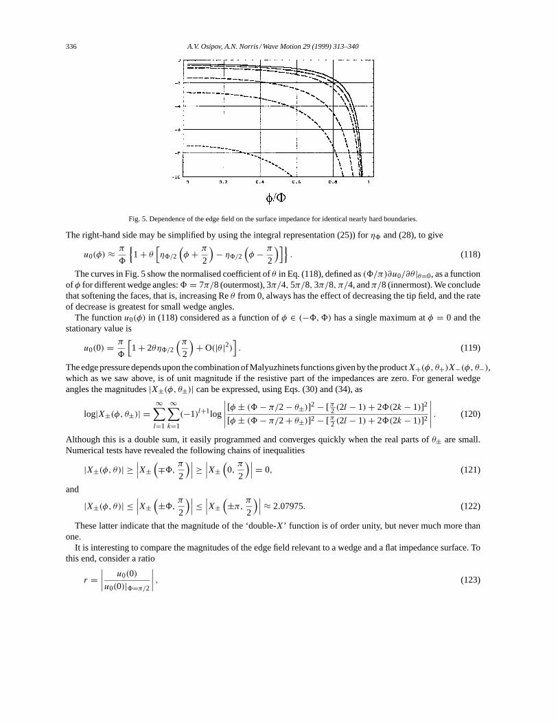
Fig. 5. Dependence of the edge field on the surface impedance for identical nearly hard boundaries.

The right-hand side may be simplified by using the integral representation (25)) forη8 and (28), to give

u0(φ) ≈ π

8

{1 + θ

[η8/2

(φ + π

2

)− η8/2

(φ − π

2

)]}. (118)

The curves in Fig. 5 show the normalised coefficient ofθ in Eq. (118), defined as(8/π)∂u0/∂θ |θ=0, as a functionof φ for different wedge angles:8 = 7π/8 (outermost), 3π/4,5π/8,3π/8, π/4, andπ/8 (innermost). We concludethat softening the faces, that is, increasing Reθ from 0, always has the effect of decreasing the tip field, and the rateof decrease is greatest for small wedge angles.

The functionu0(φ) in (118) considered as a function ofφ ∈ (−8,8) has a single maximum atφ = 0 and thestationary value is

u0(0) = π

8

[1 + 2θη8/2

(π2

)+ O(|θ |2)

]. (119)

The edge pressure depends upon the combination of Malyuzhinets functions given by the productX+(φ, θ+)X−(φ, θ−),which as we saw above, is of unit magnitude if the resistive part of the impedances are zero. For general wedgeangles the magnitudes|X±(φ, θ±)| can be expressed, using Eqs. (30) and (34), as

log|X±(φ, θ±)| =∞∑l=1

∞∑k=1

(−1)l+1log

∣∣∣∣∣ [φ ± (8− π/2 − θ±)]2 − [ π2 (2l − 1)+ 28(2k − 1)]2

[φ ± (8− π/2 + θ±)]2 − [ π2 (2l − 1)+ 28(2k − 1)]2

∣∣∣∣∣ . (120)

Although this is a double sum, it easily programmed and converges quickly when the real parts ofθ± are small.Numerical tests have revealed the following chains of inequalities

|X±(φ, θ)| ≥∣∣∣X±

(∓8, π

2

)∣∣∣ ≥∣∣∣X±

(0,π

2

)∣∣∣ = 0, (121)

and

|X±(φ, θ)| ≤∣∣∣X±

(±8, π

2

)∣∣∣ ≤∣∣∣X±

(±π, π

2

)∣∣∣ ≈ 2.07975. (122)

These latter indicate that the magnitude of the ‘double-X’ function is of order unity, but never much more thanone.

It is interesting to compare the magnitudes of the edge field relevant to a wedge and a flat impedance surface. Tothis end, consider a ratio

r =∣∣∣∣ u0(0)

u0(0)|8=π/2

∣∣∣∣ , (123)


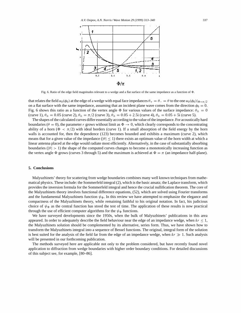
Fig. 6. Ratio of the edge field magnitudes relevant to a wedge and a flat surface of the same impedance as a function of8.

that relates the fieldu0(φ0) at the edge of a wedge with equal face impedancesθ+ = θ− = θ to the oneu0(φ0)|8=π/2on a flat surface with the same impedance, assuming that an incident plane wave comes from the directionφ0 = 0.Fig. 6 shows this ratio as a function of the vertex angle8 for various values of the surface impedance:θ± = 0(curve 1),θ± = 0.05 (curve 2),θ± = π/2 (curve 3),θ± = 0.05+ 2.5i (curve 4),θ± = 0.05+ 5i (curve 5).

The shapes of the calculated curves differ essentially according to the value of the impedance. For acoustically hardboundaries (θ = 0), the parameterr grows without limit as8 → 0, which clearly corresponds to the concentratingability of a horn (8 < π/2) with ideal borders (curve 1). If a small absorption of the field energy by the hornwalls is accounted for, then the dependence (123) becomes bounded and exhibits a maximum (curve 2), whichmeans that for a given value of the impedance (|θ | ≤ 1) there exists an optimum value of the horn width at which alinear antenna placed at the edge would radiate most efficiently. Alternatively, in the case of substantially absorbingboundaries (|θ | > 1) the shape of the computed curves changes to become a monotonically increasing function asthe vertex angle8 grows (curves 3 through 5) and the maximum is achieved at8 = π (an impedance half-plane).

5. Conclusions

Malyuzhinets’ theory for scattering from wedge boundaries combines many well known techniques from mathe-matical physics. These include: the Sommerfeld integral (2), which is the basic ansatz; the Laplace transform, whichprovides the inversion formula for the Sommerfeld integral and hence the crucial nullification theorem. The core ofthe Malyuzhinets theory involves functional difference equations, (52), which are solved using Fourier transformsand the fundamental Malyuzhinets functionψ8. In this review we have attempted to emphasize the elegance andcompactness of the Malyuzhinets theory, while remaining faithful to his original notation. In fact, his judiciouschoice ofψ8 as the central function has stood the test of time. The application of these results is now practicalthrough the use of efficient computer algorithms for theψ8 functions.

We have surveyed developments since the 1950s, when the bulk of Malyuzhinets’ publications in this areaappeared. In order to adequately describe the field behaviour near the edge of an impedance wedge, whenkr ≤ 1,the Malyuzhinets solution should be complemented by its alternative, series form. Thus, we have shown how totransform the Malyuzhinets integral into a sequence of Bessel functions. The original, integral form of the solutionis best suited for the analysis of the field far from the edge of an impedance wedge, whenkr � 1. Such analysiswill be presented in our forthcoming publication.

The methods surveyed here are applicable not only to the problem considered, but have recently found novelapplication to diffraction from wedge boundaries with higher order boundary conditions. For detailed discussionsof this subject see, for example, [80–86].


This paper has dealt with two dimensional fields applicable to the case when the incident wave falls at a rightangle to the edge of the wedge, and consequently there is no dependence upon the third coordinate, sayz, measuredalong the edge. A three dimensional extension of the Malyuzhinets solution for scattering of an obliquely incidentplane wave from an impedance wedge is quite straightforward in acoustics. It can be achieved by separating out thisdependence in the exponential factor exp(−ikz sinχ0) whereχ0 is the skewness angle andχ0 = 0 corresponds tonormal incidence.

In contrast, the case of oblique or skew incidence in electromagnetics implies qualitative complications becauseof a need to work with vector Maxwell’s equations rather than with a scalar Helmholtz equation. Generally, onehas to solve a system of coupled equations for two unknown spectral functions and the solutions reported in theliterature so far relate only to particular cases which are a wedge with surface impedance unity (θ± = π/2), a fullplane impedance junction (8 = π/2), a half plane (8 = π ), and right-angled exterior (8 = 3π/4) and interior(8 = π/4) wedges. The interested reader is referred to [73,87] for recent references and further discussion of thissubject.

Similar complications arise for the elastic problem, in which the region−8 < φ < 8 is described by theequations of isotropic dynamic elasticity, and the faces are either rigidly clamped or free of traction. The presentanalysis applies to the case of a shear wave polarised in the out-of-plane orz-direction. Any other polarization orany skew incidence of the shear wave leads to mode coupling and the problem once again becomes vectorial innature, such that it can not be solved any more in an explicit form (see, for example, [66]).

Acknowledgements

The work of A.N. Norris was supported by the Office of Naval Research.

References

[1] J.J. Bowman, T.B.A. Senior, The Wedge, in: J.J. Bowman, T.B.A. Senior, P.L.E. Uslenghi (Eds.), Electromagnetic and Acoustic Scatteringby Simple Shapes, North-Holland, Amsterdam, 1969, pp. 252–283.

[2] A.D. Pierce, Acoustics: An Introduction to its Physical Principles and Applications, Acoustical Society of America, Woodbury, NY, 1989.[3] G.I. Petrashen’, B.G. Nikolaev, D.P. Kouzov, On the method of series in the theory of diffraction of waves from flat angular regions,

Leningrad State University Scientific Reports: Math. Sci. 246 (1958) 5–165 (in Russian).[4] F. Oberhettinger, On the diffraction and reflection of waves and pulses by wedges and corners, J. Res. NBS 61 (1958) 343–365.[5] A.A. Tuzhilin, New representations of diffraction fields in wedge-shaped regions with ideal boundaries, Sov. Phys. Acoust. 9 (1963)

168–172.[6] P. Ambaud, A. Bergassoli, The problem of the wedge in acoustics, Acustica 27 (1972) 291–298.[7] L.B. Felsen, N. Marcuvitz, Radiation and Scattering of Waves, Prentice Hall, New York, 1978.[8] W.J. Hadden, Jr., A.D. Pierce, Sound diffraction around screens and wedges for arbitrary point source locations, J. Acoust. Soc. Am. 69

(1981) 1266–1276. Erratum: J. Acoust. Soc. Am. 71 (1982) 1290.[9] C. DeWitt-Morette, S.G. Low, L.S. Schulman, A.Y. Shiekh, Wedges I, Foundations of Physics 16 (1986) 311–349.

[10] G.D. Malyuzhinets, Generalisation of the Reflection Method in the Theory of Diffraction of Sinusoidal Waves, Doctoral dissertation, P.N.Lebedev Phys. Inst. Acad. Sci. USSR, 1950 (in Russian).

[11] G.D. Malyuzhinets, The radiation of sound by the vibrating boundaries of an arbitrary wedge. Part I, Sov. Phys. Acoust. 1 (1955) 152–174.[12] G.D. Malyuzhinets, Radiation of sound from the vibrating faces of an arbitrary wedge Part II, Sov. Phys. Acoust. 1 (1955) 240–248.[13] G.D. Malyuzhinets, Inversion formula for the Sommerfeld integral, Sov. Phys. Dokl. 3 (1958) 52–56.[14] G.D. Malyuzhinets, Relation between the inversion formulas for the Sommerfeld integral and the formulas of Kontorovich–Lebedev, Sov.

Phys. Dokl. 3 (1958) 266–268.[15] G.D. Malyuzhinets, Excitation, reflection and emission of surface waves from a wedge with given face impedances, Sov. Phys. Dokl. 3

(1958) 752–755.[16] G.D. Malyuzhinets, Das Sommerfeldsche Integral und die Losung von Beugungsaufgaben in Winkelgebieten, Ann. Phys. 6 (1960) 107–112,

in German.[17] W.E. Williams, Diffraction of an E-polarised plane wave by an imperfectly conducting wedge, Proc. R. Soc. London A 252 (1959) 376–393.[18] T.B.A. Senior, Diffraction by an imperfectly conducting wedge, Comm. Pure Appl. Math. 12 (1959) 337–372.


[19] A.A. Tuzhilin, Theory of Malyuzhinets’ functional equations. I. Homogeneous functional equations, general properties of their solutions,particular cases, Differents. Uravnenija 6 (1970) 692–704 (in Russian).

[20] A.A. Tuzhilin, Theory of Malyuzhinets’ functional equations. II. The theory of Barnes’ infinite products. General solutions of homogeneousMalyuzhinets’ functional equations. Various representations of the basis solutions, Differents. Uravnenija 6 (1970) 1048–1063 (in Russian).

[21] A.A. Tuzhilin, Theory of Malyuzhinets’ functional equations. III. Non-homogeneous functional equations. The general theory, Differents.Uravnenija 7 (1971) 1077–1088 (in Russian).

[22] A.A. Tuzhilin, Diffraction of a plane sound wave in an angular region with absolutely hard and slippery faces covered by thin elastic plates,Differents. Uravnenija 9 (1973) 1875–1888 (in Russian).

[23] G.D. Malyuzhinets, An accurate solution to a problem of diffraction of a plane wave by a semi-infinite elastic plate, Proc. 4th All-UnionAcoustics Conf., vol. 45, Academy of Science, Moscow, USSR, 1958 (in Russian).

[24] G.D. Malyuzhinets, A.A. Tuzhilin, Diffraction of a plane sound wave by a thin semi-infinite elastic plate, Zh. Vych. Matem. i Matem. Fiz.10 (1970) 1210–1227 (in Russian).

[25] G.D. Malyuzhinets, Sound diffraction and the surface waves propagating over a semi-infinite elastic plate, Trudy Akust. Inst. 15 (1971)80–96 (in Russian).

[26] M.P. Sakharova, A.F. Filippov, Solution of a nonstationary problem of diffraction by an impedance wedge in tabulated functions, Zh. Vych.Matem. i Mat. Fiziki 7 (1967) 568–579 (in Russian).

[27] A.F. Filippov, Investigation of solution of a nonstationary problem of diffraction of a plane wave by an impedance wedge, Zh. Vych. Matem.i Mat. Fiziki 7 (1967) 825–835 (in Russian).

[28] V.Yu. Zavadskii, M.P. Sakharova, Tables of the Special Functionψ8(z), Akust. Inst. Rep., Moscow, 1961.[29] V.Yu. Zavadskii, M.P. Sakharova, Application of the special functionψ8 in problems of wave diffraction in wedge-shaped regions, Sov.

Phys. Acoust. 13 (1967) 48–54.[30] M.P. Sakharova, On asymptotic expansion of certain functions occurring in the wedge diffraction theory, Izv. Vuzov. Fizika (11) (1970)

141–144 (in Russian).[31] J.L. Volakis, T.B.A. Senior, Simple expressions for a function occurring in diffraction theory, IEEE Trans. Antennas Propagat. 33 (1985)

678–680.[32] K. Hongo, E. Nakajima, Polynomial approximation of Malyuzhinets’ function, IEEE Trans. Antennas Propagat. 34 (1986) 942–947.[33] M.I. Herman, J.L. Volakis, T.B.A. Senior, Analytic expressions for a function occurring in diffraction theory, IEEE Trans. Antennas

Propagat. 35 (1987) 1083–1086.[34] A.V. Osipov, Calculation of the Malyuzhinets function in a complex region, Sov. Phys. Acoust. 36 (1990) 63–66.[35] M. Aidi, J. Lavergnat, Approximation of the Maliuzhinets function, Journal of Electromagnetic Waves and Applications 10 (1996) 1395–

1411.[36] Hu Jin-Lin, Lin Shi-Ming, Wang Wen-Bing, Calculation of Maliuzhinets function in complex region, IEEE Trans. Antennas Propagat. 44

(1996) 1195–1196.[37] B.V. Budaev, G.I. Petrashen’, On efficient approaches to solving the problem of wave diffraction from wedge-shaped regions, in: Problems

of the Dynamic Theory of Seismic Wave Propagation, Steklov Mathematical Institute, Leningrad, vol. 23, 1983, pp. 78–91 (in Russian).[38] A.V. Osipov, Diffraction of a plane wave in a corner region with impedance boundary conditions, Sov. Phys. Acoust. 37 (1991) 381–385.[39] J.J. Bowman, High-frequency scattering from an absorbing infinite strip with arbitrary face impedance, Can. J. Phys. 45 (1967) 2409–2430.[40] O.M. Bucci, G. Franceschetti, Electromagnetic scattering by a half-plane plane with two face impedances, Radio Sci. 11 (1976) 49–59.[41] S.N. Karp, F.C. Karal, A new method for the determination of the far-fields with applications to the problem of radiation of a line source

at the tip of an absorbing wedge, IEEE Trans. Antennas Propagat. 7 (1959) S91-S102.[42] W.E. Williams, Propagation of electromagnetic surface waves along wedge surfaces, Quart. J. Mech. Appl. Math. 13 (1960) 278–284.[43] W.E. Williams, Vertex generated waves outside metallic wedges, Proc. Cambridge Phil. Soc. 57 (1961) 393–400.[44] R.P. Starovoitova, M.S. Bobrovnikov, Excitation of an impedance wedge by a line magnetic current placed at the vertex, Izv. Vuzov. Fizika

(4) (1962) 130–139 (in Russian).[45] M.S. Bobrovnikov, V.V. Fisanov, Diffraction of Waves in Sector Regions, Tomsk State University, Tomsk, Russia, 1988 (in Russian).[46] G. Pelosi, R. Tiberio, R.G. Rojas, Electromagnetic field excited by a line source placed at the edge of an impedance wedge, IEEE Trans.

Antennas Propagat. 39 (1991) 1043–1046.[47] M.F. Otero, R.G. Rojas, Two-dimensional Green’s function for a wedge with impedance faces, IEEE Trans. Antennas Propagat. 45 (1997)

1799–1809.[48] A. Osipov, K. Hongo, The Green function of an impedance wedge, Electromagnetics 18 (1998) 135–167.[49] M.P. Zavadskaya, R.P. Starovoitova, Edge waves in G.D. Malyuzhinets’ solution for an impedance wedge, Sov. Phys. Acoust. 34 (1988)

678–680.[50] R.P. Starovoitova, M.S. Bobrovnikov, V.N. Kislicyna, Diffraction of a surface wave by an edge in an impedance plane, Radiotekh. Elektron.

7 (1962) 250–259 (in Russian).[51] M.S. Bobrovnikov, V.N. Ponomareva, V.G. Myshkin, R.P. Starovoitova, Diffraction of a skewly incident surface wave by an edge in an

impedance surface, Izv. Vuzov. Fizika 1 (1965) 162–169 (in Russian).[52] A.D. Pierce, W.J. Hadden Jr., Plane wave diffraction by a wedge with finite impedance, J. Acoust. Soc. Am. 63 (1978) 17–27.[53] T. Griesser, C.A. Balanis, Reflections, diffractions, and surface waves for an interior impedance wedge of arbitrary angle, IEEE Trans.

Antennas Propagat. 37 (1989) 927–935.


[54] A.V. Osipov, Uniform asymptotic formula for calculating an acoustic field near a face of an impedance wedge, Sov. Phys. Acoust. 36 (1990)180–183.

[55] A.V. Osipov, Asymptotic representation of the sound field in a narrow angular region with impedance boundaries, Sov. Phys. Acoust. 36(1990) 287–290.

[56] A.V. Osipov, On radar invisibility of an impedance wedge, IEEE AP-S Int. Symposium and URSI North American Radio Science Meeting,Montreal, Quebec, Canada, 13–18 July 1997, URSI Digest, p. 724.

[57] G.L. James, Uniform diffraction coefficients for an impedance wedge, Electron. Lett. 13 (1977) 403–404.[58] R. Tiberio, G. Pelosi, G. Manara, A uniform GTD formulation for the diffraction by a wedge with impedance faces, IEEE Trans. Antennas

Propagat. 33 (1985) 867–873.[59] G. Pelosi, S. Maci, R. Tiberio, A. Michaeli, Incremental length diffraction coefficients for an impedance wedge, IEEE Trans. Antennas

Propagat. 40 (1992) 1201–1210.[60] M.S. Bobrovnikov, R.P. Starovoitova, Diffraction of cylindrical waves by an impedance wedge, Izv. Vuzov. Fizika (6) (1963) 168–176 (in

Russian).[61] R. Tiberio, G. Pelosi, G. Manara, P.H. Pathak, High-frequency c scattering from a wedge with impedance faces illuminated by a line source,

Part I: Diffraction, IEEE Trans. Antennas Propagat. 37 (1989) 212–218.[62] V.F. Kravchenko, V.M. Likhachev, A.I. Stashkevich, On one asymptotic method of solution of a boundary-value problem for impedance

wedge excitation, Dokl. Akad. Nauk USSR 308 (1989) 329–334 (in Russian).[63] V.M. Likhachev, A.I. Stashkevich, Diffraction of a cylindrical wave in an impedance angular region, Radiotekh. Electron. 35 (1990) 707–717

(in Russian).[64] G. Manara, R. Tiberio, G. Pelosi, High-frequency scattering from a wedge with impedance faces illuminated by a line source, Part II:

Surface waves, IEEE Trans. Antennas Propagat. 41 (1993) 877–883.[65] N.N. Lebedev, I.P. Skal’skaja, A new method for solving the problems of diffraction of electromagnetic waves by a wedge of finite

conductivity, Sov. Phys. Tech. Phys. 4 (1962) 627–637.[66] B. Budaev, Diffraction by Wedges, Longman Scientific and Technical, UK, 1995.[67] B. Noble, Methods Based on the Wiener–Hopf Technique, Pergamon Press, London, 1958.[68] F.C. Karal, S.N. Karp, Diffraction of a skew plane electromagnetic wave by an absorbing right angled wedge, Comm. Pure Appl. Math. 11

(1958) 495–533.[69] F.C. Karal, S.N. Karp, R.G. Kouyoumjian, Scattering of a surface wave by a discontinuity in the surface reactance on a right-angled wedge,

Comm. Pure Appl. Math. 14 (1961) 35–48.[70] W.E. Williams, Diffraction by an imperfectly conducting wedge, Proc. Cambr. Phil. Soc. 55 (1959) 195–209.[71] W.E. Williams, A note on the diffraction by a right-angled wedge, Proc. Cambr. Phil. Soc. 61 (1965) 275–278.[72] T.B.A. Senior, Some problems involving imperfect half plane, in: P.L.E. Uslenghi (Ed.), Electromagnetic Scattering, Academic Press, New

York, 1978.[73] T.B.A. Senior, J.L. Volakis, Approximate Boundary Conditions in Electromagnetics, IEE Press, Stevenage, UK, 1995.[74] A.N. Norris, G.R. Wickham, Acoustic diffraction from the junction of two flat plates, Proc. R. Soc. Lond. A 451 (1995) 631–656.[75] A.G.R. Van Lennep, The kernel of Sommerfeld’s transform as solution to difference equations for a class of diffraction problems, J. Appl.

Phys. 45 (1974) 4401–4405.[76] A.V. Osipov, Malyuzhinets transform and the method of Sommerfeld integral in the theory of diffraction of waves in wedge-shaped domains,

in: Problems of Diffraction and Wave Propagation, St. Petersburg State University, St. Petersburg, Russia, vol. 25, 1993, pp. 148–173.[77] A.N. Norris, A.V. Osipov, Far-field analysis of the Malyuzhinets solution for plane and surface waves diffraction by an impedance wedge,

Wave Motion (1998), accepted.[78] F.W.J. Olver, Asymptotics and Special Functions, Academic Press, New York, 1974.[79] R. Mittra, S.W. Lee, Analytical Techniques in the Theory of Guided Waves, Macmillan, New York, 1974.[80] A.V. Osipov, General solution for a class of diffraction problems, J. Phys. A: Math. Gen. 27 (1994) L27–L32.[81] I.D. Abrahams, J.B. Lawrie, Travelling waves on a membrane: reflection and transmission at a corner of arbitrary angle I., Proc. Roy. Soc.

Lond. A 451 (1995) 657–683.[82] J.B. Lawrie, I.D. Abrahams, Travelling waves on a membrane: reflection and transmission at a corner of arbitrary angle. II., Proc. Roy. Soc.

Lond. A 452 (1996) 1649–1677.[83] A.V. Osipov, Diffraction by a wedge with higher-order boundary conditions, Radio Sci. 31 (1996) 1705–1720.[84] M.A. Ljalinov, Diffraction of a plane wave by a wedge with thin material coatings, Radio Sci. 31 (1996) 1721–1730.[85] A.V. Osipov, A.N. Norris, Acoustic diffraction by a fluid-loaded membrane corner, Proc. Roy. Soc. Lond. A 453 (1997) 43–64.[86] A.N. Norris, A.V. Osipov, Structural and acoustical wave interaction at a wedge-shaped junction of fluid loaded plates, J. Acoust. Soc. Am.

101 (1997) 867–876.[87] C.C. Constantinou, C. Demetrescu, A.V. Osipov, Diffraction by an impedance wedge at oblique incidence, Proc. 1998 URSI Int. Symp. on

Electromagnetic Theory, 25–27 May 1998, Thessaloniki, Greece, pp. 402–404.

Documents

The Malyuzhinets theory for scattering from wedge ...norris/papers/1999... · Wave Motion 29 (1999) 313–340 The Malyuzhinets theory for scattering from wedge boundaries: a review