Embed Size (px)
Citation preview

COMPUTER SCIENCE REPORTS
Report 02-12
March 2012
THE MANUAL FOR COLORED PETRI NETS IN SNOOPY – QPNC/SPNC/CPNC/GHPNC
FEI LIU MONIKA HEINER
CHRISTIAN ROHR
Faculty of Mathematics, Natural Sciences and Computer Science
Institute of Computer Science

Computer Science Reports Brandenburg University of Technology Cottbus ISSN: 1437-7969 Send requests to: BTU Cottbus Institut für Informatik Postfach 10 13 44 D-03013 Cottbus

Computer Science Reports 02-12
March 2012
Brandenburg University of Technology Cottbus
Faculty of Mathematics, Natural Sciences and Computer Science
Institute of Computer Science
Fei Liu, Monika Heiner, Christian Rohr [email protected], [email protected],
[email protected] www-dssz.informatik.tu-cottbus.de
The Manual for Colored Petri Nets in Snoopy – QPNC/SPNC/CPNC/GHPNC

Computer Science Reports Brandenburg University of Technology Cottbus Institute of Computer Science Head of Institute: Prof. Dr. Hartmut König [email protected] BTU Cottbus Institut für Informatik Postfach 10 13 44 D-03013 Cottbus Research Groups: Headed by: Computer Engineering Prof. Dr. H. Th. Vierhaus Computer Network and Communication Systems Prof. Dr. H. König Data Structures and Software Dependability Prof. Dr. M. Heiner Database and Information Systems Prof. Dr. I. Schmitt Programming Languages and Compiler Construction Prof. Dr. P. Hofstedt Software and Systems Engineering Prof. Dr. C. Lewerentz Theoretical Computer Science Prof. Dr. K. Meer Graphics Systems PD Dr. D. Cunningham Systems Prof. Dr. R. Kraemer Distributed Systems and Operating Systems Prof. Dr. J. Nolte Internet-Technology Prof. Dr. G. Wagner CR Subject Classification (1998): I.6.5, I.6.8, D.2.2, J.3 Printing and Binding: BTU Cottbus ISSN: 1437-7969

The Manual for Colored Petri Nets in Snoopy
— QPN C/SPN C/CPN C/GHPN C
Fei Liu, Monika Heiner and Christian Rohr
– Data Structures and Software Dependability –Institute of Computer Science
Brandenburg University of TechnologyCottbus, Germany
Abstract
Colored Petri nets are an excellent formalism for modeling and analyzing complex sys-tems. In Snoopy, we have implemented functionalities for editing, and animating/simu-lating colored qualitative Petri nets (QPN C), colored stochastic Petri nets (SPN C), col-ored continuous Petri nets (CPN C), and colored generalized hybrid Petri nets (GHPN C).In this manual, we demonstrate how to construct colored Petri nets step by step usinga simple example and describe some key modeling problems, e.g. automatic coloringPetri nets, specifying initial markings, or specifying rate functions. We also give ourannotation language and describe how to use this language to declare or define inscrip-tions of colored Petri nets, e.g. color sets, arc expressions or guards. In addition, wedescribe the animation, simulation, and analysis of colored Petri nets and show possibleimport/export relationships among different net classes. Finally, we give some examplesto demonstrate the application of colored Petri nets. In summary, this manual contains anumber of relevant materials for understanding, constructing, simulating and analyzingcolored Petri nets so that the user will have no difficulties in using colored Petri nets.
∗Please sent all questions, comments and suggestions how to improve this material to this address.
5

Liu, Heiner, Rohr
Contents
1 Introduction 91.1 Colored Petri nets . . . . . . . . . . . . . . . . . . . . . . . . . . . . . . . 9
1.2 Some notes . . . . . . . . . . . . . . . . . . . . . . . . . . . . . . . . . . . 111.3 Features - overview . . . . . . . . . . . . . . . . . . . . . . . . . . . . . . 11
1.3.1 Features for modeling . . . . . . . . . . . . . . . . . . . . . . . . . 111.3.2 Features for animation (for QPN C/SPN C) . . . . . . . . . . . . . 12
1.3.3 Features for simulation (for SPN C/CPN C/GHPN C) . . . . . . . . 121.3.4 Other features . . . . . . . . . . . . . . . . . . . . . . . . . . . . . 12
2 Modeling 142.1 General modeling procedure - an introductory example . . . . . . . . . . . 14
2.1.1 Transform a standard Petri net into a colored Petri net . . . . . . 142.1.2 Define similar subnets in the Petri net . . . . . . . . . . . . . . . . 15
2.1.3 Define declarations . . . . . . . . . . . . . . . . . . . . . . . . . . 152.1.4 Assign color sets to places and define initial markings . . . . . . . 17
2.1.5 Define arc expressions . . . . . . . . . . . . . . . . . . . . . . . . . 192.1.6 Define guards for transitions . . . . . . . . . . . . . . . . . . . . . 19
2.1.7 Define rate functions for transitions (for SPN C/CPN C/GHPN C) . 202.2 Constructing colored Petri nets . . . . . . . . . . . . . . . . . . . . . . . . 22
2.2.1 Basic colored Petri net components . . . . . . . . . . . . . . . . . . 222.2.2 Modeling branch and conflict reactions . . . . . . . . . . . . . . . . 23
2.2.3 Modeling nets with logical nodes . . . . . . . . . . . . . . . . . . . 242.3 Automatic colorizing . . . . . . . . . . . . . . . . . . . . . . . . . . . . . . 24
2.3.1 Colorizing any subset . . . . . . . . . . . . . . . . . . . . . . . . . 272.3.2 Colorizing twin nets . . . . . . . . . . . . . . . . . . . . . . . . . . 27
2.3.3 Colorizing T-invariants . . . . . . . . . . . . . . . . . . . . . . . . . 272.4 Some other key modeling problems . . . . . . . . . . . . . . . . . . . . . 27
2.4.1 Specifying initial markings . . . . . . . . . . . . . . . . . . . . . . 27
2.4.2 Random generation of initial marking (for SPN C) . . . . . . . . . 28
2.4.3 Specifying rate functions . . . . . . . . . . . . . . . . . . . . . . . . 292.4.4 Extended arc types . . . . . . . . . . . . . . . . . . . . . . . . . . . 30
2.4.5 Definition of auxiliary variables (observers) . . . . . . . . . . . . . 322.4.6 Consistency checks . . . . . . . . . . . . . . . . . . . . . . . . . . . 33
3 Annotation Language 34
3.1 Declarations . . . . . . . . . . . . . . . . . . . . . . . . . . . . . . . . . . 34
3.1.1 Color sets . . . . . . . . . . . . . . . . . . . . . . . . . . . . . . . 34
3.1.2 Subsets of color sets . . . . . . . . . . . . . . . . . . . . . . . . . . 37
3.1.3 Variables . . . . . . . . . . . . . . . . . . . . . . . . . . . . . . . . 373.1.4 Constants . . . . . . . . . . . . . . . . . . . . . . . . . . . . . . . 38
3.1.5 Functions . . . . . . . . . . . . . . . . . . . . . . . . . . . . . . . . 383.2 Expressions . . . . . . . . . . . . . . . . . . . . . . . . . . . . . . . . . . . 39
6 29/03/2012
The Manual for Colored Petri Nets in Snoopy
3.2.1 Operators and built-in functions . . . . . . . . . . . . . . . . . . . 393.2.2 Arc expressions . . . . . . . . . . . . . . . . . . . . . . . . . . . . 393.2.3 Predicates/guards . . . . . . . . . . . . . . . . . . . . . . . . . . . 41
4 Animation, Simulation and Analysis 424.1 Animation (for QPN C/SPN C) . . . . . . . . . . . . . . . . . . . . . . . . 42
4.1.1 Automatic animation . . . . . . . . . . . . . . . . . . . . . . . . . 424.1.2 Manual animation . . . . . . . . . . . . . . . . . . . . . . . . . . . 43
4.2 Simulation (for SPN C/CPN C/GHPN C) . . . . . . . . . . . . . . . . . . . 434.2.1 Run simulation . . . . . . . . . . . . . . . . . . . . . . . . . . . . 434.2.2 Show simulation results . . . . . . . . . . . . . . . . . . . . . . . . 434.2.3 Export simulation results . . . . . . . . . . . . . . . . . . . . . . . 44
4.3 Analysis . . . . . . . . . . . . . . . . . . . . . . . . . . . . . . . . . . . . 444.3.1 Analysis using Charlie . . . . . . . . . . . . . . . . . . . . . . . . 444.3.2 Analysis using Marcie . . . . . . . . . . . . . . . . . . . . . . . . . 454.3.3 Analysis using the MC2 tool . . . . . . . . . . . . . . . . . . . . . 454.3.4 Analysis using CPN tools . . . . . . . . . . . . . . . . . . . . . . . 45
5 Export/Import 465.1 Common export/import . . . . . . . . . . . . . . . . . . . . . . . . . . . . 46
5.1.1 Export to APNN . . . . . . . . . . . . . . . . . . . . . . . . . . . 465.1.2 Export to CANDL . . . . . . . . . . . . . . . . . . . . . . . . . . 465.1.3 Import CANDL . . . . . . . . . . . . . . . . . . . . . . . . . . . . 465.1.4 Export declarations to a CSV file . . . . . . . . . . . . . . . . . . 465.1.5 Import declarations from a CSV file . . . . . . . . . . . . . . . . . 46
5.2 QPN C export/import . . . . . . . . . . . . . . . . . . . . . . . . . . . . . 465.2.1 Export to colored extended Petri nets . . . . . . . . . . . . . . . . 465.2.2 Export to extended Petri nets . . . . . . . . . . . . . . . . . . . . 465.2.3 Export to colored stochastic Petri nets . . . . . . . . . . . . . . . 475.2.4 Export the structure to extended Petri nets . . . . . . . . . . . . 475.2.5 Export to CPN tools . . . . . . . . . . . . . . . . . . . . . . . . . 47
5.3 SPN C export/import . . . . . . . . . . . . . . . . . . . . . . . . . . . . . 475.3.1 Export to colored stochastic Petri nets . . . . . . . . . . . . . . . 475.3.2 Export to stochastic Petri nets . . . . . . . . . . . . . . . . . . . . 475.3.3 Export to colored extended Petri nets . . . . . . . . . . . . . . . . 475.3.4 Export to colored continuous/hybrid Petri nets . . . . . . . . . . 485.3.5 Export the structure to stochastic Petri nets . . . . . . . . . . . . 485.3.6 Export to CPN tools . . . . . . . . . . . . . . . . . . . . . . . . . 48
5.4 CPN C export/import . . . . . . . . . . . . . . . . . . . . . . . . . . . . . 485.4.1 Export to colored continuous Petri nets . . . . . . . . . . . . . . . 485.4.2 Export to continuous Petri nets . . . . . . . . . . . . . . . . . . . 485.4.3 Export to colored stochastic/hybrid Petri nets . . . . . . . . . . . 485.4.4 Export the structure to continuous Petri nets . . . . . . . . . . . 48
5.5 GHPN C export/import . . . . . . . . . . . . . . . . . . . . . . . . . . . . 49
BTU CSR 02-12 7

Liu, Heiner, Rohr
5.5.1 Export to colored hybrid Petri nets . . . . . . . . . . . . . . . . . 495.5.2 Export to hybrid Petri nets . . . . . . . . . . . . . . . . . . . . . . 495.5.3 Export to colored stochastic/continuous Petri nets . . . . . . . . . 495.5.4 Export the structure to hybrid Petri nets . . . . . . . . . . . . . . 49
6 Examples 506.1 Cooperative ligand binding . . . . . . . . . . . . . . . . . . . . . . . . . . 506.2 Repressilator . . . . . . . . . . . . . . . . . . . . . . . . . . . . . . . . . . 546.3 Where to find more examples . . . . . . . . . . . . . . . . . . . . . . . . . 56
References 57
A Annotation Language 60A.1 Introduction to BNF . . . . . . . . . . . . . . . . . . . . . . . . . . . . . . 60A.2 BNF for the data type definition . . . . . . . . . . . . . . . . . . . . . . . 61A.3 BNF for the annotation language . . . . . . . . . . . . . . . . . . . . . . 62
B Colored Abstract Net Definition Language (CANDL) 64B.1 BNF . . . . . . . . . . . . . . . . . . . . . . . . . . . . . . . . . . . . . . . 64B.2 Example . . . . . . . . . . . . . . . . . . . . . . . . . . . . . . . . . . . . . 68
Acknowledgements
This work has been supported by Federal Ministry of Education and Research (BMBF),Germany (Funding Number: 0315449H).
8 29/03/2012
The Manual for Colored Petri Nets in Snoopy
1 Introduction
Petri nets provide a formal and clear representation of systems based on their firm math-ematical foundation for the analysis of system properties. However, standard Petri netsdo not easily scale. So attempts to simulate systems by standard Petri nets have beenmainly restricted so far to relatively small models. They tend to grow quickly for model-ing complex systems, which makes it more difficult to manage and understand the nets,thus increasing the risk of modeling errors. Two known modeling concepts improvingthe situation are hierarchy and color. Hierarchical structuring has been discussed a lot,while the color has gained little attention so far. Thus, we investigate how to applycolored Petri nets to modeling and analyzing biological systems. To do so, we not onlyprovide compact and readable representations of complex systems, but also do not losethe analysis capabilities of standard Petri nets, which can still be supported by automaticunfolding. Moreover, another attractive advantage of colored Petri nets for a modeleris that they provide the possibility to easily increase the size of a model consisting ofmany similar subnets just by adding colors.
In Snoopy, we have implemented prototypes for editing, and animating/simulatingcolored qualitative Petri nets (QPN C), colored stochastic Petri nets (SPN C), coloredcontinuous Petri nets (CPN C), and colored generalized hybrid Petri nets (GHPN C). Inthis manual, we will give relevant materials for understanding, constructing, simulatingand analyzing colored qualitative/stochastic/continuous/hybrid Petri nets, so that theuser will have no difficulties in using colored Petri nets. In this manual, we concentrate oncolor-specific features; see [HRR+08], [RMH10], and [MRH12] for a general introductioninto Snoopy, and [Liu12] for more background information re the use of colored Petrinets in systems biology.
1.1 Colored Petri nets
Colored Petri nets [GL79], [GL81], [Jen81], combine Petri nets with capabilities of pro-gramming languages to describe data types and operations, thus providing a flexibleway to create compact and parameterizable models. In colored Petri nets, tokens aredistinguished by the “color” rather than having only the “black” one. Additionally, arcexpressions, an extended version of arc weights, specify which tokens can flow over thearcs, and guards that are in fact Boolean expressions define additional constraints onthe enabling of transitions [JKW07].
By way of introduction let us consider Figure 1 which gives a colored Petri netmodeling the well-known textbook example of dinning philosophers. Philosophers sitaround a round table. Between each pair of philosophers there is one fork on the table.The philosophers either think or eat. In order to eat, they have to take the followingsteps: (1) take the left fork, (2) take the right fork and then start eating, (3) put theright fork back, and (4) put the left fork back. In the colored Petri net model, changingthe number of philosophers means changing the number of colors in the net.
In our implementation, QPN C is a colored extension of qualitative Place/Transitionnets (extended by different kinds of arcs, e.g. inhibitor arc, read arc, reset arc and equal
BTU CSR 02-12 9

Liu, Heiner, Rohr
arc [HRR+08]), SPN C is a colored extension of biochemically interpreted stochasticPetri nets introduced in [GHL07] and extended in [HLG+09], CPN C is a colored exten-sion of continuous Petri nets introduced in [GHL07], and GHPN C is a colored extensionof generalized hybrid Petri nets introduced in [HH11].
thinking5
1`all()Phils
waitingPhils
eatingPhils
releasingPhils
forks
51`all()
Forks
take_left
take_right
put_right
put_left
x
x
x
x
x
x
x
x
left(x)
right(x)
right(x)
left(x)
Declarations:
constant int N=5;
colorset Phils=int with 1-N;
colorset Forks=int with 1-N;
variable x:Phils;
function Forks left(Phils x){x};
function Forks right(Phils x){(x%N)+1};
Figure 1: A colored Petri net modeling dinning philosophers. All declarations are givenon top (see Section 3 for how to read them). all() is a marking function to specify thatall the colors in one color set are set to the same coefficient (here it is 1). See B.2 for atextual notation of this Petri net.
10 29/03/2012
The Manual for Colored Petri Nets in Snoopy
1.2 Some notes
In Snoopy, we provide a similar editing environment for QPN C , SPN C , CPN C andGHPN C ; therefore the following descriptions will equally apply to QPN C , SPN C ,CPN C and GHPN C , except those concerning animation, simulation and analysis, butall these differences will be noted clearly.
1.3 Features - overview
Before exploring all features in detail in the following sections, we give a brief overviewfor the expected features here.
1.3.1 Features for modeling
• Drawing of the Petri net graph as usual.
• Rich data types for color set definition, see Section 3.1.1.
– Simple types: dot, int, string, bool, enum, index,
– Compound types: product, union.
• Flexible user-defined functions.
• Concise specification of initial marking for larger color sets, see Section 2.4.1.
• Rate function definition for each transition instance (for SPN C/CPN C/GHPN C),see Section 2.4.3.
• Several extended arc types, such as inhibitor arc, read arc (often also called testarcs), equal arc, reset arc, and modifier arc, which are popular add-ons enhancingmodeling comfort [HRR+08], see Section 2.4.4.
• Several special transitions. Snoopy supports stochastic transitions with freestylerate functions as well as three deterministically timed transition types: immediatefiring, deterministic firing delay, and scheduled firing, see [HLG+09] for details.
• Automatically convert the type of a node or edge to another type.
• Compute and show bindings (instances) for each transition.
• Compute and show token colors and numbers for each place.
• Random Generation of initial marking (only for SPN C), see Section 2.4.2.
• Define auxiliary variables (observers) based on colored places, see Section 2.4.5.
• Automatically colorize some special subnets:
– Colorize any selected subnet,
BTU CSR 02-12 11

Liu, Heiner, Rohr
– Colorize twin nets,
– Colorize T-invariants/master nets.
1.3.2 Features for animation (for QPN C/SPN C)
• Running animation automatically or controlling the animation manually.
– Automatic animation,
– Single-step animation by manually choosing a binding.
1.3.3 Features for simulation (for SPN C/CPN C/GHPN C)
• Simulation is done on an automatically unfolded Petri net.
• Show or export simulation results for colored or uncolored places/transitions sep-arately or together.
• Several simulation algorithms to simulate SPN C , including the Gillespie stochasticsimulation algorithm (SSA) [Gil77].
• Several simulation algorithms to simulate CPN C , including the Euler algorithm,Runge-Kutta algorithm, etc. [HH11].
1.3.4 Other features
• Highlighting places of the same color set by specifying a true color.
• Highlighting different inscriptions (color sets, marking, arc expressions or guards)with different colors.
• All colored net classes are exported to different net formalisms within Snoopy (seeFigure 2), see Section 5 for details.
• Export QPN C and SPN C to APNN.
• Export/import beyond Snoopy, e.g. export to CPN tools, see Section 5 for details.
12 29/03/2012

The Manual for Colored Petri Nets in Snoopy
time-free
timed,quantitative
discrete state space
continuous state spaceQPN C
QPN
SPN C
SPN
CPN C
CPN
GHPN C
GHPN
molecules/levelsLTS, POCTL/LTL
molecules/levelsstochastic ratesCTMCCSL/PLTLc
concentrationsdeterministic ratesODEsLTLc
folding
unfolding
abstraction
extension
approximation
molecules and concentrationsstochastic and deterministic ratesCTMC coupled by Markov jumpsPLTLc
Figure 2: Export relationships among different net formalisms.
BTU CSR 02-12 13

Liu, Heiner, Rohr
2 Modeling
In this section, we will first demonstrate how to construct a colored Petri net and considerseveral key modeling problems afterwards.
2.1 General modeling procedure - an introductory example
This section will present a general step-by-step procedure of how to construct a coloredPetri net (QPN C/SPN C/CPN C/GHPN C) on the basis of a standard Petri net. Asimple example will be used for the illustration of the procedure.
2.1.1 Transform a standard Petri net into a colored Petri net
One possibility to construct a colored Petri net is the transformation of an existing stan-dard Petri net into a QPN C/SPN C/CPN C/GHPN C . The following sections will con-centrate on SPN C , but all steps can be equally applied to QPN C , CPN C and GHPN C .We start with the following steps:
• Open a standard SPN (in our example “Copynet.spstochpn”, see Figure 3) thatshould be transformed into a colored SPN C .
• Go to the menu bar, select File/Export and choose “Export to colored stochasticPetri net” (see Figure 4). Define the path where you want to save the transformedPetri net. All Petri net elements (places, transitions, arcs) and their properties(markings, rate functions, arc weights) will be used for the construction of thecorresponding colored Petri net.
Figure 3: Open a stochastic Petri net.
14 29/03/2012

The Manual for Colored Petri Nets in Snoopy
Figure 4: Export to colored stochastic Petri net.
2.1.2 Define similar subnets in the Petri net
We now need to subdivide the Petri net and fold it. We proceed as follows:
• Open the transformed Petri net (shown in Figure 5 ). Please note that the trans-formed Petri net is now opened in the SPN C environment. The transformation ofthe Petri net can be recognized by the assigned default color set Dot to all placesof the original Petri net.
• Define similar subnets contained in the Petri nets. The Petri net shown in Figure 5can obviously be divided into two subnets. Therefore, the color set that we willassign to the Petri net consists of two colors. For example: colorset Copy = intwith 1-2. See Section 3.1.1 for how to define color sets.
2.1.3 Define declarations
We have to declare or define the color sets, variables, constants and functions that wewant to apply to our SPN C model. In the first step we define the color set accordingto the following procedure:
• Click on the tab “Colorsets” in declarations menu (left sidebar) and the color setdefinition dialogue will appear (shown in Figure 6).
• Define name, type (choose one in the drop down list) and colors of your color set.
• Check the syntax to proof your expressions.
For our running examples we will define the color set named “Copy” of the typeinteger (shortly int) with the colors 1 and 2 (see Figure 6)
BTU CSR 02-12 15

Liu, Heiner, Rohr
Figure 5: The transformed colored Petri net.
Figure 6: Define color sets.
16 29/03/2012

The Manual for Colored Petri Nets in Snoopy
In the next step we define the variables (shown in Figure 7) that we want to use.The procedure is analogous to the definition of the color set. In our running exampleswe define the variable “x”, whose color set is “Copy” that can be chosen in the dropdown list.
Following the same procedure to declare constants and functions.
Figure 7: Declare variables.
2.1.4 Assign color sets to places and define initial markings
Now we need do apply the defined color set to the places of the colored Petri net.
• Open the “Edit Properties dialog” of a certain place.
• In the General tab, specify the name of a place.
• In the Marking tab, specify the color set in the “Colorset” box and edit the initialmarking in the “MarkingList” (see Figure 8). You can always check the definedcolor sets with a click open the button “Colorset”. If you want to apply the samemarking for every color of this place use the function “all()”, which means that allthe colors in this color set are set to the same coefficient (here it is 1). (See Section2.4.1 for more details on how to define initial markings.)
It is also possible to edit a group of places and set their color set and marking atonce. Just selected the places you want to edit and proceed like above.
• Select a group of places.
• Click Edit—Edit selected elements, and then a dialogue to specify the propertiesappear, e.g. see Figure 9 .
• In the Marking tab, specify the color set in the “Colorset” box and edit the initialmarking in the “MarkingList”.
BTU CSR 02-12 17

Liu, Heiner, Rohr
Figure 8: Specify initial marking.
Figure 9: Specify inital markings for a group of places.
18 29/03/2012

The Manual for Colored Petri Nets in Snoopy
2.1.5 Define arc expressions
In the next step, we define the expression for each arc. (See Section 3.2.2 for how towrite arc expressions.)
• Open the “Edit Properties dialog” of a certain arc.
• In the Expression tab, write the expression, which can be aided by the expressionassistant (Figure 10 ). Please note that this field should not be empty.
Figure 10: Write arc expressions.
In our example, we use the arc weight separated with “`” from the variable x.You can also edit multiple arcs by selecting a group of arcs and edit them like above.
2.1.6 Define guards for transitions
The guard of a transition can be edited as follows, if they are needed (see also sectionSection 3.2.3).
• Open the “Edit Properties dialog” of a transition.
• Write the guard expression in the “Guard” tab (see Figure 11). You have also thepossibility to use the guard assistant to define the guard.
Again, you can edit multiple transitions by selecting a group of transitions.
BTU CSR 02-12 19

Liu, Heiner, Rohr
Figure 11: Write guards.
2.1.7 Define rate functions for transitions (for SPN C/CPN C/GHPN C)
You can also edit the rate functions for transitions if they are needed by applying thefollowing procedure. You have also the possibility to use the rate function assistant todefine the rate functions.
• Open the “Edit Properties dialog” of a transition.
• Write the rate function expression in the “Function” tab (see Figure 12).
See Section 2.4.3 for how to write rate functions. Rate functions are only availablefor SPN C , CPN C and GHPN C .
For every mentioned step above there exists a check of the syntax. With the help ofthe check function you can find and avoid mistakes. You can find this function in eachdialogue mentioned above.
After applying all the steps to our running example, we obtain the following coloredPetri net model (see Figure 13). We don’t need the right subnetwork anymore, becausewe established this copy by assigning a color set consisting of two colors to the left one.This Petri net is equivalent to the original Petri net of Figure 3. With the help of coloredPetri nets we can easily increase the number of copies by changing the declaration of thecolor set instead of creating multiple graphical copies of the same subnet.
20 29/03/2012

The Manual for Colored Petri Nets in Snoopy
Figure 12: Write rate functions.
Figure 13: The colored Petri net model.
BTU CSR 02-12 21

Liu, Heiner, Rohr
2.2 Constructing colored Petri nets
Colored Petri nets allow a more compact and parametric representation of a systemby folding similar subnets. So it is possible to represent very concisely systems thatwould have required a huge uncolored net. In this section, we will demonstrate howto construct basic colored Petri net components, so that we can build the whole modelbased on these components.
2.2.1 Basic colored Petri net components
The key step in the design of a colored Petri net is to construct basic colored Petri netunits, through which we can obtain the whole colored Petri net model step by step. Thisprocess is also called folding. In the following we will introduce some folding ways toconstruct basic colored Petri net components, which are illustrated in Figure 14.
p1 p2 p2p1p CS
p1 p2
p CS
p
CS
t1 t2 t2t1t
t1 t2
t
t
xx++
(+x)
[x=1](x++
(+x))++
[x=2]x
-->-->
-->
(a)
(c)
(b)
Declarations:
colorset CS = int with 1,2;
variable x : CS ;
(d)
Figure 14: Basic colored Petri net components. For all these three cases, we define thecolor set as “CS” with two integer colors: 1 and 2. We use color “1” to represent thesubnet containing p1 and t1, and color “2” to represent the subnet containing p2 andt2.
Figure 14 (a) shows the folding of two isolated subnets with the same structure.For this simple case, we only need to assign the color set “CS” to the place. We writethe arc expression as x, where x is a variable of the type “CS”. Thus, we get a basiccolored Petri net component, illustrated on the right hand of Figure 14 (a).
In Figure 14 (b), the net to be folded is extended by two extra arcs from p2 (p1)to t1 (t2), respectively. To fold it, we use the same color set, and just modify the arcexpression to x + +(+x), where the “+” in the (+x) is the successor operator, whichreturns the successor of x in an ordered finite color set. If x is the last color, then itreturns the first color. The “++” is the multiset addition operator.
In Figure 14 (c), the net to be folded gets one extra arc from p2 to t1. To fold it, weuse the same color set, and just modify the arc expression to [x = 1](x++(+x))++[x =
22 29/03/2012

The Manual for Colored Petri Nets in Snoopy
2]x, meaning: if x = 1, then there are two arcs connecting p with t, while if x = 2, thenthere is only one arc connecting p with t.
In summary, the following rules apply when folding two similar nets to a coloredPetri net. If the two subnets share the same structure, we just have to define a colorset and set arc expressions without predicates. If the subnets are similar, but do nothave the same structure, we may need to use guards or arc expressions with predicates.However, in either case, if we want to continue to add other similar nets, what we shoulddo is usually to add new colors, and slightly change arc expressions or guards. Usingthese basic colored Petri net components, we can construct the whole colored Petri netmodel step by step.
2.2.2 Modeling branch and conflict reactions
In this section, we demonstrate how to construct colored models for two special situ-ations: a branching reaction (One reaction produces several products from reactants.)and conflicting reactions (Several reactions use the same reactants and produce theirproducts independently or concurrently.) Figure 15 and Figure 16 illustrate how tomodel these two situations, respectively.
Figure 15 shows how to fold a branching reaction into a colored component. For thiscase, we define two color sets: Dot with one color dot, and CS with two colors b and c.We then assign the color set “Dot” to the place A, and CS to the place P . We definethe expression dot for the arc from A to r and b++c for the arc from r to P , whichmeans that when r fires two tokens with colors b and c will be added to P . Please notethat the “++” is the multiset addition operator.
Figure 16 shows how to fold conflicting reactions into a colored component. For thiscase, we use the same color sets. We assign the color set “Dot” to the place A, and CSto the place P . We define the expression dot for the arc from A to r and x for the arcfrom r to P , where x is a variable of the type “CS”.
A
Dot
P
CS
A
B
C rr
dot b++
c
r: A -> B + C
-->
Declarations:
colorset Dot = dot;
colorset CS=enum with b,c;
Figure 15: Petri net representation (on the left hand) and colored Petri net representation(on the right hand) of a branching reaction with reactant A and products B and C.
BTU CSR 02-12 23

Liu, Heiner, Rohr
A
Dot
P
CS
A
B
C r
r1
r2
dot x
Declarations:
colorset Dot = dot;
colorset CS=enum with b,c;
variable x : CS;
r1: A -> B
r2: A -> C
-->
Figure 16: Petri net representation (on the left hand) and colored Petri net representation(on the right hand) of two conflicting reactions with reactant A producing B or C.
2.2.3 Modeling nets with logical nodes
In this section we will discuss how to deal with nets with logical nodes, illustrated inFigure 17 to Figure 21.
p11
p21 p21
p31
p32p12
p22p22
t11 t21 t21 t41t31
t32 t42t12 t22t22
Subnet 1
Subnet 2
C1−C2
P1
1
1`all()CS
P2CS P2CS
P3
2
1`all()CS
t1 t2t2 t3
t4
x
x x
x x
x x
x
x
x
Declarations:
colorset CS = enum with c1,c2;
variable x : CS;
C1-C2
Figure 17: Case 1. In this case, we fold Subnet1 and Subnet2 (on the left hand) to acolored component (on the right hand). Each logical node has a unique copy in eachsubset.
2.3 Automatic colorizing
Now, three ways are supported to automatically colorize selected subnets.
24 29/03/2012

The Manual for Colored Petri Nets in Snoopy
p11 p31
p32p12
p2
p2p2
p2
t11 t2 t2
t2t2
t41t31
t32 t42t12
Subnet 1
Subnet 2P1
2
1`all()CS
P2Dot P2Dot
P3
2
1`all()CS
t1 t2t2 t3 t4
x
dot dot
c1++
c2
c1++
c2
dotdot
x
dot
x
Declarations:
colorset Dot = dot;
colorset CS = enum with c1,c2;
variable x : CS;
Figure 18: Case 2. In this case, either the transition t2 or place p2 only have one uniquecopy in both subnets.
p11 p31 p32p12
p12_2
p32_2p31_2
p11_2
p2 p2p2
p2
p2_2p2_2p2_2
p2_2
t11 t2 t2 t2t2t41t31 t32 t42t12
t12_2t42_2t32_2t31_2 t41_2t11_2 t2_2 t2_2t2_2t2_2
Subnet 1
Subnet 2
Figure 19: Case 3. Each logical node has a unique copy in each subset.
BTU CSR 02-12 25

Liu, Heiner, Rohr
P1
4
1`all()P1
P2P2 P2P2
P3
4
1`all()P1
t1
t2t2 t3 t4
(y,x)
(y,dot) (y,dot)
(y,c1)++
(y,c2)
(y,c1)++
(y,c2)
(y,dot)(y,dot)
(y,x)
(y,dot)
(y,x)
Declarations:
colorset Dot = dot;
colorset CS = enum with c1,c2;
colorSet CT = enum with T1,T2;
colorSet P1 = product with CT,CS;
colorSet P2 = product with CT,Dot;
variable x : CS;
variable y : CT
Figure 20: Colored Petri net model for Figure 19. Each logical node has a unique copyin each subset. Each subnet has the same structure and uses the same color set CS.
P3
8
1`all()CU
P2CP2P2CP2
P18
1`all()CU
t4t3t2 t2t1
[y=T1](y,x)++
[y=T2](y,z)
(y,dot)
[y=T1](y,x)++
[y=T2](y,z)
(y,dot)(y,dot)
[y=T1]((y,c1)++
(y,c2))++
[y=T2]((y,d1)++
(y,d2))[y=T1]((y,c1)++
(y,c2))++
[y=T2]((y,d1)++
(y,d2))
(y,dot)(y,dot)
[y=T1](y,x)++
[y=T2](y,z)
Declarations:
colorSet Dot = dot;
colorSet CS1 = enum with c1,c2;
colorSet CS2 = enum with d1,d2;
colorSet CT = enum with T1,T2;
colorSet CP1 = product with CT,CS1;
colorSet CP2 = product with CT,Dot;
colorSet CP3 = product with CT,CS2;
colorSet CU = union with CP1,CP3;
variable x : CS1;
variable y : CT;
variable z : CS2;
Figure 21: Colored Petri net model for Figure 19. Each logical node has a unique copyin each subset. Each subnet allows a different structure and uses a different color set.Here Subnet 1 uses the color set CS1, and Subnet 2 uses the color set CS2.
26 29/03/2012

The Manual for Colored Petri Nets in Snoopy
2.3.1 Colorizing any subset
Go to the menu bar, select Extras/Folding/Colorize and then the user can colorize aselected subnet. During this process, the user can set a new color set (for places) andvariable name (for edges). After this is done, all places have the same color set and alledges the same expression.
2.3.2 Colorizing twin nets
Go to the menu bar, select Extras/Folding/Generate twin nets and then the user cancreate twin nets for a given net.
2.3.3 Colorizing T-invariants
Go to the menu bar, select Extras/Folding/Generate master nets and then the usercan create a color Petri net model for the given T-invariant file. The user then candemonstrate T-invariants on this colored net.
2.4 Some other key modeling problems
2.4.1 Specifying initial markings
We provide several ways for specifying initial markings:
• Specifying colors and their corresponding tokens as usual,
• Specifying a set of colors with the same number of tokens,
• Using a predicate to choose a set of colors and then specifying the same numberof tokens,
• Using the all() function to specify for all colors a specified number of tokens.
Table 1 gives some examples for specifying initial marking.
Table 1: Specification of initial markings. Colorset CS = int with 1− 100.
Color/Predicate/Function marking
1 14,5,7 2x > 10 3all() 4
BTU CSR 02-12 27

Liu, Heiner, Rohr
2.4.2 Random generation of initial marking (for SPN C)
For SPN C , we support random generation of an initial marking by applying the followingsteps (see Figure 22):
Figure 22: Random generation of initial marking.
1. Enter the marking overview dialogue,
2. Select a marking set that will hold the generated initial marking, e.g. the main setin Figure 22, and then click the “Random Marking” button. The random markingdefinition dialogue will appear.
3. In this dialogue, you need to do the following things:
• Choose a color set, e.g. “Copy” in Figure 22, based on which we definerandom marking.
• Set the total tokens, e.g. all() is used in Figure Figure 22, based on which wedo the random assignment.
• Set the percentage of each place, which decides how many tokens will beassigned to each place.
28 29/03/2012

The Manual for Colored Petri Nets in Snoopy
The rules for the setting of the percentage are as follows:
• If the percentage domain is an integer, then this will be considered as the percent-age.
• If the percentage domain is set to 0, then the marking for this place is set to 0.
• If the percentage domain keeps empty, then this place will keep the old markingunchanged.
2.4.3 Specifying rate functions
As there are four kinds of transitions (stochastic, immediate, deterministic and sched-uled), we have to choose a suitable kind. Then we have to define the rate functionsfor the stochastic transitions, the weights for the immediate transition, the delays forthe deterministic transitions, and the periodic values for the scheduled transitions. Buttheir specifications have a similar procedure.
We start with the specification of predicates of rate functions. When writing predi-cates, there are some notes you should notice:
• For a same binding, only one predicate is allowed to be evaluated to true in thesituation of more than one predicates. For example, in Table 2, we have twopredicates, x = 1 and x = 2. For each binding, only one of these is evaluated totrue. However, we are not allowed to write the predicates like this, x = 1 andx ≥ 1, as these two predicates are evaluated to true for the binding x = 1.
• If the predicates of a transition do not cover all the instances of this transition, thenthe rate functions of these instances that are not covered are set to 0. For example,if we only use a predicate x = 1, this predicate will not cover the transition instancewhen x equals 2.
There are three ways for the specification of rate functions: at the colored level orat the instance level (Here we call each unfolded transition corresponding to a coloredtransition a transition instance of this colored transition.) or a combination of both ofthem. For any way, we should first use predicates to choose a or a set of transitioninstances and then specify rate functions.
(1) Specifying rate functions at the colored level
We can specify rate functions by referencing names of colored places, just like speci-fying rate functions for stochastic Petri nets. For instance, in Figure 23 we can do it atthe colored level like shown in the #1 and #2 of Table 2.
(2) Specifying rate functions at the instance level
We can also specify rate functions at the instance level. To do this, in a rate func-tion, we reference a colored place, followed by [color/variable], which denotes the placeinstance by the specified “color” or “variable”. For instance, in Figure 23 we can do itat the instance level as shown in the #3 of Table 2.
BTU CSR 02-12 29

Liu, Heiner, Rohr
Table 2: Specifying rate functions.
# Predicate Rate function
1 true P2 ∗ P3
2 x = 1 P2 ∗ P3x = 2 5 ∗ P2 ∗ P3
3 true P1[1] ∗ P1[2]
4 true P1[1] ∗ P1[2] ∗ P2 ∗ P3
5 x = 1 P1[1] ∗ P1[2] ∗ P2 ∗ P3x = 2 5 ∗ P1[1] ∗ P1[2] ∗ P2 ∗ P3
In addition, we can also combine the above ways to specify rate functions, like shownin the #4 and #5 of Table 2.
P1
CS
P2
CS
P3
CS
t
1++
2
x x
Declarations:
colorset CS=int with 1,2;
variable x:CS;
Figure 23: An example to demonstrate how to specify rate functions. The operator ++in the arc expression 1++2 is the multiset addition operator.
2.4.4 Extended arc types
We support the following extended arc types, which are popular add-ons enhancingmodeling comfort (see Figure 24 for graphical representation in Snoopy):
• inhibitor arc,
• read arc,
• equal arc,
• reset arc, and
• modifier arc.
30 29/03/2012

The Manual for Colored Petri Nets in Snoopy
Arc
Read Arc Inhibitor Arc
Reset Arc Equal Arc
Modifier Arc
Figure 24: Special arcs in Snoopy.
p_2
r_2
m_2
m_1
r_1
p_1
dm_2 dp_2
dr_2
gm_2
gr_2
t_2
t_1
gr_1
gm_1
dr_1
dp_1dm_1
5
50
30
3
−−>
mCS
r
CS
p
CS
gm
gr
dm
t
dr
dp
x
x
x
x
x
x
[x=1]3`x
[x=2]5`x
[x=1]30`x++
[x=2]50`x
Declarations:
Colorset CS=int with 1,2;
Variable x:CS;
Figure 25: An example for demonstrating the folding involving extended arcs.
BTU CSR 02-12 31

Liu, Heiner, Rohr
Figure 25 gives an example for demonstrating the folding involving extended arcs,which contains two cases: 1) two special arcs are the same kind, and 2) two arcs aredifferent kinds.
2.4.5 Definition of auxiliary variables (observers)
We can also define auxiliary variables (observers), which are extra performance measures,e.g. the sum of some places. This definition follows the following procedure:
Figure 26: Definition of auxiliary variables.
1. Enter the simulation dialogue,
2. Enter the plot editing dialogue,
3. In this dialogue, click the auxiliary variable definition button, and then enter theauxiliary variable definition dialogue (see Figure 26). In this dialogue, we will dothe following things for defining a new auxiliary variable:
• Define the name for a new auxiliary variable.
• Select a set of colored places.
• Choose an operation. So far, we only support the SUM operation.
• Define a predicate, which is used to select the instances of colored places,based on which we will compute the values of the auxiliary variable.
Please note that there is a checkbox on the bottom for enabling the computation ofauxiliary variables for each simulation run.
32 29/03/2012

The Manual for Colored Petri Nets in Snoopy
2.4.6 Consistency checks
In the rate function of a transition, only preplaces of this transition are allowed. Howeversometimes we may omit some preplaces in writing rate functions for different reasons.Therefore, we support to automatically check unused preplaces in rate functions, so thatwe can reexamine the rate functions. Consistency check is a part of syntax check. Theprinciples we consider are as follows:
• If a rate function is constant, then we only check unused preplaces connected bymodifier arcs,
• If a rate function contains places, then we check all unused preplaces.
The following is a consistency check result, which is taken from the Halo model.
• 11:08:35: Warning: The rate function for r3 1 has unused modifier pre-places:SRI 510
• 11:08:35: Warning: The rate function for r3 2 has unused modifier pre-places:SRI 510
• 11:08:35: Warning: The rate function for r3 6 has unused pre-places: CheB
• 11:08:35: Warning: The rate function for r3 7 has unused pre-places: CheB
BTU CSR 02-12 33

Liu, Heiner, Rohr
3 Annotation Language
In this section, we will describe the annotation language developed for Snoopy’s coloredPetri nets.
3.1 Declarations
3.1.1 Color sets
We provide two groups of data types to define color sets of colored Petri nets. The simpletypes can be directly used, but the compound ones must be based on defined color sets.The BNF form for the data type definition is given in Appendix A.2.
• Simple types: dot, int, string, bool, enum, index,
• Compound types: product, union.
Compared with CPN tools [CPN11], we do not support the list and record data types.The reason for not providing the record type is that the record type can be replaced bythe product type. For the list type, the reason is that we only want to support finitecolor sets so as to get an unfolding Petri net from any color Petri net. In the following,we will describe each data type in detail.
(1) dot
We define a dot data type to declare a color set “Dot” with only one default blackcolor “dot”.
(2) int
Integers are numerals without a decimal point. Here only non-negative integers aresupported.
• Declaration Syntax:
Integers seperated by “,” or “-”. Here are some legal definitions:
• 1,2,3
• 1-3
• 1,3,5-7
• 1-n
For example, “1,3,5-7” defines the color set that has the following colors: “1,3,5,6,7”.We can also support a constant in the integer color set definition, for example, in the“1-n”, n is an integer constant (See Section 3.1.4 for constant declarations.).
• Operations:
34 29/03/2012

The Manual for Colored Petri Nets in Snoopy
– i1 + i2 addition
– i1 − i2 subtraction
– i1 ∗ i2 multiplication
– i1 / i2 division, quotient
– i1 % i2 modulus, remainder
(3) string
Strings are specified by sequences of printable ASCII characters surrounded withdouble quotes.
• Declaration Syntax:
Strings separated by “,” or “-”. We also support very weak regular expressions todefine strings, but they will be separated by “[ ]”. Here are some legal definitions:
• a, b, c
• a-c
• a, c, e-g
• [a][e, f, g]
For example, a, c, e-g defines the color set that has the following colors: a, c, e, f, g.[a][e, f, g] defines the colors: ae, af, ag.
• Operations:
– s1 + s2 concatenate the strings s1 and s2.
(4) bool
The boolean values are true and false.
• Declaration Syntax:
false, true.
• Operations:
– ! b negation of the boolean value b,
– b1 & b2 boolean conjunction, and,
– b1 | b2 boolean disjunction, inclusive or.
BTU CSR 02-12 35

Liu, Heiner, Rohr
(5) enum
Enumerated values are explicitly named as identifiers in the declaration.
• Declaration Syntax:
Strings separated by “,” or “-”. We also support very weak regular expressions todefine enumeration values, but they will be separated by “[ ]”. Here are some legaldefinitions:
• a, b, c
• a-c
• a, c, e-g
• [a][e, f, g]
For example, a, c, e-g defines the color set that has the following colors: a, c, e, f, g.[a][e, f, g] defines the colors: ae, af, ag.
The color set definition for enum is like that of string. The difference is that an enumcolor should be an identifier.
• Operations:
There are no standard operations.
(6) index
Indexed values are sequences of values composed of an identifier and an index-specifier.
• Declaration Syntax:
index id with [intexp1 - intexp2] . For example, we can define an index color set as:colorset Philosopher with index phil[1-5] .
• Operations:
There are no standard operations.
(7) product
A product color set is a tuple of previously declared color sets.
• Declaration Syntax:
Defined color sets separated by “,”. For example, we can define a product colorset as: colorset Philosopher with product H2O × Level , where H2O and Level are twopreviously defined color sets.
36 29/03/2012

The Manual for Colored Petri Nets in Snoopy
• Operations:
There are no standard operations.
(8) union
A union color set is a disjoint union of previously declared color sets.
• Declaration Syntax:
Defined color sets separated by “,”. For example, we can define a union color set as:colorset Salad with union Fruit, Dish, where Fruit and Dish are two previously definedcolor sets.
• Operations:
There are no standard operations.
3.1.2 Subsets of color sets
We can also define subsets for a defined color set in the following two ways:
• Enumerate the colors that will appear in a subset, separated by ’,’.
• Using a logic expression (predicate) to select a group of colors, see Section 3.2.3for how to define a predicate.
For example, suppose Colorset CS = int with 1 − 10, V ariable x : CS and thenwe can define a subset CS sub for the color set CS using the logic expression x <> 10,which selects the colors, 1-9, for the subset CS sub.
3.1.3 Variables
A variable is an identifier whose value can be changed during the execution of the model.They have the following characteristics:
• They are declared with a previously declared color set.
• They are bound to the variety of different values from their color set by the simu-lator as it attempts to determine if a transition is enabled.
• There can be multiple bindings simultaneously active on different transitions.These bindings can exist simultaneously because they have different scopes.
• They allow arc expressions with the ability to reference different values.
Variables can be used in the following situations (Suppose Colorset CS = int with 1−10; V ariable x : CS):
BTU CSR 02-12 37

Liu, Heiner, Rohr
• arc expressions, e.g., x+ 1,
• guard, e.g., x < 5,
• marking predicate definition, e.g., x < 6,
• rate function predicate definition, e.g., x < 7.
3.1.4 Constants
A constant has a value and corresponding data type or color set. For example, we candefine a constant as follows: constant N = int with 5. We can also define a constant of theinteger type based on an existing constant, e.g constant M = int with N+5. Constantscan be used in the arc expressions, guards, predicates and integer color set definition.
Constants can be used in the following cases (Suppose Colorset CS = int with 1−10;V ariable x : CS; Constant N : CS with 5):
• arc expressions, e.g., x+N ,
• guard, e.g., x < N ,
• integer colorset definition, e.g., x < N ,
• marking predicate definition, e.g., x < N ,
• marking definition, e.g., we can set a color having a number of N ,
• rate function predicate definition, e.g., x < N .
3.1.5 Functions
We can also define functions that are used in the whole net. A user-defined functioncontains the following components:
• Function name, which is an identifier,
• Parameter list, separated by “,”,
• Function body, which is an expression, and
• Return type, which is the type of the return value.
When we write a function body, we can use all the defined constants and all theoperators in Table 3. A function body should comply with the BNF forms in AppendixA.3. However, please be careful when using the operator ++ and make sure that thiswill return only one single value or empty as we at present do not support that theuser-defined function returns more than one values (colors).
Specifically speaking, a user-defined function can be used in the following situations:
38 29/03/2012

The Manual for Colored Petri Nets in Snoopy
• expressions on arcs,
• guards on transitions,
• predicates in rate functions of transitions, and
• predicates in marking definitions of places.
In Figure 1, we use two user-defined functions. For example,
Forks Left(Phils x) { x }.
In this function, Forks is the type of the return value, which is an integer color set.Left is the function name. Phils x defines the parameter of this function. x is thefunction body, which returns the left folk.
Forks Right(Phils x) { (x%N) + 1 }.
This function returns the right fork. % is the modulus operator.
In Figure 37, we also use user-defined functions (See Table 5 for details.). For exam-ple, the function Fun1 is defined as follows:
P Fun1(HbO2 x, Level y) { [y = L]1̀ (x+ 1, y) + +[y = H]1̀ (x, y) }.
In this function, P is the type of the return value, which is a product color set. Fun1is the function name. HbO2 x, Level y define two parameters of this function, where xis of the type HbO2 and y of Level. [y = L]1̀ (x+1, y)++[y = H]1̀ (x, y) is the functionbody, which means when y equals L it returns one token with the color (x + 1, y) andwhen y equals H it returns one token with the color (x, y). See Section 3.2.2 for moredetails about how to read function bodies.
3.2 Expressions
3.2.1 Operators and built-in functions
We support the operators summarized in Table 3 and some built-in functions, which areillustrated in Table 4.
3.2.2 Arc expressions
Arc expressions can be defined according to the BNF forms illustrated in Appendix A.3.Arc expressions can use all the constants, variables and user-defined functions and allthe operators in Table 3.
For example, in Figure 35 (see Table 5 for its declarations), we use three differentexpressions: dot, e.g. on the arc from transition t1 to place O2, x, e.g. from t1 to HbO2Land x+ 1, e.g. from HbO2L to t1. Among these, dot is a default constant color, x is avariable and x+ 1 is an addition expression.
BTU CSR 02-12 39

Liu, Heiner, Rohr
Table 3: Operators in the annotation language.
Priority Operator Executed operation
10 +Successor, which returns the successor of the currentcolor in an ordered finite color set. If the current coloris the last color, then it returns the first color.
−Predecessor, which returns the predecessor of the currentcolor in an ordered finite color set. If the current coloris the first color, then it returns the last color.
@ Index extracting, which returns the index of an index color.
: Extracting a component from a product color.
! Logical not.
9 ∗, /,%,ˆ Arithmetic multiplicity, division, modulus, power.
8 + Arithmetic addition, or string concatenation.
− Arithmetic subtraction.
7 <,<= Less than, less than or equal to.
>,>= Greater than, greater than or equal to.
6 =, <> Equal, unequal.
5 & Logical and.
4 | Logical or.
3 , Used in a tuple expression.
2 ` Separating the coefficients and the color.
1 ++ Multiset addition, connecting two multiset expressions.
Table 4: Built-in functions in the annotation language.
Function Executed operation
all() Return all colors of a color set, only used in the arc expressions.
abs() Return the absolute value.
40 29/03/2012

The Manual for Colored Petri Nets in Snoopy
In Figure 36, we can see more complex expressions. For example, [y = L]dot on thearc from place O2 to transition t1 means that if y equals L it returns a token with thecolor dot, otherwise an empty value. In fact, y = L is a predicate of this expression.
3.2.3 Predicates/guards
Predicates/guards are in fact boolean expressions, which should be evaluated to booleanvalues. Guards are used for transitions, which decide which transition instances exist,while predicates are used in other situations. Predicates/guards can contain user-definedfunctions. Specifically speaking, we use the predicates in the following situations:
• Subset definition of color sets, where a predicate is used to select a group of colorsto form a subset.
• Initial marking specification, where a predicate is used to select a group of colors.
• Rate function specification, where a predicate is used to select a group of transitioninstances.
• Arc expression specification, where a predicate is used to decide if the current arcis used or not.
For example, in Figure 35 (see Table 5 for its declarations), in the expression [y =L]dot, y = L is a predicate of this expression, where when y = L is evaluated to true,this expression returns one token dot, otherwise it returns empty. In addition, there is aguard x <> 4 e.g. on transitions t1, which means when this guard is evaluated to true,there exists a transition instance of t1.
BTU CSR 02-12 41

Liu, Heiner, Rohr
4 Animation, Simulation and Analysis
In this section, we will demonstrate how to animate/simulate/analyze QPN C , SPN C ,CPN C , and GHPN C .
4.1 Animation (for QPN C/SPN C)
When a Petri net model is opened, then the user can click the View—Start Anim-Modeto prepare animation. Before opening the animation dialogue, the syntax will be checkedautomatically for this model. The user can choose automatic animation or a manual one,in which case the user can select a binding. In the following, we will in detail describeit. Figure 27 shows the animation interface.
Figure 27: Animation interface.
4.1.1 Automatic animation
When the user clicks the Play forward/Pause button, the automatic animation willbegin/pause. Figure 28 shows one animation snapshot.
Figure 28: One animation snapshot.
42 29/03/2012

The Manual for Colored Petri Nets in Snoopy
4.1.2 Manual animation
When the user just clicks the transition to fire, then the binding selection dialogue willappear if this transition is enabled. For example, when we click the transition t1, wewill get Figure 29. Then the user can select manual binding.
Figure 29: Manual animation snapshot.
4.2 Simulation (for SPN C/CPN C/GHPN C)
When the user clicks the View—Start Simulation-Mode, the simulation dialogue willappear. During this process, an implicit unfolding is done, which unfolds a colored Petrinet to a standard Petri net.
4.2.1 Run simulation
In the simulation dialogue (Figure 30 ), the user can first set simulation parameters, andthen click the Start simulation button to start simulation. The settings include:
• Setting a marking set,
• Setting a rate function/weight/delay/schedule set,
• Setting a parameter set,
• Setting a simulation run interval, output step count, and simulation run number,and
• Choosing a simulation algorithm.
4.2.2 Show simulation results
The user can choose to show simulation results as a table or plot. Further, in a tableor plot, the user can choose which information to be shown: colored, unfolded or both.For example, Figure 31 gives the plot of colored places.
BTU CSR 02-12 43

Liu, Heiner, Rohr
Figure 30: Simulation interface.
Plus, the user can edit the table or plot to change what information to be shown(Figure 32 ).
Figure 31: Plot for simulation results.
4.2.3 Export simulation results
The user can choose which information to be exported to a file: colored, unfolded orboth.
4.3 Analysis
4.3.1 Analysis using Charlie
We can export a colored Petri net to an uncolored Petri net, and then use Charlie[Cha11], [Fra09] to analyze its properties, e.g. P-invariants and T-invariants, or generate
44 29/03/2012

The Manual for Colored Petri Nets in Snoopy
Figure 32: Edit plot.
its reachability graph.
4.3.2 Analysis using Marcie
We can also export a colored stochastic Petri net to a stochastic Petri net, and then useMarcie [Mar11], [SH09] to model check it.
4.3.3 Analysis using the MC2 tool
The MC2 tool [MC210] is used to analyze simulation traces of a stochastic model, sowe can use MC2 to directly analyze simulation traces of a colored stochastic/continuousPetri net.
4.3.4 Analysis using CPN tools
We can export a colored Petri net produced by Snoopy to another colored Petri netreadable by the CPN tools [CPN11]. So we can make use of the analysis tool of CPNtools [CPN11], [ASAP11] to analyze colored Petri nets at the colored level.
BTU CSR 02-12 45
Liu, Heiner, Rohr
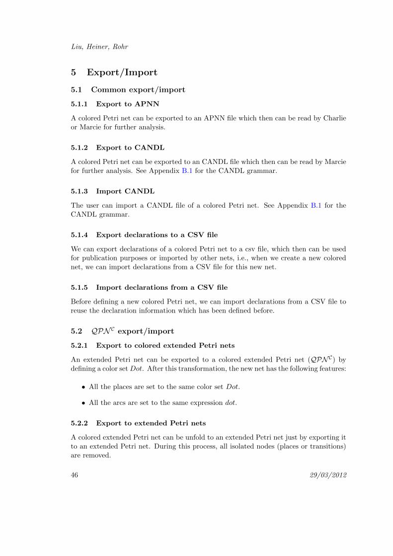
5 Export/Import
5.1 Common export/import
5.1.1 Export to APNN
A colored Petri net can be exported to an APNN file which then can be read by Charlieor Marcie for further analysis.
5.1.2 Export to CANDL
A colored Petri net can be exported to an CANDL file which then can be read by Marciefor further analysis. See Appendix B.1 for the CANDL grammar.
5.1.3 Import CANDL
The user can import a CANDL file of a colored Petri net. See Appendix B.1 for theCANDL grammar.
5.1.4 Export declarations to a CSV file
We can export declarations of a colored Petri net to a csv file, which then can be usedfor publication purposes or imported by other nets, i.e., when we create a new colorednet, we can import declarations from a CSV file for this new net.
5.1.5 Import declarations from a CSV file
Before defining a new colored Petri net, we can import declarations from a CSV file toreuse the declaration information which has been defined before.
5.2 QPN C export/import
5.2.1 Export to colored extended Petri nets
An extended Petri net can be exported to a colored extended Petri net (QPN C) bydefining a color setDot. After this transformation, the new net has the following features:
• All the places are set to the same color set Dot.
• All the arcs are set to the same expression dot.
5.2.2 Export to extended Petri nets
A colored extended Petri net can be unfold to an extended Petri net just by exporting itto an extended Petri net. During this process, all isolated nodes (places or transitions)are removed.
46 29/03/2012

The Manual for Colored Petri Nets in Snoopy
5.2.3 Export to colored stochastic Petri nets
A colored extended Petri net (QPN C) can be transformed into a colored stochasticPetri net. All information is kept during this process, and all rate functions for thetransformed SPN C are set to MassAction(1).
5.2.4 Export the structure to extended Petri nets
The structure of a colored extended Petri net (QPN C) can be exported to an extendedPetri net. In this specific case, there is no unfolding involved.
5.2.5 Export to CPN tools
A colored extended Petri net (QPN C) can be transformed to a file read by CPN tools[CPN11]. After this transformation, sometimes we have to modify the arc or guardexpressions to let them comply with the syntax of CPN tools. In summary, the followingpoints should be noted:
• Modify user-defined functions in the declaration part,
• Change the syntax of predicates to the if-then-else syntax supported by CPN tools,
• Replace the operators of successor, predecessor etc. with user-defined functions,
• Modify arc expressions that belong to the union type.
5.3 SPN C export/import
5.3.1 Export to colored stochastic Petri nets
A stochastic Petri net can be exported to a colored stochastic Petri net by defining acolor set Dot. After this transformation, the new net has the following features:
• All the places are set to the same color set Dot.
• All the arcs are set to the same expression dot.
5.3.2 Export to stochastic Petri nets
A colored stochastic Petri net can be unfolded to a stochastic Petri net just by exportingit to a stochastic Petri net. During this process, all isolated nodes (places or transitions)are removed.
5.3.3 Export to colored extended Petri nets
A colored stochastic Petri net can be transformed to a colored extended Petri net. Afterthis transformation, all information about rate functions is lost.
BTU CSR 02-12 47

Liu, Heiner, Rohr
5.3.4 Export to colored continuous/hybrid Petri nets
A colored stochastic Petri net can be transformed to a colored continuous/hybrid Petrinet.
5.3.5 Export the structure to stochastic Petri nets
The structure of a colored stochastic Petri net (SPN C) can be exported to a stochasticPetri net. In this specific case, there is no unfolding involved.
5.3.6 Export to CPN tools
A colored stochastic Petri net (SPN C) can be transformed to a file read by CPN tools[CPN11]. After this transformation, sometimes we have to modify the arc or guardexpressions to let them comply with the syntax of CPN tools.
5.4 CPN C export/import
5.4.1 Export to colored continuous Petri nets
A continuous Petri net can be exported to a colored continuous Petri net by defining acolor set Dot. After this transformation, the new net has the following features:
• All the places are set to the same color set Dot.
• All the arcs are set to the same expression dot.
5.4.2 Export to continuous Petri nets
A colored continuous Petri net can be unfolded to a continuous Petri net just by exportingit to a continuous Petri net. During this process, all isolated nodes (places or transitions)are removed.
5.4.3 Export to colored stochastic/hybrid Petri nets
A colored continuous Petri net can be transformed to a colored stochastic/hybrid Petrinet.
5.4.4 Export the structure to continuous Petri nets
The structure of a colored continuous Petri net (CPN C) can be exported to a continuousPetri net. In this specific case, there is no unfolding involved.
48 29/03/2012

The Manual for Colored Petri Nets in Snoopy
5.5 GHPN C export/import
5.5.1 Export to colored hybrid Petri nets
A hybrid Petri net can be exported to a colored hybrid Petri net by defining a color setDot. After this transformation, the new net has the following features:
• All the places are set to the same color set Dot.
• All the arcs are set to the same expression dot.
5.5.2 Export to hybrid Petri nets
A colored hybrid Petri net can be unfolded to a hybrid Petri net just by exporting it toa continuous Petri net. During this process, all isolated nodes (places or transitions) areremoved.
5.5.3 Export to colored stochastic/continuous Petri nets
A colored hybrid Petri net can be transformed to a colored stochastic/continuous Petrinet.
5.5.4 Export the structure to hybrid Petri nets
The structure of a colored hybrid Petri net (GHPN C) can be exported to a hybrid Petrinet. In this specific case, there is no unfolding involved.
BTU CSR 02-12 49

Liu, Heiner, Rohr
6 Examples
6.1 Cooperative ligand binding
We consider an example of the binding of oxygen to the four subunits of a hemoglobinheterotetramer. The hemoglobin heterotetramer in the high and low affinity state bindsto none, one, two, three or four oxygen molecules. Each of the ten states is repre-sented by a place and oxygen feeds into the transitions that sequentially connect therespective places. The qualitative Petri net model is illustrated in Figure 33 (taken from[MWW10]).
HbO2L_4 HbO2H_4
HbO2H_0HbO2L_0
O2
4
O2
4
O2
4
O2
4
O2
4
O2
4
O2
4
O2
4
O2
4
O2
4
O2
4
O2
4
HbO2H_1HbO2L_1
HbO2H_2HbO2L_2
HbO2L_3HbO2H_3
Figure 33: Cooperative binding of oxygen to hemoglobin represented as a Petri netmodel [MWW10]. For clarity, oxygen is represented in the form of multiple copies(logical places) of one place.
Now we begin to construct a colored Petri net model for Figure 33. For this, we first
50 29/03/2012
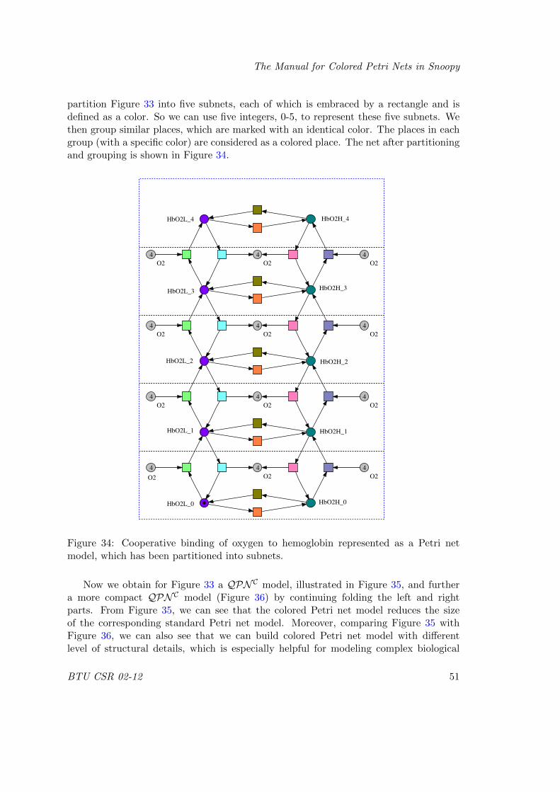
The Manual for Colored Petri Nets in Snoopy
partition Figure 33 into five subnets, each of which is embraced by a rectangle and isdefined as a color. So we can use five integers, 0-5, to represent these five subnets. Wethen group similar places, which are marked with an identical color. The places in eachgroup (with a specific color) are considered as a colored place. The net after partitioningand grouping is shown in Figure 34.
HbO2L_4 HbO2H_4
HbO2H_0HbO2L_0
O2
4
O2
4
O2
4
O2
4
O2
4
O2
4
O2
4
O2
4
O2
4
O2
4
O2
4
O2
4
HbO2H_1HbO2L_1
HbO2H_2HbO2L_2
HbO2L_3HbO2H_3
Figure 34: Cooperative binding of oxygen to hemoglobin represented as a Petri netmodel, which has been partitioned into subnets.
Now we obtain for Figure 33 a QPN C model, illustrated in Figure 35, and furthera more compact QPN C model (Figure 36) by continuing folding the left and rightparts. From Figure 35, we can see that the colored Petri net model reduces the sizeof the corresponding standard Petri net model. Moreover, comparing Figure 35 withFigure 36, we can also see that we can build colored Petri net model with differentlevel of structural details, which is especially helpful for modeling complex biological
BTU CSR 02-12 51

Liu, Heiner, Rohr
systems. After automatic unfolding, these two colored models yield exactly the samePetri net model as given in Figure 33, i.e., the colored models and the uncolored modelare equivalent. The declarations for these two QPN C models of the cooperative ligandbinding are given in Table 5.
O2
4
4‘dotDot
HbO2L1‘0
HbO2
HbO2H
HbO2
t1 [x<>4] t2 [x<>4] t3 [x<>4] t4 [x<>4]
t5
t6
dot dot dot dot
x+1 x x x+1
x x
xx
x+1 x x x+1
Figure 35: QPN C model for the cooperative binding of oxygen to hemoglobin, given asa standard Petri net in Figure 33. For declarations of color sets and variables, see 5.
Table 5: Declarations for the QPN C models of the cooperative ligand binding.
Declarations
colorset Dot = dot;
colorset HbO2 = int with 0-4;
colorset Level = enum with H,L;
colorset P = product with HbO2 × Level;
variable x: HbO2;
variable y: Level;
Function P Fun1(HbO2 x, Level y) {[y=L]1`(x+1,y)++[y=H]1`(x,y)};
Function P Fun2(HbO2 x, Level y) {[y=H]1`(x+1,y)++[y=L]1`(x,y)};
Besides, we give another colored model (see Figure 37), which uses user-definedfunctions and is equivalent to Figure 36. In this model, we define two functions Fun1 andFun2 to replace lengthy expressions. See Table 5 for details about these two functions.
From these colored nets, we can also see that the folding operation does reduce the
52 29/03/2012

The Manual for Colored Petri Nets in Snoopy
O2
4
4‘dot Dot
HbO211‘(0,L) P
t1 [x<>4] t2 [x<>4]
t3t4
[y=L]dot
[y=H]dot
[y=L]dot
[y=H]dot
[y=L]1‘(x+1,y)++
[y=H]1‘(x,y)
[y=H]1‘(x+1,y)++
[y=L]1‘(x,y)
[y=H]1‘(x+1,y)++
[y=L]1‘(x,y)
[y=L]1‘(x+1,y)++
[y=H]1‘(x,y)
[y=H]1‘(x,L)
[y=H]1‘(x,y)
[y=L]1‘(x,y)
[y=L]1‘(x,H)
Figure 36: QPN C model for the cooperative binding of oxygen to hemoglobin, given asa standard Petri net in Figure 33. For declarations of color sets and variables, see Table5.
O2
4
4‘dot Dot
HbO211‘(0,L) P
t1 [x<>4] t2 [x<>4]
t3t4
[y=L]dot
[y=H]dot
[y=L]dot
[y=H]dot
Fun1(x,y)
Fun2(x,y)
Fun2(x,y)Fun1(x,y)
[y=H]1‘(x,L)
[y=H]1‘(x,y)
[y=L]1‘(x,y)
[y=L]1‘(x,H)
Figure 37: Another QPN C model for the cooperative binding of oxygen to hemoglobin,which uses user-defined functions and is equivalent to Figure 36. For declarations ofcolor sets and variables, see Table 5.
BTU CSR 02-12 53

Liu, Heiner, Rohr
size of the net description for the prize of more complicated inscriptions. The graphiccomplexity is reduced, but the annotations of nodes and edges creates a new challenge.This is not unexpected since a more concise write-up must rely on more complex com-ponents. Therefore, it is necessary to build a colored Petri net model at a suitable levelof structural details.
6.2 Repressilator
In this section, we will demonstrate the SPN C using an example of a synthetic circuit- the repressilator, which is an engineered synthetic system encoded on a plasmid, anddesigned to exhibit oscillations [EL00]. The repressilator system is a regulatory cycleof three genes, for example, denoted by g a, g b and g c, where each gene represses itssuccessor, namely, g a inhibits g b, g b inhibits g c, and g c inhibits g a. This negativeregulation is realized by the repressors, p a, p b and p c, generated by the genes g a,g b and g c respectively [LB07].
As our purpose is to demonstrate the SPN C , we only consider a relatively simplemodel of the repressilator, which was built as a stochastic π-machine in [BCP08]. Basedon that model, we build a stochastic Petri net model (Figure 38), and further a SPN Cmodel for the repressilator (shown on the left hand of Figure 39). This colored modelwhen unfolded yields the same uncolored Petri net model in Figure 38.
blocked_a
proteine_a
gene_a
blocked_b
proteine_b
gene_b
blocked_c
proteine_c
gene_c
block_a
block_a
degrade
unblockgenerate
degrade
unblockgenerate
degrade
unblockgenerateblock_b
block_b
block_c
block_c
Figure 38: Stochastic Petri net model for the repressilator. The highlighted transitionsare logical transitions.
For the SPN C model in Figure 39, there are three colors, a, b, and c to distinguishthree similar components in Figure 38. The predecessor operator “-” in the arc expression−x returns the predecessor of x in an ordered finite color set. If x is the first color, thenit returns the last color.
As described above, the SPN C will be automatically unfolded to a stochastic Petrinet, and can be simulated with different simulation algorithms. On the right hand ofFigure 39 a snapshot of a simulation run result is given. The rate functions are given inTable 6 (coming from [PC07]). The SPN C model exhibits the same behavior comparedwith that in [PC07].
54 29/03/2012

The Manual for Colored Petri Nets in Snoopy
blocked
Gene
proteine
Gene
gene
31`all()
Gene
block
degrade
unblockgenerate
x
xx
x
xxx
x
-x
-x
Declarations:
colorset Gene=enum with a,b,c;
variable x:Gene;
-0.0e+000 2.0e+004 4.0e+004 6.0e+004 8.0e+004 1.0e+005-020406080100120 proteine_aproteine_bproteine_cStochastic Result: repressilatorex.colstochpn
Time
Val
ue
Figure 39: SPN C model of the standard Petri net given in Figure 38, and one simulationrun plot for the repressilator. For rate functions, see Table 6.
Table 6: Rate functions for the SPN C model of the repressilator.
Transition Rate function
generate 0.1 ∗ gene
block 1.0 ∗ proteine
unblock 0.0001 ∗ blocked
degrade 0.001 ∗ proteine
From Figure 39, we can see that the SPN C model reduces the size of the originalstochastic Petri net model to one third. More importantly, when other similar subnetshave to be added, the model structure does not need to be modified and what has to bedone is only to add extra colors.
For example, we consider the generalized repressilator with an arbitrary number nof genes in the loop that is presented in [MHE+06]. To build its SPN C model, we justneed to modify the color set as n colors, and do not need to modify anything else. Forexample, Figure 40 gives the conceptual graph of the generalized repressilator with n = 9(on the left hand), and one simulation plot (on the right hand), whose rate functions arethe same as in Table 6. Please note, the SPN C model for the generalized repressilatoris the same as the one for the three-gene repressilator, and the only difference is that wedefine the color set as n colors rather than 3 colors. This demonstrates a big advantage
BTU CSR 02-12 55

Liu, Heiner, Rohr
of color Petri nets, that is, to increase the colors means to increase the size of the net.
-0 20000 40000 60000 80000 100000-020406080100120140160 proteine_aproteine_bproteine_cproteine_dproteine_eproteine_fproteine_gproteine_hproteine_i
Stochastic Result: repressilatorex.colstochpn
Time
Val
ue
Figure 40: Conceptual graph and one simulation run plot for the repressilator with 9genes.
6.3 Where to find more examples
In [GLG+11], [GLT+11], colored (both stochastic and continuous) Petri nets have beenused to describe the phenomenon of Planar Cell Polarity (PCP) signaling in Drosophilawing. Two colored models (abstract and refined) has been developed, which model agroup of cells on a two-dimensional grid, corresponding to a fragment of the wing tissue.Moreover each cell is partitioned into seven virtual compartments, so these two modelshas a two-level hierarchy. In addition, these models involve product color sets, subsetsof color sets, user-defined functions and etc.
More case studies can be found in [GH11], [Liu12], e.g.
• Gradient,
• Dictyostelium colony formation,
• Phase variation in bacterial colony growth,
• C. Elegans vulval development,
• Coupled Ca2+ channels,
• Membrane systems.
56 29/03/2012

The Manual for Colored Petri Nets in Snoopy
References
[ASAP11] ASAP: http://www.daimi.au.dk/~ascoveco/asap.html (2011)
[BCP08] R. Blossey, L. Cardelli, A. Phillips: Compositionality, Stochasticity and Coop-erativity in Dynamic Models of Gene Regulation. HFSP Journal. 2(1), 17-28 (2008)
[BNF11] BNF: http://en.wikipedia.org/wiki/Backus_Naur_Form (2011)
[Cha11] Charlie - a Software Tool to Analyze Place/Transition Nets: http://www-dssz.informatik.tu-cottbus.de/DSSZ/Software/Charlie (2011)
[CPN11] CPN tools: http://cpntools.org/ (2011)
[EL00] M.B. Elowitz, S. Leibler: A Synthetic Oscillatory Network of TranscriptionalRegulators. Nature. 403, 335-338 (2000)
[Fra09] A. Franzke: Charlie 2.0 - a Multi-Threaded Petri Net Analyzer. Diploma Thesis,Brandenburg University of Technology Cottbus. (2009)
[GH11] D. Gilbert, M. Heiner: Petri nets for multiscale Systems Biology: http://
multiscalepn.brunel.ac.uk (2011)
[GHL07] D. Gilbert, M. Heiner, S. Lehrack : A Unifying Framework for Modelling andAnalysing Biochemical Pathways Using Petri Nets. Proc. International Conference onComputational Methods in Systems Biology. LNCS/LNBI, 4695, 200-216 (2007)
[Gil77] D.T. Gillespie: Exact Stochastic Simulation of Coupled Chemical Reactions.Journal of Physical Chemistry. 81(25), 2340-2361 (1977)
[GL79] H.J. Genrich, K. Lautenbach: The Analysis of Distributed Systems by Means ofPredicate/Transition-Nets. Semantics of Concurrent Computation. LNCS, 70, 123-146(1979)
[GL81] H.J. Genrich, K. Lautenbach: System Modelling with High-Level Petri Nets.Theoretical Computer Science. 13(1), 109-135 (1981)
[GLG+11] Q. Gao, F. Liu, D. Gilbert, M. Heiner, D. Tree: A Multiscale Approachto Modelling Planar Cell Polarity in Drosophila Wing using Hierarchically ColouredPetri Nets. Proc. 9th International Conference on Computational Methods in SystemsBiology (CMSB 2011). ACM digital library (2011)
[GLT+11] Q. Gao, F. Liu, D. Tree, D. Gilbert: Multi-cell Modeling Using ColouredPetri Nets Applied to Plannar Cell Polarity. Proc. 2th International Workshop onBiological Processes & Petri nets. CEUR Workshop Proceedings, 724, 135-150 (2011)
[HH11] M. Herajy, M. Heiner: Hybrid Representation and Simulation of Stiff Biochemi-cal Networks through Generalised Hybrid Petri Nets. Technical Report, BrandenburgUniversity of Technology Cottbus, Department of Computer Science (2011)
BTU CSR 02-12 57

Liu, Heiner, Rohr
[HLG+09] M. Heiner, S. Lehrack, D. Gilbert, W. Marwan: Extended Stochastic PetriNets for Model-based Design of Wetlab Experiments. Transaction on ComputationalSystems Biology XI. LNCS/LNBI, 5750, 138-163 (2009)
[HRR+08] M. Heiner, R. Richter, C. Rohr, M. Schwarick: Snoopy - A Tool to Designand Execute Graph-Based Formalisms. [Extended Version]. Petri Net Newsletter. 74,8-22 (2008)
[Jen81] K. Jensen: Coloured Petri Nets and the Invariant-Method. Theoretical Com-puter Science. 14(3), 317-336 (1981)
[JKW07] K. Jensen, L.M. Kristensen, L.M. Wells: Coloured Petri Nets and CPN Toolsfor Modelling and Validation of Concurrent Systems. International Journal on Soft-ware Tools for Technology Transfer. 9(3/4), 213-254 (2007)
[LB07] A. Loinger, O. Biham: Stochastic Simulations of the Repressilator Circuit. Phys-ical Review. 76(5), 051917(9) (2007)
[Liu12] F. Liu: Colored Petri Nets for Systems Biology, Ph.D. Thesis, BTU Cottbus,Dep. of CS, (2012)
[Mar11] Marcie - a Tool for Qualitative and Quantitative Analysis of General-ized Stochastic Petri Nets. http://www-dssz.informatik.tu-cottbus.de/DSSZ/
Software/Marcie (2011)
[MC210] MC2 website: MC2 - A PLTL Model Checker. University of Glasgow, http://www.brc.dcs.gla.ac.uk/~drg/courses/sysbiomres/software/mc2 (2010)
[MHE+06] S. Muller, J. Hofbauer, L. Endler, C. Flamm, S. Widder, P. Schuster: AGeneralized Model of the Repressilator. Journal of Mathematical Biology. 53, 905-937(2006)
[MWW10] W. Marwan, A. Wagler, R. Weismantel: Petri Nets as a Framework forthe Reconstruction and Analysis of Signal Transduction Pathways and RegulatoryNetworks. Natural Computing. 10(2), 639-654 (2010)
[MRH12] W. Marwan, C. Rohr, M. Heiner: Petri nets in Snoopy: A unifying frameworkfor the graphical display, computational modelling, and simulation of bacterial reg-ulatory networks, in Jv Helden and A Toussaint and D Thieffry (Eds.), Methods inMolecular Biology – Bacterial Molecular Networks, chapter 21, Humana Press, seriesMethods in Molecular Biology, Vol. 804, pp. 409–437 (2012)
[PC07] A. Phillips, L. Cardelli: Efficient, Correct Simulation of Biological Processes inthe Stochastic Pi-Calculus. Proc. Computational Methods in Systems Biology. LNCS,4695, 184-199 (2007)
[RMH10] C. Rohr, W. Marwan, M. Heiner: Snoopy - a Unifying Petri Net Frameworkto Investigate Biomolecular Networks: Bioinformatics. 26(7), 974-975 (2010)
58 29/03/2012

The Manual for Colored Petri Nets in Snoopy
[SH09] M. Schwarick, M. Heiner: CSL Model Checking of Biochemical Networks withInterval Decision Diagrams. Proc. 7th International Conference on ComputationalMethods in Systems Biology (CMSB 2009), LNBI 5688, 296-312 (2009)
BTU CSR 02-12 59

Liu, Heiner, Rohr
A Annotation Language
A.1 Introduction to BNF
A Backus-Naur Form (BNF) specification is a set of derivation rules [BNF11], writtenas
〈symbol〉 ::= expression
| “terminal”
where:
1. 〈symbol〉 is a nonterminal; expression consists of one or more sequences of symbols;more sequences are separated by the vertical bar, | , indicating a choice, the wholebeing a possible substitution for the symbol on the left.
2. Symbols that never appear on a left side are terminals, which are notated by usingthe double quotation marks “ ”.
3. Symbols that appear on a left side are non-terminals.
4. ::= means “is defined as”.
5. ⊥ means “empty” or “null”.
60 29/03/2012

The Manual for Colored Petri Nets in Snoopy
A.2 BNF for the data type definition
〈Type〉 ::= 〈SimpleType〉 | 〈CompoundType〉〈SimpleType〉 ::= 〈TypeIdentifier〉 | 〈StructuredType〉
〈TypeIdentifier〉 ::= 〈UnsignedInteger〉 | 〈Boolean〉 | 〈String〉〈UnsignedInteger〉 ::= “int”
〈Boolean〉 ::= “bool”
〈String〉 ::= “string”
〈StructuredType〉 ::= 〈Enumeration〉 | 〈Index〉〈Enumeration〉 ::= 〈IdentifierList〉〈IdentifierList〉 ::= 〈Identifier〉 | 〈IdentifierList〉“,”〈Identifier〉
〈Index〉 ::= 〈Identifier〉“[”〈IndexSpecifier〉“]”
〈IndexSpecifier〉 ::= “int”
〈CompoundType〉 ::= 〈Product〉 | 〈Union〉〈Product〉 ::= 〈Type〉“×”〈Type〉 | 〈Product〉“×”〈Type〉〈Union〉 ::= 〈Type〉 | 〈Union〉“,”〈Type〉
BTU CSR 02-12 61

Liu, Heiner, Rohr
A.3 BNF for the annotation language
〈ColorExpr〉 ::= 〈MultiSetExpr〉〈MultiSetExpr〉 ::= 〈Predicate〉 | 〈MultiSetExpr〉〈MSAdditionOp〉〈Predicate〉〈MSAdditionOp〉 ::= “++”
〈Predicate〉 ::= 〈SeparatorExpr〉 | “[”〈OrExpr〉“]”〈SeparatorExpr〉〈SeparatorExpr〉 ::= 〈TupleExpr〉 | 〈SeparatorExpr〉〈SeparatorOp〉〈TupleExpr〉〈SeparatorOp〉 ::= “`”
〈TupleExpr〉 ::= 〈OrExpr〉 | “(”〈CommaExpr〉“)”
〈CommaExpr〉 ::= 〈TupleExpr〉 | 〈CommaExpr〉〈CommaOp〉〈TupleExpr〉〈CommaOp〉 ::= “,”
〈OrExpr〉 ::= 〈AndExpr〉 | 〈OrExpr〉〈OrOp〉〈AndExpr〉〈OrOp〉 ::= “|”
〈AndExpr〉 ::= 〈EqualExpr〉 | 〈AndExpr〉〈AndOp〉〈EqualExpr〉〈AndOp〉 ::= “&”
〈EqualExpr〉 ::= 〈RelationExpr〉 | 〈EqualExpr〉〈EqualOp〉〈RelationExpr〉〈EqualOp〉 ::= “=” | “<>”
〈RelationExpr〉 ::= 〈AddExpr〉 | 〈RelationExpr〉〈RelationOp〉〈AddExpr〉〈RelationOp〉 ::= “<” | “<=” | “>=” | “>”
〈AddExpr〉 ::= 〈MultiplicityExpr〉 | 〈AddExpr〉〈AddOp〉〈MultiplicityExpr〉〈AddOp〉 ::= “+” | “-”
〈MultiplicityExpr〉 ::= 〈UnaryExpr〉 | 〈MultiplicityExpr〉〈MultiplicityOp〉〈UnaryExpr〉〈MultiplicityOp〉 ::= “*” | “/” | “%” | “ˆ”
〈UnaryExpr〉 ::= 〈PostfixExpr〉 | 〈UnaryOp〉〈PostfixExpr〉〈UnaryOp〉 ::= “+” | “-” | “@” | “!”
〈PostfixExpr〉 ::= 〈AtomExpr〉 | 〈PostfixExpr〉“[”〈AtomExpr〉“]”
| 〈PostfixExpr〉“:”〈AtomExpr〉〈AtomExpr〉 ::= 〈Constant〉 | 〈Variable〉 | 〈Function〉 | “(”〈ColorExpr〉“)”
〈Constant〉 ::= 〈Integer〉 | 〈String〉〈Variable〉 ::= 〈Identifier〉〈Function〉 ::= 〈Identifier〉“(”〈ArgumentList〉“)”“{”〈FunctionBody〉“}”
〈ArgumentList〉 ::= 〈OrExpr〉 | 〈ArgumentList〉〈CommaOp〉〈OrExpr〉〈FunctionBody〉 ::= 〈MultiSetExpr〉
〈Integer〉 ::= 〈Digit〉 | 〈Integer〉〈Digit〉〈String〉 ::= 〈LetterOrDigit〉 | 〈String〉〈LetterOrDigit〉
〈Identifier〉 ::= 〈Letter〉 | 〈Identifier〉〈LetterOrDigit〉
62 29/03/2012

The Manual for Colored Petri Nets in Snoopy
〈LetterOrDigit〉 ::= 〈Letter〉 | 〈Digit〉〈Digit〉 ::= “0–9”
〈Letter〉 ::= “a–zA–Z ”
BTU CSR 02-12 63

Liu, Heiner, Rohr
B Colored Abstract Net Definition Language (CANDL)
B.1 BNF
〈Start〉 ::= 〈NetType〉“[”〈Identifier〉“]”“{”〈Net〉“}”〈NetType〉 ::= “colpn” | “colxpn” | “colcpn” | “colhpn”
| “colspn” | “colgspn” | “colxspn”
〈Net〉 ::= 〈Constants〉〈SimpleColorsets〉〈CompoundColorsets〉〈Variables〉〈Functions〉〈Places〉〈Observers〉〈Transitions〉
〈Constants〉 ::= “constants:”〈ConstList〉〈ConstList〉 ::= ⊥ | 〈ConstDef〉 | 〈ConstDef〉〈ConstList〉〈ConstDef〉 ::= 〈ConstType〉〈Identifier〉〈ConstInit〉“;”
〈ConstType〉 ::= “int” | “double” | “bool” | “string”
〈ConstInit〉 ::= ⊥ | “=”〈ConstExpr〉
〈SimpleColorsets〉 ::= “simplecolorsets:”〈SimpleCsList〉〈SimpleCsList〉 ::= 〈SimpleCsDef〉 | 〈SimpleCsDef〉〈SimpleCsList〉〈SimpleCsDef〉 ::= 〈SimpleCsType〉〈Identifier〉〈SimpleCsInit〉“;”
〈SimpleCsType〉 ::= “dot” | “int” | “bool” | “string” | “enum” | “index”
| 〈SimpleColorset〉〈SimpleCsInit〉 ::= 〈DotCsInit〉 | 〈IntCsInit〉 | 〈BoolCsInit〉 | 〈StringCsInit〉
| 〈EnumCsInit〉 | 〈IndexCsInit〉 | 〈Predicate〉〈DotCsInit〉 ::= “dot”
〈IntCsInit〉 ::= 〈IntCsDef〉 | 〈IntCsDef〉〈IntCsDelim〉〈IntCsInit〉〈IntCsDef〉 ::= 〈Integer〉 | 〈Constant〉
〈IntCsDelim〉 ::= “,” | “-”
〈BoolCsInit〉 ::= “true”“,”“false”
〈StringCsInit〉 ::= 〈String〉 | 〈String〉“,”〈StringCsInit〉〈EnumCsInit〉 ::= 〈Identifier〉 | 〈Identifier〉“,”〈EnumCsInit〉
64 29/03/2012

The Manual for Colored Petri Nets in Snoopy
〈IndexCsInit〉 ::= 〈Identifier〉“[”〈Integer〉“,”〈Integer〉“]”
〈CompoundColorsets〉 ::= “compoundcolorsets:”〈CompoundCsList〉〈CompoundCsList〉 ::= ⊥ | 〈CompoundCsDef〉 | 〈CompoundCsDef〉〈CompoundCsList〉〈CompoundCsDef〉 ::= 〈CompoundCsType〉〈Identifier〉〈CompoundCsInit〉“;”
〈CompoundCsType〉 ::= “product” | “union” | 〈CompoundColorset〉〈CompoundCsInit〉 ::= 〈CsComponents〉 | 〈Predicate〉〈CsComponents〉 ::= 〈Colorset〉 | 〈Colorset〉“,”〈CsComponents〉
〈Variables〉 ::= “variables:”〈VariableList〉〈VariableList〉 ::= ⊥ | 〈VariableDef〉 | 〈VariableDef〉〈VariableList〉〈VariableDef〉 ::= 〈Colorset〉〈Identifier〉“;”
〈Functions〉 ::= “functions:”〈FunctionList〉〈FunctionList〉 ::= ⊥ | 〈FunctionDef〉 | 〈FunctionDef〉〈FunctionsList〉〈FunctionDef〉 ::= 〈FunctionType〉〈Identifier〉“(”〈FunctionParams〉“)”〈FunctionBody〉“;”
〈FunctionType〉 ::= 〈SimpleCsType〉 | 〈CompoundCsType〉〈FunctionParams〉 ::= ⊥ | 〈FunctionParam〉 | 〈FunctionParam〉“,”〈FunctionParams〉〈FunctionParam〉 ::= 〈FunctionType〉〈Identifier〉〈FunctionBody〉 ::= “{”〈ColorExpr〉“}”
〈Places〉 ::= “places:”〈PlaceList〉〈PlaceList〉 ::= 〈PlaceDef〉 | 〈PlaceDef〉〈PlaceList〉〈PlaceDef〉 ::= 〈PlaceType〉〈Colorset〉〈Identifier〉〈PlaceInit〉“;”
〈PlaceType〉 ::= ⊥ | “discrete:” | “continuous:”
〈PlaceInit〉 ::= “=”“{”〈Assignments〉“}”〈Assignments〉 ::= 〈Assignment〉 | 〈Assignment〉“,”〈Assignments〉〈Assignment〉 ::= “{”〈ConstExpr〉“`”〈ColorExpr〉“}”
〈Observers〉 ::= “observers:”〈ObserverList〉〈ObserverList〉 ::= ⊥ | 〈ObserverDef〉 | 〈ObserverDef〉〈ObserverList〉〈ObserverDef〉 ::= 〈Identifier〉“=”〈ObserverInit〉“;”
〈ObserverInit〉 ::= “{”〈Predicate〉“,”〈ObserverFunc〉“}”〈ObserverFunc〉 ::= 〈ObserverOp〉“(”〈CsComponents〉“)”
〈ObserverOp〉 ::= “+”
BTU CSR 02-12 65

Liu, Heiner, Rohr
〈Transitions〉 ::= “transitions:”〈TransList〉〈TransList〉 ::= 〈TransDef〉 | 〈TransDef〉〈TransList〉〈TransDef〉 ::= 〈TransType〉〈Identifier〉〈Guard〉
“:”〈ConditionList〉“:”〈UpdateList〉〈RateFunctionList〉“;”
〈TransType〉 ::= “stochastic:” | “immediate:” | “deterministic:”
| “scheduled:” | “continuous:”
〈Guard〉 ::= ⊥ | “[”〈Predicate〉“]”
〈ConditionList〉 ::= ⊥ | 〈ConditionDef〉 | 〈ConditionDef〉“&”〈ConditionList〉〈ConditionDef〉 ::= “[”“{”〈ColorExpr〉“}”“<=”〈Place〉“<”“{”〈ColorExpr〉“}”“]”
| “[”“{”〈ColorExpr〉“}”“<=”〈Place〉“]”
| “[”“{”〈ColorExpr〉“}”“=”〈Place〉“]”
| “[”“{”〈ColorExpr〉“}”“>”〈Place〉“]”
| “[”〈Place〉“<”“{”〈ColorExpr〉“}”“]”
| “[”〈Place〉“=”“{”〈ColorExpr〉“}”“]”
| “[”〈Place〉“>=”“{”〈ColorExpr〉“}”“]”
| “[”〈Place〉“]”
〈UpdateList〉 ::= ⊥ | 〈UpdateDef〉 | 〈UpdateDef〉“&”〈UpdateList〉〈UpdateDef〉 ::= “[”〈Place〉〈UpdateOp〉“{”〈ColorExpr〉“}”“]”
〈UpdateOp〉 ::= “+” | “-” | “=”
〈RateFunctionList〉 ::= ⊥ | “:”“{”〈RateFunctions〉“}”〈RateFunctions〉 ::= 〈RateFunction〉 | 〈RateFunction〉“,”〈RateFunctions〉〈RateFunction〉 ::= “{”〈Predicate〉“:”〈RateFunctionDef〉“}”
〈RateFunctionDef〉 ::= 〈ColorPattern〉 | 〈Pattern〉 | 〈ArithmeticFunction〉〈ColorPattern〉 ::= “[”〈ColorExpr〉“]” | “#”“(”〈Identifier〉“)”
〈Pattern〉 ::= 〈Func1Param〉“(”〈ArithmeticFunction〉“)”
| 〈Func2Param〉“(”〈ArithmeticFunction〉“,”〈ArithmeticFunction〉“)”
| 〈Func2Param〉“(”〈ArithmeticFunction〉“,”〈ArithmeticFunction〉“)”
| 〈ArithmeticFunction〉“,”〈ArithmeticFunction〉“,”〈ArithmeticFunction〉〈Func1Param〉 ::= “MassAction”
〈Func2Param〉 ::= “LevelInterpretation”
| “MichaelisMenten”
| “Inhibit”
66 29/03/2012

The Manual for Colored Petri Nets in Snoopy
| “Read”
| “Equal”
〈ArithmeticFunction〉 ::= 〈Term〉 | 〈Term〉〈AddOp〉〈ArithmeticFunction〉〈AddOp〉 ::= “+” | “-”
〈Term〉 ::= 〈Factor〉 | 〈Factor〉〈MultOp〉〈Term〉〈MultOp〉 ::= “*” | “/” | “ˆ”
〈Factor〉 ::= 〈Atom〉 | “-”〈Factor〉〈Atom〉 ::= 〈Integer〉
| 〈Float〉| 〈Constant〉| 〈Place〉| “(”〈ArithmeticFunction〉“)”
| 〈UnOp〉“(”〈ArithmeticFunction〉“)”
| 〈BinOp〉“(”〈ArithmeticFunction〉“,”〈ArithmeticFunction〉“)”
〈UnOp〉 ::= “abs” | “exp” | “sqr” | “sqrt” | “floor”
| “ceil” | “sin” | “asin” | “cos” | “acos”
| “tan” | “atan” | “log10” | “log”
〈BinOp〉 ::= “pow” | “min” | “max”
〈Constant〉 ::= 〈Identifier〉 //name of a defined constant
〈SimpleColorset〉 ::= 〈Identifier〉 //name of a defined simple color set
〈CompoundColorset〉 ::= 〈Identifier〉 //name of a defined compound color set
〈Colorset〉 ::= 〈SimpleColorset〉 | 〈CompoundColorset〉〈Variable〉 ::= 〈Identifier〉 //name of a defined variable
〈Place〉 ::= 〈Identifier〉 //name of a defined place
BTU CSR 02-12 67

Liu, Heiner, Rohr
B.2 Example
For illustration we give the introductory dinning philosophers example, see Figure 1, inCANDL notation which has been generated by Snoopy’s export feature.
co lpn [ p h i l ]{cons tant s :
int N = 5 ;
s i m p l e c o l o r s e t s :dot Dot = dot ;int Ph i l s = 1−N;int Forks = 1−N;
compoundcolorsets :
v a r i a b l e s :Ph i l s x ;
f u n c t i o n s :Forks l e f t ( Ph i l s x )
{ x } ;Forks r i g h t ( Ph i l s x )
{ ( x%N)+1 } ;
p l a c e s :Ph i l s th ink ing = { {1` a l l ( ) } } ;Ph i l s wa i t ing = { {0` a l l ( ) } } ;Ph i l s ea t ing = { {0` a l l ( ) } } ;Ph i l s r e l e a s i n g = { {0` a l l ( ) } } ;Forks f o r k s = { {1` a l l ( ) } } ;
ob s e rve r s :
68 29/03/2012

The Manual for Colored Petri Nets in Snoopy
t r a n s i t i o n s :t a k e l e f t
:: [ wa i t ing + {x } ] & [ th ink ing − {x } ] & [ f o r k s − { l e f t ( x
) } ] ;t a k e r i g h t
:: [ e a t ing + {x } ] & [ wa i t ing − {x } ] & [ f o r k s − { r i g h t ( x )} ] ;
p u t r i g h t:: [ r e l e a s i n g + {x } ] & [ f o r k s + { r i g h t ( x ) } ] & [ ea t ing −{x } ] ;
p u t l e f t:: [ th ink ing + {x } ] & [ f o r k s + { l e f t ( x ) } ] & [ r e l e a s i n g −
{x } ] ;
}
BTU CSR 02-12 69