The Masses of the Milky Way and Andromeda Galaxies · The Masses of the Milky Way and Andromeda galaxies 3 parameter, in which σt is the tangential velocity dispersion. Now, β→

arX

iv:1

002.

4565

v1 [

astr

o-ph

.GA

] 24

Feb

201

0Mon. Not. R. Astron. Soc.000, 000–000 (0000) Printed 28 May 2018 (MN LATEX style file v2.2)

The Masses of the Milky Way and Andromeda Galaxies

Laura L. Watkins1, N. Wyn Evans1, Jin H. An2,3,4

1Institute of Astronomy, University of Cambridge, Madingley Road, Cambridge, CB3 0HA, UK2 National Astronomical Observatories, Chinese Academy of Sciences, A20 Datun Road, Chaoyang District, Beijing 100012, PR China,3 Dark Cosmology Centre, Niels Bohr Institutet, Københavns Universitet, Juliane Maries Vej 30, DK-2100 Copenhagen Ø, Denmark,4 Niels Bohr International Academy, Niels Bohr Institutet, Københavns Universitet, Blegdamsvej 17, DK-2100 Copenhagen Ø, Denmark.

28 May 2018

ABSTRACTWe present a family of robust tracer mass estimators to compute the enclosed mass of galaxyhaloes from samples of discrete positional and kinematicaldata of tracers, such as halo stars,globular clusters and dwarf satellites. The data may be projected positions, distances, lineof sight velocities or proper motions. The estimators all assume that the tracer populationhas a scale-free density and moves in a scale-free potentialin the region of interest. Thecircumstances under which the boundary terms can be discarded and the estimator convergesare derived. Forms of the estimator tailored for the Milky Way galaxy and for M31 are given.Monte Carlo simulations are used to quantify the uncertainty as a function of sample size.

For the Milky Way galaxy, the satellite sample consists of 26galaxies with line-of-sightvelocities. We find that the mass of the Milky Way within 300 kpc isM300 = 0.9±0.3×1012M⊙assuming velocity isotropy. However, the mass estimate is sensitive to the assumed anisotropyand could plausibly lie between 0.7 - 3.4 ×1012M⊙, if anisotropies implied by simulations orby the observations are used. Incorporating the proper motions of 6 Milky Way satellites intothe dataset, we findM300 = 1.4± 0.3× 1012M⊙. The range here if plausible anisotropies areused is still broader, from 1.2 - 2.7 × 1012M⊙. Note that our error bars only incorporate thestatistical uncertainty. There are much greater uncertainties induced by velocity anisotropyand by selection of satellite members.

For M31, there are 23 satellite galaxies with measured line-of-sight velocities, but onlyM33 and IC 10 have proper motions. We use the line of sight velocities and distances of thesatellite galaxies to estimate the mass of M31 within 300 kpcasM300 = 1.4± 0.4× 1012M⊙assuming isotropy. There is only a modest dependence on anisotropy, with the mass varyingbetween 1.3 - 1.6 × 1012M⊙. Incorporating the proper motion dataset does not change theresults significantly. Given the uncertainties, we conclude that the satellite data by themselvesyield no reliable insights into which of the two galaxies is actually the more massive.

Leo I has long been known to dominate mass estimates for the Milky Way due to its sub-stantial distance and line-of-sight velocity. We find that And XII and And XIV similarly dom-inate the estimated mass of M31. As such, we repeat the calculations without these galaxies,in case they are not bound – although on the balance of the evidence, we favour their inclusionin mass calculations.

Key words: galaxies: general – galaxies: haloes – galaxies: kinematics and dynamics – galax-ies: individual: M31 – dark matter

1 INTRODUCTION

The structure and extent of dark matter haloes have important im-plications for modern astrophysics, yet the determinationof suchproperties is a difficult task and the results are often conflicting. Aneat illustration is provided by the usage of Sagittarius Stream datato constrain the shape of the Milky Way dark halo. This has toldus that the halo is nearly spherical (Fellhauer et al. 2006),prolate(Helmi 2004), oblate (Johnston et al. 2005) or triaxial (Lawet al.2009) in nature! The Milky Way is the closest halo available for

our study, the availability of data has improved substantially in re-cent years, and yet we are not able to determine its shape reliably.

Similarly, we are unable to measure the masses of the MilkyWay, or its neighbour, the Andromeda Galaxy (M31) with any pre-cision. Despite their proximity to us, their masses remain sketchilydetermined and there is some controversy as to which halo is moremassive. Judged by criteria such as the surface brightness of thestellar halo or the numbers of globular clusters or the amplitude ofthe gas rotation curve, M31 is seemingly the more massive. Judgedby criteria such as the velocities of the satellite galaxiesand distant

c© 0000 RAS

http://arxiv.org/abs/1002.4565v1

2 Watkins, Evans& An

globulars or tidal radii of the dwarf spheroidals, then the Milky Wayis seemingly the more massive. For example, Evans et al. (2000) ar-gued that the M31 halo is roughly as massive as that of the MilkyWay, with the Milky Way marginally being the more massive of thetwo, while recent studies have found evidence favouring both theMilky Way (e.g. Evans & Wilkinson 2000; Gottesman et al. 2002)and M31 (e.g. Klypin et al. 2002; Karachentsev et al. 2009) asthemore massive galaxy.

The masses of both haloes within a few tens of kiloparsecsare reasonably well constrained by gas rotation curve data (e.g.Rohlfs & Kreitschmann 1988; Braun 1991). However, these dataonly sample the inner parts of the haloes. In order to probe fur-ther out, we must turn to the kinematics of the satellite popula-tions. Such tracers are a valuable tool for studying the darkmatterhaloes as their orbits contain important information abouttheir hostpotential. Distance, radial velocity and proper motion data can beused to constrain halo extent, mass and velocity anisotropy(seee.g. Little & Tremaine 1987; Kochanek 1996; Wilkinson & Evans1999).

The uncertainties in the mass estimates for the Milky Way andM31 are largely due to the fact that there is seldom proper motiondata available to complement distance and radial velocity informa-tion. With only one velocity component to work with, the eccentric-ities of the orbits are poorly constrained. Statistical methods mustbe applied to determine masses and these methods suffer greatlyfrom the small sample sizes available, even with the recent burst ofsatellite discoveries associated with both galaxies.

The projected mass estimator was introduced byBahcall & Tremaine (1981). They assumed that only projecteddistance and line-of-sight velocity information was available.The estimator is also contained in the study of White (1981) onscale-free ensembles of binary galaxies. The analysis was extendedby Heisler et al. (1985) and further modified by Evans et al. (2003)to consider the case of tracer populations. These previous studiessuccessfully used the mass estimator to weigh M31. However,inits present form, the mass estimator is ill-suited for application tothe Milky Way and such a study has not yet been attempted.

Here, we develop alternative forms of the estimator, andanalyse the conditions under which they are valid. In addition,the census of satellites around M31 has increased significantly(Zucker et al. 2004, 2007; Martin et al. 2006; Majewski et al.2007;Ibata et al. 2007; Irwin et al. 2008; McConnachie et al. 2008)sincethe last studies of this type were attempted and so we have moredata at our disposal. Hence, we apply our estimator to M31 withthese new data.

2 MASS ESTIMATORS

The projected mass estimator (Bahcall & Tremaine 1981) takes theform

M =CG

⟨

v2losR⟩

=CG

1N

N∑

i=1

v2los,iRi (1)

for a set ofN tracers objects (e.g planetary nebulae, stars, globularclusters, dwarf spheroidal galaxy satellites) with line-of-sight ve-locitiesvlos and projected distancesR. Here,G is the gravitationalconstant andC is a constant determined by the host potential andthe eccentricity of the orbits. They found thatC = 16/π for test par-ticles with an isotropic velocity distribution orbiting a point massandC = 32/π for test particles moving on radial orbits.

This analysis was extended by Heisler et al. (1985) to consider

the case in which tracers may track the total mass (e.g. in galaxygroups). They found thatC = 32/π for particles with an isotropicvelocity distribution andC = 64/π for particles on radial orbits. Akey assumption in this work is that the members/tracers track themass of the group/host. This is not true for all tracer populations,particularly for those tracers which are commonly used to estimatethe masses of ellipticals or the haloes of spiral galaxies.

2.1 Tracer Mass Estimator

Here, we give a formal derivation of our tracer estimators, so as toclarify the conditions under which they converge to the enclosedmass. Readers primarily interested in applications, and willing totake convergence on trust, should skip straight to the estimatorsthemselves, namely eqns (16), (23), (24) and (26). We give for-mulae for the various cases in which true distances or projecteddistances, and line-of-sight velocities, or radial velocities or propermotions, are known for the tracers. The estimators are both simpleand flexible.

Let us begin by supposing that the observations are discretepositionsr and radial velocitiesvr of N members of a tracer popu-lation. Here,r is measured from the centre of the host galaxy, whilstvr = r is the radial velocity. We propose to combine the positionaland kinematic data to give the enclosed massM in the form

M =CG

⟨

v2r rλ⟩

=CG

1N

N∑

i=1

v2r,i r

λi . (2)

Here, unlike equation (1), the constantC is not necessarily dimen-sionless. Notice thata priori we do not know the best choice forλ.This will emerge from our analysis.

If f is the phase space distribution function of the tracers andσr the radial velocity dispersion, we see that under the assumptionof spherical symmetry:

〈v2r rλ〉 = 1

Mt

∫

d3r d3v f v2r rλ =

4πMt

∫

ρσ2r rλ+2 dr (3)

whereMt is the mass in the tracers

Mt = 4π∫

r2ρdr. (4)

Now, let us assume that the tracer population is sphericallysym-metric and has a number density which falls off like a power-law

ρ(r) ∝ r−γ ;d logρd logr

= −γ (5)

at least within the radius interval [r in, rout] where the data lie. Then,the estimator reduces to

〈v2r rλ〉 = 1

M

∫ rout

rin

rλ−γ+2σ2r dr ; M =

r3−γout − r3−γ

in

3− γ (γ , 3)

log( rout

r in

)

(γ = 3)

,

(6)

where logx is the natural logarithm. Once the behaviour ofσ2r is

found, we may relate this estimator to the dynamical halo massM(r). This can be achieved through solving the Jeans equation,which reads:

1ρ

d(ρσ2r )

dr+

2βσ2r

r= −GM(r)

r2. (7)

Here, we have introducedβ = 1 − σ2t /σ

2r , the Binney anisotropy

c© 0000 RAS, MNRAS000, 000–000

The Masses of the Milky Way and Andromeda galaxies3

parameter, in whichσt is the tangential velocity dispersion. Now,β→∞ corresponds to a circular orbit model,β = 1 corresponds topurely radial orbits andβ = 0 is the isotropic case. We note that theJeans equation (7) in a spherical system can be put into the form

Qρσ2r = −

∫

QρGM(r)

r2dr ; log Q =

∫

2βr

dr. (8)

If β is independent ofr, this simplifies to beQ = r2β.To proceed further, the underlying gravity field is assumed to

be scale-free at least in the interval [r in, rout], that is, the relativepotential up to a constant is given by

ψ(r) =

v20

α

(ar

)α

(α , 0)

v20 log

(ar

)

(α = 0)

(9)

with −1 ≤ α ≤ 1.1 Here,a is a fiducial radius, which should lie inthe region for which the power-law approximation for the relativepotential is valid (i.e.,r in ≤ a ≤ rout) andv0 is the circular speedat that radiusa. Whenα = 1, this corresponds to the case in whichthe test particles are orbiting a point-mass; whenα = 0, the satel-lites are moving in a large-scale mass distribution with a flat rota-tion curve; whenα = γ − 2, the satellites track the total gravitatingmass. We remark that our model of a scale-free tracer population ofsatellites in a scale-free potential has previously been used to studythe mass of the Milky Way by Kulessa & Lynden-Bell (1992), al-though using the standard technique of maximum likelihood forparameter estimation.

The scale-free assumption is also equivalent to proposing thehalo mass profile to be

M(r)M(a)

=

( ra

)1−α, (10)

and the local mass density∝ r−(α+2). Consequently, if the power-lawbehaviour were allowed to be extended to infinity, the total mass ofthe dark halo would necessarily be infinite unlessα = 1. (However,if the halo density were to fall off faster thanr−3 and so the totalgravitating mass is finite, the leading term for the potential wouldbe Keplerian. That is to say, for the case of a finite total masshalo,the gravity field experienced by the tracers may be approximatedto be that of a point mass, given thatr in is chosen to be sufficientlylarge so that the gravitating mass inside the sphere ofr in dominatesthe mass within the shell region populated by the tracers.)

Combining this with the constant-anisotropy assumption, theJeans equation integrated betweenr androut then reduces to

r2β−γσ2r (r) − r2β−γ

out σ2r (rout) =

GM(a)a1−α

∫ rout

rr2β−γ−α−1dr . (11)

provided that all our assumptions remain valid in the radiusinterval[r in, rout] andr,a ∈ [r in, rout].

Now, our goal is to find the total halo mass. In reality, theobserved tracers are only populated up to a finite outer radius, andso, any mass distribution outside of that radius does not affect ourobservations in a strictly spherical system (Newton’s theorem). Wetherefore extend the power-law potential assumption only up to the

1 α = −1 corresponds to the gravitational field that pulls with an equalmagnitude force regardless of radius, which is formally generated by a halodensity falling off as r−1. Provided we regard the scale-free potential asan approximation valid over a limited range and not extending to spatialinfinity, we can permitα ≥ −2, sinceα = −2 corresponds to the harmonicpotential generated by a homogeneous sphere.

finite outer radius (hererout), and seta = rout. In other words, thehalo mass that we are interested in is that contained within the outerradius,M = M(rout). With a = rout, solving equation (11) forσ2

r (r)results in (heres≡ r/rout)

σ2r =

σ2r (rout) − v2

0

s2β−γ +v2

0

sα(α + γ − 2β , 0)

σ2r (rout) − v2

0 log s

sα(α = 2β − γ)

(12)

wherev20 = GM/rout is the circular speed atrout whilst v2

0 ≡ v20/(α+

γ − 2β).Then, substituting the result of equation (12) into equation (6)

and explicitly performing the integration yields (ignoring particularparameter combinations that involve the logarithm)

〈v2r rλ〉

(3− γ)rλout

=v2

0

(λ − α + 3− γ)(α + γ − 2β)1− uλ−α+3−γ

1− u3−γ

+1

λ − 2β + 3

[

σ2r (rout) −

v20

α + γ − 2β

]

1− uλ−2β+3

1− u3−γ (13)

whereu ≡ r in/rout. Notice now that the choice ofλ = α makes theu-dependence of the first term in the right-hand side drop out.Infact, this could also have been deduced on dimensional grounds byrequiring that our estimator is not dominated by datapointsat smallradii or large radii.

The last terms in equation (13) basically constitute the surface‘pressure’ support terms in the Jeans equation, which we wish tominimize asu→ 0. Here, we limit ourselves to the case thatλ = α,when the corresponding leading term is

1− uα−2β+3

1− u3−γ ∼

1 2β − α, γ < 3

−u−(2β−α−3) γ < 3 < 2β − α−uγ−3 2β − α < 3 < γ

uα+γ−2β 3 < 2β − α, γ

. (14)

In other words, provided thatγ > 3 andγ > 2β − α, the pressureterm vanishes asu → 0, and we obtain the scale-free Jeans solu-tions of Evans et al. (1997). In fact, sinceβ ≤ 1 and−1 ≤ α ≤ 1,we find that 2β − α ≤ 3 and thus the second condition here is es-sentially redundant. Consequently, provided thatγ > 3, that is thetracer density falls off more quickly thanr−3, we find the estimatorto be

〈v2r rα〉 ≃

rαout

α + γ − 2βGMrout+ R (15)

where the remainderR → 0 vanishes asr in/rout→ 0 (here,r in androut are the inner and outer radius of the tracer population).

Alternatively, if γ < 3 and 2β − α < 3, the remainder termtends to a constant asu → 0. In a perfectly scale-free halo tracedby again strictly scale-free populations, this constant must be zero.This is because, for such a system,σ2

r should also be scale-free. Yetequation (12) implies that this is possible only ifσ2

r (rout) = v20. Sub-

sequently this also indicates that the coefficient for the remainderin equation (13) vanishes too. Even after relaxing the everywherestrict power-law behaviour, we would expect thatσ2

r ∼ v20 and con-

sequently that|σ2r − v2

0| ≪ v20, provided that 2β − α < γ, which is

required to ensure ˆv20 > 0. That is to say, we expect that ˆv2

0rαout≫ R

asu → 0 in equation (15) for 2β − α < γ < 3, which is sufficientfor justifying the applicability of our mass estimator.

In other words, we have obtained a very simple result

M =CG

⟨

v2r rα⟩

, C = (α + γ − 2β) r1−αout , (16)

c© 0000 RAS, MNRAS000, 000–000


provided thatC > 0 (the simple interpolative argument indicatesthat this is still valid forγ = 3). This corresponds to the case inwhich the tracers have known radial velocity componentsvr re-solved with respect to the centre of the galaxy, as well as actualdistancesr. For satellites of the Milky Way, the line of sight veloc-ity vlos is measured, and corrected to the Galactic rest frame. Now,vr may be calculated fromvlos only if proper motion data exists.Alternatively, a statistical correction can be applied to estimatevr

from vlos

〈v2r 〉 =

〈v2los〉

1− β sin2 ϕ(17)

whereϕ is the angle between the unit vector from the Galactic Cen-tre to the satellite and the unit vector from the Sun to the satellite.

Note too that in the important isothermal case (α = 0), thegalaxy rotation curve is flat with amplitudev0. Then, for membersof a population with density falling likeρ ∼ r−3, such as the Galac-tic globular clusters, eqn (16) reduces to

v20 = (3− 2β)〈v2

r 〉. (18)

This is a generalization of the estimator of Lynden-Bell & Frenk(1981) to the case of anisotropy. When the population is isotropic(β = 0), it reduces to the appealing simple statement that the cir-cular speed is the rms velocity of the tracers multiplied by

√3 ≈

1.732.Even if three dimensional distancer is replaced by projected

distanceR or vr by some other projections of the velocity, the ba-sic scaling result of eqn (16) remains valid. Different projectionssimply result in distinct constantsC, as we now show.

2.2 A Family of Estimators

Now, suppose that we have actual distancesr from the centre of thehost galaxy, but only projected or line of sight velocitiesvlos. Thisis the case for many of M31’s satellite galaxies, for which distanceshave been measured by using the tip of the red giant branch method(see e.g., McConnachie et al. 2005) and for which projected ve-locities are known from spectroscopy. The calculation proceeds byconsidering

〈v2losr

α〉 = 1Mt

∫

d3r d3v f v2losr

α =2πMt

∫ rout

rin

dr∫

π

0dθ ρσ2

losrα+2 sinθ

(19)

We now need the relationship between line-of-sight velocity dis-persionσlos and the radial velocity dispersionσr, namely

σ2los = σ

2r

(

1− β sin2 ϕ)

, (20)

which is similar to equation (17) but here the angleϕ is theangle between the line of sight and the position vector of thesatellite with respect to the centre of thehost galaxy(see e.g.,Binney & Tremaine 1987, Section 4.2). If the polarz-axis of thecoordinate system is chosen such that the sun (that is, the observer)lies on the negativez-axis (i.e.,θ = π) at a distanced from thecentre of the host galaxy, we find that

sin2ϕ =sin2θ

1+ 2 rd cosθ +

( rd

)2. (21)

However, for most external galaxies, it is reasonable to assumed≫rout, and therefore, we can safely approximate2 that sin2 ϕ ≈ sin2 θ.

2 On the other hand, for the satellites of the Milky Way, it is often assumedthatd≪ r in, which leads to sinϕ ≈ 0 and consequently〈v2

losrα〉 ≈ 〈v2

r rα〉.

Then,

〈v2losr

α〉 = 〈v2r rα〉∫

π/2

0dθ sinθ

(

1− β sin2 θ)

, (22)

and thus we find that

M =CG

⟨

v2losr

α⟩

, C =3(α + γ − 2β)

3− 2βr1−α

out . (23)

Next, we consider the case in which we have full velocity in-formation for the satellites, i.e., both radial velocitiesand propermotions. For example, this is the case for a subset of the satellitesof the Milky Way (see e.g., Piatek et al. 2002). In this case, we canutilize σ2 = σ2

r + σ2t = (3 − 2β)σ2

r , and therefore the estimatorbecomes

M =CG

⟨

v2rα⟩

, C =α + γ − 2β

3− 2βr1−α

out . (24)

Finally, we can assume a worst-case scenario in which theonly data available are projected distancesR and line-of-sight ve-locities vlos for the tracers. Outside of the galaxies of the LocalGroup, this is the usual state of affairs. So, this would be the form ofthe estimator to find the dark matter mass of nearby giant ellipticalslike M87 from positions and velocities of the globular clusters. Theestimator is derived following the same procedure withR= r sinθ,which results in the relation

〈v2losR

α〉 = 〈v2r rα〉∫

π/2

0dθ sinα+1θ

(

1− β sin2 θ)

. (25)

Consequently, the corresponding estimator is found to be3

M =CG

⟨

v2losR

α⟩

, C =(α + γ − 2β)

Iα,βr1−α

out (26)

where

Iα,β =π

1/2Γ( α2 + 1)

4Γ( α2 +52)

[

α + 3− β(α + 2)]

(27)

andΓ(x) is the gamma function. This case is related to work byBahcall & Tremaine (1981). So, for example, in the Kepleriancase(α = 1), a distribution of test particles withγ = 3 gives

C =32π

2− β4− 3β

(28)

When β = 0, this implies thatC = 16/π; whilst whenβ = 1,C = 32/π.

Some of these estimators are implicit in other work. In par-ticular, some are equivalent to those introduced by White (1981),who had a different focus on the dynamics of binary galaxies butwho made the same scale-free assumptions to obtain robust massestimators. Very recently, An & Evans (2010, in preparation) founda related family of estimators that are independent of parametersderived from the tracer density (likeγ).

3 CHECKS WITH MONTE CARLO SIMULATIONS

In order to verify the correctness of our mass estimators, wegener-ate synthetic data-sets of anisotropic spherical tracer populations.

3 The result is valid provided that the integral is limited to spherical shells.However, given the lack of depth information, it might seem more logical toperform the integration over cylindrical shells. Unfortunately, the result ismore complicated, as it involves the integrals of incomplete beta functions.

c© 0000 RAS, MNRAS000, 000–000


Figure 1. Distribution of mass estimate as a fraction of the true mass for 1000 Monte Carlo realisations, assuming that parametersα, β andγ are knownexactly. Left:N = 10, 000. Middle:N = 100. Right:N = 30. The number of satellites in the simulation and the form ofthe estimator used to recover the massis shown in the top left corner of each panel. A best-fit Gaussian is plotted for each distribution and the standard deviation of the distribution is shown in thetop right corner of each panel. On average, the tracer mass estimator recovers the true mass of the host. [The cases shown correspond toα = 0.55,β = 0.0 andγ = 2.7].

Distancesr are selected in [r in, rout] assuming the power-law den-sity profile in eqn (5). Projection directions are determined by theposition angles: cosθ is generated uniformly in [−1,1] andφ is gen-erated uniformly in [0,2π]. If R lies outside of the allowed range,the projection direction is regenerated untilR is within [Rin,Rout].

The phase-space distribution functions that give rise to suchdensity profiles are given in Evans et al. (1997). Tracer velocitiesare picked from the distributions

f (v) ∝

v2−2β∣

∣

∣ψ(r) − 12v2∣

∣

∣

[2γ−3α−2β(2−α)]/(2α)(α , 0)

v2−2β exp(

− v2

2σ2

)

(α = 0). (29)

For α > 0, the maximum velocity at any position is√

2ψ(r);for α ≤ 0, the velocities can become arbitrarily large. FollowingBinney & Tremaine (1987), we introduce spherical polar coordi-nates in velocity space(v, ξ, η) so that the velocities resolved inspherical polar coordinates with respect to the centre are then

vr = vcosη vθ = vsinη cosξ vφ = vsinη sinξ (30)

To generate velocities with the correct anisotropy,ξ is generateduniformly in [0, 2π] andη is picked in [0, π] from the distribution

F(η) ∝ |sinη|1−2β (31)

whereβ is the Binney anisotropy parameter. Finally, the line-of-sight velocities are calculated and used in the tracer mass estimator.

Figure 1 shows the distribution of mass estimates as fractionsof the true mass for 1000 realisations, assuming that parametersα,β andγ are known exactly; the left panels show simulations with10,000 tracers, the middle panels for 100 tracers and the right pan-els for 30 tracers. The panels use the different forms of the estima-tor given in eqns (16), (23), (24) and (26) respectively. A Gaussianwith the same standard deviation as each distribution is also plottedfor each panel. The standard deviation is included in the top-rightcorner of each plot and gives an estimate of the error in each case.

We see that our mass estimators are unbiased – that is, on av-erage, the true mass is recovered in all cases. The benefit of usingthree dimensional distancesr instead of projected distancesR ismodest, as is the improvement gained by usingvr in place ofvlos.However, if proper motion data are available, then usingv insteadof vr gives a more accurate mass estimate.

So far, we have assumed that we knowα, β and γ exactly,which is, of course, not the case. Our estimates forα, β and γhave errors associated with them, not least because the notion ofa scale-free density profile in a scale-free potential is an idealiza-tion. As these parameters enter the estimator through the prefactorC, it is straightforward to obtain the additional uncertainty in the fi-

c© 0000 RAS, MNRAS000, 000–000


nal answer using propagation of errors. As we will show in thenextsectionα andγ are constrained either by cosmological argumentsor by the data. The right-most column in Figure 1 (a host with 30satellites) is the most applicable to our data-sets at present as theMilky Way has 26 satellites and M31 23 satellites with a recordedline-of-sight velocity. The error on the mass estimate obtained inthis case is∼ 25%. This is much larger than that the effects of er-rors onα andγ and so the latter will be ignored for the rest of thediscussion.

However, the case of the velocity anisotropyβ is different asit is poorly constrained, with theory and data pointing in rather dif-ferent directions. Changes inβ can therefore make a substantialdifference to the mass estimate.

Note that these simulations yield no insight into systematic er-rors, because the mock data are drawn from the same distributionfunctions used to derive the form of the mass estimators. This is aconcern as there are a number of causes of systematic error – forexample, dark halos may not be spherical, or infall may continueto the present day so that the observed satellites may not necessar-ily be virialized. Deason et al. (2010, in preparation) havetestedthe estimators derived in this paper, as well as a number of othercommonly used mass estimators, against simulations. Specifically,they extracted samples of Milky Way-like galaxies and theirsatel-lites from theGalaxies Intergalactic Medium Interaction Calcula-tion (Crain et al. 2009), a recent high resolution hydrodynamicalsimulation of a large volume of the Universe. They find that the es-timators in this paper significantly out-perform the projected massestimator of Bahcall & Tremaine (1981) and the tracer mass esti-mator of Evans et al. (2003).

4 MASS ESTIMATES FOR ANDROMEDA AND THEMILKY WAY

4.1 Choice of Power-Law Index Parameters

We now apply the mass estimators to the Milky Way and M31,the two largest galaxies in the Local Group. In converting he-liocentric quantities to Galactocentric ones, we assume a circu-lar speed of 220 km s−1at the Galactocentric radius of the sun(R⊙ = 8.0 kpc) and a solar peculiar velocity of (U,V,W) =(10.00,5.25,7.17) km s−1, whereU is directed inward to the Galac-tic Centre,V is positive in the direction of Galactic rotation at theposition of the sun, andW is positive towards the North GalacticPole (see e.g., Dehnen & Binney 1998).

For the M31 satellites, positional and velocity data must becomputed relative to M31 itself. We take the position of M31 to be(ℓ, b) = (121.2◦, -21.6◦) at a distance of 785 kpc and its line-of-sight velocity to be -123 km s−1in the Galactic rest frame (see e.g.,McConnachie et al. 2005; McConnachie & Irwin 2006).

In order to apply our estimators to these systems, we need tocompute the power-law index of the host potentialα, the velocityanisotropyβ and the power-law index of the satellite density dis-tribution γ. There are cosmological arguments suggesting that thepotentials of dark haloes are well-approximated by Navarro-Frenk-White (NFW) profiles (Navarro et al. 1996). Figure 2 shows thebest-fit power-law to the NFW potential for a wide range of con-centrations and virial radii. The fitting is performed in theregion10 < r/kpc < 300, which is where the majority of the satelliteslie. Now, Klypin et al. (2002) argued that the concentrations of theMilky Way and M31 arec ≈ 12, whilst the virial radiirvir are inthe range 250-300 kpc. In other words, for the range of concentra-tions and virial radii appropriate to galaxies like the Milky Way and

Table 1. Data table for the satellites of the Milky Way. Listed are Galacticcoordinates (l, b) in degrees, Galactocentric distancer in kpc and correctedline-of-sight velocity in km s−1.

Name l b r vlos Source(deg) (deg) (kpc) (km s−1)

Bootes I 358.1 69.6 57 106.6 1,2Bootes II 353.8 68.8 43 -115.6 3,4Canes Venatici I 74.3 79.8 219 76.8 5,6Canes Venatici II 113.6 82.7 150 -96.1 6,7Carina 260.1 -22.2 102 14.3 8,9Coma Bernices 241.9 83.6 45 82.6 6,7Draco 86.4 34.7 92 -104.0 8,10,11Fornax 237.3 -65.6 140 -33.6 8,12,13Hercules 28.7 36.9 141 142.9 6,7LMC 280.5 -32.9 49 73.8 8,14,15Leo I 226.0 49.1 257 179.0 8,16,17Leo II 220.2 67.2 235 26.5 8,18,19Leo IV 265.4 56.5 154 13.9 6,7Leo T 214.9 43.7 422 -56.0 6,20Leo V 261.9 58.5 175 62.3 21SMC 302.8 -44.3 60 9.0 8,22,23Sagittarius 5.6 -14.1 16 166.3 8,24Sculptor 287.5 -83.2 87 77.6 8,25,26Segue 1 220.5 50.4 28 113.5 3,27Segue 2 149.4 -38.1 41 39.7 28Sextans 243.5 42.3 89 78.2 8,9,29Ursa Major I 159.4 54.4 101 -8.8 3,6Ursa Major II 152.5 37.4 36 -36.5 6,30Ursa Minor 104.9 44.8 77 -89.8 8,10,11Willman 1 158.6 56.8 42 33.7 2,3

Sources: 1 - Belokurov et al. (2006), 2 - Martin et al. (2007),3 -Martin et al. (2008), 4 - Koch et al. (2009), 5 - Zucker et al. (2006), 6 -Simon & Geha (2007), 7 - Belokurov et al. (2007), 8 - Karachentsev et al.(2004), 9 - Mateo (1998), 10 - Bellazzini et al. (2002), 11 -Armandroff et al. (1995), 12 - Saviane et al. (2000), 13 - Walker et al.(2006), 14 - Freedman et al. (2001), 15 - van der Marel et al. (2002), 16- Bellazzini et al. (2004), 17 - Koch et al. (2007), 18 - Bellazzini et al.(2005), 19 - Koch et al. (2007), 20 - Irwin et al. (2007), 21 - Belokurov et al.(2008), 22 - Cioni et al. (2000), 23 - Harris & Zaritsky (2006), 24 -Ibata et al. (1997), 25 - Kaluzny et al. (1995), 26 - Queloz et al. (1995), 27- Geha et al. (2009), 28 - Belokurov et al. (2009), 29 - Walker et al. (2006),30 - Zucker et al. (2006)

M31, we see – fortunately – that the surface in Figure 2 is slowly-changing and flattish withα ≈ 0.55.

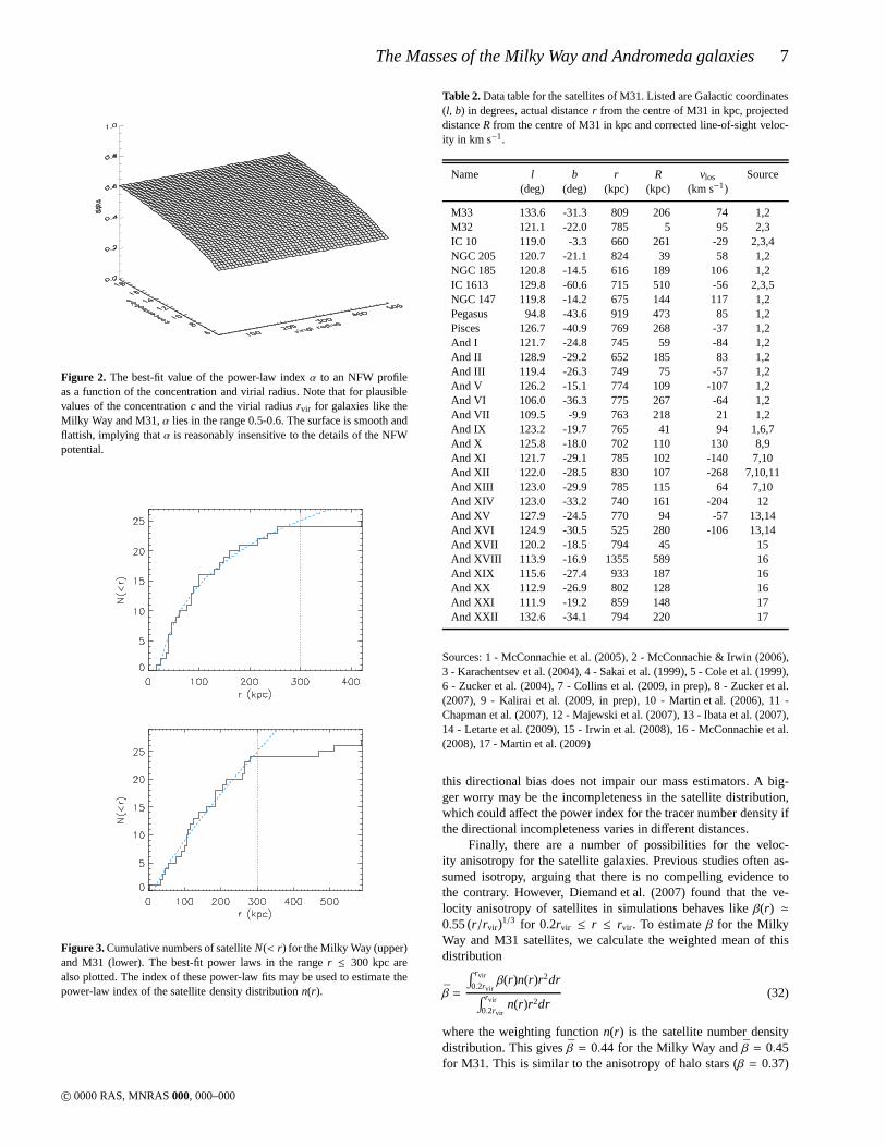
If the satellite number density distributionn(r) follows apower law with indexγ, then the number of satellites within anyradius,N(< r), also follows a power-law with index 3− γ. We fitpower-laws to the Milky Way and M31 satellite cumulative distri-butions in order to estimateγ. We restrict ourselves to the inner re-gions of the satellite distributions,r ≤ 300 kpc; beyond this range,the satellite population is likely to be seriously incomplete. Thedistributions and the best-fitting power laws are shown in Figure 3;the Milky Way data is shown in the upper panel and M31 data isshown in the lower panel. We findγ = 2.6 for the Milky Way andγ = 2.1 for M31. Note that data from the Sloan Digital Sky Survey(SDSS; York et al. 2000) has been instrumental in the identificationof many of the recently-discovered Milky Way dwarfs. The SDSScoverage includes only the region around the North GalacticCap,and, as such, the distribution of known Milky Way satellitesis con-centrated in that area of the sky. However, given our underlying as-sumption that the distribution of satellites is spherically symmetric,

c© 0000 RAS, MNRAS000, 000–000


Figure 2. The best-fit value of the power-law indexα to an NFW profileas a function of the concentration and virial radius. Note that for plausiblevalues of the concentrationc and the virial radiusrvir for galaxies like theMilky Way and M31,α lies in the range 0.5-0.6. The surface is smooth andflattish, implying thatα is reasonably insensitive to the details of the NFWpotential.

Figure 3. Cumulative numbers of satelliteN(< r) for the Milky Way (upper)and M31 (lower). The best-fit power laws in the ranger ≤ 300 kpc arealso plotted. The index of these power-law fits may be used to estimate thepower-law index of the satellite density distributionn(r).

Table 2. Data table for the satellites of M31. Listed are Galactic coordinates(l, b) in degrees, actual distancer from the centre of M31 in kpc, projecteddistanceR from the centre of M31 in kpc and corrected line-of-sight veloc-ity in km s−1.

Name l b r R vlos Source(deg) (deg) (kpc) (kpc) (km s−1)

M33 133.6 -31.3 809 206 74 1,2M32 121.1 -22.0 785 5 95 2,3IC 10 119.0 -3.3 660 261 -29 2,3,4NGC 205 120.7 -21.1 824 39 58 1,2NGC 185 120.8 -14.5 616 189 106 1,2IC 1613 129.8 -60.6 715 510 -56 2,3,5NGC 147 119.8 -14.2 675 144 117 1,2Pegasus 94.8 -43.6 919 473 85 1,2Pisces 126.7 -40.9 769 268 -37 1,2And I 121.7 -24.8 745 59 -84 1,2And II 128.9 -29.2 652 185 83 1,2And III 119.4 -26.3 749 75 -57 1,2And V 126.2 -15.1 774 109 -107 1,2And VI 106.0 -36.3 775 267 -64 1,2And VII 109.5 -9.9 763 218 21 1,2And IX 123.2 -19.7 765 41 94 1,6,7And X 125.8 -18.0 702 110 130 8,9And XI 121.7 -29.1 785 102 -140 7,10And XII 122.0 -28.5 830 107 -268 7,10,11And XIII 123.0 -29.9 785 115 64 7,10And XIV 123.0 -33.2 740 161 -204 12And XV 127.9 -24.5 770 94 -57 13,14And XVI 124.9 -30.5 525 280 -106 13,14And XVII 120.2 -18.5 794 45 15And XVIII 113.9 -16.9 1355 589 16And XIX 115.6 -27.4 933 187 16And XX 112.9 -26.9 802 128 16And XXI 111.9 -19.2 859 148 17And XXII 132.6 -34.1 794 220 17

Sources: 1 - McConnachie et al. (2005), 2 - McConnachie & Irwin (2006),3 - Karachentsev et al. (2004), 4 - Sakai et al. (1999), 5 - Coleet al. (1999),6 - Zucker et al. (2004), 7 - Collins et al. (2009, in prep), 8 - Zucker et al.(2007), 9 - Kalirai et al. (2009, in prep), 10 - Martin et al. (2006), 11 -Chapman et al. (2007), 12 - Majewski et al. (2007), 13 - Ibata et al. (2007),14 - Letarte et al. (2009), 15 - Irwin et al. (2008), 16 - McConnachie et al.(2008), 17 - Martin et al. (2009)

this directional bias does not impair our mass estimators. Abig-ger worry may be the incompleteness in the satellite distribution,which could affect the power index for the tracer number density ifthe directional incompleteness varies in different distances.

Finally, there are a number of possibilities for the veloc-ity anisotropy for the satellite galaxies. Previous studies often as-sumed isotropy, arguing that there is no compelling evidence tothe contrary. However, Diemand et al. (2007) found that the ve-locity anisotropy of satellites in simulations behaves like β(r) ≃0.55(r/rvir)

1/3 for 0.2rvir ≤ r ≤ rvir . To estimateβ for the MilkyWay and M31 satellites, we calculate the weighted mean of thisdistribution

β =

∫ rvir

0.2rvirβ(r)n(r)r2dr

∫ rvir

0.2rvirn(r)r2dr

(32)

where the weighting functionn(r) is the satellite number densitydistribution. This givesβ = 0.44 for the Milky Way andβ = 0.45for M31. This is similar to the anisotropy of halo stars (β = 0.37)

c© 0000 RAS, MNRAS000, 000–000


Figure 4. The sensitivity of the estimated mass on the anisotropy parameterβ for a satellite population withα = 0.55, β = 0 andγ = 2.7. The figureshows the mass recovered using the input values ofα andγ and varying thevalue ofβ. The functional form of the curve is easy to deduce. It is a rationalfunction ofβ for the upper panel, which uses the estimator of eqn (23), anda linear function ofβ for the lower panel, which uses eqn (16).

in simulations reported by Xue et al. (2008). Even though thesenumbers have the backing of simulations, they are somewhat sur-prising. Most of the Milky Way satellites with measured propermotions are moving on polar or tangential orbits. Using the sampleof the 7 Milky Way satellites with proper motions, we can computethe radial and tangential components of the Galactocentricvelocity.From these, the observed anisotropyβ ∼ -4.5, which favours tan-gential orbits. This is consistent with the earlier, thoughindirect,estimate of Wilkinson & Evans (1999), who foundβ ∼ -1, againfavouring tangential orbits. The origin of this discrepancy betweensimulations and data is not well understood. Perhaps there is con-siderable cosmic scatter in the anisotropy of the satellites, as it maydepend on the details of the accretion history of the host galaxy.Figure 4 plots brings both good news and bad. The upper panelshows that the mass estimates for external galaxies using the lineof sight estimator of eqn (23) are reasonably insensitive tothe pre-cise value ofβ. This make sense, as for a galaxy like M31, theline of sight velocity encodes information on both the radial andtangential velocity components referred to the M31’s centre. How-ever, in the case of the Milky Way, the situation is very different.The measured velocities provide information almost whollyon theradial component referred to the Galactic Center. In the absencesof proper motions, the velocity anisotropy is largely unconstrainedby the data. This is the classical mass-anisotropy degeneracy, andso – as the lower panel shows – there is considerable uncertainty inthe mass estimates inferred using eqn (16).

Figure 5. The fractional contribution each satellite makes to the mean massestimator for the Milky Way (top) and M31 (bottom). For both galaxies, themass budget is dominated by two satellites. For the Milky Waythese areLeo I (red, dotted) and Hercules (blue, dashed). For M31, these are AndXII (red, dotted) and And XIV (blue, dashed).

In what follows, we typically quote mass estimates for theanisotropies derived both from observationsβdata and from simu-lationsβsim, as well as for the case of isotropy (β = 0). In the ab-sence of consistent indications to the contrary, our preference is toassume isotropy and to give greatest credence to the mass estimatesobtained with this assumption.

4.2 Radial Velocity Datasets

Armed with values forα, β andγ, we now set the mass estima-tors to work. Data for the satellites of the Milky Way and M31 aregiven in Tables 1 and 2 respectively. Objects for which no line-of-sight velocity has been measured (And XVII, And XVIII, AndXIX, And XX, And XXI and And XXII) are included in the tables,but excluded from the analysis.

Using eqn (16) and recalling that the Monte Carlo simulationsgave errors of∼ 25%, we give estimates of the mass with 100,200 and 300 kpc for the Milky Way Galaxy in Table 3. Assum-ing velocity isotropy, we obtain for the mass of the Milky WayM300 = 0.9± 0.3× 1012M⊙. The cussedness of the mass-anisotropydegeneracy is well illustrated by the fact that using the observa-tionally derivedβdatagivesM300 = 3.4± 0.9× 1012M⊙, whilst usingthat from simulations givesM300 = 0.6 ± 0.2× 1012M⊙. The hugespread in mass estimates is due to the fact that the line-of-sight ve-locities for the satellites are almost entirely providing informationon the radial velocities as judged from the Galactic Centre.Thereis almost no information on the tangential motions in our dataset.However, there are other astrophysical reasons why masses higherthan∼ 2× 1012M⊙ are disfavoured.

Using eqn (23), we obtain the mass of M31 within 300 kpc asM300 = 1.4±0.4×1012M⊙. Here, though, in sharp distinction to thecase of the Milky Way, plausible changes in the velocity anisotropygenerate modest changes of the order of 10 per cent in the massestimate, as shown in Table 3. Of course, this is understandable,as the line-of-sight velocity now has information on both the radialand tangential components, albeit tangled up in the projection.

Taking the masses derived using velocity isotropy (β = 0), wenote that this work hints at the removal of a long-standing puzzle,

c© 0000 RAS, MNRAS000, 000–000


Table 3. Enclosed mass within 100, 200 and 300 kpc for the Milky Way andAndromeda galaxies. We offer three estimates: one using the anisotropy inferredfrom data (β ∼ -4.5), one assuming isotropy (β = 0) and the third with the anisotropy derived from simulations (β ∼ 0.45).

Galaxy M300 (×1011M⊙) M200 (×1011M⊙) M100 (×1011M⊙)βdata isotropic βsim βdata isotropic βsim βdata isotropic βsim

Milky Way 34.2± 9.3 9.2± 2.5 6.6± 1.8 21. 1± 5.7 5.5± 1.6 3.8± 1.0 13.9± 4.9 3.3± 1.1 2.1± 0.7... excl Leo I 25.2± 7.5 6.9± 1.8 5.0± 1.2 ... ... ... ... ... ...... excl Leo I, Her 21.1± 6.3 5.8± 1.5 4.2± 1.1 17. 5± 5.3 4.6± 1.4 3.2± 0.8 ... ... ...MW with PMs 38.6± 7.0 24.1± 5.3 22.1± 5.3 28. 3± 5.5 18.5± 4.2 17.0± 4.2 22.2± 5.0 13.8± 3.9 11.4± 3.1... excl Draco 27.1± 4.9 14.1± 3.1 12.2± 2.7 18. 1± 3.4 10.0± 2.3 8.7± 2.2 12.9± 3.1 6.9± 1.9 5.4± 1.5... excl LMC/SMC 38.8± 6.8 24.6± 5.8 21.7± 4.9 28. 3± 5.7 18.4± 4.3 16.3± 4.1 22.7± 5.6 13.9± 4.2 11.2± 3.4... excl Draco, LMC/SMC 25.9± 5.1 12.4± 2.9 10.6± 2.5 17. 0± 3.5 8.5± 2.2 7.2± 1.8 11.3± 2.9 5.4± 1.7 4.2± 1.3

M31 15.8± 3.3 14.1± 4.1 13.1± 3.8 15. 4± 4.1 12.4± 3.8 10.6± 3.5 2.6± 1.0 2.1± 1.0 1.8± 1.0... excl AndXII 12.2± 2.7 10.9± 3.1 10.1± 3.2 11. 4± 3.2 9.2± 3.1 7.9± 2.8 ... ... ...... excl AndXII, AndXIV 9.6± 2.1 8.5± 2.4 8.0± 2.4 8. 6± 2.6 6.9± 2.4 5.9± 2.2 ... ... ...M31 with PMs 15.1± 3.8 13.9± 3.5 13.1± 3.5 ... ... ... ... ... ...

namely that the kinematic data on the satellite galaxies suggestedthat M31 was less massive than the Milky Way, whereas other indi-cators (such as the total numbers of globular clusters or theampli-tude of the gas rotation curve) suggested the reverse. In fact, withthe new datasets, the ratio of the masses of M31 to the Milky Way(∼ 1.5) is close to that which would be inferred using the Tully-Fisher relationship and the assumption that the luminosityis pro-portional to the total mass (2504/2204 ≈ 1.67). If instead the radialanisotropies derived from simulations are preferred, thenthe ratiois∼ 1.98.

However, it may be imprudent to include all the satellites. Forexample, Leo I has long been known to dominate mass estimatesof the Milky Way, on account of its large distance (∼ 260 kpc) andhigh line-of-sight velocity (see e.g. Kulessa & Lynden-Bell 1992;Kochanek 1996; Wilkinson & Evans 1999). It is unclear that Leo Iis actually on a bound orbit, as opposed to a hyperbolic one. Hence,many attempts at determining the mass of the Milky Way quote es-timates both including and excluding Leo I. In fact, recent photo-metric and spectroscopic evidence presented by Sohn et al. (2007)favours the picture in which Leo I is bound on an orbit with higheccentricity (∼ 0.95) and small perigalacticon (10-15 kpc). In par-ticular, such models give good matches to the surface density andradial velocity dispersion profiles of Leo I, and imply high massestimates for the Milky Way. However, Sales et al. (2007) usingsimulations found a population of satellite galaxies on extreme or-bits ejected from haloes as a result of three-body slingshoteffects,and suggested that Leo I might be an example of such an object.So, although the present evidence favours a bound orbit, a defini-tive verdict must await the measurement of Leo I’s proper motionby theGaiasatellite, which should resolve the issue.

Given that there is one satellite that is known to inflate theMilky Way’s mass, it is interesting to investigate whether any ofthe other satellites, particularly the recent discoveries, play similarroles. The upper panel of Figure 5 shows the fractional contribu-tions each satellite makes to the Milky Way’s mass (Cv2

losrα/(GN))

– it is the total of these values that we take to be the mass esti-mate. There are two clear outliers; the outermost satellitein thisdistribution is Leo I, the less extreme satellite is Hercules. LikeLeo I, Hercules has a substantial radial velocity and a relativelylarge Galactocentric distance (∼ 130 kpc). Hercules has a highlyelongated, irregular and flattened structure (Belokurov etal. 2007;Coleman et al. 2007). This is consistent with tidal disruption dur-

ing pericentric passages on a highly eccentric orbit (e > 0.9). Thisseems good evidence that Hercules is truly bound to the MilkyWay.

We repeat the same analysis for M31 and the results are shownin the bottom panel of Figure 5. Interestingly, we see that there aretwo outliers in the distribution, namely two of the recent discover-ies, And XII and And XIV. Notice that though both objects haveasubstantial effect on M31’s mass estimate, neither are as extremeas Leo I. It is the inclusion of these two new objects in the satel-lite dataset that has augmented the mass of M31, so that it is nowsomewhat greater than that of the Milky Way.

But, this begs the question: should these satellites be included?And XIV was discovered by Majewski et al. (2007) in a survey ofthe outer M31 stellar halo. They recognized its extreme dynami-cal properties and suggested that it may either be falling into M31for the first time or that M31’s mass must be larger than hithertoestimated by virial arguments. In fact, And XIV’s lack of gasandits elongated structure suggest that ram pressure stripping and tidaleffects may have been important in its evolution. This is consistentwith And XIV being a true satellite of M31 that has already suf-fered a pericentric passage, a conclusion that could be strengthenedwith deeper imaging, which might reveal the presence of tidal tailsaround And XIV.

And XII is a still more ambiguous object – it was discoveredas a stellar overdensity by Martin et al. (2006). Spectroscopic ob-servations were subsequently taken by Chapman et al. (2007), whoconjectured that the satellite might be falling into the Local Groupfor the first time. The evidence for this is its large velocityand itslikely location behind M31. However, it remains unclear whetherthis evolutionary track is consistent with the absence of detectionof HI gas in the object. Pristine, infalling dwarfs, which have notyet experienced a pericentric passage of 50 kpc or less, should re-tain sizeable amounts of neutral HI gas, whereas Chapman et al.(2007) constrain the mass in HI to be less than 3× 103M⊙.

In light of this, we provide more mass estimates, after remov-ing possible ambiguous objects (and re-computing the parameterγwhere necessary). For the Milky Way, we exclude Leo I only andthen Leo I and Hercules. For M31, we exclude And XII only andthen And XII and And XIV. These mass estimates are also shownin Table 3. Note that, for example, the exclusion of Leo I doesnotchange the mass estimate within 100 or 200 kpc, as Leo I is out-side of this range. Similarly, And XII and And XIV lie outsideof100 kpc from the center of M31, so the mass estimates withoutthem do not change the final column of the table.

c© 0000 RAS, MNRAS000, 000–000


Figure 6. Distribution ofβ obtained from simultaneous mass and velocity anisotropy fitting. The median of each distribution is shown as a blue dashed lineand the 68 % confidence limits as cyan dotted lines. These values are also given in blue and cyan on the plot. The left panel shows the idealised case for 500tracers, the right panel the case tailored to our M31 data where only 21 tracers are used. The value ofβ used to generate the tracer population is also shown.

In the case of velocity isotropy (β = 0), it requires the excisionof both And XII and And XIV from the datasets for the mass es-timate of M31 to become comparable to or smaller than the MilkyWay. For example, the mass of M31 with And XII and And XIVboth removed is 0.85± 0.24× 1012M⊙, as compared to the mass ofthe Milky Way with Leo I retained of 0.92± 0.25× 1012M⊙. How-ever, we have argued that And XIV is most likely bound, whilstAnd XII is a more ambiguous case. In other words, the problempointed to by Evans & Wilkinson (2000) – namely that the massof M31 inferred from the kinematics of the satellites is lessthanthe mass of the Milky Way – has indeed been ameliorated by thediscovery of more fast-moving M31 satellites.

It seems particularly intriguing that such satellites exist forboth the Milky Way and M31. Wilkinson & Evans (1999) used viri-alized models to estimate that the probability that, in a sample of30 satellites, there is an object like Leo I, which changes the massestimate by a factor of a few. They found that the probabilityisminute, only∼ 0.5%. Prior expectation does not favour the exis-tence of objects like Leo I or And XII, yet in fact, both big galaxiesin the Local Group possess such satellites. The clear conclusionis that the satellites in the outer parts of these galaxies cannot allbe virialized. This is a point in favour of processes such as thoseadvocated by Sales et al. (2007) to populate such orbits.

4.3 Simultaneous Solution for Mass and Anisotropy

There is one further way in which the estimators can be set to workwith the line-of-sight velocities. When three dimensionalpositionsand projected positions are simultaneously available – as for exam-ple in the case of M31’s satellites – it is possible to use the estima-tors based on both the〈v2

losrα〉 and the〈v2

losRα〉 moments to solve

simultaneously for both the total mass and the anisotropy parame-

Table 4. Table of proper motion data for the satellites of the Milky Way andM31. Listed are equatorial proper motions in mas century−1.

Name µα cosδ µδ Source(mas/century) (mas/century)

Carina 22± 9 15± 9 1Draco 60± 40 110± 30 2Fornax 48± 5 -36± 4 3LMC/SMC 198± 5 25± 5 4Sculptor 9± 13 2± 13 5Sextans -26± 41 10± 44 6Ursa Minor -50± 17 22± 16 7M33 2.1± 0.7 2.5± 1.2 8IC10 -0.2± 0.8 2.0± 0.8 9

M31 2.1± 1.1 -1.0± 0.9 10

Sources: 1 - Piatek et al. (2003), 2 - Scholz & Irwin (1994), 3 -Piatek et al. (2007), 4 - Piatek et al. (2008), 5 - Piatek et al.(2006), 6 -Walker et al. (2008), 7 - Piatek et al. (2005), 8 - Brunthaler et al. (2007a),9 - Brunthaler et al. (2007b), 10 - van der Marel & Guhathakurta (2008),though unlike the other proper motions, this not a measurement but inferredfrom indirect evidence.

ter. There is however no guarantee that the solution forβ is in thephysical range−∞ ≤ β ≤ 1.

The success of this procedure of course rests on the accuracyof the data. The distances of the M31 satellites are determined bythe tip of the red giant branch method and have errors of±30 kpc(see e.g., McConnachie et al. 2005). If we use eqns (23) and (26),and simultaneously solve for the unknowns, we obtain

M300 = 1.5± 0.4× 1012M⊙, β = −0.55+1.1−3.2 (33)

c© 0000 RAS, MNRAS000, 000–000


Figure 7. Distribution of mass estimates as a fraction of true mass forMonteCarlo simulations using (top) 23 satellites with radial velocities, (middle) 7satellites with proper motions and (bottom) 23 satellites,7 of which haveproper motions. The standard deviation of the best fitting Gaussian is shownin the top-right hand corner of each panel. [These plots assumeβ = −4.51,as estimated from the data].

Figure 8. The fractional contribution each satellite with proper motionsmakes to the mean mass estimate for the Milky Way Galaxy. Notice theextreme effect of Draco’s proper motion.

which corresponds to mild tangential anisotropy. These aresurpris-ingly sensible answers given the distance errors.

Fig. 6 is inferred from Monte Carlo simulations and showsthe distributions of anisotropy parameters derived from simultane-ous mass and anisotropy fitting for mock datasets. Also giveninthe panels are the median and 68 per cent confidence limits fortheanisotropy parameter, in the case of 21 satellite galaxies (compara-ble to the present dataset for M31) and the case of 500 satellites.Although with 21 tracers, the errors on the anisotropy parameterare substantial, matters improve significantly with largernumbersof tracers. A dataset of 500 halo satellites (dwarf galaxies, globularclusters and planetary nebulae) is not unreasonable for a galaxy likeM31 in the near future. This raises the possibility that the methodof simultaneous fitting may prove more compelling in the future. Infact, given 500 tracers, it is reasonable to use the estimators basedon both the〈v2

losrα〉 and the〈v2

losRα〉 moments to fit simultaneously

at each distance, thus giving the run of anisotropy parameter andmass with radius.

4.4 Radial and Proper Motion Datasets

Thus far, we have used only the line of sight velocities to make massestimates. In this section, we add in the proper motions of satellites,where available. Thus, for the Milky Way galaxy, we combine re-sults from eqn (16) for satellites without proper motions and fromeqn (24) for those with proper motions, weighting each estimate bythe reciprocal of the standard deviation to give the final answer.

Proper motions, albeit with large error bars, have been mea-sured for a total of 9 of the Milky Way satellite galaxies. It seemsprudent to exclude Sagittarius, as it is in the process of merg-ing with the Milky Way. Additionally, the interacting MagellanicClouds are treated as a single system by computing the propermo-tion of their mass centroid, taking the masses of the LMC and SMCas∼ 2 × 1010M⊙ and 2× 109M⊙ respectively (Kroupa & Bastian1997). This leaves us with a set of 7 satellites with proper mo-tion data, summarized in Table 4. In most cases, errors on propermotions are large and, where multiple studies exist, the mea-surements are sometimes in disagreement. The proper motionsinferred by ground based methods are in reasonable agreementwith those derived from theHubble Space Telescope(HST) inthe cases of Fornax (Piatek et al. 2007; Walker et al. 2008), Ca-rina (Piatek et al. 2003; Walker et al. 2008) and the MagellanicClouds (Piatek et al. 2008; Costa et al. 2009). But, for Ursa Mi-nor (Scholz & Irwin 1994; Piatek et al. 2005) and for Sculptor(Piatek et al. 2006; Walker et al. 2008), agreement between differ-ent investigators is not good, and we have preferred to use the es-timates derived fromHSTdata. Nonetheless, it is important to in-clude the proper motion data, especially for mass estimatesof theMilky Way Galaxy. We use these proper motions along with dis-tance and line-of-sight velocity data to calculate full space veloci-ties for these satellites, as described in Piatek et al. (2002).

In addition, there are two satellites of M31 with measuredproper motions, namely M33 and IC 10. This astonishing feat hasexploited theVery Long Baseline Arrayto measure the positionsof water masers relative to background quasars at multiple epochs(Brunthaler et al. 2005, 2007b). Unfortunately, the technique can-not be extended to M31 itself, as it does not contain any watermasers, and so its proper motion is much less securely known.However, van der Marel & Guhathakurta (2008) reviewed the ev-idence from a number of sources – including kinematics of theM31 satellites, the motions of the satellites at the edge of the Lo-cal Group, and the constraints imposed by the tidal distortion of

c© 0000 RAS, MNRAS000, 000–000


M33’s disk – to provide a best estimate. These data are also listedin Table 4.

The Milky Way satellites are so remote that their line-of-sightvelocities in the Galactic rest frame are almost identical to theirradial velocities, as judged form the Galactic Centre. The propermotion data provide genuinely new information on the tangentialmotions and this is the only way to break the mass-anisotropyde-generacy. The same argument does not hold with equal force forM31, as the line of sight velocities incorporate contributions fromboth the radial and tangential components as reckoned from thecentre of M31. Nonetheless, it is good practice to use all thedataavailable, even though the proper motions of M33 and IC 10 withrespect to the M31 reference frame must be inferred using an esti-mate of M31’s proper motion (rather than a measurement).

For the satellites without proper motions, we use the form ofthe estimator given in eqns (16) or (23) for the Milky Way andM31 respectively; for those with proper motions, we use eqn (24).We combine results from the two estimators, weighting each esti-mate by the reciprocal of the standard deviation to give the finalanswer. To infer the standard deviation, we perform Monte Carlosimulations. So, for the case of the Milky Way, we generate mockdatasets of 25 satellites, for which only 7 have proper motions. Theerrors on radial velocities are dwarfed by the uncertainty caused bythe small number statistics and so are neglected. But, the errors onthe proper motions are not negligible and they are incorporated intothe simulations by adding a value selected at random from therange[-0.5 µ, 0.5µ], whereµ is the proper motion. The flat distributionhas been chosen as systematic errors are as important as randomGaussian error in the determination of proper motions. However,we have tested alternatives in which we use the relative observa-tional errors, or the relative observational errors multiplied by 2.5,and find that our results are robust against changes to the error law.The standard deviations of the fractional mass distribution the satel-lites with and without proper motions are separately computed, asillustrated in the panels of Figure 7. We linearly combine the massestimates, weighting with the reciprocal of the standard deviation,to give the final values reported in Table 3.

Given that the Milky Way satellites with measured proper mo-tions are moving on polar orbits, it is no surprise that the mass esti-mate of the Milky Way has now increased. Adopting the value ofβ

we estimate from the data, we findM300 = 3.9 ± 0.7× 1012M⊙ forthe Milky Way Galaxy andM300 = 1.5±0.4×1012M⊙ for M31. As-suming isotropy, we findM300 = 2.5± 0.5× 1012M⊙ for the MilkyWay Galaxy andM300 = 1.4± 0.4× 1012M⊙ for M31. Notice how-ever, the mass estimate for M31 has barely changed from the valueinferred from the full radial velocity dataset.

Again, we calculate the contribution that each satellite makesto the mass estimate to investigate whether any are dominating thefinal answer. First, this procedure guards against the possibility ofa completely rogue proper motion measurement. Second, there aresome suggestions that the Magellanic Clouds may not be bound, oreven if bound may only be on its second passage and so may notbe part of the relaxed distribution of satellite galaxies (Besla et al.2007). So, it is helpful to check that our results are not unduly sen-sitive to its inclusion. As Figure 8 shows, we find that Draco is aclear outlier and nearly doubles the Milky Way mass estimate. If weremove the Draco proper motion from the sample, we instead re-cover a massM300= 2.7± 0.5×1012M⊙ (assumingβdata) or M300=

1.4± 0.3×1012M⊙ (assuming isotropy). It is particularly concern-ing that the proper motion of Draco has such a substantial effect,because – as judged from the size of the error bars in Table 4 – it isone of the noisier measurements. By contrast, the exclusionof the

Magellanic Clouds has only a minor effect, as is evident from theresults listed in Table 3.

We have covered a number of possibilities, so it is probablyuseful for us to give our best estimates. On balance, we thinkthecase for including at least And XIV among the satellite sample forAndromeda is strong. Whilst And XII is a more ambiguous case,the lack of any HI gas suggests to us that it should also be included.Among the satellites of the Milky Way, we favour including LeoI based on the work of Sohn et al. (2007), whilst we are inclinedto discard the proper motion of Draco reported in Scholz & Irwin(1994) until corroborated. Until the discrepancy between the veloc-ity anisotropies reported in simulations and in data is explained, weprefer to use the data as our guide

So, our best estimate for the mass of the Milky Way within300 kpc is

M300 ∼ 2.7± 0.5× 1012M⊙ (34)

whilst for M31, it is

M300 ∼ 1.5± 0.4× 1012M⊙. (35)

These estimates are obtained using the combined radial velocityand proper motion datasets. The error bars only incorporatethe sta-tistical uncertainty. As we have emphasised, there are muchgreateruncertainties induced by selection of satellite members and velocityanisotropy. In particular, when these uncertainties are considered,it is not possible to decide which of the Milky Way or M31 is moremassive based on satellite kinematic data alone.

5 DISCUSSION

It is instructive to compare our results with a number of recent es-timates of the masses of the Local Group and its component galax-ies. Xue et al. (2008) extracted a sample of∼ 2400 blue horizontalbranch stars from the SDSS. These are all resident in the inner halowithin 60 kpc of the Galactic centre. This has the advantage that theBHBs are surely virialized, but the disadvantage that no inferencecan be made about the mass exterior to 60 kpc. Hence, any estimateas to the total mass is driven wholly by prior assumptions ratherthan the data. In fact, Xue et al. (2008) assumed an NFW halo witha canonical concentration holds, and then estimated the virial massof the Milky Way’s dark matter halo asM = 1.0+0.3

−0.2 × 1012M⊙,using Jeans modelling with an anisotropy parameter inferred fromnumerical simulations. This is lower than our preferred value, butin good agreement with our comparable calculations using line ofsight velocity datasets alone.

A somewhat similar calculation for M31 has been reported bySeigar et al. (2008). The mass of the baryonic material is estimatedusing a Spitzer 3.6µm image of the galaxy, together with a mass-to-light ratio gradient based on the galaxy’sB − R colour. This iscombined with an adiabatically-contracted NFW halo profileto re-produce the observed HI rotation curve data. They find a totalvirialmass of M31’s dark halo as 8.2± 0.2× 1011M⊙. This is lower thanmost of our estimates, with the exception of those based on samplesexcluding both And XII and And XIV.

Although these calculations are interesting, it is worth remark-ing that the final masses are not wholly controlled by the data. Weknow that, from Newton’s theorem, any mass distribution outsidethe limiting radius of our data has no observational effect in a spher-ical or elliptical system. To estimate the virial mass from data con-fined to the inner parts (such as BHBs or the optical disk) requiresan understanding of the structure of the pristine dark halo initially,

c© 0000 RAS, MNRAS000, 000–000


as well as how it responds to the formation of the luminous bary-onic components. It is this that controls the final answer.

Li & White (2008) used the Millennium Simulation to ex-tract mock analogues of the Local Group and calibrate the biasand error distribution of the Timing Argument estimators (seee.g., Kahn & Woltjer 1959; Raychaudhury & Lynden-Bell 1989).From this, they obtain a total mass of the two large galaxies inthe Local Group of 5.3 × 1012M⊙ with an inter-quartile range of[3.8 × 1012, 6.8 × 1012] M⊙ and a 95 % confidence lower limit of1.8×1012M⊙. Importantly, Li & White (2008) showed that the massestimate from the timing argument is both unbiased and reasonablyrobust. This is a considerable advance, as there have long been wor-ries that the gross simplification of two-body dynamics implicit inthe original formulation of the Timing Argument may undermineits conclusions.

It therefore seems reasonable to assume that the combinedmass of the Milky Way Galaxy and M31 is at least 3.8 × 1012M⊙,and perhaps more like 5.3 × 1012M⊙. The low estimates of theMilky Way and M31 masses of Xue et al. (2008) and Seigar et al.(2008) are not compatible with this, and barely compatible with Li& White’s 95 % lower limit. Using our preferred values in eqns(34)and (35), the combined mass in the Milky Way and M31 galaxiesis 4.2± 0.6× 1012M⊙. This is comparable to the 3.8× 1012M⊙ of Li& White.

Li & White (2008) also estimated a virial mass for the MilkyWay of 2.4 × 1012M⊙ with a range of [1.1 × 1012,3.1 × 1012] M⊙,based on timing arguments for Leo I. Given all the uncertainties,this is in remarkable accord with our best estimate.

6 CONCLUSIONS

We have derived a set of robust tracer mass estimators, and dis-cussed the conditions under which they converge. Given the po-sitions and velocities of a set of tracers – such as globular clus-ters, dwarf galaxies or stars – the estimators compute the enclosedmass within the outermost datapoints. The accuracy of the esti-mator has been quantified with Monte Carlo simulations. The es-timators are applicable to a wide range of problems in contem-porary astrophysics, including measuring the masses of ellipticalgalaxies, the haloes of spiral galaxies and galaxy clustersfromtracer populations. They are considerably simpler to use than dis-tribution function based methods (see e.g. Little & Tremaine 1987;Kulessa & Lynden-Bell 1992; Wilkinson & Evans 1999), and in-volve no more calculation than taking weighted averages of com-binations of the positional and kinematical data. They should findwidespread applications.

The mass estimators are applied to the satellite populations ofthe Milky Way and M31 to find the masses of both galaxies within300 kpc. These estimates are the first to make use of the recentburstof satellite discoveries around both galaxies. Both satellite popu-lations have nearly doubled in size since previous estimates weremade. We summarise our results by answering the questions; Whatare (1) the minimum, (2) the maximum and (3) the most likelymasses of the Milky Way and M31 galaxies?

(1) The mass of the Milky Way Galaxy within 300 kpc could be aslow as 0.4 ± 0.1 × 1012M⊙. This would imply that Leo I is grav-itationally unbound, contrary to the recent evidence provided byby Sohn et al. (2007). Leo I would then be either an interloperor anobject being ejected from the Milky Way by an encounter. It wouldalso require that the proper motion of Draco (Scholz & Irwin 1994)is incorrect, which is not inconceivable given the difficulty of the

measurements. It implies that the satellite galaxies are moving onradial orbits and so the velocity anisotropy is radial.

The mass of M31 within 300 kpc could plausibly be as lowas 0.8± 0.2× 1012M⊙. This would be the case if both And XII andAnd XIV are not gravitationally bound, which is possible if mecha-nisms such as those proposed by Sales et al. (2007) are ubiquitous.It would also require that the proper motion data on M33 and IC10or – perhaps more likely – the indirectly inferred proper motion ofM31 is in error. Again, such a low estimate for the mass occursonlyif the satellites are moving predominantly radially.

Although it is interesting to ask how low the masses of theMilky Way and M31 could be, it does produce a mystery in thecontext of the Timing Argument, which typically yields largercombined masses. It is possible that some of the mass of the Lo-cal Group is unassociated with the large galaxies. Althoughnotthe conventional picture, this is probably not ruled out andtherehave been suggestions that∼ 1012M⊙ may be present in the Lo-cal Group in the form of baryons in the warm-hot intergalacticmedium (Nicastro et al. 2003). There are few constraints on thepossible existence of dark matter smeared out through the LocalGroup, and unassociated with the large galaxies. However, the clus-tering of the dwarf galaxies around the Milky Way and M31 doessuggest that the gravity of the dark matter is centered on thepromi-nent galaxies.

(2) The largest mass estimate we obtained for the Milky WayGalaxy is 3.9± 0.7× 1012M⊙. This extreme values is driven by theassumption of tangential anisotropy for the satellites, sothat themeasured line of sight velocities also imply substantial tangentialmotions as well. The estimate assumes all the satellites includingLeo I to be bound, and the anomalously high proper motion mea-surement of Draco to be valid.

Note that the present data allow considerably more scope toincrease the mass of the Milky Way Galaxy than M31. Our largestmass estimate for M31 is a much more modest 1.6± 0.4× 1012M⊙,which occurs when we analyse the whole sample incorporatingAnd XII and And XIV and assume tangentially anisotropic velocitydistributions.

The current concensus is that the two galaxies are of a roughlysimilar mass, with M31 probably the slightly more massive ofthetwo. This though is inferred from indirect properties, suchas thenumbers of globular clusters, which correlates with total mass al-beit with scatter, or the amplitude of the inner gas rotationcurve.The stellar halo of M31 is certainly more massive than that oftheMilky Way, although this may not be a good guide to the dark halo.Of course, it could be that the current concensus is wrong, and thatthe Milky Way halo is more massive than that of Andromeda. Thereis also some indirect evidence in favour of this – for example, thetypical sizes of the M31 dwarf spheroidals are large than those ofthe Milky Way, which is explicable if the Milky Way halo is denser.However, it does not seem reasonable to postulate that the mass ofthe Milky Way is substantially larger than that of M31. Hence, thevery large estimate of 3.9 ± 0.7 × 1012M⊙ is best understood as amanifestation of the degeneracy in the problem of mass estimationwith only primarily radial velocity data.

(3) Our preferred estimates come from accepting Leo I, And XIIand And XIV as bound satellites, whilst discarding the Dracoproper motion as inaccurate. This gives an estimate for the mass ofthe Milky Way within 300 kpc as 2.7± 0.5× 1012M⊙ and for M31as 1.5± 0.4× 1012M⊙, assuming the anisotropy implied by the data(β ≈ −4.5). The error bars are just the statistical uncertainty and donot incorporate the uncertainty in anisotropy or sample member-

c© 0000 RAS, MNRAS000, 000–000


ship. In view of this, it is not possible to decide which of theMilkyWay galaxy or M31 is the more massive based on the kinematicdata alone.

These values for the masses are attractive for a number ofreasons. First, the mass ratio between the Milky Way and M31 isof roughly of order unity, which accords with a number of otherlines of evidence. Second, the values allow most of the dark matterin the Local Group implied by the Timing Argument to be clus-tered around the two most luminous galaxies. Third, they arewithinthe range found for cosmologically motivated models of the MilkyWay and M31 (Li & White 2008).

We prefer to assume the anisotropy implied by the admittedlyscanty data on the proper motions of the satellites. However, forcompleteness, we quickly sketch the effects of dropping this as-sumption. If the velocity distribution is isotropic, or even radiallyanisotropic as suggested by the simulations, then the mass of theMilky Way becomes 1.4± 0.3× 1012M⊙ or 1.2± 0.3× 1012M⊙ re-spectively. Similarly for M31, the values are 1.4 ± 0.4 × 1012M⊙(isotropy) or 1.3± 0.4× 1012M⊙ (radially anisotropic).

The greatest sources of uncertainty on the masses remain therole ofpossibly anomalous satellites like Leo I and the velocity anisotropyof the satellite populations. There is reason to be optimistic, astheGaia satellite will provide proper motion data on all the dwarfgalaxies that surround the Milky Way and M31, as well as manyhundreds of thousands of halo stars. The analysis that we have car-ried out here indicates that proper motions are important ifwe wishto increase the accuracy of our estimates, as well as understand thedynamical nature of objects like Leo I. While we are not yet ableto exploit the proper motions,Gaiawill allow us to do so.

ACKNOWLEDGMENTS

NWE thanks Simon White for a number of insightful discussionson the matter of scale-free estimators. LLW thanks the Scienceand Technology Facilities Council of the United Kingdom forastudentship. Work by JHA is in part supported by the ChineseAcademy of Sciences Fellowships for Young International Sci-entists (Grant No.:2009Y2AJ7). JHA also acknowledges supportfrom the Dark Cosmology Centre funded by the Danish NationalResearch Foundation (Danmarks Grundforskningsfond). Thepaperwas considerably improved following the comments of an anony-mous referee.

REFERENCES

Armandroff T. E., Olszewski E. W., Pryor C., 1995, AJ, 110, 2131Bahcall J. N., Tremaine S., 1981, ApJ, 244, 805Bellazzini M., Ferraro F. R., Origlia L., Pancino E., MonacoL., Oliva E.,

2002, AJ, 124, 3222Bellazzini M., Gennari N., Ferraro F. R., 2005, MNRAS, 360, 185Bellazzini M., Gennari N., Ferraro F. R., Sollima A., 2004, MNRAS, 354,

708Belokurov V. et al., 2008, ApJ, 686, L83Belokurov V. et al., 2009, MNRAS, p. 903Belokurov V. et al., 2007, ApJ, 654, 897Belokurov V. et al., 2006, ApJ, 647, L111Besla G., Kallivayalil N., Hernquist L., Robertson B., Cox T. J., van der

Marel R. P., Alcock C., 2007, ApJ, 668, 949Binney J., Tremaine S., 1987, Galactic dynamics.Princeton, NJ, Princeton

University Press, 1987Braun R., 1991, ApJ, 372, 54

Brunthaler A., Reid M. J., Falcke H., Greenhill L. J., HenkelC., 2005, Sci-ence, 307, 1440

Brunthaler A., Reid M. J., Falcke H., Henkel C., Menten K. M.,2007a,arXiv:0708.1704

Brunthaler A., Reid M. J., Falcke H., Henkel C., Menten K. M.,2007b,A&A, 462, 101

Chapman S. C. et al., 2007, ApJ, 662, L79Cioni M.-R. L., van der Marel R. P., Loup C., Habing H. J., 2000, A&A,

359, 601Cole A. A. et al., 1999, AJ, 118, 1657Coleman M. G. et al., 2007, ApJ, 668, L43Costa E., Mendez R. A., Pedreros M. H., Moyano M., Gallart C., Noel N.,

Baume G., Carraro G., 2009, AJ, 137, 4339Crain R. A. et al., 2009, MNRAS, 399, 1773Dehnen W., Binney J. J., 1998, MNRAS, 298, 387Diemand J., Kuhlen M., Madau P., 2007, ApJ, 667, 859Evans N. W., Hafner R. M., de Zeeuw P. T., 1997, MNRAS, 286, 315Evans N. W., Wilkinson M. I., 2000, MNRAS, 316, 929Evans N. W., Wilkinson M. I., Guhathakurta P., Grebel E. K., Vogt S. S.,

2000, ApJ, 540, L9Evans N. W., Wilkinson M. I., Perrett K. M., Bridges T. J., 2003, ApJ, 583,

752Fellhauer M. et al., 2006, ApJ, 651, 167Freedman W. L. et al., 2001, ApJ, 553, 47Geha M., Willman B., Simon J. D., Strigari L. E., Kirby E. N., Law D. R.,

Strader J., 2009, ApJ, 692, 1464Gottesman S. T., Hunter J. H., Boonyasait V., 2002, MNRAS, 337, 34Harris J., Zaritsky D., 2006, AJ, 131, 2514Heisler J., Tremaine S., Bahcall J. N., 1985, ApJ, 298, 8Helmi A., 2004, ApJ, 610, L97Ibata R., Martin N. F., Irwin M., Chapman S., Ferguson A. M. N., Lewis

G. F., McConnachie A. W., 2007, ApJ, 671, 1591Ibata R. A., Wyse R. F. G., Gilmore G., Irwin M. J., Suntzeff N. B., 1997,

AJ, 113, 634Irwin M. J. et al., 2007, ApJ, 656, L13Irwin M. J., Ferguson A. M. N., Huxor A. P., Tanvir N. R., IbataR. A.,

Lewis G. F., 2008, ApJ, 676, L17Johnston K. V., Law D. R., Majewski S. R., 2005, ApJ, 619, 800Kahn F. D., Woltjer L., 1959, ApJ, 130, 705Kaluzny J., Kubiak M., Szymanski M., Udalski A., KrzeminskiW., Mateo

M., 1995, A&AS, 112, 407Karachentsev I. D., Karachentseva V. E., Huchtmeier W. K., Makarov D. I.,

2004, AJ, 127, 2031Karachentsev I. D., Kashibadze O. G., Makarov D. I., Tully R.B., 2009,

MNRAS, 393, 1265Klypin A., Zhao H., Somerville R. S., 2002, ApJ, 573, 597Koch A., Kleyna J. T., Wilkinson M. I., Grebel E. K., Gilmore G. F., Evans

N. W., Wyse R. F. G., Harbeck D. R., 2007, AJ, 134, 566Koch A., Wilkinson M. I., Kleyna J. T., Gilmore G. F., Grebel E. K., Mackey

A. D., Evans N. W., Wyse R. F. G., 2007, ApJ, 657, 241Koch A. et al., 2009, ApJ, 690, 453Kochanek C. S., 1996, ApJ, 457, 228Kroupa P., Bastian U., 1997, New Astronomy, 2, 77Kulessa A. S., Lynden-Bell D., 1992, MNRAS, 255, 105Law D. R., Majewski S. R., Johnston K. V., 2009, ApJ, 703, L67Letarte B. et al., 2009, arXiv:0901.0820Li Y., White S. D. M., 2008, MNRAS, 384, 1459Little B., Tremaine S., 1987, ApJ, 320, 493Lynden-Bell D., Frenk C. S., 1981, The Observatory, 101, 200Majewski S. R. et al., 2007, ApJ, 670, L9Martin N. F., de Jong J. T. A., Rix H.-W., 2008, ApJ, 684, 1075Martin N. F., Ibata R. A., Chapman S. C., Irwin M., Lewis G. F.,2007,

MNRAS, 380, 281Martin N. F., Ibata R. A., Irwin M. J., Chapman S., Lewis G. F.,Ferguson

A. M. N., Tanvir N., McConnachie A. W., 2006, MNRAS, 371, 1983Martin N. F. et al., 2009, arXiv:0909.0399Mateo M. L., 1998, ARA&A, 36, 435McConnachie A. W. et al., 2008, ApJ, 688, 1009

c© 0000 RAS, MNRAS000, 000–000

http://arxiv.org/abs/0708.1704




McConnachie A. W., Irwin M. J., 2006, MNRAS, 365, 902McConnachie A. W., Irwin M. J., Ferguson A. M. N., Ibata R. A.,Lewis

G. F., Tanvir N., 2005, MNRAS, 356, 979Navarro J. F., Frenk C. S., White S. D. M., 1996, ApJ, 462, 563Nicastro F. et al., 2003, Nature, 421, 719Piatek S., Pryor C., Bristow P., Olszewski E. W., Harris H. C., Mateo M.,

Minniti D., Tinney C. G., 2005, AJ, 130, 95Piatek S., Pryor C., Bristow P., Olszewski E. W., Harris H. C., Mateo M.,

Minniti D., Tinney C. G., 2006, AJ, 131, 1445Piatek S., Pryor C., Bristow P., Olszewski E. W., Harris H. C., Mateo M.,

Minniti D., Tinney C. G., 2007, AJ, 133, 818Piatek S., Pryor C., Olszewski E. W., 2008, AJ, 135, 1024Piatek S. et al., 2002, AJ, 124, 3198Piatek S., Pryor C., Olszewski E. W., Harris H. C., Mateo M., Minniti D.,

Tinney C. G., 2003, AJ, 126, 2346Queloz D., Dubath P., Pasquini L., 1995, A&A, 300, 31Raychaudhury S., Lynden-Bell D., 1989, MNRAS, 240, 195Rohlfs K., Kreitschmann J., 1988, A&A, 201, 51Sakai S., Madore B. F., Freedman W. L., 1999, ApJ, 511, 671Sales L. V., Navarro J. F., Abadi M. G., Steinmetz M., 2007, MNRAS, 379,

1475Saviane I., Held E. V., Bertelli G., 2000, A&A, 355, 56Scholz R.-D., Irwin M. J., 1994, in MacGillivray H. T., ed., IAU Sympo-

sium Vol. 161, Astronomy from Wide-Field Imaging. p. 535Seigar M. S., Barth A. J., Bullock J. S., 2008, MNRAS, 389, 1911Simon J. D., Geha M., 2007, ApJ, 670, 313Sohn S. T. et al., 2007, ApJ, 663, 960van der Marel R. P., Alves D. R., Hardy E., Suntzeff N. B., 2002, AJ, 124,

2639van der Marel R. P., Guhathakurta P., 2008, ApJ, 678, 187Walker M. G., Mateo M., Olszewski E. W., 2008, ApJ, 688, L75Walker M. G., Mateo M., Olszewski E. W., Bernstein R., Wang X.,

Woodroofe M., 2006, AJ, 131, 2114Walker M. G., Mateo M., Olszewski E. W., Pal J. K., Sen B., Woodroofe

M., 2006, ApJ, 642, L41White S. D. M., 1981, MNRAS, 195, 1037Wilkinson M. I., Evans N. W., 1999, MNRAS, 310, 645Xue X. X. et al., 2008, ApJ, 684, 1143York D. G. et al., 2000, AJ, 120, 1579Zucker D. B. et al., 2006, ApJ, 650, L41Zucker D. B. et al., 2006, ApJ, 643, L103Zucker D. B. et al., 2004, ApJ, 612, L121Zucker D. B. et al., 2007, ApJ, 659, L21

c© 0000 RAS, MNRAS000, 000–000

Documents

The Masses of the Milky Way and Andromeda Galaxies · The Masses of the Milky Way and Andromeda galaxies 3 parameter, in which σt is the tangential velocity dispersion. Now, β→