The Mathematica Journal Simulation of Evolutionary ... · The Mathematica® Journal Simulation of Evolutionary Dynamics in Finite Populations Bernhard Voelkl In finite populations,

The Mathematica® Journal

Simulation of Evolutionary Dynamics in Finite PopulationsBernhard Voelkl

In finite populations, evolutionary dynamics can no longer be described by deterministic differential equations, but require a stochastic formulation [1]. We show how Mathematica can be used to both simulate and visualize evolutionary processes in limited populations. The Moran process is introduced as the basic stochastic model of an evolutionary process in finite populations. This model is extended to mixed populations with relative fitness differences. We combine population ecology with game theoretic ideas, simulating evolutionary games in well-mixed and structured populations.

‡ The Moran ProcessThe Moran process is a simple stochastic model to study selection in finite populations[2]. We consider a population of constant size with two types of individuals, type 1 andtype 0. At each time step a single individual is allowed to reproduce a clone of the sametype. Furthermore, to keep the population size constant, one individual must die. TheMoran process is a birth-death update process. Individuals for reproduction and elimina-tion are chosen randomly. If both random choices fall on the same individual, the individ-ual will be replaced by its own identical offspring and the population remains unchanged.The variable i denotes the number of type 1 individuals in the population of size n. Thenumber of type 0 individuals is therefore n- i. The Moran process is defined on the statespace i = 0, …, n. The probability of choosing a type 1 individual is given by i ê n and theprobability of choosing a type 0 individual is Hn- iL ê n.

The Mathematica Journal 13 © 2011 Wolfram Media, Inc.

If a type 0 individual is chosen for reproduction and a type 1 individual for elimination, idecreases by one. If a type 1 individual is chosen for reproduction and a type 0 individualfor elimination, i increases by one. In all other cases the populations of types 1 and 0remain unchanged. The according probabilities for these events are given by:

(1)pi,i-1 = iHn- iL ë n2 ,pi,i+1 = iHn- iL ë n2,pi,i = 1- pi,i-1 - pi,i+1.

As p0, 1 = 0 and pn, n-1 = 0, p0,0 = 1 and pn, n = 1. The states i = 0 and i = n are thereforeabsorbing states: when the process has reached such a state it cannot change anymore.Although both types of individuals reproduce at the same rate, one type will alwaysreplace the other. Given no time constraints, the coexistence of both types is impossible.The probability that a population with i type 1 individuals will end up in state i = n isgiven by xi = i ê n.

· Simulation of a Moran Process

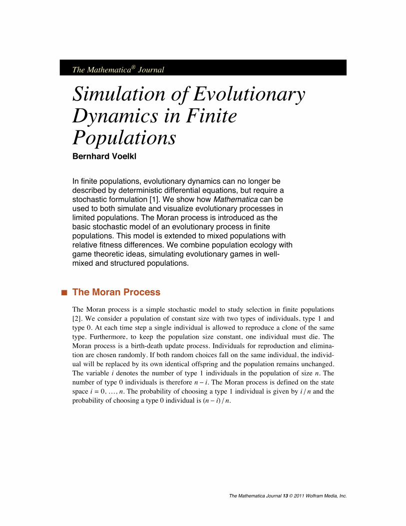
To visualize evolutionary dynamics, we represent populations as graphs where eachvertex represents an individual. This requires the package Combinatorica.The function initial@n, iD constructs a list of length n that represents the initialpopulation with i individuals of type 1 and n- i individuals of type 0.The function update@popD randomly selects two elements 8repro, elim< of thelist pop and replaces the value of elim (the individual chosen for elimination) by thevalue of repro (the individual chosen for reproduction).The function moran@n, iD starts with an initial condition of i type 1 individuals andn- i type 0 individuals. In each round, one individual is chosen for reproduction and onefor elimination. This update process is repeated until the population reaches one of thetwo absorbing states.

The function showpop@popD plots a graph without edges where pop is taken as a list ofvertex weights. The VertexRenderingFunction is used to color the vertices accord-ing to their type as represented by their vertex weights.

Now we simulate the Moran process for a population size of n = 40 individuals and i = 15type 1 individuals in the initial condition. The Manipulate function lets us see theevolution of the population. The Manipulate will work immediately without the needto evaluate it.

2 Bernhard Voelkl


Manipulate@showpop@evolutionPuTD,88u, 1<, 1, Dynamic@Length@evolutionDD, 1,Appearance Ø "Labeled"<,

AutorunSequencing Ø 81<,SynchronousInitialization Ø False,Initialization ß H

QuietüGet@"Combinatorica`"D;

initial@n_, i_D := Join@Table@1, 8i<D, Table@0, 8n - i<DD;

update@pop_ListD := Module@8repro, elim<,8repro, elim< = RandomInteger@81, Length@popD<, 2D;ReplacePart@pop, elim Ø popPreproTDD;

moran@n_, i_D := NestWhileList@update, initial@n, iD,n > Total@ÒD > 0 &D;

showpop@pop_D := Module@8g<,g = Combinatorica`SetVertexWeights@

Combinatorica`CompleteGraph@Length@popDD, popD;GraphPlot@g, EdgeRenderingFunction Ø None,VertexRenderingFunction ØH8If@Combinatorica`GetVertexWeights@gDPÒ2T ã 0,

Hue@0, 0.8, 0.7D, [email protected], 0.8, 0.7DD,[email protected], Point@ÒD< &L, ImageSize Ø 280DD;

evolution = moran@40, 15D;

If@u > Length@evolutionD, u = Length@evolutionDDLD

Simulation of Evolutionary Dynamics in Finite Populations 3


u 1

‡ The Moran Process with Relative FitnessNow we consider the case when the two types, 1 and 0, have different fitness. Fitness deter-mines the rate at which they reproduce. If we set the fitness of type 0 to 1 and the fitnessof type 1 to r, then the probability that type 1 is chosen for reproduction is given byp1 = r i ê Hr i+ n- iL and the probability that type 0 is chosen is given byp0 = Hn- iL ê Hr i+ n- iL. The probabilities for being chosen for elimination remain un-changed. The fixation probability for i type 1 individuals is given by:

(2)xi =1- 1 ê ri

1- 1 ê rn.

Because the probability of being chosen for reproduction depends now on the continuousvariable r, the simulation is modified. In updateRel@pop, rD we evaluate the numberof type 1 individuals that is equivalent to the total of the list pop. Thereafter we evaluatereprod, the probability with which a type 1 individual is chosen for reproduction. Fi-nally we randomly select one element of list pop and replace it by 1 with probabilityreprod and by 0 with probability 1 - reprod. The function moranRel@n, i, rD simulates a Moran process in a mixed population ofsize n with i individuals with relative fitness r and n- i individuals with relative fitness 1.

4 Bernhard Voelkl


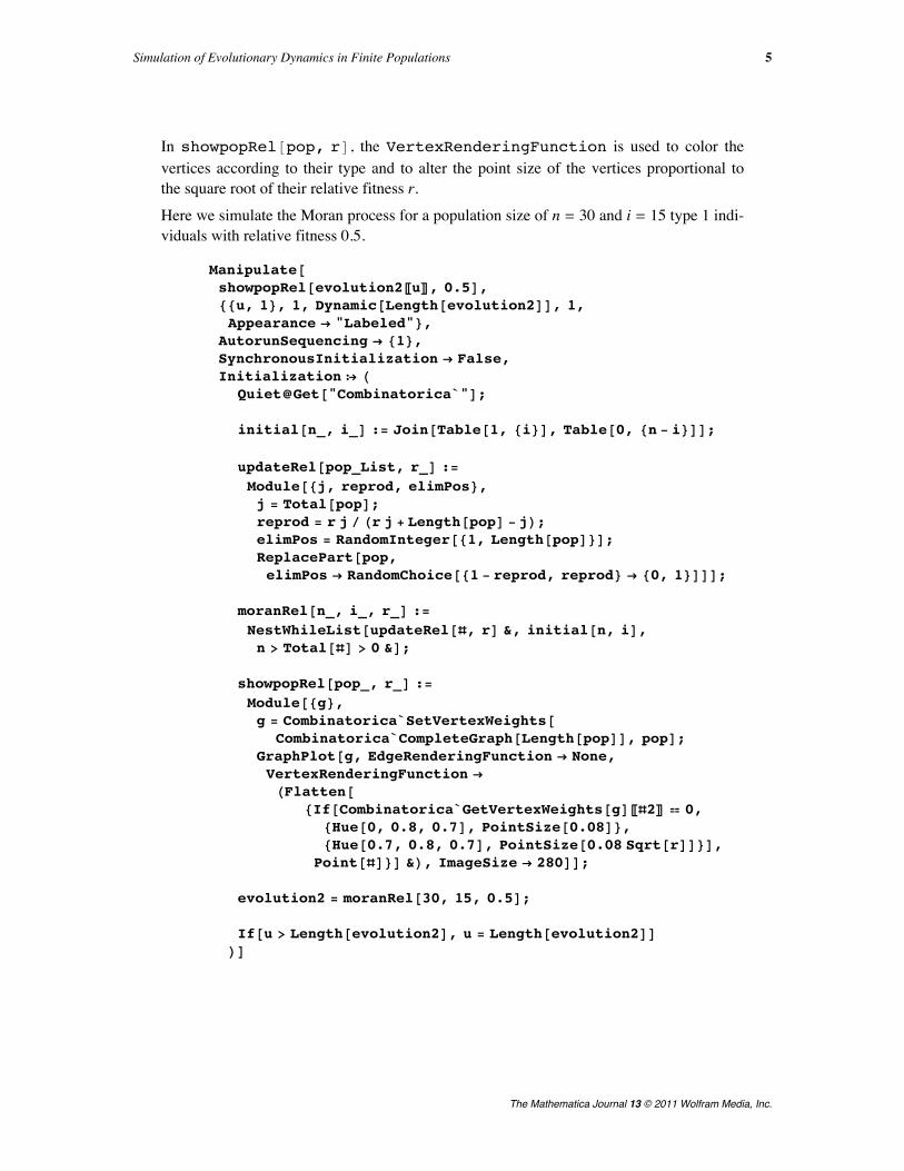
In showpopRel@pop, rD, the VertexRenderingFunction is used to color thevertices according to their type and to alter the point size of the vertices proportional tothe square root of their relative fitness r. Here we simulate the Moran process for a population size of n = 30 and i = 15 type 1 indi-viduals with relative fitness 0.5.

Manipulate@showpopRel@evolution2PuT, 0.5D,88u, 1<, 1, Dynamic@Length@evolution2DD, 1,Appearance Ø "Labeled"<,



initial@n_, i_D := Join@Table@1, 8i<D, Table@0, 8n - i<DD;

updateRel@pop_List, r_D :=Module@8j, reprod, elimPos<,j = Total@popD;reprod = r j ê Hr j + Length@popD - jL;elimPos = RandomInteger@81, Length@popD<D;ReplacePart@pop,elimPos Ø RandomChoice@81 - reprod, reprod< Ø 80, 1<DDD;

moranRel@n_, i_, r_D :=NestWhileList@updateRel@Ò, rD &, initial@n, iD,n > Total@ÒD > 0 &D;

showpopRel@pop_, r_D :=Module@8g<,g = Combinatorica`SetVertexWeights@

Combinatorica`CompleteGraph@Length@popDD, popD;GraphPlot@g, EdgeRenderingFunction Ø None,VertexRenderingFunction ØHFlatten@

8If@Combinatorica`GetVertexWeights@gDPÒ2T ã 0,8Hue@0, 0.8, 0.7D, [email protected]<,[email protected], 0.8, 0.7D, [email protected] Sqrt@rDD<D,

Point@ÒD<D &L, ImageSize Ø 280DD;

evolution2 = moranRel@30, 15, 0.5D;

If@u > Length@evolution2D, u = Length@evolution2DDLD



u 1

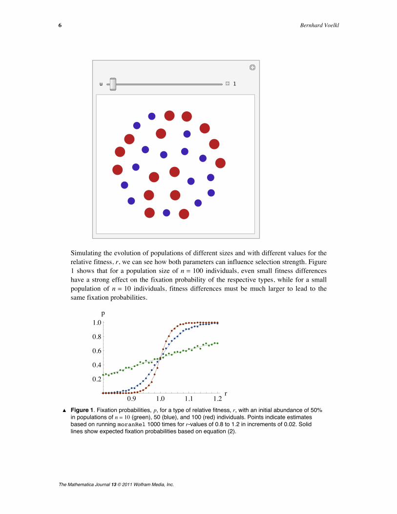
Simulating the evolution of populations of different sizes and with different values for therelative fitness, r, we can see how both parameters can influence selection strength. Figure1 shows that for a population size of n = 100 individuals, even small fitness differenceshave a strong effect on the fixation probability of the respective types, while for a smallpopulation of n = 10 individuals, fitness differences must be much larger to lead to thesame fixation probabilities.

0.9 1.0 1.1 1.2r

0.2

0.4

0.6

0.8

1.0p

Ú Figure 1. Fixation probabilities, p, for a type of relative fitness, r, with an initial abundance of 50% in populations of n = 10 (green), 50 (blue), and 100 (red) individuals. Points indicate estimates based on running moranRel 1000 times for r-values of 0.8 to 1.2 in increments of 0.02. Solid lines show expected fixation probabilities based on equation (2).

6 Bernhard Voelkl


‡ Evolutionary GamesWe consider a population with two types of individuals, where individuals interact witheach other at regular rates. Whenever two individuals interact with each other, theyreceive payoffs from this interaction according to the payoff matrix:

(3)1 0

10

a bc d

As the probability that two individuals of specified type interact depends on the relativefrequencies of the types given by i for type 1 and n- i for type 0, the expected payoffs fortype 1 and type 0 are:

(4)

FH1L i =a Hi- 1L+ b Hn- 1L

n- 1,

FH0L i =c i+ d Hn- i- 1L

n- 1.

Payoffs contribute to the fitness of the individuals by

(5)fH1L i = 1-w+w FH1L i,fH0L i = 1-w+w FH0L i,

where ri = fH1L i ê fH0L i. The parameter w is a measure for the strength of selection. If w = 1,fitness is completely determined by the payoff; if w = 0, fitness is independent of the pay-off. When studying evolutionary processes, biologists usually assume that lifetime fitnessof an individual is determined by many variables, thus any single gene will only have aweak effect on selection. A selective strength w between 0.01 and 0.05 is often suggestedto study evolution under weak selection.

To start the simulation we choose a population size n and define population as anempty list. The number of type 1 individuals, i, is chosen randomly from the interval@1, n- 1D. We create a list strategies of length n and set i randomly chosen elementsto 1 while the remaining elements are 0. (The randomization of the positions is not neces-sary right now, as it will not influence the outcome, but it will become important later on.)This list represents our population and is equivalent to the list pop in the previous section.For our model of selection we introduce a death-birth update process. This means that inevery round a randomly chosen individual will be eliminated and the vacated space willbe taken over by a new individual. The probability that this new individual will be of type1 is proportional to the overall fitness of the type 1 individuals in the neighborhood ofelim. Fitness is evaluated after elimination, thus the effective population size neequals n- 1.



The function fitness@strategies, elim, nD takes the list strategies,deletes the entry at position elim, and evaluates the relative fitness of type 1 according toequations (4) and (5). In this case the payoffs a- d are chosen so that the game representsa prisoner’s dilemma and we set the selection strength w to 0.05.

As in the previous section, we repeat the update process with updateGame until one ofthe two absorbing states is reached. In each round we randomly choose one individual forelimination. Thereafter we request a random number. If this random number is below thelimit evaluated by the function fitness, the eliminated individual is replaced by a type1 individual, otherwise by a type 0 individual.In showGame@r, strategiesD, VertexRenderingFunction is used to colorthe vertices according to their type as indicated by the vertex weight list strategiesand to alter the point size of the vertices in proportion to their relative fitness, where i isthe number of type 1 individuals in strategies and r ê i is the relative fitness for type 1.The Manipulate function lets us see the evolution of the population.

Manipulate@showGame üü populationPuT,88u, 1<, 1, Dynamic@Length@populationDD, 1,Appearance Ø "Labeled"<,



updateGame@pop_, n_D :=Module@8elim<, elim = RandomInteger@81, n<D;If@Random@D § fitness@popP2T, elim, nD,ReplacePart@pop, 82, elim< Ø 1D,ReplacePart@pop, 82, elim< Ø 0DD

D;

fitness@strategies_, elim_, n_D :=Module@8i, f1, f0, a, b, c, d, w<,i = Total@Delete@strategies, elimDD;f1 = 1 - w + w Ha i Hi - 1L + b i Hn - 1 - iLL ê Hn - 1L;f0 =1 - w + w Hc i Hn - 1 - iL + d Hn - 1 - iL Hn - 2 - iLL ê Hn - 1L;

f1 ê Hf1 + f0L êê. 8a Ø 5, b Ø 0, c Ø 3, d Ø 1, w Ø 0.05<D;

population = Module@8n = 16, strategies, r<,strategies = ReplacePart@Table@0, 8n<D,

Partition@RandomSample@Range@nD,RandomInteger@81, n - 1<DD, 1D Ø 1D;

r = fitness@strategies, RandomInteger@81, n<D, nD;NestWhileList@updateGame@Ò, nD &, 8r, strategies<,Total@Ò@@2DDD > 0 && Total@Ò@@2DDD < n &D

D;

8 Bernhard Voelkl


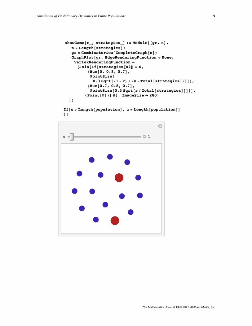
showGame@r_, strategies_D := Module@8gr, n<,n = Length@strategiesD;gr = Combinatorica`CompleteGraph@nD;GraphPlot@gr, EdgeRenderingFunction Ø None,VertexRenderingFunction ØHJoin@If@strategiesPÒ2T ã 0,

8Hue@0, 0.8, 0.7D,[email protected] Sqrt@H1 - rL ê Hn - Total@strategiesDLDD<,

[email protected], 0.8, 0.7D,[email protected] Sqrt@r ê Total@strategiesDDD<D,

8Point@ÒD<D &L, ImageSize Ø 280DD;

If@u > Length@populationD, u = Length@populationDDLD

u 1



‡ Evolutionary Games in Structured PopulationsSo far we have considered the case of well-mixed populations. That means that each indi-vidual interacts with all other individuals equally often. While this is a convenient assump-tion for modeling, anthropologists studying human organizations and biologists studyinganimal social behavior have repeatedly emphasized the fact that human and animal soci-eties are rarely well-mixed, but structured; that is, individuals usually interact only with asmall subset—a neighborhood—of the population [3, 4]. We can incorporate informationabout the structure of a population by assigning weights to the edges of the graph, wherethe edge weight is proportional to the probability that these two individuals interact witheach other [5].We study the evolution of cooperation in a small, heterogeneous population. Individualscan be either of type COOP (cooperator) or DEF (defector). When two cooperating individ-uals interact, each individual gains a benefit b from the mutual cooperative act, but alsohas to pay some costs c. If a cooperator interacts with a defector, the cooperator has to paythe costs c, but the defector gets the benefit b without paying any costs. If two defectorsmeet they get nothing, but they also have no costs. This leads to the payoff matrix

(6)Coop Def

CoopDef

b- c -cb 0

· Simulation of Games in Structured Populations

As an example we take the sociomatrix of a group of nine chimpanzees (Pantroglodytes) [6]. Entries in am represent frequencies of directed grooming actions withindyads of apes.As in the previous section, we assume a death-birth update process. In each round arandomly chosen individual is eliminated, but now only the neighborhood of this indi-vidual—that is, those individuals that interacted with the eliminated individual—competefor the vacated space [7]. The likelihood that a vacated space is filled with a type COOPindividual is proportional to the fitness of its COOP neighbors and their interactionstrength with the vacated space. The fitness of the neighbors is derived from the payoffsthese individuals gain from interactions with their neighbors.

The function probcoop evaluates the probability with which the eliminated individual atposition elim will be replaced by an individual of type COOP. First we calculatebenefits, the benefits that individuals in the neighborhood of elim receive from the in-teractions with their neighbors. Thereafter we calculate costs, the costs that individualsin the neighborhood of elim have to pay. The list nhstrat gives the strategies of theneighbors of elim, where 1 stands for a type COOP individual and 0 for a type DEF indi-vidual; benefitsCOOP sums up the benefits of only those individuals in the neighbor-hood of elim that are of type COOP, while benefitsDEF is the sum of benefits for theDEF individuals in the neighborhood of elim. Equivalently we calculate the costs forCOOP elim costsCOOPhave no costs. The variables nCOOP and nDEF give the numbers of cooperators and defec-tors in the neighborhood of elim. The relative fitness of COOP is evaluated according toequations (4) and (5). By setting c to 1, we need only one parameter value: the b ê c ratio,which characterizes the payoff matrix. As in the previous example, we assume weak selec-tion and set the selection strength w to 0.05.

10 Bernhard Voelkl


The function probcoop evaluates the probability with which the eliminated individual atposition elim will be replaced by an individual of type COOP. First we calculatebenefits, the benefits that individuals in the neighborhood of elim receive from the in-teractions with their neighbors. Thereafter we calculate costs, the costs that individualsin the neighborhood of elim have to pay. The list nhstrat gives the strategies of theneighbors of elim, where 1 stands for a type COOP individual and 0 for a type DEF indi-vidual; benefitsCOOP sums up the benefits of only those individuals in the neighbor-hood of elim that are of type COOP, while benefitsDEF is the sum of benefits for the

COOP individuals in the neighborhood of elim as costsCOOP. Type DEF individualshave no costs. The variables nCOOP and nDEF give the numbers of cooperators and defec-tors in the neighborhood of elim. The relative fitness of COOP is evaluated according toequations (4) and (5). By setting c to 1, we need only one parameter value: the b ê c ratio,which characterizes the payoff matrix. As in the previous example, we assume weak selec-tion and set the selection strength w to 0.05.To visualize evolutionary dynamics in the population, we introduce the function allfit,which gives the relative fitness for all individuals in the population. This function is notnecessary to simulate the evolutionary process, because in each round all that is needed isthe local information of the neighborhood around the eliminated individual. Especially forlarge and weakly connected populations, allfit performs a lot of superfluous compu-tations. We include allfit only for visualization purposes, but not when repeating thesimulation many times to estimate fixation probabilities. Here we simulate the evolution of a population with a population structure given by the ad-jacency matrix sociomatrix. Entries in the adjacency matrix are frequencies of dyadicinteractions per round; neigborhood is a list of length n, where the ith element is a listgiving the neighborhood of individual i. The initial number of type COOP individuals,initialcooperators, is chosen randomly from the interval @1, n- 1D and values of1 for type COOP and 0 for type DEF are randomly allocated to the population liststrategies. Strategies are updated until the population reaches an absorbing state, asdescribed in the previous section. At each round we attach a list with two elements tostructuredPopulation, containing a list with the square root of the relative fitnessfor all individuals and a list with vertex weights, denoting the individuals’ type.

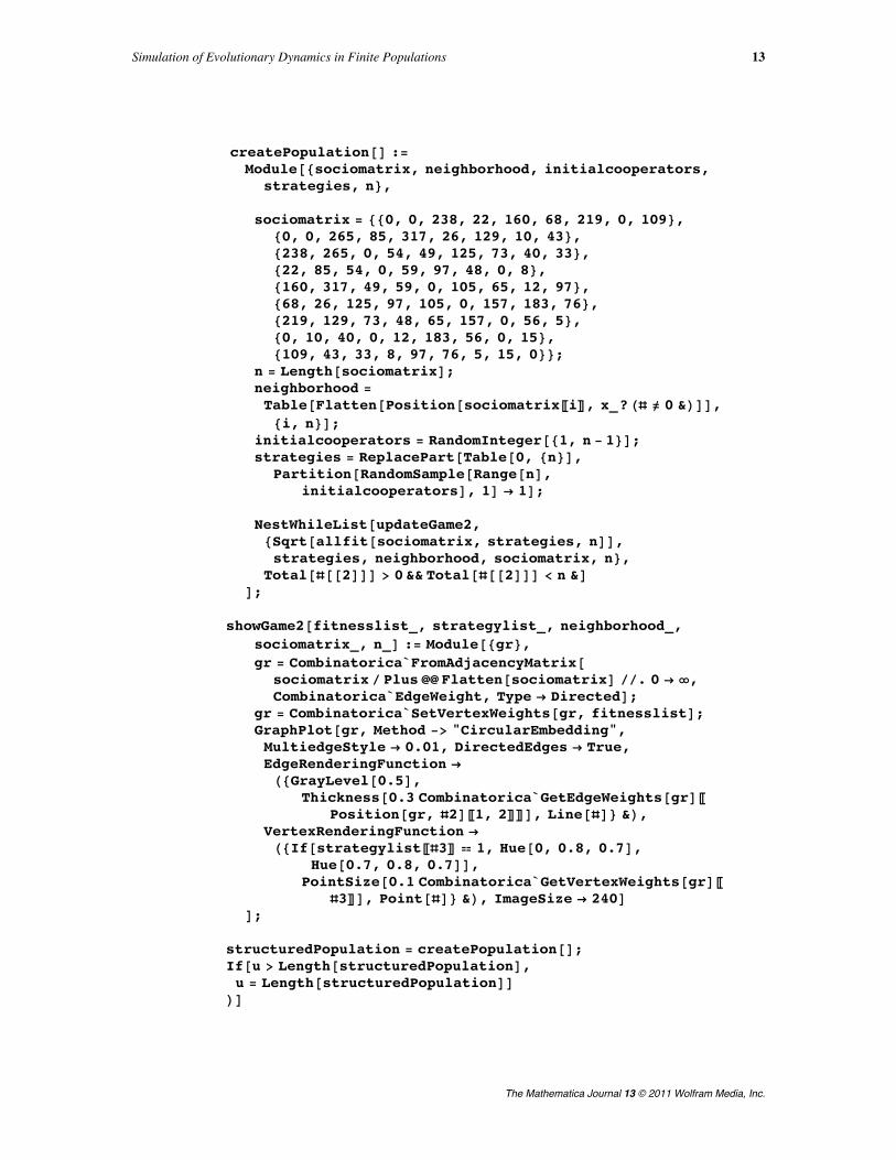
In showGame2 we use "CircularEmbedding" as the plot method, because this isthe most common visualization in the social sciences for groups of small size. TheEdgeRenderingFunction is used to visualize the strength of connections betweenthe individuals: the thickness of the line is proportional to the edge weight in the adja-cency matrix am.Here is a visualization of the evolution of a mixed, heterogeneous population of coop-erators and defectors. Defectors are indicated by red vertices; cooperators are coloredblue. Interaction frequencies are indicated by the thickness of the connecting lines.



Manipulate@showGame2 üü structuredPopulationPuT,88u, 1<, 1, Dynamic@Length@structuredPopulationDD,1, Appearance Ø "Labeled"<,



probcoop@elim_, strategies_, neighborhood_,sociomatrix_, n_D :=

Module@8benefits, costs, nhstrat, benefitsCOOP,benefitsDEF, costsCOOP, nCOOP, nDEF, fCOOP, fDEF,c, b, w<,

benefits = Apply@Plus,Table@strategies, 8Length@neighborhoodPelimTD<DTranspose@sociomatrixDPneighborhoodPelimTT , 2D;

costs = Apply@Plus, sociomatrixPneighborhoodPelimTT,2D;

nhstrat = strategiesPneighborhoodPelimTT;benefitsCOOP = Total@benefits nhstratD;benefitsDEF = Total@benefitsD - benefitsCOOP;costsCOOP = Total@costs nhstratD;nCOOP = Total@nhstratD;nDEF = Length@nhstratD - nCOOP;fCOOP = nCOOP H1 - wL + w HbenefitsCOOP b - costsCOOP cL;fDEF = nDEF H1 - wL + w benefitsDEF b;fCOOP ê HfCOOP + fDEFL ê. 8c Ø 1, b Ø 10, w -> 0.05<

D;

allfit@sociomatrix_, strategies_, n_D := Module@8w, b<,H1 - wL +

wHb Total@sociomatrix Transpose@Table@strategies,

8n<DDD - Total@Transpose@sociomatrixDDL êTotal@Flatten@sociomatrixDD êê. 8w Ø 0.05, b Ø 40<

D;

updateGame2@pop_ListD :=Module@8elim, strategies = popP2T, neighborhood = popP3T,

sociomatrix = popP4T, n = popP5T<,elim = RandomInteger@81, n<D;If@Random@D § probcoop@elim, strategies,

neighborhood, sociomatrix, nD,ReplacePart@pop, 82, elim< Ø 1D,ReplacePart@pop, 82, elim< Ø 0DD

D;

12 Bernhard Voelkl


createPopulation@D :=Module@8sociomatrix, neighborhood, initialcooperators,

strategies, n<,

sociomatrix = 880, 0, 238, 22, 160, 68, 219, 0, 109<,80, 0, 265, 85, 317, 26, 129, 10, 43<,8238, 265, 0, 54, 49, 125, 73, 40, 33<,822, 85, 54, 0, 59, 97, 48, 0, 8<,8160, 317, 49, 59, 0, 105, 65, 12, 97<,868, 26, 125, 97, 105, 0, 157, 183, 76<,8219, 129, 73, 48, 65, 157, 0, 56, 5<,80, 10, 40, 0, 12, 183, 56, 0, 15<,8109, 43, 33, 8, 97, 76, 5, 15, 0<<;

n = Length@sociomatrixD;neighborhood =Table@Flatten@Position@sociomatrixPiT, x_?HÒ ¹≠ 0 &LDD,8i, n<D;

initialcooperators = RandomInteger@81, n - 1<D;strategies = ReplacePart@Table@0, 8n<D,

Partition@RandomSample@Range@nD,initialcooperatorsD, 1D Ø 1D;

NestWhileList@updateGame2,8Sqrt@allfit@sociomatrix, strategies, nDD,strategies, neighborhood, sociomatrix, n<,

Total@Ò@@2DDD > 0 && Total@Ò@@2DDD < n &DD;

showGame2@fitnesslist_, strategylist_, neighborhood_,sociomatrix_, n_D := Module@8gr<,gr = Combinatorica`FromAdjacencyMatrix@

sociomatrix ê Plus üü Flatten@sociomatrixD êê. 0 Ø ¶,Combinatorica`EdgeWeight, Type Ø DirectedD;

gr = Combinatorica`SetVertexWeights@gr, fitnesslistD;GraphPlot@gr, Method -> "CircularEmbedding",MultiedgeStyle Ø 0.01, DirectedEdges Ø True,EdgeRenderingFunction Ø[email protected],

[email protected] Combinatorica`GetEdgeWeights@grDPPosition@gr, Ò2DP1, 2TTD, Line@ÒD< &L,

VertexRenderingFunction ØH8If@strategylistPÒ3T ã 1, Hue@0, 0.8, 0.7D,

[email protected], 0.8, 0.7DD,[email protected] Combinatorica`GetVertexWeights@grDP

Ò3TD, Point@ÒD< &L, ImageSize Ø 240DD;

structuredPopulation = createPopulation@D;If@u > Length@structuredPopulationD,u = Length@structuredPopulationDD

LD



u 1

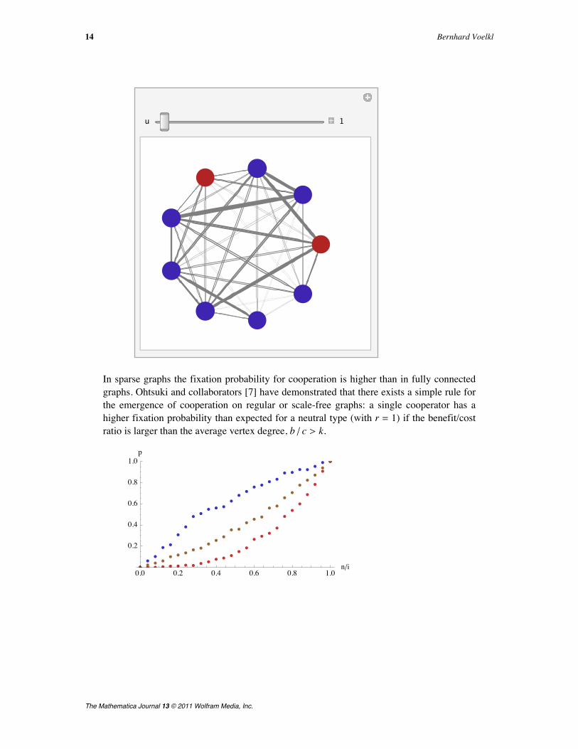
In sparse graphs the fixation probability for cooperation is higher than in fully connectedgraphs. Ohtsuki and collaborators [7] have demonstrated that there exists a simple rule forthe emergence of cooperation on regular or scale-free graphs: a single cooperator has ahigher fixation probability than expected for a neutral type (with r = 1) if the benefit/costratio is larger than the average vertex degree, b ê c > k.

0.0 0.2 0.4 0.6 0.8 1.0nêi

0.2

0.4

0.6

0.8

1.0p

14 Bernhard Voelkl


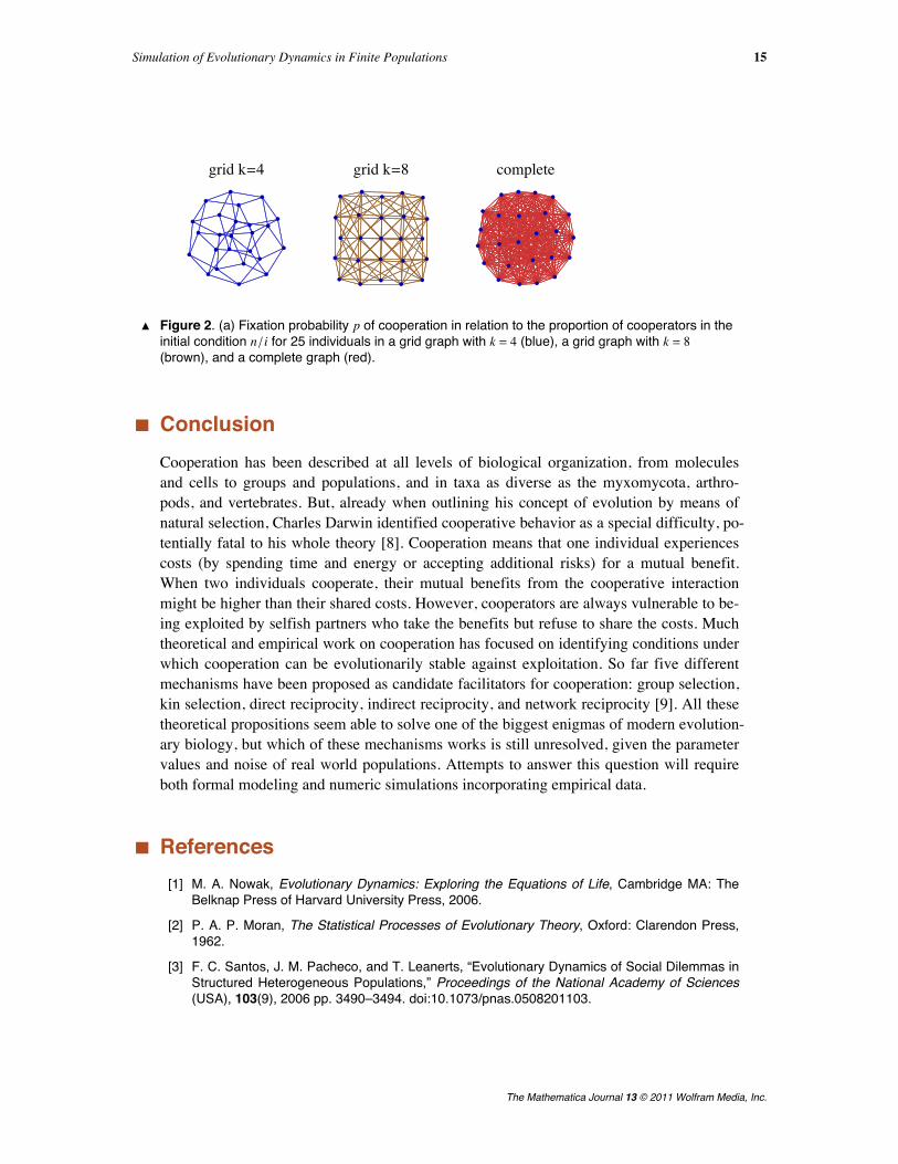
grid k=4 grid k=8 complete

Ú Figure 2. (a) Fixation probability p of cooperation in relation to the proportion of cooperators in the initial condition n ê i for 25 individuals in a grid graph with k = 4 (blue), a grid graph with k = 8 (brown), and a complete graph (red).

‡ ConclusionCooperation has been described at all levels of biological organization, from moleculesand cells to groups and populations, and in taxa as diverse as the myxomycota, arthro-pods, and vertebrates. But, already when outlining his concept of evolution by means ofnatural selection, Charles Darwin identified cooperative behavior as a special difficulty, po-tentially fatal to his whole theory [8]. Cooperation means that one individual experiencescosts (by spending time and energy or accepting additional risks) for a mutual benefit.When two individuals cooperate, their mutual benefits from the cooperative interactionmight be higher than their shared costs. However, cooperators are always vulnerable to be-ing exploited by selfish partners who take the benefits but refuse to share the costs. Muchtheoretical and empirical work on cooperation has focused on identifying conditions underwhich cooperation can be evolutionarily stable against exploitation. So far five differentmechanisms have been proposed as candidate facilitators for cooperation: group selection,kin selection, direct reciprocity, indirect reciprocity, and network reciprocity [9]. All thesetheoretical propositions seem able to solve one of the biggest enigmas of modern evolution-ary biology, but which of these mechanisms works is still unresolved, given the parametervalues and noise of real world populations. Attempts to answer this question will requireboth formal modeling and numeric simulations incorporating empirical data.

‡ References[1] M. A. Nowak, Evolutionary Dynamics: Exploring the Equations of Life, Cambridge MA: The

Belknap Press of Harvard University Press, 2006.

[2] P. A. P. Moran, The Statistical Processes of Evolutionary Theory, Oxford: Clarendon Press,1962.

[3] F. C. Santos, J. M. Pacheco, and T. Leanerts, “Evolutionary Dynamics of Social Dilemmas inStructured Heterogeneous Populations,” Proceedings of the National Academy of Sciences(USA), 103(9), 2006 pp. 3490–3494. doi:10.1073/pnas.0508201103.



[4] R. Axelrod, The Evolution of Cooperation, New York: Basic Books, 1984.

[5] B. Voelkl and R. Noë, “The Influence of Social Structure on the Propagation of Social Informa-tion in Artificial Primate Groups: A Graph-Based Simulation Approach,” Journal of Theoreti-cal Biology, 252(1), 2008 pp. 77–86. doi:10.1016/j.jtbi.2008.02.002.

[6] T. Nishida and K. Hosaka, “Coalition Strategies among Adult Male Chimpanzees of theMahale Mountains, Tanzania,” in Great Ape Societies (W. C. McGrew, L. F. Marchant, andT. Nishida, eds.), Cambridge: Cambridge University Press, 1996 pp. 114-134.

[7] H. Ohtsuki, C. Hauert, E. Lieberman, and M. A. Nowak, “A Simple Rule for the Evolution ofCooperation on Graphs and Social Networks,” Nature, 441, 2006 pp. 502–505. doi:10.1038/nature04605.

[8] C. Darwin, On the Origin of Species by Means of Natural Selection, London: J. Murray, 1859.

[9] M. A. Nowak, “Five Rules for the Evolution of Cooperation,” Science, 314, 2006pp. 1560–1563. doi:10.1126/science.1133755.

B. Voelkl, “Simulation of Evolutionary Dynamics in Finite Populations,” The Mathematica Journal, 2011. dx.doi.org/doi:10.3888/tmj.13–8.

‡ AcknowledgmentsI want to thank one anonymous reviewer for improving the program. This research hasreceived funding from the European Community’s Sixth Framework Programme(FP6/2002-2006) under contract n. 28696.

About the Author

Bernhard Voelkl started his career at the Centre National pour la Recherche Scientifique(CNRS) in Strasbourg at the Département Ecologie, Physiologie et Ethologie and is now aresearch fellow at the Center for Integrative Life Sciences in Berlin. As part of the re-search initiative GEBACO, “Towards the Genetic Basis of Cooperation,” he investigatedthe preconditions necessary for the evolution of cooperative behavior in animals. He usesMathematica for formal modeling, simulation studies, and statistical data analysis.Bernhard VoelklCenter for Integrative Life Sciences andInstitute for Theoretical Biology, Humboldt UniversityInvalidenstrasse 43, 10115 Berlin, [email protected]

16 Bernhard Voelkl


Documents

The Mathematica Journal Simulation of Evolutionary ... · The Mathematica® Journal Simulation of Evolutionary Dynamics in Finite Populations Bernhard Voelkl In finite populations,