The mathematical shell model underlying general …web.mit.edu/kjb/www/...Model_Underlying_General_Shell_Elements.pdfTitle: The mathematical shell model underlying general shell elements

INTERNATIONAL JOURNAL FOR NUMERICAL METHODS IN ENGINEERINGInt. J. Numer. Meth. Engng. 2000; 48:289–313

The mathematical shell model underlyinggeneral shell elements

Dominique Chapelle1;∗;† and Klaus-J�urgen Bathe2

1INRIA-Rocquencourt - B.P. 105 - 78153 Le Chesnay Cedex, France2Massachusetts Institute of Technology, Cambridge MA 02139, U.S.A.

SUMMARY

We show that although no actual mathematical shell model is explicitly used in ‘general shell element’ formu-lations, we can identify an implicit shell model underlying these �nite element procedures. This ‘underlyingmodel’ compares well with classical shell models since it displays the same asymptotic behaviours—when thethickness of the shell becomes very small—as, for example, the Naghdi model. Moreover, we substantiate theconnection between general shell element procedures and this underlying model by mathematically provinga convergence result from the �nite element solution to the solution of the model. Copyright ? 2000 JohnWiley & Sons, Ltd.

KEY WORDS: shell model; �nite element discretization; degenerated solid; asymptotic behaviour

1. INTRODUCTION

Since the early development of practical �nite element analysis procedures, a primary objectivewas to analyse complex shell structures [1–4]. In today’s practice, of course, shell structures areabundantly solved in many industries, including the automotive, aircraft and civil engineeringenvironments. However, although shell analyses are widely conducted, the quest for improvedanalysis procedures continues. To formulate shell �nite element discretizations, in essence, threedi�erent approaches can be followed [1–4].In the �rst approach, the shell behaviour is seen as a superposition of membrane and plate

bending actions. Finite elements are constructed by simply combining plate bending and planestress sti�ness matrices. The resulting shell elements, however, are of low performance in accuracybecause curvature e�ects are not included and the plate bending and membrane behaviour is onlycoupled at the nodal points. Much more e�ective �nite element shell analysis procedures are nowavailable.

∗Correspondence to: Dominique Chapelle, INRIA-Rocquencourt, B.P.105 - 78153 Le Chesnay Cedex, France†E-mail: [email protected]

Received 20 December 1998Copyright ? 2000 John Wiley & Sons, Ltd. Revised 24 October 1999

290 D. CHAPELLE AND K. J. BATHE

The second approach is based on using a speci�c shell theory and discretizing the correspondingvariational formulation. If the shell theory contains high-order derivatives, the �nite element dis-cretization requires corresponding nodal point variables beyond the usual nodal point displacementsand rotations. This requirement results in di�culties when more complex shell structures, that forexample include beam sti�eners, need be modelled. Another disadvantage of such an approach isthat if the shell theory is only applicable to certain shell geometries or analysis conditions, the�nite element formulation is, of course, subject to the same restrictions.In practice, a very general �nite element formulation that can be used for the analysis of virtually

any thin or moderately thick shell and in linear or non-linear analysis conditions is most attractive.The basis of such a formulation is provided by the approach of degenerating the three-dimensionalcontinuum to shell behaviour. In this approach, the mid-surface of the three-dimensional continuumis identi�ed and the basic assumptions are that �bres straight and normal to the mid-surface priorto the deformation remain straight during the deformation, and that the stress normal to the shellmid-surface is zero throughout the shell motion. With these assumptions, the construction of adisplacement-based �nite element discretization is straightforward. While this formulation is onlydirectly e�ective in very restrictive cases [2; 5], the formulation does provide the basis for mixed�nite element methods which are e�ective for general shell analyses [1; 2; 6; 7]. Speci�cally, thecomplete range of membrane and bending-dominated shell structures can be solved with thesemethods.In order to reach more e�ective shell �nite element discretization procedures, it is paramount

to perform thorough mathematical analyses of the discretization schemes. If the �nite elementmethod has been derived based upon a speci�c shell theory, clearly, the mathematical analysis isconcerned with the issues of consistency, stability and convergence measured using that theory.However, in the general approach described above, the shell �nite element analysis procedureis obtained directly from three-dimensional discretization subject to the kinematic and stress as-sumptions mentioned, without the use of a speci�c shell theory. Since the shell theory is notknown, a complete mathematical analysis is di�cult to perform and a comparison with other shellmathematical models cannot be directly achieved.The objective of this paper is to identify the two-dimensional mathematical shell model under-

lying the general three-dimensional shell analysis approach, to analyse this mathematical model,to compare the model with other well-known shell models, and �nally give convergence resultsof the displacement-based �nite element discretization scheme to the solution of the model. Themain results were already announced by the authors in Reference [8], and are now fully developedand substantiated in the present paper.The paper is organized in the following way. In Section 2, we give some de�nitions and notation

regarding the shell geometry and deformations. Then in Section 3, we derive ‘the underlying two-dimensional mathematical model’ of the general three-dimensional shell analysis approach. Thisderivation is followed in Section 4 by mathematical analyses of the model, speci�cally, with respectto membrane and bending-dominated behaviours, and with respect to the asymptotic behaviour asthe thickness of the shell domain becomes very small. In particular, we conclude that the underlyingtwo-dimensional shell model displays the same asymptotic behaviour as the Naghdi shell model. InSection 5, we then show that the general three-dimensional shell element procedure converges tothe solution of the underlying two-dimensional model as the mesh is re�ned. Finally, in Section 6,we present our conclusions regarding this work.

Copyright ? 2000 John Wiley & Sons, Ltd. Int. J. Numer. Meth. Engng. 2000; 48:289–313

THE MATHEMATICAL SHELL MODEL UNDERLYING GENERAL SHELL ELEMENTS 291

2. GEOMETRY AND NOTATION

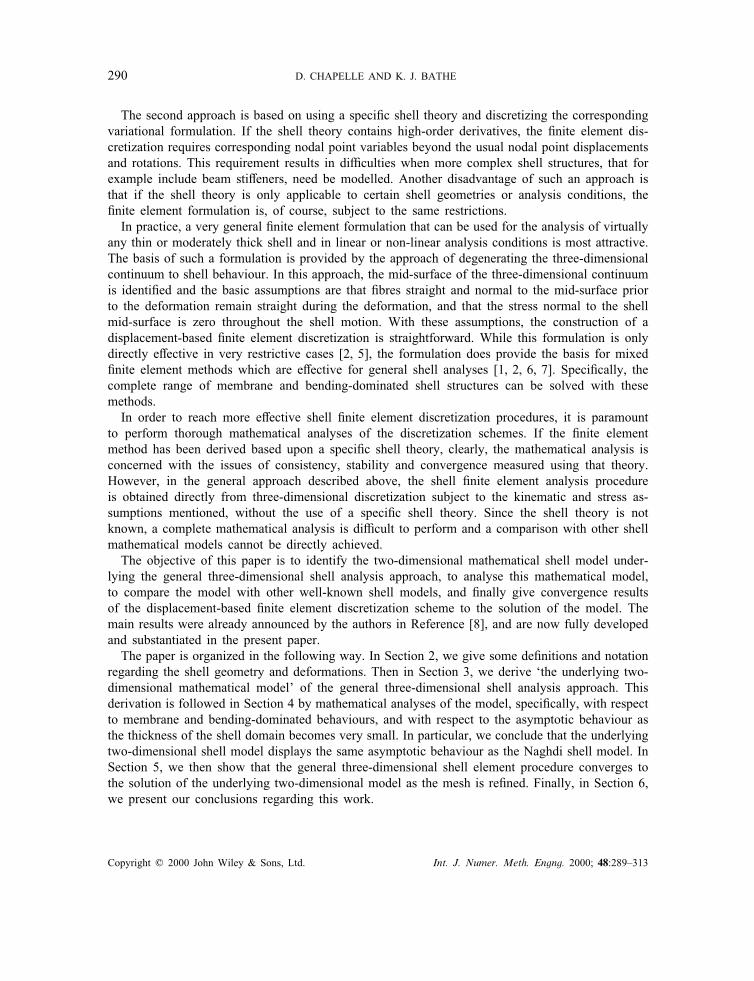
In what follows, we assume that the shell mid-surface, S, can be de�ned by a single chart M,which is a one-to-one smooth mapping from � into R3, where denotes an open domain of R2called ‘reference domain’ and thus S = M( �), see Figure 1 ( � denotes the closure of , i.e. theunion of and its boundary @). We now brie y recall the classical de�nitions and notation ofdi�erential geometry that we need for our purposes, see References [3; 9] for more details. We usethe Einstein convention on the summation of repeated indices, with the values of indices rangingin {1; 2} for Greek symbols and in {1; 2; 3} for Roman symbols. Let the covariant base vectorsof the tangential plane be de�ned by

a�def=@M(�1; �2)@��

with the contravariant base vectors (of the tangential plane) given by

a� · a� = ��where � denotes the Kronecker symbol. The unit normal vector is

a3 =a1 × a2

‖a1 × a2‖The �rst fundamental form of the surface is given by

a��def= a� · a�

or alternatively in contravariant form by

a�� def= a� · a�

The second fundamental form is de�ned by

b��def= a3 · a�;�

and the third fundamental form by

c��def= b��b��

Figure 1. De�nition of the mid-surface by a chart.



where we recall that b��def= a��b��. The following symbol appears in surface measures:

a def= ‖a1 × a2‖2 = a11a22 − (a12)2

and indeed we denote

dS def=√a d�1 d�2

The covariant di�erentiation on the mid-surface is denoted by a vertical bar (like in ‘v�|�’, seeReference [9]).The geometry of the shell is de�ned by its mid-surface and a parameter representing the thick-

ness of the three-dimensional medium lying around this surface. For simplicity of discussion wehenceforth consider shells of constant thickness, denoted by t. We de�ne the t-dependent domain

�tdef= ×]− t=2; t=2[

The geometry of the shell can then be described by the chart �, the mapping from ��t into R3de�ned by

�(�1; �2; �3) = M(�1; �2) + �3a3(�1; �2)

This parametrization de�nes a system of curvilinear co-ordinates. We can therefore introduce thethree-dimensional covariant base vectors

gidef=@�@�i

which immediately gives {g� = (�� − �3b��)a�g3 = a3

(1)

From this we can obtain the expression of the components of the three-dimensional metric tensorg�� = g� · g� = a�� − 2�3b�� + �23c��g�3 = g� · g3 = 0g33 = g3 · g3 = 1

(2)

The contravariant three-dimensional base vectors are de�ned by

gi · g j = �jihence {

g� · g� = ��g3 = a3

The de�nition of the twice-contravariant components of the metric tensor

gij def= gi · g j



gives, in particular, {g�3 = 0

g33 = 1(3)

Finally, the volume measure is expressed as

dV def=√g d�1 d�2 d�3

with

g def= [(g1 × g2) · g3]2 = a(1− 2H�3 + K�23)2

where H and K , respectively, denote the mean and Gaussian curvature of the surface (i.e. themean and the product, respectively, of the principal curvatures). We note here that the mapping� is well de�ned (hence so is the system of curvilinear co-ordinates) provided that the expression1− 2H�3 + K�23 is always strictly positive. This is clearly equivalent to requiring that

t¡2 inf(�1 ;�2)∈ �

|Rmin(�1; �2)| (4)

where Rmin(�1; �2) is the radius of curvature of smallest modulus of the surface at point M(�1; �2).We henceforth suppose that condition (4) is satis�ed.

3. DERIVATION OF THE ‘UNDERLYING 2D-MODEL’

General shell element procedures are inferred from three-dimensional formulations using two basicassumptions [1; 2; 4]:

A-1. The displacements considered are such that, at nodes, the material line normal to themid-surface in the original con�guration remains straight and unstretched during the de-formations (kinematical assumption).

A-2. The stresses in the direction normal to the mid-surface are assumed to be zero.

Of course, in practice, using assumption A-1, interpolation is employed between nodal points and,when enforcing assumption A-2, the normal direction used (at the numerical integration points)is given by the interpolation of the nodal normal vectors, see Section 5 for more details on theinterpolation.We henceforth consider an isotropic linear elastic material and we use a constitutive law inferred

from assumption A-2. The three-dimensional (3D) variational formulation reads

A(3D)(U;V) = F (3D)(V); ∀V (5)

The bilinear form A(3D) denotes the virtual work of internal forces. Using the curvilinear coordinatesystem, it can be written

A(3D)(U;V) def=∫�t[C��e��(U)e��(V) + D��e�3(U)e�3(V)] dV



where the eij’s denote the components of the linearized elastic strains and

C�� def=E

2(1 + �)

(g��g�� + g��g�� +

2�1− �g

��g��)

D�� def=2E1 + �

g��

Note that the e33 component of the strain tensors does not appear because of assumption A-2.The linear form F (3D) represents the virtual work of external forces and reads

F (3D)(V) def=∫�tF ·V dV

where F denotes the applied body forces.Equation (5) characterizes the solution of this 3D-elasticity problem for a body that is contained

within the same geometrical bounds as the shell that we want to consider. The displacementsU and V above are general 3D displacement vectors de�ned over the domain �t (they must,of course, satisfy some boundary conditions). Clearly, a general shell element procedure does notreally approximate the solution of the 3D problem, i.e. we do not expect that, when h (a parametercharacteristic of the mesh size) tends to zero, the solution of the �nite element procedure convergesto the solution of Equation (5). Instead, a good candidate problem for the limit of the �nite elementsolution is obtained by enforcing the kinematical assumption stated in assumption A-1 above inthe whole domain (and not only at nodes). We therefore introduce in Equation (5) the assumptionthat U and V have the special form

U(�1; �2; �3) = u(�1; �2) + �3��(�1; �2)a�(�1; �2) (6)

V(�1; �2; �3) = v(�1; �2) + �3��(�1; �2)a�(�1; �2) (7)

The quantities �� and �� are the covariant components of the �rst-order tensors X and W. They arede�ned in the tangent plane and correspond to the rotations of �bres normal to the mid-surface inthe original con�guration. We get the modi�ed variational formulation

A(u; X; v; W) = F(v; W); ∀(v; W) (8)

where A and F are directly inferred from A(3D) and F (3D) by setting

A(u; X; v; W) def= A(3D)(u + �3��a�; v + �3��a�)

F(v; W) def= F (3D)(v + �3��a�)

Although the integrals involved in A and F are three-dimensional, Equation (8) characterizes atwo-dimensional (2D) problem since the variational unknowns and test functions are de�ned onthe mid-surface only. We call this problem the underlying 2D shell model. Indeed, the dependenceon the �3-variable of all the terms under the integral signs can be made fully explicit. In particular,



we have

e��(v + �3��a�) = ��(v) + �3��(v; W)− �23��(W) (9)

e�3(v + �3��a�) = ��(v; W) (10)

where

��(v)def= 1

2 (v�|� + v�|�)− b��v3

��(v; W)def= 1

2 (��|� + ��|� − b��v�|� − b��v�|�) + c��v3

��(W)def= 1

2 (b��|� + b

��|�)

��(v; W)def= 1

2 (�� + v3;� + b��v�)

Note that the terms ��, �� and �� are, respectively, the components of the classical membrane,bending and shear strain tensors that appear in the Naghdi shell model [10]. Also, the unknownsinvolved in the underlying model are the same—namely, a displacement vector and a rotationtensor—as in the Naghdi model. However, the underlying model is clearly di�erent from theNaghdi model, and it is also di�erent from shell models obtained by truncating Taylor expansionsof the three-dimensional formulation (see, e.g., Reference [11]).

4. ANALYSIS OF THE UNDERLYING MODEL

We �rst need to recast Problem (8) in a rigorous mathematical context. We suppose that the shellis fully clamped on a part of its lateral boundary given by �(�0 × [−t=2; t=2]) where �0 is a partof @. We de�ne the space of admissible ‘displacements’ by

Udef= {(v; W)∈ [H 1()]3 × [H 1()]2 | v|�0 ≡ 0; W|�0 ≡ 0}

Then the following proposition shows that Problem (8) is well-posed on U (see the appendix forthe proof).

Proposition 4.1. Suppose F∈L2(�t). There exists a unique (u; X) in U such that Equation (8)is satis�ed for any (v; W) in U. Furthermore, we have

‖u; X‖16C‖F‖0 (11)

We now want to perform the asymptotic analysis of the underlying model, i.e. the analysisof the behaviour of the solution of Problem (8) when the thickness parameter t becomes verysmall (and in the limit approaches zero). To that purpose, we need to make some assumptionson the loading. In particular, the applied body force must be scaled by some power of t in orderfor the solution of the problem to remain both bounded and non-vanishing when t tends to zero.



Therefore, we suppose

F= t�L (12)

where L is a ‘force �eld’ independent of t. The quantity t� can be seen as the relevant order ofmagnitude of body forces that can be applied to the shell. The choice of � is addressed below.Furthermore, we suppose that L is smooth enough to have

L(�1; �2; �3)= l0(�1; �2) + �3l1(�1; �2) + �23B(�1; �2; �3) (13)

where l0 and l1 are in L2(), while B is a bounded function.Like for the Naghdi model, we now introduce the subspace of ‘pure bending displacements’:

U0def= {(v; W)∈U | ��(v) ≡ 0; �; �=1; 2; ��(v; W) ≡ 0; �=1; 2}

and we say that pure bending is inhibited if

U0 = {(0; 0)} (14)

We proceed to demonstrate that the asymptotic behaviour of the underlying model is similar tothat of the Naghdi model. We recall the bilinear forms which appear in the Naghdi formulation:

A(m+s)(u; X; v; W) def=∫[ �C

�� (u) ��(v) + �D

��(u; X)��(v; W)] dS

with the membrane and shear strain terms, where

�C�� def=

E2(1 + �)

(a��a�� + a��a�� +

2�1− �a

��a��)

�D�� def=

2E1 + �

a��

and

A(b)(u; X; v; W) def= 112

∫

�C��

��(u; X)��(v; W) dS

which contains the bending strains.

4.1. The case of non-inhibited pure bending

We suppose that U0 contains non-zero elements. Then, as is justi�ed by the convergence resultbelow, the appropriate scaling of the force is obtained by setting �=2. The problem sequence inconsideration is thenFind (u(t); X(t)) in U such that, for all (v; W) in U;

A(u(t); X(t); v; W)= t2∫�tL · (v + �3��a�) dV (15)

We now introduce a problem posed in the subspace U0.



Find (u(0); X(0)) in U0 such that, for all (v; W) in U0,

A(b)(u(0); X(0); v; W)=∫l0 · v dS (16)

We can then show the following convergence result (see the appendix).

Proposition 4.2. When t tends to zero, (u(t); X(t)), the solution of (15) converges to (u(0); X(0)),the solution of (16), for the norm of U.

4.2. The case of inhibited pure bending

We now suppose that pure bending is inhibited. In this case, the relevant scaling corresponds to�=0. The problem sequence is thusFind (u(t); X(t)) in U such that, for all (v; W) in U,

A(u(t); X(t); v; W)=∫�tL · (v + �3��a�) dV (17)

For the limit problem, we need to de�ne the norm obtained from the membrane and shear energyterms of the Naghdi formulation:

‖v; W‖(m+s) def= [A(m+s)(v; W; v; W)]1=2

and we de�ne V as the space obtained by completion of U by this norm. We then introduce avariational problem posed on V:Find (u(l); X(l)) in V such that, for all (v; W) in V,

A(m+s)(u(l); X(l); v; W)=∫l0 · v dS (18)

and we have the following convergence result (see the appendix).

Proposition 4.3. Suppose l0 is in V′, the dual space of V. Then, when t tends to zero,(u(t); X(t)), the solution of (17), converges to (u(l); X(l)), the solution of (18), for the norm‖ · ‖(m+s).

4.3. Conclusions on the asymptotic analysis

We conclude that the underlying 2D-model of the general shell �nite element formulation displaysthe same asymptotic behaviour as the following Naghdi shell problem:

tA(m+s)(u(t); X(t); v; W) + t3A(b)(u(t); X(t); v; W) = t�+1∫l0 · v dS (19)

Note that the surface load of the Naghdi problem is set as the integral over the thickness of the�rst term of the Taylor expansion of the body forces.Hence, the solution of the underlying 2D-model (Equation (8), with the loading set as in (12))

converges to the same limit solutions as problem (19) when the thickness parameter t tends to zero,with the same subspace of pure bending displacements that determines the asymptotic behaviour.Namely, when pure bending is not inhibited, the solution converges to the solution of the bending



problem as de�ned in (16). By contrast, when pure bending is inhibited, the solution convergesto that of the membrane problem (18), provided that the loading satis�es the condition l0 ∈V′

(see Reference [5] for more details on this condition). It is the geometry of the mid-surface andthe boundary conditions that decide whether or not pure bending is inhibited, hence into whichcategory the shell falls. This issue is discussed in Reference [5].Note also that, as a consequence, the underlying model is asymptotically equivalent to the model

of linear three-dimensional elasticity, since this model features asymptotic behaviours similar tothose of the Naghdi model when the thickness tends to zero (see Reference [12] and the referencestherein).

5. CONVERGENCE OF THE GENERAL SHELL ELEMENT DISCRETIZATION

The aim of this section is to show that the solution of the ‘general shell element’ procedureconverges to the solution of the underlying 2D-model when the mesh is re�ned.We consider a 2D-mesh de�ned on the midsurface by a set of nodes, elements, and shape

functions (corresponding to Lagrange degrees of freedom). We call h the largest diameter of allelements in the mesh. According to Section 3, a general shell element procedure amounts to solving

A(3D)(Uh;V)= F

(3D)(V); ∀V (20)

where Uh and V have the special form, on each element E of the mesh

Uh =∑i�i(�1; �2)(u

(i)h + �3c

(i)h ) (21)

V =∑i�i(�1; �2)(v(i) + �3g(i)) (22)

Here, �i denotes the shape function attached to the ith node of the element, u(i)h and v(i) the

nodal displacements, and c(i)h and g(i) the nodal rotations (i.e. vectors tangent to the mid-surface).In addition, the tilde symbol in A

(3D)and in F

(3D)means that all the geometric quantities involved

are computed from the isoparametric approximation of the geometry

�(�1; �2; �3)|E=∑i�i(�1; �2)(M(i) + �3a(i)3 ) (23)

where M(i) and a(i)3 , respectively, denote the position of the mid-surface and the unit normal vectorat node i. Namely,

�=I(M) + �3I(a3) (24)

where I denotes the interpolation operator (in ) corresponding to the �nite element methodconsidered. Note that we assume that a3 is known exactly at all nodes and is not obtained fromthe isoparametric approximation of the mid-surface geometry.In order to establish the connection between the general shell element procedure and the under-

lying 2D-model, we �rst note that the formulation of the latter is equivalent to �nding (u; c) inthe space

Udef= {(v;g)∈ [H 1()]6 | g · a3 ≡ 0; v|�0 ≡ 0; g|�0 ≡ 0}



such that, for all (v;g) in U,

A(u; c; v;g)= F(v;g) (25)

where

A(u; c; v;g) def= A(3D)(u + �3c; v + �3g)

F(v;g) def= F (3D)(v + �3g)

The equivalence between (8) and (25) is indeed straightforward by the relations

c= ��a� ⇔ ��= c · a� (26)

We observe that de�nitions (21) and (22) are not compatible with (6) and (7), since the interpola-tion of vectors which are tangent to the mid-surface at the nodes is not tangent inside the elements.In order to still obtain a formulation of the �nite element procedure as an internal approximationof the underlying 2D-model, we de�ne the discrete space

Uhdef={(v;g)∈ U | ∀E; v|E=

∑i�iv(i) g|E=�

[∑i�ig(i)

]; g(i) · a(i)3 = 0

}

where � denotes the operator which projects a vector of R3 onto the plane tangent to the mid-surface. Note that, by de�nition,

� ◦I(g)=g (27)

The general shell element procedure de�ned above can now be re-stated in the alternative manner:Find (uh; ch)∈ Uh such that, for all (v;g)∈ Uh,

Ah(uh; ch; v;g)= Fh(v;g) (28)

where

Ah(uh; ch; v;g)def= A

(3D)(uh + �3I(ch); v + �3I(g))

Fh(v;g)def= F

(3D)(v + �3I(g))

In the form (28), we can see that the general shell element procedure is an approximation of(25) based on an approximate bilinear form Ah and an approximate linear form Fh. Furthermore,comparing the de�nitions of Ah and Fh with those of A and F , we observe that the consistencyerror for this approximation scheme has two sources: the approximation of the geometry and thepresence of the interpolation operator. We now state our �nal result (see the appendix).

Proposition 5.1. Problem (28) has a unique solution. Furthermore, assuming that the solutionof Problem (25) is smooth and that the mapping M is also smooth, we have the following errorestimate:

‖u − uh; c− ch‖16Ch (29)



In Equation (29), C is a constant independent of the parameter h. This shows that the solutionof the general shell element procedure converges to the solution of the underlying 2D-model.

6. GENERAL CONCLUSIONS

In this paper, we have shown that, although no shell model is explicitly used in the formulationof general shell elements [1; 4], we can construct a shell model by using the static and kinematicassumptions made in these �nite element procedures. We called this model the underlying 2D-model.This underlying 2D-model compares well with classical shell models since it can be shown to

feature the same asymptotic behaviour as, for example, the Naghdi model when the thickness ofthe shell becomes very small.Furthermore, the connection between the underlying 2D-model and the general shell elements

was mathematically substantiated by establishing a convergence result of the �nite element solutionto the solution of the 2D-model.The results given in the paper are valuable for the evaluation and design of improved shell �nite

element discretization schemes. At least two observations are important.Firstly, the results show that numerical convergence studies of general shell element formulations

can be designed using the Naghdi shell theory [5], but di�erences in the numerical results toclosed-form Naghdi shell theory must be expected [6]. For shells that are not very thin, analyticalsolutions to the underlying mathematical model given in this paper should ideally be used in theconvergence studies.Secondly, the numerical and mathematical analyses of mixed shell element discretizations that

are based on degenerating 3D continuum to shell behaviour should, ideally also, be conductedusing the mathematical model established and analysed in this paper.

APPENDIX

From now on, we choose an upper bound tmax for the range of values of the thickness that wewant to consider, such that

tmax¡2 inf(�1 ;�2)∈ �

|Rmin(�1; �2)| (A.1)

Lemma A.1. There exist two strictly positive constants c and C such that; for any (�1; �2; �3) ∈�tmax ;

c√a(�1; �2)6

√g(�1; �2; �3)6C

√a(�1; �2) (A.2)

Proof. Directly inferred from

√g=

√a(1− 2H�3 + K�23) (A.3)

and Equation (A.1).



Lemma A.2. There exist two strictly positive constants c and C such that; for any (�1; �2; �3) ∈�tmax

ca��(�1; �2)X�X�6g��(�1; �2; �3)X�X�6C a��(�1; �2)X�X�; ∀(X1; X2) ∈ R2 (A.4)

Proof. Consider the function

(X1; X2; �1; �2; �3) ∈ C × ��tmax 7→g��(�1; �2; �3)X�X�a��(�1; �2)X�X�

where C is the unit circle of R2. This function is well de�ned (since the �rst fundamental formis positive de�nite over �) and clearly continuous. Therefore, since it is de�ned over a compactset, it admits a minimum and a maximum value that we denote by c and C, respectively. Theminimum value (in particular) is reached, hence it is strictly positive because g is positive de�niteover ��tmax . Equation (A.4) follows with the same two constants c and C.

Lemma A.3. There exist two strictly positive constants c and C such that; for any (�1; �2; �3) ∈�tmax

ca��(�1; �2)a��(�1; �2)Y��Y��6 g��(�1; �2; �3)g��(�1; �2; �3)Y��Y��

6Ca��(�1; �2)a��(�1; �2)Y��Y��;∀(Y11; Y12; Y21; Y22) ∈ R4 (A.5)

Proof. Similar to that of Lemma A.2.

Lemma A.4. The bilinear form A is continuous and coercive over the space U; i.e. there existtwo strictly positive constants c and C such that; for any (v; W) in U;

c‖v; W‖216A(v; W; v; W)6C‖v; W‖21 (A.6)

Proof. To make the notation shorter in this proof, we write eij instead of eij(v + �3��a�), and ��, ��, �� and �� instead of ��(v), ��(v; W), ��(W) and ��(v; W), respectively.

(i) Coercivity: Using Lemmas A.2 and A.3 we have

A(v; W; v; W)¿C∫�t[g��g��e��e�� + g��e�3e�3] dV

¿C∫�t[a��a��e��e�� + a��e�3e�3] dV (A.7)

since g��g��e��e��=(g��e��)2¿0. We now use Equation (A.2) and integrate (A.7) through thethickness to obtain

A(v; W; v; W)¿Ct∫

[a��a��

( �� +

t2

12�� − t2

6 �� +

t4

80��

)+ a��

]dS (A.8)

Applying the Cauchy–Schwarz inequality on a symmetric positive-de�nite form, we have∣∣∣∣ t26 a��a�� ∣∣∣∣6 1

12a��a��

(� �� +

t4

��

)(A.9)



for any strictly positive �. Choosing �=10, we obtain from (A.8)

A(v; W; v; W)¿C∫[a��a��( �� + �� + ��) + a��] dS

¿C∫[a��a��( �� + ��) + a��] dS (A.10)

The coercivity now directly follows from that of the Naghdi model [3].(ii) Continuity: Using a similar (although simpler) reasoning, we obtain

A(v; W; v; W)6C∫[a��a��( �� + �� + ��) + a��] dS (A.11)

and the continuity follows from the boundedness of the geometric coe�cients.

Proof of Proposition 4.1. Since F ∈ L2(�t), using (A.2) we get|F(v; W)|6C‖F‖0;�t‖v; W‖0 (A.12)

Hence, recalling (A.6), the variational problem is well-posed, i.e. there is a unique solution andEquation (11) holds.

Proof of Proposition 4.2. We need to adapt the strategy used for standard penalized problems(see, e.g., Reference [13]). We divide our proof into 4 steps.

(i) Uniform bound on the solution: We start by noting that, in the proof of Lemma A.4, upto Equation (A.9) all constants are in fact independent of t. Therefore, we can obtain, insteadof (A.10),

A(v; W; v; W)¿Ct∫[a��a��( �� + t2��) + a��] dS (A.13)

where C is independent of t. From now on, unless otherwise stated, all quantities denoted by Cwill be constants independent of t. Then,

A(v; W; v; W)¿Ct3∫

[a��a��

(�� +

1t2 ��

)+1t2a��

]dS

¿Ct3∫

[a��a��

(�� +

1t2max

��

)+

1t2max

a��

]dS

¿Ct3‖v; W‖21 (A.14)

using again the coercivity of the Naghdi formulation.On the other hand, using Equations (13) and (A.2), and integrating the right-hand side of (15)

through the thickness, we have∣∣∣∣t2∫�tL · (v + �3��a�) dV

∣∣∣∣6Ct3(‖l0‖0‖v‖0 + t‖v; W‖0) (A.15)



Hence, choosing (v; W)= (u(t); X(t)) in (15) and combining (A.14) and (A.15), we get the uniformbound

‖u(t); X(t)‖16C (A.16)

(ii) Weak convergence: Since the sequence (u(t); X(t)) is uniformly bounded, we can extract asubsequence that converges weakly to (u(w); X(w)), an element of U.Let us rewrite the expression of A by using Equations (9) and (10), and making the change of

variable �3 = t�. We get

A(u(t); X(t); v; W)

= t∫ 1=2

−1=2

∫[C��( ��(u(t)) + t��(u(t); X(t))− t2�2��(X(t)))

×( ��(v) + t��(v; W)− t2�2��(W))+D��(u(t); X(t))��(v; W)]

√g d�1 d�2 d� (A.17)

Assuming su�cient smoothness of the midsurface, we can write Taylor expansions of all geomet-rically related quantities at �3 = 0. In particular, in addition to Equation (A.3), we write

C��(�1; �2; �3) = �C��(�1; �2) + �3 �C��

(�1; �2; �3) (A.18)

D��(�1; �2; �3) = �D��(�1; �2) + �3 �D��(�1; �2; �3) (A.19)

where �C��

are �D��are bounded over ��tmax . Therefore, using the weak convergence of (u

(t); X(t))to (u(w); X(w)) and the uniform bound (A.16), we have

1tA(u(t); X(t); v; W) t→0−→

∫[ �C�� (u(w)) ��(v) + �D��(u(w); X(w))��(v; W)]

√a d�1 d�2 (A.20)

Then, since

1tA(u(t); X(t); v; W)= t2

∫ 1=2

−1=2

∫L · (v + �3��a�)√g d�1 d�2 d� t→0−→ 0 (A.21)

we get∫[ �C�� (u(w)) ��(v) + �D��(u(w); X(w))��(v; W)]

√a d�1 d�2 = 0; ∀(v; W) ∈ U (A.22)

so that, choosing (v; W)= (u(w); X(w)), we infer∑�;�‖ ��(u(w))‖20; +

∑�‖��(u(w); X(w))‖20; =0 (A.23)

Hence, we have proved that (u(w); X(w)) ∈ U0.



(iii) Characterization of (u(w); X(w)): We now take (v; W) ∈ U0. According to Equation (A.17),we have

1t3A(u(t); X(t); v; W) = 1

t

∫ 1=2

−1=2

∫C��( ��(u(t)) + t��(u(t); X(t))− t2�2��(X(t)))

×(��(v; W)− t�2��(W))√g d�1 d�2 d� (A.24)

We use the expansions in Equations (A.3), (A.18) and (A.19) to develop this quantity in powersof t. The only term in 1=t is

1t

∫ 1=2

−1=2

∫� �C�� (u(t))��(v; W)

√a d�1 d�2 d�

which is zero because of the integration on �. Next, all zero-order terms containing ��(u(t)) tendto zero when t tends to zero, because u(t) converges weakly to u(w) which is in U0. The onlyzero-order term without ��(u(t)) is

∫ 1=2

−1=2

∫�2 �C��(u(t); X(t))��(v; W)

√a d�1 d�2 d�

=112

∫

�C��(u(t); X(t))��(v; W)√a d�1 d�2 =A(b)(u(t); X(t); v; W) (A.25)

and, of course, all higher-order terms tend to zero with t. Therefore,

1t3A(u(t); X(t); v; W) t→0−→ A(b)(u(w); X(w); v; W) (A.26)

Furthermore, using Equations (13) and (A.3), we obtain

1t

∫�tL · (v + �3��a�) dV t→0−→

∫l0 · v dS (A.27)

Hence, combining (A.26) and (A.27), we have shown that (u(w); X(w)) satis�es

A(b)(u(w); X(w); v; W)=∫l0 · v dS (A.28)

for any (v; W) in U0. Therefore,

(u(w); X(w))= (u(0); X(0)) (A.29)

and, of course, the whole sequence (u(t); X(t)) converges weakly to (u(0); X(0)) in U.



(iv) Strong convergence: Using Equation (A.14), we have

‖u(t) − u(0); X(t) − X(0)‖216Ct3A(u(t) − u(0); X(t) − X(0); u(t) − u(0); X(t) − X(0))

=Ct3[A(u(t); X(t); u(t) − u(0); X(t) − X(0))

−A(u(0); X(0); u(t) − u(0); X(t) − X(0))] (A.30)

We �rst consider the second term on the right-hand side of this equation, i.e.

II =1t3A(u(0); X(0); u(t) − u(0); X(t) − X(0))

and we expand it in powers of t, using again Equations (A.3), (A.18) and (A.19). Since (u(0); X(0))is in U0, the expansion is similar to that performed in Step (iii). The only term in 1=t gives zero.Here, all the zero-order terms tend to zero because (u(t) − u(0); X(t) − X(0)) converges weakly tozero. Of course, all higher-order terms tend to zero also. Hence, II tends to zero.We then treat the �rst term using the equilibrium equation (15). We get

I =1t3A(u(t); X(t); u(t) − u(0); X(t) − X(0))= 1

t

∫�tL · [u(t) − u(0) + �3(�(t)� − �(0)� )a�] dV (A.31)

Using Equations (13) and (A.3) to perform an expansion, it is again easy to see that all termstend to zero.Finally, from Equation (A.30), it follows that ‖u(t) − u(0); X(t) − X(0)‖1 tends to zero, hence

(u(t); X(t)) converges strongly to (u(0); X(0)).

Proof of Proposition 4.3. We follow and adapt the main steps of the classical proof of con-vergence for singular perturbation problems (see Reference [14]). We divide this proof into 3parts.(i) Uniform bound on the solution: We start like in the proof of Proposition 4.2 and, from

(A.13), we directly infer

A(v; W; v; W)¿Ct(‖v; W‖2(m+s) + t2‖v; W‖21) (A.32)

On the other hand, using Equations (13) and (A.3), we perform an expansion of the right-handside of (17) and we obtain∫

�tL · (v + �3��a�) dV = t

∫l0 · v dS + R (A.33)

where, since all �rst-order terms in �3 vanish due to the integration through the thickness, theremainder R is bounded as

|R|6Ct3‖v; W‖0 (A.34)

Hence, since l0 is in V′ we have∣∣∣∣∫�tL · (v + �3��a�) dV

∣∣∣∣6Ct(‖v; W‖(m+s) + t2‖v; W‖0) (A.35)



Then, taking (v; W)= (u(t); X(t)) and combining Equations (17), (A.32) and (A.35), we get

‖u(t); X(t)‖(m+s) + t‖u(t); X(t)‖16C (A.36)

(ii)Weak convergence: Since the sequence (u(t); X(t)) is uniformly bounded in the norms ‖·‖(m+s)and t‖·‖1, we can extract a subsequence that converges weakly in V to (u(w); X(w)). Of coursethis subsequence remains bounded in the norm t‖·‖1.We now suppose that the geometry is su�ciently regular to allow a second-order Taylor

expansion of the coe�cients C�� and D��, i.e.

C��(�1; �2; �3) = �C��

(�1; �2) + �3 �C��

(�1; �2) + �23C��

(�1; �2; �3) (A.37)

D��(�1; �2; �3) = �D��(�1; �2) + �3 �D

��(�1; �2) + �23D

��(�1; �2; �3) (A.38)

where �C��

and �D��are bounded over �, while C

��and D

��are bounded over ��tmax .

Using the same change of variable (�3 = t�) as in Equation (A.17), then Equations (A.3), (A.37)and (A.38) to perform a Taylor expansion, we obtain

1tA(u(t); X(t); v; W)=A(m+s)(u(t); X(t); v; W) + R (A.39)

with

|R|6Ct2‖u(t); X(t)‖1‖v; W‖1 (A.40)

because, again, all the �rst-order terms of the expansion vanish with the integral through thethickness. Keeping (v; W) �xed and making t tend to zero in (A.39), we have

A(m+s)(u(t); X(t); v; W) t→0−→ A(m+s)(u(w); X(w); v; W) (A.41)

and R tends to zero since t‖u(t); X(t)‖1 remains bounded in (A.40). Thus,1tA(u(t); X(t); v; W) t→0−→ A(m+s)(u(w); X(w); v; W) (A.42)

On the other hand, using (A.33) and (A.34) we have

1t

∫�tL · (v + �3��a�) dV t→0−→

∫l0 · v dS (A.43)

Therefore, (u(w); X(w)) is the element of V that satis�es

A(m+s)(u(w); X(w); v; W)=∫l0 · v dS (A.44)

for any (v; W) in U. Hence

(u(w); X(w))= (u(l); X(l)) (A.45)

and we conclude that the whole sequence (u(t); X(t)) converges weakly to (u(l); X(l)).



(iii) Strong convergence: De�ne

�A(m+s)

(u; X; v; W)= 1t

∫�t[C�� (u) ��(v) + D��(u; X)��(v; W)] dV (A.46)

The limit (u(l); X(l)) is in V, hence the limit membrane and shear deformation strains ��(u(l)) and��(u(l); X(l)) are in L2(). Therefore, we can de�ne the quantity

I = �A(m+s)

(u(t) − u(l); X(t) − X(l); u(t) − u(l); X(t) − X(l)) (A.47)

and we have

I =A(m+s)(u(t) − u(l); X(t) − X(l); u(t) − u(l); X(t) − X(l)) + R (A.48)

where R is the remainder of the Taylor expansion obtained by using Equations (A.3), (A.37) and(A.38). Of course, R tends to zero with t, hence (u(t); X(t)) converges strongly in V to (u(l); X(l))if and only if I tends to zero, which we proceed to show.We develop I into

I = �A(m+s)

(u(t); X(t); u(t); X(t)) + �A(m+s)

(u(l); X(l); u(l); X(l))− 2 �A (m+s)(u(t); X(t); u(l); X(l)) (A.49)

Clearly,

�A(m+s)

(u(l); X(l); u(l); X(l)) t→0−→ A(m+s)(u(l); X(l); u(l); X(l)) =∫l0 · u(l) dS (A.50)

and, because of the weak convergence of (u(t); X(t)), we also have

�A(m+s)

(u(t); X(t); u(l); X(l)) t→0−→ A(m+s)(u(l); X(l); u(l); X(l)) =∫l0 · u(l) dS (A.51)

We now focus on the �rst term of the right-hand side of Equation (A.49). Since it only concerns(u(t); X(t)), we omit repeating it in the expression of the strains in the following derivation. Wehave

�A(m+s)

(u(t); X(t); u(t); X(t))

=1tA(u(t); X(t); u(t); X(t)) + 1

t

∫�tC�� dV

−1t

∫�tC��( �� + �3�� − �23��)( �� + �3�� − �23��) dV

=1t

∫�tL · (u(t) + �3�(t)� a�) dV − 2

t

∫�tC�� (�3�� − �23��) dV

−1t

∫�tC��(�3�� − �23��)(�3�� − �23��) dV (A.52)



From Equations (A.33) and (A.34), recalling that (u(t); X(t)) converges weakly to (u(l); X(l)) in V,that l0 is in V′ and that t‖u(t); X(t)‖1 is bounded, we infer

1t

∫�tL · (u(t) + �3�(t)� a�) dV

t→0−→∫l0 · u(l) dS (A.53)

For the second term of the right-hand side of (A.52), we perfom a Taylor expansion using (A.3)and (A.37). The �rst-order terms vanish and we get, by the Cauchy–Schwarz inequality,

∣∣∣∣2t∫�tC�� (�3�� − �23��) dV

∣∣∣∣6Ct2(∑�;�

‖ ��‖0)‖u(t); X(t)‖1 t→0−→ 0 (A.54)

since the membrane strains remain bounded in L2() and t‖u(t); X(t)‖1 is bounded.Furthermore, we have

1t

∫�tC��(�3�� − �23��)(�3�� − �23��) dV¿0 (A.55)

since C�� de�nes a positive-de�nite bilinear form on second-order tensors.Finally, combining Equations (A.49)–(A.55), we see that I is the sum of

(1) a group of terms with de�nite limits when t tends to zero, the combination of which yieldszero;

(2) a negative term.

Since I is positive due to the positive-de�nite characters of C�� and D��, it follows that I tendsto zero with t, which proves the strong convergence result.

We now proceed to establish the result stated in Proposition 5.1, i.e. we analyse the convergenceof the �nite element procedure when h tends to zero for a �xed t. In the forthcoming arguments,we thus allow bounding constants to incorporate a dependence on t. The following lemma iscrucial for the consistency estimate.

Lemma A.5. Consider a continuous vector �eld g tangent to the mid-surface at all points (i.e.g · a3 ≡ 0); and let gint be the vector �eld obtained by interpolating g using the �nite elementshape functions. Then

‖gint · a3‖16Ch‖gint‖1 (A.56)

‖gint · a3‖06Ch2‖gint‖1 (A.57)

Proof. We denote by M the ‘piecewise-mean’ operator. Namely, on each element E,

M(g)|E= 1|E|∫E

g dS

where |E| is the area of the surface comprised within E.De�ne now

gmdef= � ◦M(gint)



We have

gint · a3 = (gint − gm) · a3= (gint −I(gm)) · a3 + (I(gm)− gm) · a3 (A.58)

We start by bounding the second term of the above right-hand side. Standard interpolationestimates give

‖I(gm)− gm‖l;E6Chk+1−lE |gm|k+1;E; l=0; 1 (A.59)

where hE is the diameter of element E and k is the order of approximation of the �nite elementshape functions. Furthermore, recalling that M(gint) is constant over E and that, for any vector�eld v

�(v)= v − (v · a3)a3 (A.60)

we have, assuming that the chart is su�ciently regular

|gm|k+1;E6C√|E| ‖M(gint)‖ (A.61)

By the Cauchy–Schwarz inequality, we have

‖M(gint)‖= 1|E|∥∥∥∥∫E

gint dS∥∥∥∥6 1√|E| ‖gint‖0;E (A.62)

Hence, combining (A.59)–(A.62), we obtain

‖(I(gm)− gm) · a3‖l;E6Chk+1−lE ‖gint‖0;E; l=0; 1 (A.63)

We then focus on the �rst term of the right-hand side of Equation (A.58),

(gint −I(gm)) · a3|E=∑i�i(g(i)int − g(i)m ) · a3 =

∑i�i(g(i)int − g(i)m ) · (a3 − a(i)3 ) (A.64)

We tackle this expression by �rst bounding the Euclidean norm of (g(i)int − g(i)m ). We write‖g(i)int − g(i)m ‖6‖g(i)int −M(gint)‖+ ‖M(gint)− g(i)m ‖ (A.65)

Using standard scaling arguments, we get

supi‖g(i)int −M(gint)‖6C|gint|1;E (A.66)

For the second term of Equation (A.65), we have

‖M(gint)− g(i)m ‖ = |M(gint) · a(i)3 |= 1|E|∣∣∣∣∫E

gint · a(i)3 dS∣∣∣∣

61|E|(∣∣∣∣∫E

gint · a3 dS∣∣∣∣+∣∣∣∣∫E

gint · (a(i)3 − a3) dS∣∣∣∣)

6C√|E| (‖gint · a3‖0;E + hE‖gint‖0;E) (A.67)



since

‖a(i)3 − a3‖L∞(E)6ChE (A.68)

Therefore, combining Equations (A.65)–(A.67), we get

supi‖g(i)int − g(i)m ‖6C(h−1E ‖gint · a3‖0;E + ‖gint‖1;E) (A.69)

We now use Equation (A.64) twice consecutively to obtain �rst (A.57), then (A.56). We directlybound the right-hand side of Equation (A.64) by using (A.68) and (A.69). We �rst get

‖(gint −I(gm)) · a3‖0;E6C√|E| sup

i(‖�i‖L∞(E)‖g(i)int − g(i)m ‖ ‖a(i)3 − a3‖L∞(E))

6C(hE‖gint · a3‖0;E + h2E‖gint‖1;E) (A.70)

Combining this bound with Equations (A.58) and (A.63), we have

‖gint · a3‖0;E6C(hE‖gint · a3‖0;E + h2E‖gint‖1;E) (A.71)

Hence, for h small enough,

‖gint · a3‖0;E6Ch2E‖gint‖1;E (A.72)

and, squaring this inequality and summing over all elements, we get (A.57).We then use (A.64) again to bound the H 1 semi-norm.

|gint −I(gm)) · a3|1;E6C

√|E| sup

i‖g(i)int − g(i)m ‖(‖�i‖W 1;∞(E)‖a(i)3 − a3‖L∞(E) + ‖�i‖L∞(E)‖a3‖W 1;∞(E))

6ChE(h−1E ‖gint · a3‖0;E + ‖gint‖1;E)(h−1E × hE + 1× 1)6C(‖gint · a3‖0;E + hE‖gint‖1;E)6ChE‖gint‖1;E (A.73)

using Equation (A.72). Finally, combining (A.73) with (A.58) and (A.63) we obtain

|gint · a3|1;E6ChE‖gint‖1;E (A.74)

and Equation (A.56) immediately follows.

Remark. It is easy to convince oneself, by considering speci�c examples where gint is a nodalshape function on a curved surface, that the estimates in Equations (A.66) and (A.67) are optimal.

Lemma A.6 (Consistency error). For any ((v;g); (w; T))∈ (Uh)2;

| A(v;g; w; T)− Ah(v;g; w; T)|6Ch‖v;g‖1‖w; T‖1 (A.75)

|F(v;g)− Fh(v;g)|6Ch2‖v;g‖1 (A.76)



Proof. From the de�nitions of A and Ah we have

|A(v;g; w; T)− Ah(v;g; w; T)|

= |A(3D)(v + �3g;w+ �3T)− A (3D)(v + �3I(g);w+ �3I(T))|

6|A(3D)(v + �3g;w+ �3T)− A(3D)(v + �3I(g);w+ �3I(T))|

+ |A(3D)(v + �3I(g);w+ �3I(T))− A(3D)(v + �3I(g);w+ �3I(T))| (A.77)

We now proceed to bound the two terms of the right-hand side separately,

|A(3D)(v + �3g;w+ �3T)− A(3D)(v + �3I(g);w+ �3I(T))|

= |A(3D)(v + �3g; �3(T−I(T))) + A(3D)(�3(g−I(g));w+ �3I(T))|6C(‖v;g‖1‖T−I(T)‖1 + ‖g−I(g)‖1‖w;I(T)‖1) (A.78)

due to the boundedness of A(3D). Of course, the interpolation operator is continuous in H 1(), sothat

‖I(T)‖16C‖T‖1 (A.79)

Furthermore, recalling (27), we have

‖T−I(T)‖1 = ‖� ◦I(T)−I(T)‖1 = ‖I(T) · a3‖16Ch‖T‖1 (A.80)

from Lemma A.5, and the same holds for g. Combining (A.78)–(A.80) we thus get

|A(3D)(v + �3g;w+ �3T)− A(3D)(v + �3I(g);w+ �3I(T))|6Ch‖v;g‖1‖w; T‖1 (A.81)

The second term on the right-hand side of Equation (A.77) represents the error due to the inter-polation of the geometry. Note that the integrals involved in A(3D) and A(3D) are taken over thesame domains, so that the only di�erence between the two expressions consists in using g�� andg in A(3D), instead of g�� and g in A(3D), where the quantities with tilde signs are computed usingthe interpolated geometry given in Equation (23). Assuming su�cient regularity of the chart wehave

‖M−I(M)‖W 1;∞()6Chk (A.82)

‖a3 −I(a3)‖W 1;∞()6Chk (A.83)

Hence

g�� = g��(1 + O(hk)) (A.84)√g=

√g+ O(hk) (A.85)



Therefore

|A(3D)(v + �3I(g);w+ �3I(T))− A (3D)(v + �3I(g);w+ �3I(T))|

6Chk‖v;I(g)‖1‖w;I(T)‖1

6Chk‖v;g‖1‖w; T‖1 (A.86)

Finally, combining (A.81) and (A.86), we get (A.75).Similar arguments lead to Equation (A.76). The quadratic estimate is obtained from (A.57) since

the expressions of F and Fh do not contain the derivatives of the displacements.

Remark. The consistency error appears to be governed by the term in Equation (A.81), whichis in O(h) instead of the order of the �nite element shape functions. To circumvent this di�culty,one can consider the shell �nite element method obtained by dropping the interpolation operatorin Equation (28). This amounts to using discrete displacements of the type

Uh =∑i�i(�1; �2)u

(i)h + �3�

(∑i�i(�1; �2)c(i)h

)(A.87)

V=∑i�i(�1; �2)v(i) + �3�

(∑i�i(�1; �2)g(i)

)(A.88)

instead of those given in Equations (21) and (22). The consistency estimate for this modi�edprocedure is then optimal.

Lemma A.7 (Interpolation estimate). Assume (u; c)∈ [Hk+1()]6; then

‖u −I(u); c−� ◦I(c)‖16Chk‖u; c‖k+1 (A.89)

Proof. For u, standard interpolation estimates directly give

‖u −I(u)‖16Chk‖u‖k+1 (A.90)

For c we have

‖c−� ◦I(c)‖1 = ‖�(c)−� ◦I(c)‖1 = ‖�(c−I(c))‖16C‖c−I(c)‖16Chk‖c‖k+1(A.91)

We can now prove the �nal result of the paper.

Proof of Proposition 5.1 Note that A directly inherits the coercive and continuous character ofA. Therefore, the consistency estimate (A.75) implies that Ah is continuous, and also coercive forh su�ciently small. Hence problem (28) is well-posed and has a unique solution.



Then, from the coercivity of A, we have

‖uh −I(u); ch −� ◦I(c)‖216C A(uh −I(u); ch −� ◦I(c); uh −I(u); ch −� ◦I(c))=C[ A(u −I(u); c−� ◦I(c); uh −I(u); ch −� ◦I(c))+ A(uh; ch; uh −I(u); ch −� ◦I(c))− A(u; c; uh −I(u); ch −� ◦I(c))]

=C[ A(u −I(u); c−� ◦I(c); uh −I(u); ch −� ◦I(c))+ A(uh; ch; uh −I(u); ch −� ◦I(c))− Ah(uh; ch; uh −I(u); ch −� ◦I(c))+ Fh(uh −I(u); ch −� ◦I(c))− F(uh −I(u); ch −� ◦I(c))] (A.92)

using Equations (25) and (28) with (v;g)= (uh−I(u); ch−� ◦I(c)). Hence, using the consistencyestimates (A.75) and (A.76) together with the interpolation estimate (A.89) and the boundednessof A, we get

‖uh −I(u); ch −� ◦I(c)‖216C(hk‖u; c‖k+1 + h‖uh; ch‖1 + h2)‖uh −I(u); ch −� ◦I(c)‖1(A.93)

The well-posedness of problem (28) implies that ‖uh; ch‖1 is uniformly bounded. Hence, simpli-fying (A.93) yields

‖uh −I(u); ch −� ◦I(c)‖16Ch (A.94)

and a triangle inequality concludes the proof.

REFERENCES

1. Bathe KJ. Finite Element Procedures. Prentice-Hall: Englewood Cli�s, NJ, 1996.2. Bathe KJ, Chapelle D. Finite Element Methods for Shells, to appear.3. Bernadou M. Finite Element Methods for Thin Shell Problems. Wiley: New York, 1996.4. Zienkiewicz OC, Cheung YK. In The Finite Element Method in Structural and Continuum Mechanics. McGraw-Hill:New York, 1967; Zienkiewicz OC, Taylor RL. (4th edn.) vols. 1 and 2, 1989=1990.

5. Chapelle D, Bathe KJ. Fundamental considerations for the �nite element analysis of shell problems. Computers andStructures 1998; 66:19–36.

6. Bathe KJ, Iosilevich A, Chapelle D. An evaluation of the MITC shell elements. Computers and Structures 2000;75(1):1–30.

7. Bathe KJ, Iosilevich A, Chapelle D. An inf-sup test for shell �nite elements. To appear in Computers and Structures.8. Chapelle D, Bathe KJ. On general shell �nite elements and mathematical shell models. In Advances in Finite ElementProcedures and Techniques, Topping BHV (ed.). Civil-Comp Press: Edinburgh, Scotland, 1998.

9. Green AE, Zerna W. Theoretical Elasticity (2nd edn). Oxford University Press: Oxford, 1968.10. Naghdi PM. Foundations of elastic shell theory. In Progress in Solid Mechanics, vol. 4. North-Holland: Amsterdam,

1963; 1–90.11. Delfour M. Intrinsic di�erential geometric methods in the asymptotic analysis of linear thin shells. In Boundaries;

Interfaces and Transitions, CRM Proceedings and Lecture Notes, vol. 13. American Mathematical Society: Provi-dence, RI, 1998.

12. Ciarlet PG. Introduction to Linear Shell Theory, Series in Applied Mathematics. Gauthier-Villars: Paris; North-Holland:Amsterdam, 1998.

13. Chenais D, Paumier J.-C. On the locking phenomenon for a class of elliptic problems. Numerische Mathematik 1994;67:427–440.

14. Lions JL. Perturbations Singuli�eres dans les Probl�emes aux Limites et en Controle Optimal. Springer: Berlin, 1973.


Documents

The mathematical shell model underlying general …web.mit.edu/kjb/www/...Model_Underlying_General_Shell_Elements.pdfTitle: The mathematical shell model underlying general shell elements