The Mean Meridional Circulation: A New Potential-Vorticity, Potential- Temperature Perspective Cristiana Stan Colorado State University March 11, 2005

The Mean The Mean Meridional Meridional Circulation: A New Circulation: A New Potential-Potential-Vorticity, Vorticity, Potential-Potential-Temperature Temperature PerspectivePerspective

The Mean The Mean Meridional Meridional Circulation: A New Circulation: A New Potential-Potential-Vorticity, Vorticity, Potential-Potential-Temperature Temperature PerspectivePerspective

Cristiana Stan

Colorado State University

March 11, 2005

http://dennou-k.gaia.h.kyoto.u.ac.jp/library/gfd_exp

/exp_e/doc/bc/guide07.htm

AcknowledgementsAcknowledgements

Thanks to my advisor, Dr. Dave Randall, for challenging me with the idea

that lies at the heart of this thesis.

Thanks to all my committee members: Dr. Wayne Schubert,

Dr. Dave Thompson and Dr. Richard Eykholt.

Thanks to Dr. Ross Heikes for providing his isentropic model.

Thanks to all “rabbits” and people in this department who helped, both

emotionally and technically.

Thanks to my husband who kept our life going and wonderful.

MotivationMotivation

The The main objectivemain objective of the present work is to study of the present work is to study

the general circulation of the Earth’s atmosphere in a the general circulation of the Earth’s atmosphere in a

new system of coordinates that consists of longitude, potential new system of coordinates that consists of longitude, potential

vorticity, and potential temperature (vorticity, and potential temperature (PVPTPVPT), and to give a new ), and to give a new

interpretation of the eddy momentum transport, one of the interpretation of the eddy momentum transport, one of the

processes that determines the structure of the mean meridional processes that determines the structure of the mean meridional

circulation (circulation (MMCMMC) in the midlatitudes, in terms of the ) in the midlatitudes, in terms of the form dragform drag. .

OutlineOutline

Review of theories explaining the MMC

Review of the eddy flux parameterizations

PVPT coordinates

MMC in PVPT coordinates

Conclusions and Perspectives

http://atschool.eduweb.co.uk/http://atschool.eduweb.co.uk/

Adapted from http://atschool.eduweb.co.uk/kingworc/departments/geography/nottingham/atmosphere/pages/pressureandwindsalevel.html

Cross-sections of monthly streamfunction in the NCAR-NCEP reanalysis. Contour interval is 2x1010 kg s-1. Solid contours are positive, dashed contours are negative and the zero contour is gray. From Dima and Wallace, 2003.

Monthly mean zonally averaged wind in ECMWF reanalysis for the period 1985-94. Contour interval is 5 m s-1. Negative contours are dashed. From Hartmann and Lo, 1998.

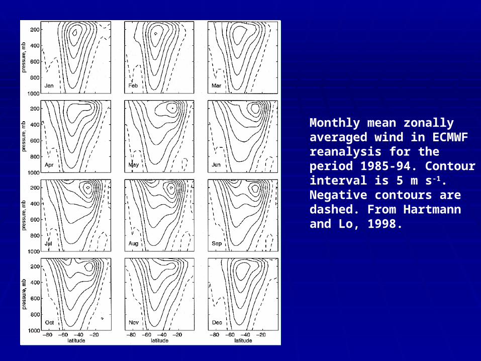
Parameterization

In the AMS-Glossary of Meteorology, parameterization is defined as “the representation in a dynamical model of physical effects in terms of admittedly oversimplified parameters, rather than realistically requiring such effects to be consequences of the dynamics of the system.”

Parameterization of Eddy FluxesParameterization of Eddy Fluxes









Why Potential Vorticity, Potential Temperature ?Why Potential Vorticity, Potential Temperature ?

350K

DqDt

=0q≡1σ 2Ωμ+ 1

a(1−μ2)∂V∂λ

⎛

⎝⎜⎜

⎞

⎠⎟⎟μ,θ

−1a∂U∂μ

⎛

⎝⎜⎜

⎞

⎠⎟⎟λ,θ

⎧

⎨⎪

⎩⎪

⎫

⎬⎪

⎭⎪

Ω

eλ

e

eλ

e

eθ

The Geometry of PVPT CoordinatesThe Geometry of PVPT Coordinates

λ

λ

λ

λ

e

yy

Transformation to PVPT CoordinatesTransformation to PVPT Coordinates

q

€

∂A∂λ

⎛ ⎝ ⎜

⎞ ⎠ ⎟μ ,θ

=∂A∂λ

⎛ ⎝ ⎜

⎞ ⎠ ⎟q,θ

−1h

∂A∂q

⎛

⎝ ⎜

⎞

⎠ ⎟λ ,θ

∂μ∂λ

⎛ ⎝ ⎜

⎞ ⎠ ⎟q,θ

€

∂A∂μ

⎛

⎝ ⎜

⎞

⎠ ⎟λ ,θ

=1h

∂A∂q

⎛

⎝ ⎜

⎞

⎠ ⎟λ ,θ

€

h =∂μ∂q

⎛

⎝ ⎜

⎞

⎠ ⎟λ ,θ

PV-thickness(Kushner and Held 1999)

€

μ =sinϕ

The Continuity EquationThe Continuity Equation

∂σ∂t

⎛

⎝⎜⎜

⎞

⎠⎟⎟μ ,θ

+ 1a

∂∂λ

σ U

1−μ 2

⎛

⎝

⎜⎜

⎞

⎠

⎟⎟

⎧

⎨⎪

⎩⎪

⎫

⎬⎪

⎭⎪μ ,θ

+ 1a

∂∂μ

σ V( )

⎧⎨⎪

⎩⎪

⎫⎬⎪

⎭⎪λ ,θ+ ∂

∂θσ &θ⎛

⎝⎜⎞

⎠⎟

⎧⎨⎪

⎩⎪

⎫⎬⎪

⎭⎪λ ,μ= 0

∂∂t

σ h( )

⎧⎨⎪

⎩⎪

⎫⎬⎪

⎭⎪q,θ+ 1

a∂

∂λσ hU1− μ2

⎛

⎝

⎜⎜⎜

⎞

⎠

⎟⎟⎟

⎧

⎨⎪

⎩⎪

⎫

⎬⎪

⎭⎪q,θ

+ ∂∂q

σ h &q( )

⎧⎨⎪

⎩⎪

⎫⎬⎪

⎭⎪λ ,θ+ ∂

∂θσ h &θ⎛

⎝⎜⎞

⎠⎟

⎧⎨⎪

⎩⎪

⎫⎬⎪

⎭⎪λ ,q= 0

Isentropic coordinates

PVPT coordinates

ρθ ≡σ

ρq ≡σ h

θ

q

λ€

ρqU −∂ ρ qU( )

∂λδλ2

€

ρqU +∂ ρ qU( )

∂λδλ2

λ

θ

The flow through a PVPT tubeThe flow through a PVPT tube

∂∂t

σ h( )⎧⎨⎪

⎩⎪

⎫⎬⎪

⎭⎪q,θ+ 1

a∂∂λ

σ hU1− μ2

⎛

⎝

⎜⎜

⎞

⎠

⎟⎟

⎧

⎨⎪

⎩⎪

⎫

⎬⎪

⎭⎪q,θ

+ ∂∂q

σ h &q( )⎧⎨⎪

⎩⎪

⎫⎬⎪

⎭⎪λ ,θ+ ∂

∂θσ h &θ⎛⎝⎜

⎞⎠⎟

⎧⎨⎪

⎩⎪

⎫⎬⎪

⎭⎪λ ,q= 0

0 0

Mass distribution on potential temperature and potential vorticity. Northern Hemisphere, January (a) and Northern Hemisphere, July (b) in NCEP-NCAR reanalysis

Mass Distribution in PVPT CoordinatesMass Distribution in PVPT Coordinates

a b

The Angular Momentum EquationThe Angular Momentum Equation

Isentropic coordinates PVPT coordinates

DLDt

+ ∂M∂λ

⎛

⎝⎜⎜

⎞

⎠⎟⎟μ,θ

=Xλ

DDt

= ∂∂t

⎛

⎝⎜⎞

⎠⎟λ,μ,θ+ U

a 1−μ2( )

∂∂λ

⎛

⎝⎜⎞

⎠⎟μ,θ+V

a∂∂μ

⎛

⎝⎜⎞

⎠⎟λ,θ+ &θ ∂

∂θ⎛

⎝⎜⎞

⎠⎟λ,μ

DLDt

+ ∂M∂λ

⎛

⎝⎜⎜

⎞

⎠⎟⎟q,θ

−1h∂M∂q

⎛

⎝⎜⎜

⎞

⎠⎟⎟λ,θ

∂μ∂λ

⎛

⎝⎜⎜

⎞

⎠⎟⎟q,θ

⎧

⎨⎪

⎩⎪

⎫

⎬⎪

⎭⎪=Xλ

DDt

= ∂∂t

⎛

⎝⎜⎞

⎠⎟λ,q,θ+ U

a 1−μ2( )

∂∂λ

⎛

⎝⎜⎞

⎠⎟q,θ+ &q ∂

∂q⎛

⎝⎜⎞

⎠⎟λ,θ+ &θ ∂

∂θ⎛

⎝⎜⎞

⎠⎟λ,q

DDt

= ∂∂t

⎛

⎝⎜

⎞

⎠⎟λ,μ,θ

+ Ua 1−μ2⎛

⎝⎜⎞⎠⎟

∂∂λ

⎛

⎝⎜

⎞

⎠⎟μ,θ

+Va

∂∂μ

⎛

⎝⎜⎜

⎞

⎠⎟⎟λ,θ

Adiabatic, frictionless conditions

DDt

= ∂∂t

⎛

⎝⎜

⎞

⎠⎟λ,q,θ

+ Ua 1−μ2⎛

⎝⎜⎞⎠⎟

∂∂λ

⎛

⎝⎜

⎞

⎠⎟q,θ

Adiabatic, frictionless conditions

Constraints on the PVPT coordinatesConstraints on the PVPT coordinates

Potential temperature varies monotonically with height/pressure.

Potential vorticity varies monotonically with latitude.

QuickTime™ and aYUV420 codec decompressor

are needed to see this picture.

pcoordinates

∂θ∂t

⎛

⎝

⎜⎜

⎞

⎠

⎟⎟p

=− &θ

θcoordinates

∂σ∂t

⎛

⎝

⎜⎜

⎞

⎠

⎟⎟θ

=− ∂∂θ

σ &θ⎛

⎝⎜⎜

⎞

⎠⎟⎟

PVPTcoordinates

∂σh∂t

⎛

⎝

⎜⎜

⎞

⎠

⎟⎟q

=− ∂∂q

σ h &q⎛⎝⎜

⎞⎠⎟

No Dry Convective AdjustmentNo Dry Convective Adjustment





What happens?What happens?

in p-coordinates potential temperature is predicted by an ODE, which can be analytically integrated and gives

θ(t)=− &θΔt

in θcoordinates the pseudo-density σ is predicted by an advection equation, which is a PDE, and the pressure is diagnosed from the top to the bottom by adding the mass from the isentropic layers above.

p(θ+Δθ)=p(θ)+σΔθ

Dry Convective AdjustmentDry Convective Adjustment



time

∂q∂μ

⎛

⎝⎜⎜

⎞

⎠⎟⎟

− ∂θ∂p

⎛

⎝⎜⎜

⎞

⎠⎟⎟

convective/

baroclinic

instability

p/μ

0time

∂μ∂q

⎛

⎝⎜⎜

⎞

⎠⎟⎟− ∂p

∂θ⎛

⎝⎜⎜

⎞

⎠⎟⎟

θ

convective/

baroclinic

instability

0

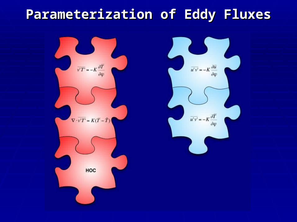
Hemispherical statistical distribution of regions where the PV gradient on θ=350K in ERA-40 reanalysis is negative for more than three consecutive days

January

350K NH

From Schubert et al., 1991

Momentum transport acting on Momentum transport acting on the zonal mean flowthe zonal mean flow

F=F(p)

∂∂t

σ hL⎡⎣⎢

⎤⎦⎥

⎧⎨⎪

⎩⎪

⎫⎬⎪

⎭⎪q,θ= 1

a∂∂θ

G ∂μ∂q

⎛

⎝⎜⎜

⎞

⎠⎟⎟λ ,θ

⎡

⎣

⎢⎢⎢

⎤

⎦

⎥⎥⎥

⎧

⎨⎪

⎩⎪

⎫

⎬⎪

⎭⎪λ ,q

− 1a

∂∂q

−F* ∂μ *∂λ

⎛

⎝⎜⎜

⎞

⎠⎟⎟q,θ

⎡

⎣

⎢⎢⎢

⎤

⎦

⎥⎥⎥+ G ∂μ

∂θ⎛

⎝⎜⎜

⎞

⎠⎟⎟λ ,q

⎡

⎣

⎢⎢⎢

⎤

⎦

⎥⎥⎥

⎧

⎨⎪

⎩⎪

⎫

⎬⎪

⎭⎪λ ,θ

G=pg

∂M∂λ

⎛

⎝⎜⎜

⎞

⎠⎟⎟μ,θ

−1a

∂∂q

−F* ∂μ *∂λ

⎛

⎝⎜⎜

⎞

⎠⎟⎟q,θ

⎡

⎣

⎢⎢⎢

⎤

⎦

⎥⎥⎥

⎧

⎨⎪

⎩⎪

⎫

⎬⎪

⎭⎪λ ,θ

1a

∂∂θ G ∂μ

∂q⎛

⎝⎜⎜

⎞

⎠⎟⎟λ,θ

⎡

⎣

⎢⎢

⎤

⎦

⎥⎥

⎧

⎨⎪

⎩⎪

⎫

⎬⎪

⎭⎪λ,q−1a

∂∂q

−F * ∂μ*∂λ

⎛

⎝⎜⎜

⎞

⎠⎟⎟q,θ

⎡

⎣

⎢⎢⎢

⎤

⎦

⎥⎥⎥

+ G ∂μ∂θ

⎛

⎝⎜⎜

⎞

⎠⎟⎟λ,q

⎡

⎣

⎢⎢⎢

⎤

⎦

⎥⎥⎥

⎧

⎨⎪

⎩⎪

⎫

⎬⎪

⎭⎪λ,θ

=0

Eliassen-Palm FluxEliassen-Palm Flux

∇⋅E = 0

E= 0,E q( ),E θ⎛⎝⎜

⎞⎠⎟

⎛

⎝⎜

⎞

⎠⎟

E q( ) = F * ∂μ*∂λ

⎛

⎝⎜⎜

⎞

⎠⎟⎟q,θ

⎡

⎣

⎢⎢⎢

⎤

⎦

⎥⎥⎥

− G ∂μ∂θ

⎛

⎝⎜⎜

⎞

⎠⎟⎟λ,q

⎡

⎣

⎢⎢⎢

⎤

⎦

⎥⎥⎥

Eθ⎛

⎝⎜⎞⎠⎟ = G ∂μ

∂q⎛

⎝⎜⎜

⎞

⎠⎟⎟λ,θ

⎡

⎣

⎢⎢

⎤

⎦

⎥⎥

E(ϕ )=−acosϕ[(σv)*u* ]

E(θ)=1g p* ∂M *

∂λ⎡

⎣⎢⎢

⎤

⎦⎥⎥

Isentropic Coordinates

Andrews et al., 1987

∂∂t

σ hL⎡⎣

⎤⎦

⎧⎨⎪

⎩⎪

⎫⎬⎪

⎭⎪q,θ= 1

a∂∂θ

G ∂μ∂q

⎛

⎝⎜⎜

⎞

⎠⎟⎟λ ,θ

⎡

⎣

⎢⎢

⎤

⎦

⎥⎥

⎧

⎨⎪

⎩⎪

⎫

⎬⎪

⎭⎪λ ,q

− 1a

∂∂q

−F* ∂μ *∂λ

⎛

⎝⎜⎜

⎞

⎠⎟⎟q,θ

⎡

⎣

⎢⎢⎢

⎤

⎦

⎥⎥⎥

+ G ∂μ∂θ

⎛

⎝⎜⎜

⎞

⎠⎟⎟λ ,q

⎡

⎣

⎢⎢⎢

⎤

⎦

⎥⎥⎥

⎧

⎨⎪

⎩⎪

⎫

⎬⎪

⎭⎪λ ,θ

Residual Circulation in PVPTResidual Circulation in PVPT

€

˙ ˆ q =∇ ⋅Jq

[σ ]

€

˙ ˆ θ = Q

Data used in these plots are simulated with Ross Heikes isentropic model

ConclusionsConclusions

1.) Introduction of potential vorticity as meridional coordinate.

The merdional advection is zero for an adiabatic, frictionless flow.

In connection with the potential temperature the newly created system of

coordinates allows to divide the atmosphere into undulating tubes bounded by

isentropic and constant PV surfaces, and the air moves through these tubes

without penetrating through the walls.

A numerical model that uses the PVPT system has the advantage of incorporating

as “built-in” dry convective and baroclinic adjustment processes.

ConclusionsConclusions

2.) Develop a framework adequate for parameterization of the eddy

momentum transport.

When applied to the study of the mean meridional circulation the PVPT system of

coordinates reveals a residual circulation driven by the Lagrangian time rate of

change of the PV and θ

The momentum exchange that affects the zonal mean flow - zonal component of

the pressure forces exerted by the eddies on a thin zonal tube bounded by surfaces

of constant PV as lateral sides and undulating bottom and top isentropes.

PerspectivesPerspectives

What could be the applications of the PVPT system of coordinates in climate studies?

PVPT framework emerges at the same time with the ERA 40 reanalysisproducts, which provide direct model outputs on the PV surface 2PVU.

As model resolution changes the need for parameterization does not simply go away. Simple zonally averaged models provide test beds for understanding hypothesized mechanisms.

Documents

The Mean Meridional Circulation: A New Potential-Vorticity, Potential- Temperature Perspective Cristiana Stan Colorado State University March 11, 2005