1

BBAA VI International Colloquium on: Bluff Bodies Aerodynamics & Applications

Milano, Italy, July, 20-24 2008

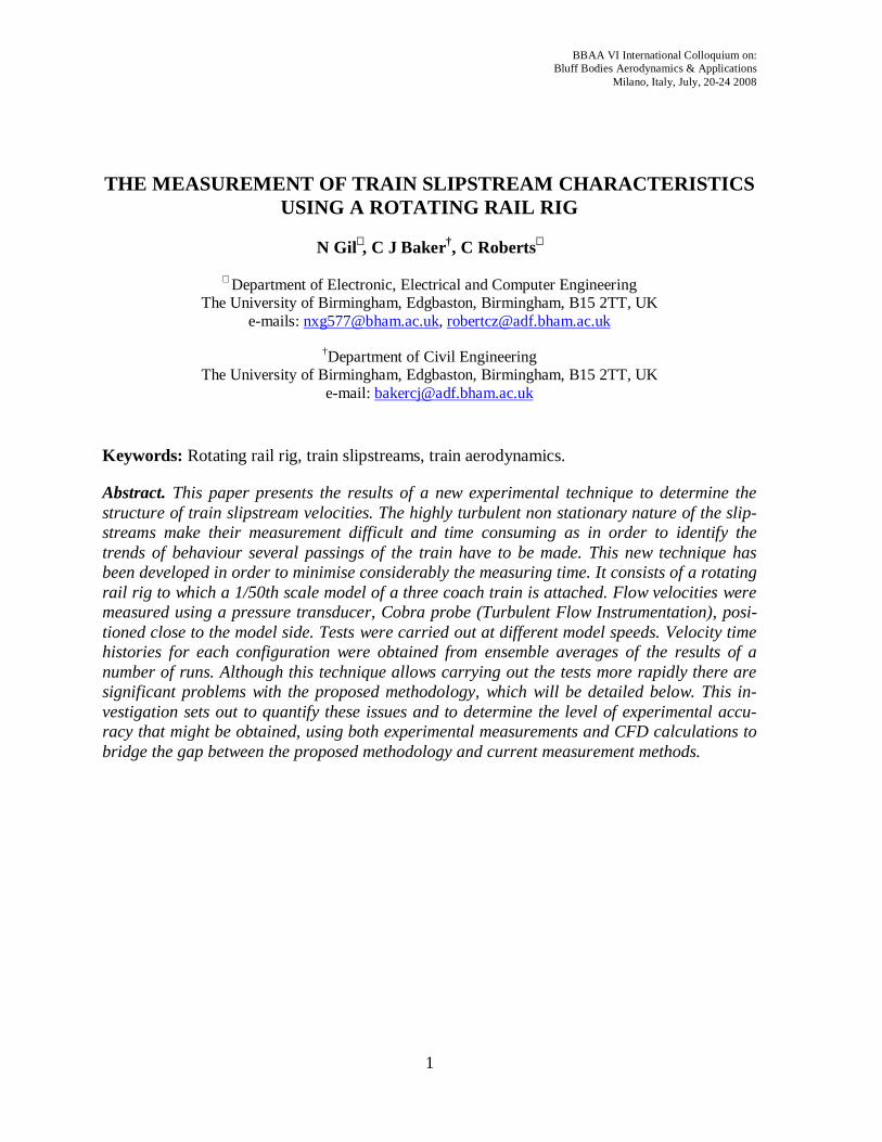
THE MEASUREMENT OF TRAIN SLIPSTREAM CHARACTERISTICS USING A ROTATING RAIL RIG

N Gil∗ , C J Baker†, C Roberts∗

∗ Department of Electronic, Electrical and Computer Engineering The University of Birmingham, Edgbaston, Birmingham, B15 2TT, UK

e-mails: nxg577@bham.ac.uk, robertcz@adf.bham.ac.uk

†Department of Civil Engineering The University of Birmingham, Edgbaston, Birmingham, B15 2TT, UK

e-mail: bakercj@adf.bham.ac.uk

Keywords: Rotating rail rig, train slipstreams, train aerodynamics.

Abstract. This paper presents the results of a new experimental technique to determine the structure of train slipstream velocities. The highly turbulent non stationary nature of the slip-streams make their measurement difficult and time consuming as in order to identify the trends of behaviour several passings of the train have to be made. This new technique has been developed in order to minimise considerably the measuring time. It consists of a rotating rail rig to which a 1/50th scale model of a three coach train is attached. Flow velocities were measured using a pressure transducer, Cobra probe (Turbulent Flow Instrumentation), posi-tioned close to the model side. Tests were carried out at different model speeds. Velocity time histories for each configuration were obtained from ensemble averages of the results of a number of runs. Although this technique allows carrying out the tests more rapidly there are significant problems with the proposed methodology, which will be detailed below. This in-vestigation sets out to quantify these issues and to determine the level of experimental accu-racy that might be obtained, using both experimental measurements and CFD calculations to bridge the gap between the proposed methodology and current measurement methods.

N. Gil, C. J. Baker and C. Roberts

2

1 INTRODUCTION

The movement of high speed trains through the atmosphere can result in significant air flow velocities at the side and in the wake of such vehicles. These velocities can in turn pose a safety risk for passengers and trackside workers, and can cause problems for pushchairs and luggage trolleys. These safety concerns have led to significant work in this field over recent years and a number of full scale and model scale tests have been carried out to measure these slipstream velocities. As shown in section 2, the data obtained for each train type, operating speed and wind condition is usually sparse due to the random behaviour of the flow. Further-more, the European Standards state [1] that to identify the trends of behaviour at least 20 comparable samples (in terms of train type, speed and wind condition) are required at each measurement point. This would imply the spending of a significant amount of money and time on an issue that is not even seen as a major hazard within the overall railway risk in the UK[1]. Therefore, there is a need to obtain this information more rapidly and at a considera-bly lower cost and this is precisely what this project is dealing with.

This paper presents the results of a different type of technique that uses an experimental set up known as a rotating rail rig that in principle allows such tests to be carried out much more rapidly. It consists of a 3.61 diameter rotating rail rig to which a 1/50th scale model of a three coach train is attached. Flow velocities are measured using a pressure transducer, Cobra probe (Turbulent Flow Instrumentation), at different positions from the model side. Tests have been carried out at different model speeds of 4.725, 9.45 and 14.175 m/s)

The experimental configurations and conditions are described in section 3. This section also includes an explanation of the problems with this technique as, although the results are promising, there are significant issues with the proposed methodology that have to be taken into account. The slipstream velocities results at different train speed and distances of the probe from the train side are shown and discussed in section 4. Finally, section 5 presents the conclusions and recommendations for further work.

2 CURRENT METHODS FOR MEASURING TRAIN SLIPSTREAM VELOCITIES

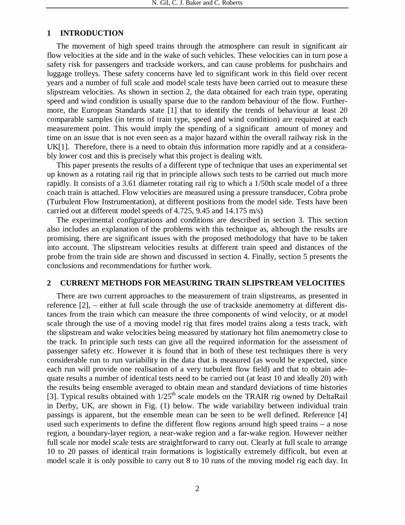
There are two current approaches to the measurement of train slipstreams, as presented in reference [2], – either at full scale through the use of trackside anemometry at different dis-tances from the train which can measure the three components of wind velocity, or at model scale through the use of a moving model rig that fires model trains along a tests track, with the slipstream and wake velocities being measured by stationary hot film anemometry close to the track. In principle such tests can give all the required information for the assessment of passenger safety etc. However it is found that in both of these test techniques there is very considerable run to run variability in the data that is measured (as would be expected, since each run will provide one realisation of a very turbulent flow field) and that to obtain ade-quate results a number of identical tests need to be carried out (at least 10 and ideally 20) with the results being ensemble averaged to obtain mean and standard deviations of time histories [3]. Typical results obtained with 1/25th scale models on the TRAIR rig owned by DeltaRail in Derby, UK, are shown in Fig. (1) below. The wide variability between individual train passings is apparent, but the ensemble mean can be seen to be well defined. Reference [4] used such experiments to define the different flow regions around high speed trains – a nose region, a boundary-layer region, a near-wake region and a far-wake region. However neither full scale nor model scale tests are straightforward to carry out. Clearly at full scale to arrange 10 to 20 passes of identical train formations is logistically extremely difficult, but even at model scale it is only possible to carry out 8 to 10 runs of the moving model rig each day. In

N. Gil, C. J. Baker and C. Roberts

3

Normalised velocities from individual runs and from ensemble average

0

0.5

1

-5 0 5 10 15 20 25

t

Run A

Run B

Run C

Run D

Run E

25 run ensemble

both cases obtaining the same train or model velocity over a number of runs, so that the en-semble average can be calculated is also far from straightforward.

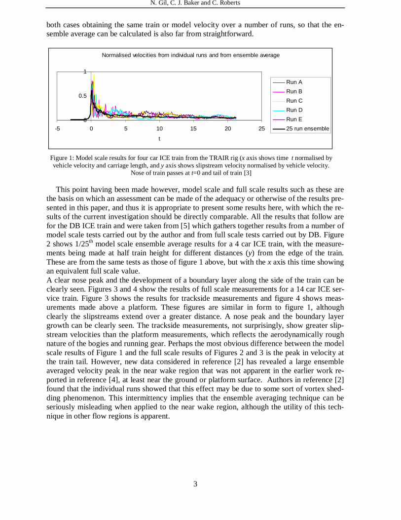
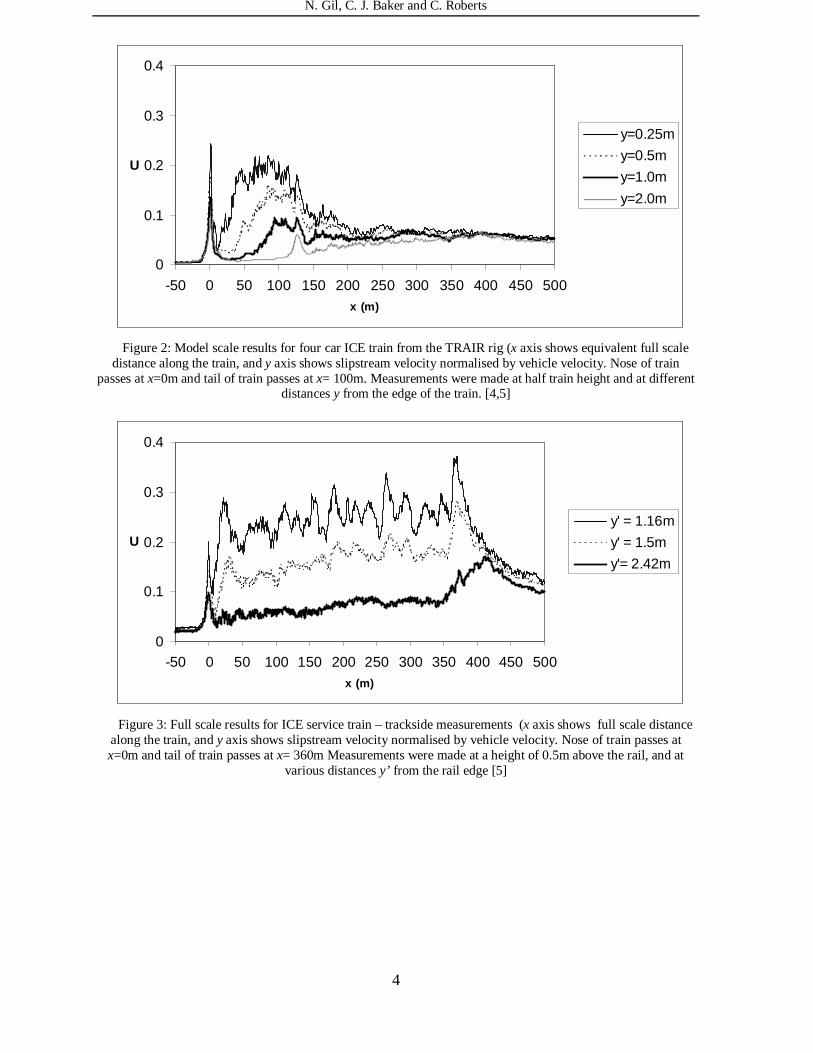
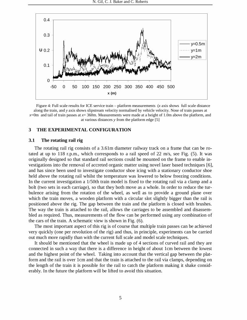
This point having been made however, model scale and full scale results such as these are the basis on which an assessment can be made of the adequacy or otherwise of the results pre-sented in this paper, and thus it is appropriate to present some results here, with which the re-sults of the current investigation should be directly comparable. All the results that follow are for the DB ICE train and were taken from [5] which gathers together results from a number of model scale tests carried out by the author and from full scale tests carried out by DB. Figure 2 shows 1/25th model scale ensemble average results for a 4 car ICE train, with the measure-ments being made at half train height for different distances (y) from the edge of the train. These are from the same tests as those of figure 1 above, but with the x axis this time showing an equivalent full scale value. A clear nose peak and the development of a boundary layer along the side of the train can be clearly seen. Figures 3 and 4 show the results of full scale measurements for a 14 car ICE ser-vice train. Figure 3 shows the results for trackside measurements and figure 4 shows meas-urements made above a platform. These figures are similar in form to figure 1, although clearly the slipstreams extend over a greater distance. A nose peak and the boundary layer growth can be clearly seen. The trackside measurements, not surprisingly, show greater slip-stream velocities than the platform measurements, which reflects the aerodynamically rough nature of the bogies and running gear. Perhaps the most obvious difference between the model scale results of Figure 1 and the full scale results of Figures 2 and 3 is the peak in velocity at the train tail. However, new data considered in reference [2] has revealed a large ensemble averaged velocity peak in the near wake region that was not apparent in the earlier work re-ported in reference [4], at least near the ground or platform surface. Authors in reference [2] found that the individual runs showed that this effect may be due to some sort of vortex shed-ding phenomenon. This intermittency implies that the ensemble averaging technique can be seriously misleading when applied to the near wake region, although the utility of this tech-nique in other flow regions is apparent.

Figure 1: Model scale results for four car ICE train from the TRAIR rig (x axis shows time t normalised by vehicle velocity and carriage length, and y axis shows slipstream velocity normalised by vehicle velocity.

Nose of train passes at t=0 and tail of train [3]

N. Gil, C. J. Baker and C. Roberts

4

0

0.1

0.2

0.3

0.4

-50 0 50 100 150 200 250 300 350 400 450 500x (m)

U

y=0.25m

y=0.5m

y=1.0m

y=2.0m

Figure 2: Model scale results for four car ICE train from the TRAIR rig (x axis shows equivalent full scale

distance along the train, and y axis shows slipstream velocity normalised by vehicle velocity. Nose of train passes at x=0m and tail of train passes at x= 100m. Measurements were made at half train height and at different

distances y from the edge of the train. [4,5]

0

0.1

0.2

0.3

0.4

-50 0 50 100 150 200 250 300 350 400 450 500x (m)

U

y' = 1.16m

y' = 1.5m

y'= 2.42m

Figure 3: Full scale results for ICE service train – trackside measurements (x axis shows full scale distance

along the train, and y axis shows slipstream velocity normalised by vehicle velocity. Nose of train passes at x=0m and tail of train passes at x= 360m Measurements were made at a height of 0.5m above the rail, and at

various distances y’ from the rail edge [5]

N. Gil, C. J. Baker and C. Roberts

5

0

0.1

0.2

0.3

0.4

-50 0 50 100 150 200 250 300 350 400 450 500x (m)

U

y=0.5m

y=1m

y=2m

Figure 4: Full scale results for ICE service train – platform measurements (x axis shows full scale distance

along the train, and y axis shows slipstream velocity normalised by vehicle velocity. Nose of train passes at x=0m and tail of train passes at x= 360m. Measurements were made at a height of 1.0m above the platform, and

at various distances y from the platform edge [5]

3 THE EXPERIMENTAL CONFIGURATION

3.1 The rotating rail rig

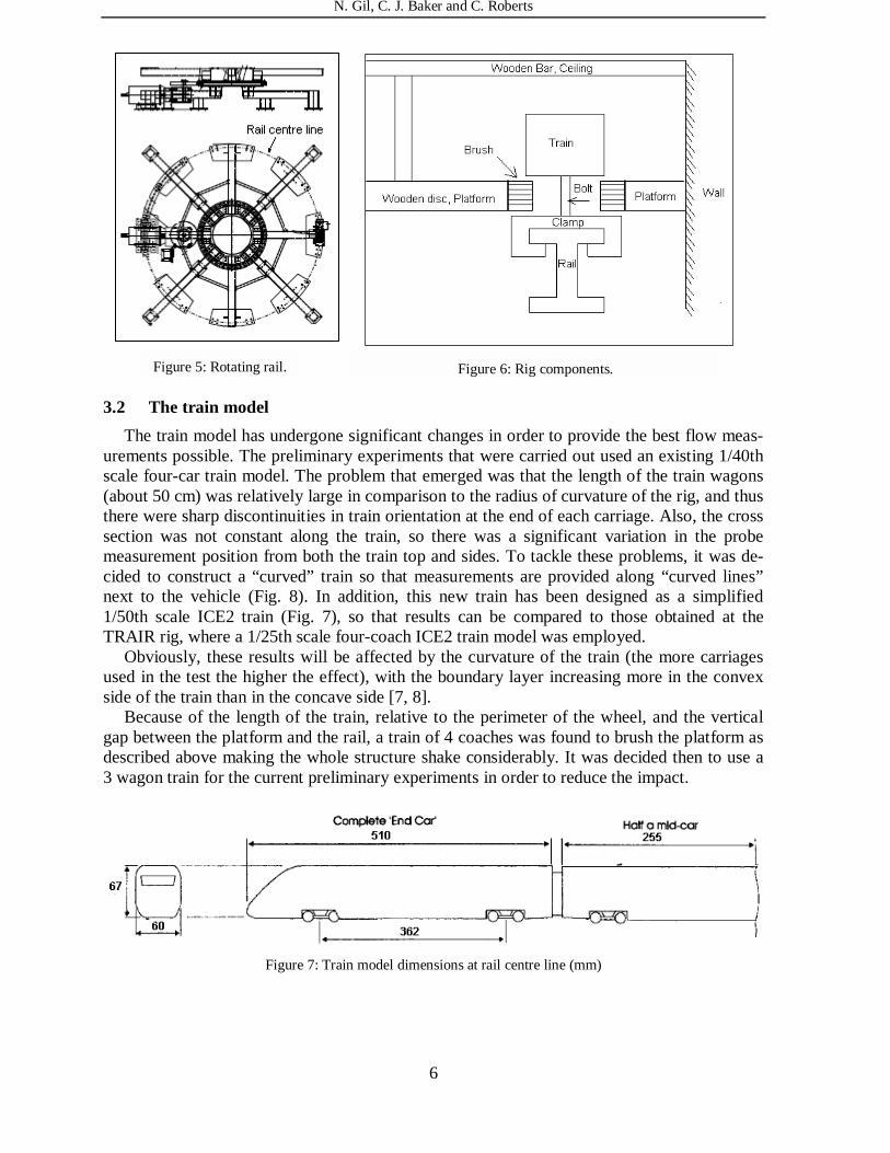
The rotating rail rig consists of a 3.61m diameter railway track on a frame that can be ro-tated at up to 118 r.p.m., which corresponds to a rail speed of 22 m/s, see Fig. (5). It was originally designed so that standard rail sections could be mounted on the frame to enable in-vestigations into the removal of accreted organic matter using novel laser based techniques [6], and has since been used to investigate conductor shoe icing with a stationary conductor shoe held above the rotating rail whilst the temperature was lowered to below freezing conditions. In the current investigation a 1/50th train model is fixed to the rotating rail via a clamp and a bolt (two sets in each carriage), so that they both move as a whole. In order to reduce the tur-bulence arising from the rotation of the wheel, as well as to provide a ground plane over which the train moves, a wooden platform with a circular slot slightly bigger than the rail is positioned above the rig. The gap between the train and the platform is closed with brushes. The way the train is attached to the rail, allows the carriages to be assembled and disassem-bled as required. Thus, measurements of the flow can be performed using any combination of the cars of the train. A schematic view is shown in Fig. (6).

The most important aspect of this rig is of course that multiple train passes can be achieved very quickly (one per revolution of the rig) and thus, in principle, experiments can be carried out much more rapidly than with the current full scale and model scale techniques.

It should be mentioned that the wheel is made up of 4 sections of curved rail and they are connected in such a way that there is a difference in height of about 1cm between the lowest and the highest point of the wheel. Taking into account that the vertical gap between the plat-form and the rail is over 1cm and that the train is attached to the rail via clamps, depending on the length of the train it is possible for the rail to catch the platform making it shake consid-erably. In the future the platform will be lifted to avoid this situation.

N. Gil, C. J. Baker and C. Roberts

6

3.2 The train model

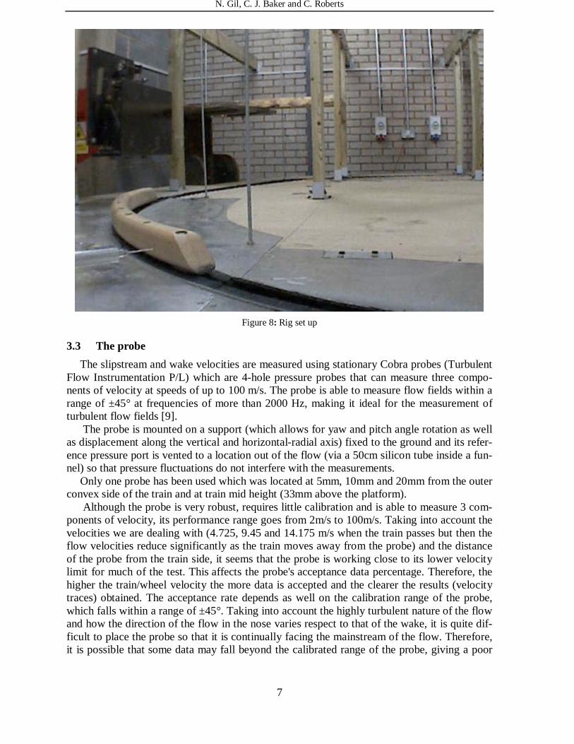
The train model has undergone significant changes in order to provide the best flow meas-urements possible. The preliminary experiments that were carried out used an existing 1/40th scale four-car train model. The problem that emerged was that the length of the train wagons (about 50 cm) was relatively large in comparison to the radius of curvature of the rig, and thus there were sharp discontinuities in train orientation at the end of each carriage. Also, the cross section was not constant along the train, so there was a significant variation in the probe measurement position from both the train top and sides. To tackle these problems, it was de-cided to construct a “curved” train so that measurements are provided along “curved lines” next to the vehicle (Fig. 8). In addition, this new train has been designed as a simplified 1/50th scale ICE2 train (Fig. 7), so that results can be compared to those obtained at the TRAIR rig, where a 1/25th scale four-coach ICE2 train model was employed.

Obviously, these results will be affected by the curvature of the train (the more carriages used in the test the higher the effect), with the boundary layer increasing more in the convex side of the train than in the concave side [7, 8].

Because of the length of the train, relative to the perimeter of the wheel, and the vertical gap between the platform and the rail, a train of 4 coaches was found to brush the platform as described above making the whole structure shake considerably. It was decided then to use a 3 wagon train for the current preliminary experiments in order to reduce the impact.

Figure 7: Train model dimensions at rail centre line (mm)

Figure 5: Rotating rail. Figure 6: Rig components.

N. Gil, C. J. Baker and C. Roberts

7

Figure 8: Rig set up

3.3 The probe

The slipstream and wake velocities are measured using stationary Cobra probes (Turbulent Flow Instrumentation P/L) which are 4-hole pressure probes that can measure three compo-nents of velocity at speeds of up to 100 m/s. The probe is able to measure flow fields within a range of ±45° at frequencies of more than 2000 Hz, making it ideal for the measurement of turbulent flow fields [9].

The probe is mounted on a support (which allows for yaw and pitch angle rotation as well as displacement along the vertical and horizontal-radial axis) fixed to the ground and its refer-ence pressure port is vented to a location out of the flow (via a 50cm silicon tube inside a fun-nel) so that pressure fluctuations do not interfere with the measurements.

Only one probe has been used which was located at 5mm, 10mm and 20mm from the outer convex side of the train and at train mid height (33mm above the platform).

Although the probe is very robust, requires little calibration and is able to measure 3 com-ponents of velocity, its performance range goes from 2m/s to 100m/s. Taking into account the velocities we are dealing with (4.725, 9.45 and 14.175 m/s when the train passes but then the flow velocities reduce significantly as the train moves away from the probe) and the distance of the probe from the train side, it seems that the probe is working close to its lower velocity limit for much of the test. This affects the probe's acceptance data percentage. Therefore, the higher the train/wheel velocity the more data is accepted and the clearer the results (velocity traces) obtained. The acceptance rate depends as well on the calibration range of the probe, which falls within a range of ±45°. Taking into account the highly turbulent nature of the flow and how the direction of the flow in the nose varies respect to that of the wake, it is quite dif-ficult to place the probe so that it is continually facing the mainstream of the flow. Therefore, it is possible that some data may fall beyond the calibrated range of the probe, giving a poor

N. Gil, C. J. Baker and C. Roberts

8

acceptance rate. The probe working voltage is 5V, so very low signals are being measured especially when the train is not passing in front of the probe. In addition, electrical noise and vibrations are also present. In order to reduce the noise, Matlab filtering at 312.5HZ has been carried out.

3.4 Tests

Different tests have been carried out. In order to study the slipstream velocity results de-pendence with train speed, it was decided to run the wheel at velocities of 4.725, 9.45 and 14.175 m/s, with the probe located at train mid height (33mm above the platform). Velocities above 14.175 m/s endanger the stability of the structure mounted around the wheel, so until changes are made this is the maximum velocity that can be achieved. In order to let the air flow stabilise in the room, the train was allowed to go round for a reasonable time before tak-ing any measurements. As shown later on, there seems to be a low velocity ongoing airflow around the wheel.

In order to get measurements every 1-2 mm of the train, depending on the train speed, sampling frequencies of 3000Hz were adequate so by the Nyquist rule, the final sampling fre-quency was set to 6000Hz.

As mentioned before 3 carriages of the 1/50th model scale train were used (each carriage of 510mm, which corresponds to a equivalent full scale length of 25m) and the probe located always at train mid height and always taking measurements from the outer surface of the train, taking y=0 the surface of the train ( y is the perpendicular distance, in meters, to the tangent of the train surface).

In order to check for vibrations and electrical noise, the reference port and the head of the probe (where the pressure taps are found) were connected using a tube, and voltages values on the four different channels were assessed for three different cases: a) No movement of the wheel, b) the wheel spinning at different velocities and, c) freewheeling. The results obtained will be discussed in the following section.

As a summary, the following tables show the different tests carried out.

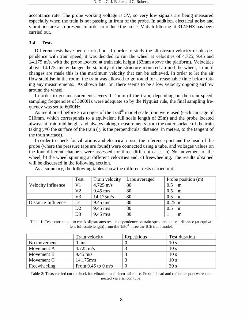
Test Train velocity Laps averaged Probe position (m) Velocity Influence V1 4.725 m/s 80 0.5 m V2 9.45 m/s 80 0.5 m V3 14.175m/s 80 0.5 m Distance Influence D1 9.45 m/s 80 0.25 m D2 9.45 m/s 80 0.5 m D3 9.45 m/s 80 1 m

Table 1: Tests carried out to check slipstreams results dependence on train speed and lateral distance (at equiva-lent full scale length) from the 1/50th three car ICE train model.

Train velocity Repetitions Test duration No movement 0 m/s 0 10 s Movement A 4.725 m/s 3 10 s Movement B 9.45 m/s 3 10 s Movement C 14.175m/s 3 10 s Freewheeling From 9.45 to 0 m/s 0 30 s

Table 2: Tests carried out to check for vibration and electrical noise. Probe’s head and reference port were con-nected via a silicon tube.

N. Gil, C. J. Baker and C. Roberts

9

4 EXPERIMENTAL RESULTS

As in previous studies [2,5] the coordinate system used is such that the x-axis follows the train direction of travel (as an individual sees it from the platform edge) , with the origin taken to be when the nose of the train passes the measuring point , and the y-axis is in the horizontal plane perpendicular to the track. Taking into account the rig presented here is circular, then the x and y axis are tangent and perpendicular to the rail respectively.

As mentioned before the probe is situated at train mid height in every test, which corre-sponds to a distance of 33 mm above the platform.

For comparison purposes, as different train velocities have been tested, the ensemble mean velocity and standard deviations results have been normalised by train speed.

Section 2 stated that to obtain adequate results a number of identical tests need to be car-ried out (at least 10 and ideally 20) with the results being ensemble averaged to obtain mean and standard deviations of time histories [3]. Taking advantage of the capability of the rig, in this paper, 80 laps have been averaged.

4.1 Preliminary considerations

Originally the probe was mounted on a support fixed to one of the four legs that sustain the wheel (bottom left leg in Figure 2). Tests at different velocities were carried out and the re-sults obtained were not very clear as the nose peak was not visible. A position sensor that gave an impulse signal when the train passed, was used in order to identify the train slip-streams within the signal, and only after ensemble averaging all the laps was it possible to identify the “train”. Three main problems were found to be causing this lack of clarity in the data results: the probe calibration problems mentioned above (section 3.2), electrical noise, and significant vibrations transmitted through the mounting system.

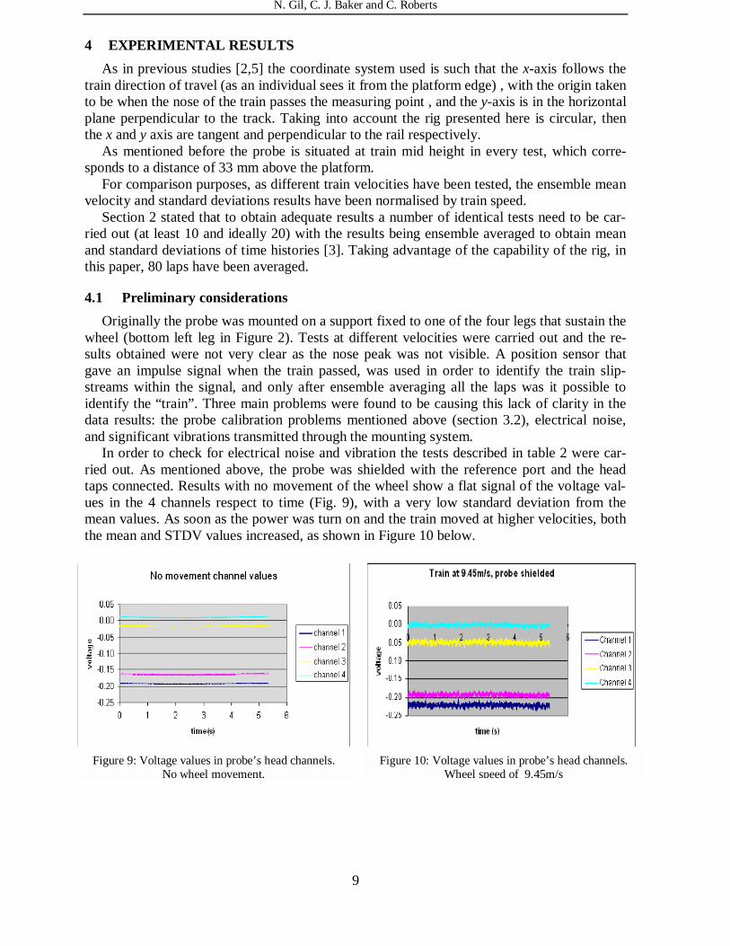
In order to check for electrical noise and vibration the tests described in table 2 were car-ried out. As mentioned above, the probe was shielded with the reference port and the head taps connected. Results with no movement of the wheel show a flat signal of the voltage val-ues in the 4 channels respect to time (Fig. 9), with a very low standard deviation from the mean values. As soon as the power was turn on and the train moved at higher velocities, both the mean and STDV values increased, as shown in Figure 10 below.

Figure 9: Voltage values in probe’s head channels. No wheel movement.

Figure 10: Voltage values in probe’s head channels. Wheel speed of 9.45m/s

N. Gil, C. J. Baker and C. Roberts

10

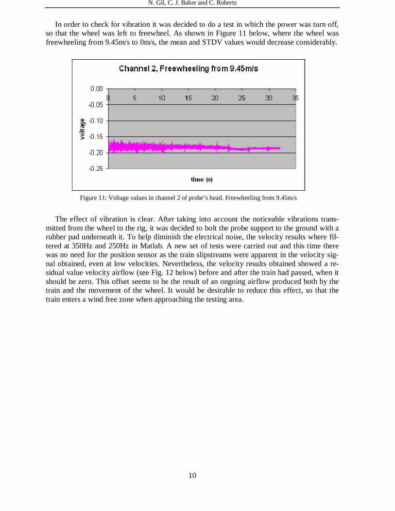
In order to check for vibration it was decided to do a test in which the power was turn off, so that the wheel was left to freewheel. As shown in Figure 11 below, where the wheel was freewheeling from 9.45m/s to 0m/s, the mean and STDV values would decrease considerably.

The effect of vibration is clear. After taking into account the noticeable vibrations trans-

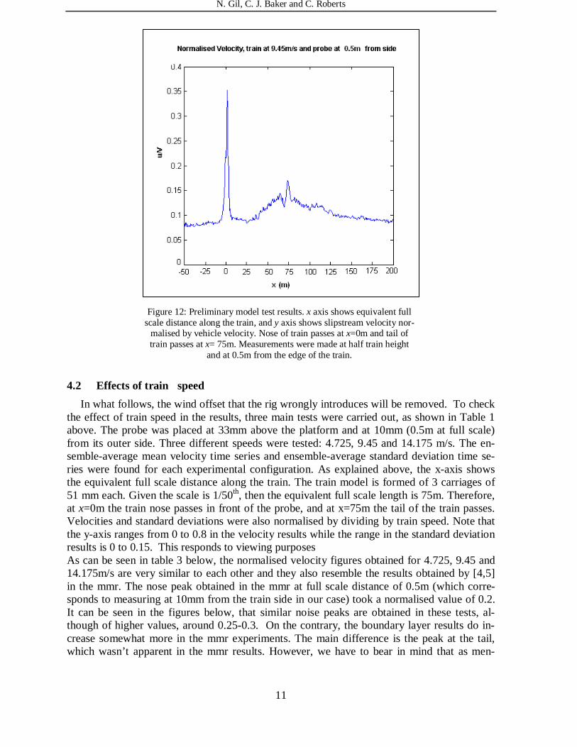
mitted from the wheel to the rig, it was decided to bolt the probe support to the ground with a rubber pad underneath it. To help diminish the electrical noise, the velocity results where fil-tered at 350Hz and 250Hz in Matlab. A new set of tests were carried out and this time there was no need for the position sensor as the train slipstreams were apparent in the velocity sig-nal obtained, even at low velocities. Nevertheless, the velocity results obtained showed a re-sidual value velocity airflow (see Fig. 12 below) before and after the train had passed, when it should be zero. This offset seems to be the result of an ongoing airflow produced both by the train and the movement of the wheel. It would be desirable to reduce this effect, so that the train enters a wind free zone when approaching the testing area.

Figure 11: Voltage values in channel 2 of probe’s head. Freewheeling from 9.45m/s

N. Gil, C. J. Baker and C. Roberts

11

4.2 Effects of train speed

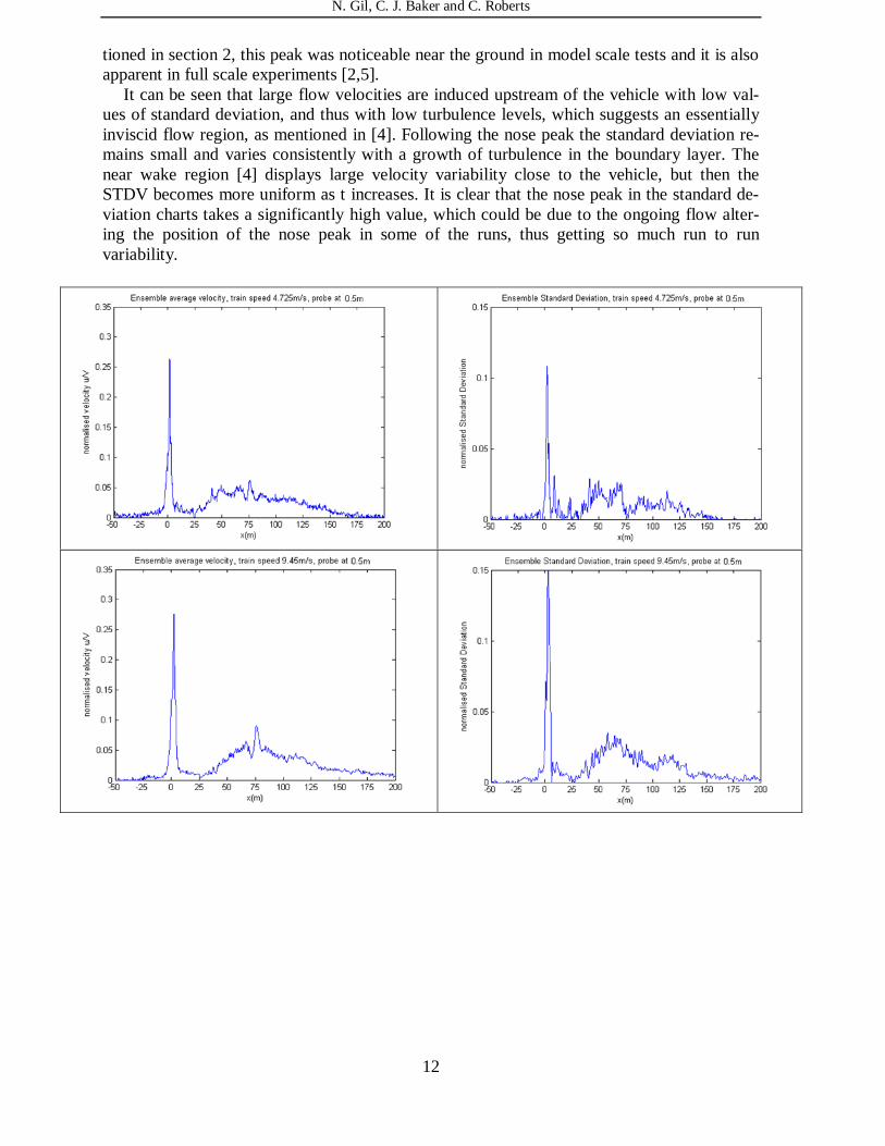
In what follows, the wind offset that the rig wrongly introduces will be removed. To check the effect of train speed in the results, three main tests were carried out, as shown in Table 1 above. The probe was placed at 33mm above the platform and at 10mm (0.5m at full scale) from its outer side. Three different speeds were tested: 4.725, 9.45 and 14.175 m/s. The en-semble-average mean velocity time series and ensemble-average standard deviation time se-ries were found for each experimental configuration. As explained above, the x-axis shows the equivalent full scale distance along the train. The train model is formed of 3 carriages of 51 mm each. Given the scale is 1/50th, then the equivalent full scale length is 75m. Therefore, at x=0m the train nose passes in front of the probe, and at x=75m the tail of the train passes. Velocities and standard deviations were also normalised by dividing by train speed. Note that the y-axis ranges from 0 to 0.8 in the velocity results while the range in the standard deviation results is 0 to 0.15. This responds to viewing purposes As can be seen in table 3 below, the normalised velocity figures obtained for 4.725, 9.45 and 14.175m/s are very similar to each other and they also resemble the results obtained by [4,5] in the mmr. The nose peak obtained in the mmr at full scale distance of 0.5m (which corre-sponds to measuring at 10mm from the train side in our case) took a normalised value of 0.2. It can be seen in the figures below, that similar noise peaks are obtained in these tests, al-though of higher values, around 0.25-0.3. On the contrary, the boundary layer results do in-crease somewhat more in the mmr experiments. The main difference is the peak at the tail, which wasn’t apparent in the mmr results. However, we have to bear in mind that as men-

Figure 12: Preliminary model test results. x axis shows equivalent full scale distance along the train, and y axis shows slipstream velocity nor-

malised by vehicle velocity. Nose of train passes at x=0m and tail of train passes at x= 75m. Measurements were made at half train height

and at 0.5m from the edge of the train.

N. Gil, C. J. Baker and C. Roberts

12

tioned in section 2, this peak was noticeable near the ground in model scale tests and it is also apparent in full scale experiments [2,5].

It can be seen that large flow velocities are induced upstream of the vehicle with low val-ues of standard deviation, and thus with low turbulence levels, which suggests an essentially inviscid flow region, as mentioned in [4]. Following the nose peak the standard deviation re-mains small and varies consistently with a growth of turbulence in the boundary layer. The near wake region [4] displays large velocity variability close to the vehicle, but then the STDV becomes more uniform as t increases. It is clear that the nose peak in the standard de-viation charts takes a significantly high value, which could be due to the ongoing flow alter-ing the position of the nose peak in some of the runs, thus getting so much run to run variability.

N. Gil, C. J. Baker and C. Roberts

13

Table 3: Ensemble average velocities and standard deviations for train speeds of 4.725m/s, 9.45m/s and 14.175m/s. Probe located in all three cases at full scale distance of 0.5m from the model side.

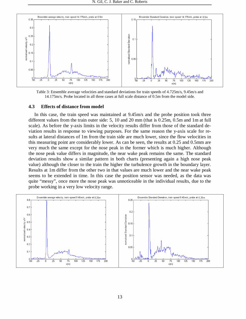
4.3 Effects of distance from model

In this case, the train speed was maintained at 9.45m/s and the probe position took three different values from the train outer side: 5, 10 and 20 mm (that is 0.25m, 0.5m and 1m at full scale). As before the y-axis limits in the velocity results differ from those of the standard de-viation results in response to viewing purposes. For the same reason the y-axis scale for re-sults at lateral distances of 1m from the train side are much lower, since the flow velocities in this measuring point are considerably lower. As can be seen, the results at 0.25 and 0.5mm are very much the same except for the nose peak in the former which is much higher. Although the nose peak value differs in magnitude, the near wake peak remains the same. The standard deviation results show a similar pattern in both charts (presenting again a high nose peak value) although the closer to the train the higher the turbulence growth in the boundary layer. Results at 1m differ from the other two in that values are much lower and the near wake peak seems to be extended in time. In this case the position sensor was needed, as the data was quite “messy”, once more the nose peak was unnoticeable in the individual results, due to the probe working in a very low velocity range.

N. Gil, C. J. Baker and C. Roberts

14

Table 4: Ensemble average velocities and standard deviations for measuring points at half train height and at

distances of 0.25m, 0.5m and 1m from the model side. Train speed maintained at 9.45m/s.

5 CONCLUDING REMARKS

The results shown in section 4 are very encouraging as not only the four main flow regions (nose , boundary layer, near wake and far wake) mentioned in section 2 can be identified in the charts but results also resemble the experimental results obtained in the Moving Model Rig [4], where a 1/25th scale ICE2 train was used. Furthermore, the rig provided 80 laps at quite a short period of time (1min for wheel speeds of 14.175m/s), showing again the great advantage of the rig against conventional methods.

There is however the issue of an actual wind offset of around 0.1 of the wheel velocity that seems to be the result of an ongoing airflow produced both by the train and the movement of the wheel. Various alternatives will be considered in order to reduce this offset.

Further experiments with the probe situated in the inner side of the train will be carried out. Measuring points will be defined at different distances from the train side and top and at dif-ferent heights, so that results in the top of the train and its concave and the convex sides can be compared and discussed. In order to analyse the turbulence and flow structures wavelet analysis of the individual runs will be carried out.

To understand further the effects on the results introduced by the curvature of the rig, a se-ries of CFD calculations will be carried out which will be validated using the experimental results obtained in the rig. A very simple first simulation was carried out in ANSYS where the model was defined using a quarter of the track. An inner section containing the track and the

N. Gil, C. J. Baker and C. Roberts

15

train moved at 10rpm (1.57 m/s) through an outer section defined by the platform and still air surrounding the train. A moving frame of reference, a sliding coarse mesh and periodic boundaries at each end of the section were defined to reproduce the motion of the passing train. The k-epsilon turbulence model was employed and the simulation defined as steady state. The probe was located at half height of the train at 1cm from the outer side of the vehi-cle. The results resemble as well those of [4, 5]. They also show the near wake peak present in the spinning-rail experimental results. Furthermore, the wind offset is also present in the CFD results. Further CFD calculations will also be carried out for larger track and model radii, and will include the modelling of the straight track. The results for the different curvatures will then be compared, which should enable a judgement to be made concerning the minimum ra-dius of such a rig that will enable the slipstream results obtained to be representative of the full scale situation and thus to make recommendations for the design of a larger more repre-sentative rig that retains the utility of being able to simulate many train passes rapidly whilst being more representative of reality.

ACKNOWLEDGEMENTS

The authors wish to acknowledge the help of Dr David Hargreaves for providing the CFD model and calculations, Mr. Andy Dunn for his technical support, Dr. Paul Weston and Dr. Edward Stewart for providing the position sensor and EECE for granting the studentship.

REFERENCES

[1] C. Pope. Safety of slipstreams effects produced by trains. 2006, RSSB.

[2] M. Sterling, C. J. Baker, S. C. Jordan and T. Johnson. A study of the slipstreams of high-speed passenger trains and freight trains. Proceedings of the Institution of Me-chanical Engineers F: Journal of Rail and Rapid Transit. Vol. 222. 2008 (in press)

[3] T. Johnson, S. Dalley and J. Temple. Recent studies of train slipstreams. In The Aero-dynamics of Heavy Trucks, Buses and Trains. Series: Lecture Notes in Applied and Computational Mechanics, Vol. 19, Springer-Verlag, Berlin, 2004.

[4] C. J. Baker, S. J. Dalley, T. Johnson, A. Quinn and N. G. Wright. The slipstream and wake of a high speed train. Proceedings of the Institution of Mechanical Engineers F Journal of Rail and Rapid Transit, 215, 83-99, 2001

[5] B. Schulte-Werning, G. Matschke, R. Gregoire and T. Johnson. RAPIDE: A project of joint aerodynamics research of the European high-speed rail operators. World Congress on Railway Research, Tokyo, 1999.

[6] M. Higgins. Laboratory and on-track testing of 'Laserthor' railhead cleaner. Railway Safety Research Programme, RSSB, 2003.

[7] P. Bradshaw. Effects of streamline curvature on turbulent flow. Agardograph 169, 1973.

[8] N. Kim, and D. L. Rhode. Streamwise curvature effect on the incompressible turbulent mean velocity over curved surfaces. Journal of Fluids Engineering, 122, 547-551, 2000.

[9] Mousley, P. and S. Watkins, A Method of Flow Measurement About Full-Scale and Model-Scale Vehicles. Society of Automotive Engineers, 2000. SP-1524: p. 263-271