The Mental Cost of Pension Loss: The Experience of … Preliminary draft: Please do not cite The Mental Cost of Pension Loss: The Experience of Russia’s Pensioners during Transition

1

Preliminary draft: Please do not cite

The Mental Cost of Pension Loss:

The Experience of Russia’s Pensioners during Transition

March 10, 2011

Penka Kovacheva, Xiaotong Niu

Princeton University

Abstract

In this paper we investigate the impact of the 1996 pension crisis in Russia on several

measures of subjective well-being. Using difference-in-difference techniques we find that an

exogenous shock to the redistribution system has a significant effect on the subjective well-being

of pension recipients. The crisis impact differs across the different measures with life satisfaction

impacted the most and self-assessed health – the least. The societal cost also extends to the non-

pensioner members of pensioner households whose well-being experiences an equally strong

decline even after accounting for changes in their own personal income. Yet, the pension crisis

prompted pensioner households to neither receive more money nor send less to extended family,

thus leaving them to bear the entire monetary burden of the crisis. In addition, our results suggest

that the burden of the crisis had a large non-pecuniary component as well. Despite the significant

impact on well-being, we find that the effects of the crisis were not permanent. Well-being fully

reversed to its pre-crisis levels by 1998.

2

I. Introduction

There is an extensive literature on the relationship between income and subjective well-

being (SWB), especially in the context of developed countries (for a recent survey, see Stutzer

and Frey 2010). Fewer studies have analyzed this relationship in the context of developing

countries where instability of the public redistribution systems can be a source of income

volatility for the household. An important policy question is how the instability of social

programs affects the level of utility. In this paper, we investigate the impact of the 1996 pension

crisis in Russia on several measures of subjective well-being (SWB) of pensioners and non-

pensioner members of their households. We study the channels through which the crisis affected

SWB as well as the recovery from this one-time crisis after the system was restored.

In 1996, the uncertain political climate prior to the presidential election of that year

triggered a decline in economic output. This led to a decline in tax revenues relative to

entitlements in most regions. The pension system experienced a significant funding crisis, and as

a result many adults eligible for pensions were not paid in 1996. The crisis was a one-time

shock. The economy stabilized soon after the election, and the pension system was restored in

1997. Nevertheless, the short-term welfare impact of the crisis was severe: among affected

pensioners poverty rates doubled (Jensen and Richter 2003; hereafter JR).

A study closely related to ours is JR. They study the health implications of this crisis on

pensioner households. In particular, they find that the intake of calories and protein and the use

of health services and medications declined significantly. Among male members of pensioner

households, health worsened and mortality after 2 years increased, while the crisis had no

significant impact on the health and mortality of female members.

3

We are interested in how the exogenous one-time shock to the redistribution system

affects the SWB of pensioners and others living in their households. Like JR, we use a

difference-in-difference approach as our main identification strategy. Unlike JR, we identify the

effect of the pension crisis separately for pensioners and non-pensioner members of their

households. We would expect these two groups to be affected differently if pension income is

not shared equally among all household members or if there are non-pecuniary costs associated

with being in pension arrears.

In Russia, the pension is an important source of income for pension-eligible adults as

most of them have no other personal source of income and live with only few other employed

adults. We find that the crisis significantly decreases most measures of SWB not only of the

pensioners directly impacted but also of the non-pensioners living with the affected pensioners.

Moreover, the effect on SWB for non-pensioners is just as strong as that for pensioners, although

the measures of SWB affected differ across the two groups. In particular, pensioners experience

the strongest decline in their life satisfaction and expectations for future life satisfaction and

economic welfare. Non-pensioners also experience equally strong decline in their expectations

for future economic welfare. However, unlike the pensioners themselves, they also experience a

significant decline in their perceptions of the respect and power they hold in society.

We contribute to two strands of the literature. Our first contribution is to establish the

causal effect on SWB of a one-time negative income shock from the redistribution system. We

find that the pension crisis, though purely monetary in nature, had non-pecuniary costs as well.

Our second contribution is to analyze the determinants of SWB in transition economies. By

using Russia as a context, we try to provide a micro-analysis of what causes the dissatisfaction

with life in transition. Cross-country studies on the relationship between income and happiness

4

have documented that Russians are much unhappier than predicted given their income level

(Deaton 2008).

The remainder of the paper is organized as follows. Section II provides background and

an overview of the relevant literature. Section III discusses the data and sample selection. Section

IV describes the pension crisis of 1996. Section V presents the estimation strategy and

identification issues. Section VI examines the impact of pension arrears on the SWB of affected

pensioners and other household members living with pensioners. Section VII presents some

robustness checks on the validity of our results. Lastly, Section VIII concludes with a discussion

of further issues and policy implications.

II. Literature and Background

There are two questions our paper tries to answer. The first one is how, if at all, a

negative, one-time shock to income affects SWB. The pension crisis in Russia in 1996 allows us

to study such a shock in the form of pension income loss. This loss is important as almost none

of the pension-eligible individuals in our sample work and therefore they rely heavily on the

pension system for income. Survey-based measures of SWB measures have been interpreted as

proxies for utility. The literature has emphasized the role of both absolute and relative income

for one’s SWB (for a review, see Clark et al. 2008). On the one hand, a positive income gradient

of SWB at any given time is cited as evidence of an important relationship between absolute

income and SWB. On the other hand, the lack of increase in SWB over time in spite of increase

in per capita income in countries such as Japan and the United States points to a transitory effect

5

of income (Easterlin 1995). This is sometimes cited as evidence that it is income relative to a

reference group which determines SWB.

The effect of the pension crisis on SWB depends on the relative importance of absolute

and relative income as determinants of SWB. If absolute income determines SWB, then reduced

consumption from the pension crisis should lower SWB.1 Empirical evidence, including some

from Russia (e.g. Stillman 2001), suggests that consumption is responsive to exogenous one-time

shocks in income. This shift in consumption affects utility and therefore SWB. But conditional

on absolute income, the pension crisis should have no effect on SWB if income of current period

is the only channel through which the pension crisis affects SWB. In our main specification, we

focus on measures of SWB some of which we consider responsive to current income levels – life

satisfaction – and some of which we consider unresponsive – subjective assessment of health.

As health is a stock variable, we wouldn’t expect the subjective measure of health to be affected

by one-time pension arrears. In other words, we treat the measure of subjective health as a

placebo test.

If we think that relative income also matters, then the relationship between a negative

income shock and SWB also depends on how a negative income shock affects one’s self-ranking

in society, in the household or in an otherwise defined reference group. We don’t have self-

reported data on what the relevant reference group is, so we couldn’t measure precisely

pensioner households’ relative social status. However we do have data on self-evaluated

measures of relative standing in society. If the effect of the pension crisis on SWB works

through changing one’s perceived relative status, then we would expect pension arrears to have a

1 However, we do not claim that people experience losses of income in a symmetric way as gains in income. Indeed,

there is experimental evidence that losses are felt more keenly (e.g. Kahneman et al. 1991).

6

negative effect one’s perceived social standing. We use measures of social standing not only in

terms of economic position but also in terms of respect and power positions in society. We

consider the effects on the latter measures as potentially reflecting broader, non-pecuniary costs

from pension arrears.

According to the traditional life cycle theory of consumption, one-time income shocks

should have no impact on consumption or, at the very least, much less impact than permanent

shocks. In hindsight we know that the pension crisis was a one-time shock. However, if the

pension-eligible adults thought that the crisis would persist into the future, then the pension crisis

could have a large effect on expected permanent income. To see whether being in pension

arrears affects SWB through its effect on expected permanent income, we estimate the impact on

expected future life satisfaction and future economic welfare. If the experience of being in

pension arrears lowers one’s expected future income, we would expect the pension crisis to have

a more adverse effect on those individuals.

The effect of the crisis on SWB could be different for different groups in the sample. We

analyze heterogeneity in terms of gender – both own and that of the pensioner in arrears – and

also in terms of pre-crisis expectations. JR, for example, found that mortality in the two years

following the pension crisis increased for men, while the crisis had no effect on mortality of

women. We also find gender differences in crisis impact for a given measure of SWB as well as

across measures.

The crisis effect could also be different based on different pre-crisis expectations for the

future. Reference-dependent preferences in consumer theory suggest that what matters for utility

is not what one has but what one has relative to a reference point. The traditional reference point

7

has been the status quo (Samuelson and Zeckhauser 1988). More recently, however, Köszegi

and Rabin (2006) develop a model of consumer behavior in which the reference point is the

rational expectation formed in the recent past about future outcomes. Laboratory experiments

provide evidence in support of rational expectations as the reference point (Ericson and Fuster

2010). If it is expectations rather than the status quo that matters, we would expect those with

higher pre-crisis expectations to experience a greater decline in SWB due to the pension crisis

after controlling for household income.

The last aspect of the question about the effect of an income shock on SWB is the

recovery from the income shock as measured by SWB. We can analyze this using our

longitudinal data. Some studies have found evidence of adaption to endogenous changes in

income and other events in life (Di Tella et al. 2010 and Clark et al. 2008), while others find

inconclusive evidence of adaptation to exogenous income shocks (Gardner and Oswald 2007).

We add to this literature by establishing whether adaptation applies to exogenous decreases in

income and what the relevant time horizon is. If there is adaption to the one time exogenous

income shock, we would expect SWB to reach the pre-crisis levels quickly.

The second major question we try to answer is how, if at all, this pension income shock

affects SWB of other members of pensioner households. If there is an intra-household response

to the public crisis and we only focus on pensioners, we would underestimate the societal impact.

To understand the full extent of the crisis, we also examine the effect of pension crisis on SWB

of individuals living with the affected pensioners.2

2 Unfortunately, data limitations do not allow us to analyze thoroughly whether there is private response of SWB

beyond the household. Ideally, we would like to see whether there is an impact on extended family members as

well. The literature on Russia shows that that extended family networks are important, particularly during the

transition period. In particular, Kuhn and Stillman (2004) find that pensioners in Russia give substantial private

8

The effect depends on the how household resources are allocated, which remains an open

question in the literature (for a survey, see Behrman 1995). By studying pensioner households as

a joint group, JR assume that the crisis impacts each household member in the same way. Their

results reveal only inter-household coping mechanisms to the crisis. This is a valid assumption if

household members have the same preferences and maximize a joint household utility as in the

unitary model of the household. According to this model, households make decisions as an

aggregated unit. This implies that the economic impact of the pension loss should be the same

for each member of the pensioner household, i.e. the same for the impacted pensioner and for the

other non-pensioner household members. With unequal resource allocation, the income shock

can have different effects on members of the same household, depending on who brings arrears

into the household and who the other non-pensioner members are.

Studies on pension systems in other countries have revealed an important effect on

extended household members. For example, studies have found that pension receipt in South

Africa changes household composition by increasing labor migration of prime-age household

members (Ardington et al. 2009) and improves the health of children in the household (Duflo

2003). 3

Even though the household structure in Russia is very different from South Africa, we

do not want to assume a priori that the household functions as a unity. JR’s approach potentially

masks the differences between the impact of the crisis on the pensioner directly affected by

pension arrears and the impact on the other household members. We can only capture this

difference by looking at the affected pensioners and their household members separately.

transfers to their adult children. In our data we cannot identify adult children that do not live with their pensioner

parents. Nevertheless, we do have data on the monetary transfers sent and received by each pensioner household and

we present some analysis of the impact of pension arrears on these transfers.

3 More precisely, Duflo (2003) finds that only girls’ health is improved and only if the pension recipient is a woman.

9

Indeed, we find that the effect of pension crisis on SWB is different for the affected pensioners

and for the non-pensioner members in their households.

II. Data

The sample we use comes from Phase 2 of The Russia Longitudinal Monitoring Survey

(RLMS),4 a panel data of Russian households which started in 1994. Phase 2 data are collected in

1994, 1995, 1996, 1998, and annually from 2000 to 2009. There are a total of 14 rounds that are currently

available. About 4,000 households were first interviewed in 1994 with both a household questionnaire

and an individual questionnaire where the latter was given to all members of the household except the

very young. Households that move out of their original dwellings are not followed in subsequent rounds,

but new households are added to the survey to maintain sample size and representation.5 Each survey

round also includes a community questionnaire that collects extensive data for each survey site.

We focus on the first four rounds of data from 1994, 1995, 1996 and 1998 in our

analysis.6 The first two rounds are collected pre-crisis, and the second two rounds are collected

post-crisis. Each round is administered in the last three months of the calendar year – October

through December – so that the survey in 1996 contains data for the period immediately after the

crisis. In our study we explore the panel nature of the data, which allows us to trace affected

individuals before and after the crisis. Pension eligibility in Russia is defined by age: women

4 The source of our data is the “Russia Longitudinal Monitoring survey, RLMS-HSE”, conducted by Higher School

of Economics and ZAO “Demoscope” together with Carolina Population Center, University of North Carolina at

Chapel Hill and the Institute of Sociology RAS. We gratefully acknowledge these institutions for giving us access to

their data. 5 For more details on the survey, see http://www.cpc.unc.edu/projects/rlms-hse/project.

6 Even though we do some analysis using data from rounds past 1998, our main analysis focuses on these earlier

rounds. Our concern in using data post-1998 is the difficulty in separating the effect of the pension crisis from the

subsequent financial crisis of 1999.

10

over the age of 55 and men over the age of 60 are eligible for pension receipt. Our sample

consists of all these pension-eligible individuals plus all other members of their households.

We analyze several measures of subjective well-being. In the survey, respondents assess

their overall life satisfaction and health status on a five-point scale in which 1 is “very bad” and 5

is “very good”. We refer to these as measures of life satisfaction (LS) and self-assessed health

(SAH). Not only do we explore the direct effect of pension crisis on LS and SAH, we also study

the channel through which they are affected. Other subjective measures in our data help us to

identify several channels through which the crisis affects subjective well-being.

The survey also asks respondents to place themselves on a nine-step Cantril (1965) ladder

for economic situation, perceived power, and respect received. The English-translated question

on economic welfare is as follows:

“Please imagine a nine-step ladder where on the bottom, the first step, stand the poorest

people, and on the highest step, the ninth, stand the rich. On which step are you today?”

This measure is referred to as the Welfare Ladder Question (WLQ) in the literature. The

English-translated question on perceived power is:

“Please imagine a nine-step ladder, where on the bottom, the first step, stand people who

are completely without rights, and on the highest step, the ninth, stand those who have a

lot of power. On which step are you?”

This measure is referred to as the Power Ladder Question (PLQ) in the literature (Lokshin and

Ravallion 2005). The question on the respect is:

“…another 9-step ladder where on the on lowest step, are people who are absolutely not

respected, and on the highest step, the 9th

, stand those who are very respected. On which step

of this ladder are you.”

We refer this measure as the Respect Ladder Question (RLQ).

11

In our data set, there is also a set of measures reflecting one’s outlook on future economic

welfare and future life satisfaction (both measured on a 5-point ordinal scale). The question

about future economic welfare asks “How concerned are you about the possibility that you might

not be able to provide yourself with the bare essentials in the next 12 months?”, where an answer

of 1 is “very concerned” and an answer of 5 is “not at all concerned”. The question about future

life satisfaction asks “Do you think that in the next 12 months you and your family will live

better than today, or worse?”, where an answer of 1 is “much worse” and an answer of 5 is

“much better”.

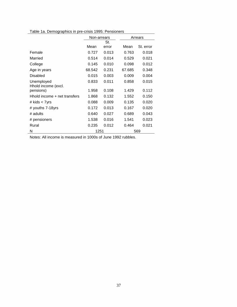
Tables 1a and 1b present summary statistics of our sample of pensioners and non-

pensioners in 1995, one year prior to the crisis. Over 70% of our pensioner sample is female

which reflects the much lower life expectancy of Russian men than women. Pensioners in arrears

are similar to those in non-arrears except for the former’s lower education, higher incidence of

unemployment, lower total household income (excluding pensions) and higher propensity to live

in rural areas. Among the non-pensioners living in pensioner households we observe similar

differences between the group living with pensioners in arrears and the group living with

pensioners in non-arrears. On average, the former group has lower levels of each of the

following characteristics: education, income (both personal and overall household income) and

urbanization of population center.

III. The pension crisis of 1996

The old-age pension system in Russia is administered by the state pension fund – the

Pension Fund of Russia (PFR) – which gives out monthly pensions to all individuals of

12

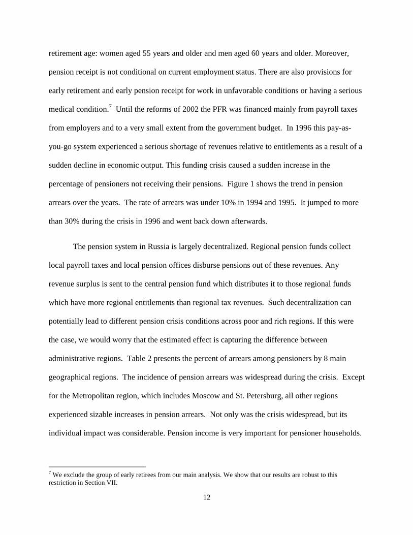
retirement age: women aged 55 years and older and men aged 60 years and older. Moreover,

pension receipt is not conditional on current employment status. There are also provisions for

early retirement and early pension receipt for work in unfavorable conditions or having a serious

medical condition.7 Until the reforms of 2002 the PFR was financed mainly from payroll taxes

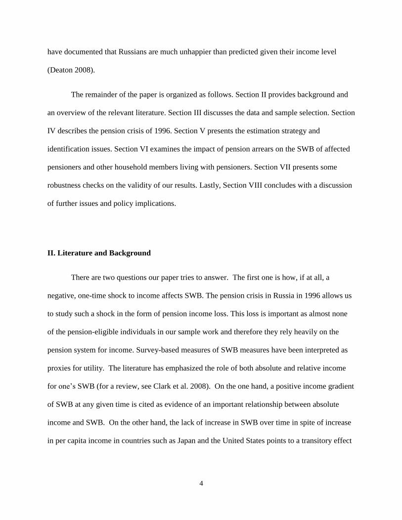
from employers and to a very small extent from the government budget. In 1996 this pay-as-

you-go system experienced a serious shortage of revenues relative to entitlements as a result of a

sudden decline in economic output. This funding crisis caused a sudden increase in the

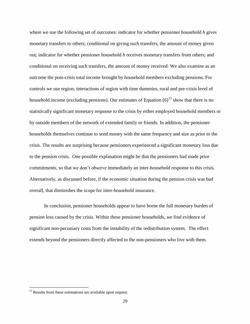
percentage of pensioners not receiving their pensions. Figure 1 shows the trend in pension

arrears over the years. The rate of arrears was under 10% in 1994 and 1995. It jumped to more

than 30% during the crisis in 1996 and went back down afterwards.

The pension system in Russia is largely decentralized. Regional pension funds collect

local payroll taxes and local pension offices disburse pensions out of these revenues. Any

revenue surplus is sent to the central pension fund which distributes it to those regional funds

which have more regional entitlements than regional tax revenues. Such decentralization can

potentially lead to different pension crisis conditions across poor and rich regions. If this were

the case, we would worry that the estimated effect is capturing the difference between

administrative regions. Table 2 presents the percent of arrears among pensioners by 8 main

geographical regions. The incidence of pension arrears was widespread during the crisis. Except

for the Metropolitan region, which includes Moscow and St. Petersburg, all other regions

experienced sizable increases in pension arrears. Not only was the crisis widespread, but its

individual impact was considerable. Pension income is very important for pensioner households.

7 We exclude the group of early retirees from our main analysis. We show that our results are robust to this

restriction in Section VII.

13

In 1995, pension income represented 57.6% of the total household income for pensioner

households in our RLMS sample.

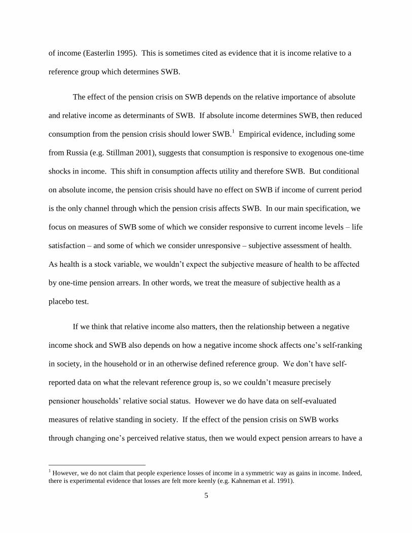
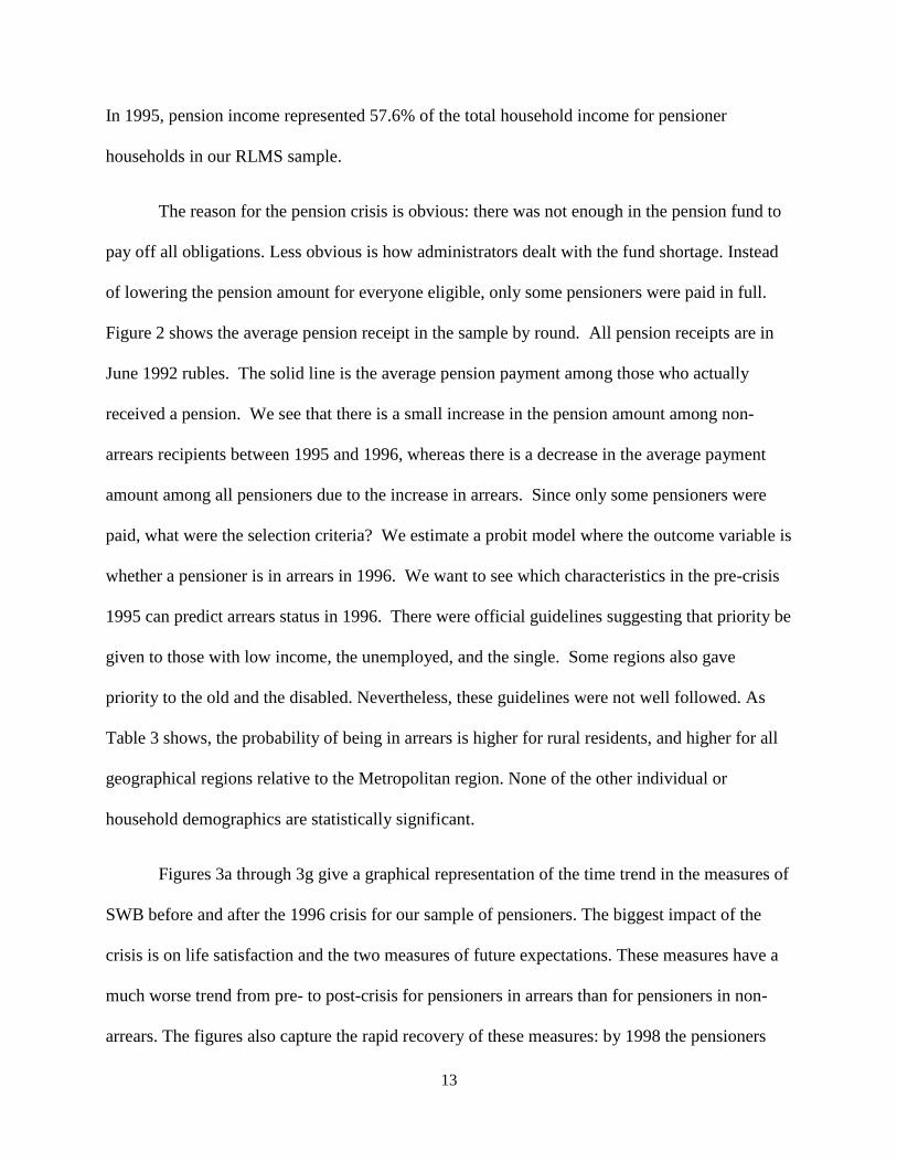
The reason for the pension crisis is obvious: there was not enough in the pension fund to

pay off all obligations. Less obvious is how administrators dealt with the fund shortage. Instead

of lowering the pension amount for everyone eligible, only some pensioners were paid in full.

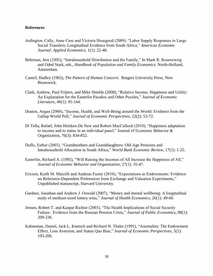
Figure 2 shows the average pension receipt in the sample by round. All pension receipts are in

June 1992 rubles. The solid line is the average pension payment among those who actually

received a pension. We see that there is a small increase in the pension amount among non-

arrears recipients between 1995 and 1996, whereas there is a decrease in the average payment

amount among all pensioners due to the increase in arrears. Since only some pensioners were

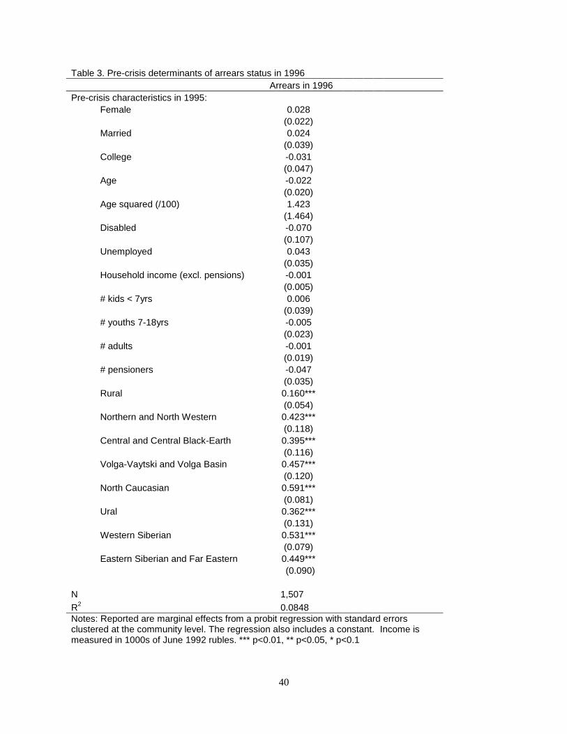
paid, what were the selection criteria? We estimate a probit model where the outcome variable is

whether a pensioner is in arrears in 1996. We want to see which characteristics in the pre-crisis

1995 can predict arrears status in 1996. There were official guidelines suggesting that priority be

given to those with low income, the unemployed, and the single. Some regions also gave

priority to the old and the disabled. Nevertheless, these guidelines were not well followed. As

Table 3 shows, the probability of being in arrears is higher for rural residents, and higher for all

geographical regions relative to the Metropolitan region. None of the other individual or

household demographics are statistically significant.

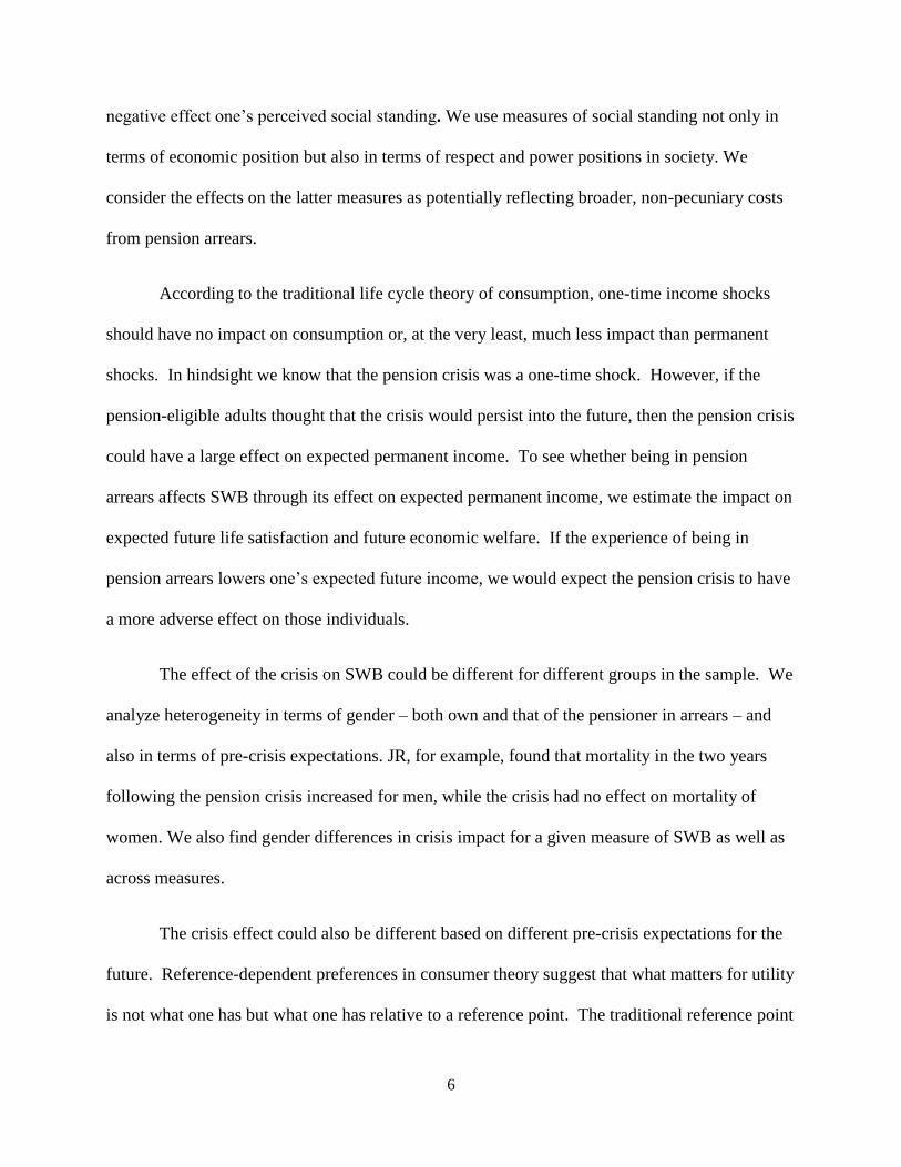
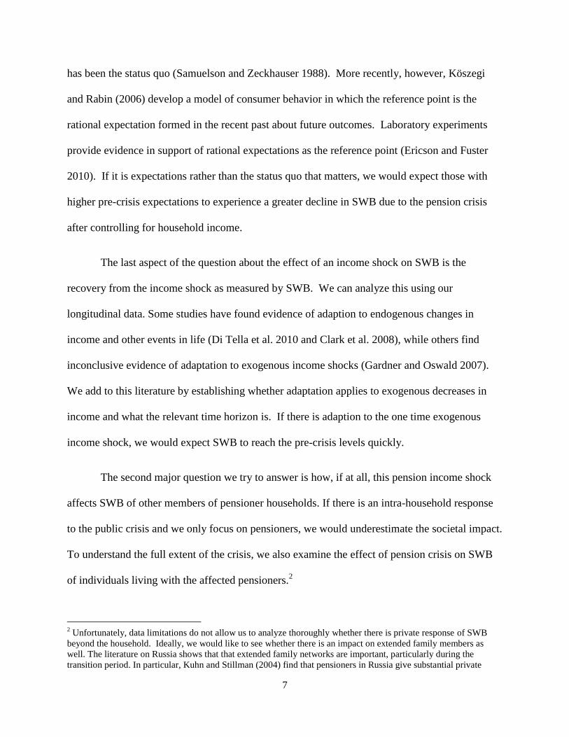
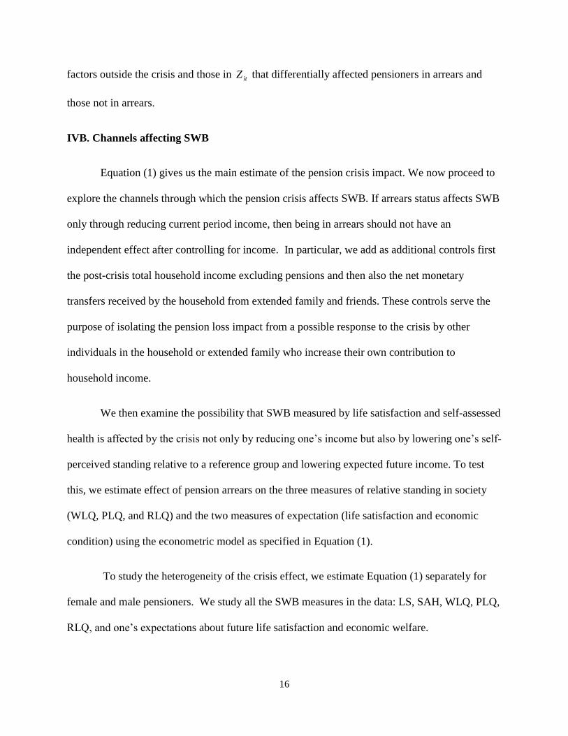
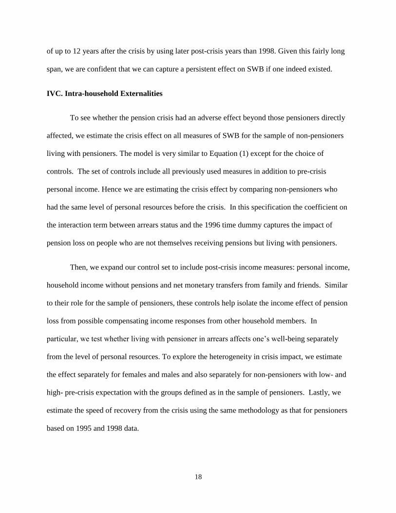
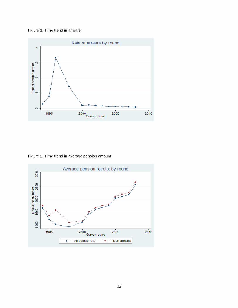
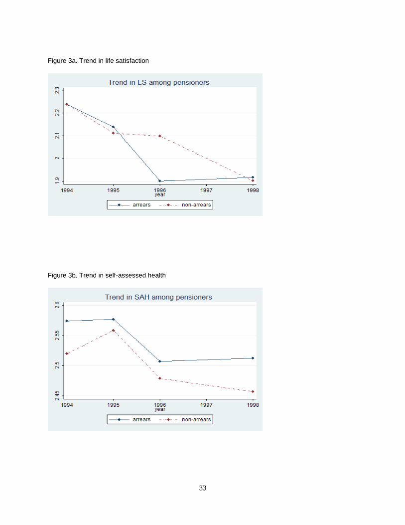
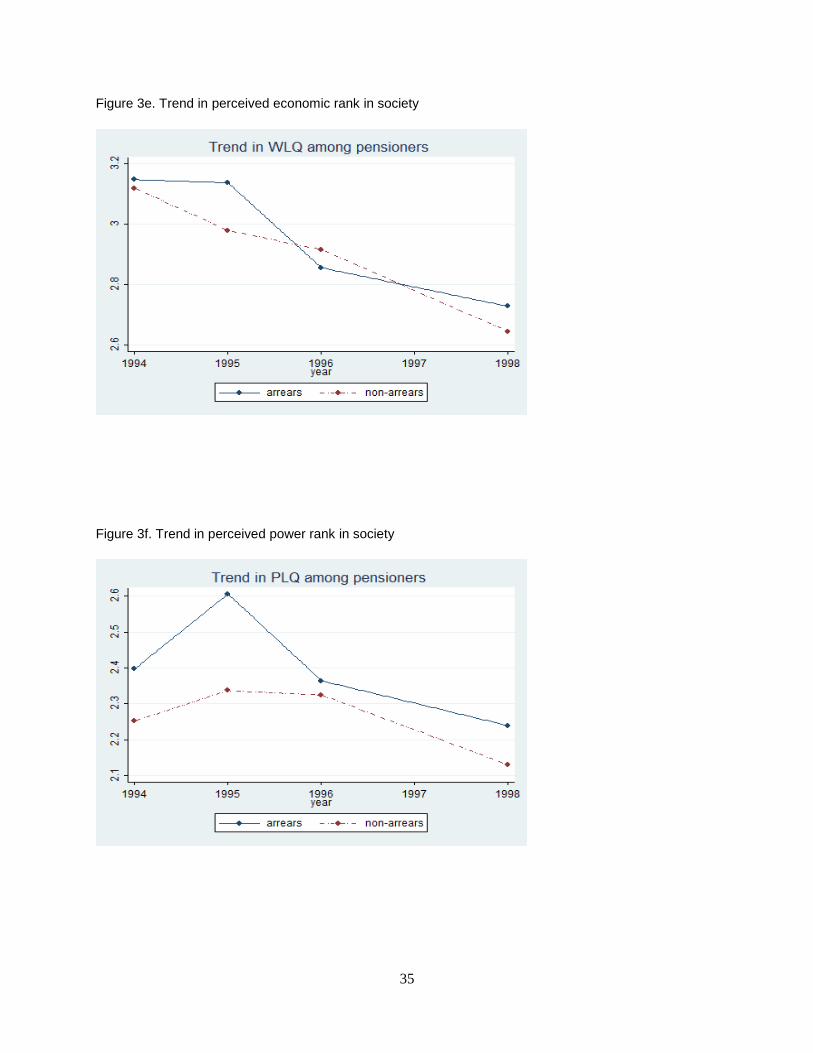
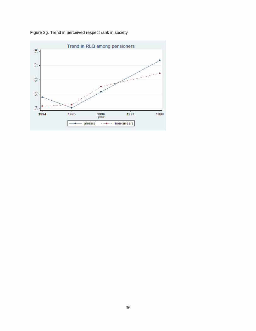
Figures 3a through 3g give a graphical representation of the time trend in the measures of

SWB before and after the 1996 crisis for our sample of pensioners. The biggest impact of the

crisis is on life satisfaction and the two measures of future expectations. These measures have a

much worse trend from pre- to post-crisis for pensioners in arrears than for pensioners in non-

arrears. The figures also capture the rapid recovery of these measures: by 1998 the pensioners

14

affected by the crisis report similar well-being as the pensioners who remained unscathed by the

crisis.

Next, we analyze these effects in a regression framework in order to investigate the

channels through which the crisis impacts SWB.

IV. Empirical Strategy

IVA. Main estimates

We employ a difference-in-difference (DD) approach to study the impact of pension

arrears on SWB. In particular, we compare the change in the measures of SWB before and after

the pension crisis for our treatment and control groups. In the pensioner sample, our treatment

group is those pensioners who did not receive their pensions as a result of the 1996 crisis (but

received it prior to the crisis) and our control group is those pensioners who received pensions in

both 1995 and 1996. In the sample of other individuals living with pensioners, but not

themselves pensioners, we define the treatment group as individuals living with pensioners in

arrears during the crisis and the control group as those living with pensioners not in arrears

during the crisis. The identifying assumption is that in the absence of the crisis, there would not

be differential trends in the measures of SWB between treatment and control groups.

The decentralized nature of the pension system implies the possibility of differential

impact across regions. In addition, the official guidelines that determined priority of pension

receipts could also induce differences between our treatment and control groups. Therefore, to

guard against such potential problems we control for such pre-crisis characteristics. Even if

15

treatment, i.e. arrears status, were randomly assigned, adding additional controls only improves

the efficiency of our estimates. Therefore, we estimate the following equation:

itittitiit ZYearArrearsYearArrearsy 1996*1996 3210 , (1)

where ity is the subjective well-being measure of individual i at time t (t = 1995, 1996),

iArrears is an indicator variable which equals 1 if the individual did not receive his/her pension

during the pension crisis of 1996, tYear1996 is an indicator variable for the year of the pension

crisis, and itZ is a vector of pre-crisis demographic and socio-economic characteristics, which

are likely to be correlated with arrears status as well as with SWB. These include dummy for

female, married, college degree, age, age squared, dummy for being disabled pre-crisis, dummy

for being unemployed pre-crisis, pre-crisis total household income8 excluding pensions, number

of household members in age groups 0-6, 7-17, number of adults in pre-pension age and number

of pensioners in the household, dummy for residing in rural area. We also include dummies for 8

major geographical regions (presented in Table 2) as well as their interactions with tYear1996 to

control for regional trends. We estimate Equation (1) as an ordered probit model and we cluster

the standard errors at the level of a census district.9 The coefficient of interest, 3 , gives the

impact of the pension crisis. Namely, it is the difference in the post-crisis change in SWB

between the treatment group (pensioners in arrears in 1996 or their household members) and the

control group (pensioners not in arrears or their household members who otherwise have the

same characteristics as the treatment group). Identification depends on there being no other

8 All income measures we use in subsequent analysis are converted to June 1992 rubles. In addition, top-coding

reported income at the 99 percentile leaves all our results unchanged. 9 As part of our robustness checks, we also estimate equation (1) using a linear probability model as well as a

different level of clustering of the standard errors. The qualitative results don’t change and are available upon

request.

16

factors outside the crisis and those in itZ that differentially affected pensioners in arrears and

those not in arrears.

IVB. Channels affecting SWB

Equation (1) gives us the main estimate of the pension crisis impact. We now proceed to

explore the channels through which the pension crisis affects SWB. If arrears status affects SWB

only through reducing current period income, then being in arrears should not have an

independent effect after controlling for income. In particular, we add as additional controls first

the post-crisis total household income excluding pensions and then also the net monetary

transfers received by the household from extended family and friends. These controls serve the

purpose of isolating the pension loss impact from a possible response to the crisis by other

individuals in the household or extended family who increase their own contribution to

household income.

We then examine the possibility that SWB measured by life satisfaction and self-assessed

health is affected by the crisis not only by reducing one’s income but also by lowering one’s self-

perceived standing relative to a reference group and lowering expected future income. To test

this, we estimate effect of pension arrears on the three measures of relative standing in society

(WLQ, PLQ, and RLQ) and the two measures of expectation (life satisfaction and economic

condition) using the econometric model as specified in Equation (1).

To study the heterogeneity of the crisis effect, we estimate Equation (1) separately for

female and male pensioners. We study all the SWB measures in the data: LS, SAH, WLQ, PLQ,

RLQ, and one’s expectations about future life satisfaction and economic welfare.

17

We also test the hypothesis that overall pre-crisis expectation is the reference point that

determines how the crisis impacts SWB. To do this we estimate Equation (1) separately for two

groups that differ in their pre-crisis expectation. The overall pre-crisis expectation is measured

in 1995, one year prior to the pension crisis. The outcomes of interests are LS, SAH, WLQ,

PLQ, and RLQ. In our data we have two measures of expectations, life satisfaction and

economic welfare, each defined on a 0 to 5 scale. We sum the two measures of expectations to

obtain one measure of overall expectation on a 0 to 10 scale. Those individuals with an overall

pre-crisis expectation measure of four or less are defined as having low pre-crisis outlook; and

those with an expectation measure greater than four are defined as having a high pre-crisis

outlook. We estimate Equation (1) separately for these two groups of low- and high-outlook

pensioners.

The last remaining aspect of the income-happiness question which we analyze is how fast

SWB adapts to the income shock after the crisis. In particular, we estimate the following

equation:

itititiit ZYearArrearsYearArrearsy 1998*1998 3210 (2)

where the subscript t indicates either the pre-crisis 1995 or the post-crisis 1998 which is the first

post-crisis year after 1996 in which the survey respondents were re-interviewed. Given this

specification, 3 captures the difference in the trend of SWB between treatment and control

groups over a period of 2 years after the crisis occurred. An estimate of this coefficient that is

statistically significant from 0 would indicate that the one-time crisis of 1996 had a persistent

effect on SWB. As our full data set extends to 2008, we can also use (2) to test for a persistency

18

of up to 12 years after the crisis by using later post-crisis years than 1998. Given this fairly long

span, we are confident that we can capture a persistent effect on SWB if one indeed existed.

IVC. Intra-household Externalities

To see whether the pension crisis had an adverse effect beyond those pensioners directly

affected, we estimate the crisis effect on all measures of SWB for the sample of non-pensioners

living with pensioners. The model is very similar to Equation (1) except for the choice of

controls. The set of controls include all previously used measures in addition to pre-crisis

personal income. Hence we are estimating the crisis effect by comparing non-pensioners who

had the same level of personal resources before the crisis. In this specification the coefficient on

the interaction term between arrears status and the 1996 time dummy captures the impact of

pension loss on people who are not themselves receiving pensions but living with pensioners.

Then, we expand our control set to include post-crisis income measures: personal income,

household income without pensions and net monetary transfers from family and friends. Similar

to their role for the sample of pensioners, these controls help isolate the income effect of pension

loss from possible compensating income responses from other household members. In

particular, we test whether living with pensioner in arrears affects one’s well-being separately

from the level of personal resources. To explore the heterogeneity in crisis impact, we estimate

the effect separately for females and males and also separately for non-pensioners with low- and

high- pre-crisis expectation with the groups defined as in the sample of pensioners. Lastly, we

estimate the speed of recovery from the crisis using the same methodology as that for pensioners

based on 1995 and 1998 data.

19

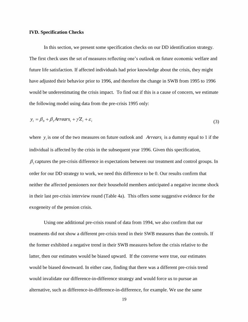
IVD. Specification Checks

In this section, we present some specification checks on our DD identification strategy.

The first check uses the set of measures reflecting one’s outlook on future economic welfare and

future life satisfaction. If affected individuals had prior knowledge about the crisis, they might

have adjusted their behavior prior to 1996, and therefore the change in SWB from 1995 to 1996

would be underestimating the crisis impact. To find out if this is a cause of concern, we estimate

the following model using data from the pre-crisis 1995 only:

iiii ZArrearsy 10 (3)

where iy is one of the two measures on future outlook and iArrears is a dummy equal to 1 if the

individual is affected by the crisis in the subsequent year 1996. Given this specification,

1 captures the pre-crisis difference in expectations between our treatment and control groups. In

order for our DD strategy to work, we need this difference to be 0. Our results confirm that

neither the affected pensioners nor their household members anticipated a negative income shock

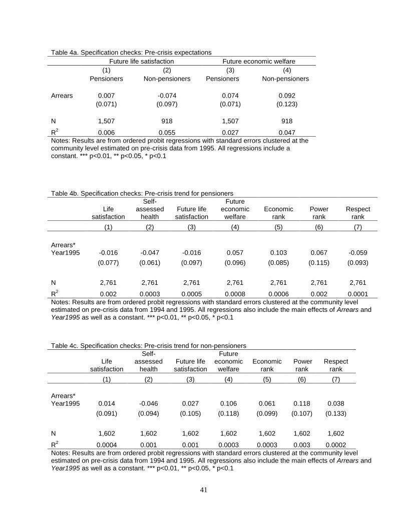
in their last pre-crisis interview round (Table 4a). This offers some suggestive evidence for the

exogeneity of the pension crisis.

Using one additional pre-crisis round of data from 1994, we also confirm that our

treatments did not show a different pre-crisis trend in their SWB measures than the controls. If

the former exhibited a negative trend in their SWB measures before the crisis relative to the

latter, then our estimates would be biased upward. If the converse were true, our estimates

would be biased downward. In either case, finding that there was a different pre-crisis trend

would invalidate our difference-in-difference strategy and would force us to pursue an

alternative, such as difference-in-difference-in-difference, for example. We use the same

20

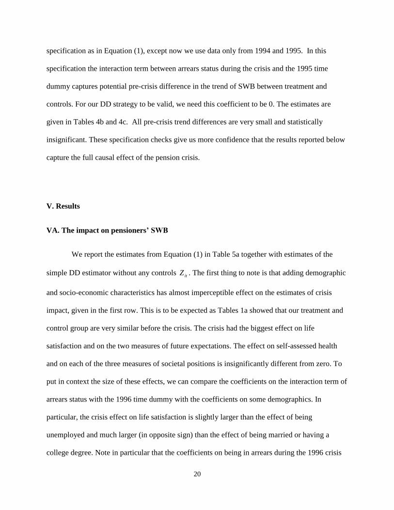
specification as in Equation (1), except now we use data only from 1994 and 1995. In this

specification the interaction term between arrears status during the crisis and the 1995 time

dummy captures potential pre-crisis difference in the trend of SWB between treatment and

controls. For our DD strategy to be valid, we need this coefficient to be 0. The estimates are

given in Tables 4b and 4c. All pre-crisis trend differences are very small and statistically

insignificant. These specification checks give us more confidence that the results reported below

capture the full causal effect of the pension crisis.

V. Results

VA. The impact on pensioners’ SWB

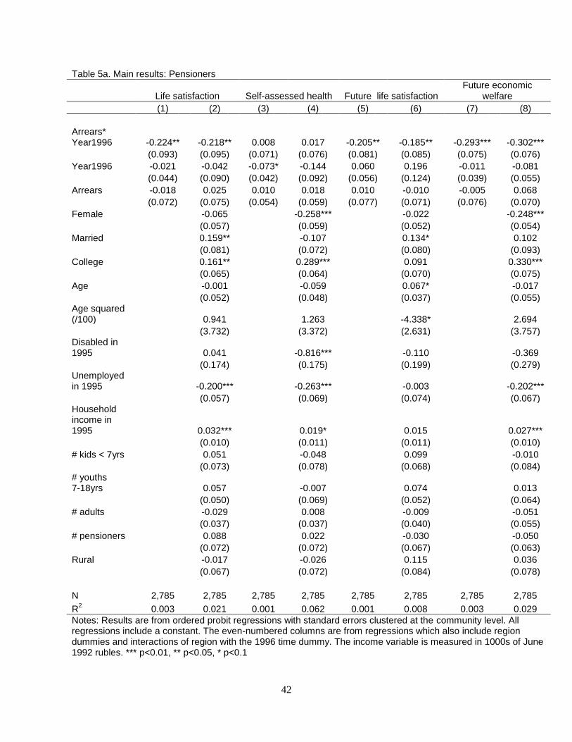
We report the estimates from Equation (1) in Table 5a together with estimates of the

simple DD estimator without any controls itZ . The first thing to note is that adding demographic

and socio-economic characteristics has almost imperceptible effect on the estimates of crisis

impact, given in the first row. This is to be expected as Tables 1a showed that our treatment and

control group are very similar before the crisis. The crisis had the biggest effect on life

satisfaction and on the two measures of future expectations. The effect on self-assessed health

and on each of the three measures of societal positions is insignificantly different from zero. To

put in context the size of these effects, we can compare the coefficients on the interaction term of

arrears status with the 1996 time dummy with the coefficients on some demographics. In

particular, the crisis effect on life satisfaction is slightly larger than the effect of being

unemployed and much larger (in opposite sign) than the effect of being married or having a

college degree. Note in particular that the coefficients on being in arrears during the 1996 crisis

21

are ten times as large in absolute value as the coefficients on household income. Household

income is measured in 1000s of June 1992 rubles and as Figure 2 shows, an average pension in

1995 was around 1300 June 1992 rubbles. Thus, the loss of around 1300 rubles in the pension

crisis appears to exert ten times as large an effect on well-being than a gain of 1000 rubles in

household income. We consider this suggestive evidence that the pension crisis had a very large

non-pecuniary cost for pensioners.

The finding of substantial effect on LS and no effect on SAH goes in line with our

understanding of the former being a flow quantity influenced by current levels of income, and

the latter being a stock quantity uninfluenced by current levels of income. More surprising is our

finding of a statistically insignificant effect on the pensioners’ self-perceived economic position

in society. One possible explanation for this is that there was widespread decline in economic

welfare during 1996 (as we describe earlier) and hence pensioners’ relative economic standing in

society was not influenced.

These results are robust to the inclusion of post-crisis income measures such as overall

household income (excluding pensions) and net transfers from extended family and friends. We

interpret the estimates in Table 6a as the effect of pension loss isolated from any earnings

response to the crisis by other household members or extended family. In fact, there is little

evidence of such response, as we discuss in Section VIII.

Tables 7a and 8a show that the crisis had a heterogeneous impact on well-being. Men

experience worsening in current well-being as reflected in the life satisfaction measure whereas

women are more concerned about the future as reflected in the two expectations measures. Pre-

crisis expectations, however, have smaller impact on how the crisis is experienced. Though not

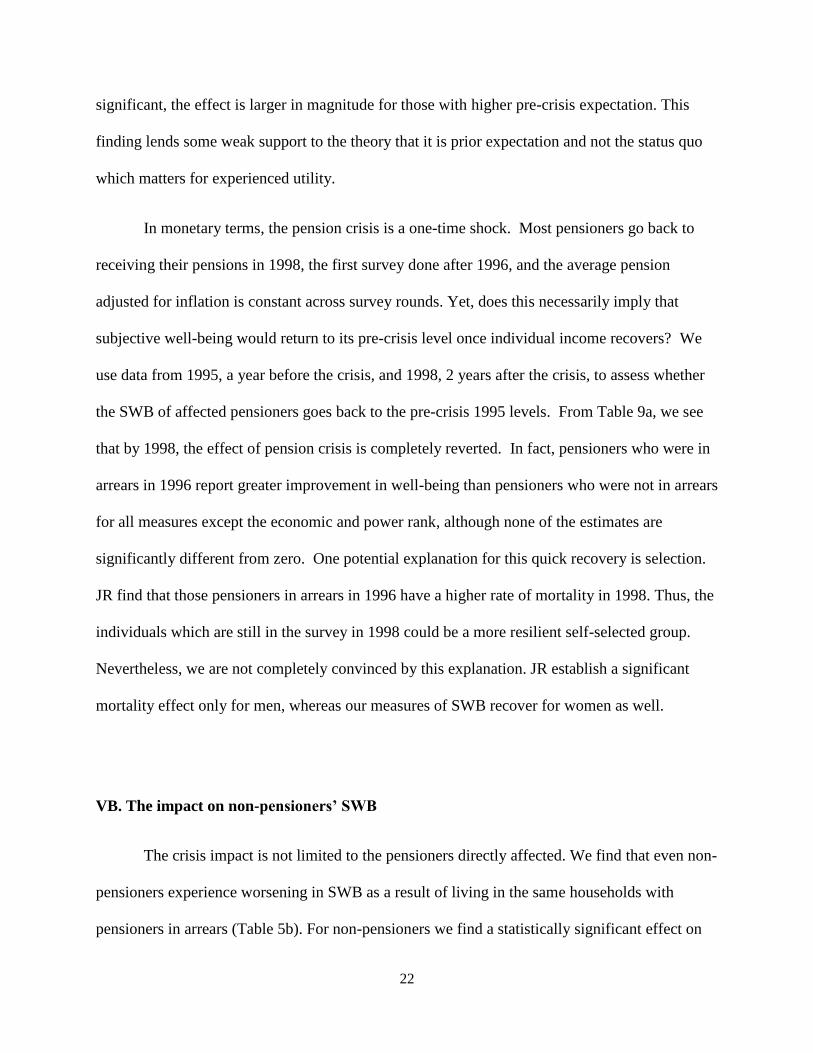
22

significant, the effect is larger in magnitude for those with higher pre-crisis expectation. This

finding lends some weak support to the theory that it is prior expectation and not the status quo

which matters for experienced utility.

In monetary terms, the pension crisis is a one-time shock. Most pensioners go back to

receiving their pensions in 1998, the first survey done after 1996, and the average pension

adjusted for inflation is constant across survey rounds. Yet, does this necessarily imply that

subjective well-being would return to its pre-crisis level once individual income recovers? We

use data from 1995, a year before the crisis, and 1998, 2 years after the crisis, to assess whether

the SWB of affected pensioners goes back to the pre-crisis 1995 levels. From Table 9a, we see

that by 1998, the effect of pension crisis is completely reverted. In fact, pensioners who were in

arrears in 1996 report greater improvement in well-being than pensioners who were not in arrears

for all measures except the economic and power rank, although none of the estimates are

significantly different from zero. One potential explanation for this quick recovery is selection.

JR find that those pensioners in arrears in 1996 have a higher rate of mortality in 1998. Thus, the

individuals which are still in the survey in 1998 could be a more resilient self-selected group.

Nevertheless, we are not completely convinced by this explanation. JR establish a significant

mortality effect only for men, whereas our measures of SWB recover for women as well.

VB. The impact on non-pensioners’ SWB

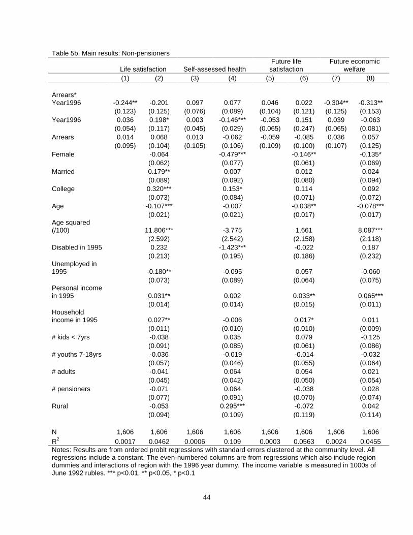
The crisis impact is not limited to the pensioners directly affected. We find that even non-

pensioners experience worsening in SWB as a result of living in the same households with

pensioners in arrears (Table 5b). For non-pensioners we find a statistically significant effect on

23

life satisfaction, expectation of future economic welfare and power and respect rankings. Out of

these, the well-being measures which are robust to the inclusion of pre-crisis demographic

controls are expectations of the future and societal rankings of power and respect. These effects

are equally strong (expectation of future economic welfare) or stronger (power and respect

ranking) than the effects on the pensioners directly affected. To put the size of these effects in

perspective, consider the effect on well-being from the demographic controls. For example,

living with an arrears pensioner during the crisis reduces one’s perceived power position in

society by as much as having a college degree increases it. This effect is larger than the effect of

being unemployed. Note in particular that the coefficients on both personal income and

household income are about ten times smaller in absolute value than the coefficients on being in

arrears in the 1996 crisis. This finding is the same as the one noted for pensioners. Like

pensioners, non-pensioners experience ten times as strongly a 1300-ruble loss in pension income

as a 1000-ruble gain in either personal or household income. We again note this as suggestive of

a strong non-pecuniary cost of the pension crisis.

Table 7b shows that these estimates are very robust to controls for post-crisis income

measures, including post-crisis personal income. We consider this suggestive evidence that the

crisis impact on non-pensioners can be at least partially attributed to non-pecuniary costs of

living with a pensioner in arrears.

The group of non-pensioners, similar to that of pensioners, shows heterogeneity in the

crisis impact. In particular, non-pensioners who had higher pre-crisis expectations are the ones

reporting a lower position in the societal ladder of power (Table 8b), which again is in

accordance to the theory of expectations being the reference point for experienced utility. The

effects also seem to be driven more by men than by women (Table 7b). These findings once

24

again confirm that the pensioner household cannot be perceived as a unit. Pensioners and non-

pensioners are impacted along different measures of subjective well-being and within those

categories women and men experience the crisis differently. We will go back to these results and

discuss their implications in Section VIII.

Lastly, we note that non-pensioners, like pensioners themselves, show a quick recovery

in their SWB (Table 9b). By 1998 none of the measures exhibit a significantly worse trend for

non-pensioners in arrears households than for non-pensioners in non-arrears households. In fact,

over 1995-1998 the former group see a higher relative improvement in their expectations about

future life satisfaction.

VII. Robustness checks

In this section we describe a series of robustness checks which establish that our results

are not sensitive to the specification we pick. All results are available upon request.

The first several robustness checks we perform are to test the assumptions underlying the

ordered probit specification. We re-estimate our main models using ordered logit and linear

probability specifications. We also recode each of our ordinal measures of SWB by collapsing

them into binary variables. For LS, SAH and the two measures of expectations, we recode as 1

all answers that are above 3 on the 0-5 scale. These answers, as described in the Data Section,

correspond to strictly positive reports of well-being or future expectations. For the three

measures of societal rank, we recode as 1 all answers above 4 on the 1-9 scale. This groups

together people who perceive their positions in society to be at the half-point mark or higher. All

these alternative specifications produce the same qualitative results as the original specification.

25

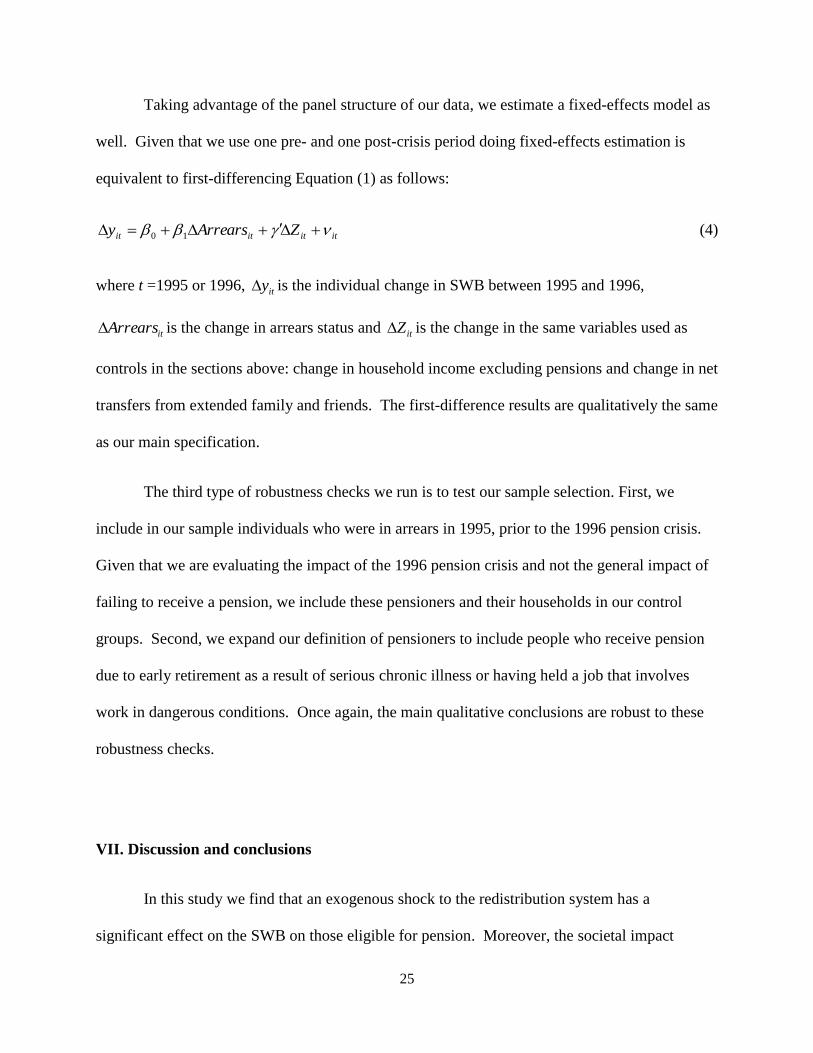
Taking advantage of the panel structure of our data, we estimate a fixed-effects model as

well. Given that we use one pre- and one post-crisis period doing fixed-effects estimation is

equivalent to first-differencing Equation (1) as follows:

itititit ZArrearsy 10 (4)

where t =1995 or 1996, ity is the individual change in SWB between 1995 and 1996,

itArrears is the change in arrears status and itZ is the change in the same variables used as

controls in the sections above: change in household income excluding pensions and change in net

transfers from extended family and friends. The first-difference results are qualitatively the same

as our main specification.

The third type of robustness checks we run is to test our sample selection. First, we

include in our sample individuals who were in arrears in 1995, prior to the 1996 pension crisis.

Given that we are evaluating the impact of the 1996 pension crisis and not the general impact of

failing to receive a pension, we include these pensioners and their households in our control

groups. Second, we expand our definition of pensioners to include people who receive pension

due to early retirement as a result of serious chronic illness or having held a job that involves

work in dangerous conditions. Once again, the main qualitative conclusions are robust to these

robustness checks.

VII. Discussion and conclusions

In this study we find that an exogenous shock to the redistribution system has a

significant effect on the SWB on those eligible for pension. Moreover, the societal impact

26

extends to non-pensioner members of these households. The reported decrease in well-being for

non-pensioners remains unchanged even after accounting for post-crisis personal income. In

addition, the crisis impact on non-pensioners is concentrated mostly on their self-perceived

positions of power and respect in society. One interpretation of these results is that the pension

crisis has a broader non-monetary effect on subjective well-being. Such an effect has been

documented for other life events such as unemployment (Luechinger et al. 2010). Indeed, we

estimate that pension arrears (experienced by oneself directly or by another household member)

causes decline in well-being of equal if not greater size than that of being unemployed.

Even more broadly, our results show that there are intra-household externalities in the

effects of the pension crisis. We believe that these results broadly fall within the growing debate

on the appropriate framework for modeling the household. For example, Lundberg et al. (2003)

find that among US households a man’s retirement status reduces his say in household

consumption decisions and so they argue that household resources are not shared equally among

household members. Our study contributes to this general debate on intra-household resource

allocation and to the specific question of how the pension loss is experienced within the

household.

The intra-household impact that we find could be partly due to preferences of the caring

type10

and partly due to income loss if pension income is shared among household members.

Two of the SWB measures, the economic rank one and expectations of future economic welfare,

however, should plausibly reflect only the economic impact of the crisis. As described before,

we consider the former measure to capture relative economic standing while the latter one – to

10

In the economic literature such preferences are described as follows: Ui= ui(xi) + u-i(x-i) where (0,1). In

other words, individual i’s utility or SWB depends not only on one’s own well-being but also on that of other

individuals -i where the extent of caring is captured by .

27

capture absolute economic position. If pension income is shared equally by all household

members regardless of who actually receives it, then there should be no difference in the impact

on the these economic measures between pensioners and non-pensioners. Thus, we could use our

results to perform a test of the unitary model. In particular, the unitary model implies that the

coefficient on the interaction term in equation (1) should be the same for the pensioner and non-

pensioner samples when we use as outcome self-perceived economic rank or expectations of

future welfare. As the estimates in Table 5a and 5b show, the coefficients are hardly different

and we cannot reject that either difference is statistically zero. Therefore, we fail to reject the

unitary model according to this formulation.

We found that the effect of pension arrears differs by gender for non-pensioners in

households with pensioners. It is also possible that the gender of the pensioners might affect the

impact of the pension crisis on non-pensioners. Another way to examine the intra-household

impact of the crisis is to establish whether the impact depends on the gender of the pensioner or

the number of pensioners in the household. To do this, we estimate the following equation:

(5)

where ijnArrears is an indicator variable for individual i which specifies whether i lives with n

number of pensioners of gender j, where n is 1 or 2, and j is female or male. The omitted

reference category is that there are no pensioners in the household who are in arrears. If the

household operates as a single unit, then the crisis impact should not depend on who the

pensioner is, i.e. we would expect mnfn for every n. In addition, we would expect the impact

itit

mfj n

ijnjnijnjntit ZYearArrearsArrearsYeary

)1996*(1996, 2,1

28

to increase with the number of pensioners, i.e. 0 21 jj for every j. 11

In general, our results

show that there is a somewhat differential impact with respect to the gender of the arrears

pensioner. The impact of having a pensioner in arrears is larger if the pensioner is female than if

the pensioner is male although the difference is not statistically significant.12

This suggestive

evidence is contrary to the assumptions of the unitary model. However, we don’t find this a

particularly conclusive test as it relies on the key assumption that female and male pensioner

households are the same. In the context of Russia with a very big gender difference in life

expectancy, we consider this assumption somewhat problematic. In future work, we plan to

investigate the structure of pensioner households by the gender of pensioner. Such analysis will

help to distinguish between heterogeneity due to the gender of pensioner and heterogeneity due

to sample selection.

Lastly, we test whether the crisis prompted a behavioral response of higher monetary

transfers to pensioners in arrears. We consider both an intra-household and an inter-household

response. The source of the former are employed adults living in the household who start bring

higher earnings. The source of the latter are extended family and friends who send more net

monetary transfers to pensioner households. Because those latter individuals are not part of the

survey we don’t have data on their SWB. However, we do have data on the transfers sent and

received by pensioner households. We estimate the equation below:

hthtththht ZYearArrearsYearArrearsy 1996*1996 3210 (6)

11

Unfortunately, in our sample we only observe households with at most 1 male pensioner in arrears and therefore

this particular test can be done only for the female pensioner coefficients when comparing n = 1,2 but can also be

done on male pensioner for the comparison of n = 1 versus the reference category of 0. 12

One possible explanation for this is that female pensioners share more of their pension with other household

members than male pensioners. Indeed, when we estimate the impact of the crisis on calories consumed, we find that

non-pensioners consume slightly fewer calories when they live with a female pensioner in arrears than when they

live with a male pensioner in arrears.

29

where we use the following set of outcomes: indicator for whether pensioner household h gives

monetary transfers to others; conditional on giving such transfers, the amount of money given

out; indicator for whether pensioner household h receives monetary transfers from others; and

conditional on receiving such transfers, the amount of money received. We also examine as an

outcome the post-crisis total income brought by household members excluding pensions. For

controls we use region, interactions of region with time dummies, rural and pre-crisis level of

household income (excluding pensions). Our estimates of Equation (6)13

show that there is no

statistically significant monetary response to the crisis by either employed household members or

by outside members of the network of extended family or friends. In addition, the pensioner

households themselves continue to send money with the same frequency and size as prior to the

crisis. The results are surprising because pensioners experienced a significant monetary loss due

to the pension crisis. One possible explanation might be that the pensioners had made prior

commitments, so that we don’t observe immediately an inter-household response to this crisis.

Alternatively, as discussed before, if the economic situation during the pension crisis was bad

overall, that diminishes the scope for inter-household insurance.

In conclusion, pensioner households appear to have borne the full monetary burden of

pension loss caused by the crisis. Within these pensioner households, we find evidence of

significant non-pecuniary costs from the instability of the redistribution system. The effect

extends beyond the pensioners directly affected to the non-pensioners who live with them.

13

Results from these estimations are available upon request.

30

References

Ardington, Cally, Anne Case and Victoria Hosegood (2009), “Labor Supply Responses to Large

Social Transfers: Longitudinal Evidence from South Africa,” American Economic

Journal: Applied Economics, 1(1): 22-48.

Behrman, Jere (1995), “Intrahousehold Distribution and the Family,” In Mark R. Rosenzweig

and Oded Stark, eds., Handbook of Population and Family Economics. North-Holland,

Amsterdam.

Cantril, Hadley (1965), The Pattern of Human Concern. Rutgers University Press, New

Brunswick.

Clark, Andrew, Paul Frijters, and Mike Shields (2008), “Relative Income, Happiness and Utility:

An Explanation for the Easterlin Paradox and Other Puzzles,” Journal of Economic

Literature, 46(1): 95-144.

Deaton, Angus (2008), “Income, Health, and Well-Being around the World: Evidence from the

Gallup World Poll,” Journal of Economic Perspectives, 22(2): 53-72.

Di Tella, Rafael, John Heisken-De New and Robert MacCulloch (2010), “Happiness adaptation

to income and to status in an individual panel,” Journal of Economic Behavior &

Organization, 76(3): 834-852.

Duflo, Esther (2003), “Grandmothers and Granddaughters: Old-Age Pensions and

Intrahousehold Allocation in South Africa,” World Bank Economic Review, 17(1): 1-25.

Easterlin, Richard A. (1995), “Will Raising the Incomes of All Increase the Happiness of All,”

Journal of Economic Behavior and Organization, 27(1): 35-47.

Ericson, Keith M. Marzilli and Andreas Fuster (2010), “Expectations as Endowments: Evidence

on Reference-Dependent Preferences from Exchange and Valuation Experiments,”

Unpublished manuscript, Harvard University.

Gardner, Jonathan and Andrew J. Oswald (2007), “Money and mental wellbeing: A longitudinal

study of medium-sized lottery wins,” Journal of Health Economics, 26(1): 49-60.

Jensen, Robert T. and Kaspar Richter (2003), “The Health Implications of Social Security

Failure: Evidence from the Russian Pension Crisis,” Journal of Public Economics, 88(1):

209-236.

Kahneman, Daniel, Jack L. Knetsch and Richard H. Thaler (1991), “Anomalies: The Endowment

Effect, Loss Aversion, and Status Quo Bias,” Journal of Economic Perspectives, 5(1):

193-206.

31

Koszegi, B. and M. Rabin (2006), “A Model of Reference-Dependent Preferences,” Quarterly

Journal of Economics, 121, 1133-1165.

Kuhn, Randall and Steven Stillman (2004), “Understanding Interhousehold Transfers in a

Transition Economy: Evidence from Russia,” Economic Development and Cultural

Change, 53(1): 131-156.

Lokshin, Michael and Martin Ravallion (2005), “Rich and Powerful? Subjective Power and

Welfare in Russia,” Journal of Economic Behavior and Organization, 56(2): 141-172.

Luechinger, Simon, Stephan Meier, and Alois Stutzer (2010), “Why Does Unemployment Hurt

the Employed? Evidence from the Life Satisfaction Gap between the Public and the

Private Sector,” Journal of Human Resources, 45(4): 998-1045.

Lundberg, Shelly, Richard Startz and Steven Stillman (2003), “The Retirement-Consumption

Puzzle: a Marital Bargaining Approach,” Journal of Public Economics, 87(5-6): 1199-

1218.

Samuelson, W. and R. Zeckhauser (1988), “Status quo bias in decision making," Journal of Risk

and Uncertainty, 1, 7-59.

Stillman, Steven (2001), “The Response of Consumption in Russian Households to Economic

Shocks,” IZA Discussion Paper 411, Bonn, Germany.

Stutzer, Alois and Bruno S. Frey (2010), “Recent Advances in the Economics of Individual

Subjective Well-Being,” Social Research, 77(2): 679-714.

32

Figure 1. Time trend in arrears

Figure 2. Time trend in average pension amount

33

Figure 3a. Trend in life satisfaction

Figure 3b. Trend in self-assessed health

34

Figure 3c. Trend in expected future economic welfare

Figure 3d. Trend in expected future life satisfaction

35

Figure 3e. Trend in perceived economic rank in society

Figure 3f. Trend in perceived power rank in society

36

Figure 3g. Trend in perceived respect rank in society

37

Table 1a. Demographics in pre-crisis 1995: Pensioners

Non-arrears

Arrears

Mean

St. error

Mean St. error

Female 0.727 0.013

0.763 0.018

Married 0.514 0.014

0.529 0.021

College 0.145 0.010

0.098 0.012

Age in years 68.542 0.231

67.685 0.348

Disabled 0.015 0.003

0.009 0.004

Unemployed 0.833 0.011

0.858 0.015 Hhold income (excl. pensions) 1.958 0.108

1.429 0.112

Hhold income + net transfers 1.868 0.132

1.552 0.150

# kids < 7yrs 0.088 0.009

0.135 0.020

# youths 7-18yrs 0.172 0.013

0.167 0.020

# adults 0.640 0.027

0.689 0.043

# pensioners 1.538 0.016

1.541 0.023

Rural 0.235 0.012

0.464 0.021

N 1251

569

Notes: All income is measured in 1000s of June 1992 rubbles.

38

Table 1b. Demographics in pre-crisis 1995: Non-pensioners

Non-arrears

Arrears

Mean

St. error

Mean

St. error

Female 0.450 0.020

0.392 0.028

Married 0.591 0.020

0.615 0.028

College 0.275 0.018

0.162 0.021

Age in years 36.707 0.527

35.879 0.748

Disabled 0.023 0.006

0.038 0.011

Unemployed 0.325 0.019

0.354 0.027

Personal income 2.151 0.122

1.528 0.129 Hhold income (excl. pensions) 5.096 0.236

3.421 0.216

Hhold income + net transfers 4.955 0.229

3.083 0.393

# kids < 7yrs 0.286 0.021

0.395 0.038

# youths 7-18yrs 0.487 0.028

0.494 0.043

# adults 2.083 0.043

2.115 0.056

# pensioners 1.220 0.017

1.258 0.026

Rural 0.167 0.015

0.465 0.028

N 604

314

Notes: All income is measured in 1000s of June 1992 rubbles.

39

Table 2. Regional distribution of arrears during the pension crisis of 1996

Mean Standard Deviation Frequency

Metropolitan: Moscow and St. Petersburg 0.048 0.214 147

Northern and North Western 0.380 0.488 92

Central and Central Black-Earth 0.287 0.453 401

Volga-Vaytski and Volga Basin 0.365 0.482 353

North Caucasian 0.533 0.500 259

Ural 0.304 0.461 194

Western Siberian 0.518 0.501 164

Eastern Siberian and Far Eastern 0.299 0.460 147

Overall 0.348 0.477 1757

40

Table 3. Pre-crisis determinants of arrears status in 1996 Arrears in 1996

Pre-crisis characteristics in 1995: Female 0.028

(0.022)

Married 0.024

(0.039)

College -0.031

(0.047)

Age -0.022

(0.020)

Age squared (/100) 1.423

(1.464)

Disabled -0.070

(0.107)

Unemployed 0.043

(0.035)

Household income (excl. pensions) -0.001

(0.005)

# kids < 7yrs 0.006

(0.039)

# youths 7-18yrs -0.005

(0.023)

# adults -0.001

(0.019)

# pensioners -0.047

(0.035)

Rural 0.160***

(0.054)

Northern and North Western 0.423***

(0.118)

Central and Central Black-Earth 0.395***

(0.116)

Volga-Vaytski and Volga Basin 0.457***

(0.120)

North Caucasian 0.591***

(0.081)

Ural 0.362***

(0.131)

Western Siberian 0.531***

(0.079)

Eastern Siberian and Far Eastern 0.449***

(0.090)

N 1,507 R

2 0.0848

Notes: Reported are marginal effects from a probit regression with standard errors clustered at the community level. The regression also includes a constant. Income is measured in 1000s of June 1992 rubles. *** p<0.01, ** p<0.05, * p<0.1

41

Table 4a. Specification checks: Pre-crisis expectations Future life satisfaction Future economic welfare

(1) (2) (3) (4)

Pensioners Non-pensioners Pensioners Non-pensioners

Arrears 0.007 -0.074 0.074 0.092

(0.071) (0.097) (0.071) (0.123)

N 1,507 918 1,507 918

R2 0.006 0.055 0.027 0.047

Notes: Results are from ordered probit regressions with standard errors clustered at the community level estimated on pre-crisis data from 1995. All regressions include a constant. *** p<0.01, ** p<0.05, * p<0.1

Table 4b. Specification checks: Pre-crisis trend for pensioners

Life

satisfaction

Self-assessed

health Future life satisfaction

Future economic welfare

Economic rank

Power rank

Respect rank

(1) (2) (3) (4) (5) (6) (7)

Arrears* Year1995 -0.016 -0.047 -0.016 0.057 0.103 0.067 -0.059

(0.077) (0.061) (0.097) (0.096) (0.085) (0.115) (0.093)

N 2,761 2,761 2,761 2,761 2,761 2,761 2,761

R2 0.002 0.0003 0.0005 0.0008 0.0006 0.002 0.0001

Notes: Results are from ordered probit regressions with standard errors clustered at the community level estimated on pre-crisis data from 1994 and 1995. All regressions also include the main effects of Arrears and Year1995 as well as a constant. *** p<0.01, ** p<0.05, * p<0.1

Table 4c. Specification checks: Pre-crisis trend for non-pensioners

Life

satisfaction

Self-assessed



Economic rank

Power rank

Respect rank

(1) (2) (3) (4) (5) (6) (7)

Arrears* Year1995 0.014 -0.046 0.027 0.106 0.061 0.118 0.038

(0.091) (0.094) (0.105) (0.118) (0.099) (0.107) (0.133)

N 1,602 1,602 1,602 1,602 1,602 1,602 1,602

R2 0.0004 0.001 0.001 0.0003 0.0003 0.003 0.0002

Notes: Results are from ordered probit regressions with standard errors clustered at the community level estimated on pre-crisis data from 1994 and 1995. All regressions also include the main effects of Arrears and Year1995 as well as a constant. *** p<0.01, ** p<0.05, * p<0.1

42

Table 5a. Main results: Pensioners

Life satisfaction Self-assessed health Future life satisfaction Future economic

welfare

(1) (2) (3) (4) (5) (6) (7) (8)

Arrears* Year1996 -0.224** -0.218** 0.008 0.017 -0.205** -0.185** -0.293*** -0.302***

(0.093) (0.095) (0.071) (0.076) (0.081) (0.085) (0.075) (0.076)

Year1996 -0.021 -0.042 -0.073* -0.144 0.060 0.196 -0.011 -0.081

(0.044) (0.090) (0.042) (0.092) (0.056) (0.124) (0.039) (0.055)

Arrears -0.018 0.025 0.010 0.018 0.010 -0.010 -0.005 0.068

(0.072) (0.075) (0.054) (0.059) (0.077) (0.071) (0.076) (0.070)

Female

-0.065

-0.258***

-0.022

-0.248***

(0.057)

(0.059)

(0.052)

(0.054)

Married

0.159**

-0.107

0.134*

0.102

(0.081)

(0.072)

(0.080)

(0.093)

College

0.161**

0.289***

0.091

0.330***

(0.065)

(0.064)

(0.070)

(0.075)

Age

-0.001

-0.059

0.067*

-0.017

(0.052)

(0.048)

(0.037)

(0.055)

Age squared (/100)

0.941

1.263

-4.338*

2.694

(3.732)

(3.372)

(2.631)

(3.757)

Disabled in 1995

0.041

-0.816***

-0.110

-0.369

(0.174)

(0.175)

(0.199)

(0.279)

Unemployed in 1995

-0.200***

-0.263***

-0.003

-0.202***

(0.057)

(0.069)

(0.074)

(0.067)

Household income in 1995

0.032***

0.019*

0.015

0.027***

(0.010)

(0.011)

(0.011)

(0.010)

# kids < 7yrs

0.051

-0.048

0.099

-0.010

(0.073)

(0.078)

(0.068)

(0.084)

# youths 7-18yrs

0.057

-0.007

0.074

0.013

(0.050)

(0.069)

(0.052)

(0.064)

# adults

-0.029

0.008

-0.009

-0.051

(0.037)

(0.037)

(0.040)

(0.055)

# pensioners

0.088

0.022

-0.030

-0.050

(0.072)

(0.072)

(0.067)

(0.063)

Rural

-0.017

-0.026

0.115

0.036

(0.067)

(0.072)

(0.084)

(0.078)

N 2,785 2,785 2,785 2,785 2,785 2,785 2,785 2,785

R2 0.003 0.021 0.001 0.062 0.001 0.008 0.003 0.029

Notes: Results are from ordered probit regressions with standard errors clustered at the community level. All regressions include a constant. The even-numbered columns are from regressions which also include region dummies and interactions of region with the 1996 time dummy. The income variable is measured in 1000s of June 1992 rubles. *** p<0.01, ** p<0.05, * p<0.1

43

Table 5a. Main results: Pensioners (continued) Economic rank Power rank Respect rank

(9) (10) (11) (12) (13) (14)

Arrears*Year1996 -0.146* -0.130 -0.165* -0.153 -0.090 -0.042

(0.083) (0.088) (0.089) (0.095) (0.073) (0.075)

Year1996 -0.008 0.048 0.014 0.142*** 0.075 0.306**

(0.051) (0.069) (0.051) (0.034) (0.053) (0.128)

Arrears 0.083 0.071 0.176** 0.164** 0.013 -0.008

(0.089) (0.081) (0.084) (0.079) (0.072) (0.066)

Female

-0.061

0.009

-0.020

(0.049)

(0.054)

(0.042)

Married

0.258***

0.140**

0.118*

(0.079)

(0.069)

(0.069)

College

0.314***

0.248***

0.255***

(0.068)

(0.077)

(0.091)

Age

-0.021

-0.028

-0.023

(0.051)

(0.050)

(0.045)

Age squared (/100)

2.083

2.159

1.243

(3.625)

(3.475)

(3.227)

Disabled in 1995

-0.132

0.136

-0.039

(0.203)

(0.210)

(0.183)

Unemployed in 1995

-0.196***

-0.212***

-0.093

(0.067)

(0.075)

(0.061)


0.037***

0.001

0.015

(0.011)

(0.009)

(0.012)

# kids < 7yrs

-0.013

0.000

0.114

(0.075)

(0.091)

(0.074)

# youths 7-18yrs

0.121***

0.057

0.094*

(0.046)

(0.048)

(0.054)

# adults

-0.031

0.049

-0.058

(0.032)

(0.034)

(0.038)

# pensioners

0.070

0.013

-0.054

(0.060)

(0.059)

(0.069)

Rural

0.145*

0.175*

-0.072

(0.080)

(0.095)

(0.083)

N 2,785 2,785 2,785 2,785 2,785 2,785

R2 0.001 0.026 0.001 0.0140 0.0003 0.015

Notes: Results are from ordered probit regressions with standard errors clustered at the community level. All regressions include a constant. The even-numbered columns are from regressions which also include region dummies and interactions of region with the 1996 year dummy. The income variable is measured in 1000s of June 1992 rubles. *** p<0.01, ** p<0.05, * p<0.1

44

Table 5b. Main results: Non-pensioners

Life satisfaction Self-assessed health Future life satisfaction


(1) (2) (3) (4) (5) (6) (7) (8)

Arrears* Year1996 -0.244** -0.201 0.097 0.077 0.046 0.022 -0.304** -0.313**

(0.123) (0.125) (0.076) (0.089) (0.104) (0.121) (0.125) (0.153)

Year1996 0.036 0.198* 0.003 -0.146*** -0.053 0.151 0.039 -0.063

(0.054) (0.117) (0.045) (0.029) (0.065) (0.247) (0.065) (0.081)

Arrears 0.014 0.068 0.013 -0.062 -0.059 -0.085 0.036 0.057

(0.095) (0.104) (0.105) (0.106) (0.109) (0.100) (0.107) (0.125)

Female

-0.064

-0.479***

-0.146**

-0.135*

(0.062)

(0.077)

(0.061)

(0.069)

Married

0.179**

0.007

0.012

0.024

(0.089)

(0.092)

(0.080)

(0.094)

College

0.320***

0.153*

0.114

0.092

(0.073)

(0.084)

(0.071)

(0.072)

Age

-0.107***

-0.007

-0.038**

-0.078***

(0.021)

(0.021)

(0.017)

(0.017)

Age squared (/100)

11.806***

-3.775

1.661

8.087***

(2.592)

(2.542)

(2.158)

(2.118)

Disabled in 1995

0.232

-1.423***

-0.022

0.187

(0.213)

(0.195)

(0.186)

(0.232)

Unemployed in 1995

-0.180**

-0.095

0.057

-0.060

(0.073)

(0.089)

(0.064)

(0.075)

Personal income in 1995

0.031**

0.002

0.033**

0.065***

(0.014)

(0.014)

(0.015)

(0.011)


0.027**

-0.006

0.017*

0.011

(0.011)

(0.010)

(0.010)

(0.009)

# kids < 7yrs

-0.038

0.035

0.079

-0.125

(0.091)

(0.085)

(0.061)

(0.086)

# youths 7-18yrs

-0.036

-0.019

-0.014

-0.032

(0.057)

(0.046)

(0.055)

(0.064)

# adults

-0.041

0.064

0.054

0.021

(0.045)

(0.042)

(0.050)

(0.054)

# pensioners

-0.071

0.064

-0.038

0.028

(0.077)

(0.091)

(0.070)

(0.074)

Rural

-0.053

0.295***

-0.072

0.042

(0.094)

(0.109)

(0.119)

(0.114)

N 1,606 1,606 1,606 1,606 1,606 1,606 1,606 1,606

R2 0.0017 0.0462 0.0006 0.109 0.0003 0.0563 0.0024 0.0455


45

Table 5b. Main results: Non-pensioners (continued)

Economic rank Power rank Respect rank

(9) (10) (11) (12) (13) (14)

Arrears*Year1996 -0.148 -0.142 -

0.284*** -0.213** -0.234** -0.227*

(0.094) (0.098) (0.097) (0.106) (0.109) (0.121)

Year1996 0.051 0.279 0.157** 0.382** 0.072 0.296*

(0.057) (0.262) (0.062) (0.150) (0.064) (0.169)

Arrears 0.084 0.058 0.225** 0.135 0.034 -0.033

(0.085) (0.087) (0.103) (0.101) (0.098) (0.099)

Female

-0.003

-0.088

0.020

(0.054)

(0.060)

(0.055)

Married

0.086

0.101

0.037

(0.080)

(0.078)

(0.068)

College

0.162**

0.285***

0.107

(0.076)

(0.076)

(0.076)

Age

-0.086***

-0.055***

-0.024

(0.016)

(0.017)

(0.016)

Age squared (/100)

9.547***

5.142**

3.346

(2.026)

(2.244)

(2.047)

Disabled in 1995

-0.295*

-0.140

-0.163

(0.176)

(0.164)

(0.245)

Unemployed in 1995

-0.156**

-0.169**

-0.247***

(0.068)

(0.077)

(0.079)

Personal income in 1995

0.063***

0.029**

0.022*

(0.013)

(0.014)

(0.012)


0.020**

0.000

0.025***

(0.009)

(0.007)

(0.009)

# kids < 7yrs

-0.047

-0.104

0.002

(0.076)

(0.075)

(0.068)

# youths 7-18yrs

0.013

0.019

-0.012

(0.064)

(0.062)

(0.045)

# adults

0.054

0.056

-0.024

(0.039)

(0.037)

(0.032)

# pensioners

0.083

0.027

0.011

(0.076)

(0.066)

(0.074)

Rural

0.132

0.185*

0.091

(0.084)

(0.099)

(0.085)

N 1,606 1,606 1,606 1,606 1,606 1,606

R2 0.0003 0.0361 0.00202 0.0231 0.0010 0.0235


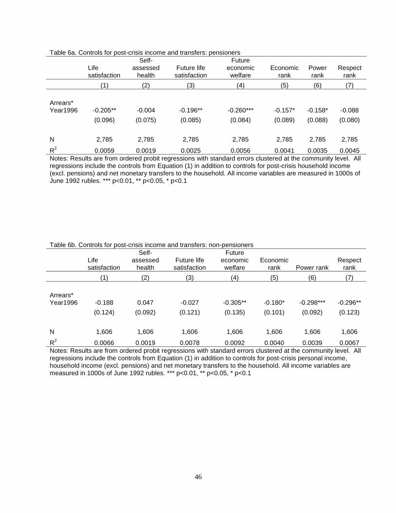
46

Table 6a. Controls for post-crisis income and transfers: pensioners

Life satisfaction

Self-assessed



Economic rank

Power rank

Respect rank

(1) (2) (3) (4) (5) (6) (7)

Arrears* Year1996 -0.205** -0.004 -0.196** -0.260*** -0.157* -0.158* -0.088

(0.096) (0.075) (0.085) (0.084) (0.089) (0.088) (0.080)

N 2,785 2,785 2,785 2,785 2,785 2,785 2,785

R2 0.0059 0.0019 0.0025 0.0056 0.0041 0.0035 0.0045

Notes: Results are from ordered probit regressions with standard errors clustered at the community level. All regressions include the controls from Equation (1) in addition to controls for post-crisis household income (excl. pensions) and net monetary transfers to the household. All income variables are measured in 1000s of June 1992 rubles. *** p<0.01, ** p<0.05, * p<0.1

Table 6b. Controls for post-crisis income and transfers: non-pensioners

Life satisfaction

Self-assessed

health Future life

satisfaction


Economic rank Power rank

Respect rank

(1) (2) (3) (4) (5) (6) (7)

Arrears* Year1996 -0.188 0.047 -0.027 -0.305** -0.180* -0.298*** -0.296**

(0.124) (0.092) (0.121) (0.135) (0.101) (0.092) (0.123)

N 1,606 1,606 1,606 1,606 1,606 1,606 1,606

R2 0.0066 0.0019 0.0078 0.0092 0.0040 0.0039 0.0067

Notes: Results are from ordered probit regressions with standard errors clustered at the community level. All regressions include the controls from Equation (1) in addition to controls for post-crisis personal income, household income (excl. pensions) and net monetary transfers to the household. All income variables are measured in 1000s of June 1992 rubles. *** p<0.01, ** p<0.05, * p<0.1

47

Table 7a. Effect of gender: pensioners

Life satisfaction Self-assessed health Future life satisfaction Future economic

welfare

(1) (2) (3) (4) (5) (6) (7) (8)

Men Women Men Women Men Women Men Women

Arrears* Year1996 -0.356** -0.162 -0.110 0.061 -0.068 -0.235*** -0.247 -0.318***

(0.164) (0.113) (0.136) (0.081) (0.167) (0.091) (0.159) (0.087)

N 767 2,018 767 2,018 767 2,018 767 2,018

R2 0.0341 0.0187 0.0594 0.0685 0.0268 0.0077 0.0388 0.0232

Notes: Results are from ordered probit regressions with standard errors clustered at the community level. All regressions include the controls from Equation (1). *** p<0.01, ** p<0.05, * p<0.1

Table 7a. Effect of gender: pensioners (continued)


(9) (10) (11) (12) (13) (14)

Men Women Men Women Men Women

Arrears*Year1996 -0.329* -0.066 -0.430*** -0.051 -0.139 -0.001

(0.174) (0.085) (0.141) (0.110) (0.148) (0.086)

N 767 2,018 767 2,018 767 2,018

R2 0.0330 0.0263 0.0320 0.0130 0.0183 0.0153


48

Table 7b. Effect of gender: non-pensioners

Life satisfaction Self-assessed

health Future life

satisfaction Future economic

welfare

(1) (2) (3) (4) (5) (6) (7) (8)

Men Women Men Women Men Women Men Women

Arrears* Year1996 -0.117 -0.347* 0.120 -0.018 0.041 -0.053 -0.387** -0.238

(0.153) (0.179) (0.113) (0.147) (0.151) (0.155) (0.171) (0.246)

N 910 696 910 696 910 696 910 696

R2 0.0582 0.0467 0.143 0.0933 0.0774 0.0429 0.0505 0.0566


Table 7b. Effect of gender: non-pensioners (continued)


(9) (10) (11) (12) (13) (14)

Men Women Men Women Men Women

Arrears* Year1996 -0.165 -0.141 -0.296** -0.154 -0.194 -0.262

(0.130) (0.151) (0.126) (0.160) (0.134) (0.186)

N 910 696 910 696 910 696

R2 0.0508 0.0342 0.0363 0.0190 0.0346 0.0216


49

Table 8a. Effect of pre-crisis expectations: pensioners

Life satisfaction Self-assessed health

(1) (2) (3) (4)

Low outlook High outlook Low outlook High outlook

Arrears* Year1996 -0.200 -0.269* 0.126 -0.211

(0.128) (0.144) (0.081) (0.138)

N 1,819 966 1,819 966

R2 0.0163 0.0403 0.0652 0.0712


Table 8a. Effect of pre-crisis expectations: pensioners (continued) Economic rank Power rank Respect rank

(5) (6) (7) (8) (9) (10)

Low outlook

High outlook

Low outlook

High outlook

Low outlook

High outlook

Arrears* Year1996 -0.085 -0.237 -0.086 -0.293* -0.047 -0.061

(0.100) (0.161) (0.097) (0.161) (0.099) (0.114)

N 1,819 966 1,819 966 1,819 966

R2 0.0290 0.0294 0.0156 0.0260 0.0187 0.0193


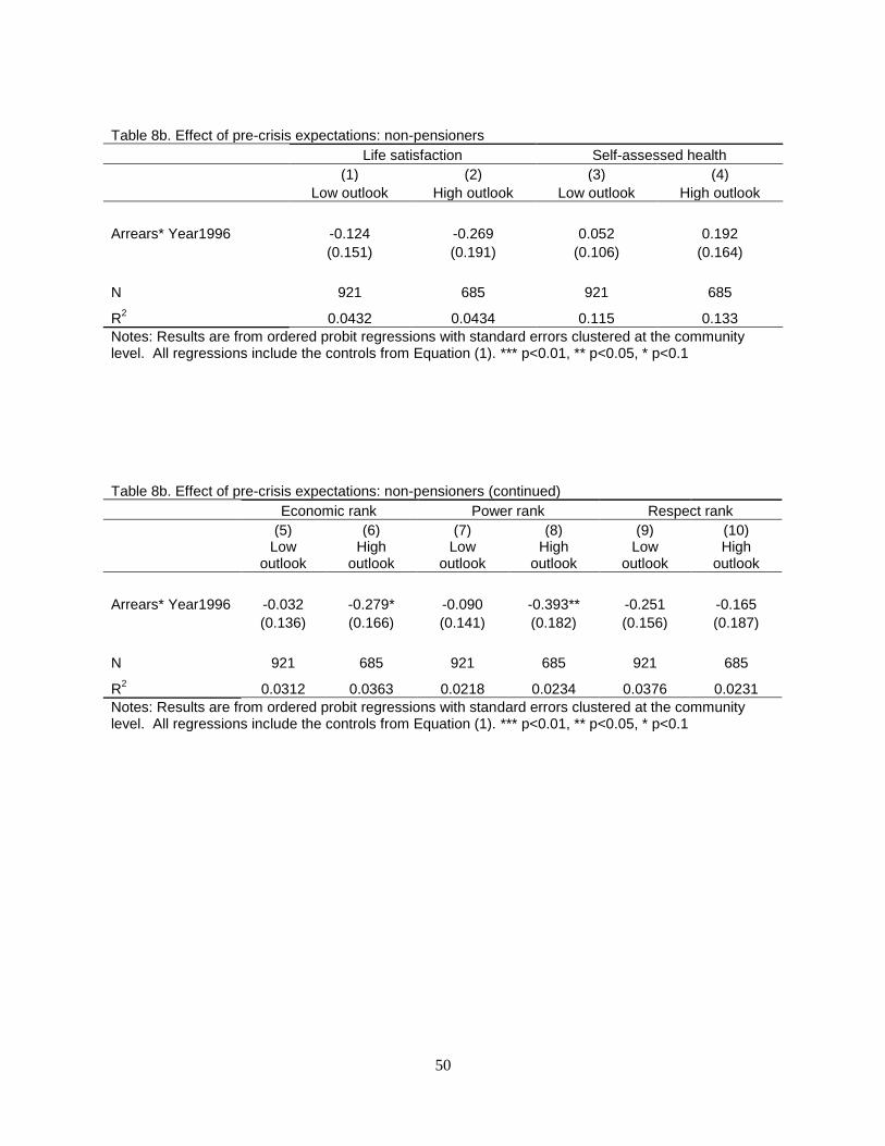
50

Table 8b. Effect of pre-crisis expectations: non-pensioners

Life satisfaction Self-assessed health

(1) (2) (3) (4)

Low outlook High outlook Low outlook High outlook

Arrears* Year1996 -0.124 -0.269 0.052 0.192

(0.151) (0.191) (0.106) (0.164)

N 921 685 921 685

R2 0.0432 0.0434 0.115 0.133


Table 8b. Effect of pre-crisis expectations: non-pensioners (continued) Economic rank Power rank Respect rank

(5) (6) (7) (8) (9) (10)

Low outlook

High outlook

Low outlook

High outlook

Low outlook

High outlook

Arrears* Year1996 -0.032 -0.279* -0.090 -0.393** -0.251 -0.165

(0.136) (0.166) (0.141) (0.182) (0.156) (0.187)

N 921 685 921 685 921 685

R2 0.0312 0.0363 0.0218 0.0234 0.0376 0.0231


51

Table 9a. Duration of crisis effect: pensioners

Life satisfaction

Self-assessed



Economic rank

Power rank

Respect rank

(1) (2) (3) (4) (5) (6) (7)

Arrears* Year1998 0.126 0.101 0.093 0.063 -0.004 -0.075 0.007

(0.098) (0.080) (0.097) (0.099) (0.090) (0.104) (0.093)

N 2,496 2,496 2,496 2,496 2,496 2,496 2,496

R2 0.0215 0.0770 0.0157 0.0404 0.0326 0.0178 0.0165

Notes: Results are from ordered probit regressions with standard errors clustered at the community level estimated on data from 1995 and 1998. All regressions include the controls from Equation (1). *** p<0.01, ** p<0.05, * p<0.1

Table 9b. Duration of crisis effect: non-pensioners

Life satisfaction

Self-assessed



Economic rank

Power rank

Respect rank

(1) (2) (3) (4) (5) (6) (7)

Arrears* Year1998 -0.102 -0.051 0.362** 0.134 -0.043 -0.150 -0.028

(0.135) (0.128) (0.146) (0.169) (0.134) (0.109) (0.153)

N 1,482 1,482 1,482 1,482 1,482 1,482 1,482

R2 0.0472 0.116 0.0666 0.0455 0.0364 0.0262 0.0228

Notes: Results are from ordered probit regressions with standard errors clustered at the community level estimated on data from 1995 and 1998. All regressions include the controls from Equation (1). *** p<0.01, ** p<0.05, * p<0.1

Documents

The Mental Cost of Pension Loss: The Experience of … Preliminary draft: Please do not cite The Mental Cost of Pension Loss: The Experience of Russia’s Pensioners during Transition