HAL Id: hal-00694764https://hal.archives-ouvertes.fr/hal-00694764

Submitted on 6 May 2012

HAL is a multi-disciplinary open accessarchive for the deposit and dissemination of sci-entific research documents, whether they are pub-lished or not. The documents may come fromteaching and research institutions in France orabroad, or from public or private research centers.

L’archive ouverte pluridisciplinaire HAL, estdestinée au dépôt et à la diffusion de documentsscientifiques de niveau recherche, publiés ou non,émanant des établissements d’enseignement et derecherche français ou étrangers, des laboratoirespublics ou privés.

The method of fundamental solutions for acoustic wavescattering by a single and a periodic array of poroelastic

scatterersBenoit Nennig, Emmanuel Perrey-Debain, Jean-Daniel Chazot

To cite this version:Benoit Nennig, Emmanuel Perrey-Debain, Jean-Daniel Chazot. The method of fundamentalsolutions for acoustic wave scattering by a single and a periodic array of poroelastic scat-terers. Engineering Analysis with Boundary Elements, Elsevier, 2011, 35 (8), pp.1019-1028.10.1016/j.enganabound.2011.03.007. hal-00694764

The method of fundamental solutions for acoustic wave scattering by a single and a

periodic array of poroelastic scatterers

B. Nenniga,∗, E. Perrey-Debaina, J.-D. Chazota

aUniversite de Technologie de Compiegne, Laboratoire Roberval UMR 6253, BP 20529,60205 Compiegne CEDEX, France

Abstract

The Method of Fundamental Solutions (MFS) is now a well-established technique that has proved to be reliable fora specific range of wave problems such as the scattering of acoustic and elastic waves by obstacles and inclusions ofregular shapes. The goal of this study is to show that the technique can be extended to solve transmission problemswhereby an incident acoustic pressure wave impinges on a poroelastic material of finite dimension. For homogeneousand isotropic materials, the wave equations for the fluid phase and solid phase displacements can be decoupled thanksto the Helmholtz decomposition. This allows for a simple and systematic way to construct fundamental solutions fordescribing the wave displacement field in the material. The efficiency of the technique relies on choosing an appropriateset of fundamental solutions as well as properly imposing the transmission conditions at the air-porous interface. Inthis paper, we address this issue showing results involving bidimensional scatterers of various shapes. In particular, it isshown that reliable error indicators can be used to assess the quality of the results. Comparisons with results computedusing a mixed pressure-displacement finite element formulation illustrate the great advantages of the MFS both in termsof computational resources and mesh preparation. The extension of the method for dealing with the scattering by aninfinite array of periodic scatterers is also presented.

Keywords: Method of fundamental solutions, Biot’s equations, poroelastic, porous material, scattering

1. Introduction

Poroelastic materials are often used for their good soundabsorbing capabilities in the middle and high frequencyrange. Typical applications can be found in the contextof the transport noise reduction or to enhance the qualityof room acoustics. The description of wave propagation inporous media is not limited to audible acoustics as Biot’smodel [8] was originally developed for geological applica-tions. Because of their inherent diphasic features and thestrong contrasts that may exist between the solid and thefluid phases, wave propagation modeling remains a diffi-cult task often leading to heavy computational costs. Inthe context of the Finite Element Method (FEM), somedevelopments have been proposed using Lagrange or hier-archical finite elements [5, 18, 29]. Because of the scaledisparity, the so-called poroelastic elements have a slowerconvergence rate than purely elastic or fluid elements [29].To make matters worse, Biot’s equations are frequency de-pendent and large FEM system matrices have to be recal-culated for each frequency. For homogeneous and isotropicmaterials, the Boundary Element Method (BEM) offers analternative [31]. The method has the advantage of reduc-ing the entire problem to one with only unknowns on the

∗Corresponding author. Present address : LAUM UMR CNRS6613, universite du Maine, Avenue Olivier Messiaen, 72085 Le MansCEDEX 9, France, benoit.nennig@univ-lemans.fr.

Email address: benoit.nennig@utc.fr (B. Nennig)

boundaries. However, the system matrix is full and thereis still the need to discretize the boundary surface as wellas performing regular and singular integrations over eachboundary element.

In the past decade, several researchers have focusedtheir work on meshless methods in order to avoid thetime-consuming mesh generation process for complicatedgeometries. In this regard, the Method of FundamentalSolution (MFS) has been shown to be efficient for solvinga large variety of physical problems as long as a funda-mental solution of the underlying differential equation(s)is known. In particular, the MFS is suitable for scatteringproblems by choosing appropriate fundamental solutionssatisfying the radiation condition at infinity. The methodshares the same advantages as the BEM over domain dis-cretization methods because there is no need to create amesh over the entire domain. Furthermore, as no inte-gration is needed, some numerical difficulties encounteredwith the BEM are avoided. For comprehensive reviewson applications of the MFS for scattering and radiationproblems one can refer to Fairweather et al. [13, 14].

In this work, we are interested in applying as well asassessing the MFS for the numerical simulation of a bidi-mensional incident acoustic wave scattered by a poroelas-tic material. To the authors’ knowledge, such problemshave never been addressed using the MFS and althoughanalytical solutions are available for canonical geometries

Preprint submitted to Engineering Analysis with Boundary Elements May 6, 2012

Ωe

Ωi

Γ0

Γi=1,2,3

Γ

e1

e2

e3

θinc

ϕsc0

ϕinc0

n

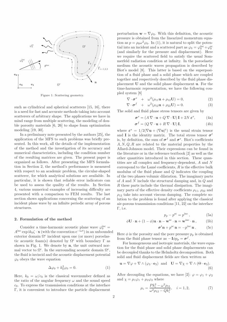
Figure 1: Scattering geometry.

such as cylindrical and spherical scatterers [15, 16], thereis a need for fast and accurate methods taking into accountscatterers of arbitrary shape. The applications we have inmind range from multiple scattering, the modeling of dou-ble porosity materials [6, 26] to shape foam optimizationmodeling [19, 30].

In a preliminary note presented by the authors [25], theapplication of the MFS to such problems was briefly pre-sented. In this work, all the details of the implementationof the method and the investigation of its accuracy andnumerical characteristics, including the condition numberof the resulting matrices are given. The present paper isorganized as follows. After presenting the MFS formula-tion in Section 2, the method’s performance is measuredwith respect to an academic problem, the circular-shapedscatterer, for which analytical solutions are available. Inparticular, it is shown that reliable error indicators canbe used to assess the quality of the results. In Section4, various numerical examples of increasing difficulty arepresented with a comparison to FEM results. The lastsection shows applications concerning the scattering of anincident plane wave by an infinite periodic array of porousstructures.

2. Formulation of the method

Consider a time-harmonic acoustic plane wave ϕinc0 =

Ainc exp ik0ζ · x (with the convention e−iωt) in an unboundedexterior domain Ωe incident upon one (or more) poroelas-tic acoustic foam(s) denoted by Ωi with boundary Γ asshown in Fig. 1. We denote by n, the unit outward nor-mal vector to Ωi. In the surrounding acoustic domain Ωe,the fluid is inviscid and the acoustic displacement potentialϕ0 obeys the wave equation

∆ϕ0 + k20ϕ0 = 0. (1)

Here, k0 = ω/c0 is the classical wavenumber defined asthe ratio of the angular frequency ω and the sound speedc0. To express the transmission conditions at the interfaceΓ, it is convenient to introduce the particle displacement

perturbation w = ∇ϕ0. With this definition, the acousticpressure is obtained from the linearized momentum equa-tion as p = ρ0ω

2ϕ0. In (1), it is natural to split the poten-tial into an incident and a scattered part as ϕ0 = ϕinc

0 +ϕsc0

(and similarly for the pressure and displacement). Herewe require the scattered field to satisfy the usual Som-merfeld radiation condition at infinity. In the poroelasticmedium the acoustic waves propagation is described byBiot’s model [8]. This latter is based on the superposi-tion of a fluid phase and a solid phase which are coupledtogether and respectively described by the fluid phase dis-placement U and the solid phase displacement u. For thetime-harmonic representation, we have the following cou-pled system [8]

∇ · σs + ω2(ρ11u+ ρ12U) = 0, (2)

∇ · σf + ω2(ρ12u+ ρ22U) = 0. (3)

The solid and fluid phase stress tensors are given by

σs = (A∇ · u+Q∇ ·U) I+ 2N ε

s, (4a)

σf = (Q∇ · u+R∇ ·U) I, (4b)

where εs = 1/2(∇u + (∇u)t) is the usual strain tensor

and I is the identity matrix. The total stress tensor σt

is, by definition, the sum of σf and σs. Biot’s coefficients

A,N,Q,R are related to the material properties by theAllard-Johnson model. Their expressions can be found inthe literature or in the reference textbook [2] as well as theother quantities introduced in this section. These quan-tities are all complex and frequency-dependent, A and Ncorrespond to the Lame coefficients, R is the effective bulkmodulus of the fluid phase and Q indicates the couplingof the two phases volumic dilatation. The imaginary partsof A and N include the structural damping and, in Q andR these parts include the thermal dissipation. The imagi-nary parts of the effective density coefficients ρ11, ρ22 andρ12 take into account viscous damping. The complete so-lution to the problem is found after applying the classicalair-porous transmission conditions [11, 22] on the interfaceΓ, i.e.

pp − psc = pinc , (5a)

φU · n+ (1 − φ)u · n−wsc · n = winc · n , (5b)

σtn+ psc n = −pinc n . (5c)

Here φ is the porosity and the pore pressure pp is obtainedfrom the fluid phase tensor as − Iφpp = σ

f .For homogeneous and isotropic materials, the wave equa-

tion for the fluid phase and solid phase displacements canbe decoupled thanks to the Helmholtz decomposition. Bothsolid and fluid displacement fields are then written as

u = ∇ϕ+∇∧ (ϕ3 · e3) and U = ∇χ+∇∧ (Θ · e3).(6)

After decoupling the equations, we have [2]: ϕ = ϕ1 + ϕ2

and χ = µ1ϕ1 + µ2ϕ2 where

µi =Pk2i − ω2ρ11ω2ρ12 −Qk2i

, i = 1, 2, (7)

2

are the wave amplitude ratios between the two phases inthe porous material (here, P = A + 2N). Similarly, thepotential Θ is simply obtained as Θ = µ3ϕ3 with µ3 =ρ12/ρ22. Under this form, each potential ϕi (i = 1, 2, 3)satisfies the Helmholtz equation

∆ϕi + k2i ϕi = 0, (8)

and the associated complex wavenumbers are

k21 =ω2

2(PR−Q2)(Pρ22 +Rρ11 − 2Qρ12 +

√D), (9)

k22 =ω2

2(PR−Q2)(Pρ22 +Rρ11 − 2Qρ12 −

√D), (10)

k23 =ω2

N

(

ρ11ρ22 − ρ212ρ22

)

. (11)

Here, D stands for the discriminant of a quadratic equationand D = (Pρ22 +Rρ11 − 2Qρ12)

2 − 4(PR−Q2)(ρ11ρ22 −ρ212). Physically, there are two compressional waves asso-ciated with ϕ1, ϕ2 and one rotational (shear) wave asso-ciated with ϕ3. They all propagate in the two phases andtheir relative contributions are given by the coefficientsµi. If such a decomposition holds in elastodynamics, thecoexistence of two phases in the poroelastic media adds an-other fluid-borne compressional wave which is not presentis elastic solids.

The MFS implementation starts by choosing an appro-priate set of fundamental solutions for both propagativedomains Ωe and Ωi. In the acoustic domain, a naturalchoice is to choose these solutions using the well-knownfree field Green’s function, i.e. G0(x,y) = i/4H0(k0 |x− y|).So, we seek the scattered field as a distribution of monopoles

psc(x) = ρ0ω2

Q0∑

q0=1

A0q0G0(x,y

0q0), (12)

where the source points y0q0

are chosen to be located on

a curve Γ0 in the interior domain Ωi. The displacementvector is obtained by simply taking the gradient of (12).To simulate the wave field in the foam, a possible choiceis to use fundamental solutions for poroelastic media forwhich an explicit form can be found, for instance, in [9].An easier option is to construct these solutions by simplyexpanding each potential in the form

ϕi(x) =

Qi∑

qi=1

AiqiGi(x,y

iqi), for i = 1, 2, 3, (13)

where Gi(x,y) = i/4H0(ki |x− y|) is the fundamental so-lution of the Helmholtz equation. Here, Qi is the numberof source points yi

qiassociated with the ith potential and

the Aiqi’s are unknown amplitudes. These points are lo-

cated on a fictitious boundary Γi in the exterior domainΩe as shown in Fig. 1. The influence of the location ofthe source points on the quality of the solution will be dis-cussed in the next section. Now, using these expansions in

(6), we find the expression for the different physical quan-tities involved:

φpp(x) =

2∑

i=1

k2i (Q + µiR)

Qi∑

qi=1

AiqiGi(x,y

iqi) (14a)

u(x) =

2∑

i=1

Qi∑

qi=1

Aiqi∇Gi(x,y

iqi) +

Q3∑

q3=1

A3q3∇⊥G3(x,y

3q3)

(14b)

U(x) =2

∑

i=1

Qi∑

qi=1

Aiqiµi∇Gi(x,y

iqi)

+

Q3∑

q3=1

A3q3µ3∇⊥G3(x,y

3q3) (14c)

where ∇⊥ ≡ (∂x2,−∂x1

)tstands for the orthogonal gradi-

ent operator. From these expressions and using (4), we fi-nally obtain the normal total stress tensor σt. The explicitforms for the tensor coefficients are too cumbersome to beinserted in this paper. Note that other type of solutionscould have been considered (Green’s functions and/or theirderivatives or plane waves for instance) and the presentchoice was mainly motivated by simplicity. Furthermore,it has the advantage of allowing us to specify indepen-dently the number of source points Qi for each kind ofwave, which is not the case when using Green’s functions.In this respect, our method is not strictly speaking an MFSsince it does not rely on Biot’s equations fundamental ten-sor.

Now, given a set of Ncol collocation points xl (l =1, . . . , Ncol) on Γ, substituting (14) in the transmissionconditions (5) at each collocation point yields three lin-ear systems of the form

MαA = Fincα , α = a, b, c. (15)

Here, the subscript α refers to the type of condition in-volved (there is one system for each condition (5a), (5b),(5c)). The right hand side vector Finc

α stems from the in-cident wave (pressure and displacement). The unknownvector A contains the amplitudes of all sources. Since theacoustic displacement is expected to behave like |w| ∼k0φ0, it is judicious to rescale the kinematic conditions(5b) by multiplying the associated lines by ρ0c0ω. Thisyields the matrix system

MA = Finc. (16)

In this work, early results showed that it is preferable forreasons of stability to consider more collocation pointsthan the number of unknowns Ndof =

∑3

i=0 Qi. To bemore specific, it was found that taking Ncol = 2Ndof guar-antees that results have converged, i.e. the numerical so-lution becomes insensitive to the number of collocationpoints, as discussed in [3]. All calculations were performedusing this ratio. Note that when dealing with ‘nice’ shaped

3

scatterers (the circular scatterer for instance), the MFShas been observed to perform slightly better with inter-polation schemes (i.e. Ncol = Ndof) than least-squaresschemes (Ncol > Ndof). However, for the sake of robust-ness and generality the second approach was preferred.After multiplying the system (16) by the Hermitian trans-pose M† we finally get the Hermitian square system

M†MA = M†Finc. (17)

A important advantage of performing this operation is thata simple error estimator is available at very low cost. In-deed, going back to the original collocation problem (15),we can define the a posteriori algebraic error estimator foreach of the conditions at the interface (α = a, b, c). Wethus define

Eα = 100

∥

∥MαA− Fincα

∥

∥

2

‖Fincα ‖2

, (18)

where A is solution of (17). The numerical evaluation of(18) is computationally cheap since the matrices Mα havealready been calculated. Of course, taking Ncol = Ndof

will automatically produce errors with zero value (exceptfrom when interpolation matrices are very ill-conditioned).By increasing the number of collocation points, errors willgrow until it stabilises.

As for the choice of positions of the source points, wefollow Alves [3] and take these points along the discretenormal direction, so we put yi

qi= yi

qi+ si ni

qiwhere the

points yiqi

(qi = 1, . . . , Qi and i = 0, . . . , 3) are distributed

on Γ and niqi

is the approximate normal vector defined by

niqi=

(yiqi+1 − yi

qi−1)⊥

maxqi |yiqi+1 − yi

qi−1|. (19)

Here, the symbol ⊥ signifies that we take the orthogo-nal vector pointing outward. The normalization is chosenhere for convenience to ensure that the normal vector am-plitudes never exceed unity and that coefficients si corre-spond to the farthest distance from the interface Γ.

Before we end this section, we should point out that,as far as engineering applications are concerned, the phys-ical variables of primary interest are the pressure and thenormal velocity at the interface. In practical terms, thescattering characteristics of the porous obstacle are con-veniently quantified by the scattering cross section (SCS)defined as the ratio between the scattered power and theincident power flux [23]

Σ =W sc

I inc=

∫

ΓRe (pscvscn ) dΓ

|Ainc|2 ω4ρ0/c0, (20)

where vscn = −iωwsc · n is the normal acoustic velocity forthe scattered field. Similarly, we can define the absorp-tion cross section as the ratio between the total power andthe incident power flux. These quantities combine the re-flection, transmission and the absorption properties of the

porous scatterer. By construction, the SCS is a far fieldestimator and numerical errors at the interface only havea mild impact on its numerical evaluation. This will becommented further when necessary.

3. Validations for the circular-shaped scatterer

We shall validate and assess the efficiency of the methodin the specific case of the scattering of a horizontal acous-tic plane wave by a circular-shaped poroelastic scatterer.In polar co-ordinates, the inner and outer wave fields canbe represented by separable solutions. Each potential isgiven by infinite series which are well behaved allowing usto produce very accurate results without deterioration athigh frequency. The derivation of the exact form for thesesolutions is quite lengthy and this is inserted in Appendix.For a proper assessment of the method’s performance, itis convenient to define the relative error on the boundaryfor each physical quantity (call it X):

E(X) = 100

∥

∥

∥X− X

∥

∥

∥

2∥

∥

∥X

∥

∥

∥

2

, (21)

where X represents either the acoustic pressure, the fluidphase or solid phase normal displacement or the normalstress at the interface and X is the associated vector con-taining the value of X at the collocation points. Here, Xstands for a reference solution vector, either obtained ana-lytically in the present case or computed numerically withanother method when analytical solutions are not avail-able. The aim of this section is to identify the effects ofthe main parameters of the problem, namely the locationsand the number of sources. For this latter, we are stillleft with the problem of finding a quasi-optimal relation-ship between the Qi’s. Through intensive calculations, notpresented here, we found that choosing the same numberfor each wave type was probably the best option offeringthe best trade-off between accuracy, conditioning and sim-plicity. This simplifies the analysis significantly as we cannow put

Q = Qi for i = 0, . . . , 3, (22)

and perform the analysis with a single parameter Q. Sim-ilarly, we take the points yi

qiall equal and put si = s with

s0 = −s. Note that this choice seems to be contrary tothe results given in [27] where it is advocated that thebest option, when using plane waves, is precisely not totake the same number of wave directions for each type ofwaves (that is shear and pressure wave types in the elas-ticity case) and this is particularly relevant when the ratiobetween the wavenumbers is large. The reasons for thisprobably lie in that, plane waves and singular sources be-have differently in terms of their approximation propertiesand it would be interesting to explore this further via nu-merical experiments in the spirit of [4] for instance.

4

Material φ σ (kNm-4s) αinf Λ (µm) Λ′ (µm) ρ1 (kgm-3) N (kPa) ν Ref.

XFM foam 0.98 13.5 1.7 80 160 30 200(1 - 0.05i) 0.35 [11]B wool 0.95 23 1 54.1 162.3 58 8.5(1 - 0.1i) 0 [12]

Table 1: Materials properties. With the resistivity σ, the tortuosity αinf , the viscous and thermal characteristic lengths Λ and Λ′, the poissoncoefficient ν and the effective skeleton density ρ1. The effective skeleton density ρ1 = (1−φ)ρs, where ρs is the density of the material of theframe.

0 20 40 60 80 100 120 140 160−8

−7

−6

−5

−4

−3

−2

−1

0

1

2

logE

Q

(a)

0 20 40 60 80 100 120 140 1602

4

6

8

10

12

14

16

18

20

Q

logcond2

(b)

Figure 2: Effects of the sources location on the error and the condi-tioning ( s = 0.1a, s = 0.2a, s = 0.3a). (a): error onthe solid phase normal displacement for the XFM foam at 1500Hz;line with markers ‘·’ refers to E(un) error and the simple line to thea posteriori error Eb. (b): conditioning (2-norm) of M†

M.

As an exemple we chose a polymer foam (XFM) com-monly used in the transport industry. The material prop-erties are reported in Table 1. To give an idea of thecomplex wavenumbers for the wave potentials in the ma-terial, we find that k1 ≈ 17.6 + 1.21i, k2 ≈ 21.4 + 14.1iand k3 ≈ 38.9 + 2.1i (these values correspond to the fre-quency 500 Hz). The corresponding acoustic wavenumberis k0 ≈ 9.2. On Fig. 2 (a) we show the influence of thesource locations as well as the number of sources (i.e. Q)on the normal solid displacement error un = u · n, i.e.E(un) and the a posteriori error Eb. The evolution of theconditioning (in the 2-norm) of the associated system isalso shown (Fig. 2 (b)). Before we comment on these re-sults, we should point out that we chose to measure thenormal displacement error rather than the pressure errorfor the simple reason that it was observed, that a smallerror on the displacement normally guarantees a smallererror on the pressure. The convergence curves togetherwith the conditioning curves typically illustrate the MFSparadox which many authors have already observed anddiscussed: despite the ill-conditioning of the MFS systems,the method produces accurate results. In the present sit-uation, it is concluded that the further away from theboundary the source points are (i.e. the larger s), thebetter the results as long as the conditioning of the sys-tem does not exceed a certain value above which resultsare likely to be corrupted by round off errors. This value,say cond2 ≈ 1016, is in line with standard double preci-sion arithmetic. Note that, in our algorithm, matrices areinverted using the pinv function from MATLAB so thatfor very ill-conditioned matrices (cond2 > 1016) the SVDsolver is automatically used with some thresholding in or-der to dampen the effects of the round-off errors. In thisrespect, we believe that better results could perhaps beobtained by properly filtering the small singular values.Another approach would be to apply Tikhonov regulariza-tion in order to speed up the computation. In fact, themost striking feature of these convergence curves is the al-most perfect agreement between the true error E(un) andits algebraic counterpart, the a posteriori error Eb andthrough many numerical experiments, we always observedvery good correlations. The mathematical reasons for thisgoes beyond the scope of this paper but we believe thatin most cases the algebraic a posteriori errors Eα shouldserve as reliable error indicators especially when referencesolutions are not available.

5

4. Numerical examples

a

Figure 3: Square-shaped scatterer. Here symbols +, ×, indicatethe location of the source points in Ωe and ♦ those in Ωi. Thecollocation points on Γ are identified by the markers ‘·’.

This section comprises three examples of increasing dif-ficulty illustrating the efficiency of the MFS. The firstshows the MFS performance for foams presenting geo-metrical singularities such as corners. In the second ex-ample, we tackle circular shaped corrugated foams. Thelast example concerns scatterers of arbitrary shapes. Be-cause there are no analytical solutions to these problems,all reference solutions are computed using Finite Elementmodels. These computations are carried using Lagrangequadratic finite elements in both fluid and poroelastic do-mains. The (u, pp) formulation of Biot’s equations [5, 11] isused and the non reflecting boundary conditions are imple-mented using Bermudez’s perfectly matched layer (PML)formulation [7]. As for the accuracy of these FE refer-ence solutions, numerical tests carried out on the circularshaped scattering problem shows that these results are re-liable up to around 1 percent of error on the solid phasenormal displacement which is acceptable if engineering ac-curacy is sought.

4.1. Square scatterer

The first example concerns that of a square-shapedporoelastic scatterer of side length a = 0.2 m. The in-cident plane wave is horizontal, travelling in the ζ = (1, 0)direction and the frequency is 1500 Hz. In this scenario,the boundary curve is not regular and source points aroundthe square are placed along the normal to the boundaryavoiding the corners, see Fig. 3. In this respect, we foundthat putting more sources in the vicinity of the cornersdid not show any improvement. Comparisons between theMFS and the FE results are conveniently shown in Fig. 4for the pressure (Fig. 4a) and the normal displacement(Fig. 4b). Here, the abscissae θ refers the usual polar co-ordinate of the collocation points on the boundary (the

square is centered at the origin). One can note the as-sociated global errors are in good agreements with the a

posteriori error estimator as shown in Table 2.As expected, the discrepancies reach a maximum near

the corners and this is particularly noticeable for the dis-placement curve. The pressure remains more stable evennear the corners and is free of spurious oscillations. For-tunately these spurious oscillations, present on the nor-mal displacement curve have a low radiation efficiency andtheir effect on the SCS is negligible.

We should point out that, the displacement and pres-sure magnitudes do not correspond to any realistic case aswe took Ainc = 1 in our calculations.

−1.5

−1

−0.5

0.5

1x 10

8

θ (rad)

Rep(P

a)

−π −π2

0

0 π2 π

(a)

−2.5

−2

−1.5

−1

−0.5

0.5

1

1.5

θ (rad)

Reun(m

)

−π −π2

0

0 π2 π

(b)

Figure 4: (a): Real part of the pressure field on Γ at 1500 Hz for thesquare-shaped scatterer; solid line: FEM solution and dots refers tothe MFS solution. (b): Real part of solid phase normal displacement.

4.2. Scattering by a corrugated cylinder

Here, we consider the scattering of a horizontal planewave by a circular shaped corrugated foam with boundary

6

Table 2: Relative errors on a square scatterer (a=0.2 m, s=0.2a) at500 Hz and 1500 Hz for XFM foam with Q=60 and 2 × 4Q = 480collocation points.

500 Hz 1500 Hz

Fields Eα (%) E (%) Eα (%) E (%)

p (α =a) 5.56 0.75 3.95 1.03u · n (α =b) 4.42 1.88 4.95 4.31

given parametrically by

x(t) = 0.1

(

cos tsin t

)

+ 0.005

(

cos 8tsin 8t

)

, t ∈ [0, 2π[. (23)

The shape of the boundary as well as the location of thecollocation points and the source points are displayed inFig. 5. The perfectly circular shape of radius a = 0.1 mis also illustrated. For this specific example, a multifre-quency analysis is performed in the range [0,5000 Hz]. InFig. 6 we show the evolution of the SCS for different mate-rials: the XFM foam and the B wool whose properties arereported in Table 1. The perfectly circular shape is alsoconsidered for the sake of illustration. The results are com-pared with the perfectly reflecting wall case (rigid wall).These are computed using the MFS with acoustic sourcesonly and by applying the normal displacement conditionat the interface: w · n = 0.

In the mid-frequency range, the presence of peaks forthe XFM foam can be observed. An analysis of the poroe-lastic wave field in the absorbing material reveals thatthese are due to some resonance effects of the elastic foam’sskeleton. For the wool, these peaks are highly attenuatedand the use of an equivalent fluid model [12] would havebeen sufficient for the analysis. The effects of the cor-rugations on the SCS are noticeable above 3000 Hz forthe rigid case. This frequency corresponds to an acous-tic wavelength which is comparable to the length of theobstacle. For porous scatterers, the effects of the corruga-tions are dampened due to the absorbing properties of thematerials, especially in the high-frequency range.

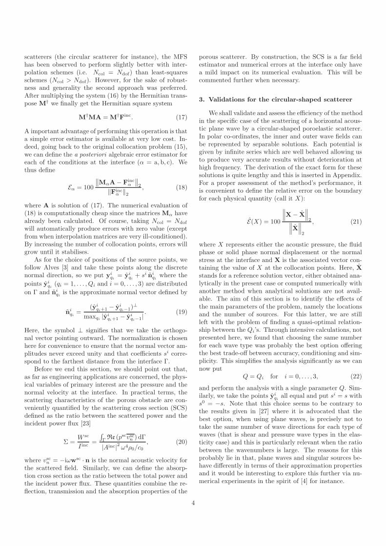
All the results have been computed with an accuracythat does not exceed 1.2% error. A closer analysis, how-ever, is instructive as it shows behaviors which are inherentto the method. In Fig. 7, the associated a posteriori errorsEb are plotted in logarithmic scale. For the rigid circularcylinder case, clearly identifiable peaks can be observed atthe frequencies: 1626, 2592 and 3733 Hz. These peaks cor-respond to a loss of accuracy due to some non-uniquenessproblems of the MFS formulation. This point is discussedin length in [32] and in [10] for the circular cylinder case.It emerges that these ‘critical’ frequencies are in fact theeigenvalues of an interior problem corresponding to theinternal surface on which are located the source points.Because the source points are placed on a perfectly circu-lar ring, it was easy to check that the frequencies corre-spond to the interior Dirichlet problem [10]. In general,

a

Figure 5: Corrugated cylinder shape. Here +, ×, are the sourcepoints in Ωe and ♦ those in Ωi. The collocation points on Γ are givenby markers ‘·’.

0 1000 2000 3000 4000 50000

0.2

0.4

Σ(m

)

f (Hz)

Figure 6: Scattering cross section for the straight (black) and corru-gated cylinder (gray). XFM foam, B wool, rigid wall.Computed using Q = 60.

these irregular frequencies are hard (if not impossible) topredict though their effects are somewhat noticeable evenwith porous scatterers (except with the B wool where it isharder to conclude).

In this work, the MFS algorithm was implemented us-ing MATLAB and, for the specific examples illustratedhere, around 0.73 second (CPU time) is needed per fre-quency (Intel Core 2 Duo T7100 @ 1.80 GHz, 2 GB RAM).To the authors’ knowledge these performances cannot bemet with the FEM. Using a compiled language and avoid-ing some redundant evaluations of Hankel functions, it isanticipated that the computational time could be reducedfurther by a factor of 10. For the sake of illustration, thetotal pressure field is shown in Fig. 8. This corresponds toa high frequency calculation (15000 Hz). Around 1.6 sec-onds are required to compute the solution with less than

7

0 1000 2000 3000 4000 5000−4.5

−4

−3.5

−3

−2.5

−2

−1.5

−1

−0.5

0

logE b

f (Hz)

Figure 7: a posteriori error estimator for the straight (black) andcorrugated (gray) cylinder. XFM foam, B wool, rigidwall. Computed using Q = 60.

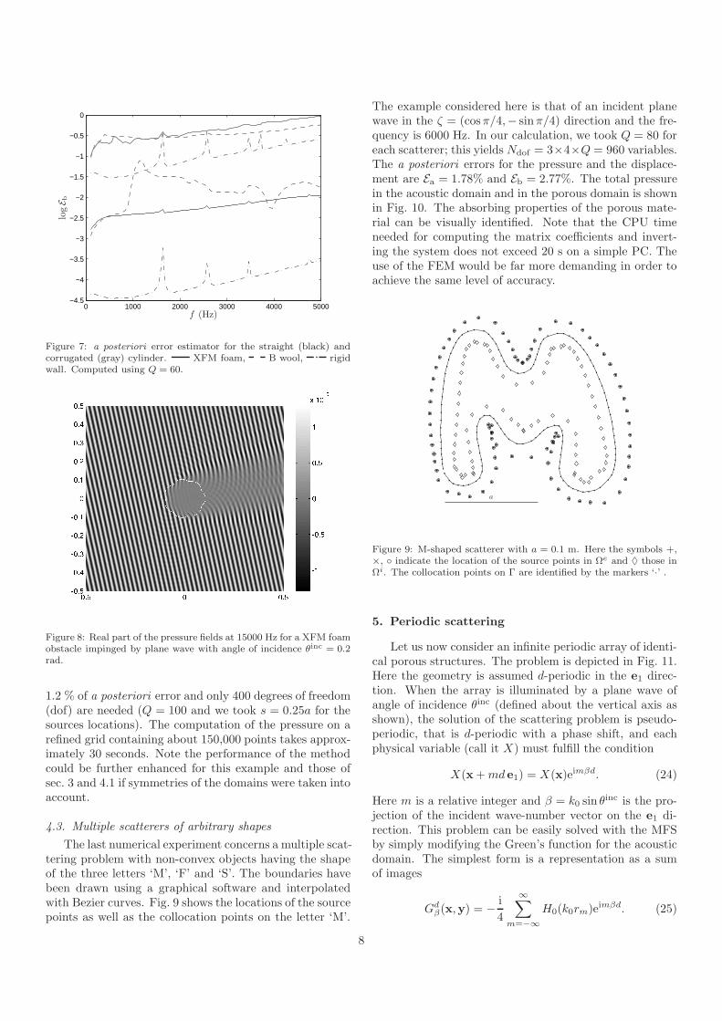
Figure 8: Real part of the pressure fields at 15000 Hz for a XFM foamobstacle impinged by plane wave with angle of incidence θinc = 0.2rad.

1.2 % of a posteriori error and only 400 degrees of freedom(dof) are needed (Q = 100 and we took s = 0.25a for thesources locations). The computation of the pressure on arefined grid containing about 150,000 points takes approx-imately 30 seconds. Note the performance of the methodcould be further enhanced for this example and those ofsec. 3 and 4.1 if symmetries of the domains were taken intoaccount.

4.3. Multiple scatterers of arbitrary shapes

The last numerical experiment concerns a multiple scat-tering problem with non-convex objects having the shapeof the three letters ‘M’, ‘F’ and ‘S’. The boundaries havebeen drawn using a graphical software and interpolatedwith Bezier curves. Fig. 9 shows the locations of the sourcepoints as well as the collocation points on the letter ‘M’.

The example considered here is that of an incident planewave in the ζ = (cosπ/4,− sinπ/4) direction and the fre-quency is 6000 Hz. In our calculation, we took Q = 80 foreach scatterer; this yields Ndof = 3×4×Q = 960 variables.The a posteriori errors for the pressure and the displace-ment are Ea = 1.78% and Eb = 2.77%. The total pressurein the acoustic domain and in the porous domain is shownin Fig. 10. The absorbing properties of the porous mate-rial can be visually identified. Note that the CPU timeneeded for computing the matrix coefficients and invert-ing the system does not exceed 20 s on a simple PC. Theuse of the FEM would be far more demanding in order toachieve the same level of accuracy.

a

Figure 9: M-shaped scatterer with a = 0.1 m. Here the symbols +,×, indicate the location of the source points in Ωe and ♦ those inΩi. The collocation points on Γ are identified by the markers ‘·’ .

5. Periodic scattering

Let us now consider an infinite periodic array of identi-cal porous structures. The problem is depicted in Fig. 11.Here the geometry is assumed d-periodic in the e1 direc-tion. When the array is illuminated by a plane wave ofangle of incidence θinc (defined about the vertical axis asshown), the solution of the scattering problem is pseudo-periodic, that is d-periodic with a phase shift, and eachphysical variable (call it X) must fulfill the condition

X(x+md e1) = X(x)eimβd. (24)

Here m is a relative integer and β = k0 sin θinc is the pro-

jection of the incident wave-number vector on the e1 di-rection. This problem can be easily solved with the MFSby simply modifying the Green’s function for the acousticdomain. The simplest form is a representation as a sumof images

Gdβ(x,y) = − i

4

∞∑

m=−∞

H0(k0rm)eimβd. (25)

8

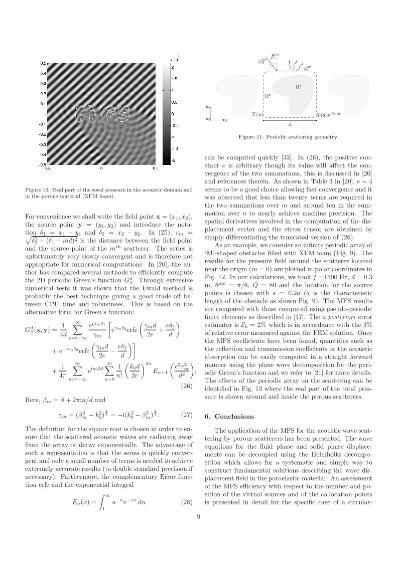
Figure 10: Real part of the total pressure in the acoustic domain andin the porous material (XFM foam).

For convenience we shall write the field point x = (x1, x2),the source point y = (y1, y2) and introduce the nota-tion δ1 = x1 − y1 and δ2 = x2 − y2. In (25), rm =√

δ22 + (δ1 −md)2 is the distance between the field pointand the source point of the mth scatterer. The series isunfortunately very slowly convergent and is therefore notappropriate for numerical computations. In [20], the au-thor has compared several methods to efficiently computethe 2D periodic Green’s function Gd

β . Through extensivenumerical tests it was shown that the Ewald method isprobably the best technique giving a good trade-off be-tween CPU time and robustness. This is based on thealternative form for Green’s function:

Gdβ(x,y) =

1

4d

∞∑

m=−∞

eiβmδ1

γm

[

eγmδ2erfc

(

γmd

2e+

eδ2d

)

+ e−γmδ2erfc

(

γmd

2e− eδ2

d

)]

+1

4π

∞∑

m=−∞

eimβd

∞∑

n=0

1

n!

(

k0d

2e

)2n

En+1

(

e2r2md2

)

,

(26)

Here, βm = β + 2πm/d and

γm = (β2m − k20)

1

2 = −i(k20 − β2m)

1

2 . (27)

The definition for the square root is chosen in order to en-sure that the scattered acoustic waves are radiating awayfrom the array or decay exponentially. The advantage ofsuch a representation is that the series is quickly conver-gent and only a small number of terms is needed to achieveextremely accurate results (to double standard precision ifnecessary). Furthermore, the complementary Error func-tion erfc and the exponential integral

En(x) =

∫ ∞

1

u−ne−xu du (28)

θinc

Ωe

Ωi

e1

e2

e3X(x)eiβmdX(x)

ϕinc0

ϕsc0

d

Figure 11: Periodic scattering geometry.

can be computed quickly [33]. In (26), the positive con-stant e is arbitrary though its value will affect the con-vergence of the two summations, this is discussed in [20]and references therein. As shown in Table 3 in [20], e = 4seems to be a good choice allowing fast convergence and itwas observed that less than twenty terms are required inthe two summations over m and around ten in the sum-mation over n to nearly achieve machine precision. Thespatial derivatives involved in the computation of the dis-placement vector and the stress tensor are obtained bysimply differentiating the truncated version of (26).

As an example, we consider an infinite periodic array of‘M’-shaped obstacles filled with XFM foam (Fig. 9). Theresults for the pressure field around the scatterer locatednear the origin (m = 0) are plotted in polar coordinates inFig. 12. In our calculations, we took f =1500 Hz, d = 0.3m, θinc = π/6, Q = 80 and the location for the sourcepoints is chosen with s = 0.2a (a is the characteristiclength of the obstacle as shown Fig. 9). The MFS resultsare compared with those computed using pseudo-periodicfinite elements as described in [17]. The a posteriori errorestimator is Eb = 2% which is in accordance with the 3%of relative error measured against the FEM solution. Oncethe MFS coefficients have been found, quantities such asthe reflection and transmission coefficients or the acousticabsorption can be easily computed in a straight forwardmanner using the plane wave decomposition for the peri-odic Green’s function and we refer to [21] for more details.The effects of the periodic array on the scattering can beidentified in Fig. 13 where the real part of the total pres-sure is shown around and inside the porous scatterers.

6. Conclusions

The application of the MFS for the acoustic wave scat-tering by porous scatterers has been presented. The waveequations for the fluid phase and solid phase displace-ments can be decoupled using the Helmholtz decompo-sition which allows for a systematic and simple way toconstruct fundamental solutions describing the wave dis-placement field in the poroelastic material. An assessmentof the MFS efficiency with respect to the number and po-sition of the virtual sources and of the collocation pointsis presented in detail for the specific case of a circular-

9

−1.5

−1

−0.5

0.5

1

1.5x 10

8

θ (rad)

Rep(P

a)

−π −π2

0

0 π2 π

Figure 12: Real part of the pressure field around a M-shaped scat-terer (m = 0) at 1500 Hz. The marker ‘·’ refers to the FEM solutionand ‘+’ to the MFS solution.

Figure 13: Real part of the MFS pressure field at 1500 Hz for aperiodic ‘M’-shaped porous scatterer.

shaped scatterer. In particular, it is shown that reliableerror indicators can be used to assess the quality of theresults. Through many illustrative examples of increas-ing difficulty, comparisons with results computed using amixed pressure-displacement finite element formulation il-lustrate the considerable advantages of the MFS both interms of computational resources and mesh preparation.Finally, the extension of the method to dealing with theacoustic wave scattering by an infinite array of periodicporous scatterers is discussed and presented. It is believedthat the method show promise in solving a wide range ofnoise control problems ranging from multiple scattering toshape foam optimization. The development of the MFSfor 3D problems is also of particular interest to us andthis could be the subject of futur work.

Acknowledgement

The authors wish to thank the Projet Pluri-FormationsPilcam2 [28] at the Universite de Technologie de Compiegnefor providing the high performance computing resourcesthat have contributed to the research results reported withinthis paper as well as the reviewers for their helpful com-ments.

Appendix A. Scattering of a horizontal acoustic

plane wave by a circular-shaped poroe-

lastic scatterer.

Take an incident plane wave along the e1 direction withamplitude Ainc. Following [1, 23], the outer wave fieldin the acoustic domain can be represented by separablesolutions in polar coordinates (r, θ) as

ϕinc0 = Ainceik0x1 = Ainceik0r cos θ (A.1)

= Ainc

[

J0(k0r) + 2

∞∑

m=1

imJm(k0r) cosmθ

]

, (A.2)

and, similarly for the total field:

ϕ0 = ϕinc0 +

∞∑

m=0

A0,mHm(k0r) cosmθ. (A.3)

For the wave field in the poroelastic medium we can fol-low a recent paper [24] and expand each potential as theFourier series:

ϕi =

∞∑

m=0

Ai,mJm(kir) cosmθ, with i = 1, 2, (A.4a)

ϕ3 =

∞∑

m=0

A3,mJm(k3r) sinmθ. (A.4b)

Now, applying the boundary conditions (5) at the air-porous interface r = a yields a linear system of the form

MAm = F (A.5)

where all the quantities involved depend on the azimuthalmode number m = 0, 1, 2.... The resolution of this 4 × 4matrix system gives the coefficients Ai,m (i = 0, . . . , 3)and the analytical solution can thus be computed. Forcompleteness, the analytical expressions for the coefficientsare explicitly written:

M1,1 =ρ0ω2Hm(k0a) (A.6a)

M1,2 =− k21Jm(k1a)(

Q+ µ1R)

φ(A.6b)

M1,3 =− k22Jm(k2a)(

Q+ µ2R)

φ(A.6c)

M1,4 =0 (A.6d)

10

M2,1 =−k0Hm+1(k0a)a+mHm(k0a)

a(A.6e)

M2,2 =− φ1

(

− k1Jm+1(k1a)a+mJm(k1a))

a(A.6f)

M2,3 =− φ2

(

− k2Jm+1(k2a)a+mJm(k2a))

a(A.6g)

M2,4 =− Jm(k3a)mφ3

a(A.6h)

M3,1 =− ρ0ω2Hm(k0a) (A.6i)

M3,2 =−2Nk1Jm+1(k1a)a+ Jm(k1a)C1

a2(A.6j)

M3,3 =−2Nk2Jm+1(k2a)a+ Jm(k2a)C2

a2(A.6k)

M3,4 =−2mN

a2(

− k3Jm+1(k3a)a+ Jm(k3a)(m− 1))

(A.6l)

M4,1 =0 (A.6m)

M4,2 =2mN

a2(

− k1Jm+1(k1a)a+ Jm(k1a)(m− 1))

(A.6n)

M4,3 =2mN

a2(

− k2Jm+1(k2a)a+ Jm(k2a)(m− 1))

(A.6o)

M4,4 =− N

a2(

− 2k3Jm+1(k3a)a

+ Jm(k3a)(−2m2 + 2m+ k23a2))

, (A.6p)

with the constants

Ci = k2i(

(Q+R)µi + P +Q)

a2 − 2mN(m− 1), (A.7)

and φi =(

φµi+1−φ)

. The right hand side vector containsthe contributions from the incident plane wave:

F1 =− 2ρ0ω2AincimJm(k0a) (A.8a)

F2 =2

aAincim

(

k0Jm+1(k0a)a−mJm(k0a))

(A.8b)

F3 =2ρ0ω2AincimJm(k0a) (A.8c)

F4 =0. (A.8d)

and these coefficients have to be divided by 2 for the specialcase m = 0. The conditioning of the system can be im-proved by multiplying the line of M corresponding to thenormal displacement condition by the factor ρ0c0ω (andsimilarly for the corresponding line of F). In practice, thesummation of the series is carried out until the relative dif-ference between two consecutive steps is lower than 10−10

percent.

References

[1] A. Abramowitz, I. Stegum, Handbook of Mathematical func-tions, New York, Dover Publ, 1965.

[2] J.F. Allard, Propagation of sound in porous media: modelingsound absorbing materials, Chapman & Hall, 1993.

[3] C.J.S. Alves, On the choice of source points in the method offundamental solutions, Engng. Anal. Bound. Elem 33 (2009)1348–1361.

[4] C.J.S. Alves, S.S. Valtchev, Numerical comparison of two mesh-free methods for acoustic wave scattering, Engng. Anal. Bound.Elem 29 (2005) 371–382.

[5] N. Atalla, M.A. Hamdi, R. Panneton, Enhanced weak inte-gral formulation for the mixed (u, p) poroelastic equations, J.Acoust. Soc. Am. 109 (2001) 3065–3068.

[6] N. Atalla, R. Panneton, F.C. Sgard, X. Olny, Acoustic absorp-tion of macro-perforated porous materials, J. Sound Vib. 243(2001) 659–678.

[7] A. Bermudez, L. Hervella-Nieto, A. Prieto, R. Rodriguez, Anoptimal perfectly matched layer with unbounded absorbingfunction for time-harmonic acoustic scattering problems, J.Comput. Phy. 223 (2007) 469–488.

[8] M.A. Biot, Theory of propagation of elastic waves in a fluid-saturated porous solid. I. low-frequency range., J. Acoust. Soc.Am. 28 (1956) 168–191.

[9] G. Bonnet, Basic singular solutions for a poroelastic medium inthe dynamic range, J. Acoust. Soc. Am. 82 (1987) 1758–1762.

[10] I.L. Chen, Using the method of fundamental solutions in con-junction with the degenerate kernel in cylindrical acoustic prob-lems, J. Chin. Inst. Engin. 29 (2006) 445–457.

[11] P. Debergue, R. Panneton, N. Atalla, Boundary conditions forthe weak formulation of the mixed (u, p) poroelasticity problem,J. Acoust. Soc. Am. 106 (1999) 2393–2390.

[12] O. Doutres, N. Dauchez, J.M. Genevaux, O. Dazel, Validity ofthe limp model for porous materials: a criterion based on theBiot theory, J. Acoust. Soc. Am. 122 (2007) 2038–2048.

[13] G. Fairweather, A. Karageorghis, The method of fundamentalsolutions for elliptic boundary value problems, Adv. Comput.Math. 9 (1998) 69–95.

[14] G. Fairweather, A. Karageorghis, P.A. Martin, The method offundamental solutions for scattering and radiation problems,Engng. Anal. Bound. Elem. 27 (2003) 759–769.

[15] S.M. Hasheminejad, S.A. Badsar, Acoustic scattering by a pairof poroelastic spheres, J. Mech. Appl.Math. 46 (2004) 95–113.

[16] S.M. Hasheminejad, R. Sanaei, Acoustic scattering by an ellipticcylindrical absorber, Acta Acustica united with Afcustica 93(2007) 789–803.

[17] A.C. Hennion, R. Bossut, J.N. Decarpigny, C. Audoly, Analysisof the scattering of a plane acoustic wave by a periodic elasticstructure using the finite element method : application to com-pliant tube gratings, J. Acoust. Soc. Am. 87 (1990) 1861–1870.

[18] N.E. Horlin, M. Nordstron, P. Goransson, A 3-D hierarchical feformulation of Biot’s equations for elasto-acoustic modeling ofporous media, J. Sound Vib. 245 (2001) 633–652.

[19] J.S. Lee, Y.Y. Kim, J.S. Kim, Y.J. Kang, Two-dimensionalporoelastic acoustical foam shape design for absorption co-efficient maximization by topology optimization method, J.Acoust. Soc. Am. 123 (2008) 2094–2106.

[20] C.M. Linton, The Green’s function for the two dimensionalHelmholtz equation in periodic domains, J. Engin. Math. 33(1998) 377–402.

[21] C.M. Linton, I. Thompson, Resonant effects in scattering byperiodic arrays, Wave motion 44 (2007) 167–175.

[22] O.L. Lovera, Boundary conditions for a fluid-saturated poroussolid, Geophysics 52 (1987) 174–178.

[23] P.M. Morse, K.U. Ingard, Theoretical acoustics, Princeton Uni-versity Press, 1986.

[24] B. Nennig, E. Perrey-Debain, M. Ben Tahar, A mode matchingmethod for modelling dissipative silencers lined with poroelasticmaterials and containing mean flow, J. Acoust. Soc. Am. 128(2010) 3308–3320.

[25] B. Nennig, E. Perrey-Debain, J.D. Chazot, On the efficiencyof the method of fundamental solutions for acoustic scatteringby a poroelastic material, in: The 32nd International Confer-ence on Boundary Elements and other Mesh Reduction Methods

11

(BEM/MRM), New Forest, UK, pp. 181–193.[26] X. Olny, C. Boutin, Acoustic wave propagation in double poros-

ity media, J. Acoust. Soc. Am. 114 (2005) 73–89.[27] E. Perrey-Debain, Plane wave decomposition in the unit disc:

Convergence estimates and computational aspects, J. Comput.Appl. Math. 193 (2006) 140–156.

[28] Pilcam, http://pilcam2.wikispaces.com, Last visit october2010.

[29] S. Rigobert, N. Atalla, F. Sgard, Investigation of the conver-gence of the mixed displacement-pressure formulation for three-dimensional poroelastic materials using hierarchical elements, J.Acoust. Soc. Am. 114 (2003) 2607–2617.

[30] F.C. Sgard, X. Olny, N. Atalla, F. Castel, On the use of per-forations to improve the sound absorption of porous materials,Appl. Acoust. 66 (2005) 625–651.

[31] O. Tanneau, P. Lamary, Y. Chevalier, A boundary elementmethod for porous media, J. Acoust. Soc. Am. 20 (2006) 1239–1251.

[32] D.T. Wilton, I.C. Mathews, R.A. Jeans, A clarification ofnonexistence problems with the superposition method, J.Acoust. Soc. Am. 94 (1993) 1676–1680.

[33] S. Zhang, J. Jin, Computation of Special Functions, Wiley,1996.

12