Embed Size (px)
Citation preview
Why people move?The migration choice
Alessandra Venturini
The Economics of Migration, 2016

The economic analyses of
migration focus on three main subjects
• The migration choice
• The effect in the destination country
-on the GNP and innovation
-in the labour market
-on the welfare
-integration (wage assimilation)
• The effect in the sending countries
-economic and social remittances,
-brain drain

MethodologyThe research in economics is conditioned upon the dataset available, we use the economic theory and the statistical knowledge to overcome data limitation

The migration choiceWhy do people move?Who does move?How many people do move?
• 95% of the research on labour migrants
• Now some research on refugees (Hatton Tim 2015; Dustmann et al 2016)
• Very little of family reunification


Figure 3 Breakdown of the stock of migrants for each continent of origin (100%) across continents of destination (colours) in 2017 and 1960. Source: own elaboration based on UNDESA and WB.


Figure 7 Distribution of first residence permits for
family reasons by EU MS of destination

Figure 8 Distribution of first residence permits for work reasons by EU MS of destination (left) and by country of origin (right). Source: own elaboration based on EUROSTAT


Alessandra VenturiniEconomics of Migration 2016


Alessandra Venturini
Migration in Europe 2018

Alessandra Venturini
Economics of immigration 2016
Source: World Bank

Alessandra Venturini
Migration in Europe 2018

Why people move?
Lesson 3
Alessandra VenturiniMigration in Europe 2018

Many theories and many approaches• Economic, Sociologic
• Micro, Macro
Alessandra VenturiniMigration in Europe 2018
There is no single theory widely accepted by social scientists to account for emergence and perpetuation of international migration• Fragmented set of theories developed in isolation from one another and usually segmented by disciplinary boundaries e.g. economics
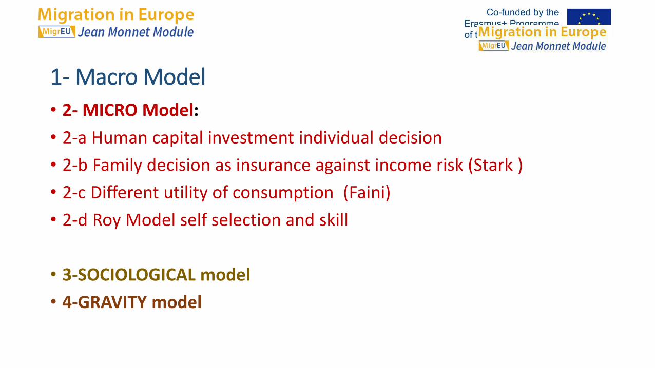
1- Macro Model
• 2- MICRO Model:
• 2-a Human capital investment individual decision
• 2-b Family decision as insurance against income risk (Stark )
• 2-c Different utility of consumption (Faini)
• 2-d Roy Model self selection and skill
• 3-SOCIOLOGICAL model
• 4-GRAVITY model

• Migration theory 1885 British Geographer Ravenstein
• Origin destination migration is function of spatial disequilibria:
• Harris Todaro 1970 economic disequilibria• Lee 1966 demographic disequilibria• PUSH-PULL• Demographic reasons and poverty are not sufficient
conditions• Macro and individual decisions

Macro model 1. HIcks
•Hicks (1932: 76): „differences in net economic advantages,
•Chiefly differences in wages, are the main causes of migration”
Alessandra VenturiniMigration in Europe 2018

Assumptions:
•People are rational and tend to maximize their utility
•People are mobile
•-migration occur without costs
•-there is no risk or uncertainty
Alessandra VenturiniMigration in Europe 2018

Alessandra VenturiniMigration in Europe 2018

2 Micro2.a Individual model Investment in migration (Todaro)• Assumptions:
• Individuals behave in a rational way, they gather all information and
are capable to compare different locations
• Individuals have costless access to perfect information
• Individuals maximize their utility
• Migration has a temporal dimension – preferences regarding time and risk are important, individuals exhibit a more or less preference for the present
• Migration decision is taken individually, social context is neglected.
Alessandra VenturiniMigration in Europe 2018

• Labour mobility according to the human capital theory
• Migration as an investment decision met with an intention to find maximal pay
• for a given level of skills investment which improves the productivity of
human capital
• Idea: workers calculate the value of the employment opportunities available in each of the alternative labour markets, net out the costs of making the move
• and choose option which maximizes the net present value of lifetime earnings
• Migration decision is guided by the comparison of the present value of lifetime
• earnings in the alternative employment opportunities net gain positive
• Problems: risk and uncertainty, costs (pecuniary and non-pecuniary)
Alessandra VenturiniMigration in Europe 2018

• Basic assumption human capital model: • 1 Migration −→ higher wage • 2 Individuals’ choice is based on financial
considerations
• Investment decision:• Costs: direct expenses & forgone earnings• Benefits: higher wage (and employment rate)

Migration – Theory Graphical representation of migration choice

Moving decision – theory
• PVo = wo + wo/(1+r)t ≈ wo+ wo/r
• PVs+1 =−Cs + ws+1 /(1+r)t ≈-Cs+ws+1/r
• Migrate until PVo = PVs+1: (ws+1−wo)/r = wo + Cs
• which means approximately: ∆ws/wo = r
t=1
T
å
t=1
T
å

year 2000 2001 2002
time t t+1 t+2
capital 100
interest rate r 0.10 110 121
interest rate r 0.20 120 144

Alessandra VenturiniMigration in Europe 2018
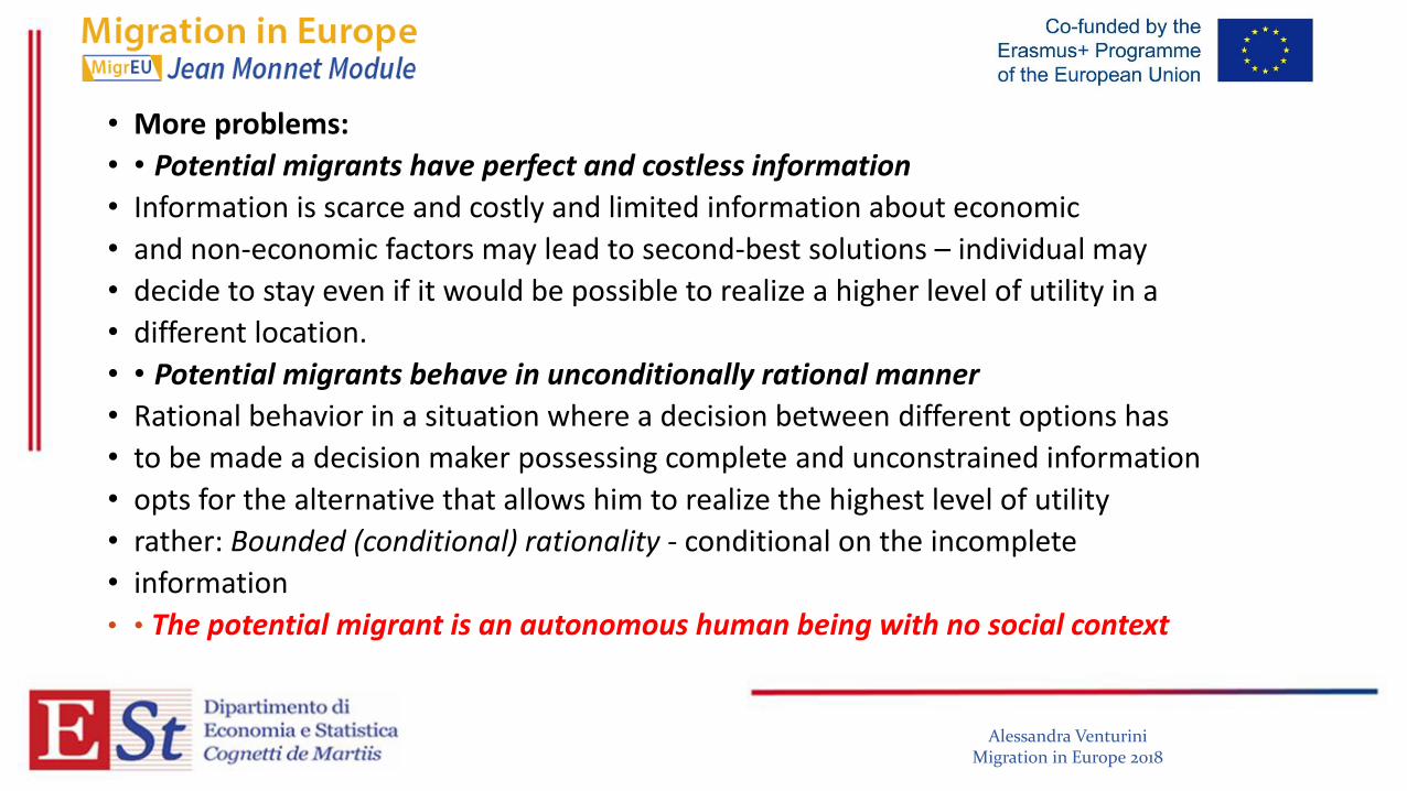
• More problems:
• • Potential migrants have perfect and costless information
• Information is scarce and costly and limited information about economic
• and non-economic factors may lead to second-best solutions – individual may
• decide to stay even if it would be possible to realize a higher level of utility in a
• different location.
• • Potential migrants behave in unconditionally rational manner
• Rational behavior in a situation where a decision between different options has
• to be made a decision maker possessing complete and unconstrained information
• opts for the alternative that allows him to realize the highest level of utility
• rather: Bounded (conditional) rationality - conditional on the incomplete
• information
• • The potential migrant is an autonomous human being with no social context
Alessandra VenturiniMigration in Europe 2018


2.B Family decision as insurance against income risk (Stark )
• Assumptions:
• Labour is a specific factor of production
• Individuals are acting in a social context focus on the family or the household
• Migration is to be perceived as a complex social phenomenon: „Migration can
• be looked upon as a process of innovation, adoption and diffusion” (Stark and Bloom 1985: 176)
• Migration does not have to be permanent, in contemporary world temporary
• mobility is very common.
• Side note: Role of family / houshehold in migration social structures, cognitive structures, gender roles etc. (Mincer, Boyd, Harbison etc.)
Alessandra VenturiniMigration in Europe 2018

Alessandra VenturiniMigration in Europe 2018
Key idea:migration decisions are not made by isolated individuals but by larger units of related people (families, households, communities)people can act collectively not only to maximize expected income but alsoto minimize risk and to loosen constraints associated with various kinds of market failureshouseholds are able to control risks to their economic well-being by diversifying the allocation of resources (family labour) to different labour markets.• Critical risks and market failures: agriculture, labour market, pension system, financial market and credit market

• Migration and risk diversification – an example:
• A village household – 2 adults with following income patterns:
• „Good year” – 100 x 2 = 200
• „Bad year” – 50 x 2 = 100
• What happened if the amount of money necessary to survive equals 150?
• Migration to the town if the income in the town is perfectly negatively
• correlated with village income there is a chance to minimize risk
• completely…
Alessandra VenturiniMigration in Europe 2018

Model 2.C Utility of Consumtion (Faini)


Alessandra VenturiniEconomics of Migration 2016

Empirical version
• Testing the migration choice is very complex
• Which data could we use?
• Individual data with retrospective question
• Aggregate data in the country of destination

Greece Spain Portugal Turkey
Constant -189 (4.17) -160 (1.44) -159 (3.87) -234 (2.6)
LY 45.2 (4.33) 36.7 (1.82) 37.9 (3.77) 57.9 (2.5)
LYSQ -2.7 (4.40) -2.1 (1.77) -2.3 (3.69) -3.6 (2.4)
LDIF 3.4 (1.68) 4.36 (2.72) 3.12 (3.23) .39 (.32)
Ui1 .03 (1.03) -.01 (.56) .42 (3.73) .01 (.33)
Un -.11 (2.30) -.08 (1.07) -.09 (1.68) -.22 (4.1)
EGn2 4.6 (1.62) 10.4 (2.52) 10.3 (2.19) 15.6 (3.1)
EG80n ------ ------ ------ 8.26 (2.0)
ln (M/P)-1 .37 (5.90) .65 (5.97) .34 (2.45) .26 (2.3)
D -.87 (11.2) ------ .84 (13.7) ------
R2 .96 .94 .96 .91
DW 1.48 2.25 1.92 1.89
SER .15 .21 .18 .20
LM (χ2(1)) 2.37 .41 .05 .28
Chow (F1,18) 0.17 0.41 0.32 3.37
H (χ2(1)) .62 .61 .61 5.87
Sample period 1961-1988 1961-1988 1961-1988 1962-1988


2.D Selection and Sorting The Roy model


2.D Roy Model

ro and r1 are the return of skill in the two labour marketsif abilities are perfectly transferable from one labour market to the other

Self Selection


3 Sociological model or network effect
The cost of migration and the information of the destination country are diffused by the community abroad, the diaspora.
The network drives the inflows.
In the empirical version is used the stock of migrants abroad or the sum on the last 10 years inflows

4 Gravity model• Empirical versions of the gravitational approach to migration do not
have
• a definite standard form, but it is generally represented as [a,b].11
• (a) Mij/(PiPj) = Bi Aj f(Dij)
• (b) Mij = Pi Pj Bi Aj exp(Dij) (20)
• where Mij represents the net flow of immigrants from i to j ;
• as previously mentioned, Pi,j is the population in i and j ;
• Aj and Bi represent the factors of attraction and expulsion;
• and D is the distance between i and j.
Alessandra VenturiniEconomics of Migration 2016


Table 1 – Benchmark Model (Pooled OLS)
(1) (2) (3) (4) (5)
ln(EMin ,t + 1) ln(EMin ,t + 1) ln(EMin ,t + 1) ln(EMin ,t + 1) ln(EMin ,t + 1)
ln(ImpTotni ,t−1) 0.138***
0.144***
0 .138***
0.143***
(5.83) (5.85) (5.84) (5.81)
ln(ImpCultShareni ,t−1) 0.068***
0.070***
0.066***
0.068***
(6.74) (6.63) (6.59) (6.45)
ln(ImpCult) 0.070***
(7.02)
ln(ExpTotin ,t−1) 0.062***
0.049***
0.047***
0.050***
0.047***
(5.18) (4.29) (3.84) (4.28) (3.84)
ln(ImmStockin ,t−1) 0.540***
(13.96)
0.534***
(13.77)
0.537***
(13.34)
0.527***
(13.52)
0.530***
(13.07)
lndistni -0.311***
-0.241***
-0.231***
-0.245***
-0.236***
(-5.79) (-4.29) (-3.97) (-4.34) (-4.02)
Colonyni 0.572***
0.537 ***
0.500***
0.551***
0.512***
(4.29) (4.12) (3.80) (4.20) (3.87)
Langni 0.270***
0.279***
0 .290***
0.288***
0.300***
(2.78) (2.85) (2.93) (2.94) (3.02)
Comlegni 0.078 0.059 0.055 0.060 0.054
(1.14) (0.69) (0.79) (0.87) (0.78)
lnGDPpci,t−1 -0.847***
-0.881***
-0.859***
(-7.01) (-7.23) (-6.97)
lnGDPpcn,t−1 0.541***
0.497***
0.467***
(5.59) (5.19) (4.27)
𝑆𝑖 𝑆𝑛
𝑆𝑡 𝑆𝑛 ,𝑡
𝑆𝑖 ,𝑡
X
X
X
X
X
X
X
X
X
X
X
X
X
X
X
X
X
X
X
N
R-sq
8579
0.85
8565
0.85
8655
0.85
8565
0.85
8655
0.87 t statistics in parentheses * p < 0.05,
** p < 0.01,
*** p < 0.001
Standard Errors are clustered by country pair. The model includes the intercept

Alessandra VenturiniEconomics of immigration 2016

The gravity model is as follows:
ln(EMin,t) = ln ImpCultni,t−1 + ln(ImmStockin,t−1) +
ln(distni) + Colonyni + Langni + Comlegni + Si,t + Sn,t +
uni,t (1)

(1) (2) (3) (4) (5) (6)
ln(EMin,t) ln(EMin,t) ln(EMin,t) ln(EMin,t) ln(EMin,t) ln(EMin,t)
ln(ImpTotni,t−1) 0.163*** 0.167*** 0 .164*** 0.167*** 0.188***
(6.74) (6.70) (6.76) (6.68) (6.11)
ln(ImpCultShareni,t−1) 0.071*** 0.073*** 0.069*** 0.071*** 0.071***
(7.06) (6.92) (6.90) (6.74) (6.74)
ln(ExpTotini,t−1) 0.094***
(4.30)
ln(ExpCultSharein,t−1) 0.060**
(3.32)
ln(ImpCultni,t−1) 0.084***
(8.26)
ln(ImmStockin,t−1) 0.550***
(14.45)0.540***
(14.00)0.544***
(13.62)0.533***
(13.78)0.536***
(13.34)0.509***
(10.27)
lndistni -0.354*** -0.264*** -0.253*** -0.269*** -0.258*** -0.258***
(-6.74) (-4.78) (-4.42) (-4.84) (-4.47) (-4.47)
Colonyni 0.589*** 0.553*** 0.518*** 0.567*** 0.531*** 0.453**
(4.38) (4.22) (3.93) (4.30) (4.00) (3.22)
Langni 0.240** 0.268** 0 .270** 0.272** 0.279** 0.377***
(2.46) (2.68) (2.74) (2.77) (2.82) (3.42)
Comlegni 0.116 0.079 0.075 0.080 0.075 0.041
(1.71 (1.16) (1.08) (1.17) (1.08) (0.52)
lnGDPpci,t−1 -0.845*** -0.912*** -0.890***
(-7.74) (-7.49) (-7.23)
lnGDPpcn,t−1 0.506*** 0.495*** 0.446***
(6.06) (5.17) (4.16)
𝑆𝑖𝑆𝑛𝑆𝑡𝑆𝑛,𝑡𝑆𝑖,𝑡
XXX
XXX
XXX
X
XXXX
XXXXX
XXXXX
NR-sq
86280.83
86280.84
8689 0.85
8626 0.85
8687 0.85
69880.84

Fondaz.RDB