Embed Size (px)
Citation preview
The Millimeter-wave Bolometric Interferometer: Data Analysis,
Simulations and Microwave Instrumentation
by
Siddharth S. Malu
A dissertation submitted in partial fulfillment of the
requirements for the degree of
Doctor of Philosophy
(Physics)
at the
University of Wisconsin – Madison
2007

c© Copyright by Siddharth S. Malu 2007
All Rights Reserved
i
The Millimeter-Wave Bolometric Interferometer:
Data Analysis, Simulations and Microwave Instrumentation
Siddharth S. Malu
Under the supervision of Professor Peter T. Timbie
At the University of Wisconsin–Madison (Co-Superviser: Professor Benjamin D. Wandelt,
University of Illinois-Urbana-Champaign)
Abstract
The past decade has been the most exciting time in cosmology in these respects:
1. The discovery of Dark Energy, and an estimate of the composition of the universe.
2. Advances in the understanding of the composition of dark matter.
3. The discovery that the universe is flat.
The following advances have occured in Cosmic Microwave Background (CMB) cosmol-
ogy:
1. A systematic characterization of cosmological models followed by a large number of suc-
cessful large an d small-scale CMB experiments.
2. Measurements of CMB temperature power spectrum.
3. Detection of CMB polarization.
4. Appearance of large CMB datasets with new techniques for data analysis.
Results from CMB theory, experiments and analysis have thus dominated advances in cosmology
over the past few years, and are expected to do so with the upcoming experiments and analysis
techniques as well. All the aforementioned results fit well within and are explained well by the
inflationary paradigm. However, current evidence for inflation is indirect. The next generation
of CMB experiments (this thesis describes one of these) will aim at providing the most direct
evidence for the inflationary paradigm through the detection of B-modes in CMB polarization.
In this thesis, we describe the design, construction and plans for implementation of a novel
instrument, the Millimeter-Wave Bolometric Interferometer (MBI), an interferometer designed
ii
to measure the power spectrum of CMB polarization. We discuss the optics - antennas, waveg-
uides and Fizeau beam combiner, as well as simulations of the instrument and data analysis /
power spectrum estimation techniques to be used after the instrument begins observations.
MBI is designed for sensitive measurements of the polarization of the cosmic microwave
background (CMB). MBI combines the differencing capabilities of an interferometer with the
high sensitivity of bolometers at millimeter wavelengths. It views the sky directly through
corrugated horn antennas with low sidelobes and nearly symmetric beam patterns to avoid
spurious instrumental polarization from reflective optics. The design of the first version of the
instrument with four 7 field-of-view corrugated horns (MBI-4) is discussed. The MBI-4 optical
band is defined by filters with a central frequency of 90 GHz. The set of baselines determined by
the antenna separations makes the instrument sensitive to CMB polarization fluctuations over
the multipole range ℓ=150-270. In MBI-4, signals from antennas are combined with a Fizeau
beam combiner and interference fringes are detected by an array of spider-web bolometers. In
order to separate the visibility signals from the total power detected by each bolometer, the
phase of the signal from each antenna is modulated by a ferrite-based waveguide phase shifter.
Observations are planned from the Pine Bluff Observatory outside Madison, WI.
iii
Acknowledgements
- Sanskrit. Translation: What I am dedicating to you, O Guru, O Lord, was never mine
- it was always yours.
Friend, philosopher and guide - that is what a Guru is supposed to be. It is my pleasure
to have worked with an advisor who has turned out to be all of these, in every sense of the word.
Peter Timbie has been a pillar of support the entire time that I have been his student. Obviously,
I have learnt everything I know about laboratory techniques in Experimental Cosmology from
him. He has, however, taught me much more than that - to be patient when the first few
versions of anything do not work out, to keep my calm when everything that can possibly go
wrong does, but above all, to believe in myself - and that, at times when I had almost given
up.
Of course, one could describe those many dinners, picnics, and ’work-parties’ that were
a lot of fun, but it really is Peter’s dedication to students - teaching, training, and sometimes
even tolerating them - that makes him a true Guru.
Ben Wandelt has been equally encouraging and supportive during the time that I have
worked with him. Peter and Ben are together responsible for most of my knowledge and
achievements during the course of my thesis, and it with them in mind that I quote the Sanskrit
shloka above.
I have learned a great deal from members of the MBI team - Carolina helped me through
data analysis, Jaiseung with programming, Andrei with instrumentation and instrument design.
It has been fun working with a wonderful team at UW-Madison - Peter H., Amanda and Emily,
my fellow graduate students. A special thanks to the undergraduates who worked with me, in
variuos projects - Steve Kaeppler, Seth Bruch, Eric Lopez and Lauren Levac. It was insipiring
to work with such a dedicated bunch od people.
I have been fortunate to have been guided by others quite like Peter and Ben throughout
my life, the first of them being my parents. It is one thing to guide and support, and quite
another to brave all the storm, ridicule APART from guiding and supporting me through all
iv
the troubles I faced, because of the obviously wrong decisions I made in my life. It takes a
huge amount of strength to believe in someone when all they are doing is committing mistakes,
repeating them over and over, and generally making a hash of their life and career. I am proud
to say that my parents were never found wanting, and while I am sorry that I made them go
through all that they did in the past ten years (which had nothing to do with this thesis!), I
am glad that they taught me, along with Peter Timbie, to believe in myself and the people
close to me. They have been my base, my pillar of support, without which I would barely
become a tenth of what I have, far less achieve anything. They changed their lives around my
sister and me, just so we could have a stable childhood. They stayed apart for long periods
of time, so that we would not have to change cities or even schools as my parents’ jobs took
them from one place to another. Nor can I forget the contribution of the rest of my family -
my grandparents in particular, who had already filled up our home with all sorts of books and
supported us through difficult times, because they, like my parents, believed in the value of a
good education. It was my parents that filled in us (my sister and me) a sense of curiosity for
the world/universe around us and the value and importance of perseverence in the face of all
difficulty and disenchantment. This thesis is dedicated to them - my father, Suman Malu, and
my mother, Shashi Rani Malu. And to my sister, who, with her great sense of humour and wit
kept me alive.
Going through my school years will produce a long list of people, all of them dedicated
teachers and great colleagues, but a few of them stand out in my memory. Ms. Suchita Bhengra,
for making even the dreariest parts of Chemistry come alive; Mr. Alan Cowell, for teaching
me the value of discipline and for making men out of us children; Mr. Donald Martin, for
patiently plowing through the derivations; Ms. Annamma, for kindling my interest in Biology;
and my friends Evanjan Banerjee, Rohit Sharma and Ravikirti for being constant support and
unwavering belief in my abilities, especially through two of the toughest years in my life; and
finally, Don Bosco Academy, Patna, which was my anchor for 12 years.
St. Stephen’s College, while elitist and exclusive, gave me the rare opportunity to learn
from Dr. Bhargava, Dr. Swaminathan, Dr. Phookun and Mr. Bhatia - every one of them a
gem of a teacher. I owe my mathematical physics background to Dr. Bhargava, who made the
subject so lively that I ended up extending one of the ideas he gave out in a lecture as a full
project! Working on this project with Dr. Bhargava and Dr. Phookun has been one of the most
immemorable experiences of my life - only now do I realize the full extent of their dedication
to the welfare and training of students and their patience. Yes, it would be fair to say that
I wouldn’t have the training or the courage to end up doing research in Physics had it not
been for these two Gurus. They taught me to take my dreams more seriously than I thought
was possible. They also taught me to keep my feet firmly on ground, in order to be able to
translate those dreams into reality. SSC also introduced me to some truly colourful characters
v
that have provided different shades of companionship and amusement - from Swamit’s unending
laugh-fest to Chako’s paranoia; Vivek’s overcautiousness and conscientiousness to Sumantra’s
pragmaticism; Vinayak and Vikram’s steely resolve to uncover the mysteries of Geek-land to
Advaith and Pranjal’s crazy ideas of fun.
Under Prof. Stone and Dr. Podsiadlowski’s guidance, I continued my training at Oxford.
I thank Prof. Stone for his encoragement, particularly when I needed it during the dreary,
grey days. He drives his students and appreciates their qualities in a way that I have rarely
ever seen anyone do. Dr. Podisadlowski has an amazing knack for presenting anything in
theoretical physics and making it look simple. I am forever in debt of Jenny, my High Energy
Physics supervisor/tutor - she has to be the most enthusiastic and encouraging tutor I have
come across. My classmates Rachel, Tom and the two Wills helped me get through the doom
of the Finals. Venkat and Prashant have been my pillars of support here in Madison through
my worst times.
The author gratefully acknowledges support from Sigma-Xi through the Grants-In-Aid
of Research program, grant number G20063131556544060. The MBI program has been made
possible by the NASA ARPA grants. Lauren Levac was supported by the Bernice Durand Award
for her work with the MBI team in summer 2007. Prof. van der Weide in UW Engineering
very kindly allowed us to use his equipment for our tests.
This thesis has made extensive use of CMBFAST and HealPix packages, and the LAMBDA
website and tools.

vi
To my family - my first Gurus
- Sanskrit couplet about the Guru. Translation: Creation, sustenance and destruction
are but like child’s play to the Guru, who is the supreme Lord, and to this Lord do I bow with
all my soul.
vii
Contents
1 Overview 1
1.1 Thesis overview . . . . . . . . . . . . . . . . . . . . . . . . . . . . . . . . . . . . . 1
1.2 Contributions . . . . . . . . . . . . . . . . . . . . . . . . . . . . . . . . . . . . . . 1
2 Introduction 5
2.1 Hubble’s Law and FRWL Cosmology . . . . . . . . . . . . . . . . . . . . . . . . . 6
2.2 Cosmodynamic calculations . . . . . . . . . . . . . . . . . . . . . . . . . . . . . . 10
2.2.1 Preliminaries . . . . . . . . . . . . . . . . . . . . . . . . . . . . . . . . . . 10
2.2.2 Horizon size at recombination . . . . . . . . . . . . . . . . . . . . . . . . . 11
2.2.3 Age of the Universe . . . . . . . . . . . . . . . . . . . . . . . . . . . . . . 12
2.3 The CMB . . . . . . . . . . . . . . . . . . . . . . . . . . . . . . . . . . . . . . . . 13
2.3.1 Problems with the simple early-universe model . . . . . . . . . . . . . . . 14
2.3.2 Multipole expansion . . . . . . . . . . . . . . . . . . . . . . . . . . . . . . 18
3 Theory of CMB Polarization 21
3.1 Quasi-monochromatic EM waves . . . . . . . . . . . . . . . . . . . . . . . . . . . 23
3.2 Spin Harmonics . . . . . . . . . . . . . . . . . . . . . . . . . . . . . . . . . . . . . 24
3.3 Application of Spin-harmonics to Polarization . . . . . . . . . . . . . . . . . . . . 26
3.4 Thomson Scattering . . . . . . . . . . . . . . . . . . . . . . . . . . . . . . . . . . 28
3.5 CMB Polarization and Cosmology . . . . . . . . . . . . . . . . . . . . . . . . . . 30
viii
4 Current status of CMB observations 36
4.1 Detectors . . . . . . . . . . . . . . . . . . . . . . . . . . . . . . . . . . . . . . . . 36
4.2 The Wilkinson Microwave Anisotropy Probe . . . . . . . . . . . . . . . . . . . . . 37
4.3 The Degree Angular Scale Interferometer . . . . . . . . . . . . . . . . . . . . . . 38
5 Interferometry 41
5.1 Overview . . . . . . . . . . . . . . . . . . . . . . . . . . . . . . . . . . . . . . . . 41
5.2 The Mutual Coherence Function . . . . . . . . . . . . . . . . . . . . . . . . . . . 41
5.3 The Coherence Function of Extended Sources . . . . . . . . . . . . . . . . . . . . 42
5.4 Visibility as a function on Intensity pattern on the sky . . . . . . . . . . . . . . . 44
5.5 Interlude: A small discussion on interferometry . . . . . . . . . . . . . . . . . . . 48
5.6 Visibility, the power spectrum and the beam . . . . . . . . . . . . . . . . . . . . 51
5.6.1 Window function for one baseline in an interferometer . . . . . . . . . . . 55
5.6.2 Effect of finite frequency bandwidth on width of window function . . . . . 55
5.7 Visibility in the polarized case . . . . . . . . . . . . . . . . . . . . . . . . . . . . . 56
5.8 Why Use an Interferometer? . . . . . . . . . . . . . . . . . . . . . . . . . . . . . . 59
5.8.1 Angular Resolution . . . . . . . . . . . . . . . . . . . . . . . . . . . . . . . 59
5.8.2 No Rapid Chopping and Scanning . . . . . . . . . . . . . . . . . . . . . . 60
5.8.3 Clean Optics . . . . . . . . . . . . . . . . . . . . . . . . . . . . . . . . . . 60
5.8.4 Direct Measurement of Stokes Parameters . . . . . . . . . . . . . . . . . . 61
5.9 Systematic Effects . . . . . . . . . . . . . . . . . . . . . . . . . . . . . . . . . . . 62
5.10 The Adding Interferometer . . . . . . . . . . . . . . . . . . . . . . . . . . . . . . 64
6 The Fizeau Combiner: A Concept Study 69
6.1 Introduction . . . . . . . . . . . . . . . . . . . . . . . . . . . . . . . . . . . . . . . 69
6.2 Spectral information from an interferometer using a Fizeau approach . . . . . . . 73
6.2.1 Motivation . . . . . . . . . . . . . . . . . . . . . . . . . . . . . . . . . . . 73
ix
6.2.2 Preliminaries . . . . . . . . . . . . . . . . . . . . . . . . . . . . . . . . . . 74
6.2.3 Effect of non-zero detector size . . . . . . . . . . . . . . . . . . . . . . . . 76
6.2.4 Feasibility of using techniques in §6.2 for MBI . . . . . . . . . . . . . . . . 76
6.3 The Fizeau combiner as an imager . . . . . . . . . . . . . . . . . . . . . . . . . . 77
6.3.1 Remarks about the Fizeau system . . . . . . . . . . . . . . . . . . . . . . 79
7 The MBI Instrument 83
7.1 Antennae . . . . . . . . . . . . . . . . . . . . . . . . . . . . . . . . . . . . . . . . 87
7.2 Fizeau Beam combiner . . . . . . . . . . . . . . . . . . . . . . . . . . . . . . . . . 88
7.3 Detectors, electronics and data acquisition . . . . . . . . . . . . . . . . . . . . . . 88
7.4 Cryogenics . . . . . . . . . . . . . . . . . . . . . . . . . . . . . . . . . . . . . . . . 89
7.5 Telescope and mount . . . . . . . . . . . . . . . . . . . . . . . . . . . . . . . . . . 89
7.6 Measurements 1: Analysis of data from the Faraday-Effect Phase Modulator . . 90
7.6.1 Estimation - no losses . . . . . . . . . . . . . . . . . . . . . . . . . . . . . 91
7.6.2 Estimation with losses . . . . . . . . . . . . . . . . . . . . . . . . . . . . . 91
7.6.3 Correcting for Ferrite loss . . . . . . . . . . . . . . . . . . . . . . . . . . . 94
7.6.4 Over/under-estimation of Ferrite loss . . . . . . . . . . . . . . . . . . . . . 94
7.7 Measurements 2: Antenna Beam Patterns . . . . . . . . . . . . . . . . . . . . . . 95
7.7.1 Loss in an overmoded circular waveguide . . . . . . . . . . . . . . . . . . 96
7.7.2 Introduction . . . . . . . . . . . . . . . . . . . . . . . . . . . . . . . . . . 96
8 Simulations of the CMB sky and the MBI Instrument 107
8.1 Simulation of the CMB sky patch . . . . . . . . . . . . . . . . . . . . . . . . . . . 107
8.2 Simulation of the MBI Instrument . . . . . . . . . . . . . . . . . . . . . . . . . . 110
8.2.1 Interferometry . . . . . . . . . . . . . . . . . . . . . . . . . . . . . . . . . 110
8.2.2 Integration over the field-of-view (FOV) / sky patch . . . . . . . . . . . . 116
8.2.3 Interference pattern in focal plane . . . . . . . . . . . . . . . . . . . . . . 118
x
8.2.4 Effect of finite bandwidth . . . . . . . . . . . . . . . . . . . . . . . . . . . 119
8.2.5 Implementation of formalism to the instrument . . . . . . . . . . . . . . . 121
8.2.6 Recovery of Cℓ from instrument simulation . . . . . . . . . . . . . . . . . 123
9 CMB Data Analysis 130
9.1 Mapmaking . . . . . . . . . . . . . . . . . . . . . . . . . . . . . . . . . . . . . . . 130
9.1.1 The general mapmaking problem . . . . . . . . . . . . . . . . . . . . . . . 130
9.2 Power Spectrum Estimation: Bayesian Approach . . . . . . . . . . . . . . . . . . 134
9.2.1 Detailed Bayesian Formalism . . . . . . . . . . . . . . . . . . . . . . . . . 135
9.2.2 The problem with the Bayesian approach . . . . . . . . . . . . . . . . . . 135
9.3 Interlude: The Gibbs Sampler . . . . . . . . . . . . . . . . . . . . . . . . . . . . . 136
9.3.1 The problem . . . . . . . . . . . . . . . . . . . . . . . . . . . . . . . . . . 136
9.3.2 Bayes’ Theorem . . . . . . . . . . . . . . . . . . . . . . . . . . . . . . . . 136
9.3.3 Sampling Technique . . . . . . . . . . . . . . . . . . . . . . . . . . . . . . 138
9.3.4 Application to experiment . . . . . . . . . . . . . . . . . . . . . . . . . . . 138
9.3.5 Results . . . . . . . . . . . . . . . . . . . . . . . . . . . . . . . . . . . . . 140
9.4 Cℓ extraction using Gibbs’ Sampling . . . . . . . . . . . . . . . . . . . . . . . . . 140
9.4.1 Method . . . . . . . . . . . . . . . . . . . . . . . . . . . . . . . . . . . . . 140
9.4.2 Formalism . . . . . . . . . . . . . . . . . . . . . . . . . . . . . . . . . . . . 140
9.5 Application to simulated data . . . . . . . . . . . . . . . . . . . . . . . . . . . . . 146
9.5.1 Gelman-Rubin Test . . . . . . . . . . . . . . . . . . . . . . . . . . . . . . 146
10 Conclusions 158
A Dr. Planck, or: How I Learned to Stop Worrying and Love Stat Mech. 161
A.1 The general problem . . . . . . . . . . . . . . . . . . . . . . . . . . . . . . . . . . 161
A.2 Average Energy . . . . . . . . . . . . . . . . . . . . . . . . . . . . . . . . . . . . . 161
A.3 Number of phase states available, or phase factor . . . . . . . . . . . . . . . . . . 162
xi
A.4 Planck Distribution . . . . . . . . . . . . . . . . . . . . . . . . . . . . . . . . . . . 163
A.5 Distribution for particle number . . . . . . . . . . . . . . . . . . . . . . . . . . . 165
B S- and T-matrix formulation 166
B.1 Two port devices and the S-matrix . . . . . . . . . . . . . . . . . . . . . . . . . . 166
B.2 The need for a T-matrix . . . . . . . . . . . . . . . . . . . . . . . . . . . . . . . . 167
B.3 Conversion between S- and T-matrix . . . . . . . . . . . . . . . . . . . . . . . . . 168
C Relationship between ℓ and θ 170
D Inflaton field equation of motion and slow-roll conditions 172
D.1 The equation of motion . . . . . . . . . . . . . . . . . . . . . . . . . . . . . . . . 172
D.2 Slow-roll conditions . . . . . . . . . . . . . . . . . . . . . . . . . . . . . . . . . . . 174
E E-B decomposition 176
E.1 Stokes’ parameters . . . . . . . . . . . . . . . . . . . . . . . . . . . . . . . . . . . 176
E.2 Relationship between E-B and Q-U . . . . . . . . . . . . . . . . . . . . . . . . . . 177
xii
List of Tables
5.1 Comparison of various optical designs for the EIP. To achieve the same angular
resolution each instrument allows different amounts of throughput (number of
modes) and requires different aperture diameters, D. For the Gregorian the edge
taper on the primary mirror illumination is assumed to be −40dB, the diame-
ter of the FOV is given in degrees and the number of modes is approximately
[FOV/(angular resolution)]2, assuming all the modes reaching the focal plane are
coupled to detectors. For the imaging horn array, the horn diameter = D. For
the interferometric horn array, D = B, the diameter of a close-packed array of
horns, each of diameter d, and the number of modes is given by the number of
horns ∼ (D/d)2. In the last three columns, for all cases, the angular resolution
= 1 and λ = 3 mm. . . . . . . . . . . . . . . . . . . . . . . . . . . . . . . . . . 61
5.2 A Comparison of Systematic Effects . . . . . . . . . . . . . . . . . . . . . . . . . 63
xiii
List of Figures
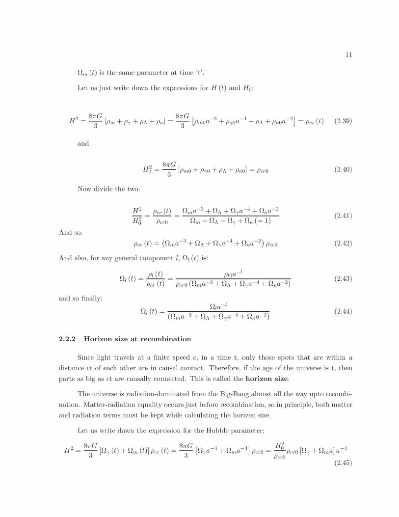
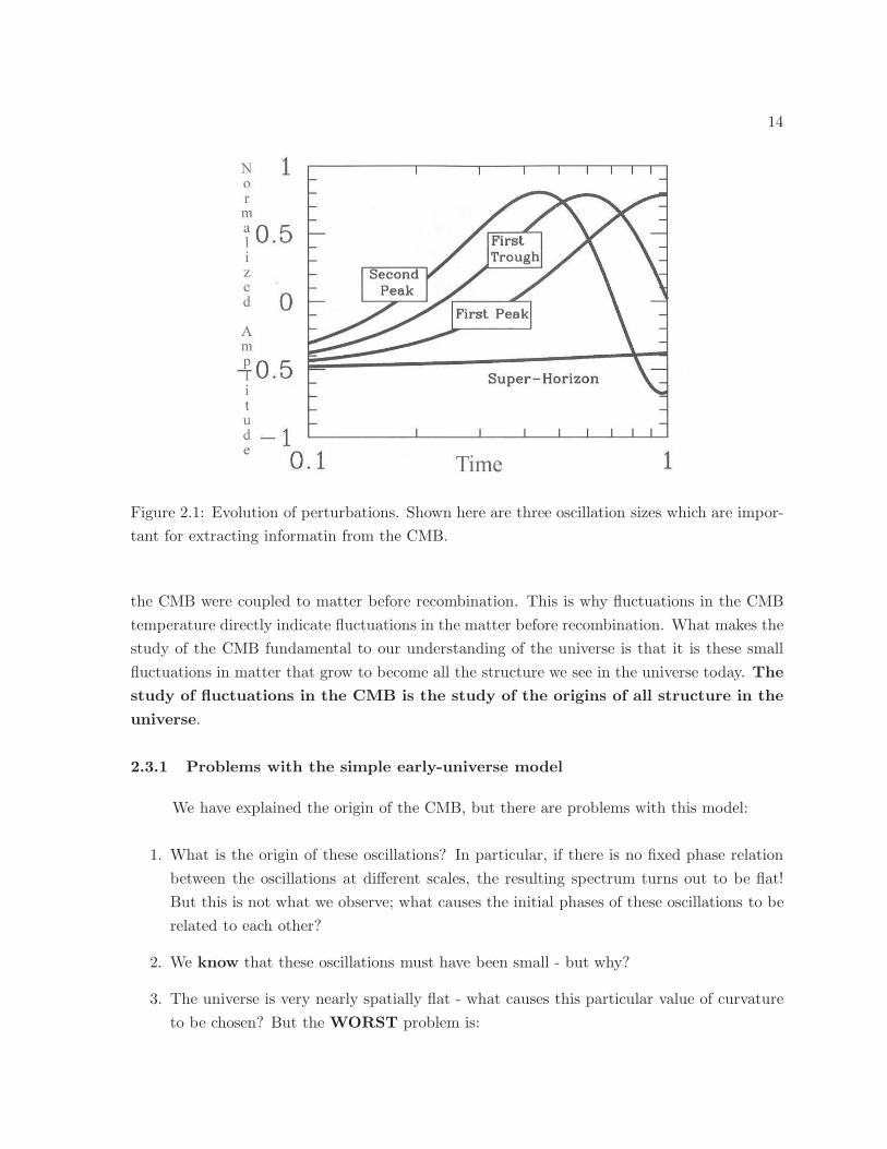
2.1 Evolution of perturbations. Shown here are three oscillation sizes which are
important for extracting informatin from the CMB. . . . . . . . . . . . . . . . . . 14
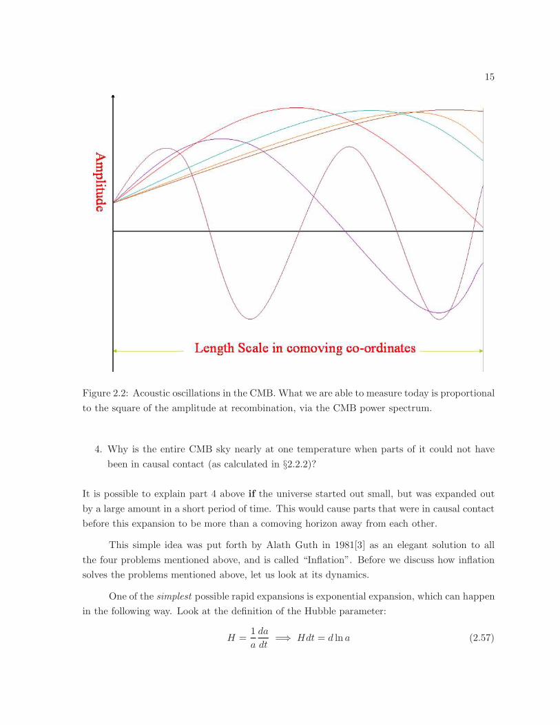
2.2 Acoustic oscillations in the CMB. What we are able to measure today is pro-
portional to the square of the amplitude at recombination, via the CMB power
spectrum. . . . . . . . . . . . . . . . . . . . . . . . . . . . . . . . . . . . . . . . . 15
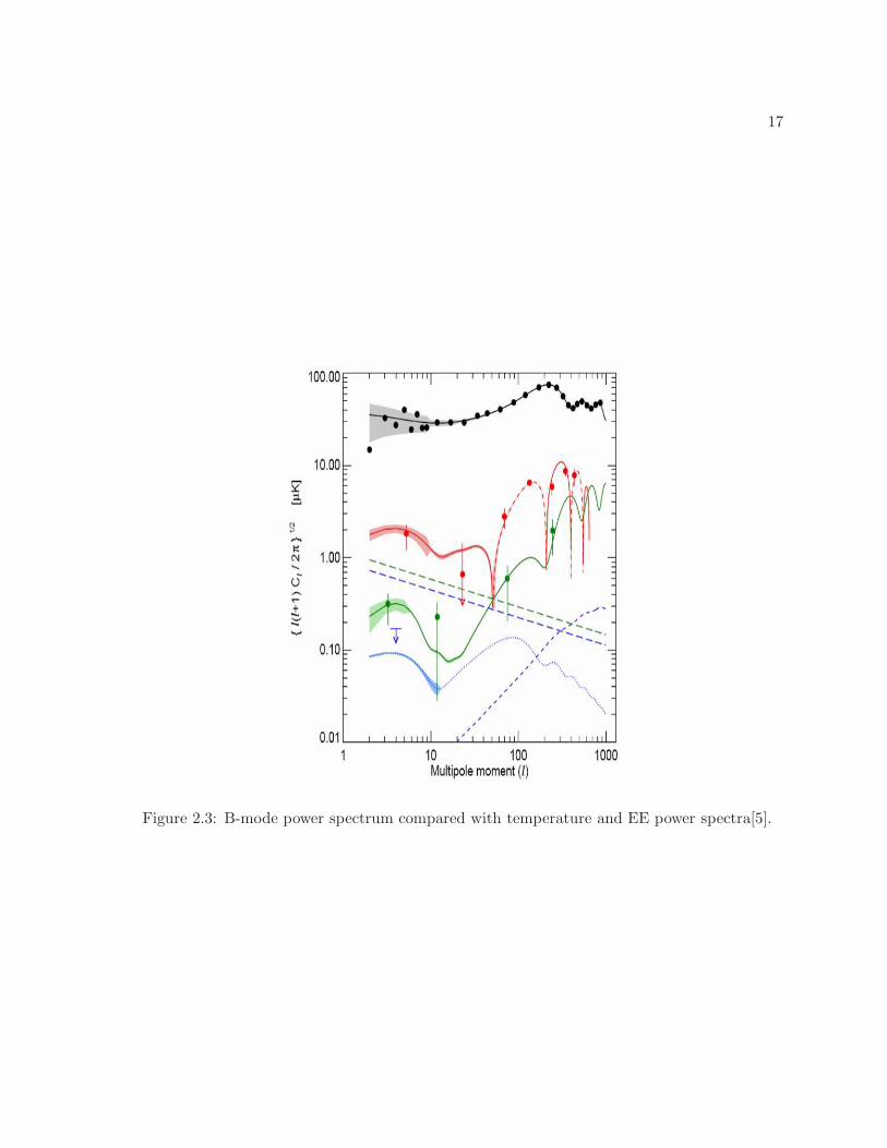
2.3 B-mode power spectrum compared with temperature and EE power spectra[5]. . 17
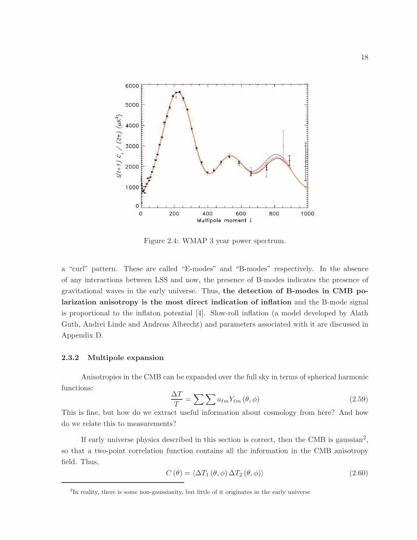
2.4 WMAP 3 year power spectrum. . . . . . . . . . . . . . . . . . . . . . . . . . . . . 18
3.1 B-mode level compared with the levels of E-modes, foregrounds and the lensing
contribution to B-modes[7] . . . . . . . . . . . . . . . . . . . . . . . . . . . . . . 31
3.2 Scalar and Tensor modes with corresponding E and B components. . . . . . . . . 32
3.3 The contribution of tensor modes to the temperature power spectrum (in green). 32
3.4 WMAP 1st year power spectrum, showing cosmic variance at low ℓs. Notice
that the cosmic variance shown here is significantly larger than the tensor mode
contribution in fig.(3.3) . . . . . . . . . . . . . . . . . . . . . . . . . . . . . . . . 33
4.1 A schematic of a bolometer, showing how it works. . . . . . . . . . . . . . . . . . 36
4.2 A schematic of how a bolometer is used. . . . . . . . . . . . . . . . . . . . . . . . 37
4.3 WMAP parameters. . . . . . . . . . . . . . . . . . . . . . . . . . . . . . . . . . . 38
5.1 A general interferometric setup . . . . . . . . . . . . . . . . . . . . . . . . . . . . 43
5.2 One baseline . . . . . . . . . . . . . . . . . . . . . . . . . . . . . . . . . . . . . . 44
5.3 Schematic of interferomentric observation - one baseline. The two antennas are
at G and D. . . . . . . . . . . . . . . . . . . . . . . . . . . . . . . . . . . . . . . . 49
xiv
5.4 The u-v plane coverage of an imager and an interferometer. Figure courtesy Dr.
Carolina Calderon[2]. . . . . . . . . . . . . . . . . . . . . . . . . . . . . . . . . . . 50
5.5 The u-v plane with several pixels. Pixels marked “1” and “2” have the same
distance from the origin, but differ only in their angular position (this corresponds
to the phase of the fringe). Pixels marked “3” and “4” differ in their distance
from the origin and angular position. . . . . . . . . . . . . . . . . . . . . . . . . . 51
5.6 FOV and pixel in the image plane. In this figure and the one alongside, red
represents a pixel in image space and green the FOV in image space. . . . . . . . 52
5.7 The same FOV and pixel as in the previous figure. The size of the interferometer’s
FOV determines its resolution in u-v space. Notice that the two objects have
swapped their dimensions. If N pixels fit in the FOV in the image plane, then
the u-v plane is also divided into N pixels whose size is inversely proportional to
the FOV. . . . . . . . . . . . . . . . . . . . . . . . . . . . . . . . . . . . . . . . . 52
5.8 Adding interferometer. At antenna A2 the electric field is E0, and at A1 it is
E0eiφ, where φ = kB sinα and k = 2π/λ. B is the length of the baseline, and
α is the angle of the source with respect to the symmetry axis of the baseline,
as shown. (For simplicity consider only one wavelength, λ, and ignore time
dependent factors.) In a multiplying interferometer the in-phase output of the
correlator is proportional to E20 cosφ. For the adding interferometer, the output
is proportional to E20 + E2
0 cos(φ + ∆φ(t)). Modulation of ∆φ(t) allows the
recovery of the interference term, E20 cosφ, which is proportional to the visibility
of the baseline. . . . . . . . . . . . . . . . . . . . . . . . . . . . . . . . . . . . . . 66
5.9 Block diagram of a planned CMB polarization experiment. Light enters the
instrument from the left. Each phase switch is modulated in a sequence that
allows recovery of the interference terms (visibilities) by phase-sensitive detec-
tion at the detectors. The signals are mixed in the beam combiner and detected
on cold bolometers at the right. The beam combiner can be implemented either
using guided waves (Butler combiner, as shown here) or quasioptically (Fizeau
combiner, see below). The triangles represent corrugated conical horn antennas,
which connect through transitions to rectangular waveguide. Orthomode trans-
ducers (OMTs) allow all the Stokes parameters to be determined simultaneously. 66
6.1 A simple multi-slit diffraction/interference experiment. Phase differences occur
after light has passed through the slit, inside the instrument. . . . . . . . . . . . 69
xv
6.2 A simple traditional interferometer. Rays suffer phase differences before they
enter the slits. . . . . . . . . . . . . . . . . . . . . . . . . . . . . . . . . . . . . . . 70
6.3 A simple 1-d Fizeau system. Notice that there are two sets of phase differences. . 71
6.4 2-slit diffraction pattern. The large envelope is caused by the single-slit diffrac-
tion and the fine features by the interference between 2 slits. . . . . . . . . . . . 72
6.5 8-slit diffraction pattern. The pattern is more “focused”, leading to better image
recovery. . . . . . . . . . . . . . . . . . . . . . . . . . . . . . . . . . . . . . . . . . 72
6.6 16-slit diffraction pattern, source 10 away from center. . . . . . . . . . . . . . . 72
6.7 16-slit diffraction pattern, source 20 away from center. . . . . . . . . . . . . . . 72
6.8 The u-v plane coverage of one baseline of an interferometer for a single pointing
in a single baseline orientation angle. The two causes of spread in a single pixel
in the u-v plane are shown. Also shown is the size of the FOV, which is the
fundamental limit to u-v resolution. . . . . . . . . . . . . . . . . . . . . . . . . . 73
6.9 The u-v coverage of a single baseline has been divided into many pixels; however,
the beam of a single antenna is larger than a single pixel, so that this division is
not physical. . . . . . . . . . . . . . . . . . . . . . . . . . . . . . . . . . . . . . . 80
7.1 A schematic of the main parts of the MBI instrument. . . . . . . . . . . . . . . . 83
7.2 A schematic of the main parts of the MBI instrument. . . . . . . . . . . . . . . . 84
7.3 A detailed schematic/view of how the Fizeau combiner system fits inside the
MBI instrument. . . . . . . . . . . . . . . . . . . . . . . . . . . . . . . . . . . . . 85
7.4 CMB foreground spectra from the WMAP team [2]. The frequency range of MBI
is indicated by the last yellow column on the right marked “W” for the W-band,
which is very close to the minimum of the combined foreground spectrum. This
is the frequency band in which the MBI operates. . . . . . . . . . . . . . . . . . . 86
7.5 The antenna arrangement (right) and how it looks from atop the cryostat, covered
by filters. . . . . . . . . . . . . . . . . . . . . . . . . . . . . . . . . . . . . . . . . 87
7.6 (a) Simulation of fringe patterns formed in the focal plane of the Fizeau beam
combiner from a single baseline.(b) Superposition of fringes from 6 baselines (as
expected in MBI). Fringes are separated by phase modulation sequence. . . . . . 88
7.7 A spider-web JPL bolometer, with NTD germanium thermistor. . . . . . . . . . 89
7.8 The MBI mount. . . . . . . . . . . . . . . . . . . . . . . . . . . . . . . . . . . . . 90
xvi
7.9 The Vector Network Analyzer(VNA) at the van der Weide lab at UW-Madison.
The FRM is inside the gold cryostat. . . . . . . . . . . . . . . . . . . . . . . . . . 92
7.10 Rotation angle and how it is related to S21 . . . . . . . . . . . . . . . . . . . . . 93
7.11 Rotation angle vs. current, corrected for Ferrite loss, as described in the text. . . 100
7.12 The WR-10 to 0.2” transition (gold) connected with an adapter which then
connects to the circular copper tube. . . . . . . . . . . . . . . . . . . . . . . . . . 101
7.13 Schematics of the planned antenna beam test. . . . . . . . . . . . . . . . . . . . . 101
7.14 Raw data from the tube test for pipes of different lengths. The oscillations are
caused by standing waves in the pipes. Notice that the signal from different
lengths decreases monotonically with increasing length. . . . . . . . . . . . . . . 102
7.15 The same data as in fig.(7.14), but with resonances smoothed out. . . . . . . . . 103
7.16 Graph of loss per 10 feet derived from smoothed data. . . . . . . . . . . . . . . . 104
7.17 Resonances in the data in a small frequency range. These are consistent with
standing waves in the tube lengths used. . . . . . . . . . . . . . . . . . . . . . . . 105
8.1 The power spectrum used to generate the simulated maps shown below. This
was obtained by choosing a set of cosmological parameters in CMBFAST[1]. . . . 109
8.2 The temperature map obtained from the power spectrum above and the method
described in this chapter. The size of the map is in degrees, indicated on the two
axes. Temperatures are in K. . . . . . . . . . . . . . . . . . . . . . . . . . . . . . 110
8.3 Q map obtained from the power spectrum above and the method described in
this chapter. . . . . . . . . . . . . . . . . . . . . . . . . . . . . . . . . . . . . . . . 111
8.4 The temperature map obtained from the power spectrum above and the method
described in this chapter. . . . . . . . . . . . . . . . . . . . . . . . . . . . . . . . 111
8.5 The temperature map that a 6-baseline ideal interferometer is expected to output,
given the sky map shown in fig.(8.2). . . . . . . . . . . . . . . . . . . . . . . . . . 112
8.6 This is a basic check of the map in fig.(8.2). The curves on the top and bottom
indicate the 1-σ error bars expected from eq.(8.6), and the marked points make
up the recovered power spectrum. Note that the vertical scale is different from
the power spectrum in fig.(8.1). . . . . . . . . . . . . . . . . . . . . . . . . . . . . 113
8.7 Schematic of the Quasioptical beam combination set-up inside the cryostat . . . 122

xvii
8.8 Schematic of the Quasioptical beam combination set-up inside the cryostat . . . 123
8.9 The power spectrum used for the simulation. . . . . . . . . . . . . . . . . . . . . 126
8.10 Temperature map from the power spectrum shown in fig.(8.9) above. Used as
input for the instrument simulation. Temperature anisotropies are in µK. . . . . 127
8.11 Recovered power spectrum from the Fizeau system simulation. . . . . . . . . . . 128
9.1 Results from Gibbs’ sampling for the experiment mentioned above. . . . . . . . . 141
9.2 Simulated “flat-sky” CMB map. . . . . . . . . . . . . . . . . . . . . . . . . . . . 148
9.3 The power spectrum used for map simulation and the spectrum recovered from
the simulated map. . . . . . . . . . . . . . . . . . . . . . . . . . . . . . . . . . . . 149
9.4 Estimates of Cℓ recovered from Gibbs’ sampling; beam effects not included. . . . 150
9.5 Map recovered from Gibbs’ sampling, no beam. . . . . . . . . . . . . . . . . . . . 151
9.6 Estimates of Cℓ recovered from Gibbs’ sampling; beam effects included - I. . . . . 152
9.7 Estimates of Cℓ recovered from Gibbs’ sampling; beam effects included - II. . . . 153
9.8 Map recovered from Gibbs’ sampling, beam included - I. . . . . . . . . . . . . . . 154
9.9 Map recovered from Gibbs’ sampling, beam included - II. . . . . . . . . . . . . . 155
9.10 Histograms of recovered values of Cℓs: beam NOT included. . . . . . . . . . . . . 156
B.1 Scematic of the 2-port device . . . . . . . . . . . . . . . . . . . . . . . . . . . . . 167
C.1 Stereographic projection . . . . . . . . . . . . . . . . . . . . . . . . . . . . . . . . 171
1
Chapter 1
Overview
We present here a brief overview of this thesis, followed by an overview of the author’s specific
contributions to the MBI project as described in this thesis.
1.1 Thesis overview
In Chapter 2, we introduce cosmology and build up on first principles to get to the
Friedmann equation. An overview of the physics behind anisotropies in the CMB is given,
followed by a discussion of the serious problems in the model of the early universe, and inflation
is presented as a possible and logical solution to all of these problems. Observable signatures
of inflation on CMB polarization are mentioned.
In Chapter 3, we discuss a way to analyze CMB polarization using spin-harmonics, a
technique reviewed by Wandelt et al [1]. It is shown heuristically that the existence of B-modes
implies the existence of gravitational waves in the early universe, which had their origins in the
inflationary era.
In Chapter 4, we discuss the current state of CMB polarization experiments and briefly
discuss problems with imaging experiments. This leads into a discussion of interferometry and
its merits in Chapter 5. Chapter 6 discusses a novel idea for beam combination that yields
spectral information in fourier space, unlike traditional interferometric systems.
Chapter 7 is an overview of the MBI instrument. Chapter 8 discusses sky and instrument
simulations. Data analysis techniques are discussed in Chapter 9.
1.2 Contributions
MBI is a collaboration between several institutions, UW-Madison, and Brown and Cardiff
Universities being the largest contributors in terms of manpower and resources. MBI’s mount
2
has been designed and built at UW-Madison by Peter Hyland. Tests of MBI’s tracking ability
are ongoing and have so far proven successful. The cryostat was built by Lucio Piccirillo and
tested extensively at Cardiff by Carolina Calderon. Corrugated antennae were tested at Brown
and UW-Madison by Andrei Korotkov and Melissa Lucero. The Fizeau beam combiner was
conceived and designed by Peter Timbie, Gregory Tucker, Lucio Piccirillo and Andrei Korotkov
and has been tested extensively at Brown by Andrei Korotkov. Spider-web bolometers have
been provided by JPL and have been tested at Brown by AK. Faraday effect phase modulators
have been provided by Brian Keating at UCSD. These devices have undergone tests at UW-
Madison, done mostly by Amanda Gault, with support from the author and Peter Hyland.
Evan Bierman at UCSD has provided expert knowledge necessary to carry out these tests.
MBI started out with a Butler beam combiner. Analysis of simulated data from the
Butler version of MBI and extraction of bandpowers have been discussed in exquisite detail
in C. Calderon’s thesis [2]. CC has also studied non-linear methods to recover images from
incomplete u-v coverage. Jaiseung Kim provided the antenna placement that maximizes u-v
coverage.
The author’s main contributions MBI is a unique instrument: it is able to function
simultaneously as an imager and an interferometer. The realization that the MBI is capable of
this is a novel idea that has been introduced in this thesis. Also, simulation and analysis tech-
niques developed in this thesis greatly enhance the capability of this instrument and will allow
exquisite control of systematic effects and in future versions of MBI-4, the ability to characterize
foregrounds - the most important step towards B-mode detection and characterization. With
these as the broad aims of this thesis, the specific contributions of the author are as follows:
1. Chapter 6: The Fizeau combiner system is developed and its application to interferometry
to recover spectral information in the fourier plane, as well as the possibility of operating
an instrument with the Fizeau system as an imager and an interferometer simultaneously
are discussed in detail.
2. Chapter 7:
(a) A measurement of loss in an overmoded circular waveguide system, with a view to
testing antenna beam patterns for MBI.
(b) Characterization of a ferrite-based phase modulator in the W-band (with Amanda
Gault).
(c) Plans to carry out tests of antenna beam patterns once tests described in 2a above
are complete.
3. Chapter 8:
3
(a) Simulation of a CMB sky patch - this was done with a lot of help from Carolina
Calderon.
(b) Simulation of the MBI instrument (specifically the Fizeau system) and crude power
spectrum recovery.
4. Chapter 9: Gibbs’ sampling is a robust, computationally efficient data analysis technique
and is the only efficient method that allows global inference of covariance. This has been
applied to imaging before [3, 4], and we adapt the technique to use it with interferometric
data. This work has been done with Benjamin Wandelt.
5. Chapter 10: Measurements of losses in microstrip lines with a view to replacing guided
wave systems by a compact beam combination scheme (with R. Pathak). This measure-
ment is mentioned only in passing, since this technique is being developed for future
versions of MBI and space-based interferometeric experiments.
MBI’s novelty lies not just in the fact that it is a new instrument with a novel combination
of interferometry and bolometry, but that its specific design allows it to achieve the capability
of characterizing both the CMB signal and foreground. This thesis explores how this is made
possible through design, instrumentation, simulations and data analysis.
4
Bibliography
[1] Y.-T. Lin and B. D. Wandelt, “A beginner′s guide to the theory of CMB temperature and
polarization power spectra in the line-of-sight formalism,” Astroparticle Physics, vol. 25,
pp. 151–166, Mar. 2006.
[2] C. Calderon, “SIMULATION OF THE PERFORMANCE OF THE MILLIMETRE-WAVE
BOLOMETRIC INTERFEROMETER (MBI) FOR COSMIC MICROWAVE BACK-
GROUND OBSERVATIONS. Ph.D. Thesis, Cardiff.,” Ph.D. Thesis, 2006.
[3] B. D. Wandelt, D. L. Larson, and A. Lakshminarayanan, “Global, exact cosmic microwave
background data analysis using Gibbs sampling,” Phys. Rev. D, vol. 70, no. 8, pp. 083511–+,
Oct. 2004.
[4] B. D. Wandelt, “MAGIC: Exact Bayesian Covariance Estimation and Signal Reconstruction
for Gaussian Random Fields,” ArXiv Astrophysics e-prints, Jan. 2004.
5
Chapter 2
Introduction
- Rig Ved, Mandala I (Translation: The primeval atom gave rise to everything we know
in the universe. However, where did it come from, and if its source is unknown, does there even
exist anyone we can offer prayers to?)
It is only relatively recently (19th century onwards) that scientists have made predictions
about and observations of the early Universe and have come up with a successful paradigm that
explains the observations and reconcile them with physical theories.
Once upon a redshift (c. 1965), two scientists at Bell Labs decided to test their shiny new
antenna by pointing it to different parts of the sky. They ended up with a residual noise with
an equivalent temperature of ∼ 3K and a huge confusion on their hands. The puzzle about the
source of this seemingly uniform source was solved only when physicists at the nearby Princeton
University shared with them their ideas about the origins of the universe. Thus started the field
of CMB cosmology, one which has proved to be even more fundamental to our understanding
of the universe over time.
The rest of this chapter will briefly introduce two of the three “pillars” of Cosmology (we
do not discuss primoridal nucleosynthesis here - see, e.g.[1]), as well as the background in Gen-
eral Relativity and discuss the physics and importance of CMB temperature and polarization
anisotropies and how they can acts as windows to the very early universe.
6
2.1 Hubble’s Law and FRWL Cosmology
In the 1920s[2], Hubble pointed his telescope to a few galaxies and discovered the fact
that each one of them was moving away from us, with a velocity proportional to the distance
between us and the galaxy we’re looking at. Since there is no reason to expect that the Milky
Way is at the centre of the Universe, it is reasonable to extend this result and say that every
galaxy is receding from every other with the same property of recession. This has been checked
with observations as well. It turns out that the formalism for expressing Hubble’s law is simple,
and the idea along with all its results remains the same in the General Theory of Relativity
(GR henceforth) as well as Newtonian mechanics. Clearly, Newtonian mechanics is not up to
the task of dealing with the expanding Universe, for several reasons.
Let us denote by r the physical distance between two galaxies, and by v their relative
velocity. Then, Hubble law says that v ∝ r. We can then write the equation
v = Hr (2.1)
where H is called the Hubble parameter (technically, it should be a “constant”, but we have
tacitly ignored curvature and every other issue associated with GR; H can be thought to en-
compass all these GR effects). We would do well to remember that this expansion is not just a
widening in distance between galaxies, it is a “stretching” of space (space-time, strictly speak-
ing, but the beauty of the presently-accepted Friedmann-Robertson-Walker-Lemaitre (FRWL)
universe model is that one can view “spatial slices” or spatial hypersurfaces at different times; it
is possible that the Universe is not FRWL - there are other solutions to the Einstein equations
that are not homogeneous spatially or temporally, but while that is an active area of research,
everyone in the astrophysics comuunity agrees that FRWL is by far the most likely model that
the Universe obeys). In that case, we can (as a matter of fact, we ought to, as we will see later)
reformulate the picture in the following way. We encode the expansion of the Universe in a
single variable which is a function of time, and define what is called a “comoving” frame of
reference in which the distance between, say, any two given galaxies is a constant, i.e. we are
“viewing” this distance from a pre-defined epoch. There is nothing that prevents us from this
pre-defined epoch to “now” - indeed, this is often a convenient choice as we will see. The vari-
able that encodes the expansion of the Universe is called the “scale-factor”, which we represent
here with a (t). We can then write any given physical distance as
r = a (t)x (2.2)
where x is the comoving distance between the two given points under consideration. The
velocity is v = drdt , meaning that
v =d
dt(a (t)x) = x
da
dt(2.3)
7
where the last equality holds because x (i.e. the comoving distance between between any two
given objects) is fixed by definition. We can then write the Hubble law as
v = xda
dt= Hax = Hr (2.4)
⇒ H =1
a
da
dt(2.5)
This, then, is the most general definition of the Hubble parameter. By calling it a parameter,
we have gotten away with proving this relation for any theory of gravity we might choose to
consider - Newtonian or Einsteinian.
Next, we look at a special case of the FRWL metric, namely, the Minkowski metric in
spherical polar co-ordinates:
ds2 = c2dt2 − a (t)2[dr2 + r2dΩ2
](2.6)
It is more convenient to set c = 1 so that
ds2 = dt2 − a (t)2[dr2 + r2dΩ2
](2.7)
where clearly dΩ2 = dθ2 + sin2 θdφ2. This represents flat space-time only. Let us generalize
this to a space-time with positive curvature, in analogy with a 2-sphere (the object we know
and love as a “sphere”). This is a 3-d surface, so in analogy with the “normal” or 2-d sphere
whose equation is
x2 + y2 + z2 = r2 (2.8)
(where r is the radius of the sphere), we have
x2 + y2 + z2 + w2 = b2 (2.9)
Here, x, y and z are ordinary spatial dimensions, and w can be thought of as a fiducial variable,
whose physical interpretation is that it is a 3-sphere embedded in 4-d space. If we accept this
without much ado, we can go about expressing w completely in terms of r, b etc. in the following
way.
We first rewrite the above equation as
r2 + w2 = b2 ⇒ w2 = b2 − r2 (2.10)
Differentiating this equation, we get
2rdr + 2wdw = 0⇒ dw = −rdrw⇒ dw2 =
r2dr2
w2=
r2dr2
b2 − r2 (2.11)
8
Now, the metric has to be modified to
ds2 = dt2 − a (t)2[dr2 + dw2 + r2dΩ2
](2.12)
Let us evaluate a part of the metric:
dr2 + dw2 = dr2[
1 +r2
b2 − r2]
= dr2[b2 − r2 + r2
b2 − r2]
=dr2
1− r2/b2 (2.13)
The 1b2
in the denominator is reminiscent of curvature, and so we call it exactly that and rewrite
it as k. Combining everything together, we then have
ds2 = dt2 − a (t)2[
dr2
1− kr2 + r2dΩ2
]
(2.14)
where k is curvature. Notice that when k = 0, the FRWL metric reduces to Minkowski, as we
would expect it to.
This method can be applied without loss of generality to negative curvature as well, and
the only difference is that the fiducial variable will satisfy this equation
r2 − w2 = b2 (2.15)
so that we will end up with this metric
ds2 = dt2 − a (t)2[
dr2
1 + kr2+ r2dΩ2
]
(2.16)
We can generalize and write
ds2 = dt2 − a (t)2[
dr2
1− kr2 + r2dΩ2
]
(2.17)
where it is understood that k can take positive and negative values. We can write the metric
another way by substituting√kr = sin
√kχ and working out that
dr = cos√kχdχ (2.18)
⇒ dr2 = cos2√kχdχ2 (2.19)
⇒ dr2 =(1− kr2
)dχ2 (2.20)
⇒ dχ2 =dr2
1− kr2 (2.21)
Substituting for this and for r, we get that the metric is
ds2 = dt2 − a (t)2[
dχ2 +sin2√kχ
kdΩ2
]
(2.22)
9
This excercise is useful because we can immediately extract the Angular Diameter Distance
from the new form of the metric - it is the square root of the factor that multiplies dΩ2:
DA =sin√kχ√k
(2.23)
In the case of flat space-time, k → 0 such that sin√kχ√k→ χ = r which is what we expect.
Having studied the geometrical aspects of the metric, let us now turn our attention
to the dynamics of the Universe. The equations that are derived below are again very useful,
especially in their most general form, and their beauty lies in the fact that though the derivation
has nothing to do with GR, these are the exact same result we would get if we worked with
the Einstein equations instead. The GR approach will be outlined briefly after the following
derivation. Let us start from the first law of thermodynamics:
dU + pdV = 0 (2.24)
where, naturally, U = ρa3, where ρ is the density (total energy density, but this can be simplified
for those epochs when the total energy density is dominated by just one component) and a the
scale factor, which is a function of time. Substituting for U , we get
a3dρ+ 3a2ρda+ 3a2pda = 0 (2.25)
⇒ 3a2da (p+ ρ) = −a3dρ (2.26)
⇒ 3 (p+ ρ)da
a= dρ (2.27)
⇒ 3
(p
ρ+ 1
)da
a=
dρ
ρ(2.28)
Now pρ is what is referred to as the equation of state. It is usually denoted by w in the literature,
so we will follow the convention:
3 (w + 1)da
a=dρ
ρ(2.29)
⇒ d ln ρ
d ln a= 3 (1 + w) (2.30)
This, then, is the most general expression relating ρ and a. Notice that we have not yet made
any assumption about w - it may very well be a function of a, and this equation will still hold.
If we assume a constant equation of state w (as is true for baryonic matter and radiation), we
get a simpler relation:
ρ ∼ a−3(1+w) (2.31)
There is another dynamical equation we can derive with our simplistic approach, but this
one requires a leap of faith on one count. Start out with the classical statement for conservation
of energy1
2mv2 − GMm
r= constant (2.32)
10
where m is the mass of a “particle” and M is the mass of the Universe in the shape of a sphere
of uniform density ρ and M = (4/3) πr3ρ. Changing the above equation to represent quantities
per unit mass, we get1
2v2 − 4πG
3
r3ρ
r= constant (2.33)
Use Hubble’s law: v = Hr to get
H2 =8πG
3ρ+
constant
r2(2.34)
This is called the Friedman Equation. It is one of the most fantastic coincidences of Cosmology
that a line of argument as weak as the preceding one can yield the same result as GR. We
can derive this from Einstein’s Equations, with the only difference that the second term on the
right will be − kr2
where k is space-time curvature, as before, so that the final equation is
H2 =8πG
3ρ− k
r2(2.35)
2.2 Cosmodynamic calculations
Having introduced the basic concepts in cosmology, let us work through a few small
calculation that will be relevant in §2.3. It is conventional to write eq.(2.35) as
H2 =8πG
3ρcrit (2.36)
where we have incorporated curvature and the net energy density of the universe in the quantity
ρcrit. When studying cosmology, we are not always interested in the value of ρ for different
components - just what fraction of the energy density they make up. To this end, we define a
set of parameters denoted by Ω such that for a component X,
ΩX =ρXρcrit
(2.37)
is the fraction of energy density in component X at a given time.
2.2.1 Preliminaries
Here is my notation: m,γ,Λ, κ denote matter, radiation, vacuum and curvature respec-
tively.
Ωm = Ωm,NOW = Ωm0 (2.38)
etc., and
11
Ωm (t) is the same parameter at time ’t’.
Let us just write down the expressions for H (t) and H0:
H2 =8πG
3[ρm + ργ + ρΛ + ρκ] =
8πG
3
[ρm0a
−3 + ργ0a−4 + ρΛ + ρκ0a
−2]
= ρcr (t) (2.39)
and
H20 =
8πG
3[ρm0 + ργ0 + ρΛ + ρκ0] = ρcr0 (2.40)
Now divide the two:
H2
H20
=ρcr (t)
ρcr0=
Ωma−3 + ΩΛ + Ωγa
−4 + Ωκa−2
Ωm + ΩΛ + Ωγ + Ωκ (= 1)(2.41)
And so:
ρcr (t) =(Ωma
−3 + ΩΛ + Ωγa−4 + Ωκa
−2)ρcr0 (2.42)
And also, for any general component l, Ωl (t) is:
Ωl (t) =ρl (t)
ρcr (t)=
ρl0a−l
ρcr0 (Ωma−3 + ΩΛ + Ωγa−4 + Ωκa−2)(2.43)
and so finally:
Ωl (t) =Ωla
−l
(Ωma−3 + ΩΛ + Ωγa−4 + Ωκa−2)(2.44)
2.2.2 Horizon size at recombination
Since light travels at a finite speed c, in a time t, only those spots that are within a
distance ct of each other are in causal contact. Therefore, if the age of the universe is t, then
parts as big as ct are causally connected. This is called the horizon size.
The universe is radiation-dominated from the Big-Bang almost all the way upto recombi-
nation. Matter-radiation equality occurs just before recombination, so in principle, both matter
and radiation terms must be kept while calculating the horizon size.
Let us write down the expression for the Hubble parameter:
H2 =8πG
3[Ωγ (t) + Ωm (t)] ρcr (t) =
8πG
3
[Ωγa
−4 + Ωma−3]ρcr0 =
H20
ρcr0ρcr0 [Ωγ + Ωma] a
−4
(2.45)
12
Replacing H20 by 100 km
sMpc , we get:
H =√
[Ωγ + Ωma]a−2h
(
100km
sMpc
)
(2.46)
Now we get to what we started out to calculate, the horizon size at recombination:
ηR = c
∫ a=10−3
a=0
dt
a= c
∫ 10−3
0
da
a2H(2.47)
Replacing the value of H from above, we get:
ηR =c
100
∫ 10−3
0
da√
(Ωγ + Ωma)hMpc =
3000Mpc
(Ωmh2)12
∫ 10−3
0
da√(
Ωγ
Ωm+ a) (2.48)
The final result is:
ηR =6000
(Ωmh2)12
(√
Ωγ
Ωm+ 10−3 −
√
Ωγ
Ωm
)
(2.49)
Putting in Ωm=0.3, Ωγ = 4.8× 10⁻⁵ and h=0.72, we get ηR= 326 Mpc. This is the comoving
horizon size at recombination. Considering the age of the universe to be ∼14G light years, we
get that the angle that the horizon subtends on the sky should be
θrecombination horizon =326
14000× 3.26 ≈ 4.3 (2.50)
This means that only 4.3 patches should have similar temperatures on the sky! However, this
is not true - the CMB sky is very nearly uniform. This problem is discussed further in §2.3.1.
In the foregoing calculation, we have assumed that information is able to travel at the
speed of light. However, in reality, information travels at the speed of sound in the plasma,
which happens to be ∼ c√3, so that the above estimate revises to ∼2.
2.2.3 Age of the Universe
From eq. 4, we have
H2 = H20
[ρcr (t)
ρcr0
]
= H20
[Ωma
−3 + ΩΛ + Ωγa−4 + Ωκa
−2
Ωm + ΩΛ + Ωγ + Ωκ (= 1)
]
(2.51)
and so
H = H0
[Ωma
−3 + ΩΛ + Ωγa−4 + Ωκa
−2] 1
2 (2.52)
Remember the definition of the Hubble parameter:
H =1
a
da
dt(2.53)
13
from where
dt =da
aH=
da
aH0 [Ωma−3 + ΩΛ + Ωγa−4 + Ωκa−2]12
(2.54)
so that
t =
∫da
aH=
∫da
aH0 [Ωma−3 + ΩΛ + Ωγa−4 + Ωκa−2]12
(2.55)
is a general expression for the age of the universe, without quintessence. Now, a = 11+z so that
da = − dz(1+z)2
so that
t = −∫
dz
(1 + z)H0
[
Ωm (1 + z)3 + ΩΛ + Ωγ (1 + z)4 + Ωκ (1 + z)2] 1
2
(2.56)
2.3 The CMB
The CMB is another “pillar” of cosmology, and by far the most informative one. Before
we delve into what cosmological parameters can be constrained with the CMB, let us look
briefly at the CMB itself.
Hubble’s law imples that as we go back in time, the size of the universe decreases mono-
tonically. This means that the wavelength of photons decreases and the temperature of the
universe increases. This implies that there must have been an epoch earlier than which the
universe would have been ionized. This epoch is called “recombination” or “last scattering
surface” and we shall use these terms interchangably. Before recombination, the universe can
be thought of as a “primordial soup” of protons, electrons, neutrons (i.e. baryonic matter) and
photons. Baryonic matter experiences two opposing forces: the attractive force of gravity and
repulsive force of radiation pressure. These two opposing forces set up acoustic oscillations in
the “primordial soup”. But these end at recombination, and the photons that travel freely after
recombination constitute the CMB. We need to remember, though, that the universe is expand-
ing even as these acoustic oscillations permeate the universe. Keeping this in mind, and looking
at comoving distances instead of physical ones, let us examine the acoustic oscillations in a little
more detail. Ignoring the origin of the oscillations for the moment, we immediately see from
figs.(2.1) and (2.2) that every length scale ends up with a different amplitude. If the wavelength
of a “mode” (i.e. a length scale) is sufficiently large, small changes in the wavelength do not
produce an appreciable effect (this is the reason that the power spectrum is nearly constant
for low ℓs - see fig.(2.4)). As the wavelength decreases, however, the amplitude of the mode at
recombination increases until it reaches a maximum, and then decreases with decreasing wave-
length. The amplitude cannot possibly be measured today, but the power level can, and so this
is the quantity that CMB cosmology aims to measure. The reason that we can measure this
quantity (i.e. the power in fluctuations in matter) is that the photons that we detect today as
14
Figure 2.1: Evolution of perturbations. Shown here are three oscillation sizes which are impor-
tant for extracting informatin from the CMB.
the CMB were coupled to matter before recombination. This is why fluctuations in the CMB
temperature directly indicate fluctuations in the matter before recombination. What makes the
study of the CMB fundamental to our understanding of the universe is that it is these small
fluctuations in matter that grow to become all the structure we see in the universe today. The
study of fluctuations in the CMB is the study of the origins of all structure in the
universe.
2.3.1 Problems with the simple early-universe model
We have explained the origin of the CMB, but there are problems with this model:
1. What is the origin of these oscillations? In particular, if there is no fixed phase relation
between the oscillations at different scales, the resulting spectrum turns out to be flat!
But this is not what we observe; what causes the initial phases of these oscillations to be
related to each other?
2. We know that these oscillations must have been small - but why?
3. The universe is very nearly spatially flat - what causes this particular value of curvature
to be chosen? But the WORST problem is:
15
Figure 2.2: Acoustic oscillations in the CMB. What we are able to measure today is proportional
to the square of the amplitude at recombination, via the CMB power spectrum.
4. Why is the entire CMB sky nearly at one temperature when parts of it could not have
been in causal contact (as calculated in §2.2.2)?
It is possible to explain part 4 above if the universe started out small, but was expanded out
by a large amount in a short period of time. This would cause parts that were in causal contact
before this expansion to be more than a comoving horizon away from each other.
This simple idea was put forth by Alath Guth in 1981[3] as an elegant solution to all
the four problems mentioned above, and is called “Inflation”. Before we discuss how inflation
solves the problems mentioned above, let us look at its dynamics.
One of the simplest possible rapid expansions is exponential expansion, which can happen
in the following way. Look at the definition of the Hubble parameter:
H =1
a
da
dt=⇒ Hdt = d ln a (2.57)
16
Exponential expansion =⇒ a ∼ econstant×t, which can be easily achieved if H is a constant.
Thus, exponential expansion =⇒ constant H. But what component of the universe can
satisfy this condition? Let us look at the Friedmann equation:
H2 =8πG
3ρ− k
r2=⇒ H ∼ √ρ (2.58)
This means that the energy density of the component dominating the total energy density would
have to be constant. However, from eq.(2.31), we get that ρ can be constant with time if and
only if w = −1, which implies a negative pressure. While the standard model of particle physics
does not provide us with a particle with this property, [4] shows a possible way to get w = −1:
a scalar field that is “slowly rolling” down a potential, such that the potential energy dominates
the kinetic energy at first, but this slowly reverses. Certain criteria need to be satisfied in order
for this to happen, and these are discussed in Appendix E.
Let us now return to the three problems mentioned above and see how inflation can solve
them:
1. Quantum field theory tells us that there must be fluctuations at the level of ∼ 10−30 in
classical vacuum. If these fluctuations in energy density can be expanded out by factors
of ∼ 1025, we get classical fluctuations ∼ 10−5, which can act as seeds for the acoustic
oscillations which lead to the formation of the CMB and large scale structure in the
universe. Furthermore, the spectrum of these fluctuations is flat.
2. Inflation expands EVERY scale by the same factor. Combined with the flatness of the
initial quantum fluctuations, this leads to all the acoustic oscillations starting out in the
same phase.
3. The universe can easily have a non-zero curvature pre-inflation. However, it is always
possible to find a small enough region of space which is spatially flat. Inflation can
expand out this small section to the entire observable universe.
4. As stated before, inflation can get rid of the horizon problem with the correct amount of
expansion.
Inflation doesn’t just solve the problems in early universe cosmology. It produces gravi-
tational waves as well - these are the tensor perturbations in Einstein’s equations of GR in the
early universe[4]. Scattering produces polarization before the LSS because photons have a small
quadrupole moment1. The gravitational wave passing through space-time while polarization
is being produced causes a certain “curl” pattern to be produced [6]. Thus, polarization over
the CMB sky can be split into two parts - one with a “gradient” pattern and the other with
1The reason for this is discussed in detail in chapter 2
17
Figure 2.3: B-mode power spectrum compared with temperature and EE power spectra[5].
18
Figure 2.4: WMAP 3 year power spectrum.
a “curl” pattern. These are called “E-modes” and “B-modes” respectively. In the absence
of any interactions between LSS and now, the presence of B-modes indicates the presence of
gravitational waves in the early universe. Thus, the detection of B-modes in CMB po-
larization anisotropy is the most direct indication of inflation and the B-mode signal
is proportional to the inflaton potential [4]. Slow-roll inflation (a model developed by Alath
Guth, Andrei Linde and Andreas Albrecht) and parameters associated with it are discussed in
Appendix D.
2.3.2 Multipole expansion
Anisotropies in the CMB can be expanded over the full sky in terms of spherical harmonic
functions:∆T
T=∑∑
aℓmYℓm (θ, φ) (2.59)
This is fine, but how do we extract useful information about cosmology from here? And how
do we relate this to measurements?
If early universe physics described in this section is correct, then the CMB is gaussian2,
so that a two-point correlation function contains all the information in the CMB anisotropy
field. Thus,
C (θ) = 〈∆T1 (θ, φ)∆T2 (θ, φ)〉 (2.60)
2In reality, there is some non-gaussianity, but little of it originates in the early universe
19
contains all the information in the CMB. It turns out that the fourier transform of C (θ) is
Cℓδℓℓ′δmm′ = 〈aℓma∗ℓ′m′〉 (2.61)
where Cℓ is known as the power spectrum of the CMB. It tells us the amount of power in
anisotropies at a given lengthscale specified by ℓ, where for large enough ℓ (¿20), ℓ = πθ . For
a detailed discussion of this relationship, see Appendix C. In fig.(2.1), the amplitude of the
oscillation at the LSS is determined by the wavelength of the particular oscillation. Each Cℓ is
the square of the amplitude for a particular value of the wavelength, which is a function of ℓ
and therefore an angle on the sky. This is the reason that a power spectrum is a more
useful tool for studying the early universe than an image - it probes individual angular
scales on the sky and therefore individual length scales in the early universe. We shall discuss
later in §5.6 how the power spectrum is related to the output of an interferometer. The power
spectrum from 3-year WMAP data is shown in fig.(2.4) [5].
20
Bibliography
[1] R. H. Cyburt, B. D. Fields, and K. A. Olive, “Primordial nucleosynthesis with CMB inputs:
probing the early universe and light element astrophysics,” Astroparticle Physics, vol. 17,
pp. 87–100, Apr. 2002.
[2] E. Hubble, “A Relation between Distance and Radial Velocity among Extra-Galactic Neb-
ulae,” Proceedings of the National Academy of Science, vol. 15, pp. 168–173, Mar. 1929.
[3] A. H. Guth, “Inflationary universe: A possible solution to the horizon and flatness prob-
lems,” Phys. Rev. D, vol. 23, pp. 347–356, Jan. 1981.
[4] S. Dodelson, Modern cosmology, Modern cosmology / Scott Dodelson. Amsterdam (Nether-
lands): Academic Press. ISBN 0-12-219141-2, 2003, XIII + 440 p., 2003.
[5] L. Page, G. Hinshaw, E. Komatsu, M. R. Nolta, D. N. Spergel, C. L. Bennett, C. Barnes,
R. Bean, O. Dore, J. Dunkley, M. Halpern, R. S. Hill, N. Jarosik, A. Kogut, M. Limon, S. S.
Meyer, N. Odegard, H. V. Peiris, G. S. Tucker, L. Verde, J. L. Weiland, E. Wollack, and
E. L. Wright, “Three-Year Wilkinson Microwave Anisotropy Probe (WMAP) Observations:
Polarization Analysis,” ApJ Suppl., vol. 170, pp. 335–376, June 2007.
[6] W. Hu and M. White, “A CMB polarization primer,” New Astronomy, vol. 2, pp. 323–344,
Oct. 1997.
21
Chapter 3
Theory of CMB Polarization
Most of the discussion in this chapter can be found in [1] and [2].
A monochromatic plane electromagnetic wave is characterized in the following way. The
x and y components of both E and H fields obey the wave equation. If the direction of
propagation is z, then the electric fields are given by
Ex = Ex0ei(kz−ωt+δx)
Ey = Ey0ei(kz−ωt+δy) (3.1)
where δx and δy are phases associated with the two components.
Despite the appearance of 4 variables, there really are only 3 independent ones in the
above equations: Ex0, Ex0 and δ = δy − δx. We therefore need 3 quantities to completely
characterize a monochromatic wave. The extension to quasi-monochromatic waves is discussed
in §3.1 - it will emerge there that we need 4, and not 3 parameters to completely characterize
a general wave.
Even though Ex0, Ey0 and δ = δy − δx completely characterize a monochromatic wave,
this parametrization/characterization is not satisfactory, because none of these quantities can
be directly measured by an instrument. Instruments can measure |Ex0|2, |Ey0|2 or their linear
combinations. For instance, it is possible to use waveguides and detectors to separate out and
measure |Ex0|2 and |Ey0|2 for this wave. We therefore need 3 parameters in terms of |Ex0|2 and
|Ey0|2 which contain all information about Ex0, Ey0 and δ = δy − δx.
Simultaneously, we need to describe the state of polarization of the wave. These two prob-
lems are tightly coupled, and can be solved simultaneously as follows. One obvious parameter
is the total intensity of the wave, I = |Ex0|2 + |Ey0|2, or equivalently, I = Ix+Iy, which is easily
measured by total-power detectors. Next, thinking only in terms of linear polarization, we can
define polarization as a “difference in intensity along two independent axes”. The preceding
22
sentence is strictly speaking, wrong, since I is a scalar. But it does make sense to compare
|Ex0|2 and |Ey0|2 to check if there is more power on one axis than the other. But this “extra
power along one axis” is precisely the definition of polarization! We can therefore define one
polarization parameter in the following way
Q = |Ex0|2 − |Ey0|2 (3.2)
We need to check what happens to Q under a rotation, since it is not guaranteed to be a
rotation-invariant quantity. We do this as follows.
Under a rotation by an angle, say θ, co-ordinates transform as
x′ = x cos θ + y sin θ
y′ = −x sin θ + y cos θ (3.3)
Electric fields will therefore transform the same way:
E′x = Ex cos θ + Ey sin θ
E′y = −Ex sin θ + Ey cos θ (3.4)
In the rotated co-ordinate system, Stokes’ Q is
Q′ = |E′x|2 − |E′
y|2 (3.5)
and
|E′x|2 = (Ex cos θ + Ey sin θ)
(E∗x cos θ + E∗
y sin θ)
|E′y|2 = (−Ex sin θ + Ey cos θ)
(−E∗
x sin θ +E∗y cos θ
)(3.6)
so that
|E′x|2 = |Ex|2 cos2 θ + |Ey|2 sin2 θ + cos θ sin θ
(ExE
∗y
)
|E′y|2 = |Ex|2 sin2 θ + |Ey|2 cos2 θ − cos θ sin θ
(ExE
∗y
)(3.7)
But the quantity in the last bracket is just 2ℜ (E∗xEy). Subtract the two expressions to get
Q′ =(|Ex|2 − |Ey|2
) (cos2 θ − sin2 θ
)+ 2 sin θ cos θ (2ℜ (E∗
xEy)) (3.8)
Using the trigonometric identities, and the definition of Q: Q = |Ex|2 − |Ey|2, we get
Q′ = Q cos 2θ + 2ℜ (E∗xEy) sin 2θ (3.9)
When we compare this to the transformation of co-ordinates above, we find that this equation
suggests that we define a quantity 2R (E∗xEy) - we call this Stokes’ U. We can check that U
transforms as
U ′ = −Q sin 2θ + U cos 2θ (3.10)
23
so that
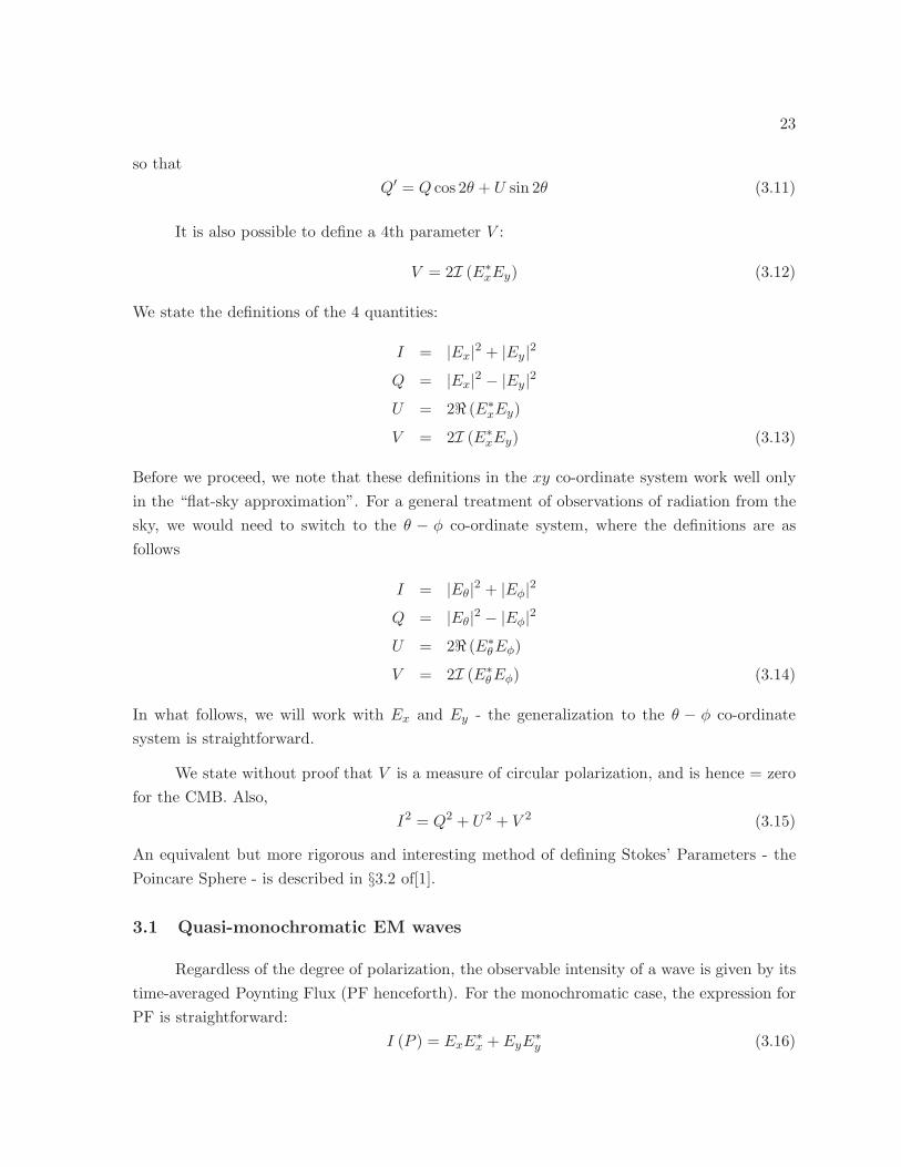
Q′ = Q cos 2θ + U sin 2θ (3.11)
It is also possible to define a 4th parameter V :
V = 2I (E∗xEy) (3.12)
We state the definitions of the 4 quantities:
I = |Ex|2 + |Ey|2
Q = |Ex|2 − |Ey|2
U = 2ℜ (E∗xEy)
V = 2I (E∗xEy) (3.13)
Before we proceed, we note that these definitions in the xy co-ordinate system work well only
in the “flat-sky approximation”. For a general treatment of observations of radiation from the
sky, we would need to switch to the θ − φ co-ordinate system, where the definitions are as
follows
I = |Eθ|2 + |Eφ|2
Q = |Eθ|2 − |Eφ|2
U = 2ℜ (E∗θEφ)
V = 2I (E∗θEφ) (3.14)
In what follows, we will work with Ex and Ey - the generalization to the θ − φ co-ordinate
system is straightforward.
We state without proof that V is a measure of circular polarization, and is hence = zero
for the CMB. Also,
I2 = Q2 + U2 + V 2 (3.15)
An equivalent but more rigorous and interesting method of defining Stokes’ Parameters - the
Poincare Sphere - is described in §3.2 of[1].
3.1 Quasi-monochromatic EM waves
Regardless of the degree of polarization, the observable intensity of a wave is given by its
time-averaged Poynting Flux (PF henceforth). For the monochromatic case, the expression for
PF is straightforward:
I (P ) = ExE∗x + EyE
∗y (3.16)
24
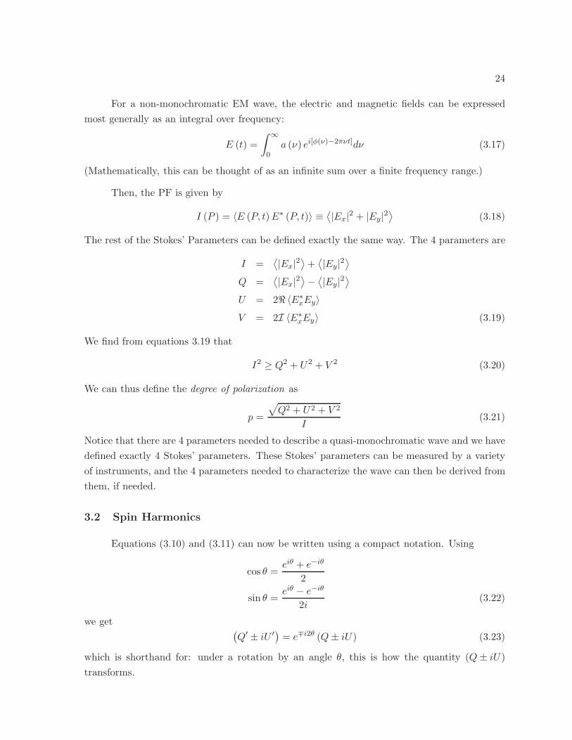
For a non-monochromatic EM wave, the electric and magnetic fields can be expressed
most generally as an integral over frequency:
E (t) =
∫ ∞
0a (ν) ei[φ(ν)−2πνt]dν (3.17)
(Mathematically, this can be thought of as an infinite sum over a finite frequency range.)
Then, the PF is given by
I (P ) = 〈E (P, t)E∗ (P, t)〉 ≡⟨|Ex|2 + |Ey|2
⟩(3.18)
The rest of the Stokes’ Parameters can be defined exactly the same way. The 4 parameters are
I =⟨|Ex|2
⟩+⟨|Ey|2
⟩
Q =⟨|Ex|2
⟩−⟨|Ey|2
⟩
U = 2ℜ 〈E∗xEy〉
V = 2I 〈E∗xEy〉 (3.19)
We find from equations 3.19 that
I2 ≥ Q2 + U2 + V 2 (3.20)
We can thus define the degree of polarization as
p =
√
Q2 + U2 + V 2
I(3.21)
Notice that there are 4 parameters needed to describe a quasi-monochromatic wave and we have
defined exactly 4 Stokes’ parameters. These Stokes’ parameters can be measured by a variety
of instruments, and the 4 parameters needed to characterize the wave can then be derived from
them, if needed.
3.2 Spin Harmonics
Equations (3.10) and (3.11) can now be written using a compact notation. Using
cos θ =eiθ + e−iθ
2
sin θ =eiθ − e−iθ
2i(3.22)
we get(Q′ ± iU ′) = e∓i2θ (Q± iU) (3.23)
which is shorthand for: under a rotation by an angle θ, this is how the quantity (Q± iU)
transforms.
25
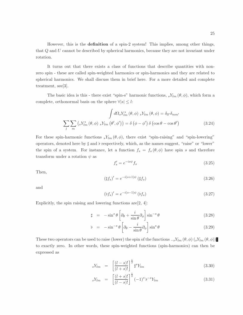
However, this is the definition of a spin-2 system! This implies, among other things,
that Q and U cannot be described by spherical harmonics, because they are not invariant under
rotation.
It turns out that there exists a class of functions that describe quantities with non-
zero spin - these are called spin-weighted harmonics or spin-harmonics and they are related to
spherical harmonics. We shall discuss them in brief here. For a more detailed and complete
treatment, see[3].
The basic idea is this - there exist “spin-s” harmonic functions, sYlm (θ, φ), which form a
complete, orthonormal basis on the sphere ∀|s| ≤ l:∫
dΩsY∗lm (θ, φ) sYlm (θ, φ) = δll′δmm′
∑
l
∑
m
(
sY∗lm (θ, φ) sYlm
(θ′, φ′
))= δ
(φ− φ′
)δ(cos θ − cos θ′
)(3.24)
For these spin-harmonic functions sYlm (θ, φ), there exist “spin-raising” and “spin-lowering”
operators, denoted here by ♯ and respectively, which, as the names suggest, “raise” or “lower”
the spin of a system. For instance, let a function fs = fs (θ, φ) have spin s and therefore
transform under a rotation ψ as
f ′s = e−isψfs (3.25)
Then,
(♯fs)′ = e−i(s+1)ψ (♯fs) (3.26)
and
(fs)′ = e−i(s−1)ψ (fs) (3.27)
Explicitly, the spin raising and lowering functions are[2, 4]:
♯ = − sins θ
[
∂θ +i
sin θ∂φ
]
sin−s θ (3.28)
= − sin−s θ
[
∂θ −i
sin θ∂φ
]
sins θ (3.29)
These two operators can be used to raise (lower) the spin of the functions −sYlm (θ, φ) (sYlm (θ, φ))
to exactly zero. In other words, these spin-weighted functions (spin-harmonics) can then be
expressed as
sYlm =
[(l − s)!(l + s)!
] 12
♯sYlm (3.30)
sYlm =
[(l + s)!
(l − s)!
] 12
(−1)s −sYlm (3.31)
26
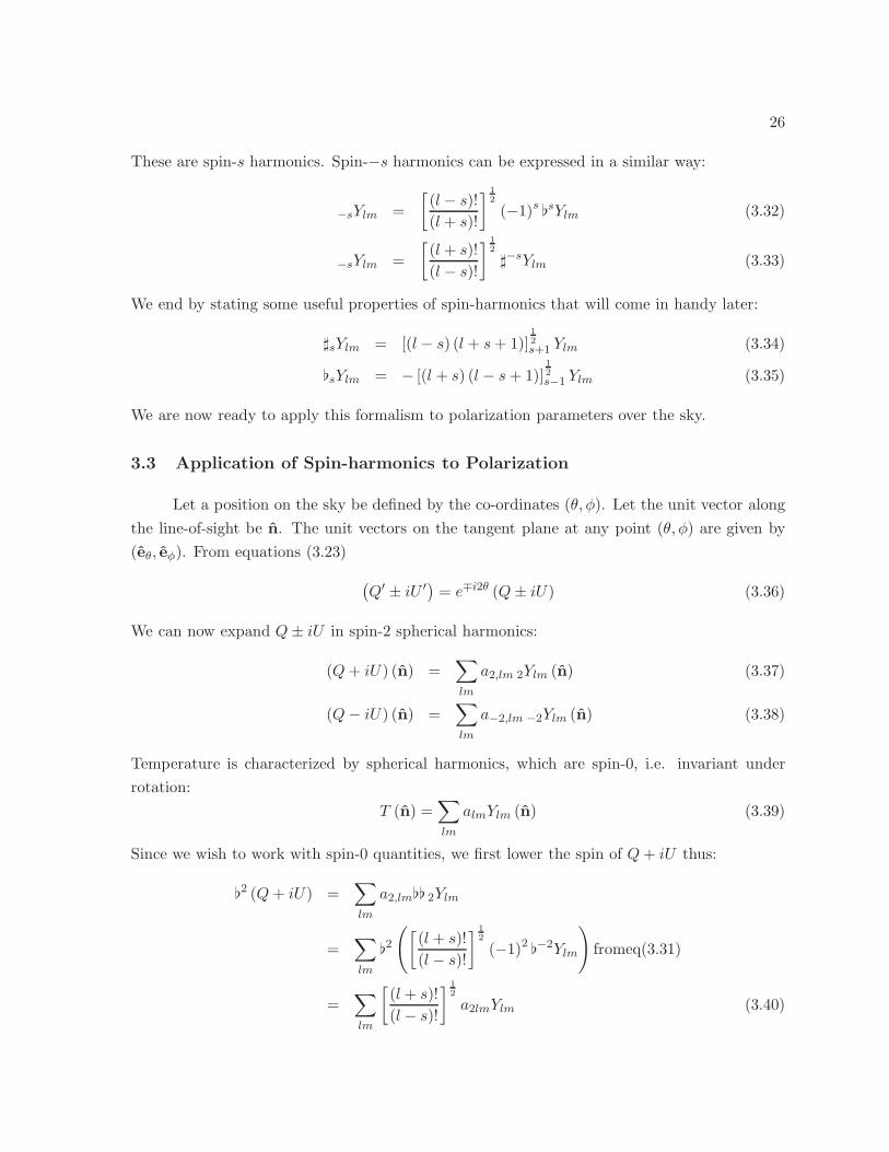
These are spin-s harmonics. Spin-−s harmonics can be expressed in a similar way:
−sYlm =
[(l − s)!(l + s)!
] 12
(−1)s sYlm (3.32)
−sYlm =
[(l + s)!
(l − s)!
] 12
♯−sYlm (3.33)
We end by stating some useful properties of spin-harmonics that will come in handy later:
♯sYlm = [(l − s) (l + s+ 1)]12
s+1 Ylm (3.34)
sYlm = − [(l + s) (l − s+ 1)]12
s−1 Ylm (3.35)
We are now ready to apply this formalism to polarization parameters over the sky.
3.3 Application of Spin-harmonics to Polarization
Let a position on the sky be defined by the co-ordinates (θ, φ). Let the unit vector along
the line-of-sight be n. The unit vectors on the tangent plane at any point (θ, φ) are given by
(eθ, eφ). From equations (3.23)
(Q′ ± iU ′) = e∓i2θ (Q± iU) (3.36)
We can now expand Q± iU in spin-2 spherical harmonics:
(Q+ iU) (n) =∑
lm
a2,lm 2Ylm (n) (3.37)
(Q− iU) (n) =∑
lm
a−2,lm −2Ylm (n) (3.38)
Temperature is characterized by spherical harmonics, which are spin-0, i.e. invariant under
rotation:
T (n) =∑
lm
almYlm (n) (3.39)
Since we wish to work with spin-0 quantities, we first lower the spin of Q+ iU thus:
2 (Q+ iU) =∑
lm
a2,lm 2Ylm
=∑
lm
2
([(l + s)!
(l − s)!
] 12
(−1)2 −2Ylm
)
fromeq(3.31)
=∑
lm
[(l + s)!
(l − s)!
] 12
a2lmYlm (3.40)
27
Similarly,
♯2 (Q− iU) =∑
lm
a−2,lm−2Ylm
=∑
lm
♯2
([(l + s)!
(l − s)!
] 12
♯−2Ylm
)
from eq(3.30)
=∑
lm
[(l + s)!
(l − s)!
] 12
a−2lmYlm (3.41)
Now, since our aim is to work with spin-0 quantities constructed from (Q± iU), we can
in principle work with 2 (Q+ iU) and ♯2 (Q− iU). However, this is not a convenient choice for
the following reason. Q has parity even and U has parity odd, i.e. under a rotation n → −n,
we get Q→ Q, U → −U .
We would, therefore, like to work with two spin-0 quantities with well-defined parities,
i.e. one with parity even and the other with parity odd. However, the two quantities Q± iU do
not have this property, and so we cannot expect the parities of 2 (Q+ iU) and ♯2 (Q− iU) to
work out to be even/odd. We need to construct two other quantities, say E and B from these
two thus:
E = a2 (Q+ iU) + b♯2 (Q− iU) (even) (3.42)
B = c2 (Q+ iU) + d♯2 (Q− iU) (odd) (3.43)
where we need to determine the 4 quantities a, b, c, d.
We can write
E =(a2 + b♯2
)Q+ i
(a2 − b♯2
)U (3.44)
B =(c2 + d♯2
)Q+ i
(c2 − d♯2
)U (3.45)
Thus, we need even parities for a2 + b♯2 and c2 − d♯2 as well as odd parities for a2 − b♯2and c2 + d♯2. But under a parity transformation 2 → (−1)l ♯2 and ♯2 → (−1)l 2. Thus, we
will have all the required parities as required iff a = b and c = −d. In particular, we choose
a = b = −12 and c = −d = 1
2i for reasons of normalization [2]. The expressions for E and B are
E = −1
2
[2 (Q+ iU) + ♯2 (Q− iU)
](even) (3.46)
B =1
2i
[2 (Q+ iU)− ♯2 (Q− iU)
](odd) (3.47)
These are the so-called “E and B-modes” in CMB polarization. The reason for the choice of the
letters E and B is primarily their respective parities: E-modes have parity even, like electric
28
fields, and B-modes have parity odd, like magnetic fields. This relationship between E and
B-modes and Stokes’ parameters is derived in a different way in Appendix E.
E and B-modes can now be expanded in terms of spherical harmonics:
E =∑
lm
aElmYlm (3.48)
B =∑
lm
aBlmYlm (3.49)
where
aElm = −(l + 2)!
(l − 2)!
a2lm + a−2lm
2(3.50)
aBlm = −(l + 2)!
(l − 2)!
a2lm − a−2lm
2(3.51)
We can now define the power spectra that provide a statistical description of CMB tem-
perature and polarization anisotropies:
CXℓ =1
2ℓ+ 1
∑
m
〈a∗XℓmaXℓm〉 (3.52)
where X = T,E,B and 〈· · · 〉 ≡ ensemble average.
Here is another reason for working with E and B-modes instead of 2 (Q+ iU) and
♯2 (Q− iU): since E-modes are parity even and B-modes parity odd, the cross-correlations
BE, BT vanish. This means that we have to deal with fewer power spectra. Had we chosen
2 (Q+ iU) and ♯2 (Q− iU), we would have had to analyze atleast two more power spectra,
without gaining any additional physical insight.
3.4 Thomson Scattering
Scattering of a photon from an electron, when there is no change in photon energy, is
called Thomson scattering. Since electrons (and protons) are free before last scattering, this is
the dominant process that causes “communication” between photons and matter.
Thomson scattering cannot “produce” polarization if the incident radiation is completely
uniform. However, if there are anisotropies in the incident radiation (in particular, quadrupole
anisotropy, as we will later see) then the scattered radiation can have polarization. This is
the case with the CMB. In particular, a (temporally) thin slice of the last scattering surface
(LSS henceforth) causes polarization anisotropies to appear because of Thomson scattering
of radiation that has a quadrupole moment. Both temperature and polarization anisotropies
depend on evolution before the LSS, albeit differently - Thomson scattering causes polarization
29
right before recombination/LSS, but it also destroys polarization information before the LSS
([5] chapter 4).
To delve into the details of how Thomson scattering leads to E and B-modes, consider an
electron at the origin close to the LSS (or just before recombination). An incoming plane wave,
which consists of oscillating electric and magnetic fields will accelerate the electron which then
radiates EM waves. This can be viewed as scattering of radiation by an electron, and we will
refer to it as such.
Let us define co-ordinate systems first. Let x′ − y′ refer to the co-ordinate system of
the incoming (incident) radiation, which has wavevector ki. Let x− y refer to the co-ordinate
system of the scattered radiation, which has wavevector ks. Scattering is represented in the
figure below, which is a copy of the figure in [2].
If the electric field vector of the incoming linearly polarized wave is in the ki − ks plane
(we call this the “scattering plane”) , the differential cross-section of Thomson scattering is [6]
dσ
dΩ
∣∣∣∣POL
=3σT8π
∣∣∣ki · ks
∣∣∣
2(3.53)
where σT is the Thomson cross-section. If the elctric field is perpendicular to the scattering
plane,dσ
dΩ
∣∣∣∣POL
=3σT8π
(3.54)
where the solid angle dΩ = d(cos θ)dφ is defined in the usual spherical coordinates.
Now, consider unpolarized radiation, which is ≡ many linearly polarized waves at all
angles to each other. We can thus regard an incoming E-field as consisting of one E-field
polarized parallel to the scattering (i.e. ki − ks) plane and the other polarized perpendicular
to it. The net differential cross-section is just the sum of the two cross-sections:
dσ
dΩ
∣∣∣∣UNPOL
=3σT16π
(
1 +∣∣∣ki · ks
∣∣∣
2)
(3.55)
Thus, for right-angle scattering (i.e. θ = π2 ), scattered radiation is completely linearly polarized
perpendicular to the scattering plane. Eqs. (3.53) and (3.54) tell us what happens to I⊥ and
I‖ respectively. Expressions for these two, i.e. I⊥ and I‖ will immediately give us two Stokes’
parameters - I = I⊥ + I‖ and Q = I‖ − I⊥ (where the definition of Q is arbitrary up to an
overall -ve sign). The other two scatter as follows
U = U ′(
ks · ki)
(3.56)
V = V ′(
ks · ki)
(3.57)
30
But the CMB has V ≡ 0, and our choice of co-ordinate systems and geometry for this one
particular angle ensure that U = 0. Thus, the four Stokes’ parameters are
I (z) =3σT16π
(1 + cos2 θ′
)I ′θ′,φ′ (3.58)
Q (z) =3σT16π
sin2 θ′I ′θ′,φ′ (3.59)
U (z) = 0 (3.60)
V (z) ≡ 0 (3.61)
However, this geometry is defined only for φ′ = 0. For any general angle φ′ 6= 0, we will have
Q(z, φ′
)= Q (z) cos 2φ′ + U (z) sin 2φ′ = Q (z) cos 2φ′ (3.62)
U(z, φ′
)= Q (z) sin 2φ′ + U (z) cos 2φ′ = Q (z) sin 2φ′ (3.63)
We can now integrate over the solid angle to get
I (z) =3σT16π
∫
dΩ′ (1 + cos2 θ′)I ′θ′,φ′ (3.64)
Q (z) =3σT16π
∫
dΩ′ sin2 θ′ cos 2φ′I ′θ′,φ′ (3.65)
U (z) =3σT16π
∫
dΩ′ sin2 θ′ sin 2φ′I ′θ′,φ′ (3.66)
We can now expand the incoming intensity by spherical harmonics
I ′θ′,φ′ =∑
lm
a′lmYlm(θ′, φ′
)(3.67)
and remembering that sin2 θ = 1−cos 2θ2 and cos2 θ = 1+cos 2θ
2 , and that∫dΩ cosnθ sin qφYlm
picks out anq, we get that
Q± iU ∝ a′2±2 (3.68)
This is the result we had quoted earlier: polarization anisotropies in the CMB are caused only
because of the quadrupole moment in the radiation just before the LSS.
3.5 CMB Polarization and Cosmology
We have shown in the preceding sections that
1. Scattering produces polarization - both Q and U modes
2. Both E and B modes are thus produced in polarization due to scattering
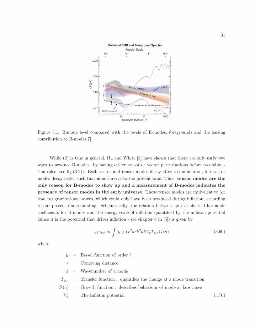
31
Figure 3.1: B-mode level compared with the levels of E-modes, foregrounds and the lensing
contribution to B-modes[7]
While (2) is true in general, Hu and White [8] have shown that there are only only two
ways to produce B-modes: by having either tensor or vector perturbations before recombina-
tion (also, see fig.(3.2)). Both vector and tensor modes decay after recombination, but vector
modes decay faster such that none survive to the present time. Thus, tensor modes are the
only reason for B-modes to show up and a measurement of B-modes indicates the
presence of tensor modes in the early universe. These tensor modes are equivalent to (or
lead to) gravitational waves, which could only have been produced during inflation, according
to our present understanding. Schematically, the relation between spin-2 spherical harmonic
coefficients for B-modes and the energy scale of inflation quantified by the inflaton potential
(since it is the potential that drives inflation - see chapter 6 in [5]) is given by
±2aℓm ∝∫
jℓ (r) r2drk2dkVφTφ,aG (a) (3.69)
where
jℓ = Bessel function of order ℓ
r = Comoving distance
k = Wavenumber of a mode
Tφ,a = Transfer function : quantifies the change at a mode transition
G (a) = Growth function : describes behaviour of mode at late times
Vφ = The Inflaton potential (3.70)
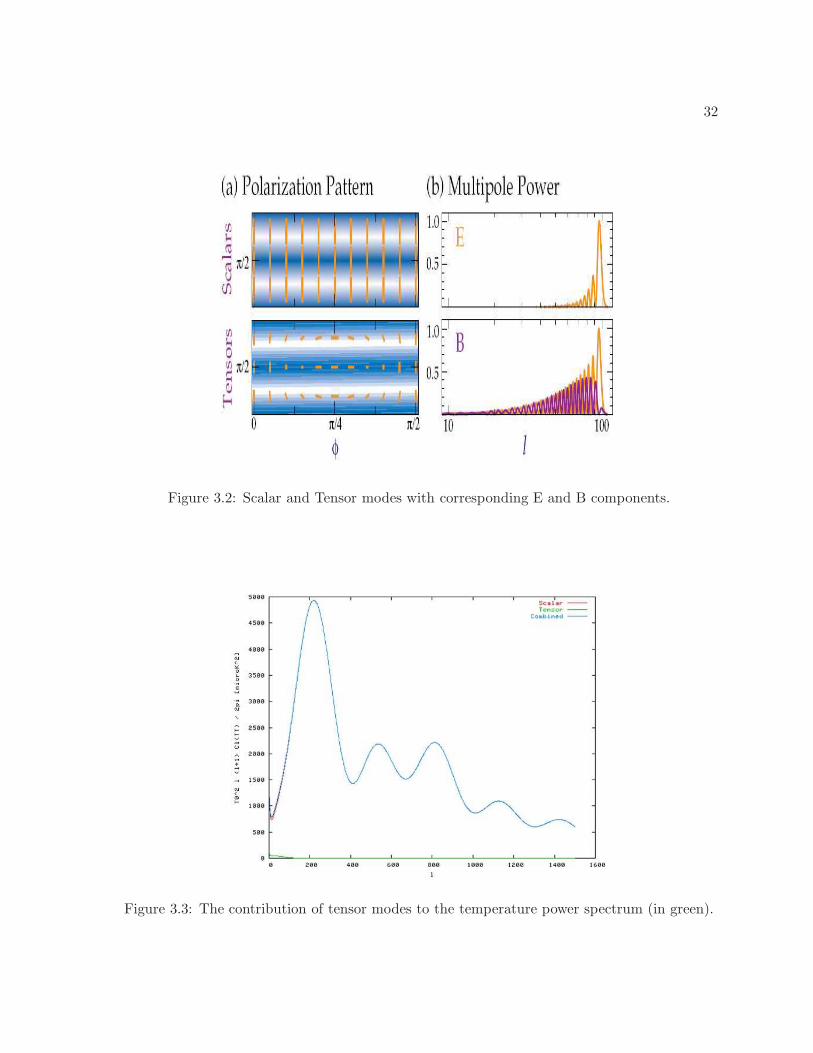
32
Figure 3.2: Scalar and Tensor modes with corresponding E and B components.
Figure 3.3: The contribution of tensor modes to the temperature power spectrum (in green).
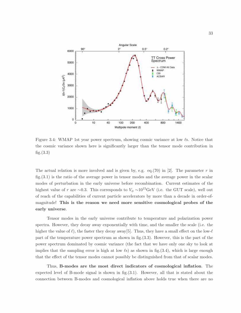
33
Figure 3.4: WMAP 1st year power spectrum, showing cosmic variance at low ℓs. Notice that
the cosmic variance shown here is significantly larger than the tensor mode contribution in
fig.(3.3)
The actual relation is more involved and is given by, e.g. eq.(70) in [2]. The parameter r in
fig.(3.1) is the ratio of the average power in tensor modes and the average power in the scalar
modes of perturbation in the early universe before recombination. Current estimates of the
highest value of r are ∼0.3. This corresponds to Vφ ∼1015GeV (i.e. the GUT scale), well out
of reach of the capabilities of current particle accelerators by more than a decade in order-of-
magnitude! This is the reason we need more sensitive cosmological probes of the
early universe.
Tensor modes in the early universe contribute to temperature and polarization power
spectra. However, they decay away exponentially with time, and the smaller the scale (i.e. the
higher the value of ℓ), the faster they decay away[5]. Thus, they have a small effect on the low-ℓ
part of the temperature power spectrum as shown in fig.(3.3). However, this is the part of the
power spectrum dominated by cosmic variance (the fact that we have only one sky to look at
implies that the sampling error is high at low ℓs) as shown in fig.(3.4), which is large enough
that the effect of the tensor modes cannot possibly be distinguished from that of scalar modes.
Thus, B-modes are the most direct indicators of cosmological inflation. The
expected level of B-mode signal is shown in fig.(3.1). However, all that is stated about the
connection between B-modes and cosmological inflation above holds true when there are no
34
foregrounds. There are two ways foregrounds can produce a spurious B-mode signal:
1. Emission: All processes that produce polarization, e.g. synchrotron can produce polarized
foregrounds in the presence of inhomogeneous magnetic fields.
2. Conversion: Gravitational lensing of the CMB by galaxies and galaxy clusters produces
distortions because lensing depends on the 2-D surface density, which is necessarily non-
uniform for clusters. This produces a “torsion” effect ([5] chapter 11) which converts a
portion of E-modes to B-modes. Since B-modes are an order of magnitude smaller, even
a small percentage of conversion leads to a large spurious B-mode effect.
These systematics will challenge the next generation of CMB polarization experiments.
In the next two chapters, we discuss results from recent experiments and the reason we
prefer interferometry over imaging.
35
Bibliography
[1] K. Rohlfs and T. L. Wilson, Tools of Radio Astronomy, Tools of Radio Astronomy, XVI,
423 pp. 127 figs., 20 tabs.. Springer-Verlag Berlin Heidelberg New York. Also Astronomy
and Astrophysics Library, 1996.
[2] Y.-T. Lin and B. D. Wandelt, “A beginner′s guide to the theory of CMB temperature and
polarization power spectra in the line-of-sight formalism,” Astroparticle Physics, vol. 25,
pp. 151–166, Mar. 2006.
[3] M. Zaldarriaga, Fluctuations in the cosmic microwave background, Ph.D. thesis, MAS-
SACHUSETTS INSTITUTE OF TECHNOLOGY, 1998.
[4] N. Goldberg, ,” J. Math. Phys., vol. 8, pp. 2155+, 1966.
[5] S. Dodelson, Modern cosmology, Modern cosmology / Scott Dodelson. Amsterdam (Nether-
lands): Academic Press. ISBN 0-12-219141-2, 2003, XIII + 440 p., 2003.
[6] G. B. Rybicki and A. P. Lightman, Radiative processes in astrophysics, New York, Wiley-
Interscience, 1979. 393 p., 1979.
[7] J. Bock, S. Church, M. Devlin, G. Hinshaw, A. Lange, A. Lee, L. Page, B. Partridge,
J. Ruhl, M. Tegmark, P. Timbie, R. Weiss, B. Winstein, and M. Zaldarriaga, “Task Force
on Cosmic Microwave Background Research,” ArXiv Astrophysics e-prints, Apr. 2006.
[8] W. Hu and M. White, “A CMB polarization primer,” New Astronomy, vol. 2, pp. 323–344,
Oct. 1997.
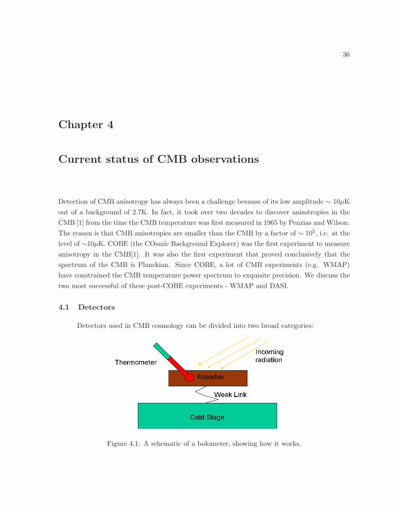
36
Chapter 4
Current status of CMB observations
Detection of CMB anisotropy has always been a challenge because of its low amplitude ∼ 10µK
out of a background of 2.7K. In fact, it took over two decades to discover anisotropies in the
CMB [1] from the time the CMB temperature was first measured in 1965 by Penzias and Wilson.
The reason is that CMB anisotropies are smaller than the CMB by a factor of ∼ 105, i.e. at the
level of ∼10µK. COBE (the COsmic Background Explorer) was the first experiment to measure
anisotropy in the CMB[1]. It was also the first experiment that proved conclusively that the
spectrum of the CMB is Planckian. Since COBE, a lot of CMB experiments (e.g. WMAP)
have constrained the CMB temperature power spectrum to exquisite precision. We discuss the
two most successful of these post-COBE experiments - WMAP and DASI.
4.1 Detectors
Detectors used in CMB cosmology can be divided into two broad categories:
Figure 4.1: A schematic of a bolometer, showing how it works.
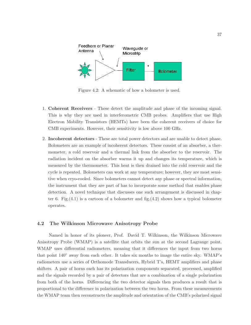
37
Figure 4.2: A schematic of how a bolometer is used.
1. Coherent Receivers - These detect the amplitude and phase of the incoming signal.
This is why they are used in interferometric CMB probes. Amplifiers that use High
Electron Mobility Transistors (HEMTs) have been the coherent receivers of choice for
CMB experiments. However, their sensitivity is low above 100 GHz.
2. Incoherent detectors - These are total power detectors and are unable to detect phase.
Bolometers are an example of incoherent detectors. These consist of an absorber, a ther-
mometer, a cold reservoir and a thermal link from the absorber to the reservoir. The
radiation incident on the absorber warms it up and changes its temperature, which is
measured by the thermometer. This heat is then drained into the cold reservoir and the
cycle is repeated. Bolometers can work at any temperature; however, they are most sensi-
tive when cryo-cooled. Since bolometers cannot detect any phase or spectral information,
the instrument that they are part of has to incorporate some method that enables phase
detection. A novel technique that discusses one such arrangement is discussed in chap-
ter 6. Fig.(4.1) is a cartoon of a bolometer and fig.(4.2) shows how a typical bolometer
operates.
4.2 The Wilkinson Microwave Anisotropy Probe
Named in honor of its pioneer, Prof. David T. Wilkinson, the Wilkinson Microwave
Anisotropy Probe (WMAP) is a satellite that orbits the sun at the second Lagrange point.
WMAP uses differential radiometers, meaning that it differences the input from two horns
that point 140 away from each other. It takes six months to image the entire sky. WMAP’s
radiometers use a series of Orthomode Transducers, Hybrid T’s, HEMT amplifiers and phase
shifters. A pair of horns each has its polarization components separated, processed, amplified
and the signals recorded by a pair of detectors that are a combination of a single polarization
from both of the horns. Differencing the two detector signals then produces a result that is
proportional to the difference in polarization between the two horns. From these measurements
the WMAP team then reconstructs the amplitude and orientation of the CMB’s polarized signal
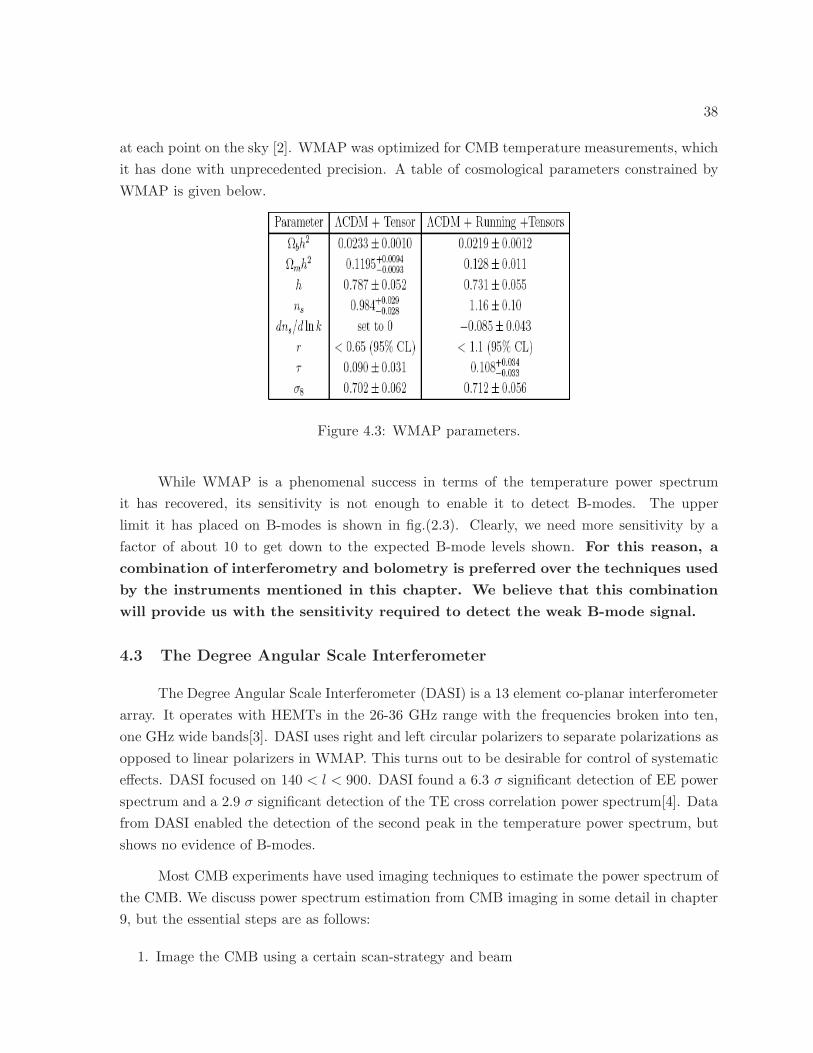
38
at each point on the sky [2]. WMAP was optimized for CMB temperature measurements, which
it has done with unprecedented precision. A table of cosmological parameters constrained by
WMAP is given below.
Figure 4.3: WMAP parameters.
While WMAP is a phenomenal success in terms of the temperature power spectrum
it has recovered, its sensitivity is not enough to enable it to detect B-modes. The upper
limit it has placed on B-modes is shown in fig.(2.3). Clearly, we need more sensitivity by a
factor of about 10 to get down to the expected B-mode levels shown. For this reason, a
combination of interferometry and bolometry is preferred over the techniques used
by the instruments mentioned in this chapter. We believe that this combination
will provide us with the sensitivity required to detect the weak B-mode signal.
4.3 The Degree Angular Scale Interferometer
The Degree Angular Scale Interferometer (DASI) is a 13 element co-planar interferometer
array. It operates with HEMTs in the 26-36 GHz range with the frequencies broken into ten,
one GHz wide bands[3]. DASI uses right and left circular polarizers to separate polarizations as
opposed to linear polarizers in WMAP. This turns out to be desirable for control of systematic
effects. DASI focused on 140 < l < 900. DASI found a 6.3 σ significant detection of EE power
spectrum and a 2.9 σ significant detection of the TE cross correlation power spectrum[4]. Data
from DASI enabled the detection of the second peak in the temperature power spectrum, but
shows no evidence of B-modes.
Most CMB experiments have used imaging techniques to estimate the power spectrum of
the CMB. We discuss power spectrum estimation from CMB imaging in some detail in chapter
9, but the essential steps are as follows:
1. Image the CMB using a certain scan-strategy and beam
39
2. Use a computationally optimal technique to extract the signal from the equation
d = A · s+ n (4.1)
where d is imaging data, A is a matrix that describes the beam and the scan strategy and
is called the “pointing matrix”, s the signal and n is the noise. This is where the image
is “pixelized”. Care has to be taken not to pixelize the data beyond the beam resolution.
3. Define likelihood. Using an optimal computational technique, estimate the values of Cℓs
that maximize the likelihood.
The trouble with imaging lies in points 2 and 3 above. In 2, we could decide to pixelize too
coarsely. This would certainly increase the signal-to-noise ratio, leading to lower errors in the
power spectrum, but the Cℓ estimates cannot be made for high ℓs. What is needed for future
CMB experiments is a system that can sample the power spectrum more directly and with
better control of systematics. The connection between an image and the power spectrum is
indorect; the power spectrum is the fourier transform of the two-point correlation function in
image space.
However, we show in chapter 5 that the power spectrum can also be expressed as a two-
point correlation function of the visibility (the output from one baseline of an interferometer).
This means that the interferometer samples ℓ-space directly - in fact, it turns out that every
unique baseline length corresponds to a unique ℓ-band where the width of the band depends
on the bandwidth of the instrument. Thus, there is never any confusion about the location of
the values of ℓ where the power spectrum is sampled - these are fixed in interferometry.
These and other characteristics of interferometry make its use preferable for CMB cos-
mology. The advantages of interferometry are discussed in detail in chapter 5. Additionally, in
chapter 6, we explore a new technique to utilize the information in a particular kind of inter-
ferometric system to enhance resolution in ℓ-space, leading to better estimates of Cℓs, as well
as better images.
40
Bibliography
[1] C. L. Bennett, A. J. Banday, K. M. Gorski, G. Hinshaw, P. Jackson, P. Keegstra, A. Kogut,
G. F. Smoot, D. T. Wilkinson, and E. L. Wright, “Four-Year COBE DMR Cosmic Mi-
crowave Background Observations: Maps and Basic Results,” ApJ Lett., vol. 464, pp. L1+,
June 1996.
[2] G. Hinshaw, M. R. Nolta, C. L. Bennett, R. Bean, O. Dore, M. R. Greason, M. Halpern, R. S.
Hill, N. Jarosik, A. Kogut, E. Komatsu, M. Limon, N. Odegard, S. S. Meyer, L. Page, H. V.
Peiris, D. N. Spergel, G. S. Tucker, L. Verde, J. L. Weiland, E. Wollack, and E. L. Wright,
“Three-Year Wilkinson Microwave Anisotropy Probe (WMAP) Observations: Temperature
Analysis,” ApJ Suppl., vol. 170, pp. 288–334, June 2007.
[3] N. W. Halverson, J. E. Carlstrom, M. Dragovan, W. L. Holzapfel, and J. Kovac, “DASI:
Degree Angular Scale Interferometer for imaging anisotropy in the cosmic microwave back-
ground,” in Proc. SPIE Vol. 3357, p. 416-423, Advanced Technology MMW, Radio, and
Terahertz Telescopes, Thomas G. Phillips; Ed., T. G. Phillips, Ed., July 1998, vol. 3357 of
Presented at the Society of Photo-Optical Instrumentation Engineers (SPIE) Conference,
pp. 416–423.
[4] E. M. Leitch, J. M. Kovac, N. W. Halverson, J. E. Carlstrom, C. Pryke, and M. W. E. Smith,
“Degree Angular Scale Interferometer 3 Year Cosmic Microwave Background Polarization
Results,” ApJ, vol. 624, pp. 10–20, May 2005.
41
Chapter 5
Interferometry
5.1 Overview
The observing wavelength of the Millimeter-wave Bolometric Interferometer (MBI)(∼3mm,
W-band) places it in the category of a radio telescope. However, MBI is not an imaging tele-
scope, but an interferometer. Even though it can be used as an imaging instrument (as shown
in the following chapter), we will discuss it here only as an interferometer.
Classically, interferometers were preferred over dish antennae for the following reason.
The angular resolution of a dish is given by θ ∼ λD . However, radio-waves are long-wavelength
and so for radio astronomy, we require huge single dishes for any reasonable angular resolution.
Interferometers are fundamentally different in that they produce diffraction patterns of the field-
of-view (‘FOV’ henceforth), and not images. Interferometers can achieve high angular resolution
by combining signals from widely separated small dishes. To a good first approximation, we can
treat them the way we treat diffraction slits. It will be shown later that there are fundamental
differences between a simple 1-slit diffraction of a point source and the diffraction of an extended
source through an interferometer.
5.2 The Mutual Coherence Function
While interferometry has many advantages (as described in §5.8), we need to be able to
relate the output of an interferometer to the image on the sky. It turns out that this connection
can be made via the study of coherence properties of the source. As will become clear later in
this chapter and the next, an interferometer makes use of both intensity and phase information,
so that this is not surprising. The following discussion on can be found in greater detail in several
texts, e.g. [1].
The simplest wave-field that can be imagined is the plane monochromatic wave. For
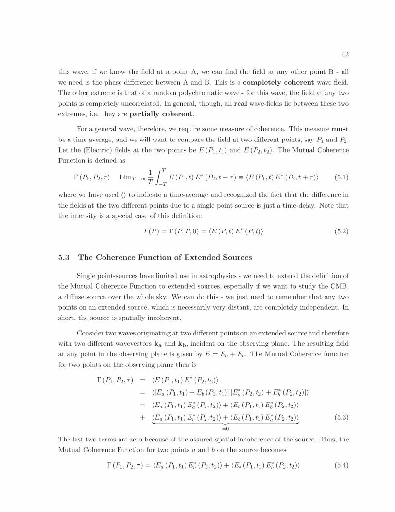
42
this wave, if we know the field at a point A, we can find the field at any other point B - all
we need is the phase-difference between A and B. This is a completely coherent wave-field.
The other extreme is that of a random polychromatic wave - for this wave, the field at any two
points is completely uncorrelated. In general, though, all real wave-fields lie between these two
extremes, i.e. they are partially coherent.
For a general wave, therefore, we require some measure of coherence. This measure must
be a time average, and we will want to compare the field at two different points, say P1 and P2.
Let the (Electric) fields at the two points be E (P1, t1) and E (P2, t2). The Mutual Coherence
Function is defined as
Γ (P1, P2, τ) = LimT→∞1
T
∫ T
−TE (P1, t)E
∗ (P2, t+ τ) ≡ 〈E (P1, t)E∗ (P2, t+ τ)〉 (5.1)
where we have used 〈〉 to indicate a time-average and recognized the fact that the difference in
the fields at the two different points due to a single point source is just a time-delay. Note that
the intensity is a special case of this definition:
I (P ) = Γ (P,P, 0) = 〈E (P, t)E∗ (P, t)〉 (5.2)
5.3 The Coherence Function of Extended Sources
Single point-sources have limited use in astrophysics - we need to extend the definition of
the Mutual Coherence Function to extended sources, especially if we want to study the CMB,
a diffuse source over the whole sky. We can do this - we just need to remember that any two
points on an extended source, which is necessarily very distant, are completely independent. In
short, the source is spatially incoherent.
Consider two waves originating at two different points on an extended source and therefore
with two different wavevectors ka and kb, incident on the observing plane. The resulting field
at any point in the observing plane is given by E = Ea + Eb. The Mutual Coherence function
for two points on the observing plane then is
Γ (P1, P2, τ) = 〈E (P1, t1)E∗ (P2, t2)〉
= 〈[Ea (P1, t1) + Eb (P1, t1)] [E∗a (P2, t2) + E∗
b (P2, t2)]〉= 〈Ea (P1, t1)E
∗a (P2, t2)〉+ 〈Eb (P1, t1)E
∗b (P2, t2)〉
+ 〈Ea (P1, t1)E∗b (P2, t2)〉+ 〈Eb (P1, t1)E
∗a (P2, t2)〉
︸ ︷︷ ︸
=0
(5.3)
The last two terms are zero because of the assured spatial incoherence of the source. Thus, the
Mutual Coherence Function for two points a and b on the source becomes
Γ (P1, P2, τ) = 〈Ea (P1, t1)E∗a (P2, t2)〉+ 〈Eb (P1, t1)E
∗b (P2, t2)〉 (5.4)
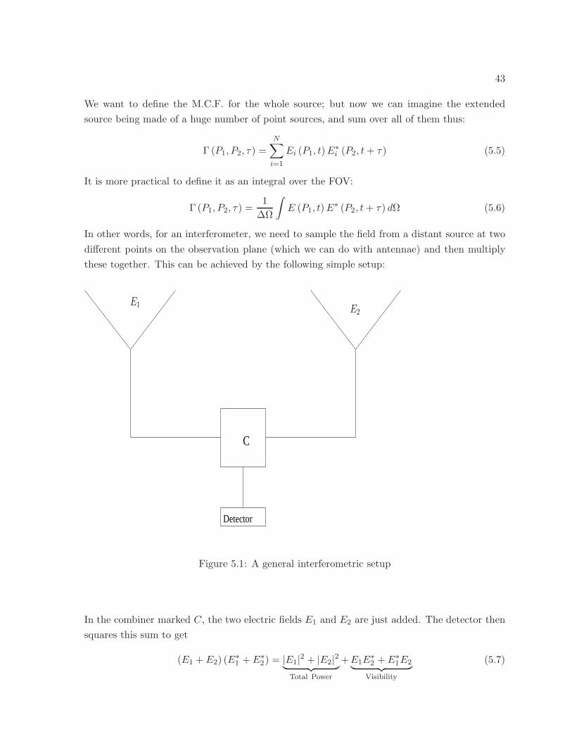
43
We want to define the M.C.F. for the whole source; but now we can imagine the extended
source being made of a huge number of point sources, and sum over all of them thus:
Γ (P1, P2, τ) =
N∑
i=1
Ei (P1, t)E∗i (P2, t+ τ) (5.5)
It is more practical to define it as an integral over the FOV:
Γ (P1, P2, τ) =1
∆Ω
∫
E (P1, t)E∗ (P2, t+ τ) dΩ (5.6)
In other words, for an interferometer, we need to sample the field from a distant source at two
different points on the observation plane (which we can do with antennae) and then multiply
these together. This can be achieved by the following simple setup:
C
Detector
E1E2
Figure 5.1: A general interferometric setup
In the combiner marked C, the two electric fields E1 and E2 are just added. The detector then
squares this sum to get
(E1 + E2) (E∗1 + E∗
2) = |E1|2 + |E2|2︸ ︷︷ ︸
Total Power
+E1E∗2 +E∗
1E2︸ ︷︷ ︸
Visibility
(5.7)
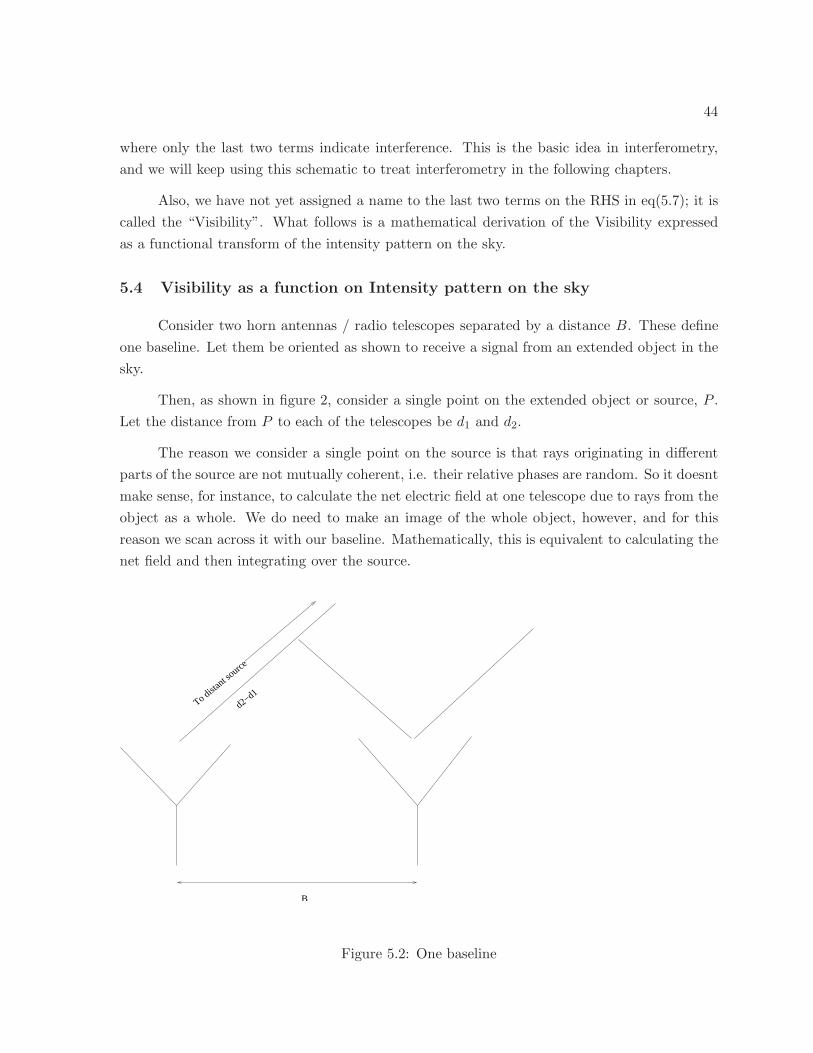
44
where only the last two terms indicate interference. This is the basic idea in interferometry,
and we will keep using this schematic to treat interferometry in the following chapters.
Also, we have not yet assigned a name to the last two terms on the RHS in eq(5.7); it is
called the “Visibility”. What follows is a mathematical derivation of the Visibility expressed
as a functional transform of the intensity pattern on the sky.
5.4 Visibility as a function on Intensity pattern on the sky
Consider two horn antennas / radio telescopes separated by a distance B. These define
one baseline. Let them be oriented as shown to receive a signal from an extended object in the
sky.
Then, as shown in figure 2, consider a single point on the extended object or source, P .
Let the distance from P to each of the telescopes be d1 and d2.
The reason we consider a single point on the source is that rays originating in different
parts of the source are not mutually coherent, i.e. their relative phases are random. So it doesnt
make sense, for instance, to calculate the net electric field at one telescope due to rays from the
object as a whole. We do need to make an image of the whole object, however, and for this
reason we scan across it with our baseline. Mathematically, this is equivalent to calculating the
net field and then integrating over the source.
To distant s
ource
d2−d1
B
Figure 5.2: One baseline
45
Let (x, y) be the co-ordinate system on the source. Let I (x, y) be the intensity as a
function of position on the source, and let E (x, y) be the electric field due to the source on
both the antennas. D is the distance between the telescopes and the source.
There is a time delay of (d2−d1)c between the signals received by the two telescopes (see
fig.(5.2)). The electric fields at the two telescopes can be written as:
E1 = E (x, y) eiω
“
t− d1c
”
(5.8)
E2 = E (x, y) eiω
“
t− d2c
”
(5.9)
Consider now the product of these two electric fields. In brief, it is only by multiplying
the two signals that we can get interference, as discussed in §5.3.
E1E∗2 ∼ E2 (x, y) e
iω“
t− d1c−td2
c+
”
= I (x, y) eiωc(d2−d1) (5.10)
Looking at figure 3, the two distances d1 and d2 can be written as
d21 =
(
x− 1
2B
)2
+ y2 +D2 = D2
1 +y2
D2+
(
x− 12B
D
)2
(5.11)
d22 =
(
x+1
2B
)2
+ y2 +D2 = D2
1 +y2
D2+
(
x+ 12B
D
)2
(5.12)
Clearly, BD ≪ 1; in other words, the distance between us and the source is much greater
than the length of the baseline. We assume that xD ,
yD ≪ 1, or that the size of the source is
much smaller than the distance between us and the source.
Then,
d1 ≃ D[
1 +1
2
y2
D2+
1
2
(
x− 12B
D
)]
(5.13)
d2 ≃ D[
1 +1
2
y2
D2+
1
2
(
x+ 12B
D
)]
(5.14)
so that
d2 − d1 = D.1
2.
1
D2. 2. 2.
1
2. Bx =
Bx
D(5.15)
46
⇒ E1E∗2 ∼ I (x, y) ei
ωc
BxD = I (x, y) ei2π
BxDλ (5.16)
All this is fine, but we would like to work in terms of angles, so we change variables to α = xD ,
β = yD so that
E1E∗2 ∼ I (α, β) ei2π
Bλα (5.17)
However, the basis (α, β) is relative to the source, and not the observation plane or the sky. We
therefore slip the formalism into something more comfortable and convenient - the equitorial
co-ordinates, thus:
α = cos θx′ + sin θy′ (5.18)
β = sin θx′ + cos θy′ (5.19)
Then,
E1E∗2 ∼ I
(x′, y′
)ei2π
Bλ
(cos θx′+sin θy′) (5.20)
Write
u =B
λcos θ (5.21)
v =B
λsin θ (5.22)
These are what are called the u, v co-ordinates. Now we integrate over x′ and y′ to get:∫ ∫
E1E∗2dx
′dy′ = K
∫ ∫
I(x′, y′
)ei2π(ux′+vy′)dx′dy′ (5.23)
But the right side of the equation is just the fourier transform of I (x′, y′). The left hand side
is what we call visibility.
In this discussion, we ignored the effect of the diffraction patterns of the telescopes /
antennas themselves. We can introduce it in equations 1 and 2 above:
E1 =√
A (x, y)E (x, y) eiω
“
t− d1c
”
(5.24)
E2 =√
A (x, y)E (x, y) eiω
“
t− d2c
”
(5.25)
and then follow it through, to get:∫ ∫
E1E∗2dx
′dy′ = K
∫ ∫
A(x′, y′
)I(x′, y′
)ei2π(ux′+vy′)dx′dy′ (5.26)
We do not need to make the small-sky patch approximation to get a useful result, though.
It just so happens that in this approximation, the output of the interferometer, the “Visibility”,
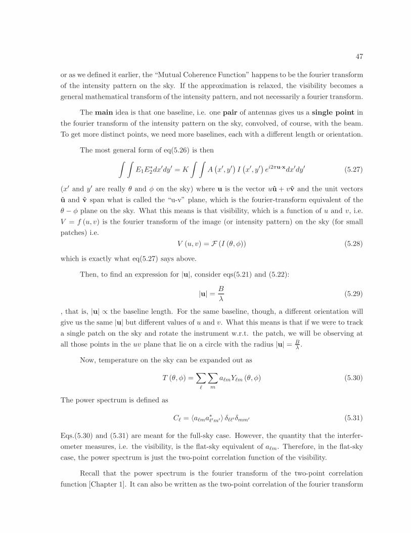
47
or as we defined it earlier, the “Mutual Coherence Function” happens to be the fourier transform
of the intensity pattern on the sky. If the approximation is relaxed, the visibility becomes a
general mathematical transform of the intensity pattern, and not necessarily a fourier transform.
The main idea is that one baseline, i.e. one pair of antennas gives us a single point in
the fourier transform of the intensity pattern on the sky, convolved, of course, with the beam.
To get more distinct points, we need more baselines, each with a different length or orientation.
The most general form of eq(5.26) is then
∫ ∫
E1E∗2dx
′dy′ = K
∫ ∫
A(x′, y′
)I(x′, y′
)ei2πu·xdx′dy′ (5.27)
(x′ and y′ are really θ and φ on the sky) where u is the vector uu + vv and the unit vectors
u and v span what is called the “u-v” plane, which is the fourier-transform equivalent of the
θ − φ plane on the sky. What this means is that visibility, which is a function of u and v, i.e.
V = f (u, v) is the fourier transform of the image (or intensity pattern) on the sky (for small
patches) i.e.
V (u, v) = F (I (θ, φ)) (5.28)
which is exactly what eq(5.27) says above.
Then, to find an expression for |u|, consider eqs(5.21) and (5.22):
|u| = B
λ(5.29)
, that is, |u| ∝ the baseline length. For the same baseline, though, a different orientation will
give us the same |u| but different values of u and v. What this means is that if we were to track
a single patch on the sky and rotate the instrument w.r.t. the patch, we will be observing at
all those points in the uv plane that lie on a circle with the radius |u| = Bλ .
Now, temperature on the sky can be expanded out as
T (θ, φ) =∑
ℓ
∑
m
aℓmYℓm (θ, φ) (5.30)
The power spectrum is defined as
Cℓ = 〈aℓma∗ℓ′m′〉 δℓℓ′δmm′ (5.31)
Eqs.(5.30) and (5.31) are meant for the full-sky case. However, the quantity that the interfer-
ometer measures, i.e. the visibility, is the flat-sky equivalent of aℓm. Therefore, in the flat-sky
case, the power spectrum is just the two-point correlation function of the visibility.
Recall that the power spectrum is the fourier transform of the two-point correlation
function [Chapter 1]. It can also be written as the two-point correlation of the fourier transform
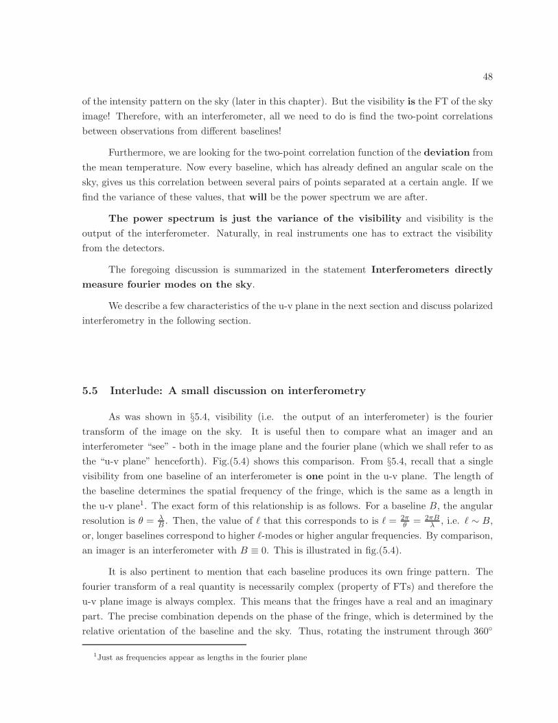
48
of the intensity pattern on the sky (later in this chapter). But the visibility is the FT of the sky
image! Therefore, with an interferometer, all we need to do is find the two-point correlations
between observations from different baselines!
Furthermore, we are looking for the two-point correlation function of the deviation from
the mean temperature. Now every baseline, which has already defined an angular scale on the
sky, gives us this correlation between several pairs of points separated at a certain angle. If we
find the variance of these values, that will be the power spectrum we are after.
The power spectrum is just the variance of the visibility and visibility is the
output of the interferometer. Naturally, in real instruments one has to extract the visibility
from the detectors.
The foregoing discussion is summarized in the statement Interferometers directly
measure fourier modes on the sky.
We describe a few characteristics of the u-v plane in the next section and discuss polarized
interferometry in the following section.
5.5 Interlude: A small discussion on interferometry
As was shown in §5.4, visibility (i.e. the output of an interferometer) is the fourier
transform of the image on the sky. It is useful then to compare what an imager and an
interferometer “see” - both in the image plane and the fourier plane (which we shall refer to as
the “u-v plane” henceforth). Fig.(5.4) shows this comparison. From §5.4, recall that a single
visibility from one baseline of an interferometer is one point in the u-v plane. The length of
the baseline determines the spatial frequency of the fringe, which is the same as a length in
the u-v plane1. The exact form of this relationship is as follows. For a baseline B, the angular
resolution is θ = λB . Then, the value of ℓ that this corresponds to is ℓ = 2π
θ = 2πBλ , i.e. ℓ ∼ B,
or, longer baselines correspond to higher ℓ-modes or higher angular frequencies. By comparison,
an imager is an interferometer with B ≡ 0. This is illustrated in fig.(5.4).
It is also pertinent to mention that each baseline produces its own fringe pattern. The
fourier transform of a real quantity is necessarily complex (property of FTs) and therefore the
u-v plane image is always complex. This means that the fringes have a real and an imaginary
part. The precise combination depends on the phase of the fringe, which is determined by the
relative orientation of the baseline and the sky. Thus, rotating the instrument through 360
1Just as frequencies appear as lengths in the fourier plane
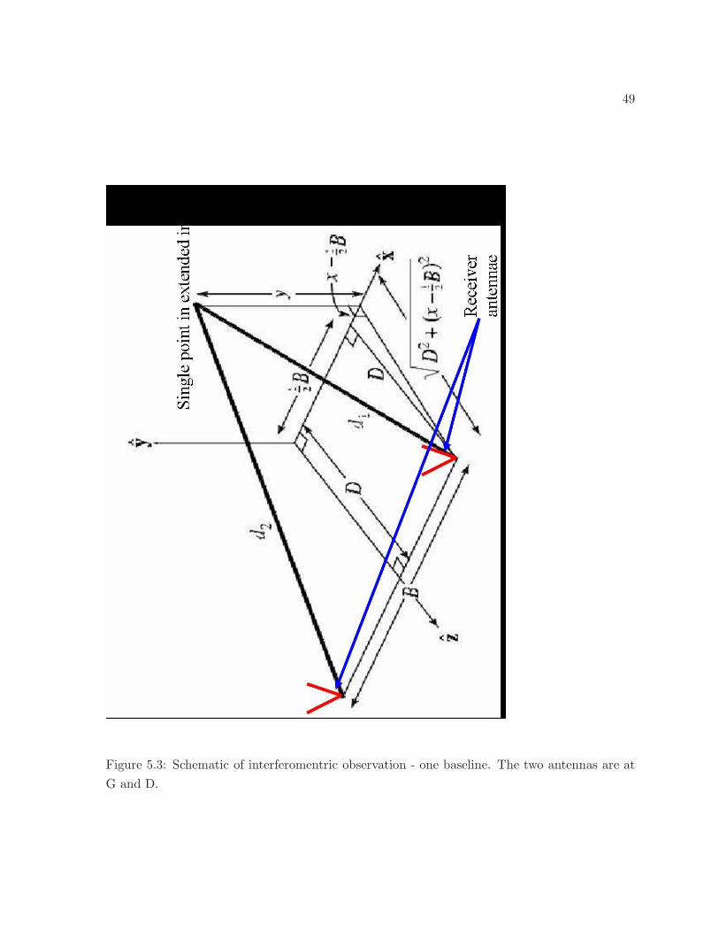
49
Figure 5.3: Schematic of interferomentric observation - one baseline. The two antennas are at
G and D.
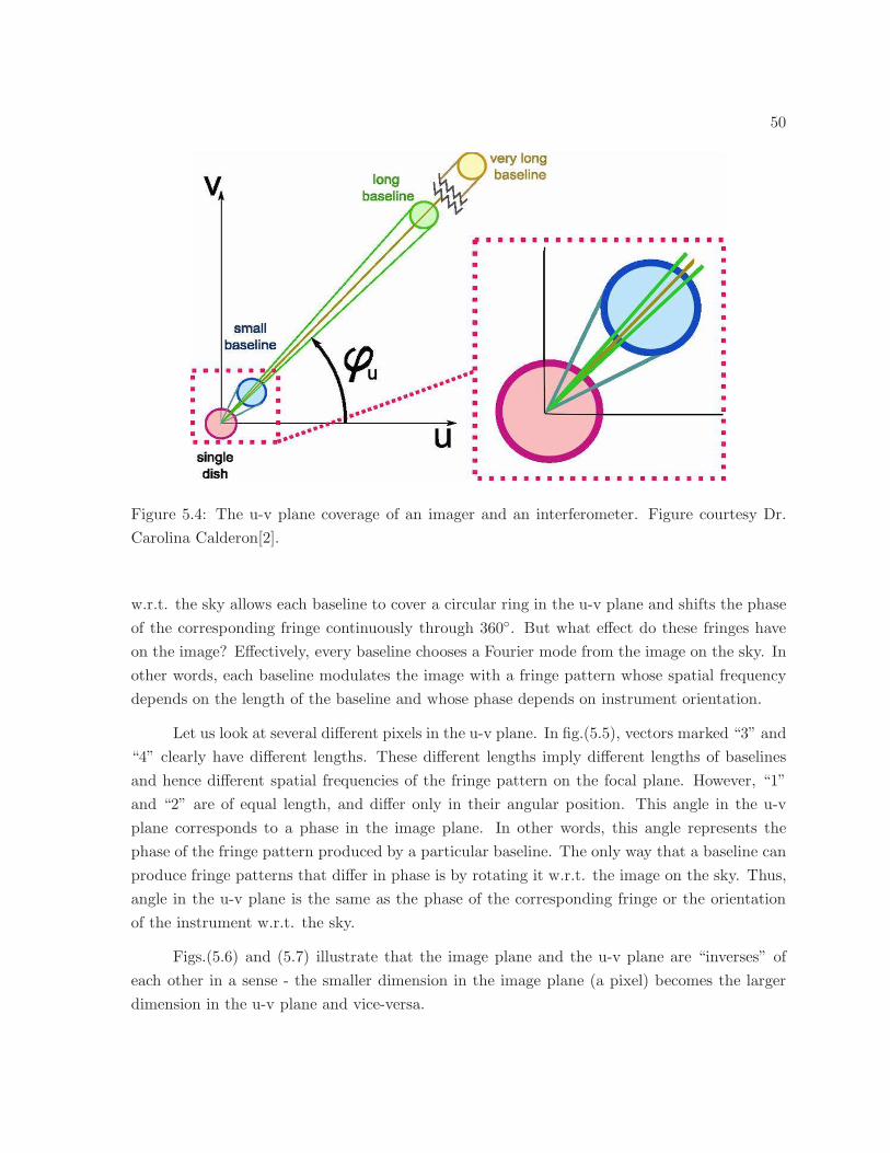
50
Figure 5.4: The u-v plane coverage of an imager and an interferometer. Figure courtesy Dr.
Carolina Calderon[2].
w.r.t. the sky allows each baseline to cover a circular ring in the u-v plane and shifts the phase
of the corresponding fringe continuously through 360. But what effect do these fringes have
on the image? Effectively, every baseline chooses a Fourier mode from the image on the sky. In
other words, each baseline modulates the image with a fringe pattern whose spatial frequency
depends on the length of the baseline and whose phase depends on instrument orientation.
Let us look at several different pixels in the u-v plane. In fig.(5.5), vectors marked “3” and
“4” clearly have different lengths. These different lengths imply different lengths of baselines
and hence different spatial frequencies of the fringe pattern on the focal plane. However, “1”
and “2” are of equal length, and differ only in their angular position. This angle in the u-v
plane corresponds to a phase in the image plane. In other words, this angle represents the
phase of the fringe pattern produced by a particular baseline. The only way that a baseline can
produce fringe patterns that differ in phase is by rotating it w.r.t. the image on the sky. Thus,
angle in the u-v plane is the same as the phase of the corresponding fringe or the orientation
of the instrument w.r.t. the sky.
Figs.(5.6) and (5.7) illustrate that the image plane and the u-v plane are “inverses” of
each other in a sense - the smaller dimension in the image plane (a pixel) becomes the larger
dimension in the u-v plane and vice-versa.
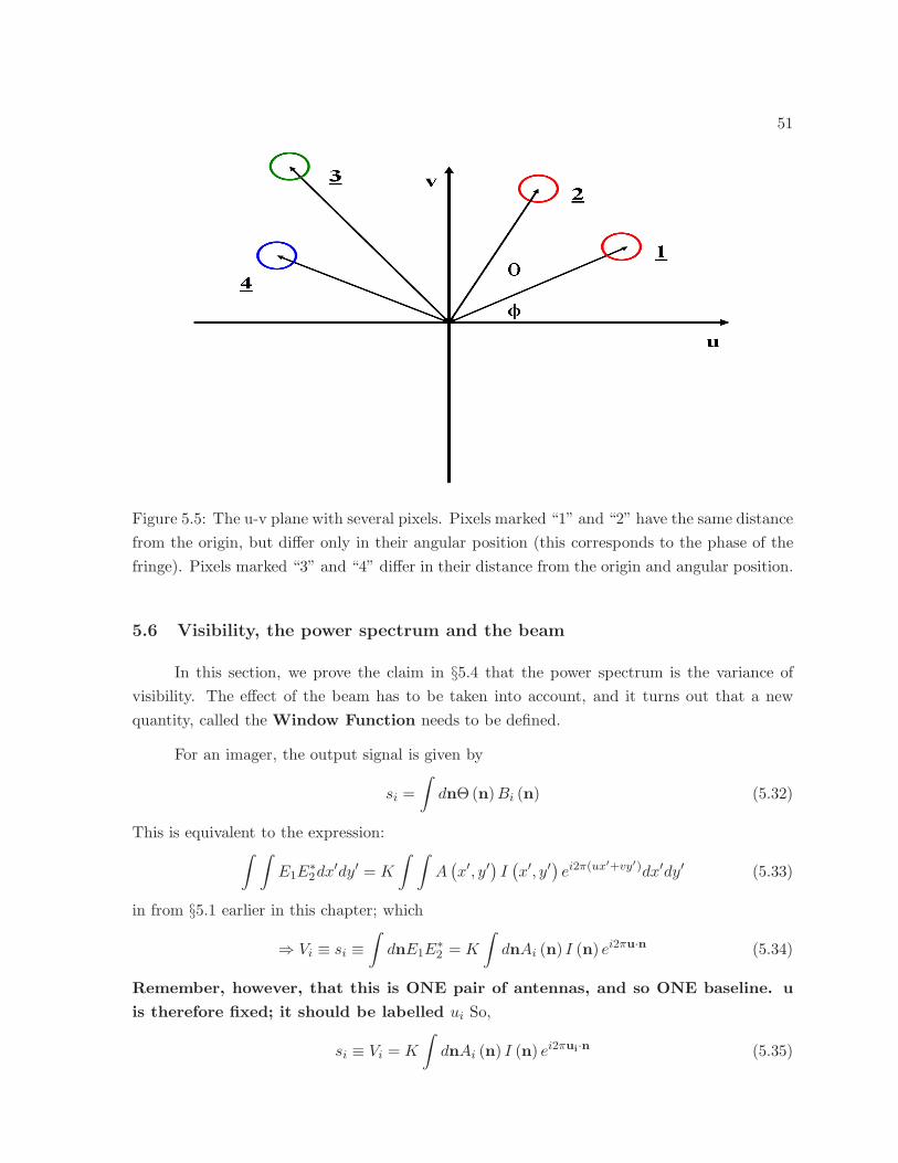
51
Figure 5.5: The u-v plane with several pixels. Pixels marked “1” and “2” have the same distance
from the origin, but differ only in their angular position (this corresponds to the phase of the
fringe). Pixels marked “3” and “4” differ in their distance from the origin and angular position.
5.6 Visibility, the power spectrum and the beam
In this section, we prove the claim in §5.4 that the power spectrum is the variance of
visibility. The effect of the beam has to be taken into account, and it turns out that a new
quantity, called the Window Function needs to be defined.
For an imager, the output signal is given by
si =
∫
dnΘ (n)Bi (n) (5.32)
This is equivalent to the expression:∫ ∫
E1E∗2dx
′dy′ = K
∫ ∫
A(x′, y′
)I(x′, y′
)ei2π(ux′+vy′)dx′dy′ (5.33)
in from §5.1 earlier in this chapter; which
⇒ Vi ≡ si ≡∫
dnE1E∗2 = K
∫
dnAi (n) I (n) ei2πu·n (5.34)
Remember, however, that this is ONE pair of antennas, and so ONE baseline. u
is therefore fixed; it should be labelled ui So,
si ≡ Vi = K
∫
dnAi (n) I (n) ei2πui·n (5.35)
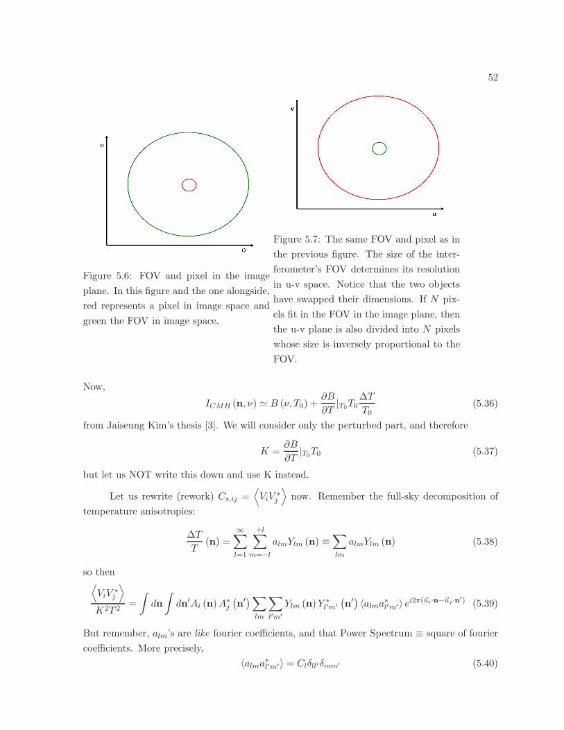
52
Figure 5.6: FOV and pixel in the image
plane. In this figure and the one alongside,
red represents a pixel in image space and
green the FOV in image space.
Figure 5.7: The same FOV and pixel as in
the previous figure. The size of the inter-
ferometer’s FOV determines its resolution
in u-v space. Notice that the two objects
have swapped their dimensions. If N pix-
els fit in the FOV in the image plane, then
the u-v plane is also divided into N pixels
whose size is inversely proportional to the
FOV.
Now,
ICMB (n, ν) ≃ B (ν, T0) +∂B
∂T|T0T0
∆T
T0(5.36)
from Jaiseung Kim’s thesis [3]. We will consider only the perturbed part, and therefore
K =∂B
∂T|T0T0 (5.37)
but let us NOT write this down and use K instead.
Let us rewrite (rework) Cs,ij =⟨
ViV∗j
⟩
now. Remember the full-sky decomposition of
temperature anisotropies:
∆T
T(n) =
∞∑
l=1
+l∑
m=−lalmYlm (n) ≡
∑
lm
almYlm (n) (5.38)
so then⟨
ViV∗j
⟩
K2T 2=
∫
dn
∫
dn′Ai (n)A∗j
(n′)∑
lm
∑
l′m′
Ylm (n)Y ∗l′m′
(n′) 〈alma∗l′m′〉 ei2π(~ui·n−~uj ·n′) (5.39)
But remember, alm’s are like fourier coefficients, and that Power Spectrum ≡ square of fourier
coefficients. More precisely,
〈alma∗l′m′〉 = Clδll′δmm′ (5.40)
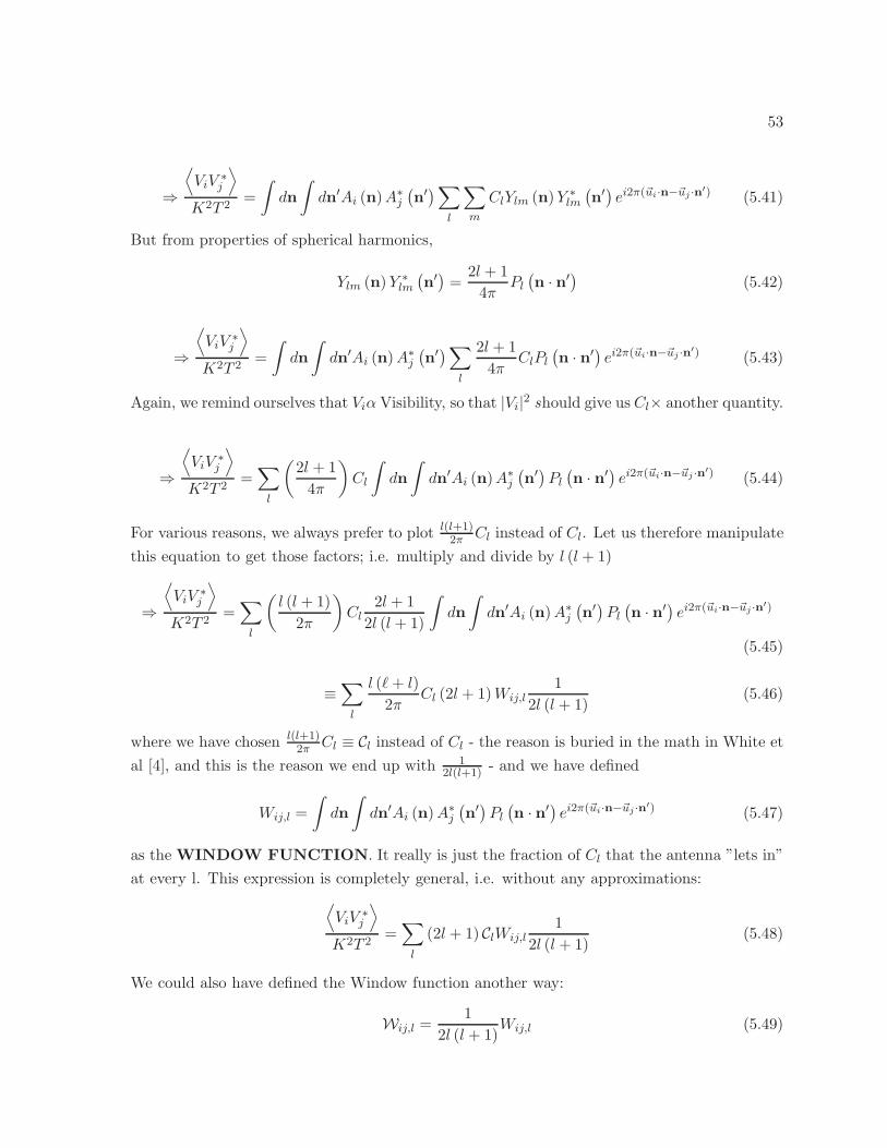
53
⇒
⟨
ViV∗j
⟩
K2T 2=
∫
dn
∫
dn′Ai (n)A∗j
(n′)∑
l
∑
m
ClYlm (n)Y ∗lm
(n′) ei2π(~ui·n−~uj ·n′) (5.41)
But from properties of spherical harmonics,
Ylm (n)Y ∗lm
(n′) =
2l + 1
4πPl(n · n′) (5.42)
⇒
⟨
ViV∗j
⟩
K2T 2=
∫
dn
∫
dn′Ai (n)A∗j
(n′)∑
l
2l + 1
4πClPl
(n · n′) ei2π(~ui·n−~uj ·n′) (5.43)
Again, we remind ourselves that Viα Visibility, so that |Vi|2 should give us Cl× another quantity.
⇒
⟨
ViV∗j
⟩
K2T 2=∑
l
(2l + 1
4π
)
Cl
∫
dn
∫
dn′Ai (n)A∗j
(n′)Pl
(n · n′) ei2π(~ui·n−~uj ·n′) (5.44)
For various reasons, we always prefer to plot l(l+1)2π Cl instead of Cl. Let us therefore manipulate
this equation to get those factors; i.e. multiply and divide by l (l + 1)
⇒
⟨
ViV∗j
⟩
K2T 2=∑
l
(l (l + 1)
2π
)
Cl2l + 1
2l (l + 1)
∫
dn
∫
dn′Ai (n)A∗j
(n′)Pl
(n · n′) ei2π(~ui·n−~uj ·n′)
(5.45)
≡∑
l
l (ℓ+ l)
2πCl (2l + 1)Wij,l
1
2l (l + 1)(5.46)
where we have chosen l(l+1)2π Cl ≡ Cl instead of Cl - the reason is buried in the math in White et
al [4], and this is the reason we end up with 12l(l+1) - and we have defined
Wij,l =
∫
dn
∫
dn′Ai (n)A∗j
(n′)Pl
(n · n′) ei2π(~ui·n−~uj ·n′) (5.47)
as the WINDOW FUNCTION. It really is just the fraction of Cl that the antenna ”lets in”
at every l. This expression is completely general, i.e. without any approximations:
⟨
ViV∗j
⟩
K2T 2=∑
l
(2l + 1) ClWij,l1
2l (l + 1)(5.48)
We could also have defined the Window function another way:
Wij,l =1
2l (l + 1)Wij,l (5.49)
54
where Wij,l is now the ‘net’ Window function, and we have⟨
ViV∗j
⟩
K2T 2=∑
l
(2l + 1) ClWij,l (5.50)
Aside: this implies that the height of the ‘net’ window function decreases with increasing
l. Physically, what this means is that by increasing the baseline, the amount of light we let
into the telescope system decreases compared to the amount that would have been let in had
the telescope been a filled aperture with the length of baseline as the diameter. Succinctly, the
‘filling-factor’ (the ratio of the total area of antennas in one baseline to the area of a dish with
the baseline as a diameter) decreses with increasing l (equivalent to increasing the baseline).
The foregoing argument implies thatWij,l ∼ l−2, which is indeed the case, as can be seen
in the above expression.
In the following, we will derive an expression for Wij,l, and will finally write down the
expression for Wij,l at the end of this section.
We can now apply the FLAT-SKY APPROXIMATION (small θ, large l):
1. x and x′ are vectors in directions n n′ respectively. Approximating them to 2-D vectors
on the sky ⇒Pl(n · n′) ≃ Pl
(cos|x− x′|
)(5.51)
and ∫
dn
∫
dn′ ≃∫
d2x
∫
d2x′ (5.52)
⇒Wij,l =
∫
d2x
∫
d2x′Ai (x)A∗j
(x′)Pl
(cos|x− x′|
)ei2π(~ui·x−~uj ·x′) (5.53)
This is the modified version of eq. 11.40 in Dodelson.
2.
Pl(cos|x− x′|
)→ J0
(l|x− x′|
)≡ 1
2π
∫ 2π
0dφe−il|x−x′| cosφ (5.54)
where the last equality is the definition of the Bessel function of order l.
Now, l|x − x′| cosφ can be written as l · (x− x′), because φ is really just a parameter
we are integrating over. We are therefore free to provide our own physical interpretation of it.
The one convenient for us is: φ is an angle in l-space, and is defined as φ = tan−1 lylx
and then
l =√
l2x + l2y.
So then
⇒ Wij,l =1
2π
∫
d2x
∫
d2x′Ai (x)A∗j
(x′) 1
2π
∫ 2π
0dφe−il·(x−x′)ei2π(~ui·x−~uj ·x′) (5.55)
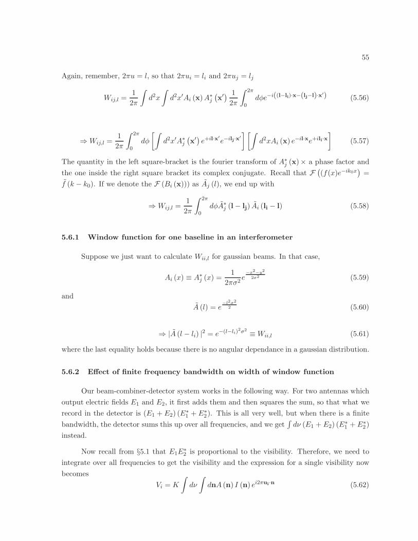
55
Again, remember, 2πu = l, so that 2πui = li and 2πuj = lj
Wij,l =1
2π
∫
d2x
∫
d2x′Ai (x)A∗j
(x′) 1
2π
∫ 2π
0dφe−i((l−li)·x−(lj−l)·x′) (5.56)
⇒Wij,l =1
2π
∫ 2π
0dφ
[∫
d2x′A∗j
(x′) e+il·x
′
e−ilj·x′
] [∫
d2xAi (x) e−il·xe+ili·x]
(5.57)
The quantity in the left square-bracket is the fourier transform of A∗j (x)× a phase factor and
the one inside the right square bracket its complex conjugate. Recall that F((f(x)e−ik0x
)=
f (k − k0). If we denote the F (Bi (x))) as Aj (l), we end up with
⇒Wij,l =1
2π
∫ 2π
0dφA∗
j (l− lj) Ai (li − l) (5.58)
5.6.1 Window function for one baseline in an interferometer
Suppose we just want to calculate Wii,l for gaussian beams. In that case,
Ai (x) ≡ A∗j (x) =
1
2πσ2e
−x2−y2
2σ2 (5.59)
and
A (l) = e−l2σ2
2 (5.60)
⇒ |A (l − li) |2 = e−(l−li)2σ2 ≡Wii,l (5.61)
where the last equality holds because there is no angular dependance in a gaussian distribution.
5.6.2 Effect of finite frequency bandwidth on width of window function
Our beam-combiner-detector system works in the following way. For two antennas which
output electric fields E1 and E2, it first adds them and then squares the sum, so that what we
record in the detector is (E1 + E2) (E∗1 + E∗
2). This is all very well, but when there is a finite
bandwidth, the detector sums this up over all frequencies, and we get∫dν (E1 + E2) (E∗
1 + E∗2)
instead.
Now recall from §5.1 that E1E∗2 is proportional to the visibility. Therefore, we need to
integrate over all frequencies to get the visibility and the expression for a single visibility now
becomes
Vi = K
∫
dν
∫
dnA (n) I (n) ei2πui·n (5.62)
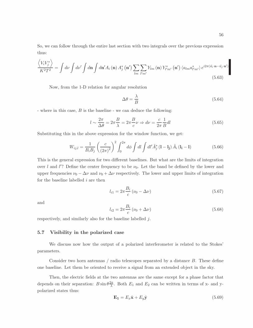
56
So, we can follow through the entire last section with two integrals over the previous expression
thus:⟨
ViV∗j
⟩
K2T 2=
∫
dν
∫
dν ′∫
dn
∫
dn′Ai (n)A∗j
(n′)∑
lm
∑
l′m′
Ylm (n)Y ∗l′m′
(n′) 〈alma∗l′m′〉 ei2π(~ui·n−~uj ·n′)
(5.63)
Now, from the 1-D relation for angular resolution
∆θ =λ
B(5.64)
- where in this case, B is the baseline - we can deduce the following:
l ∼ 2π
∆θ= 2π
B
λ= 2π
B
cν ⇒ dν =
c
2π
1
Bdl (5.65)
Substituting this in the above expression for the window function, we get:
Wij,l =1
BiBj
(c
(2π)2
)2 ∫ 2π
0dφ
∫
dl
∫
dl′A∗j (l− lj) Ai (li − l) (5.66)
This is the general expression for two different baselines. But what are the limits of integration
over l and l′? Define the center frequency to be ν0. Let the band be defined by the lower and
upper frequencies ν0−∆ν and ν0 + ∆ν respectively. The lower and upper limits of integration
for the baseline labelled i are then
li1 = 2πBic
(ν0 −∆ν) (5.67)
and
li2 = 2πBic
(ν0 + ∆ν) (5.68)
respectively, and similarly also for the baseline labelled j.
5.7 Visibility in the polarized case
We discuss now how the output of a polarized interferometer is related to the Stokes’
parameters.
Consider two horn antennas / radio telescopes separated by a distance B. These define
one baseline. Let them be oriented to receive a signal from an extended object in the sky.
Then, the electric fields at the two antennas are the same except for a phase factor that
depends on their separation: B sin θ 2πλ . Both E1 and E2 can be written in terms of x- and y-
polarized states thus:
E1 = Exx +Eyy (5.69)
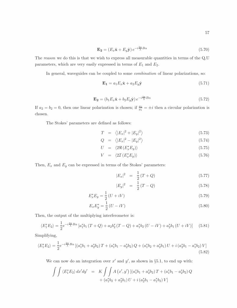
57
E2 = (Exx + Eyy) e−i2πλBα (5.70)
The reason we do this is that we wish to express all measurable quantities in terms of the Q,U
parameters, which are very easily expressed in terms of E1 and E2.
In general, waveguides can be coupled to some combination of linear polarizations, so:
E1 = a1Exx + a2Eyy (5.71)
E2 = (b1Exx + b2Eyy) e−i2πλBα (5.72)
If a2 = b2 = 0, then one linear polarization is chosen; if a2a1
= ±i then a circular polarization is
chosen.
The Stokes’ parameters are defined as follows:
T =⟨|Ex|2 + |Ey|2
⟩(5.73)
Q =⟨|Ex|2 − |Ey|2
⟩(5.74)
U = 〈2ℜ (E∗xEy)〉 (5.75)
V = 〈2I (E∗xEy)〉 (5.76)
Then, Ex and Ey can be expressed in terms of the Stokes’ parameters:
|Ex|2 =1
2(T +Q) (5.77)
|Ey|2 =1
2(T −Q) (5.78)
E∗xEy =
1
2(U + iV ) (5.79)
ExE∗y =
1
2(U − iV ) (5.80)
Then, the output of the multiplying interferometer is:
〈E∗1E2〉 =
1
2e−i
2πλBα [a∗1b1 (T +Q) + a2b
∗2 (T −Q) + a∗1b2 (U − iV ) + a∗2b1 (U + iV )] (5.81)
Simplifying,
〈E∗1E2〉 =
1
2e−i
2πλBα [(a∗1b1 + a∗2b2)T + (a∗1b1 − a∗2b2)Q+ (a∗1b2 + a∗2b1)U + i (a∗2b1 − a∗1b2)V ]
(5.82)
We can now do an integration over x′ and y′, as shown in §5.1, to end up with:∫ ∫
〈E∗1E2〉 dx′dy′ = K
∫ ∫
A(x′, y′
)[(a∗1b1 + a∗2b2)T + (a∗1b1 − a∗2b2)Q
+ (a∗1b2 + a∗2b1)U + i (a∗2b1 − a∗1b2)V ]
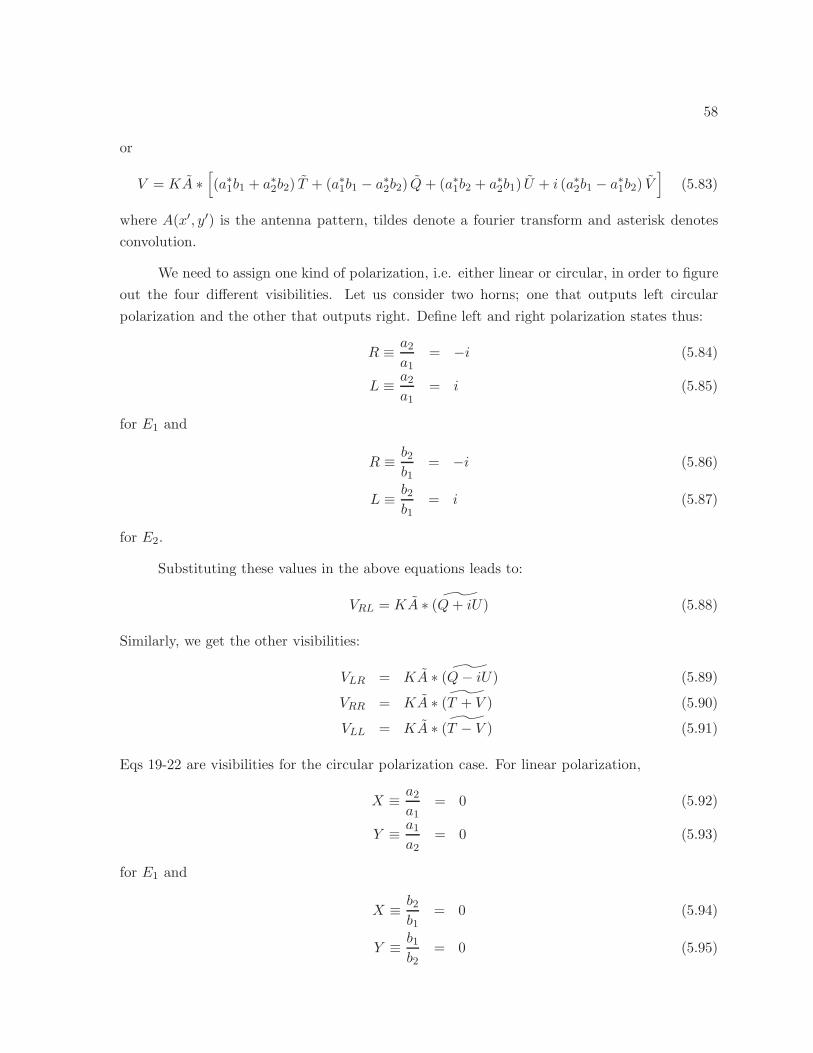
58
or
V = KA ∗[
(a∗1b1 + a∗2b2) T + (a∗1b1 − a∗2b2) Q+ (a∗1b2 + a∗2b1) U + i (a∗2b1 − a∗1b2) V]
(5.83)
where A(x′, y′) is the antenna pattern, tildes denote a fourier transform and asterisk denotes
convolution.
We need to assign one kind of polarization, i.e. either linear or circular, in order to figure
out the four different visibilities. Let us consider two horns; one that outputs left circular
polarization and the other that outputs right. Define left and right polarization states thus:
R ≡ a2
a1= −i (5.84)
L ≡ a2
a1= i (5.85)
for E1 and
R ≡ b2b1
= −i (5.86)
L ≡ b2b1
= i (5.87)
for E2.
Substituting these values in the above equations leads to:
VRL = KA ∗ ˜(Q+ iU) (5.88)
Similarly, we get the other visibilities:
VLR = KA ∗ ˜(Q− iU) (5.89)
VRR = KA ∗ ˜(T + V ) (5.90)
VLL = KA ∗ ˜(T − V ) (5.91)
Eqs 19-22 are visibilities for the circular polarization case. For linear polarization,
X ≡ a2
a1= 0 (5.92)
Y ≡ a1
a2= 0 (5.93)
for E1 and
X ≡ b2b1
= 0 (5.94)
Y ≡ b1b2
= 0 (5.95)
59
for E2 and so
VXY = KA ∗ ˜(U + iV ) (5.96)
VY X = KA ∗ ˜(U − iV ) (5.97)
VXX = KA ∗ ˜(T +Q) (5.98)
VY Y = KA ∗ ˜(T −Q) (5.99)
5.8 Why Use an Interferometer?
The preceding section describes the output of an interferometer and how it relates to
the power spectrum. But why build an interferometer instead of a more traditional imaging
system for studying CMB polarization? There are a number of reasons that have motivated the
construction of the interferometers listed in Table 5.2. The main reason is to control systematic
effects, which in some cases are more manageable than in imaging systems. There are additional
factors, especially aperture size, that favor interferometric approaches over imaging for space-
based systems. For equivalent angular resolution, an interferometer can be substantially simpler
and less costly than a single aperture.
5.8.1 Angular Resolution
For a monolithic dish of diameter, D, equal to the length of a two-element interferometer
baseline, B, the interferometer has angular resolution (fringe spacing) roughly twice as good
as that of the monolithic dish. The reason for this difference in angular resolution is that
the filled dish is dominated by spacings that are much smaller than the aperture diameter.
The full width to the first zero for a uniformly illuminated aperture of diameter D is 2.4λ/D.
The full width to the first zero for a two-element interferometer, when the baseline B is much
larger than the individual aperture diameter, is λ/B. It is helpful to consider the difference
between the systems in l-space as well. For an interferometer the window function peaks at
l = 2πB/λ. For an imaging system with a Gaussian beam the window function is Wl = e−l2σ2
.
The beamwidth σ = 0.42 FWHM and FWHM = (1.02 + 0.0135Te)λ/D where Te is the edge
taper of the antenna in dB [5]. For an edge taper of 40 dB (typical for CMB instruments),
FWHM = 1.51λ/D, σ = 0.66λ/D and the window function falls to 10% of its peak value at
l = 2.29D/λ, which is less than half of the peak l-value for an interferometer baseline of the
same size.
This angular resolution factor is important because the size of the aperture is a cost-driver
for the EIP mission. Angular resolution is important for CMB polarization measurements in
two ways. First, imperfections in the shape and pointing of beams couple the CMB temperature
anisotropy into false polarization signals. These problems can be reduced significantly if the
60
CMB is smooth on the scale of the beam size, which happens for beams smaller than ∼10′ [6].
Second, removing contamination of the tensor B-mode signal by B-modes from weak lensing
requires maps of the lensing at higher angular resolution than the scale at which the tensor
B-modes peak [7].
5.8.2 No Rapid Chopping and Scanning
Imaging systems with either coherent or incoherent detectors typically use some form of
“chopping,” either by nutating a secondary mirror or by steering the entire primary at a rate
faster than the 1/f noise in the atmosphere and detectors. Similar approaches are used with
arrays of detectors. Since an interferometer does not require this rapid chopping, the time
constants of the bolometers used can be relatively long. When using an imaging system to
form a two-dimensional (2D) map with minimal striping or other artifacts, the scan method
must move the beam (or beams) on the sky at a rapid rate. Interferometers provide direct
2D imaging and do not require such scanning strategies. In the interferometer, only correlated
signals are detected, so it has reduced sensitivity to changes in the total power signal absorbed
by the detectors [4].
5.8.3 Clean Optics
The simplicity of an interferometric optical system eliminates numerous systematic prob-
lems that plague any imaging optical system. Instead of a single reflector antenna, the in-
terferometers we have studied use arrays of corrugated horn antennas. These antennas have
extremely low sidelobes and have easily calculable, symmetric beam patterns. Furthermore,
there are no reflections from optical surfaces to induce spurious instrumental polarization, an
unavoidable problem for any system with imaging optics [8, 9]. In principle, one could con-
struct an imaging instrument without reflective optics; an array of horn antennas, each coupled
directly to a polarimeter, could view the sky directly. Each horn aperture would be sized to
provide the required angular resolution. However, such a system uses the aperture plane ineffi-
ciently. A single horn antenna in such an imaging system will have angular resolution ∼ 2λ/D,
where D is the horn diameter. An N - element interferometric horn array that achieves the
same angular resolution will have a maximum baseline length of B = D (and require the same
aperture size), but will collect N modes of radiation from the sky and hence be more sensitive.
Another advantage over an imaging system is the absence of aberrations from off-axis
pixels: all feed elements are equivalent for the interferometer. In contrast to an imaging system,
the field-of-view (FOV) of an interferometer is determined by the primary beamwidth of the
array elements, not by beam distortion and cross-polarization at the edge of the focal plane.
One can choose to increase the sensitivity of the instrument by collecting more modes (optical
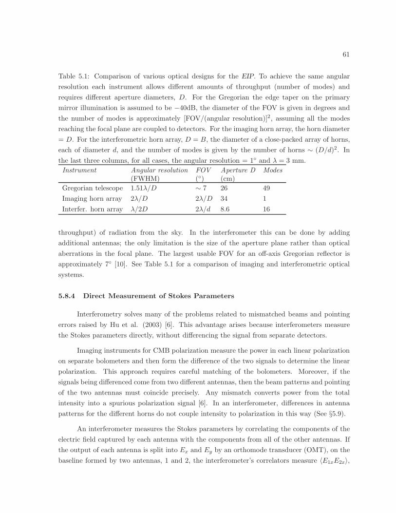
61
Table 5.1: Comparison of various optical designs for the EIP. To achieve the same angular
resolution each instrument allows different amounts of throughput (number of modes) and
requires different aperture diameters, D. For the Gregorian the edge taper on the primary
mirror illumination is assumed to be −40dB, the diameter of the FOV is given in degrees and
the number of modes is approximately [FOV/(angular resolution)]2, assuming all the modes
reaching the focal plane are coupled to detectors. For the imaging horn array, the horn diameter
= D. For the interferometric horn array, D = B, the diameter of a close-packed array of horns,
each of diameter d, and the number of modes is given by the number of horns ∼ (D/d)2. In
the last three columns, for all cases, the angular resolution = 1 and λ = 3 mm.
Instrument Angular resolution FOV Aperture D Modes(FWHM) () (cm)
Gregorian telescope 1.51λ/D ∼ 7 26 49
Imaging horn array 2λ/D 2λ/D 34 1
Interfer. horn array λ/2D 2λ/d 8.6 16
throughput) of radiation from the sky. In the interferometer this can be done by adding
additional antennas; the only limitation is the size of the aperture plane rather than optical
aberrations in the focal plane. The largest usable FOV for an off-axis Gregorian reflector is
approximately 7 [10]. See Table 5.1 for a comparison of imaging and interferometric optical
systems.
5.8.4 Direct Measurement of Stokes Parameters
Interferometry solves many of the problems related to mismatched beams and pointing
errors raised by Hu et al. (2003) [6]. This advantage arises because interferometers measure
the Stokes parameters directly, without differencing the signal from separate detectors.
Imaging instruments for CMB polarization measure the power in each linear polarization
on separate bolometers and then form the difference of the two signals to determine the linear
polarization. This approach requires careful matching of the bolometers. Moreover, if the
signals being differenced come from two different antennas, then the beam patterns and pointing
of the two antennas must coincide precisely. Any mismatch converts power from the total
intensity into a spurious polarization signal [6]. In an interferometer, differences in antenna
patterns for the different horns do not couple intensity to polarization in this way (See §5.9).
An interferometer measures the Stokes parameters by correlating the components of the
electric field captured by each antenna with the components from all of the other antennas. If
the output of each antenna is split into Ex and Ey by an orthomode transducer (OMT), on the
baseline formed by two antennas, 1 and 2, the interferometer’s correlators measure 〈E1xE2x〉,
62
〈E1yE2y〉, 〈E1xE2y〉, and 〈E1yE2x〉. The first two are used to determine I and the latter two
measure U . Rotating the instrument allows a measurement of Q. Stokes V can be recovered in
a similar manner but is expected to be zero for the CMB. Alternatively, the antenna outputs can
be separated into left- and right-circular polarization components by a combination of an OMT
and a polarizer. Correlating these signals also allows recovery of all four Stokes parameters.
DASI uses a switchable polarizer to accomplish this [11].
Separation of E and B Modes. A significant challenge in CMB polarization measurements
is separation of the very weak B modes from the much stronger E modes. Unless a full-sky
map (an impossibility because of Galactic cuts) is made with infinite angular resolution the
two modes “leak” into each other [12, 13]. It has been shown [14, 15], however, that an
interferometer can separate the E and B modes more cleanly than can an imaging experiment,
although detailed calculations of this advantage in realistic simulations remain to be done.
5.9 Systematic Effects
Hu et al. (2003) [6] have reviewed systematic effects relevant to CMB polarization mea-
surements, mainly in the context of imaging instruments. Bunn (2006) [16] performs similar
calculations for interferometers. Table 5.2 outlines a variety of systematic errors and how they
can be managed in imaging and infererometric instruments. The relative importance of these
effects is quite different in interferometric systems: some sources of systematic error in imaging
systems are dramatically reduced in interferometers. As an example we consider the effects of
pointing errors and mismatched antenna patterns.
In a traditional imaging system, the Stokes parameters Q and U are determined by
subtracting the intensities of two different polarizations. For example, Q might be measured by
splitting the incoming radiation into x and y polarizations, determining the intensities Ix and
Iy of the two polarizations, and subtracting. In such an experiment, any mismatch in the beam
patterns used to determine Ix and Iy (including differential pointing errors as well as different
beam shapes) will cause leakage from total power (T ) into polarization (Q,U).
In an interferometer, the signals are combined before squaring to get intensities. In such a
system, mismatched beams do not lead to leakage from temperature into polarization. Suppose
that the signal entering each horn of an interferometer is split into horizontal and vertical
polarizations. Working in the flat-sky approximation, let Eix(r ) and Eiy(r) stand for the x and
y components of the electric field of the radiation entering the ith horn from position r on the
sky. The signals coming out of each horn are averages of the incoming electric fields weighted
by some antenna patterns Gi(x,y)(r).
In an interferometer, these signals are multiplied together to obtain a visibility. To
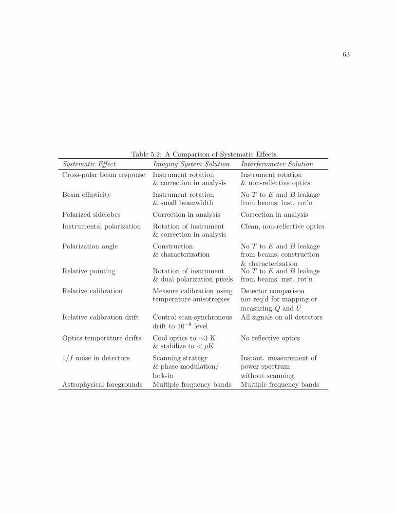
63
Table 5.2: A Comparison of Systematic Effects
Systematic Effect Imaging System Solution Interferometer Solution
Cross-polar beam response Instrument rotation Instrument rotation& correction in analysis & non-reflective optics
Beam ellipticity Instrument rotation No T to E and B leakage& small beamwidth from beams; inst. rot’n
Polarized sidelobes Correction in analysis Correction in analysis
Instrumental polarization Rotation of instrument Clean, non-reflective optics& correction in analysis
Polarization angle Construction No T to E and B leakage& characterization from beams; construction
& characterizationRelative pointing Rotation of instrument No T to E and B leakage
& dual polarization pixels from beams; inst. rot’n
Relative calibration Measure calibration using Detector comparisontemperature anisotropies not req’d for mapping or
measuring Q and URelative calibration drift Control scan-synchronous All signals on all detectors
drift to 10−9 level
Optics temperature drifts Cool optics to ∼3 K No reflective optics& stabilize to < µK
1/f noise in detectors Scanning strategy Instant. measurement of& phase modulation/ power spectrum
lock-in without scanningAstrophysical foregrounds Multiple frequency bands Multiple frequency bands
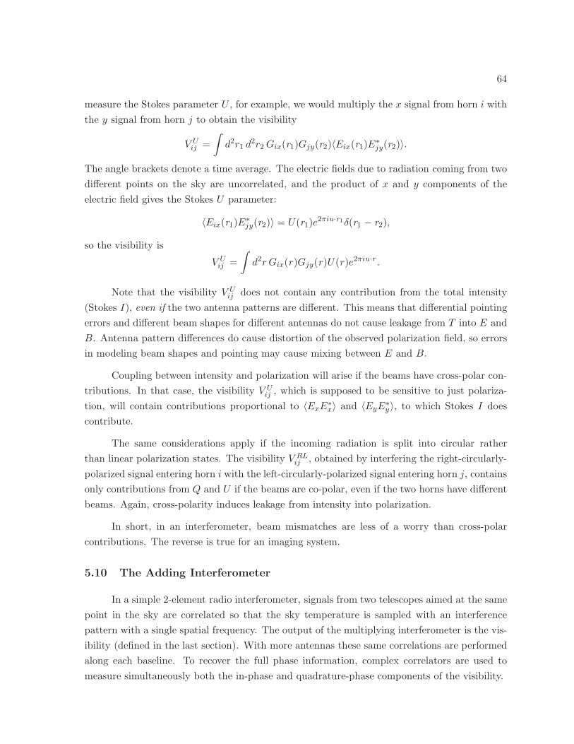
64
measure the Stokes parameter U , for example, we would multiply the x signal from horn i with
the y signal from horn j to obtain the visibility
V Uij =
∫
d2r1 d2r2Gix(r1)Gjy(r2)〈Eix(r1)E
∗jy(r2)〉.
The angle brackets denote a time average. The electric fields due to radiation coming from two
different points on the sky are uncorrelated, and the product of x and y components of the
electric field gives the Stokes U parameter:
〈Eix(r1)E∗jy(r2)〉 = U(r1)e
2πiu·r1δ(r1 − r2),
so the visibility is
V Uij =
∫
d2r Gix(r)Gjy(r)U(r)e2πiu·r .
Note that the visibility V Uij does not contain any contribution from the total intensity
(Stokes I), even if the two antenna patterns are different. This means that differential pointing
errors and different beam shapes for different antennas do not cause leakage from T into E and
B. Antenna pattern differences do cause distortion of the observed polarization field, so errors
in modeling beam shapes and pointing may cause mixing between E and B.
Coupling between intensity and polarization will arise if the beams have cross-polar con-
tributions. In that case, the visibility V Uij , which is supposed to be sensitive to just polariza-
tion, will contain contributions proportional to 〈ExE∗x〉 and 〈EyE∗
y〉, to which Stokes I does
contribute.
The same considerations apply if the incoming radiation is split into circular rather
than linear polarization states. The visibility V RLij , obtained by interfering the right-circularly-
polarized signal entering horn i with the left-circularly-polarized signal entering horn j, contains
only contributions from Q and U if the beams are co-polar, even if the two horns have different
beams. Again, cross-polarity induces leakage from intensity into polarization.
In short, in an interferometer, beam mismatches are less of a worry than cross-polar
contributions. The reverse is true for an imaging system.
5.10 The Adding Interferometer
In a simple 2-element radio interferometer, signals from two telescopes aimed at the same
point in the sky are correlated so that the sky temperature is sampled with an interference
pattern with a single spatial frequency. The output of the multiplying interferometer is the vis-
ibility (defined in the last section). With more antennas these same correlations are performed
along each baseline. To recover the full phase information, complex correlators are used to
measure simultaneously both the in-phase and quadrature-phase components of the visibility.
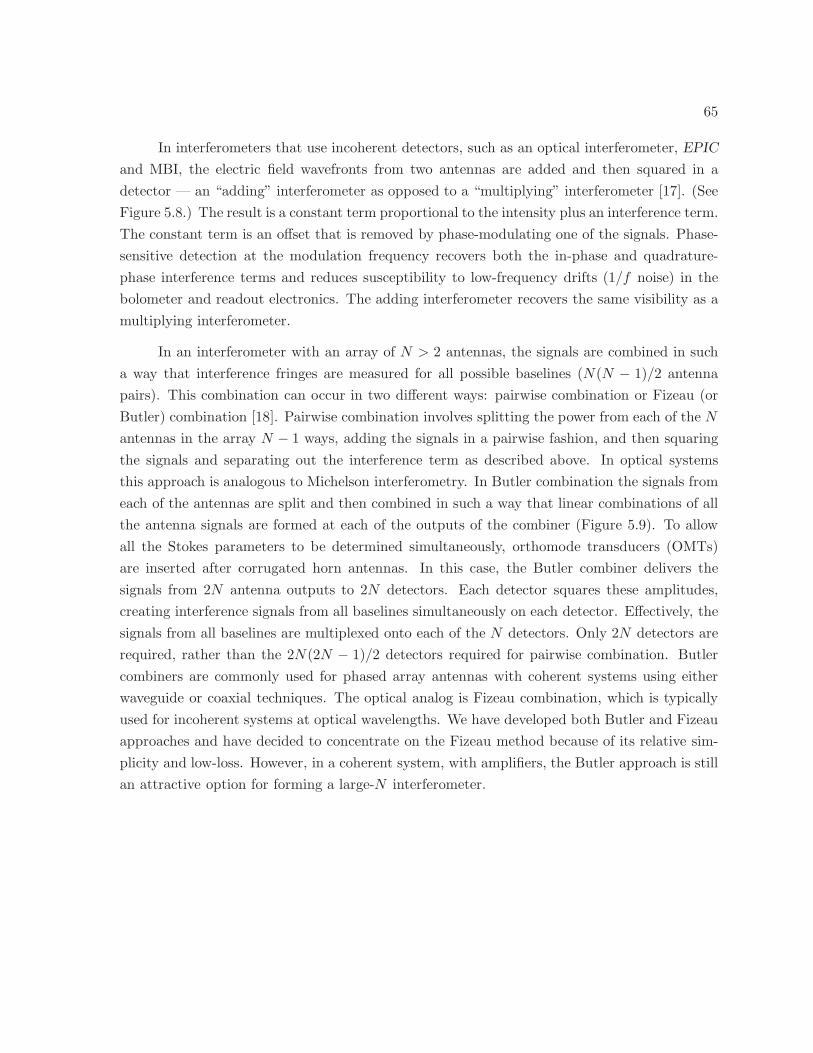
65
In interferometers that use incoherent detectors, such as an optical interferometer, EPIC
and MBI, the electric field wavefronts from two antennas are added and then squared in a
detector — an “adding” interferometer as opposed to a “multiplying” interferometer [17]. (See
Figure 5.8.) The result is a constant term proportional to the intensity plus an interference term.
The constant term is an offset that is removed by phase-modulating one of the signals. Phase-
sensitive detection at the modulation frequency recovers both the in-phase and quadrature-
phase interference terms and reduces susceptibility to low-frequency drifts (1/f noise) in the
bolometer and readout electronics. The adding interferometer recovers the same visibility as a
multiplying interferometer.
In an interferometer with an array of N > 2 antennas, the signals are combined in such
a way that interference fringes are measured for all possible baselines (N(N − 1)/2 antenna
pairs). This combination can occur in two different ways: pairwise combination or Fizeau (or
Butler) combination [18]. Pairwise combination involves splitting the power from each of the N
antennas in the array N − 1 ways, adding the signals in a pairwise fashion, and then squaring
the signals and separating out the interference term as described above. In optical systems
this approach is analogous to Michelson interferometry. In Butler combination the signals from
each of the antennas are split and then combined in such a way that linear combinations of all
the antenna signals are formed at each of the outputs of the combiner (Figure 5.9). To allow
all the Stokes parameters to be determined simultaneously, orthomode transducers (OMTs)
are inserted after corrugated horn antennas. In this case, the Butler combiner delivers the
signals from 2N antenna outputs to 2N detectors. Each detector squares these amplitudes,
creating interference signals from all baselines simultaneously on each detector. Effectively, the
signals from all baselines are multiplexed onto each of the N detectors. Only 2N detectors are
required, rather than the 2N(2N − 1)/2 detectors required for pairwise combination. Butler
combiners are commonly used for phased array antennas with coherent systems using either
waveguide or coaxial techniques. The optical analog is Fizeau combination, which is typically
used for incoherent systems at optical wavelengths. We have developed both Butler and Fizeau
approaches and have decided to concentrate on the Fizeau method because of its relative sim-
plicity and low-loss. However, in a coherent system, with amplifiers, the Butler approach is still
an attractive option for forming a large-N interferometer.
66
Figure 5.8: Adding interferometer. At antenna A2 the electric field is E0, and at A1 it is E0eiφ,
where φ = kB sinα and k = 2π/λ. B is the length of the baseline, and α is the angle of the
source with respect to the symmetry axis of the baseline, as shown. (For simplicity consider
only one wavelength, λ, and ignore time dependent factors.) In a multiplying interferometer
the in-phase output of the correlator is proportional to E20 cosφ. For the adding interferometer,
the output is proportional to E20 +E2
0 cos(φ+ ∆φ(t)). Modulation of ∆φ(t) allows the recovery
of the interference term, E20 cosφ, which is proportional to the visibility of the baseline.
Figure 5.9: Block diagram of a planned CMB polarization experiment. Light enters the instru-
ment from the left. Each phase switch is modulated in a sequence that allows recovery of the
interference terms (visibilities) by phase-sensitive detection at the detectors. The signals are
mixed in the beam combiner and detected on cold bolometers at the right. The beam combiner
can be implemented either using guided waves (Butler combiner, as shown here) or quasiopti-
cally (Fizeau combiner, see below). The triangles represent corrugated conical horn antennas,
which connect through transitions to rectangular waveguide. Orthomode transducers (OMTs)
allow all the Stokes parameters to be determined simultaneously.
67
Bibliography
[1] K. Rohlfs and T. L. Wilson, Tools of Radio Astronomy, Tools of Radio Astronomy, XVI,
423 pp. 127 figs., 20 tabs.. Springer-Verlag Berlin Heidelberg New York. Also Astronomy
and Astrophysics Library, 1996.
[2] C. Calderon, “SIMULATION OF THE PERFORMANCE OF THE MILLIMETRE-
WAVE BOLOMETRIC INTERFEROMETER (MBI) FOR COSMIC MICROWAVE
BACKGROUND OBSERVATIONS. Ph.D. Thesis, Cardiff.,” Ph.D. Thesis, 2006.
[3] Jaiseung Kim, “The Millimeter-wave Bolometric Interferometer (MBI) for Observing the
Cosmic Microwave Background Polarization,” Ph.D. Thesis, 2006.
[4] M. White, J. E. Carlstrom, M. Dragovan, and W. L. Holzapfel, “Interferometric Obser-
vation of Cosmic Microwave Background Anisotropies,” ApJ, vol. 514, pp. 12–24, Mar.
1999.
[5] Paul F. Goldsmith, Quasioptical Systems, IEEE Press, 1998.
[6] W. Hu, M. M. Hedman, and M. Zaldarriaga, “Benchmark parameters for CMB polarization
experiments,” Phys. Rev. D, vol. 67, no. 4, pp. 043004–+, Feb. 2003.
[7] L. Knox and Y.-S. Song, “Limit on the Detectability of the Energy Scale of Inflation,”
Physical Review Letters, vol. 89, no. 1, pp. 011303–+, July 2002.
[8] E. Carretti, R. Tascone, S. Cortiglioni, J. Monari, and M. Orsini, “Limits due to instru-
mental polarisation in CMB experiments at microwave wavelengths,” New Astronomy, vol.
6, pp. 173–187, May 2001.
[9] E. Carretti, S. Cortiglioni, C. Sbarra, and R. Tascone, “Antenna instrumental polarization
and its effects on E- and B-modes for CMBP observations,” Astronomy & Astrophysics,
vol. 420, pp. 437–445, June 2004.
[10] S. Hanany and D. P. Marrone, “Comparison of designs of off-axis Gregorian telescopes for
millimeter-wave large focal-plane arrays,” Appl. Opt., vol. 41, pp. 4666–4670, Aug. 2002.
68
[11] E. M. Leitch, J. M. Kovac, C. Pryke, J. E. Carlstrom, N. W. Halverson, W. L. Holzapfel,
M. Dragovan, B. Reddall, and E. S. Sandberg, “Measurement of polarization with the
Degree Angular Scale Interferometer,” Nature, vol. 420, pp. 763–771, Dec. 2002.
[12] A. Lewis, A. Challinor, and N. Turok, “Analysis of CMB polarization on an incomplete
sky,” Phys. Rev. D, vol. 65, no. 2, pp. 023505–+, Jan. 2002.
[13] E. F. Bunn, “Separating E from B,” New Astronomy Review, vol. 47, pp. 987–994, Dec.
2003.
[14] C.-G. Park, K.-W. Ng, C. Park, G.-C. Liu, and K. Umetsu, “Observational Strategies
of Cosmic Microwave Background Temperature and Polarization Interferometry Experi-
ments,” ApJ, vol. 589, pp. 67–81, May 2003.
[15] C.-G. Park and K.-W. Ng, “E/B Separation in Cosmic Microwave Background Interfer-
ometry,” ApJ, vol. 609, pp. 15–21, July 2004.
[16] E. F. Bunn, “Systematic Errors in Microwave Background Interferometry,” to be submitted
to Phys. Rev. D., 2006.
[17] K. Rohlfs and T. L. Wilson, Tools of Radio Astronomy, Springer, 2004.
[18] J. Zmuidzinas, “Cramer-Rao sensitivity limits for astronomical instruments: implications
for interferometer design,” Optical Society of America Journal A, vol. 20, pp. 218–233,
Feb. 2003.
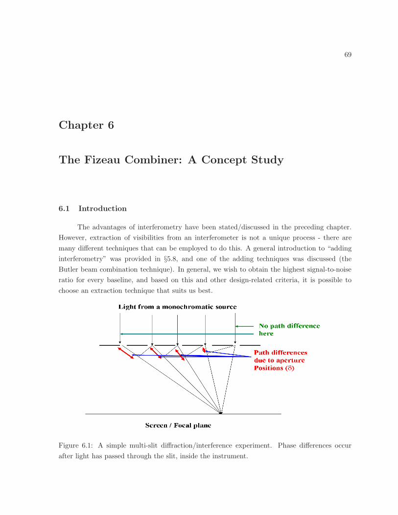
69
Chapter 6
The Fizeau Combiner: A Concept Study
6.1 Introduction
The advantages of interferometry have been stated/discussed in the preceding chapter.
However, extraction of visibilities from an interferometer is not a unique process - there are
many different techniques that can be employed to do this. A general introduction to “adding
interferometry” was provided in §5.8, and one of the adding techniques was discussed (the
Butler beam combination technique). In general, we wish to obtain the highest signal-to-noise
ratio for every baseline, and based on this and other design-related criteria, it is possible to
choose an extraction technique that suits us best.
Figure 6.1: A simple multi-slit diffraction/interference experiment. Phase differences occur
after light has passed through the slit, inside the instrument.
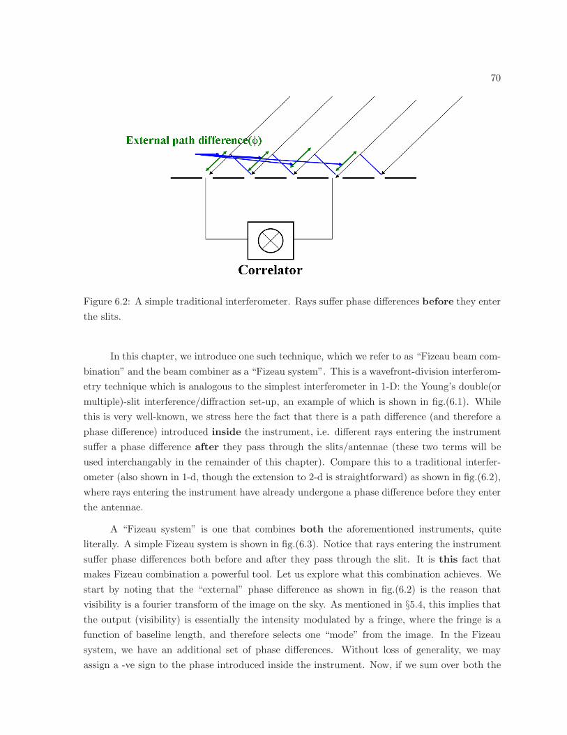
70
Figure 6.2: A simple traditional interferometer. Rays suffer phase differences before they enter
the slits.
In this chapter, we introduce one such technique, which we refer to as “Fizeau beam com-
bination” and the beam combiner as a “Fizeau system”. This is a wavefront-division interferom-
etry technique which is analogous to the simplest interferometer in 1-D: the Young’s double(or
multiple)-slit interference/diffraction set-up, an example of which is shown in fig.(6.1). While
this is very well-known, we stress here the fact that there is a path difference (and therefore a
phase difference) introduced inside the instrument, i.e. different rays entering the instrument
suffer a phase difference after they pass through the slits/antennae (these two terms will be
used interchangably in the remainder of this chapter). Compare this to a traditional interfer-
ometer (also shown in 1-d, though the extension to 2-d is straightforward) as shown in fig.(6.2),
where rays entering the instrument have already undergone a phase difference before they enter
the antennae.
A “Fizeau system” is one that combines both the aforementioned instruments, quite
literally. A simple Fizeau system is shown in fig.(6.3). Notice that rays entering the instrument
suffer phase differences both before and after they pass through the slit. It is this fact that
makes Fizeau combination a powerful tool. Let us explore what this combination achieves. We
start by noting that the “external” phase difference as shown in fig.(6.2) is the reason that
visibility is a fourier transform of the image on the sky. As mentioned in §5.4, this implies that
the output (visibility) is essentially the intensity modulated by a fringe, where the fringe is a
function of baseline length, and therefore selects one “mode” from the image. In the Fizeau
system, we have an additional set of phase differences. Without loss of generality, we may
assign a -ve sign to the phase introduced inside the instrument. Now, if we sum over both the
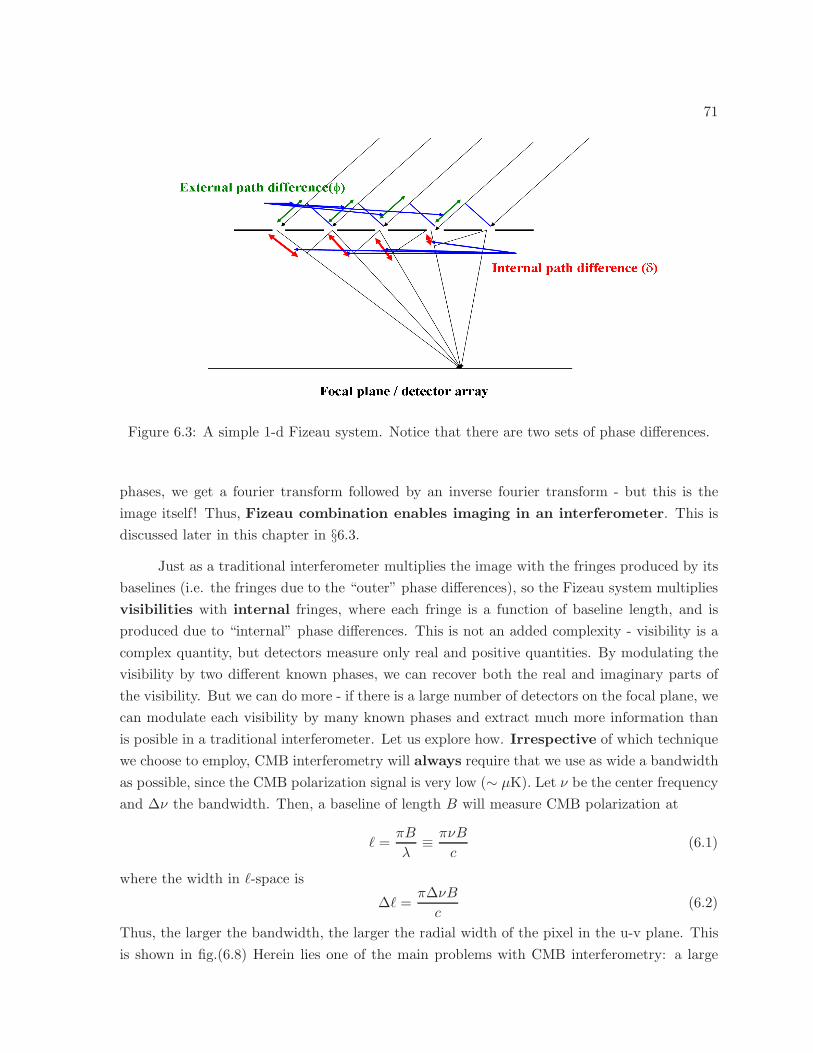
71
Figure 6.3: A simple 1-d Fizeau system. Notice that there are two sets of phase differences.
phases, we get a fourier transform followed by an inverse fourier transform - but this is the
image itself! Thus, Fizeau combination enables imaging in an interferometer. This is
discussed later in this chapter in §6.3.
Just as a traditional interferometer multiplies the image with the fringes produced by its
baselines (i.e. the fringes due to the “outer” phase differences), so the Fizeau system multiplies
visibilities with internal fringes, where each fringe is a function of baseline length, and is
produced due to “internal” phase differences. This is not an added complexity - visibility is a
complex quantity, but detectors measure only real and positive quantities. By modulating the
visibility by two different known phases, we can recover both the real and imaginary parts of
the visibility. But we can do more - if there is a large number of detectors on the focal plane, we
can modulate each visibility by many known phases and extract much more information than
is posible in a traditional interferometer. Let us explore how. Irrespective of which technique
we choose to employ, CMB interferometry will always require that we use as wide a bandwidth
as possible, since the CMB polarization signal is very low (∼ µK). Let ν be the center frequency
and ∆ν the bandwidth. Then, a baseline of length B will measure CMB polarization at
ℓ =πB
λ≡ πνB
c(6.1)
where the width in ℓ-space is
∆ℓ =π∆νB
c(6.2)
Thus, the larger the bandwidth, the larger the radial width of the pixel in the u-v plane. This
is shown in fig.(6.8) Herein lies one of the main problems with CMB interferometry: a large
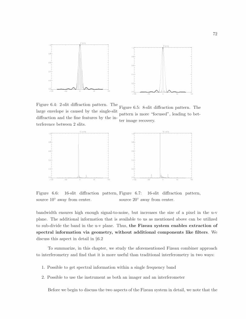
72
Figure 6.4: 2-slit diffraction pattern. The
large envelope is caused by the single-slit
diffraction and the fine features by the in-
terference between 2 slits.
Figure 6.5: 8-slit diffraction pattern. The
pattern is more “focused”, leading to bet-
ter image recovery.
Figure 6.6: 16-slit diffraction pattern,
source 10 away from center.
Figure 6.7: 16-slit diffraction pattern,
source 20 away from center.
bandwidth ensures high enough signal-to-noise, but increases the size of a pixel in the u-v
plane. The additional information that is available to us as mentioned above can be utilized
to sub-divide the band in the u-v plane. Thus, the Fizeau system enables extraction of
spectral information via geometry, without additional components like filters. We
discuss this aspect in detail in §6.2
To summarize, in this chapter, we study the aforementioned Fizeau combiner approach
to interferometry and find that it is more useful than traditional interferometry in two ways:
1. Possible to get spectral information within a single frequency band
2. Possible to use the instrument as both an imager and an interferometer
Before we begin to discuss the two aspects of the Fizeau system in detail, we note that the
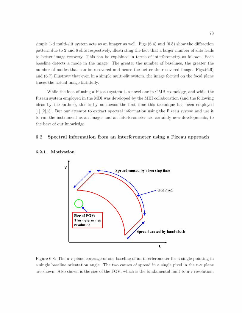
73
simple 1-d multi-slit system acts as an imager as well. Figs.(6.4) and (6.5) show the diffraction
pattern due to 2 and 8 slits respectively, illustrating the fact that a larger number of slits leads
to better image recovery. This can be explained in terms of interferometry as follows. Each
baseline detects a mode in the image. The greater the number of baselines, the greater the
number of modes that can be recovered and hence the better the recovered image. Figs.(6.6)
and (6.7) illustrate that even in a simple multi-slit system, the image formed on the focal plane
traces the actual image faithfully.
While the idea of using a Fizeau system is a novel one in CMB cosmology, and while the
Fizeau system employed in the MBI was developed by the MBI collaboration (and the following
ideas by the author), this is by no means the first time this technique has been employed
[1],[2],[3]. But our attempt to extract spectral information using the Fizeau system and use it
to run the instrument as an imager and an interferometer are certainly new developments, to
the best of our knowledge.
6.2 Spectral information from an interferometer using a Fizeau approach
6.2.1 Motivation
Figure 6.8: The u-v plane coverage of one baseline of an interferometer for a single pointing in
a single baseline orientation angle. The two causes of spread in a single pixel in the u-v plane
are shown. Also shown is the size of the FOV, which is the fundamental limit to u-v resolution.
74
As mentioned earlier in the chapter, cosmological signals are very weak; therefore, a
wide bandwidth helps increase the power input from the cosmological source. However, a
wide bandwidth also means poor u-v coverage as shown in fig.(5.4) and fig.(6.8). This can be
explained as follows. Consider a two-slit experiment with a monochromatic point source. This
experiment yields fringes that can be computed given the exact parameters of the experiment.
Now, if the same point source emits two different wavelengths that differ by a small percentage,
the fringes are slightly shifted. If a lot of such wavelengths are used, each only slightly different
than the one preceding it, then a “fringe-band” is produced instead of clear, sharp fringes. We
call this effect a “fringe wash-out”. The wider the bandwidth, the greater the wash-out.
Now, a single sharp (i.e. monochromatic) fringe corresponds to a single point on the u-v
plane. If the effect of the bandwidth is to add many such fringes, what it means is that we are
measuring the average visibility over a certain finite area on the u-v plane, where the radial
stretch is due to a finite bandwidth and the angular stretch represents the integration time for
the interferometer.
6.2.2 Preliminaries
The output measured at the bolometers in MBI contains the following phase information
integrated over the entire bandwidth (75− 110GHz)
1. Phase introduced because of the path difference between any two rays that arrive from
the same part of the sky on the the two outward-facing antennae that make up a baseline
2. Phase introduced because of the path difference between any two rays that arrive from
two different antennae on to the same point in the focal plane
The phase in point 1 is due to the fact that MBI is an interferometer, and so the visibility that
we measure must, by definition, include this phase. However, the phase in 2 above introduced
by the beam combiner needs to be eliminated to recover visibility from each bolometer. If
there were a way to calculate the net phase introduced by the beam combiner over the whole
bandwidth, then all we would need to do is to divide the output at each point in the focal plane
by this net phase, and we would get visibility directly.
However, calculating this net phase is not easy, since integration over the bandwidth
turns our calculation into an unrecognizable beast. So we choose instead to work with fringe
patterns1. In order to do so, we need to realize that what we observe at every detector is the
visibility on the sky times the phase factor, summed over a part of the fringe pattern.
1This is exactly the same as saying that the visibilities in each sub-band are modulated by a fringe which
depends on baseline length. To extract these visibilities, we need to separate out the fringes.
75
But the fringe pattern is different for every single frequency in the bandwidth. Visibility
is also different for every different frequency. This can be reasoned as follows. Every single
frequency defines a single value of ℓ for a single baseline as follows. The angular resolution of
a single baseline of length D is
∆θ =λ
D
⇒ ℓ =2π
∆θ
=2πD
λ
⇒ ℓ =2πDν
c(6.3)
Thus, a range of values of ν will produce a range of ℓ’s, or a band in ℓ-space. A finite-bandwidth
interferometer thus measures what is called a “bandpower” instead of a single value of the power
spectrum at one value of ℓ. But the power spectrum is just the variance of the visibilities for
a circle (ring) in the u − v plane, as proved in the previous chapter. And so we get different
visibilities for the same baseline and orientation but for different frequencies [fig. 4.8?].
We can therefore think of the effect of the instrument on the visibilities in the following
way. Let us divide the entire bandwidth of the instrument into N sub-bands and let ν1, ν2...νN
be the centre-frequencies of these N sub-bands. Then for one baseline, one orientation, and
one detector position, these will correspond to visibilities V1, V2...VN and to phase differences
φj1, φj2...φjN (where j represents the detector). If we represent the output at the jth detector
as O then we get
Oj =
N∑
α=0
Vαeiφjα (6.4)
Given just one detector, it is impossible to extract every Vα for every sub-band, even though we
know precisely what the φjα’s are. However, if we have N detectors, then we can easily write
the following system of equations
O1 = V1eiφ11 + V2e
iφ12 + · · ·+ VNeiφ1N
O2 = V1eiφ21 + V2e
iφ22 + · · ·+ VNeiφ2N
. . .
ON = V1eiφN1 + V2e
iφN2 + · · ·+ VNeiφNN (6.5)
This is a system of N equations with N unknowns - V1, V2 · · · VN , and so we can get the values
for each one of these “sub-band visibilities”. The beam combiner thus achieves far more than
just separating the real and imaginary parts of visibilities. (In fact, there are 2N equations,
since visibilities are complex quantities, but this has been overlooked to simplify the equations
for the discussion).
76
6.2.3 Effect of non-zero detector size
In the discussion above, we assumed that the collection area of the detectors is negligible,
and we completely ignored the effect of the fringe pattern. Let us account for these effects
in the following way. Let A be the effective collecting area of each detector. Let f (x, να) be
the value of the fringe pattern (i.e. just a fraction) at a point on the focal plane x and in a
frequency sub-band marked by α. Then, equations (6.5) become
O1 =
∫
V1eiφ11(x)f (x, ν1) d
2x + · · ·+∫
VNeiφ1N (x)f (x, νN ) d2x
O2 =
∫
V1eiφ21(x)f (x, ν1) d
2x + · · ·+∫
VNeiφ2N (x)f (x, νN ) d2x
. . .
ON =
∫
V1eiφN1(x)f (x, ν1) d
2x + · · ·+∫
VNeiφNN (x)f (x, νN ) d2x (6.6)
where it is understood that integration is done over the area of the detector.
This still leaves us with a problem - that of deconvolving the V ’s from the integrals.
However, if the area of the detector is small compared to the width of fringes, then we can
assume that the phase differences remain roughly constant over the collecting area of one
detector, so that we may write
O1 = A[
V1eiφ11(x)F (x, ν1) + · · · + VNe
iφ1N (x)F (x, νN )]
O2 = A[
V1eiφ21(x)F (x, ν1) + · · · + VNe
iφ2N (x)F (x, νN )]
. . .
ON = A[
V1eiφN1(x)F (x, ν1) + · · · + VNe
iφNN (x)F (x, νN )]
(6.7)
where F (x, να) represents an “average” value of the fringe pattern, perhaps the value at the
centre of the detector.
Equations (6.7) again have N variables and can be solved to get N visibilities over the
bandwidth.
6.2.4 Feasibility of using techniques in §6.2 for MBI
1. Bandwidth Issues
For MBI, we are using ∼ 20 detectors, meaning that we can extract visibilities for 20
“sub-bands”. Bandwidth for MBI is 35 GHz, so that the width of every sub-band is 1.75
GHz, such that we get, for every sub-band
∆ν
ν=
1.75
90∼ 0.002 (6.8)
which is really small. Thus, the small-bandwidth approximation holds for equations (6.7).
77
2. Detector Area Issues
We need to compare the area of every detector to the width of the fringes, in order to
estimate whether the area approximation holds in equations (6.7). We first estimate the
width of fringes on the focal plane thus (distance to focal plane = L ∼ 1m):
∆w =λ
DL ∼ 0.3
10× 1m ∼ 3cm (6.9)
The diameter of a detector area is ∼ 1” ≡ 2.54 cm, so that one detector covers about
one entire fringe. This reduces the spectral resolution that can be obtained using this
technique with MBI-4. Future versions of MBI will have much smaller collecting areas,
and will thus provide better resolution.
6.3 The Fizeau combiner as an imager
In addition to acting as an interferometer, the Fizeau system can also be used directly
as an imager and additionally be used to extract spectral information in the u-v plane not
normally possible with conventional interferometer systems. But how is this possible? After
all, an interferometer chooses certain fourier modes specified by the lengths of its baselines.
However, in the Fizeau system, every fourier mode from every baseline falls on every detector
in the focal plane. In addition, the phase differences introduced within the instrument correct
for the phase differences introduced outside the system. This way, every detector detects ALL
possible modes in the right phase - but this is exactly a part of the image!
Thus, the Fizeau system acts naturally as an imager. As a matter of fact, one has to
make a greater effort to operate it in the interferometer mode, for precisely the reason mentioned
above - that the output from every baseline occurs at every detector. So, in order to be able to
distinguish between visibilities from different baselines at every detector, we need another level
of modulation. We use a phase modulator based on the Faraday Effect, and discuss it in the
following chapter. A more detailed discussion and mathematical description of the operation
of this phase modulator combined with the Fizeau system will be provided in a subsequent
publication.
In what follows, we denote the output at the bolometers as O and a fourier transform as
F.
Let ǫ be the phase difference introduced outside the instrument and δ the phase difference
inside the instrument. If E1 and E2 are the electric fields at the two antennae that make a
baseline, then the output from one baseline at any detector is:
O =
∫ θ2
θ=θ1
∫ φ2
φ=φ1
E∗1E2e
i(δ+ǫ) + E1E∗2e
−i(δ+ǫ) sin θdφdθ (6.10)
78
The units of this “intermediate” visibility are Wm−2Hz−1, since we have integrated over the
solid angle.
Equivalently,
O =
∫ θ2
θ=θ1
∫ φ2
φ=φ1
2ℜ(
E∗1E2e
i(δ+ǫ))
sin θdφdθ (6.11)
O ≈∫ θ2
θ=θ1
∫ φ2
φ=φ1
2ℜ(
E∗1E2e
i(δ+ǫ))
dφdθ (6.12)
in the flat-sky case. We can now integrate over the focal-plane area in the following way: if the
area on the focal plane being integrated over is AF , then
O ≈ 1
AF
∫ ∫ ∫ θ2
θ=θ1
∫ φ2
φ=φ1
2ℜ(
E∗1E2e
i(δ(x,y)+ǫ(θ,φ)))
dφdθdxdy (6.13)
Let us consider just one term in the expression ℜ (...):
O ≈ 1
AF
∫ ∫ ∫ θ2
θ=θ1
∫ φ2
φ=φ1
(
E∗1E2e
iǫ(θ,φ))
dφdθe−iδ(x,y)dxdy (6.14)
where we have changed the sign on δ without loss of generality, since phase differences inside
the cryostat are independent of phases due to the skyward horn antennae.
Now, E1E∗2 ∝ IS where IS is a linear combination of Stokes’ parameters[3]. In addition,
we need to take into account the antenna beam:
E1E∗2 ∝ B (θ, φ) IS (6.15)
We can thus write
O =1
AF
∫ ∫
B (x, y)
∫ ∫
B (θ, φ) ISeiǫ(θ,φ)dθdφe−iδ(x,y)dxdy (6.16)
Now, if ǫ (θ, φ) is linear in θ and φ (this is true in the flat-sky case), then
O =1
AF
∫ ∫
B (x, y)F (BIS) e−iδ(x,y)dxdy (6.17)
Now, if the distance from the inward-facing antennae to the focal plane ≫ the collecting area
for each bolometer, δ (x, y) is linear in (x, y) and
O =1
AFF−1 (BF (BIS)) (6.18)
IF this is correct, the beam needs to be deconvolved from the above expression in order to
obtain the image from MBI.
Now, eq(6.17) can be split up over the focal plane:
O =1
AF
[∫ ∫
1BF (BIS) e−iδ(x,y) + · · ·+
∫ ∫
NBF (BIS) e−iδ(x,y)
]
(6.19)
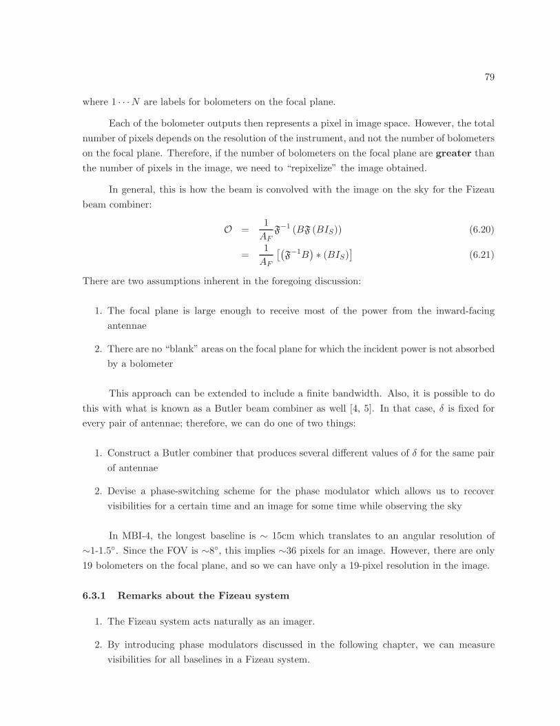
79
where 1 · · ·N are labels for bolometers on the focal plane.
Each of the bolometer outputs then represents a pixel in image space. However, the total
number of pixels depends on the resolution of the instrument, and not the number of bolometers
on the focal plane. Therefore, if the number of bolometers on the focal plane are greater than
the number of pixels in the image, we need to “repixelize” the image obtained.
In general, this is how the beam is convolved with the image on the sky for the Fizeau
beam combiner:
O =1
AFF−1 (BF (BIS)) (6.20)
=1
AF
[(F−1B
)∗ (BIS)
](6.21)
There are two assumptions inherent in the foregoing discussion:
1. The focal plane is large enough to receive most of the power from the inward-facing
antennae
2. There are no “blank” areas on the focal plane for which the incident power is not absorbed
by a bolometer
This approach can be extended to include a finite bandwidth. Also, it is possible to do
this with what is known as a Butler beam combiner as well [4, 5]. In that case, δ is fixed for
every pair of antennae; therefore, we can do one of two things:
1. Construct a Butler combiner that produces several different values of δ for the same pair
of antennae
2. Devise a phase-switching scheme for the phase modulator which allows us to recover
visibilities for a certain time and an image for some time while observing the sky
In MBI-4, the longest baseline is ∼ 15cm which translates to an angular resolution of
∼1-1.5. Since the FOV is ∼8, this implies ∼36 pixels for an image. However, there are only
19 bolometers on the focal plane, and so we can have only a 19-pixel resolution in the image.
6.3.1 Remarks about the Fizeau system
1. The Fizeau system acts naturally as an imager.
2. By introducing phase modulators discussed in the following chapter, we can measure
visibilities for all baselines in a Fizeau system.
80
3. The Fizeau system makes it possible to recover spectral information without the need for
filters.
While it is possible to divide the bandwidth into many different sub-bandwidths, it isn’t
possible to do this indefinitely. The beam for a single antenna determines the FOV of the
instrument and limits the resolution in the u-v plane, as shown in fig.(6.9).
u
v
Fine repixelization due to Fizeau combiner
Beam of single antenna
Figure 6.9: The u-v coverage of a single baseline has been divided into many pixels; however,
the beam of a single antenna is larger than a single pixel, so that this division is not physical.
There exists a way to reduce the effective u-v beamsize below that determined by the
FOV: “super-resolution coverage”. Further discussion on this is left to a future publication.
It is also possible to operate the interferometer simultaneously as an imager. The
additional modulation mentioned above opens up a range of possibilities, including the simul-
taneous measurement of visibilities and images. This shall also be explored further in a future
publication.
In conclusion, the Fizeau system introduced here is a powerful tool for CMB cosmology:
it allows the recovery of more information than is possible with traditional interferometers or

81
imagers and does not need significantly more resources to build. A discussion of the simulation
of a simple Fizeau system is given in §8.2.
82
Bibliography
[1] D. Loreggia, D. Gardiol, M. Gai, M. G. Lattanzi, and D. Busonero, “Fizeau interferom-
etry from space: a challenging frontier in global astrometry,” in New Frontiers in Stellar
Interferometry, Proceedings of SPIE Volume 5491. Edited by Wesley A. Traub. Bellingham,
WA: The International Society for Optical Engineering, 2004., p.255, W. A. Traub, Ed.,
Oct. 2004, vol. 5491 of Presented at the Society of Photo-Optical Instrumentation Engineers
(SPIE) Conference, pp. 255–+.
[2] M. R. Swain, C. K. Walker, M. Dragovan, P. J. Dumont, P. R. Lawson, E. Serabyn, and
H. W. Yorke, “A Fizeau Spatial-Spectral Imaging Submillimeter Interferometer for the
Large Binocular Telescope,” in Bulletin of the American Astronomical Society, Dec. 2002,
vol. 34 of Bulletin of the American Astronomical Society, pp. 1302–+.
[3] M. L. Cobb, “A Comparison of Michelson and Fizeau Beam Combiners for Optical Inter-
ferometry,” in Bulletin of the American Astronomical Society, Dec. 2000, vol. 32 of Bulletin
of the American Astronomical Society, pp. 1429–+.
[4] J. Zmuidzinas, “Cramer-rao sensitivity limits for astronomical instruments:implications for
interferometer design,” J. Opt. Soc. Am. A, vol. 20, no. 2, pp. 218, 2003.
[5] C. Calderon, “SIMULATION OF THE PERFORMANCE OF THE MILLIMETRE-WAVE
BOLOMETRIC INTERFEROMETER (MBI) FOR COSMIC MICROWAVE BACK-
GROUND OBSERVATIONS. Ph.D. Thesis, Cardiff.,” Ph.D. Thesis, 2006.
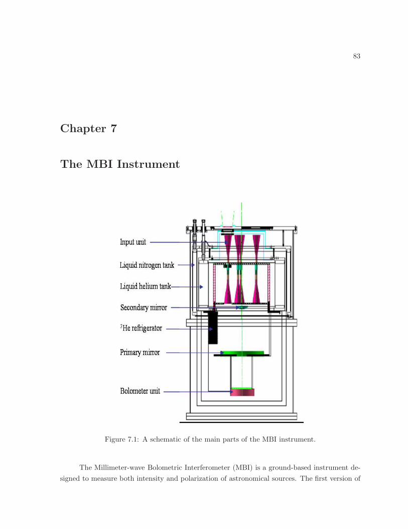
83
Chapter 7
The MBI Instrument
Figure 7.1: A schematic of the main parts of the MBI instrument.
The Millimeter-wave Bolometric Interferometer (MBI) is a ground-based instrument de-
signed to measure both intensity and polarization of astronomical sources. The first version of
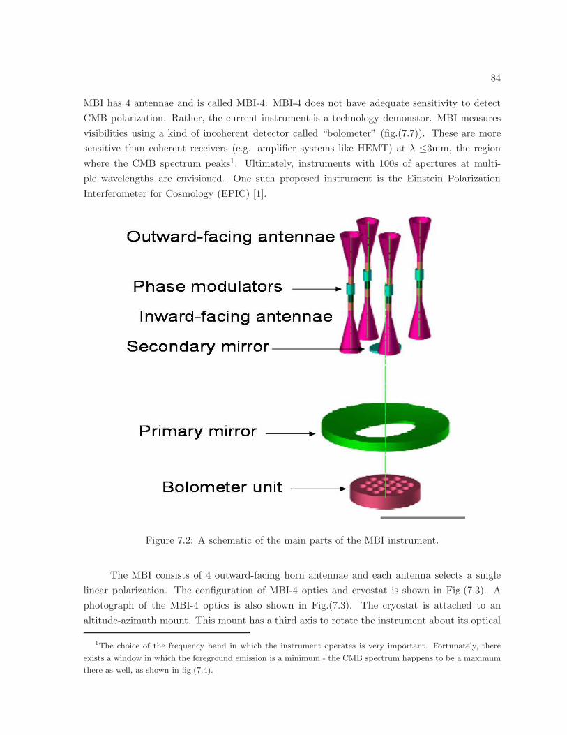
84
MBI has 4 antennae and is called MBI-4. MBI-4 does not have adequate sensitivity to detect
CMB polarization. Rather, the current instrument is a technology demonstor. MBI measures
visibilities using a kind of incoherent detector called “bolometer” (fig.(7.7)). These are more
sensitive than coherent receivers (e.g. amplifier systems like HEMT) at λ ≤3mm, the region
where the CMB spectrum peaks1. Ultimately, instruments with 100s of apertures at multi-
ple wavelengths are envisioned. One such proposed instrument is the Einstein Polarization
Interferometer for Cosmology (EPIC) [1].
Figure 7.2: A schematic of the main parts of the MBI instrument.
The MBI consists of 4 outward-facing horn antennae and each antenna selects a single
linear polarization. The configuration of MBI-4 optics and cryostat is shown in Fig.(7.3). A
photograph of the MBI-4 optics is also shown in Fig.(7.3). The cryostat is attached to an
altitude-azimuth mount. This mount has a third axis to rotate the instrument about its optical
1The choice of the frequency band in which the instrument operates is very important. Fortunately, there
exists a window in which the foreground emission is a minimum - the CMB spectrum happens to be a maximum
there as well, as shown in fig.(7.4).
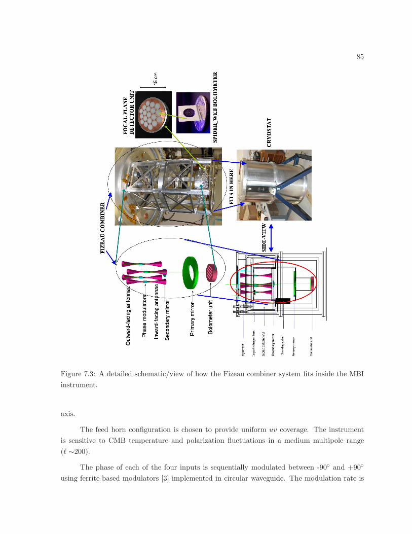
85
Figure 7.3: A detailed schematic/view of how the Fizeau combiner system fits inside the MBI
instrument.
axis.
The feed horn configuration is chosen to provide uniform uv coverage. The instrument
is sensitive to CMB temperature and polarization fluctuations in a medium multipole range
(ℓ ∼200).
The phase of each of the four inputs is sequentially modulated between -90 and +90
using ferrite-based modulators [3] implemented in circular waveguide. The modulation rate is
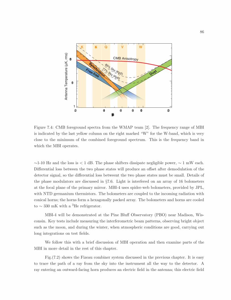
86
Figure 7.4: CMB foreground spectra from the WMAP team [2]. The frequency range of MBI
is indicated by the last yellow column on the right marked “W” for the W-band, which is very
close to the minimum of the combined foreground spectrum. This is the frequency band in
which the MBI operates.
∼1-10 Hz and the loss is < 1 dB. The phase shifters dissipate negligible power, ∼ 1 mW each.
Differential loss between the two phase states will produce an offset after demodulation of the
detector signal, so the differential loss betweent the two phase states must be small. Details of
the phase modulators are discussed in §7.6. Light is interfered on an array of 16 bolometers
at the focal plane of the primary mirror. MBI-4 uses spider-web bolometers, provided by JPL,
with NTD germanium thermistors. The bolometers are coupled to the incoming radiation with
conical horns; the horns form a hexagonally packed array. The bolometers and horns are cooled
to ∼ 330 mK with a 3He refrigerator.
MBI-4 will be demonstrated at the Pine Bluff Observatory (PBO) near Madison, Wis-
consin. Key tests include measuring the interferometric beam patterns, observing bright object
such as the moon, and during the winter, when atmospheric conditions are good, carrying out
long integrations on test fields.
We follow this with a brief discussion of MBI operation and then examine parts of the
MBI in more detail in the rest of this chapter.
Fig.(7.2) shows the Fizeau combiner system discussed in the previous chapter. It is easy
to trace the path of a ray from the sky into the instrument all the way to the detector. A
ray entering an outward-facing horn produces an electric field in the antenna; this electric field
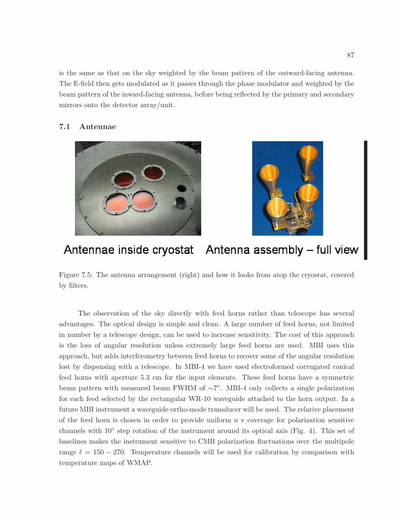
87
is the same as that on the sky weighted by the beam pattern of the outward-facing antenna.
The E-field then gets modulated as it passes through the phase modulator and weighted by the
beam pattern of the inward-facing antenna, before being reflected by the primary and secondary
mirrors onto the detector array/unit.
7.1 Antennae
Figure 7.5: The antenna arrangement (right) and how it looks from atop the cryostat, covered
by filters.
The observation of the sky directly with feed horns rather than telescope has several
advantages. The optical design is simple and clean. A large number of feed horns, not limited
in number by a telescope design, can be used to increase sensitivity. The cost of this approach
is the loss of angular resolution unless extremely large feed horns are used. MBI uses this
approach, but adds interferometry between feed horns to recover some of the angular resolution
lost by dispensing with a telescope. In MBI-4 we have used electroformed corrugated conical
feed horns with aperture 5.3 cm for the input elements. These feed horns have a symmetric
beam pattern with measured beam FWHM of ∼7. MBI-4 only collects a single polarization
for each feed selected by the rectangular WR-10 waveguide attached to the horn output. In a
future MBI instrument a waveguide ortho-mode transducer will be used. The relative placement
of the feed horn is chosen in order to provide uniform u v coverage for polarization sensitive
channels with 10 step rotation of the instrument around its optical axis (Fig. 4). This set of
baselines makes the instrument sensitive to CMB polarization fluctuations over the multipole
range ℓ = 150 − 270. Temperature channels will be used for calibration by comparison with
temperature maps of WMAP.
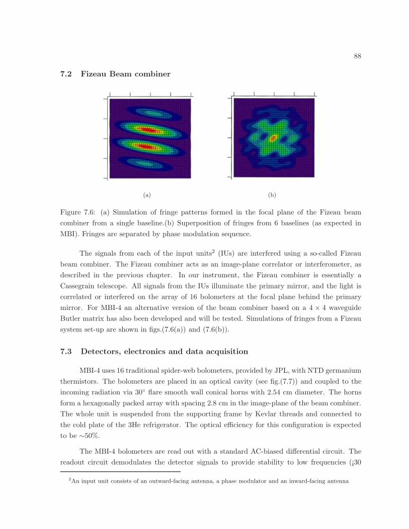
88
7.2 Fizeau Beam combiner
(a) (b)
Figure 7.6: (a) Simulation of fringe patterns formed in the focal plane of the Fizeau beam
combiner from a single baseline.(b) Superposition of fringes from 6 baselines (as expected in
MBI). Fringes are separated by phase modulation sequence.
The signals from each of the input units2 (IUs) are interfered using a so-called Fizeau
beam combiner. The Fizeau combiner acts as an image-plane correlator or interferometer, as
described in the previous chapter. In our instrument, the Fizeau combiner is essentially a
Cassegrain telescope. All signals from the IUs illuminate the primary mirror, and the light is
correlated or interfered on the array of 16 bolometers at the focal plane behind the primary
mirror. For MBI-4 an alternative version of the beam combiner based on a 4 × 4 waveguide
Butler matrix has also been developed and will be tested. Simulations of fringes from a Fizeau
system set-up are shown in figs.(7.6(a)) and (7.6(b)).
7.3 Detectors, electronics and data acquisition
MBI-4 uses 16 traditional spider-web bolometers, provided by JPL, with NTD germanium
thermistors. The bolometers are placed in an optical cavity (see fig.(7.7)) and coupled to the
incoming radiation via 30 flare smooth wall conical horns with 2.54 cm diameter. The horns
form a hexagonally packed array with spacing 2.8 cm in the image-plane of the beam combiner.
The whole unit is suspended from the supporting frame by Kevlar threads and connected to
the cold plate of the 3He refrigerator. The optical efficiency for this configuration is expected
to be ∼50%.
The MBI-4 bolometers are read out with a standard AC-biased differential circuit. The
readout circuit demodulates the detector signals to provide stability to low frequencies (¡30
2An input unit consists of an outward-facing antenna, a phase modulator and an inward-facing antenna
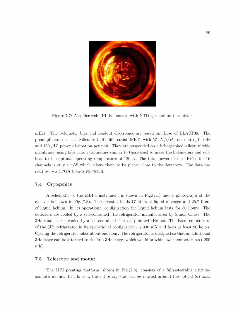
89
Figure 7.7: A spider-web JPL bolometer, with NTD germanium thermistor.
mHz). The bolometer bias and readout electronics are based on those of BLAST38. The
preamplifiers consist of Siliconix U401 differential JFETs with 57 nV/√Hz noise at ν¿100 Hz
and 120 µW power dissipation per pair. They are suspended on a lithographed silicon nitride
membrane, using fabrication techniques similar to those used to make the bolometers and self-
heat to the optimal operating temperature of 120 K. The total power of the JFETs for 16
channels is only 4 mW which allows them to be placed close to the detectors. The data are
read by two FPGA boards NI-7833R.
7.4 Cryogenics
A schematic of the MBI-4 instrument is shown in Fig.(7.1) and a photograph of the
receiver is shown in Fig.(7.3). The cryostat holds 17 liters of liquid nitrogen and 25.7 liters
of liquid helium. In its operational configuration the liquid helium lasts for 50 hours. The
detectors are cooled by a self-contained 3He refrigerator manufactured by Simon Chase. The
3He condenser is cooled by a self-contained charcoal-pumped 4He pot. The base temperature
of the 3He refrigerator in its operational configuration is 330 mK and lasts at least 90 hours.
Cycling the refrigerator takes about one hour. The refrigerator is designed so that an additional
3He stage can be attached to the first 3He stage, which would provide lower temperatures ( 200
mK).
7.5 Telescope and mount
The MBI pointing platform, shown in Fig.(7.8), consists of a fully-steerable altitude-
azimuth mount. In addition, the entire cryostat can be rotated around the optical (θ) axis.
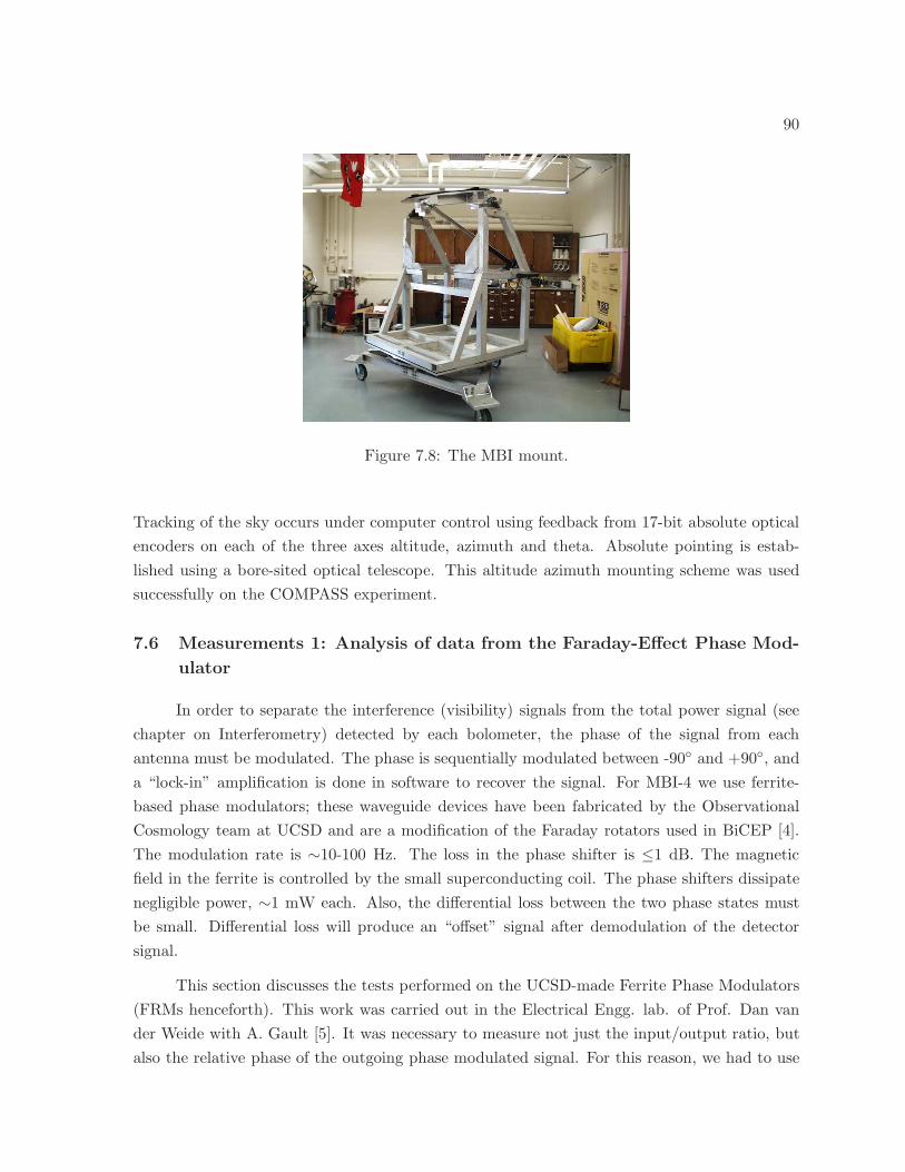
90
Figure 7.8: The MBI mount.
Tracking of the sky occurs under computer control using feedback from 17-bit absolute optical
encoders on each of the three axes altitude, azimuth and theta. Absolute pointing is estab-
lished using a bore-sited optical telescope. This altitude azimuth mounting scheme was used
successfully on the COMPASS experiment.
7.6 Measurements 1: Analysis of data from the Faraday-Effect Phase Mod-
ulator
In order to separate the interference (visibility) signals from the total power signal (see
chapter on Interferometry) detected by each bolometer, the phase of the signal from each
antenna must be modulated. The phase is sequentially modulated between -90 and +90, and
a “lock-in” amplification is done in software to recover the signal. For MBI-4 we use ferrite-
based phase modulators; these waveguide devices have been fabricated by the Observational
Cosmology team at UCSD and are a modification of the Faraday rotators used in BiCEP [4].
The modulation rate is ∼10-100 Hz. The loss in the phase shifter is ≤1 dB. The magnetic
field in the ferrite is controlled by the small superconducting coil. The phase shifters dissipate
negligible power, ∼1 mW each. Also, the differential loss between the two phase states must
be small. Differential loss will produce an “offset” signal after demodulation of the detector
signal.
This section discusses the tests performed on the UCSD-made Ferrite Phase Modulators
(FRMs henceforth). This work was carried out in the Electrical Engg. lab. of Prof. Dan van
der Weide with A. Gault [5]. It was necessary to measure not just the input/output ratio, but
also the relative phase of the outgoing phase modulated signal. For this reason, we had to use
91
a device that can not only generate an input signal for the FRM and measure the output/input
ratio (S21 henceforth (Appendix B) but also measure the relative phase of the outgoing signal.
This device is called a Vector Network Analyzer (VNA henceforth) because it can measure the
vector (i.e. both magnitude and phase) of outgoing signal values. Fig.(7.6) shows an early test
of one of the FRMs in MBI. The FRM is inside the cryostst.
7.6.1 Estimation - no losses
Let us suppose that we have a perfect measuring device; in particular, a perfect VNA.
In this case, the only reason where loss can occur is because the phase shift is not 90. This
is illustrated in fig.(7.10). Looking at fig.(7.10), we see that the fraction of the signal (in terms
of electric fields) that gets through is sin θ where θ is the amount of phase shift/rotation angle.
However, the VNA measures the power ratio, so that the ratio of input and output powers is
OutputPower
InputPower= sin2 θ (7.1)
However, this ratio is expressed in dB’s by the device where
S21 (dB) = 10 log10
(OutputPower
InputPower
)
= 10 log10
(sin2 θ
)≡ 20 log10 (sin θ) (7.2)
where
S21 (dB) = 10 log10 (S21 (ratio)) (7.3)
Then, the rotation angle can be extracted from S21 by the formula
θ = sin−1(
10S2120
)
(7.4)
7.6.2 Estimation with losses
If, however, there are losses in other parts of the set-up, e.g. waveguides, then S21 is no
longer a measure of the angle. We need to subtract this loss (the loss being represented by a
negative number in dBs) from S21, and then that quantity will be the true measure of rotation
angle.
The losses that we expect are as follows
1. Adapter losses
2. Waveguide losses
3. Ferrite losses
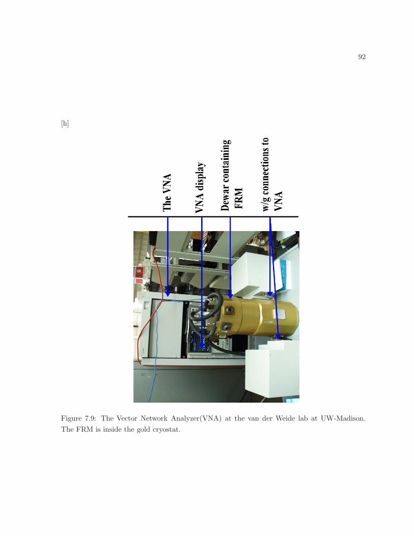
92
[h]
Figure 7.9: The Vector Network Analyzer(VNA) at the van der Weide lab at UW-Madison.
The FRM is inside the gold cryostat.
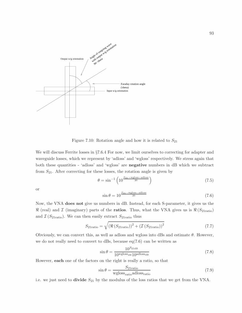
93
Output w/g orientation
Faraday rotation angle (\theta)
Angle of outgoing w
ave
with output w
/g orientatio
n
90−\theta
Input w/g orientation
Figure 7.10: Rotation angle and how it is related to S21
We will discuss Ferrite losses in §7.6.4 For now, we limit ourselves to correcting for adapter and
waveguide losses, which we represent by ‘adloss’ and ‘wgloss’ respectively. We stress again that
both these quantities - ‘adloss’ and ‘wgloss’ are negative numbers in dB which we subtract
from S21. After correcting for these losses, the rotation angle is given by
θ = sin−1(
10S21−wgloss−adloss
20
)
(7.5)
or
sin θ = 10S21−wgloss−adloss
20 (7.6)
Now, the VNA does not give us numbers in dB. Instead, for each S-parameter, it gives us the
ℜ (real) and I (imaginary) parts of the ratios. Thus, what the VNA gives us is ℜ (S21ratio)
and I (S21ratio). We can then easily extract S21ratio thus
S21ratio =
√
(ℜ (S21ratio))2 + (I (S21ratio))
2 (7.7)
Obviously, we can convert this, as well as adloss and wgloss into dBs and estimate θ. However,
we do not really need to convert to dBs, because eq(7.6) can be written as
sin θ =10S21dB
10wglossdB10adlossdB(7.8)
However, each one of the factors on the right is really a ratio, so that
sin θ =S21ratio
wglossratioadlossratio(7.9)
i.e. we just need to divide S21 by the modulus of the loss ratios that we get from the VNA.
94
7.6.3 Correcting for Ferrite loss
In principle, we need to correct for ferrite loss in exactly the same way, i.e.
sin θ =S21ratio
wglossratioadlossratioflossratio(7.10)
where ‘flossratio’ is the ferrite loss as a ratio. However, it cannot be measured in any obvious
way unlike adloss and wgloss, which are measured by an adapter calibration and a separate
baseline test respectively. Instead, we need to make an estimate indirectly as follows
1. From the ferrite-uncorrected angle vs. current graph, find a current for which the rotation
angle is zero
2. Find the S11 for this current, as a ratio
3. This S11 is the result of the wave traversing the entire length of waveguide once, plus
traversing through the ferrite twice (after correcting for adapter loss).
4. Subtract wgloss obtained from the baseline test from this S11
After the aforementioned operations are done, this S11 is a good estimate of twice the ferrite
loss (in dB) ≡ square of the ferrite loss ratio (as a ratio). Now, we are ready to obtain the
corrected θ:
sin θ =S21ratio
wglossratioadlossratioflossratio (corrected)(7.11)
This is what was done, and the result is in fig.(7.11).
7.6.4 Over/under-estimation of Ferrite loss
If we pick out the current at which the phase shift angle is zero, and if S11 and S22 are
the same, then loss estimation is exact. However, this is rarely ever the case. In reality, the
current chosen always has some non-zero phase-shift associated with it. If so, we have actually
underestimated the loss in the ferrite. Then there is the question of whether the hysteresis
loop is symmetric.
To summarize, the estimation error could be a combination of the following factors:
1. Asymmetry in the reflection at the zero-phase angle point
2. The supposed “zero-phase angle” point not being at exactly zero angle
3. The asymmetry of the hysteresis loop because of other reasons
95
The following possibilities exist about point 2 above:
1. If θ is the phase angle at the current we have chosen, S11 is off by a factor of sin θ, so that
we need a corrective multiplicative factor of 11−sin θ
2. The factor in point (1) above is actually sin2 θ instead of sin θ, so the corrective factor is1
1−sin2 θ≡ 1
cos2 θ
3. The factor is 1cos θ
This will be discussed in greater detail in[5]. Concerning points 1 and 3 above, an iterative
approach is a good solution in the absence of a detailed knowledge of the modulator. In this
iterative scheme, we shift the hysteresis loop in every iteration until it is approximately centered
and then recalculate all parameters. We can continue to repeat these steps until the required
accuracy is reached.
7.7 Measurements 2: Antenna Beam Patterns
Since MBI is ground-based, it has to detect sub-µK signals in the vicinity of warm sources
(the Earth, the sky). This level of accuracy has never been studied before in any ground-based
telescope system. We need an excellent understanding of the beam pattern of MBI for the
following reasons.
1. Hu et al. [6] have shown that even if the errors in the main beam are very low, the
corresponding error in measuring polarization is huge, because the temperature signal,
which is 2-3 orders of magnitude higher than polarization for the CMB, “leaks” into the
polarization signal, and even a small leakage causes huge errors in observed polarization,
and changes one form of polarization into another (true especially of sidelobes, however
low). This makes it extremely difficult to extract useful cosmological information from
the data.
2. Antenna sidelobes can couple signals from warm objects (the sky, the Earth).
These are problems that will challenge the next generation CMB polarization probes. For this
reason, antenna beam patterns need to be measured to exquisite precision in order to eliminate
mixing the CMB temperature signal into polarization (to ∼1 part in 108).
Requirements of beam-mapping measurement:
The top of the MBI instrument is about 3 m above the ground and the antennae receive
signals in a band of a wavelengths centered on 3mm. All cosmological sources are at a distance
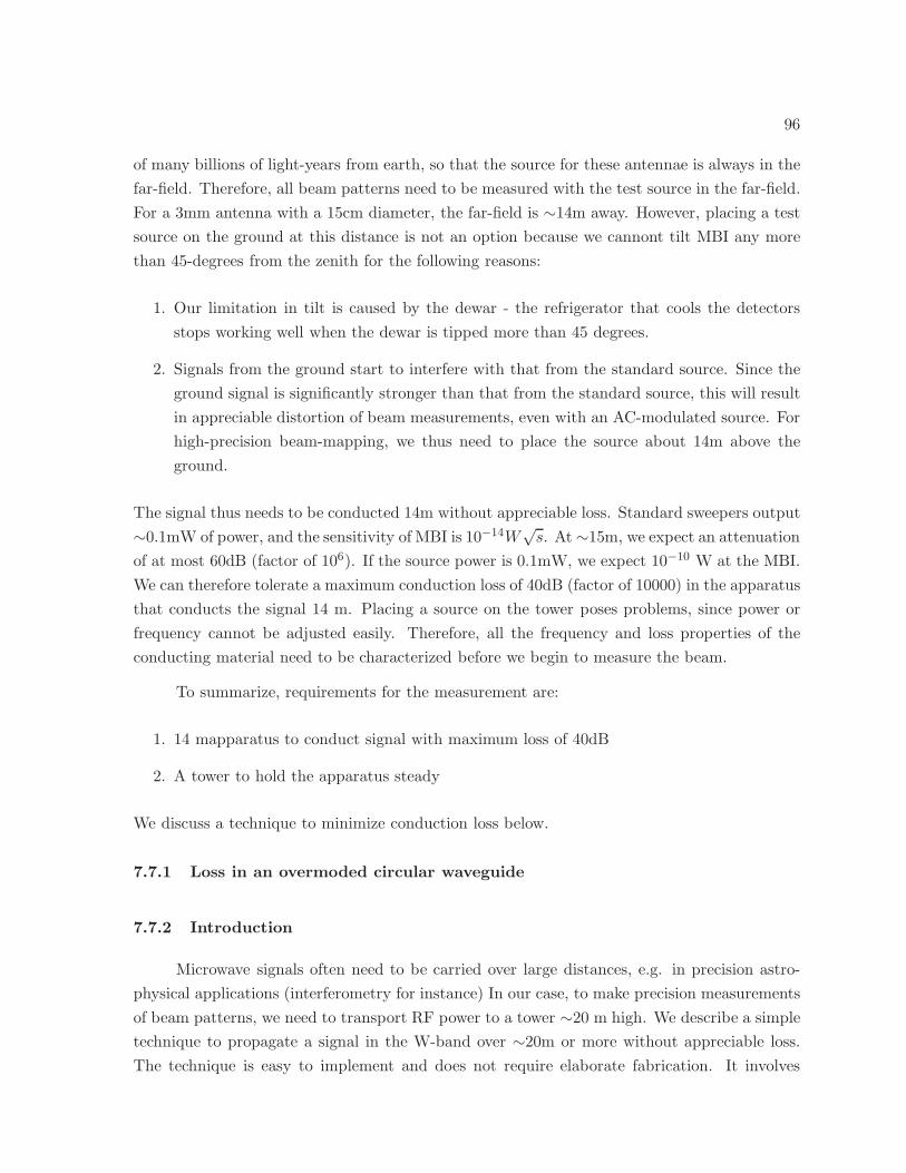
96
of many billions of light-years from earth, so that the source for these antennae is always in the
far-field. Therefore, all beam patterns need to be measured with the test source in the far-field.
For a 3mm antenna with a 15cm diameter, the far-field is ∼14m away. However, placing a test
source on the ground at this distance is not an option because we cannont tilt MBI any more
than 45-degrees from the zenith for the following reasons:
1. Our limitation in tilt is caused by the dewar - the refrigerator that cools the detectors
stops working well when the dewar is tipped more than 45 degrees.
2. Signals from the ground start to interfere with that from the standard source. Since the
ground signal is significantly stronger than that from the standard source, this will result
in appreciable distortion of beam measurements, even with an AC-modulated source. For
high-precision beam-mapping, we thus need to place the source about 14m above the
ground.
The signal thus needs to be conducted 14m without appreciable loss. Standard sweepers output
∼0.1mW of power, and the sensitivity of MBI is 10−14W√s. At ∼15m, we expect an attenuation
of at most 60dB (factor of 106). If the source power is 0.1mW, we expect 10−10 W at the MBI.
We can therefore tolerate a maximum conduction loss of 40dB (factor of 10000) in the apparatus
that conducts the signal 14 m. Placing a source on the tower poses problems, since power or
frequency cannot be adjusted easily. Therefore, all the frequency and loss properties of the
conducting material need to be characterized before we begin to measure the beam.
To summarize, requirements for the measurement are:
1. 14 mapparatus to conduct signal with maximum loss of 40dB
2. A tower to hold the apparatus steady
We discuss a technique to minimize conduction loss below.
7.7.1 Loss in an overmoded circular waveguide
7.7.2 Introduction
Microwave signals often need to be carried over large distances, e.g. in precision astro-
physical applications (interferometry for instance) In our case, to make precision measurements
of beam patterns, we need to transport RF power to a tower ∼20 m high. We describe a simple
technique to propagate a signal in the W-band over ∼20m or more without appreciable loss.
The technique is easy to implement and does not require elaborate fabrication. It involves
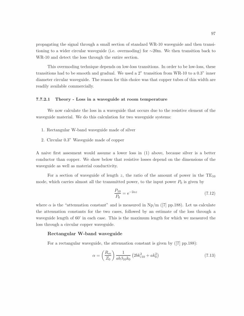
97
propagating the signal through a small section of standard WR-10 waveguide and then transi-
tioning to a wider circular waveguide (i.e. overmoding) for ∼20m. We then transition back to
WR-10 and detect the loss through the entire section.
This overmoding technique depends on low-loss transitions. In order to be low-loss, these
transitions had to be smooth and gradual. We used a 2” transition from WR-10 to a 0.3” inner
diameter circular waveguide. The reason for this choice was that copper tubes of this width are
readily available commercially.
7.7.2.1 Theory - Loss in a waveguide at room temperature
We now calculate the loss in a waveguide that occurs due to the resistive element of the
waveguide material. We do this calculation for two waveguide systems:
1. Rectangular W-band waveguide made of silver
2. Circular 0.3” Waveguide made of copper
A naive first assesment would assume a lower loss in (1) above, because silver is a better
conductor than copper. We show below that resistive losses depend on the dimensions of the
waveguide as well as material conductivity.
For a section of waveguide of length z, the ratio of the amount of power in the TE10
mode, which carries almost all the transmitted power, to the input power P0 is given by
P10
P0= e−2αz (7.12)
where α is the “attenuation constant” and is measured in Np/m ([7] pp.188). Let us calculate
the attenuation constants for the two cases, followed by an estimate of the loss through a
waveguide length of 60’ in each case. This is the maximum length for which we measured the
loss through a circular copper waveguide.
Rectangular W-band waveguide
For a rectangular waveguide, the attenuation constant is given by ([7] pp.188):
α =
(RmZ0
)1
abβ10k0
(2bk2
c10 + ak20
)(7.13)
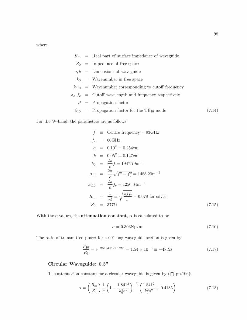
98
where
Rm = Real part of surface impedance of waveguide
Z0 = Impedance of free space
a, b = Dimensions of waveguide
k0 = Wavenumber in free space
kc10 = Wavenumber corresponding to cutoff frequency
λc, fc = Cutoff wavelength and frequency respectively
β = Propagation factor
β10 = Propagation factor for the TE10 mode (7.14)
For the W-band, the parameters are as follows:
f ≡ Centre frequency = 93GHz
fc = 60GHz
a = 0.10′′ ≡ 0.254cm
b = 0.05′′ ≡ 0.127cm
k0 =2π
cf = 1947.79m−1
β10 =2π
c
√
f2 − f2c = 1488.20m−1
kc10 =2π
cfc = 1256.64m−1
Rm =1
σδ≡√
πfµ
σ= 0.078 for silver
Z0 = 377Ω (7.15)
With these values, the attenuation constant, α is calculated to be
α = 0.303Np/m (7.16)
The ratio of transmitted power for a 60’-long waveguide section is given by
P10
P0= e−2×0.303×18.288 = 1.54× 10⁻⁵ ≡ −48dB (7.17)
Circular Waveguide: 0.3”
The attenuation constant for a circular waveguide is given by ([7] pp.196):
α =
(RmZ0
)1
a
(
1− 1.8412
k20a
2
)− 12(
1.8412
k20a
2+ 0.4185
)
(7.18)
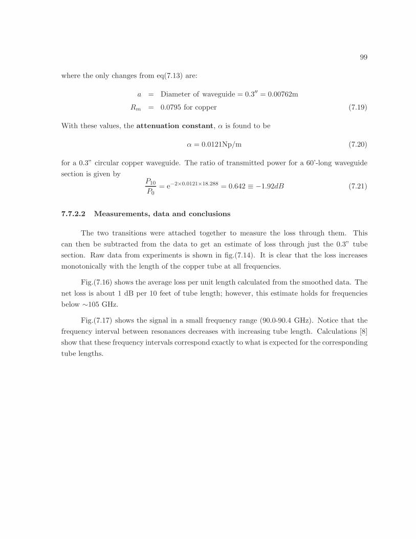
99
where the only changes from eq(7.13) are:
a = Diameter of waveguide = 0.3′′ = 0.00762m
Rm = 0.0795 for copper (7.19)
With these values, the attenuation constant, α is found to be
α = 0.0121Np/m (7.20)
for a 0.3” circular copper waveguide. The ratio of transmitted power for a 60’-long waveguide
section is given byP10
P0= e−2×0.0121×18.288 = 0.642 ≡ −1.92dB (7.21)
7.7.2.2 Measurements, data and conclusions
The two transitions were attached together to measure the loss through them. This
can then be subtracted from the data to get an estimate of loss through just the 0.3” tube
section. Raw data from experiments is shown in fig.(7.14). It is clear that the loss increases
monotonically with the length of the copper tube at all frequencies.
Fig.(7.16) shows the average loss per unit length calculated from the smoothed data. The
net loss is about 1 dB per 10 feet of tube length; however, this estimate holds for frequencies
below ∼105 GHz.
Fig.(7.17) shows the signal in a small frequency range (90.0-90.4 GHz). Notice that the
frequency interval between resonances decreases with increasing tube length. Calculations [8]
show that these frequency intervals correspond exactly to what is expected for the corresponding
tube lengths.
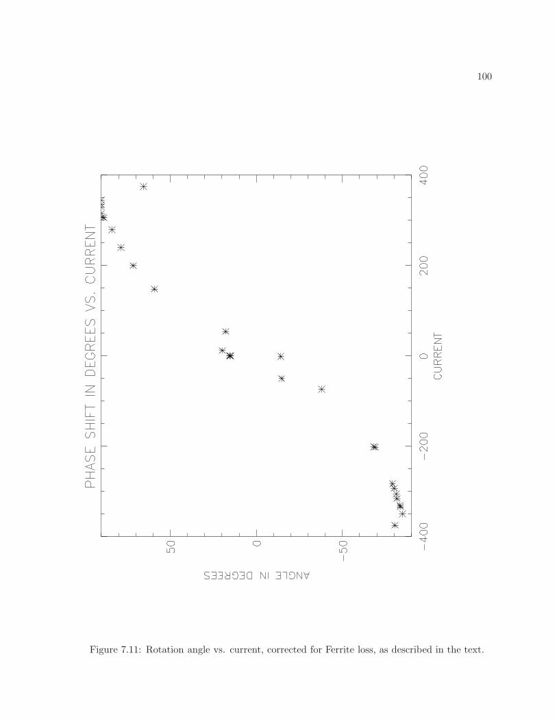
100
Figure 7.11: Rotation angle vs. current, corrected for Ferrite loss, as described in the text.
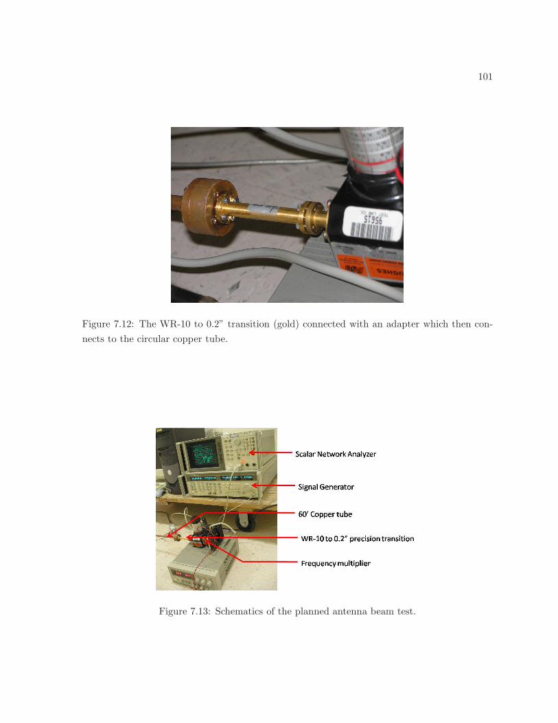
101
Figure 7.12: The WR-10 to 0.2” transition (gold) connected with an adapter which then con-
nects to the circular copper tube.
Figure 7.13: Schematics of the planned antenna beam test.
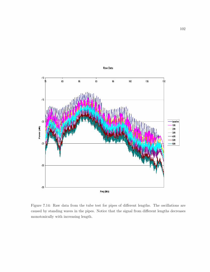
102
Figure 7.14: Raw data from the tube test for pipes of different lengths. The oscillations are
caused by standing waves in the pipes. Notice that the signal from different lengths decreases
monotonically with increasing length.
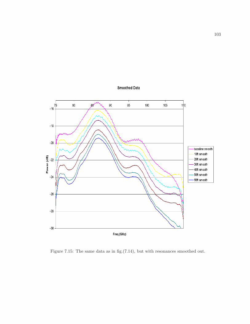
103
Figure 7.15: The same data as in fig.(7.14), but with resonances smoothed out.
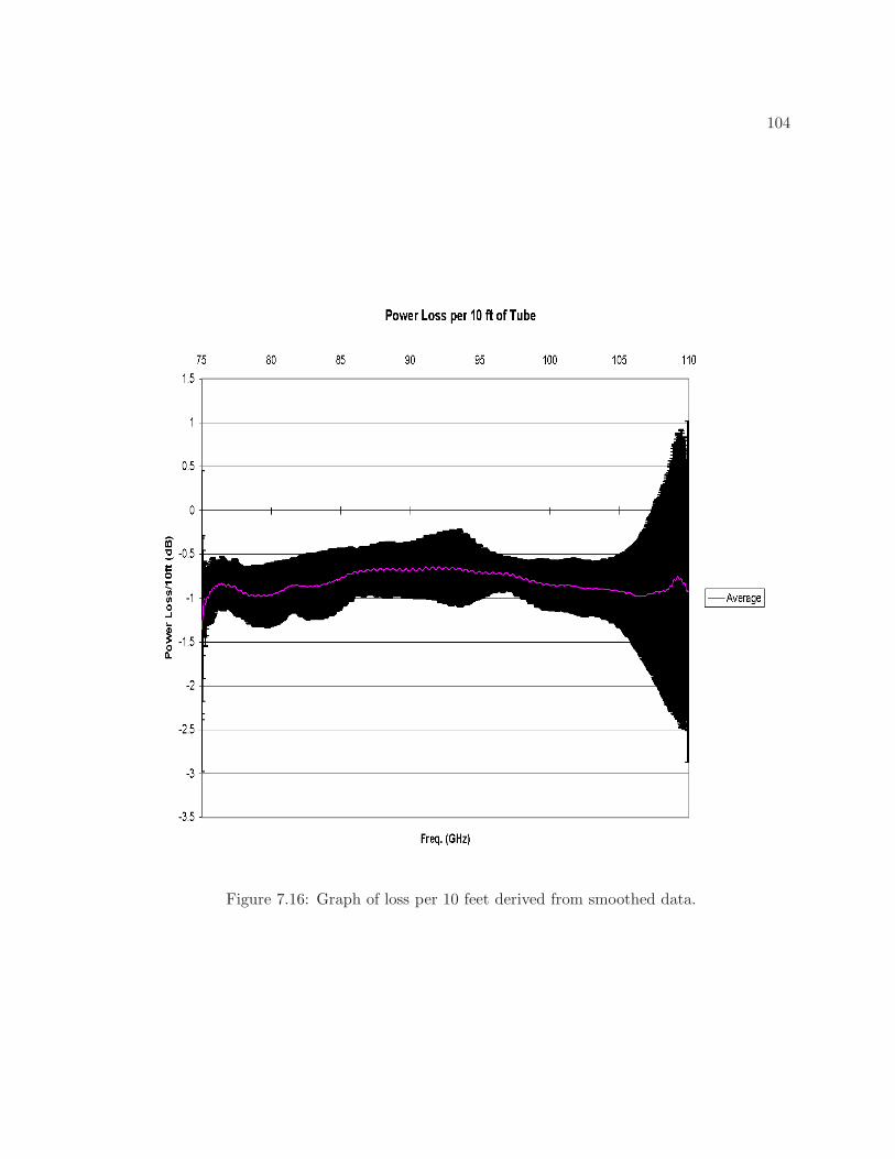
104
Figure 7.16: Graph of loss per 10 feet derived from smoothed data.
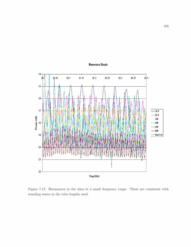
105
Figure 7.17: Resonances in the data in a small frequency range. These are consistent with
standing waves in the tube lengths used.
106
Bibliography
[1] P. T. Timbie, G. S. Tucker, P. A. R. Ade, S. Ali, E. Bierman, E. F. Bunn, C. Calderon,
A. C. Gault, P. O. Hyland, B. G. Keating, J. Kim, A. Korotkov, S. S. Malu, P. Mauskopf,
J. A. Murphy, C. O’Sullivan, L. Piccirillo, and B. D. Wandelt, “The Einstein polarization
interferometer for cosmology (EPIC) and the millimeter-wave bolometric interferometer
(MBI),” New Astronomy Review, vol. 50, pp. 999–1008, Dec. 2006.
[2] C. L. Bennett, R. S. Hill, G. Hinshaw, M. R. Nolta, N. Odegard, L. Page, D. N. Spergel,
J. L. Weiland, E. L. Wright, M. Halpern, N. Jarosik, A. Kogut, M. Limon, S. S. Meyer,
G. S. Tucker, and E. Wollack, “First-Year Wilkinson Microwave Anisotropy Probe (WMAP)
Observations: Foreground Emission,” ApJ Suppl., vol. 148, pp. 97–117, Sept. 2003.
[3] J. Bock, S. Church, M. Devlin, G. Hinshaw, A. Lange, A. Lee, L. Page, B. Partridge,
J. Ruhl, M. Tegmark, P. Timbie, R. Weiss, B. Winstein, and M. Zaldarriaga, “Task Force
on Cosmic Microwave Background Research,” ArXiv Astrophysics e-prints, Apr. 2006.
[4] K. W. Yoon, P. A. Ade, D. Barkats, J. O. Battle, E. M. Bierman, J. J. Bock, H. C. Chiang,
C. D. Dowell, L. Duband, G. S. Griffin, E. F. Hivon, W. L. Holzapfel, V. V. Hristov, B. G.
Keating, J. M. Kovac, C. Kuo, A. E. Lange, E. M. Leitch, P. V. Mason, H. T. Nguyen,
N. Ponthieu, and Y. D. Takahashi, “Report on BICEP’s First Season Observing the Cosmic
Microwave Background from South Pole,” in Bulletin of the American Astronomical Society,
Dec. 2006, vol. 38 of Bulletin of the American Astronomical Society, pp. 963–+.
[5] A. C. Gault and S. S. Malu, “A measurement of the Faraday-effect Phase modulator
performance,” In preparation, 2007.
[6] W. Hu, M. M. Hedman, and M. Zaldarriaga, “Benchmark parameters for CMB polarization
experiments,” Phys. Rev. D, vol. 67, no. 4, pp. 043004–+, Feb. 2003.
[7] R. E. Collin, Foundations for Microwave Engineering, Wiley-IEEE Press. ISBN-13 978-
0780360310, 2000, XIII + 944 p. 2nd ed., 2000.
[8] L. Levac, S. S. Malu, and P. T. Timbie, “Loss in an overmoded circular waveguide over
medium distances,” In preparation, 2007.
107
Chapter 8
Simulations of the CMB sky and the MBI
Instrument
In chapter 7, we described the MBI instrument in detail. Before the MBI can be put to use in
CMB observations, though, we need to know:
1. its response to a simulated CMB sky, in order to perform checks on its various parts
2. its response as a function of ℓ, which depends on its antenna beams patterns.
To achieve this, we need the following calculations/simulations:
1. simulation of the CMB sky over a patch as large as the MBI beam
2. a calculation of the Window functions of MBI for CXℓ where X = T,E,B
3. simulation of the MBI instrument
In addition, we need to describe the analysis of data from the FRM.
We describe these three calculations/simulations below.
8.1 Simulation of the CMB sky patch
As described in §5.6, the power spectrum is a statistical description of CMB anisotropies.
That is, it does not contain information about the amount of power in every single anisotropy
over the sky as a function of position. Instead, it tells us how much power there is in the
anisotropy at a given angular scale. This can be pictured as follows. Imagine a point on the
sky, say θ = 0, i.e. the NCP. Now consider all the points (ideally, infinite, but practically, a
large number) at some θ 6= 0. If we compare the temperature at θ = 0 with the temperatures
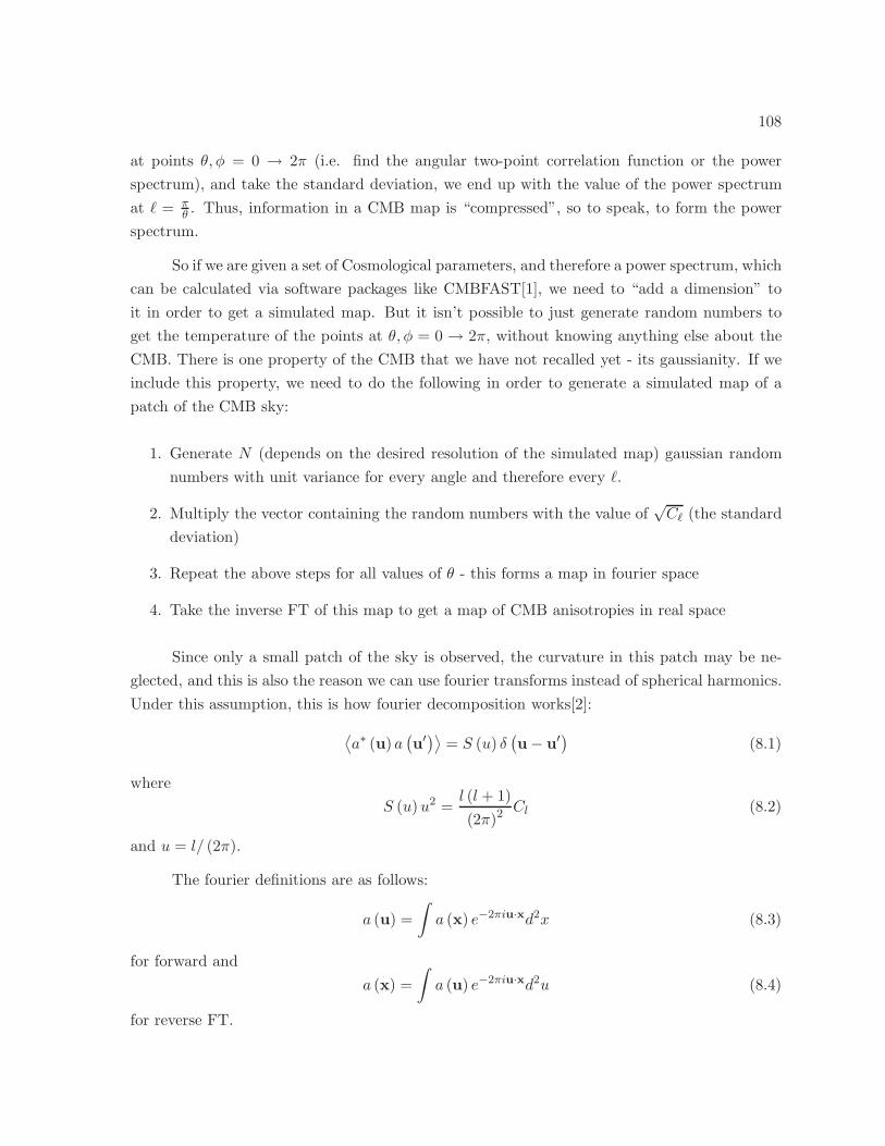
108
at points θ, φ = 0 → 2π (i.e. find the angular two-point correlation function or the power
spectrum), and take the standard deviation, we end up with the value of the power spectrum
at ℓ = πθ . Thus, information in a CMB map is “compressed”, so to speak, to form the power
spectrum.
So if we are given a set of Cosmological parameters, and therefore a power spectrum, which
can be calculated via software packages like CMBFAST[1], we need to “add a dimension” to
it in order to get a simulated map. But it isn’t possible to just generate random numbers to
get the temperature of the points at θ, φ = 0 → 2π, without knowing anything else about the
CMB. There is one property of the CMB that we have not recalled yet - its gaussianity. If we
include this property, we need to do the following in order to generate a simulated map of a
patch of the CMB sky:
1. Generate N (depends on the desired resolution of the simulated map) gaussian random
numbers with unit variance for every angle and therefore every ℓ.
2. Multiply the vector containing the random numbers with the value of√Cℓ (the standard
deviation)
3. Repeat the above steps for all values of θ - this forms a map in fourier space
4. Take the inverse FT of this map to get a map of CMB anisotropies in real space
Since only a small patch of the sky is observed, the curvature in this patch may be ne-
glected, and this is also the reason we can use fourier transforms instead of spherical harmonics.
Under this assumption, this is how fourier decomposition works[2]:
⟨a∗ (u) a
(u′)⟩ = S (u) δ
(u− u′) (8.1)
where
S (u)u2 =l (l + 1)
(2π)2Cl (8.2)
and u = l/ (2π).
The fourier definitions are as follows:
a (u) =
∫
a (x) e−2πiu·xd2x (8.3)
for forward and
a (x) =
∫
a (u) e−2πiu·xd2u (8.4)
for reverse FT.
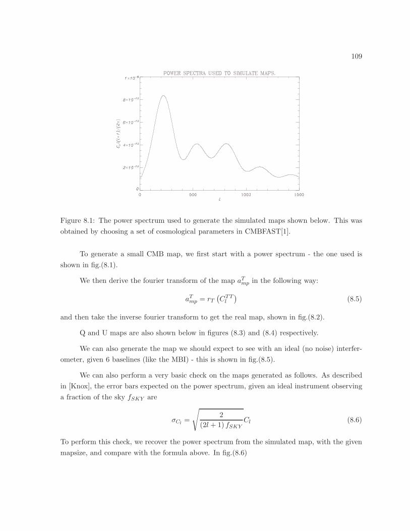
109
Figure 8.1: The power spectrum used to generate the simulated maps shown below. This was
obtained by choosing a set of cosmological parameters in CMBFAST[1].
To generate a small CMB map, we first start with a power spectrum - the one used is
shown in fig.(8.1).
We then derive the fourier transform of the map aTmp in the following way:
aTmp = rT(CTTl
)(8.5)
and then take the inverse fourier transform to get the real map, shown in fig.(8.2).
Q and U maps are also shown below in figures (8.3) and (8.4) respectively.
We can also generate the map we should expect to see with an ideal (no noise) interfer-
ometer, given 6 baselines (like the MBI) - this is shown in fig.(8.5).
We can also perform a very basic check on the maps generated as follows. As described
in [Knox], the error bars expected on the power spectrum, given an ideal instrument observing
a fraction of the sky fSKY are
σCl=
√
2
(2l + 1) fSKYCl (8.6)
To perform this check, we recover the power spectrum from the simulated map, with the given
mapsize, and compare with the formula above. In fig.(8.6)
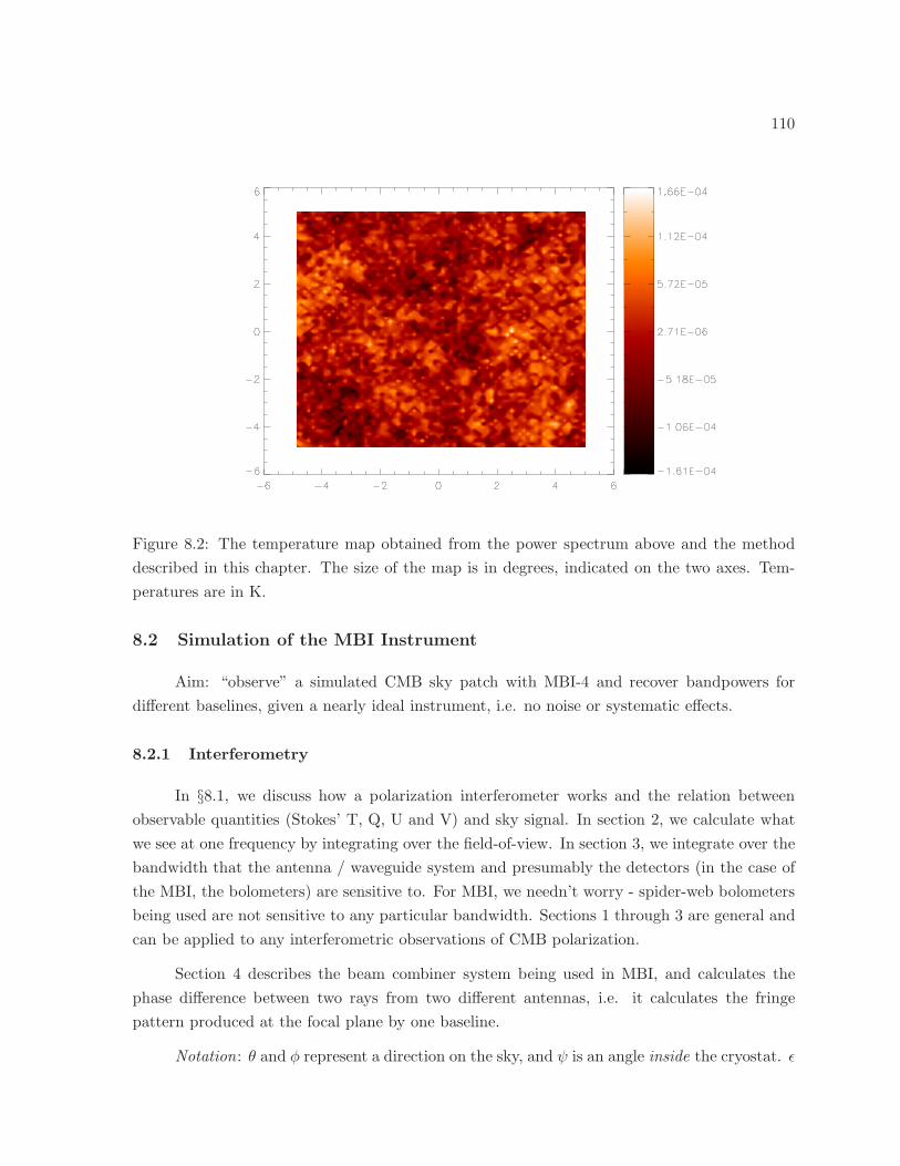
110
Figure 8.2: The temperature map obtained from the power spectrum above and the method
described in this chapter. The size of the map is in degrees, indicated on the two axes. Tem-
peratures are in K.
8.2 Simulation of the MBI Instrument
Aim: “observe” a simulated CMB sky patch with MBI-4 and recover bandpowers for
different baselines, given a nearly ideal instrument, i.e. no noise or systematic effects.
8.2.1 Interferometry
In §8.1, we discuss how a polarization interferometer works and the relation between
observable quantities (Stokes’ T, Q, U and V) and sky signal. In section 2, we calculate what
we see at one frequency by integrating over the field-of-view. In section 3, we integrate over the
bandwidth that the antenna / waveguide system and presumably the detectors (in the case of
the MBI, the bolometers) are sensitive to. For MBI, we needn’t worry - spider-web bolometers
being used are not sensitive to any particular bandwidth. Sections 1 through 3 are general and
can be applied to any interferometric observations of CMB polarization.
Section 4 describes the beam combiner system being used in MBI, and calculates the
phase difference between two rays from two different antennas, i.e. it calculates the fringe
pattern produced at the focal plane by one baseline.
Notation: θ and φ represent a direction on the sky, and ψ is an angle inside the cryostat. ǫ
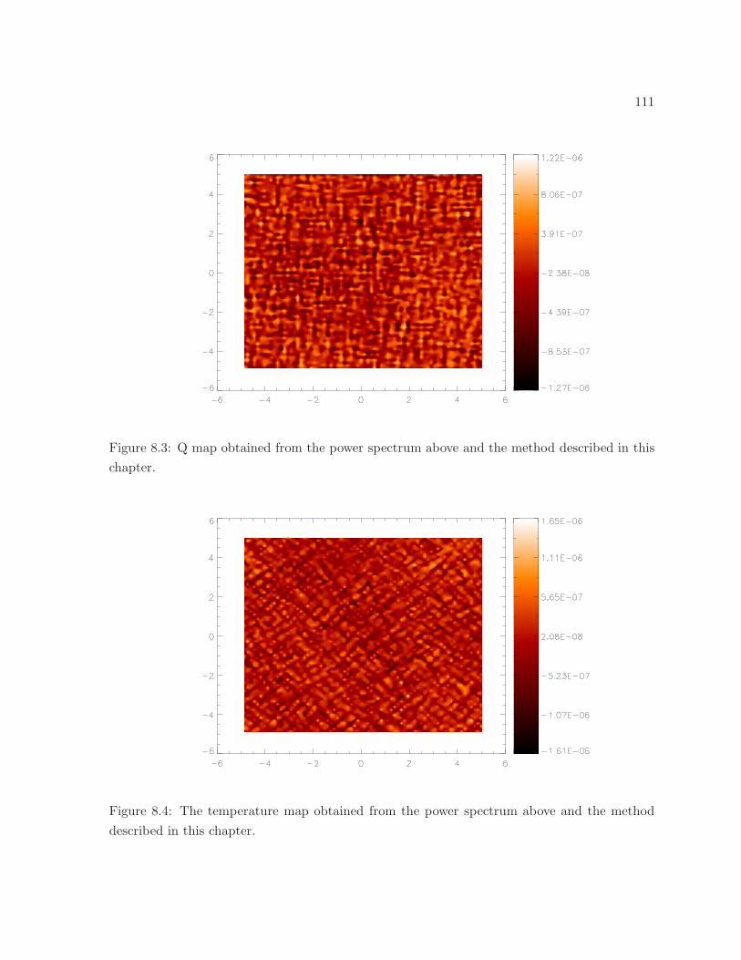
111
Figure 8.3: Q map obtained from the power spectrum above and the method described in this
chapter.
Figure 8.4: The temperature map obtained from the power spectrum above and the method
described in this chapter.
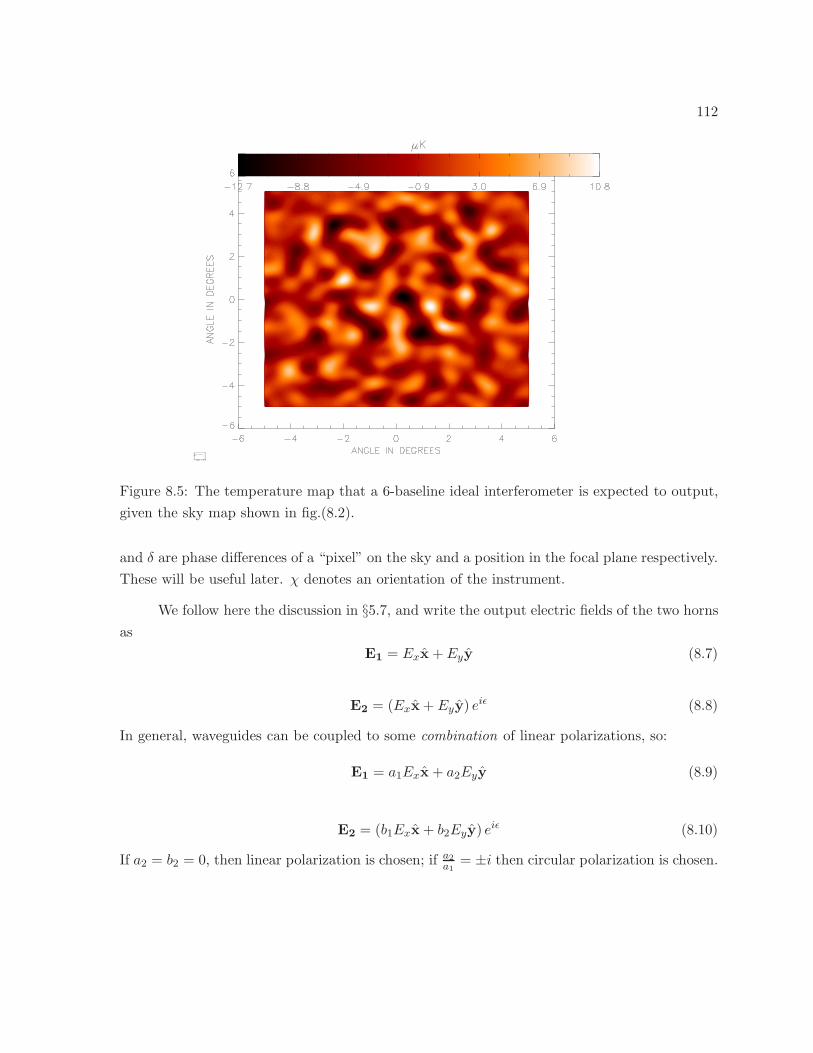
112
Figure 8.5: The temperature map that a 6-baseline ideal interferometer is expected to output,
given the sky map shown in fig.(8.2).
and δ are phase differences of a “pixel” on the sky and a position in the focal plane respectively.
These will be useful later. χ denotes an orientation of the instrument.
We follow here the discussion in §5.7, and write the output electric fields of the two horns
as
E1 = Exx +Eyy (8.7)
E2 = (Exx + Eyy) eiǫ (8.8)
In general, waveguides can be coupled to some combination of linear polarizations, so:
E1 = a1Exx + a2Eyy (8.9)
E2 = (b1Exx + b2Eyy) eiǫ (8.10)
If a2 = b2 = 0, then linear polarization is chosen; if a2a1 = ±i then circular polarization is chosen.
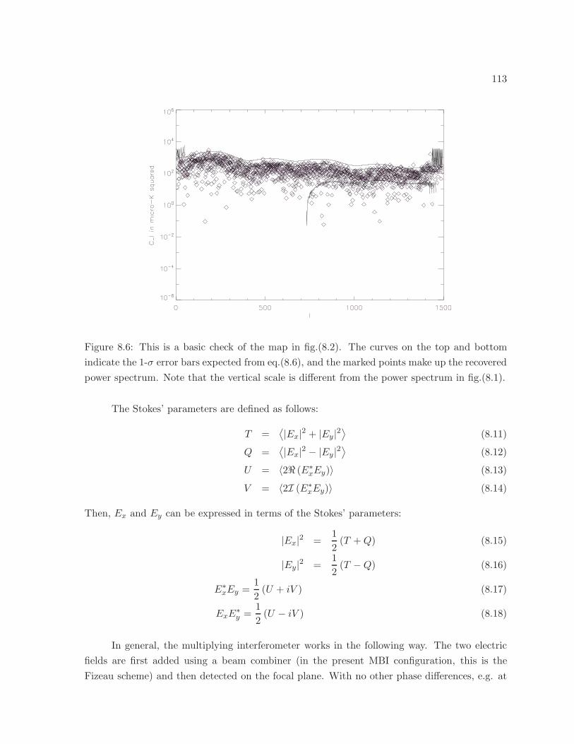
113
Figure 8.6: This is a basic check of the map in fig.(8.2). The curves on the top and bottom
indicate the 1-σ error bars expected from eq.(8.6), and the marked points make up the recovered
power spectrum. Note that the vertical scale is different from the power spectrum in fig.(8.1).
The Stokes’ parameters are defined as follows:
T =⟨|Ex|2 + |Ey|2
⟩(8.11)
Q =⟨|Ex|2 − |Ey|2
⟩(8.12)
U = 〈2ℜ (E∗xEy)〉 (8.13)
V = 〈2I (E∗xEy)〉 (8.14)
Then, Ex and Ey can be expressed in terms of the Stokes’ parameters:
|Ex|2 =1
2(T +Q) (8.15)
|Ey|2 =1
2(T −Q) (8.16)
E∗xEy =
1
2(U + iV ) (8.17)
ExE∗y =
1
2(U − iV ) (8.18)
In general, the multiplying interferometer works in the following way. The two electric
fields are first added using a beam combiner (in the present MBI configuration, this is the
Fizeau scheme) and then detected on the focal plane. With no other phase differences, e.g. at
114
exactly the middle of the focal plane the output at the detector will be (E1 + E2) (E∗1 + E∗
2).
However, there will be an additional phase factor due to the difference in path length between
the two paths to the focal plane from the two antennas, as shown in figure 1. There is a relative
phase of ǫ due to the position of the two antennas looking towards the sky and δ between the
rays from antenna two and antenna one inside the cryostat, and therefore between E1 and E2.
Now recall that the part of the detected signal that has been phase modulated is ∝ E1E∗2
and its conjugate. Let us work out the detected quantity explicitly:
(
E1 + E2ei(δ+ǫ)
)(
E∗1 + E∗
2e−i(δ+ǫ)
)
= |E1|2 + |E2|2 + E1E∗2e
−i(δ+ǫ) + E∗1E2e
i(δ+ǫ) (8.19)
The first two terms are easily evaluated:
|E1|2 = E1E∗1 = |a1|2|Ex|2 + |a2|2|Ey|2 (8.20)
|E2|2 = E2E∗2 = |b1|2|Ex|2 + |b2|2|Ey|2 (8.21)
We can substitute for |Ex|2 etc. from the above equations to get
|E1|2 =1
2
[T(|a2
1|+ |a22|)
+Q(|a2
1| − |a22|)]
(8.22)
|E2|2 =1
2
[T(|b21|+ |b22|
)+Q
(|b21| − |b22|
)](8.23)
If we want to study interference, we wish to look at only the last two terms, which will
have been phase-modulated. However, they are just complex conjugates of each other. So we
need evaluate only one, and the other will follow. WLOG, we consider the last term:
⟨
E∗1E2e
i(δ+ǫ)⟩
=1
2ei(δ+ǫ) [a∗1b1 (T +Q) + a2b
∗2 (T −Q) + a∗1b2 (U − iV ) + a∗2b1 (U + iV )]
(8.24)
Simplifying,
⟨
E∗1E2e
i(δ+ǫ)⟩
=1
2ei(δ+ǫ) ×
[(a∗1b1 + a∗2b2)T + (a∗1b1 − a∗2b2)Q+ (a∗1b2 + a∗2b1)U + i (a∗2b1 − a∗1b2)V ] (8.25)
Similarly,
⟨
E1E∗2e
−i(δ+ǫ)⟩
=1
2e−i(δ+ǫ) ×
[(a1b∗1 + a2b
∗2)T + (a1b
∗1 − a2b
∗2)Q+ (a1b
∗2 + a2b
∗1)U − i (a2b
∗1 − a1b
∗2)V ] (8.26)
We need to remind ourselves that the four quantities T,Q,U and V already have the effect of
the primary antenna beam included. Just so we are clear, let us replace T etc. by T where
115
T = A (φ, θ)T etc. thus:
⟨
E∗1E2e
iδ⟩
=1
2ei(δ−ǫ) [(a∗1b1 + a∗2b2)T + (a∗1b1 − a∗2b2)Q+ (a∗1b2 + a∗2b1)U + i (a∗2b1 − a∗1b2)V]
(8.27)
and
⟨
E1E∗2e
−iδ⟩
=1
2e−i(δ−ǫ) ×
[(a1b∗1 + a2b
∗2)T + (a1b
∗1 − a2b
∗2)Q+ (a1b
∗2 + a2b
∗1)U − i (a2b
∗1 − a1b
∗2)V] (8.28)
We need to assign one kind of polarization, i.e. either linear or circular, in order to figure
out the sum of these two quantities. Let us consider the case of linear polarization first, where
X ≡(a2=0a1=1
)and Y ≡
(a1=0a2=1
)for E1 and X ≡
(b2=0b1=1
)and Y ≡
(b1=0b2=1
)for E2, so that
⟨
E1E∗2e
−iδ⟩
XX=
1
2e−i(δ−ǫ) (T +Q) (8.29)
⟨
E1E∗2e
−iδ⟩
Y Y=
1
2e−i(δ−ǫ) (T − Q) (8.30)
⟨
E1E∗2e
−iδ⟩
XY=
1
2e−i(δ−ǫ) (U + iV) (8.31)
⟨
E1E∗2e
−iδ⟩
Y X=
1
2e−i(δ−ǫ) (U − iV) (8.32)
And similarly, the complex conjugate term gives us
⟨
E∗1E2e
iδ⟩
XX=
1
2ei(δ−ǫ) (T +Q) (8.33)
⟨
E∗1E2e
iδ⟩
Y Y=
1
2ei(δ−ǫ) (T − Q) (8.34)
⟨
E∗1E2e
iδ⟩
XY=
1
2ei(δ−ǫ) (U + iV) (8.35)
⟨
E∗1E2e
iδ⟩
Y X=
1
2ei(δ−ǫ) (U − iV) (8.36)
8.2.1.1 Application to simulations of time-ordered data (TOD)
In an interferometer, the only diference between the electric fields at the different antennas
is a phase factor that depends on the path difference between the photons that arrive at those
antennas. Therefore, we need to find the electric field at only one antenna; the field at the
others will follow easily.
Following equations 9 and 10, we get for the two components of the electric field:
|Ex|2 =1
2(T +Q) (8.37)
|Ey|2 =1
2(T − Q) (8.38)
116
It seems a little strange at first that the electric fields be maps instead of just a number, but
we have to remember that they do not get added/averaged over until they reach the detectors.
At the detector, they are summed over with all the appropriate phase factors.
8.2.2 Integration over the field-of-view (FOV) / sky patch
This is not a single step, since there are several things involved:
1. Q and U as functions of orientation χ: As the instrument is rotated, the response
from every baseline changes - Q and U are functions of orientation angle χ - this relation
is described in the appendix.
2. Relative phase of each point on the sky: Every antenna’s position is a point, and
the distance of every point in the sky patch / field-of-view to the antenna is different;
consequently, each point on the FOV has a unique phase associated with it, which needs
to be calculated. In other words, we need to calculate the exact functional form of ǫ,
which is a function of φ, θ and χ
Let us perform each operation, one by one. Before performing integration, though, we need to
get the units of each quantity right. The units of the incoming power are Wm−2Hz−1Sr−1.
8.2.2.1 Integration
We can simply integrate over an “area” on the sky. An “area” on the sky is given by
A =
∫ θ2
θ=θ1
∫ φ2
φ=φ1
sin θdφdθ (8.39)
where θ1 and φ1 can have any value depending on which part of the sky we are looking at, and
θ2−θ1 and φ2−φ1 are determined by the FOV - these will be calculated in sub-section 4 (to be
added later). We want to integrate the last two terms in (8.19); let us call the “intermediate”
visibility V - this is clearly a function of the orientation of the instrument, χ. So
V (χ) =
∫ θ2
θ=θ1
∫ φ2
φ=φ1
E∗1E2e
i(δ+ǫ) + E1E∗2e
−i(δ+ǫ) sin θdφdθ (8.40)
The units of this “intermediate” visibility are Wm−2Hz−1, since we have integarted over the
solid angle.
8.2.2.2 The relative phase difference ǫ
Look at fig.(8.8). This figure shows the orientation of a baseline w.r.t. the co-ordinate
system. As the instrument (and therefore the baseline) rotates, the two points labelled ‘A’ and
117
‘B’, i.e. the two antennas that form the baseline, also rotate. Their position at an orientation
angle χ is given by
x′1 = x1 cosχ+ y1 sinχ (8.41)
y′1 = −x1 sinχ+ y1 cosχ (8.42)
x′2 = x2 cosχ+ y2 sinχ (8.43)
y′2 = −x2 sinχ+ y2 cosχ (8.44)
The distance of each antenna from the origin remains constant, though, so that the two quan-
tities
b1 =√
x21 + y2
1 (8.45)
b2 =√
x22 + y2
2 (8.46)
remain constant. For what we are about to do, it is useful to define the unit vectors along the
direction of the antennas thus:
b1 =1
b1
(x′1, y
′1, 0)
(8.47)
b2 =1
b2
(x′2, y
′2, 0)
(8.48)
Write out all the quantities explicitly:
b1 =1
b1(x1 cosχ+ y1 sinχ,−x1 sinχ+ y1 cosχ, 0) (8.49)
b2 =1
b2(x2 cosχ+ y2 sinχ,−x2 sinχ+ y2 cosχ, 0) (8.50)
Let us also write out the unit vector at a point on the sky:
r = (cosφ sin θ, sinφ sin θ, cos θ) (8.51)
Now, look at figure(to be drawn) - the two antennas clearly form a triangle with the point
on the sky under consideration. Since we know the unit vectors to all the three points on the
triangle, we can find the three angles a, a1 and a2:
cos a1 = b1 · r (8.52)
cos a2 = b2 · r (8.53)
cos a =
(
r− b1
)
·(
r− b2
)
|r− b1||r− b2|(8.54)
The path difference can then be calculated with the help of the sine identity for triangles
(suggested by Peter H.):B
sin a=
s2sin a1
=s1
sin a2(8.55)
118
so that the path difference is
s2 − s1 =B
sin a(sin a1 − sin a2) (8.56)
and the phase difference is
ǫ =2πB
λ
(sin a1 − sin a2)
sin a(8.57)
Since each one of the angles a, a1 and a2 is a function of φ, θ and χ, ǫ = ǫ (φ, θ, χ).
We are now ready to write the integral over the FOV. For simplicity, let us not write the
normalization or the integration limits for now:
V (χ) =
∫ ∫
E∗1E2e
i(δ+ǫ(φ,θ,χ)) + E1E∗2e
−i(δ+ǫ(φ,θ,χ)) sin θdφdθ (8.58)
8.2.2.3 Limits of integration
The most convenient thing to do is to assume that the centre of the FOV has θ = 0, and
then, θ2 − θ1 = FOV2 ; φ2 − φ1 = 2π
8.2.3 Interference pattern in focal plane
First, let us recall that we have an antenna radiating out to the focal plane. We must
account for the primary beam of the antenna again, i.e. we must multiply our result with the
antenna beam.
Now, notice that it really does not matter which configuration we wish to work out; they
will have the same factor of
ei(δ−ǫ) + e−i(δ−ǫ) = 2cos (δ − ǫ) (8.59)
Antenna beam can be written generically as
A (φ) = e−φ2
2σ2 (8.60)
where
σ ≡ FWHM√2 ln 2
(8.61)
However, when we calculate the pattern due to a baseline at a single point in the focal plane,
we must remember that the signal at that point is coming from two different antennas, and the
beam pattern of each antenna at that point is, in general, different. We label the antennas by i
and j and each one of them has a beam that is a gaussian. We will evaluate each angle φi and
119
φj separately in section 4. For now, we bring together all the factors for finding an expression
for the interference pattern as below.
Aij = e−φ2
i2σ2 e−
φ2j
2σ2 = e−φ2
i +φ2j
2σ2 (8.62)
The net interference pattern then is
I (x, y) ∝ 2A (φi, φj) cos (δ − ǫ) ≡ e−φ2
i +φ2j
2σ2 cos (δ − ǫ) (8.63)
If we wish to calculate the pattern for a single pointing, we could include the receiving antenna
beam as well:
I (x, y) ∝ 2A (φi, φj)A (θ) cos (δ − ǫ) ≡ e−φ2
i +φ2j
2σ2 e−θ2
2σ2 cos (δ − ǫ) (8.64)
8.2.4 Effect of finite bandwidth
In the frequency range ν → ν+dν, the proportion of intensity that an instrument receives
is P (ν) dν where P (ν) is the Planck Brightness Function. The total amount of energy that a
detector receives in a bandwidth is then
I (ν1, ν2) ∝∫ ν2
ν1
f (ν)P (ν) dν (8.65)
where f (ν) is the interference pattern above. The final expression is then
Looking at the document ‘distribution.pdf’, all we need to do is weigh the interference-
term in eq(8.58) function with the distribution function
P (z) =z3
ez − 1(8.66)
and divide by the integral∫ z2
z1
z3
ez − 1(8.67)
where z1 = hν1kT0
and z2 = hν2kT0
. Therefore, changing variables to z = hνkT in the above expression
for I (ν1, ν2), we get
I (ν1, ν2;χ) =
∫ z2z1V (χ)
(z3
ez−1
)
dz∫ z2z1
z3
ez−1dz(8.68)
or, equivalently, in a short form,
I (ν1, ν2;χ) =
∫ z2z1V (χ)P (z) dz∫ z2z1P (z) dz
(8.69)
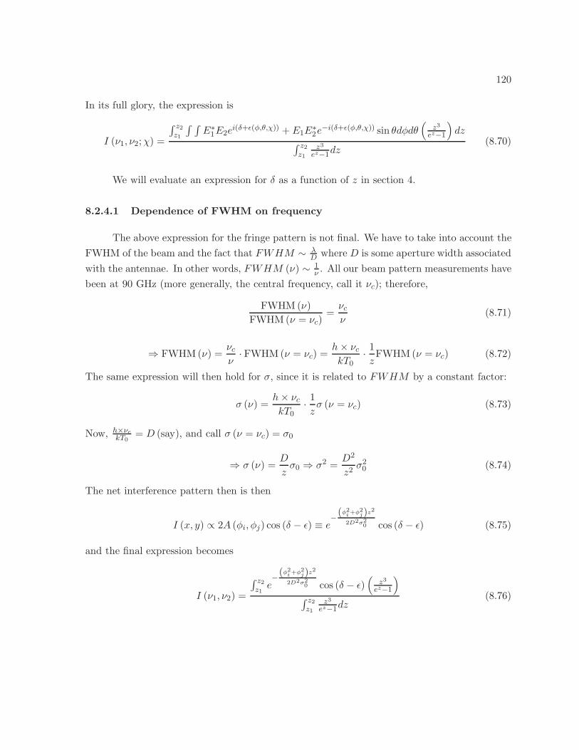
120
In its full glory, the expression is
I (ν1, ν2;χ) =
∫ z2z1
∫ ∫E∗
1E2ei(δ+ǫ(φ,θ,χ)) + E1E
∗2e
−i(δ+ǫ(φ,θ,χ)) sin θdφdθ(
z3
ez−1
)
dz∫ z2z1
z3
ez−1dz(8.70)
We will evaluate an expression for δ as a function of z in section 4.
8.2.4.1 Dependence of FWHM on frequency
The above expression for the fringe pattern is not final. We have to take into account the
FWHM of the beam and the fact that FWHM ∼ λD where D is some aperture width associated
with the antennae. In other words, FWHM (ν) ∼ 1ν . All our beam pattern measurements have
been at 90 GHz (more generally, the central frequency, call it νc); therefore,
FWHM (ν)
FWHM (ν = νc)=νcν
(8.71)
⇒ FWHM (ν) =νcν· FWHM (ν = νc) =
h× νckT0
· 1zFWHM (ν = νc) (8.72)
The same expression will then hold for σ, since it is related to FWHM by a constant factor:
σ (ν) =h× νckT0
· 1zσ (ν = νc) (8.73)
Now, h×νc
kT0= D (say), and call σ (ν = νc) = σ0
⇒ σ (ν) =D
zσ0 ⇒ σ2 =
D2
z2σ2
0 (8.74)
The net interference pattern then is then
I (x, y) ∝ 2A (φi, φj) cos (δ − ǫ) ≡ e−(φ2
i +φ2j)z2
2D2σ20 cos (δ − ǫ) (8.75)
and the final expression becomes
I (ν1, ν2) =
∫ z2z1e−(φ2
i +φ2j)z2
2D2σ20 cos (δ − ǫ)
(z3
ez−1
)
∫ z2z1
z3
ez−1dz(8.76)
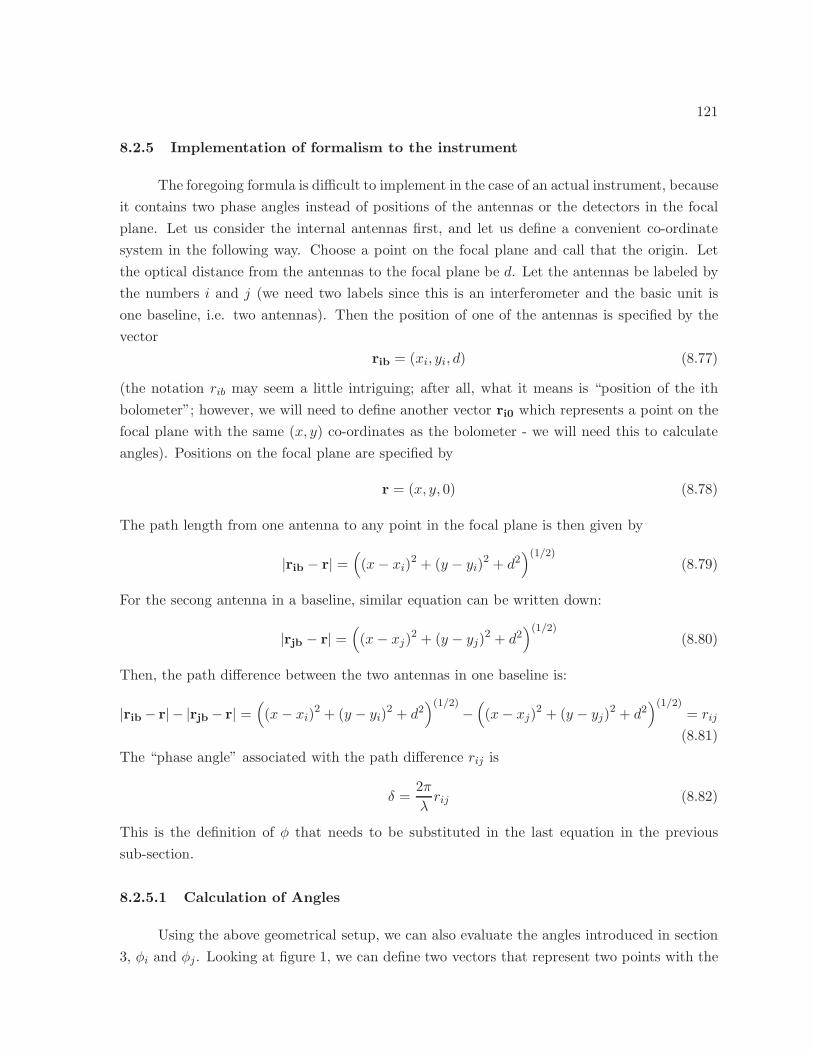
121
8.2.5 Implementation of formalism to the instrument
The foregoing formula is difficult to implement in the case of an actual instrument, because
it contains two phase angles instead of positions of the antennas or the detectors in the focal
plane. Let us consider the internal antennas first, and let us define a convenient co-ordinate
system in the following way. Choose a point on the focal plane and call that the origin. Let
the optical distance from the antennas to the focal plane be d. Let the antennas be labeled by
the numbers i and j (we need two labels since this is an interferometer and the basic unit is
one baseline, i.e. two antennas). Then the position of one of the antennas is specified by the
vector
rib = (xi, yi, d) (8.77)
(the notation rib may seem a little intriguing; after all, what it means is “position of the ith
bolometer”; however, we will need to define another vector ri0 which represents a point on the
focal plane with the same (x, y) co-ordinates as the bolometer - we will need this to calculate
angles). Positions on the focal plane are specified by
r = (x, y, 0) (8.78)
The path length from one antenna to any point in the focal plane is then given by
|rib − r| =(
(x− xi)2 + (y − yi)2 + d2)(1/2)
(8.79)
For the secong antenna in a baseline, similar equation can be written down:
|rjb − r| =(
(x− xj)2 + (y − yj)2 + d2)(1/2)
(8.80)
Then, the path difference between the two antennas in one baseline is:
|rib− r| − |rjb− r| =(
(x− xi)2 + (y − yi)2 + d2)(1/2)
−(
(x− xj)2 + (y − yj)2 + d2)(1/2)
= rij
(8.81)
The “phase angle” associated with the path difference rij is
δ =2π
λrij (8.82)
This is the definition of φ that needs to be substituted in the last equation in the previous
sub-section.
8.2.5.1 Calculation of Angles
Using the above geometrical setup, we can also evaluate the angles introduced in section
3, φi and φj. Looking at figure 1, we can define two vectors that represent two points with the
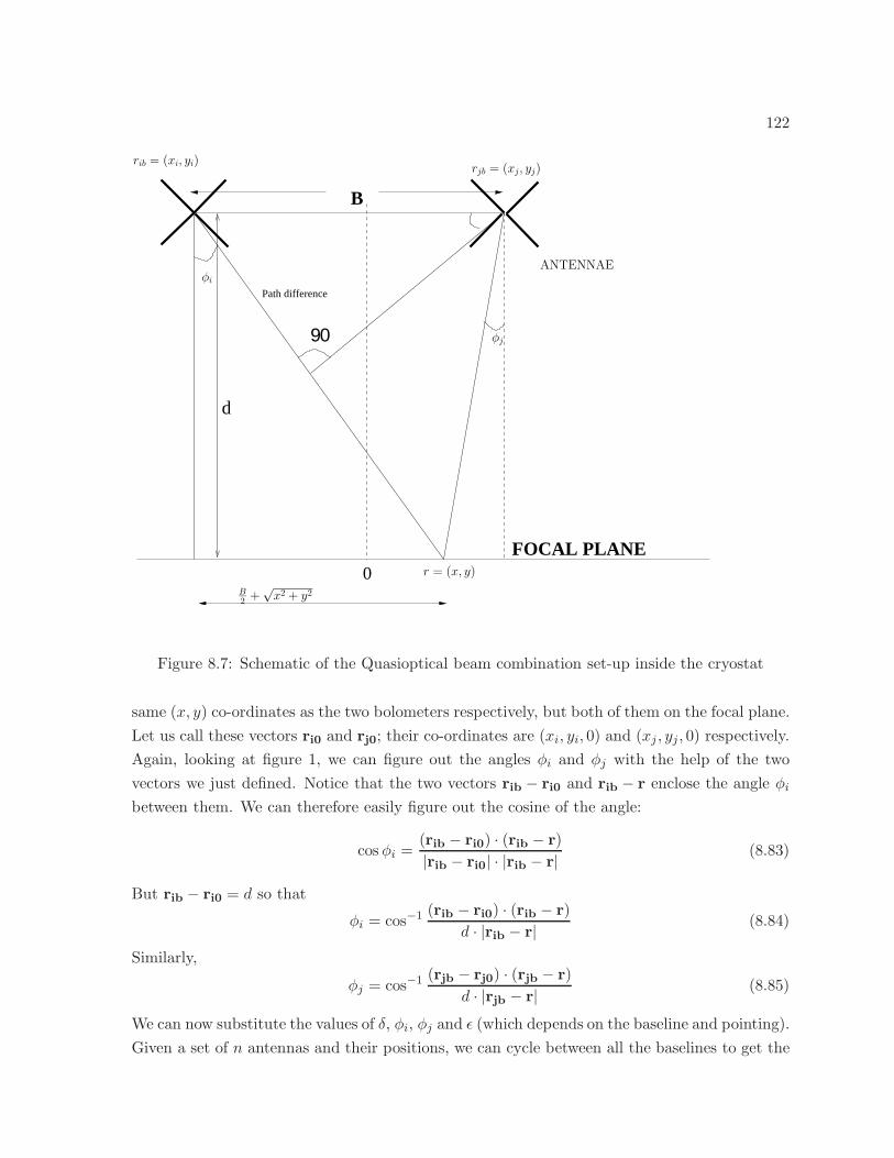
122
d
90
B
0
Path difference
FOCAL PLANE
φj
r = (x, y)
φi
B2 +√
x2 + y2
rib = (xi, yi)rjb = (xj, yj)
ANTENNAE
Figure 8.7: Schematic of the Quasioptical beam combination set-up inside the cryostat
same (x, y) co-ordinates as the two bolometers respectively, but both of them on the focal plane.
Let us call these vectors ri0 and rj0; their co-ordinates are (xi, yi, 0) and (xj , yj, 0) respectively.
Again, looking at figure 1, we can figure out the angles φi and φj with the help of the two
vectors we just defined. Notice that the two vectors rib − ri0 and rib − r enclose the angle φi
between them. We can therefore easily figure out the cosine of the angle:
cosφi =(rib − ri0) · (rib − r)
|rib − ri0| · |rib − r| (8.83)
But rib − ri0 = d so that
φi = cos−1 (rib − ri0) · (rib − r)
d · |rib − r| (8.84)
Similarly,
φj = cos−1 (rjb − rj0) · (rjb − r)
d · |rjb − r| (8.85)
We can now substitute the values of δ, φi, φj and ǫ (which depends on the baseline and pointing).
Given a set of n antennas and their positions, we can cycle between all the baselines to get the
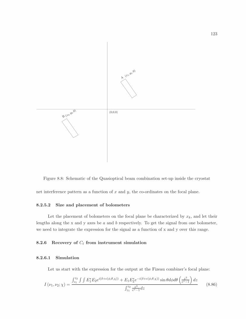
123
B
(0,0,0)
(x2,y2,
0)
A(x1,
y1,0)
Figure 8.8: Schematic of the Quasioptical beam combination set-up inside the cryostat
net interference pattern as a function of x and y, the co-ordinates on the focal plane.
8.2.5.2 Size and placement of bolometers
Let the placement of bolometers on the focal plane be characterized by xk, and let their
lengths along the x and y axes be a and b respectively. To get the signal from one bolometer,
we need to integrate the expression for the signal as a function of x and y over this range.
8.2.6 Recovery of Cℓ from instrument simulation
8.2.6.1 Simulation
Let us start with the expression for the output at the Fizeau combiner’s focal plane:
I (ν1, ν2;χ) =
∫ z2z1
∫ ∫E∗
1E2ei(δ+ǫ(φ,θ,χ)) + E1E
∗2e
−i(δ+ǫ(φ,θ,χ)) sin θdφdθ(
z3
ez−1
)
dz∫ z2z1
z3
ez−1dz(8.86)
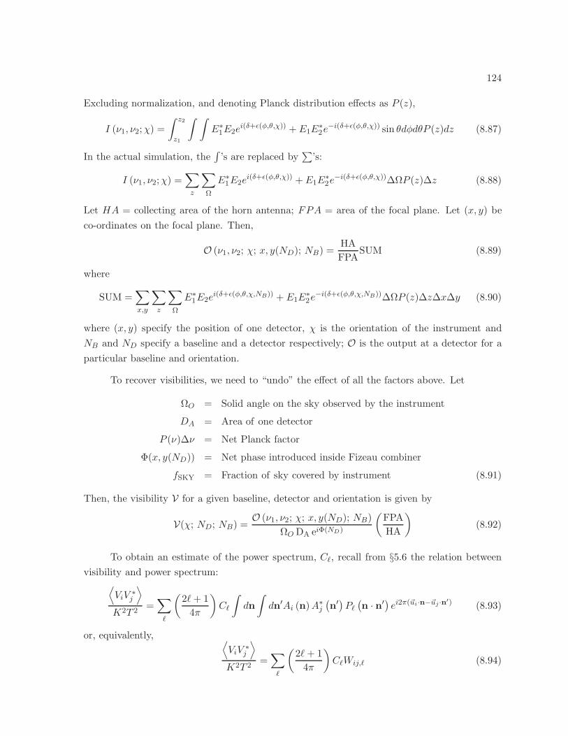
124
Excluding normalization, and denoting Planck distribution effects as P (z),
I (ν1, ν2;χ) =
∫ z2
z1
∫ ∫
E∗1E2e
i(δ+ǫ(φ,θ,χ)) + E1E∗2e
−i(δ+ǫ(φ,θ,χ)) sin θdφdθP (z)dz (8.87)
In the actual simulation, the∫
’s are replaced by∑
’s:
I (ν1, ν2;χ) =∑
z
∑
Ω
E∗1E2e
i(δ+ǫ(φ,θ,χ)) + E1E∗2e
−i(δ+ǫ(φ,θ,χ))∆ΩP (z)∆z (8.88)
Let HA = collecting area of the horn antenna; FPA = area of the focal plane. Let (x, y) be
co-ordinates on the focal plane. Then,
O (ν1, ν2; χ; x, y(ND); NB) =HA
FPASUM (8.89)
where
SUM =∑
x,y
∑
z
∑
Ω
E∗1E2e
i(δ+ǫ(φ,θ,χ,NB)) + E1E∗2e
−i(δ+ǫ(φ,θ,χ,NB))∆ΩP (z)∆z∆x∆y (8.90)
where (x, y) specify the position of one detector, χ is the orientation of the instrument and
NB and ND specify a baseline and a detector respectively; O is the output at a detector for a
particular baseline and orientation.
To recover visibilities, we need to “undo” the effect of all the factors above. Let
ΩO = Solid angle on the sky observed by the instrument
DA = Area of one detector
P (ν)∆ν = Net Planck factor
Φ(x, y(ND)) = Net phase introduced inside Fizeau combiner
fSKY = Fraction of sky covered by instrument (8.91)
Then, the visibility V for a given baseline, detector and orientation is given by
V(χ; ND; NB) =O (ν1, ν2; χ; x, y(ND); NB)
ΩO DA eiΦ(ND)
(FPA
HA
)
(8.92)
To obtain an estimate of the power spectrum, Cℓ, recall from §5.6 the relation between
visibility and power spectrum:⟨
ViV∗j
⟩
K2T 2=∑
ℓ
(2ℓ+ 1
4π
)
Cℓ
∫
dn
∫
dn′Ai (n)A∗j
(n′)Pℓ
(n · n′) ei2π(~ui·n−~uj ·n′) (8.93)
or, equivalently, ⟨
ViV∗j
⟩
K2T 2=∑
ℓ
(2ℓ+ 1
4π
)
CℓWij,ℓ (8.94)
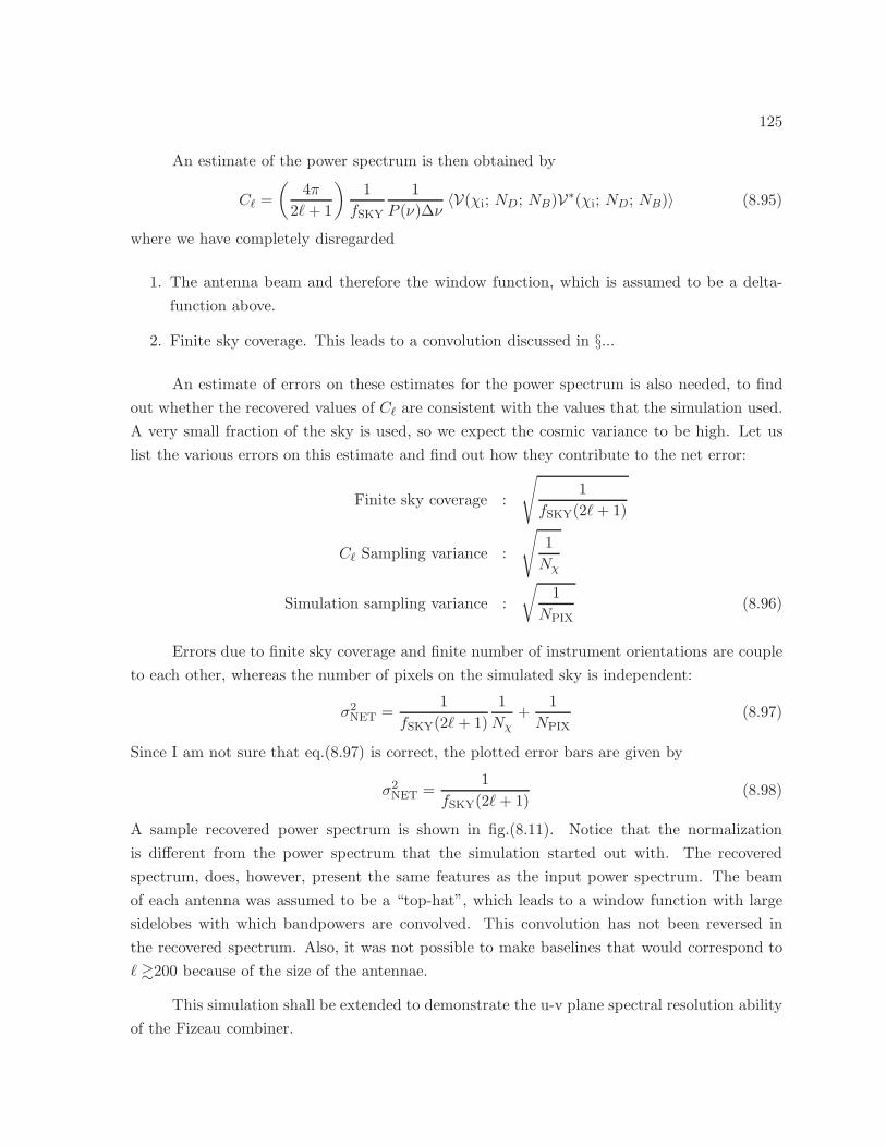
125
An estimate of the power spectrum is then obtained by
Cℓ =
(4π
2ℓ+ 1
)1
fSKY
1
P (ν)∆ν〈V(χi; ND; NB)V∗(χi; ND; NB)〉 (8.95)
where we have completely disregarded
1. The antenna beam and therefore the window function, which is assumed to be a delta-
function above.
2. Finite sky coverage. This leads to a convolution discussed in §...
An estimate of errors on these estimates for the power spectrum is also needed, to find
out whether the recovered values of Cℓ are consistent with the values that the simulation used.
A very small fraction of the sky is used, so we expect the cosmic variance to be high. Let us
list the various errors on this estimate and find out how they contribute to the net error:
Finite sky coverage :
√
1
fSKY(2ℓ+ 1)
Cℓ Sampling variance :
√
1
Nχ
Simulation sampling variance :
√1
NPIX(8.96)
Errors due to finite sky coverage and finite number of instrument orientations are couple
to each other, whereas the number of pixels on the simulated sky is independent:
σ2NET =
1
fSKY(2ℓ+ 1)
1
Nχ+
1
NPIX(8.97)
Since I am not sure that eq.(8.97) is correct, the plotted error bars are given by
σ2NET =
1
fSKY(2ℓ+ 1)(8.98)
A sample recovered power spectrum is shown in fig.(8.11). Notice that the normalization
is different from the power spectrum that the simulation started out with. The recovered
spectrum, does, however, present the same features as the input power spectrum. The beam
of each antenna was assumed to be a “top-hat”, which leads to a window function with large
sidelobes with which bandpowers are convolved. This convolution has not been reversed in
the recovered spectrum. Also, it was not possible to make baselines that would correspond to
ℓ &200 because of the size of the antennae.
This simulation shall be extended to demonstrate the u-v plane spectral resolution ability
of the Fizeau combiner.
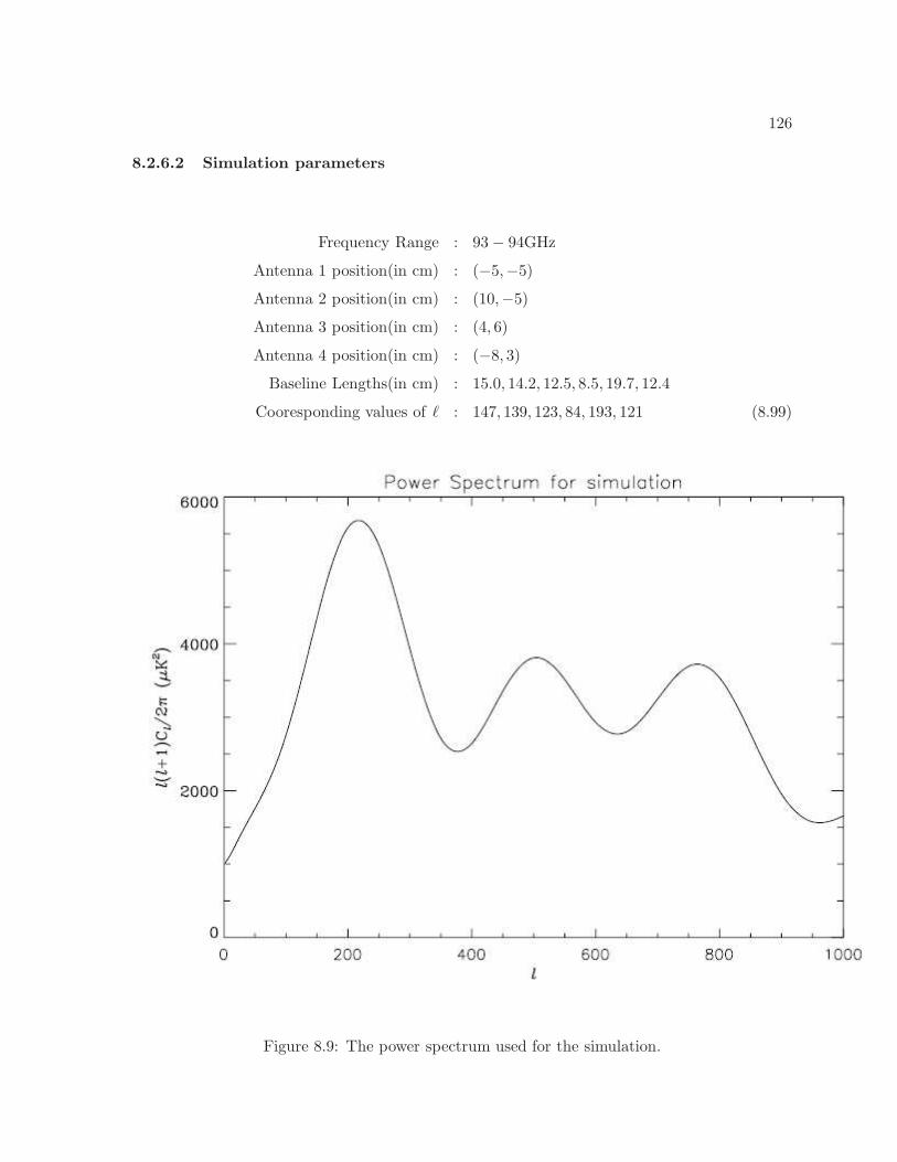
126
8.2.6.2 Simulation parameters
Frequency Range : 93− 94GHz
Antenna 1 position(in cm) : (−5,−5)
Antenna 2 position(in cm) : (10,−5)
Antenna 3 position(in cm) : (4, 6)
Antenna 4 position(in cm) : (−8, 3)
Baseline Lengths(in cm) : 15.0, 14.2, 12.5, 8.5, 19.7, 12.4
Cooresponding values of ℓ : 147, 139, 123, 84, 193, 121 (8.99)
Figure 8.9: The power spectrum used for the simulation.
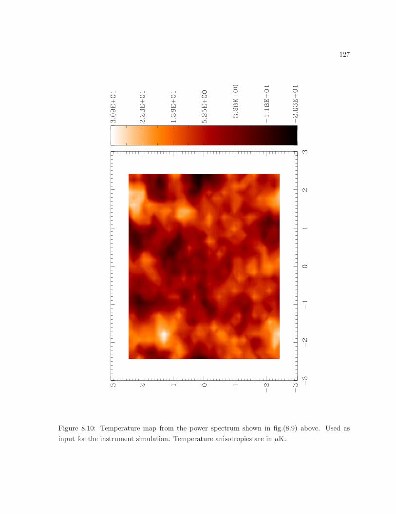
127
Figure 8.10: Temperature map from the power spectrum shown in fig.(8.9) above. Used as
input for the instrument simulation. Temperature anisotropies are in µK.
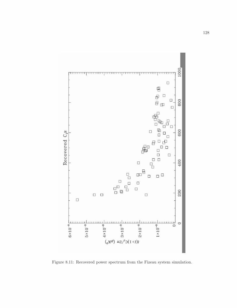
128
Figure 8.11: Recovered power spectrum from the Fizeau system simulation.
129
Bibliography
[1] M. Zaldarriaga and U. Seljak, “CMBFAST for Spatially Closed Universes,” ApJ Suppl.,
vol. 129, pp. 431–434, Aug. 2000.
[2] M. White, J. E. Carlstrom, M. Dragovan, and W. L. Holzapfel, “Interferometric Observation
of Cosmic Microwave Background Anisotropies,” ApJ, vol. 514, pp. 12–24, Mar. 1999.
130
Chapter 9
CMB Data Analysis
For almost three decades after Penzias and Wilson’s discovery, the task of finding anisotropies
in the CMB remained a challenge. COBE brought about a revolution when it reported a
detection on a 7 angular scale. A number of smaller instruments focused on smaller angular
scales followed, and in a short period of time, the size of the datasets exceeded capabilities of
the techniques used to analyze the data. Developement of analysis techniques has been the
prime focus of theorists in CMB ever since. In addition, experiments like DASI have upped the
stakes because they use interferometry. In a way, interferometry has some advantages, since it
enables sampling directly from fourier space, i.e. directly from the l-modes themselves, which is
precisely what we aim for in power spectrum estimation. However, interferometers come with
their own challenges.
In this chapter, we start with a concise discussion of linear mapmaking techniques in §9.1.We then move to Bayesian Maximum-likelihood Analysis of interferometry data to recover Cℓ’s
and show that a full Bayesian approach is computationally unfeasible. In section 4, we explore
a novel approach to likelihood analysis that enables computationally efficient calculation within
a fully Bayesian framework, without having to make approximations. This is the first time this
technique (called “Gibbs sampling”) has been applied to interferometry. We then present results
and show that Gibbs sampling as used here is indeed robust by applying the Gelman-Rubins
test for convergence.
9.1 Mapmaking
9.1.1 The general mapmaking problem
This section is a concise summary of the detailed discussion in [1].
In general, every instrument has its own unique scan strategy, and what we receive (in our
131
case, the visibility from some baseline) depends on the signal on the sky, and the convolution
with the beam, combined with the scan strategy. Instrumental noise has to be added to that
later. All this is summarized in the nice equation
d = P∆ + n (9.1)
where d is TOD (“time-ordered data”), ∆ is the signal we are trying to recover, n is instrumental
noise, and P has all the information about our scan strategy. Bear in mind in the discussion
that follows that d, ∆ and n are vectors, i.e. column matrices (one could take them to be row
matrices just as well, since the final results will be exactly the same), and P is a matrix with
the correct dimensions.
In order to make a map, then (or, for that matter, do any analysis), we need to recover
∆, the signal on the sy; in our case, the visibility from different baselines. We therefore need
to invert the above equation to recover ∆. While it isn’t clear to me whether there is a finite
number of non-linear methods, our first task should be to find linear solutions. All linear
solutions can be expressed as
∆′ = Bd (9.2)
W.L.O.G., where ∆′ is an estimate of ∆, and therefore, there is an estimation error involved,
no matter how good our technique. Before we jump into calculating B, let us define a few basic
quantities. Let S =⟨∆∆T
⟩denote the theory covariance matrix, and N =
⟨nnT
⟩the noise
covariance matrix. It seems reasonable to me (do let me know if you object, and why, since
I may have missed something) to suppose that noise and signal are uncorrelated, since their
sources have nothing to do with each other, i.e.⟨∆nT
⟩=⟨n∆T
⟩≡ 0
We are now ready to address the mapmaking problem. What follows is a discussion of
my own analysis, and unfortunately, I haven’t been able to compare it to any reference to see
whether it has any element of sensibility. What I found is that broadly, there are three different
conditions on can impose, and each will lead to a different (and unique) definition of B. The
three conditions are:
1. Ease of calculation
2. Minimizing the estimation error
3. Minimizing χ2
Let us look at these in detail.
132
9.1.1.1 The Brute-force simplistic method
In the equation
d = P∆ + n (9.3)
the simplest thing to do to recover ∆ is to multiply throughout by P−1 to get
P−1d = ∆ + P−1n (9.4)
so that
∆′ = P−1d (9.5)
with an estimation error
δ = P−1n (9.6)
However, we CANNOT possibly do the inverse operation on P, since it is not a square matrix.
But we can do other operations, like taking the transpose. So we recall that PTP is the modulus
of P. This is a square matrix, and we can take its inverse, which is, schematically P−1(PT)−1
(I say schematically, because the operation inverse is not permitted on the individual matrices).
Clearly, if we multiply this by PT , we can recover P. The net matrix is then(PTP
)−1PT .
If we look at the last equation more carefully, we may perhaps be persuaded to feel a
little less silly for adopting such a simplistic approach, since it tells us that the estimation error
is independent of signal, and depends only on instrumental noise. While this is nice, we may
not entirely be happy with it and want to minimize |δ|2.
9.1.1.2 Minimizing the estimation error
In general, we want to estimate ∆ by a “correction matrix”; call it B:
∆′ = Bd = BP∆ + Bn (9.7)
so that the estimation error is
δ = ∆′ −∆ = BP∆ + Bn−∆ = (BP− I)∆ + Bn (9.8)
Therefore,
|δ|2 =⟨δδT⟩
=⟨[(BP− I)∆ + Bn]
[∆T
(PTBT − I
)+ nTBT
]⟩(9.9)
Multiplying out explicitly,
|δ|2 =⟨(BP− I)∆∆T
(PTBT − I
)+ BnnTBT +
[Bn∆T
(PTBT − I
)+ (BP− I)∆nTBT
]⟩
(9.10)
133
The two terms in the square brackets are ∝ either⟨∆nT
⟩or its transpose, both of which are
zero. Therefore,
|δ|2 =⟨(BP− I)∆∆T
(PTBT − I
)+ BnnTBT
⟩(9.11)
Substituting S =⟨∆∆T
⟩and N =
⟨nnT
⟩, we get
|δ|2 = (BP− I)S(PTBT − I
)+ BNBT (9.12)
Now, we need a B such that |δ|2 is minimized. Therefore, we need a solution to the equation
∂|δ|2∂B
= 0 (9.13)
Differentiating w.r.t. B, we get
PS(PTBT − I
)+ NBT = 0 (9.14)
Collecting terms with BT
(PSPT + N
)BT −PS = 0 (9.15)
or(PSPT + N
)BT = PS (9.16)
On a first glance, it seems like solving this equation is impossible for any value of BT , because
if we define BT such that it cancels out either term inside the brackets, it is impossible to make
the LHS equal to PS.
However, we can always cancel out the bracket in the LHS by defining a BT that is ∝ its
inverse. If we also require that BT is simultaneously ∝ PS, then we have essentially solved the
equation. Formally, the solution is
BT =(PSPT + N
)−1PS (9.17)
All we need to do now is to take the transpose of the RHS, and we will have our solution, i.e.
B = (PS)T((
PSPT + N)T)−1
(9.18)
where we have used the fact that (AB)T = BTAT . We can now expand out to get
B =(STPT
) ((PSPT
)T+ NT
)−1(9.19)
But for S, ST =(∆∆T
)T=(∆T)T
∆T = ∆∆T = S, and similarly, NT = N. Now(PSPT
)T= (SP)T PT =
(PT)T
STPT = PSPT . So the final expression is
B = SPT[PSPT + N
]−1(9.20)
We could have differentiated |δ|2 w.r.t. BT instead, and we would get precisely the same result.
134
9.1.1.3 Minimizing χ2
Following the discussion in [2] §11.5 (equations 11.129 to 11.131),
χ2 = (d−P∆)N−1 (d−P∆) (9.21)
To minimize χ2, we set∂χ2
∂∆= 0 (9.22)
which gives us
∆′ =(PTN−1P
)−1PTN−1d (9.23)
⇒ B =(PTN−1P
)−1PTN−1 (9.24)
This map-making method can be employed to extract a “fourier map”; in other words, visi-
bilities, from an interferometer. However, the method involves a number of matrix inversions,
each of which costs ∼ N3P operations where NP is the number of pixels in the map (in fourier or
real space). Wandelt et al ([3, 4]) have introduced fully Bayesian methods that allow a global
inference of covariance and allow map recovery at the same time, and cost only N32
P operations.
This method (called “Gibbs sampling”) will be discussed in §.. The true advantages of Gibbs
sampling come to light when power spectra need to be evaluated.
9.2 Power Spectrum Estimation: Bayesian Approach
Let d = pixelized data from an interferometer. We wish to explore the posterior density
P (Cℓ|d) ∝ P (d|Cℓ)P (Cℓ)← Prior (9.25)
where
P (d|Cℓ) ∝ exp(
d†C−1D d
)
(9.26)
where
C−1D = S (Cℓ) +N (9.27)
is the covariance matrix.
Traditionally, least-squares [5] and maximum-likelihood [6] estimators have been em-
ployed to explore the posterior. However, evaluating either is computationally very costly,
requiring O(N3P
)operations.
135
9.2.1 Detailed Bayesian Formalism
In the Bayesian approach, we wish to compute the posterior density
P (Cℓ, s|d) =P (d|s)P (s|Cℓ)P (Cℓ)
P (d)(9.28)
If S and N are signal and noise covariance matrices respectively,
P (d|s) =1
√
2π |N |exp
(
−1
2(d− s)†N−1 (d− s)
)
(9.29)
Also, since we know that the CMB is very nearly gaussian
P (s|Cℓ) =1
√
2π |S|exp
(
−1
2s†S−1s
)
(9.30)
so that
− lnP (Cℓ, s|d) =1
2(d− s)†N−1 (d− s) +
1
2s†S−1s+
1
2ln |S| (9.31)
The best estimate of the signal s can then be found by
∂ (− lnP (Cℓ, s|d))∂s†
= −N−1 (d− s) + S−1s = 0
=⇒(S−1 +N−1
)sBE = N−1d (9.32)
Matrix inversions are computationally costly, and in the final expression for sBE, there are
three inversions, each costing O(N3P
)operations. If we were to transform the above equation
into the form Ax = B, we can employ efficient techniques to solve for sBE.
However, an efficient method of extracting sBE leaves the problem of Cℓ extraction being
extremely time-consuming computationally.
9.2.2 The problem with the Bayesian approach
Interferometry has been used to detect CMB temperature and polarization anisotropy
(VSA, DASI, CBI references). Here are some of the advantages of interferometry:
1. Direct sampling of Fourier space
2. No leakage T → Q,U , so better control of systematic effects
However, an exact Bayesian analysis analysis method is just as unfeasible as for an imaging
experiment. However, Wandelt et al[3] have introduced a fully Bayesian approach - Gibbs
sampling - that allows a global inference of covariance. Among the many advantages of using
the Gibbs sampler is that it is easily extended for foreground removal.
Let us first illustrate Gibbs’ sampling by applying it to a simple problem in the next
section.
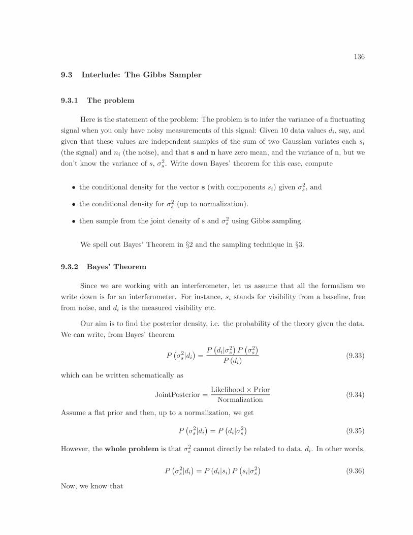
136
9.3 Interlude: The Gibbs Sampler
9.3.1 The problem
Here is the statement of the problem: The problem is to infer the variance of a fluctuating
signal when you only have noisy measurements of this signal: Given 10 data values di, say, and
given that these values are independent samples of the sum of two Gaussian variates each si
(the signal) and ni (the noise), and that s and n have zero mean, and the variance of n, but we
don’t know the variance of s, σ2s . Write down Bayes’ theorem for this case, compute
• the conditional density for the vector s (with components si) given σ2s , and
• the conditional density for σ2s (up to normalization).
• then sample from the joint density of s and σ2s using Gibbs sampling.
We spell out Bayes’ Theorem in §2 and the sampling technique in §3.
9.3.2 Bayes’ Theorem
Since we are working with an interferometer, let us assume that all the formalism we
write down is for an interferometer. For instance, si stands for visibility from a baseline, free
from noise, and di is the measured visibility etc.
Our aim is to find the posterior density, i.e. the probability of the theory given the data.
We can write, from Bayes’ theorem
P(σ2s |di)
=P(di|σ2
s
)P(σ2s
)
P (di)(9.33)
which can be written schematically as
JointPosterior =Likelihood × Prior
Normalization(9.34)
Assume a flat prior and then, up to a normalization, we get
P(σ2s |di
)= P
(di|σ2
s
)(9.35)
However, the whole problem is that σ2s cannot directly be related to data, di. In other words,
P(σ2s |di)
= P (di|si)P(si|σ2
s
)(9.36)
Now, we know that
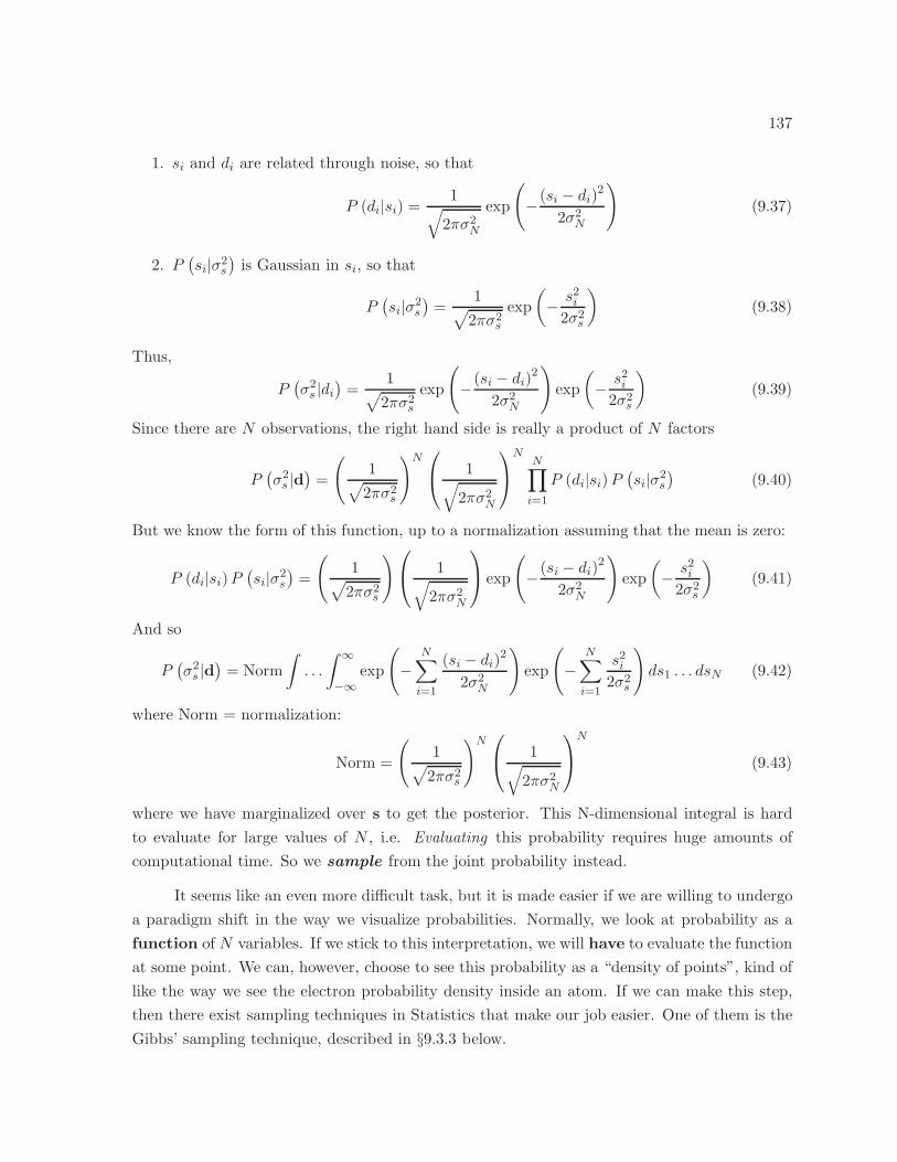
137
1. si and di are related through noise, so that
P (di|si) =1
√
2πσ2N
exp
(
−(si − di)22σ2
N
)
(9.37)
2. P(si|σ2
s
)is Gaussian in si, so that
P(si|σ2
s
)=
1√
2πσ2s
exp
(
− s2i2σ2
s
)
(9.38)
Thus,
P(σ2s |di
)=
1√
2πσ2s
exp
(
−(si − di)22σ2
N
)
exp
(
− s2i2σ2
s
)
(9.39)
Since there are N observations, the right hand side is really a product of N factors
P(σ2s |d)
=
(
1√
2πσ2s
)N
1
√
2πσ2N
NN∏
i=1
P (di|si)P(si|σ2
s
)(9.40)
But we know the form of this function, up to a normalization assuming that the mean is zero:
P (di|si)P(si|σ2
s
)=
(
1√
2πσ2s
)
1
√
2πσ2N
exp
(
−(si − di)22σ2
N
)
exp
(
− s2i2σ2
s
)
(9.41)
And so
P(σ2s |d)
= Norm
∫
. . .
∫ ∞
−∞exp
(
−N∑
i=1
(si − di)22σ2
N
)
exp
(
−N∑
i=1
s2i2σ2
s
)
ds1 . . . dsN (9.42)
where Norm = normalization:
Norm =
(
1√
2πσ2s
)N
1
√
2πσ2N
N
(9.43)
where we have marginalized over s to get the posterior. This N-dimensional integral is hard
to evaluate for large values of N , i.e. Evaluating this probability requires huge amounts of
computational time. So we sample from the joint probability instead.
It seems like an even more difficult task, but it is made easier if we are willing to undergo
a paradigm shift in the way we visualize probabilities. Normally, we look at probability as a
function of N variables. If we stick to this interpretation, we will have to evaluate the function
at some point. We can, however, choose to see this probability as a “density of points”, kind of
like the way we see the electron probability density inside an atom. If we can make this step,
then there exist sampling techniques in Statistics that make our job easier. One of them is the
Gibbs’ sampling technique, described in §9.3.3 below.
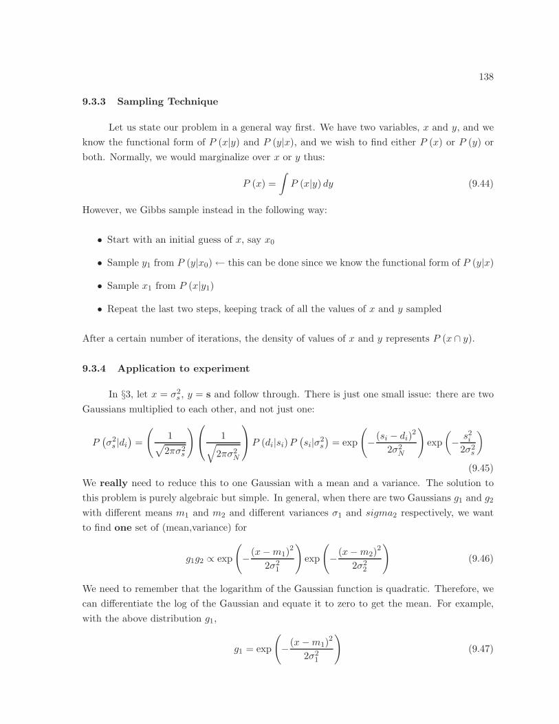
138
9.3.3 Sampling Technique
Let us state our problem in a general way first. We have two variables, x and y, and we
know the functional form of P (x|y) and P (y|x), and we wish to find either P (x) or P (y) or
both. Normally, we would marginalize over x or y thus:
P (x) =
∫
P (x|y) dy (9.44)
However, we Gibbs sample instead in the following way:
• Start with an initial guess of x, say x0
• Sample y1 from P (y|x0)← this can be done since we know the functional form of P (y|x)
• Sample x1 from P (x|y1)
• Repeat the last two steps, keeping track of all the values of x and y sampled
After a certain number of iterations, the density of values of x and y represents P (x ∩ y).
9.3.4 Application to experiment
In §3, let x = σ2s , y = s and follow through. There is just one small issue: there are two
Gaussians multiplied to each other, and not just one:
P(σ2s |di
)=
(
1√
2πσ2s
)
1
√
2πσ2N
P (di|si)P(si|σ2
s
)= exp
(
−(si − di)22σ2
N
)
exp
(
− s2i2σ2
s
)
(9.45)
We really need to reduce this to one Gaussian with a mean and a variance. The solution to
this problem is purely algebraic but simple. In general, when there are two Gaussians g1 and g2
with different means m1 and m2 and different variances σ1 and sigma2 respectively, we want
to find one set of (mean,variance) for
g1g2 ∝ exp
(
−(x−m1)2
2σ21
)
exp
(
−(x−m2)2
2σ22
)
(9.46)
We need to remember that the logarithm of the Gaussian function is quadratic. Therefore, we
can differentiate the log of the Gaussian and equate it to zero to get the mean. For example,
with the above distribution g1,
g1 = exp
(
−(x−m1)2
2σ21
)
(9.47)
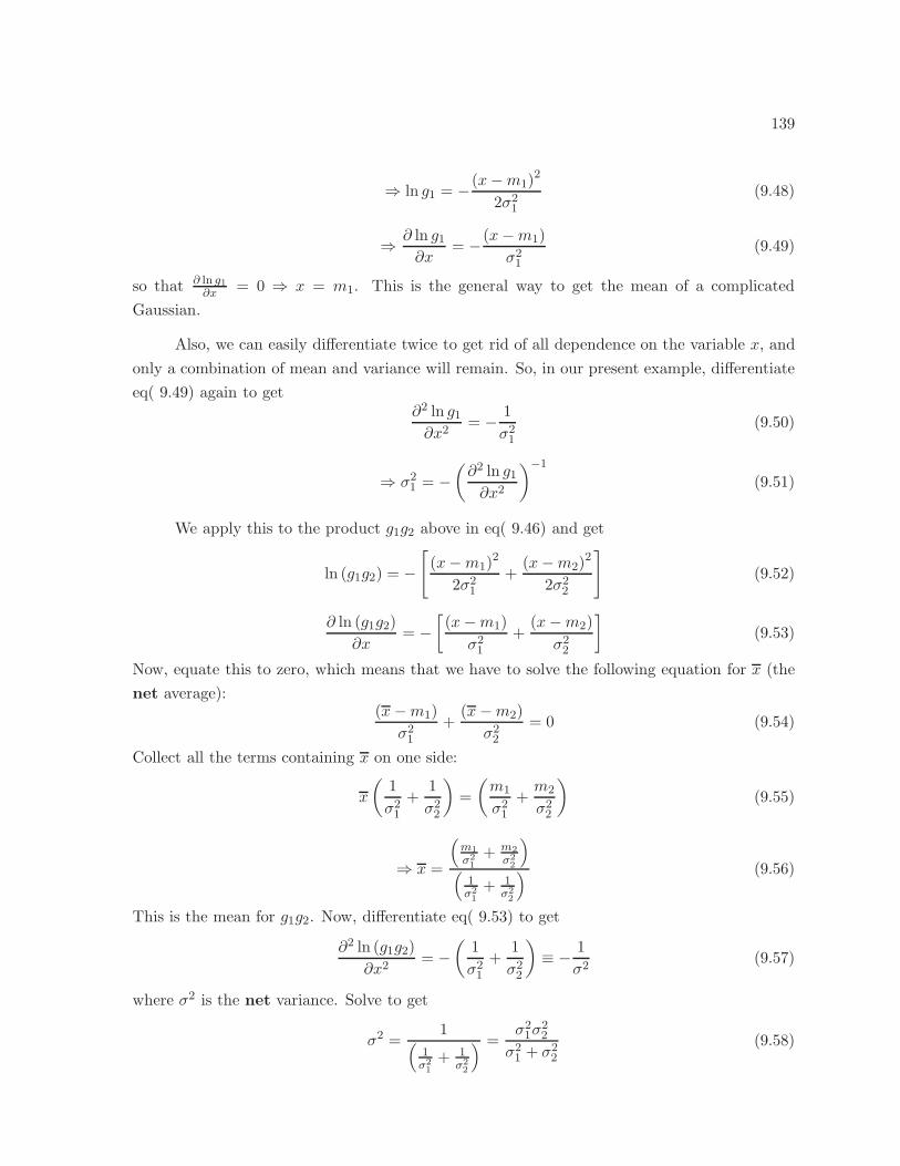
139
⇒ ln g1 = −(x−m1)2
2σ21
(9.48)
⇒ ∂ ln g1∂x
= −(x−m1)
σ21
(9.49)
so that ∂ ln g1∂x = 0 ⇒ x = m1. This is the general way to get the mean of a complicated
Gaussian.
Also, we can easily differentiate twice to get rid of all dependence on the variable x, and
only a combination of mean and variance will remain. So, in our present example, differentiate
eq( 9.49) again to get∂2 ln g1∂x2
= − 1
σ21
(9.50)
⇒ σ21 = −
(∂2 ln g1∂x2
)−1
(9.51)
We apply this to the product g1g2 above in eq( 9.46) and get
ln (g1g2) = −[
(x−m1)2
2σ21
+(x−m2)
2
2σ22
]
(9.52)
∂ ln (g1g2)
∂x= −
[(x−m1)
σ21
+(x−m2)
σ22
]
(9.53)
Now, equate this to zero, which means that we have to solve the following equation for x (the
net average):(x−m1)
σ21
+(x−m2)
σ22
= 0 (9.54)
Collect all the terms containing x on one side:
x
(1
σ21
+1
σ22
)
=
(m1
σ21
+m2
σ22
)
(9.55)
⇒ x =
(m1
σ21
+ m2
σ22
)
(1σ21
+ 1σ22
) (9.56)
This is the mean for g1g2. Now, differentiate eq( 9.53) to get
∂2 ln (g1g2)
∂x2= −
(1
σ21
+1
σ22
)
≡ − 1
σ2(9.57)
where σ2 is the net variance. Solve to get
σ2 =1
(1σ21
+ 1σ22
) =σ2
1σ22
σ21 + σ2
2
(9.58)
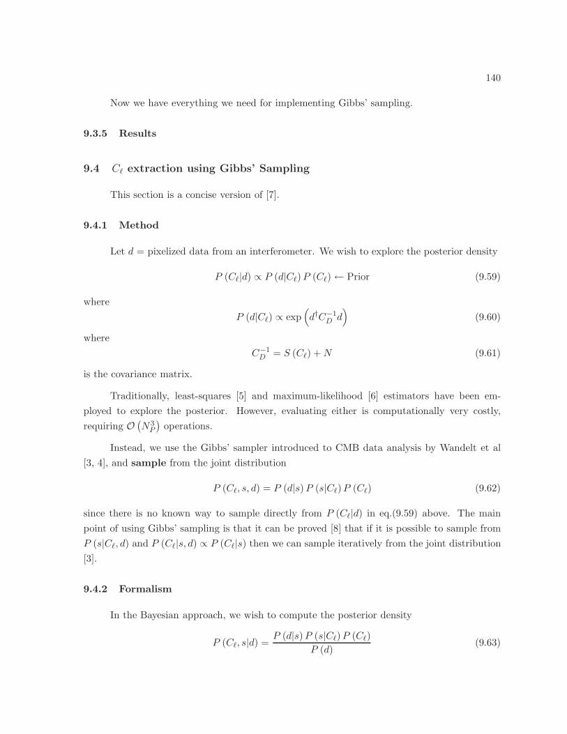
140
Now we have everything we need for implementing Gibbs’ sampling.
9.3.5 Results
9.4 Cℓ extraction using Gibbs’ Sampling
This section is a concise version of [7].
9.4.1 Method
Let d = pixelized data from an interferometer. We wish to explore the posterior density
P (Cℓ|d) ∝ P (d|Cℓ)P (Cℓ)← Prior (9.59)
where
P (d|Cℓ) ∝ exp(
d†C−1D d
)
(9.60)
where
C−1D = S (Cℓ) +N (9.61)
is the covariance matrix.
Traditionally, least-squares [5] and maximum-likelihood [6] estimators have been em-
ployed to explore the posterior. However, evaluating either is computationally very costly,
requiring O(N3P
)operations.
Instead, we use the Gibbs’ sampler introduced to CMB data analysis by Wandelt et al
[3, 4], and sample from the joint distribution
P (Cℓ, s, d) = P (d|s)P (s|Cℓ)P (Cℓ) (9.62)
since there is no known way to sample directly from P (Cℓ|d) in eq.(9.59) above. The main
point of using Gibbs’ sampling is that it can be proved [8] that if it is possible to sample from
P (s|Cℓ, d) and P (Cℓ|s, d) ∝ P (Cℓ|s) then we can sample iteratively from the joint distribution
[3].
9.4.2 Formalism
In the Bayesian approach, we wish to compute the posterior density
P (Cℓ, s|d) =P (d|s)P (s|Cℓ)P (Cℓ)
P (d)(9.63)
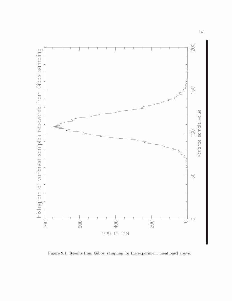
141
Figure 9.1: Results from Gibbs’ sampling for the experiment mentioned above.
142
If S and N are signal and noise covariance matrices respectively,
P (d|s) = exp
(
−1
2(d− s)†N−1 (d− s)
)
(9.64)
Also, since we know that the CMB is very nearly gaussian [ref]
P (s|Cℓ) =1
√
|S|exp
(
−1
2s†S−1s
)
(9.65)
so that
− lnP (Cℓ, s|d) =1
2(d− s)†N−1 (d− s) +
1
2s†S−1s+
1
2ln |S| (9.66)
The best estimate of the signal s can then be found by
∂ (− lnP (Cℓ, s|d))∂s†
= −N−1 (d− s) + S−1s = 0
=⇒(S−1 +N−1
)sBE = N−1d (9.67)
Matrix inversions are computationally costly, and in the final expression for sBE, there are
three inversions, each costing O(N3P
)operations. If we were to transform the above equation
into the form Ax = B, we can employ efficient techniques to solve for sBE.
We also need to remember that eq.(9.67) gives us a value for the average of the signal.
The real signal on the sky is of the form x + C12 ξ where ξ is the variation and is a gaussian
variable and C is the covariance. C is evaluated easily by noting that P is a multiple of two
gaussians, with covariances S and N ; therefore the covariance of P is
C−1 = S−1 +N−1 =⇒ C =(S−1 +N−1
)−1(9.68)
Eq.(9.67) can be recast in a more suitable format thus
(S−1 +N−1
)sBE = N−1d
=⇒ S− 12
(
1 + S12N−1S
12
)
S− 12x = N−1d
=⇒(
1 + S12N−1S
12
)
S− 12x = S
12N−1d (9.69)
where we have replaced sBE by x. We now need to find a similar equation for the fluctuating
part of the signal. Call this part b such that s = x + b. b then needs to satisfy the following
properties
〈b〉 = 0 (9.70)⟨
bb†⟩
= C, since (9.71)
b = C12 ξ (9.72)
=⇒ C−1b = C− 12 ξ (9.73)
143
We claim then that if(S−1 +N−1
)b = S− 1
2 ξ1 +N− 12 ξ2 (9.74)
then b has the properties outlined in eq.(9.73). To prove the first property, take the average of
the LHS in eq.(9.74):
(S−1 +N−1
)〈b〉 = S− 1
2 〈ξ1〉+N− 12 〈ξ2〉 ≡ 0 (9.75)
The second property is proved thus
⟨
bb†⟩
= C⟨(
S− 12 ξ1 +N− 1
2 ξ2
)(
S− 12 ξ†1 +N− 1
2 ξ†2
)⟩
C
= C(
S−1⟨
ξ1ξ†1
⟩
+N−1⟨
ξ2ξ†2
⟩)
C
= C (9.76)
where we have used the fact that ξ1 and ξ2 are independent gaussian variates with unit variance:
⟨
ξ1ξ†2
⟩
=⟨
ξ†1ξ2⟩
= 0 (9.77)⟨
ξ1ξ†1
⟩
=⟨
ξ2ξ†2
⟩
= 1 (9.78)
The equation for b is then
(S−1 +N−1
)b = S− 1
2 ξ1 +N− 12 ξ2
=⇒ S− 12
(
1 + S12N−1S
12
)
S− 12 b = S− 1
2 ξ1 +N− 12 ξ2
=⇒(
1 + S12N−1S
12
)
S− 12 b = ξ1 + S
12N− 1
2 ξ2 (9.79)
To summarize, the two equations for simulating the signal are
(
1 + S12N−1S
12
)
S− 12x = S
12N−1d (9.80)
(
1 + S12N−1S
12
)
S− 12 b = ξ1 + S
12N− 1
2 ξ2 (9.81)
These can be solved to obtain x and b for every iteration, and s = x+ b.
9.4.2.1 Beam / Window Function
Brute-force Implementation The foregoing discussion ignores the beam of the instru-
ment, which is assumed to be flat in fourier space. This assumption is unreal and the beam
needs to be included in signal and power spectrum estimation. Let us denote the signal co-
variance matrix with the “flat” beam mentioned above as SD. SD is clearly diagonal, and its
elements are the different Cℓ’s. If S is the signal covariance matrix, then, schematically,
S = BSD (9.82)
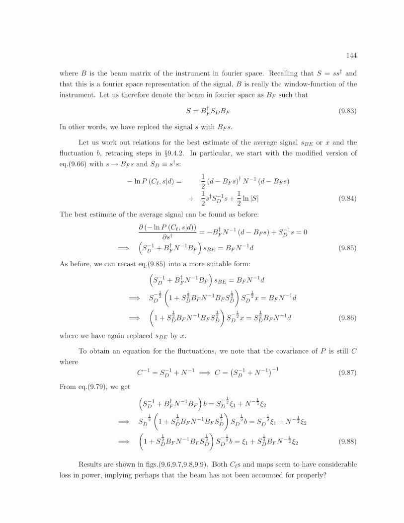
144
where B is the beam matrix of the instrument in fourier space. Recalling that S = ss† and
that this is a fourier space representation of the signal, B is really the window-function of the
instrument. Let us therefore denote the beam in fourier space as BF such that
S = B†FSDBF (9.83)
In other words, we have replced the signal s with BF s.
Let us work out relations for the best estimate of the average signal sBE or x and the
fluctuation b, retracing steps in §9.4.2. In particular, we start with the modified version of
eq.(9.66) with s→ BF s and SD ≡ s†s:
− lnP (Cℓ, s|d) =1
2(d−BF s)†N−1 (d−BF s)
+1
2s†S−1
D s+1
2ln |S| (9.84)
The best estimate of the average signal can be found as before:
∂ (− lnP (Cℓ, s|d))∂s†
= −B†FN
−1 (d−BF s) + S−1D s = 0
=⇒(
S−1D +B†
FN−1BF
)
sBE = BFN−1d (9.85)
As before, we can recast eq.(9.85) into a more suitable form:(
S−1D +B†
FN−1BF
)
sBE = BFN−1d
=⇒ S− 1
2
D
(
1 + S12
DBFN−1BFS
12
D
)
S− 1
2
D x = BFN−1d
=⇒(
1 + S12
DBFN−1BFS
12
D
)
S− 1
2
D x = S12
DBFN−1d (9.86)
where we have again replaced sBE by x.
To obtain an equation for the fluctuations, we note that the covariance of P is still C
where
C−1 = S−1D +N−1 =⇒ C =
(S−1D +N−1
)−1(9.87)
From eq.(9.79), we get
(
S−1D +B†
FN−1BF
)
b = S− 1
2
D ξ1 +N− 12 ξ2
=⇒ S− 1
2
D
(
1 + S12
DBFN−1BFS
12
D
)
S− 1
2
D b = S− 1
2
D ξ1 +N− 12 ξ2
=⇒(
1 + S12
DBFN−1BFS
12
D
)
S− 1
2
D b = ξ1 + S12
DBFN− 1
2 ξ2 (9.88)
Results are shown in figs.(9.6,9.7,9.8,9.9). Both Cℓs and maps seem to have considerable
loss in power, implying perhaps that the beam has not been accounted for properly?
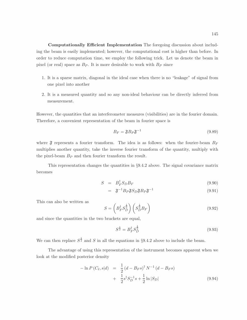
145
Computationally Efficient Implementation The foregoing discussion about includ-
ing the beam is easily implemented; however, the computational cost is higher than before. In
order to reduce computation time, we employ the following trick. Let us denote the beam in
pixel (or real) space as BP . It is more desirable to work with BP since
1. It is a sparse matrix, diagonal in the ideal case when there is no “leakage” of signal from
one pixel into another
2. It is a measured quantity and so any non-ideal behaviour can be directly inferred from
measurement.
However, the quantities that an interferometer measures (visibilities) are in the fourier domain.
Therefore, a convenient representation of the beam in fourier space is
BF = FBPF−1 (9.89)
where F represents a fourier transform. The idea is as follows: when the fourier-beam BF
multiplies another quantity, take the inverse fourier transform of the quantity, multiply with
the pixel-beam BP and then fourier transform the result.
This representation changes the quantities in §9.4.2 above. The signal covariance matrix
becomes
S = B†FSDBF (9.90)
= F−1BPFSDFBPF−1 (9.91)
This can also be written as
S =
(
B†FS
12
D
)(
S12
DBF
)
(9.92)
and since the quantities in the two brackets are equal,
S12 = B†
FS12
D (9.93)
We can then replace S12 and S in all the equations in §9.4.2 above to include the beam.
The advantage of using this representation of the instrument becomes apparent when we
look at the modified posterior density
− lnP (Cℓ, s|d) =1
2(d−BF s)†N−1 (d−BF s)
+1
2s†S−1
D s+1
2ln |SD| (9.94)
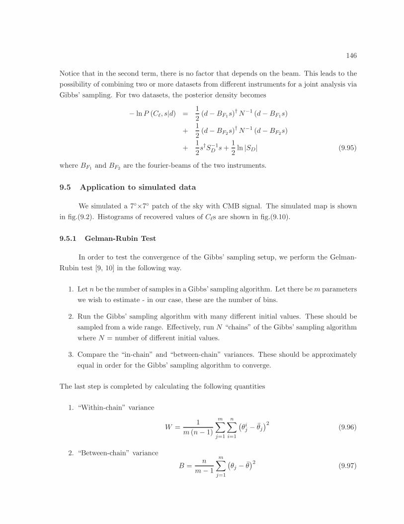
146
Notice that in the second term, there is no factor that depends on the beam. This leads to the
possibility of combining two or more datasets from different instruments for a joint analysis via
Gibbs’ sampling. For two datasets, the posterior density becomes
− lnP (Cℓ, s|d) =1
2(d−BF1
s)†N−1 (d−BF1s)
+1
2(d−BF2
s)†N−1 (d−BF2s)
+1
2s†S−1
D s+1
2ln |SD| (9.95)
where BF1and BF2
are the fourier-beams of the two instruments.
9.5 Application to simulated data
We simulated a 7×7 patch of the sky with CMB signal. The simulated map is shown
in fig.(9.2). Histograms of recovered values of Cℓs are shown in fig.(9.10).
9.5.1 Gelman-Rubin Test
In order to test the convergence of the Gibbs’ sampling setup, we perform the Gelman-
Rubin test [9, 10] in the following way.
1. Let n be the number of samples in a Gibbs’ sampling algorithm. Let there bem parameters
we wish to estimate - in our case, these are the number of bins.
2. Run the Gibbs’ sampling algorithm with many different initial values. These should be
sampled from a wide range. Effectively, run N “chains” of the Gibbs’ sampling algorithm
where N = number of different initial values.
3. Compare the “in-chain” and “between-chain” variances. These should be approximately
equal in order for the Gibbs’ sampling algorithm to converge.
The last step is completed by calculating the following quantities
1. “Within-chain” variance
W =1
m (n− 1)
m∑
j=1
n∑
i=1
(θij − θj
)2(9.96)
2. “Between-chain” variance
B =n
m− 1
m∑
j=1
(θj − θ
)2(9.97)
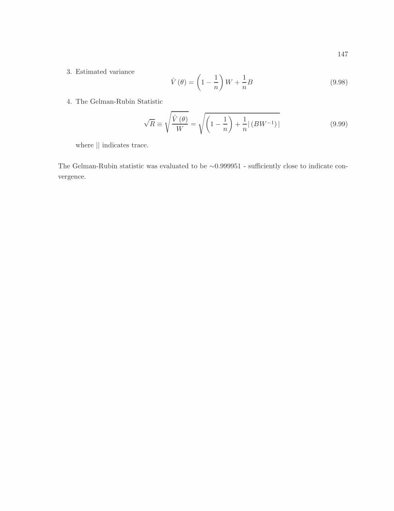
147
3. Estimated variance
V (θ) =
(
1− 1
n
)
W +1
nB (9.98)
4. The Gelman-Rubin Statistic
√R ≡
√
V (θ)
W=
√(
1− 1
n
)
+1
n| (BW−1) | (9.99)
where || indicates trace.
The Gelman-Rubin statistic was evaluated to be ∼0.999951 - sufficiently close to indicate con-
vergence.
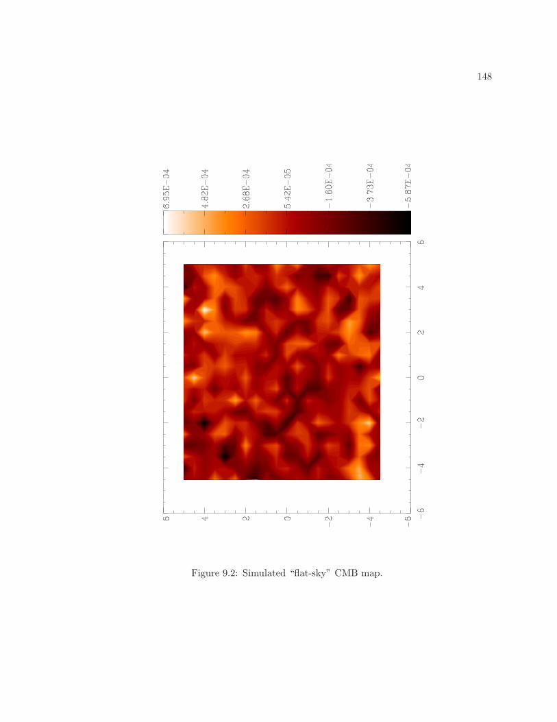
148
Figure 9.2: Simulated “flat-sky” CMB map.
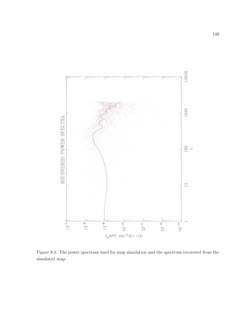
149
Figure 9.3: The power spectrum used for map simulation and the spectrum recovered from the
simulated map.
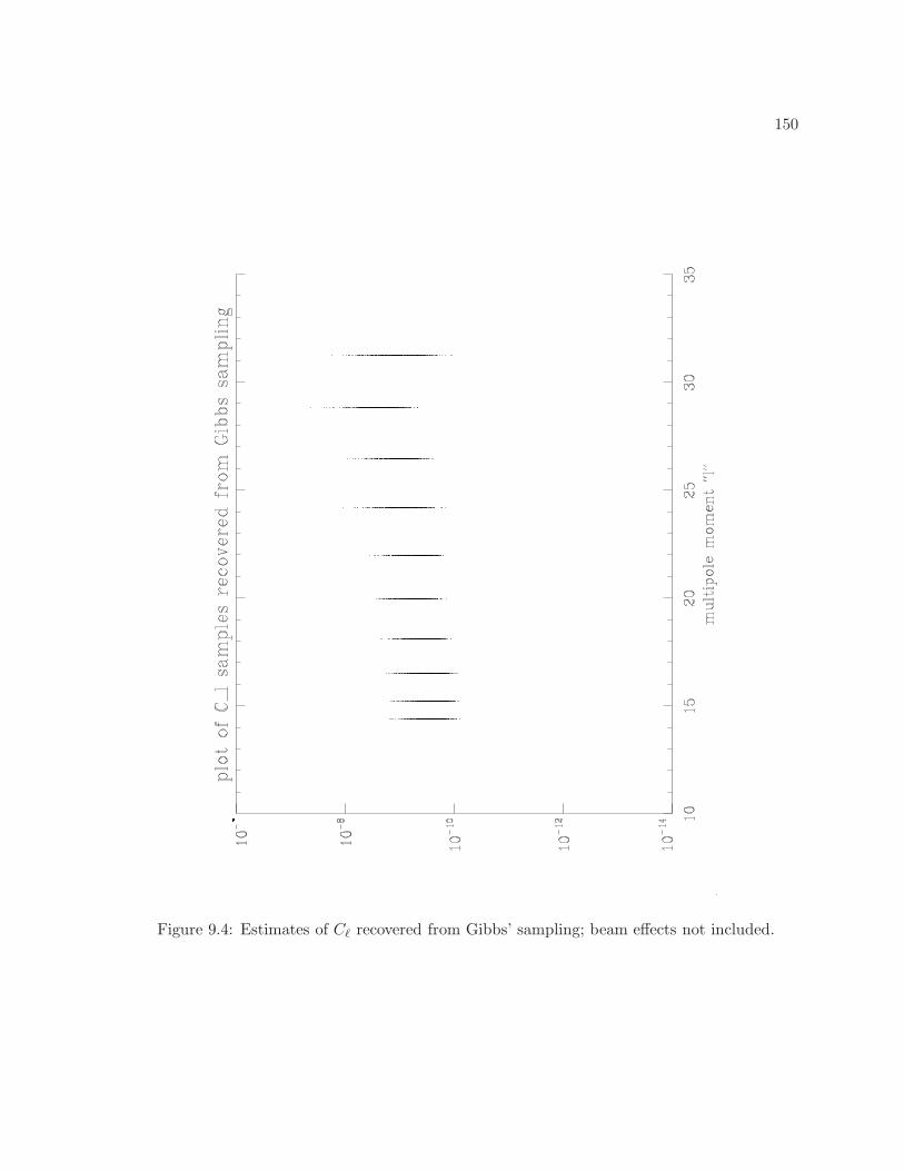
150
Figure 9.4: Estimates of Cℓ recovered from Gibbs’ sampling; beam effects not included.
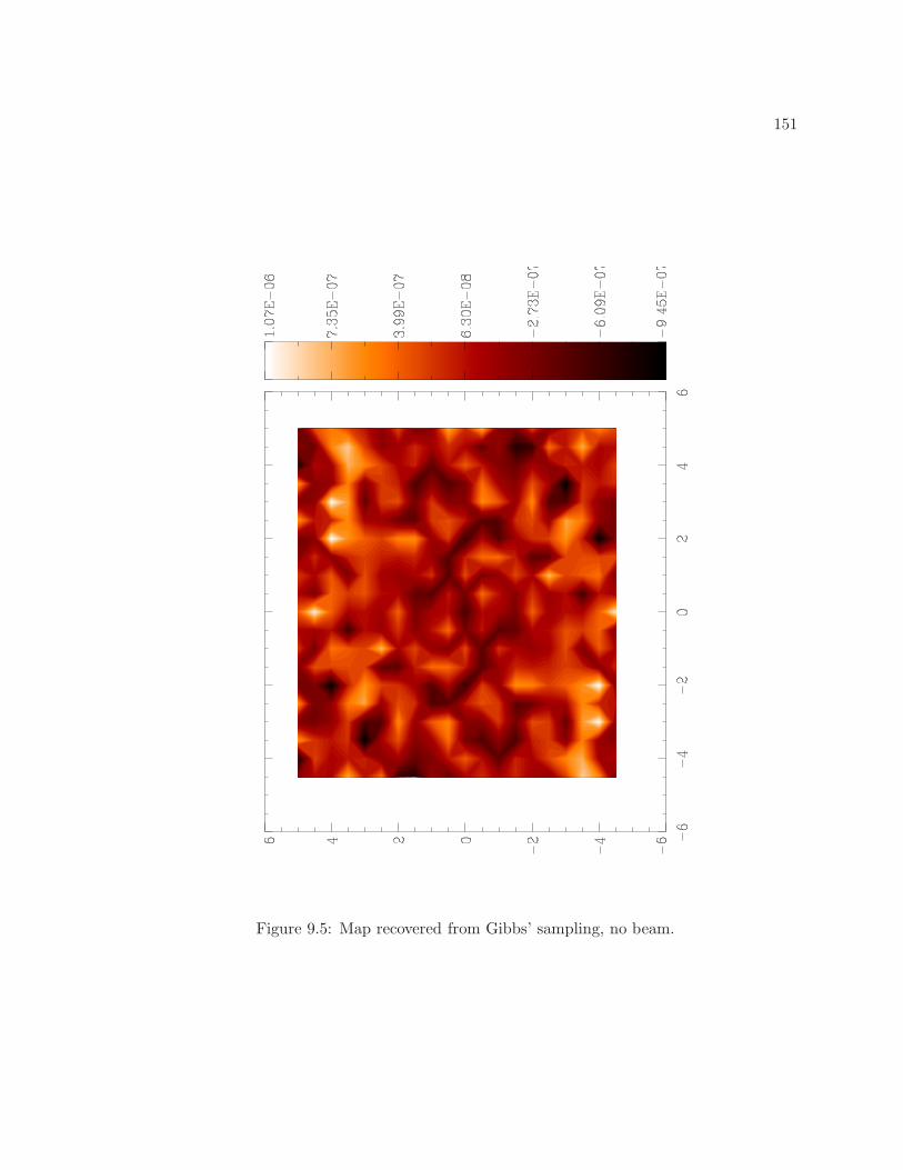
151
Figure 9.5: Map recovered from Gibbs’ sampling, no beam.
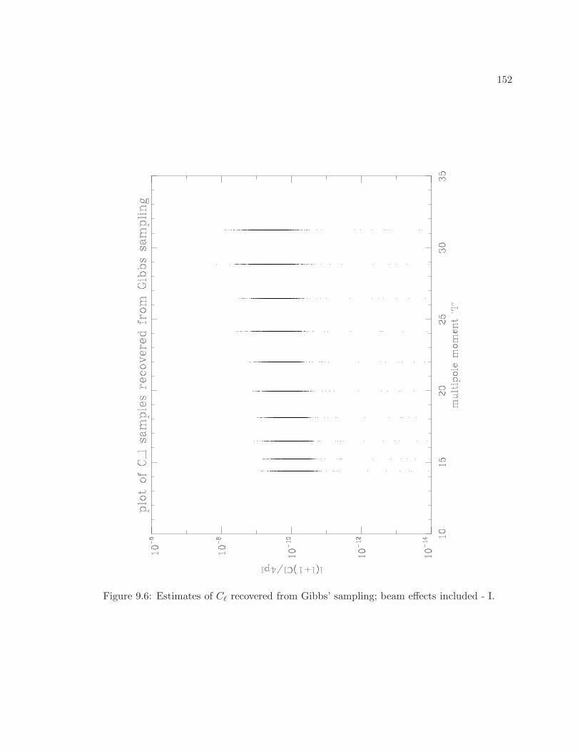
152
Figure 9.6: Estimates of Cℓ recovered from Gibbs’ sampling; beam effects included - I.
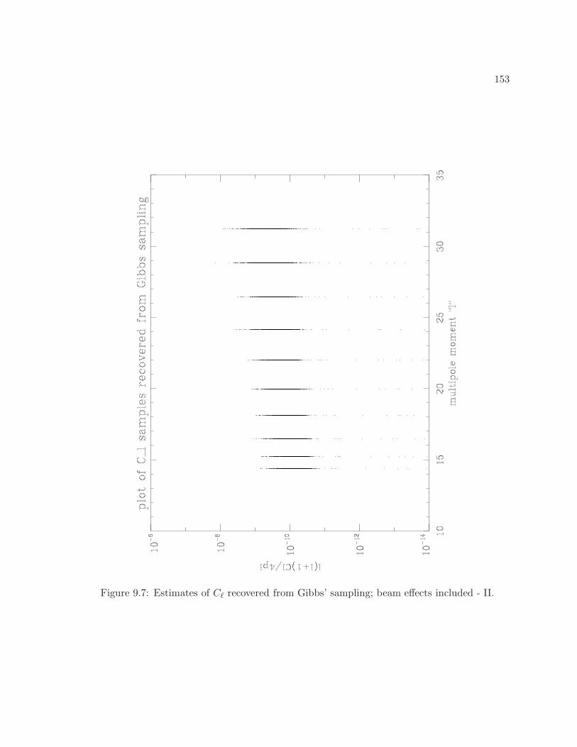
153
Figure 9.7: Estimates of Cℓ recovered from Gibbs’ sampling; beam effects included - II.
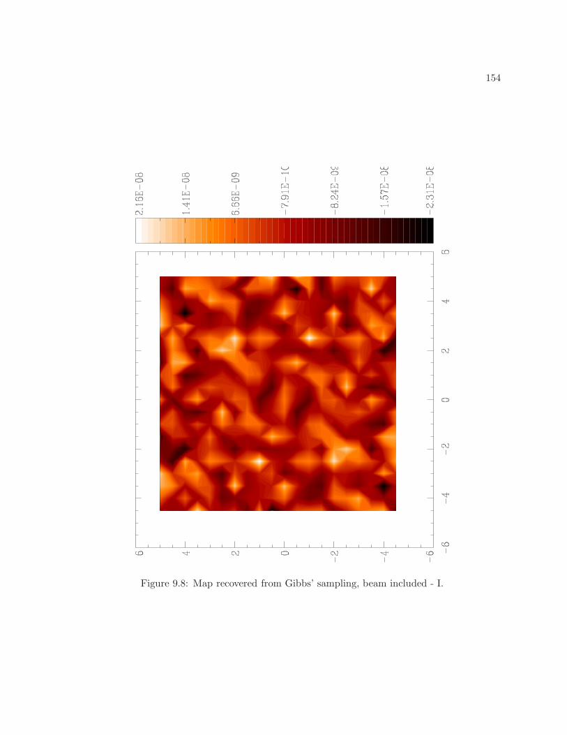
154
Figure 9.8: Map recovered from Gibbs’ sampling, beam included - I.

155
Figure 9.9: Map recovered from Gibbs’ sampling, beam included - II.
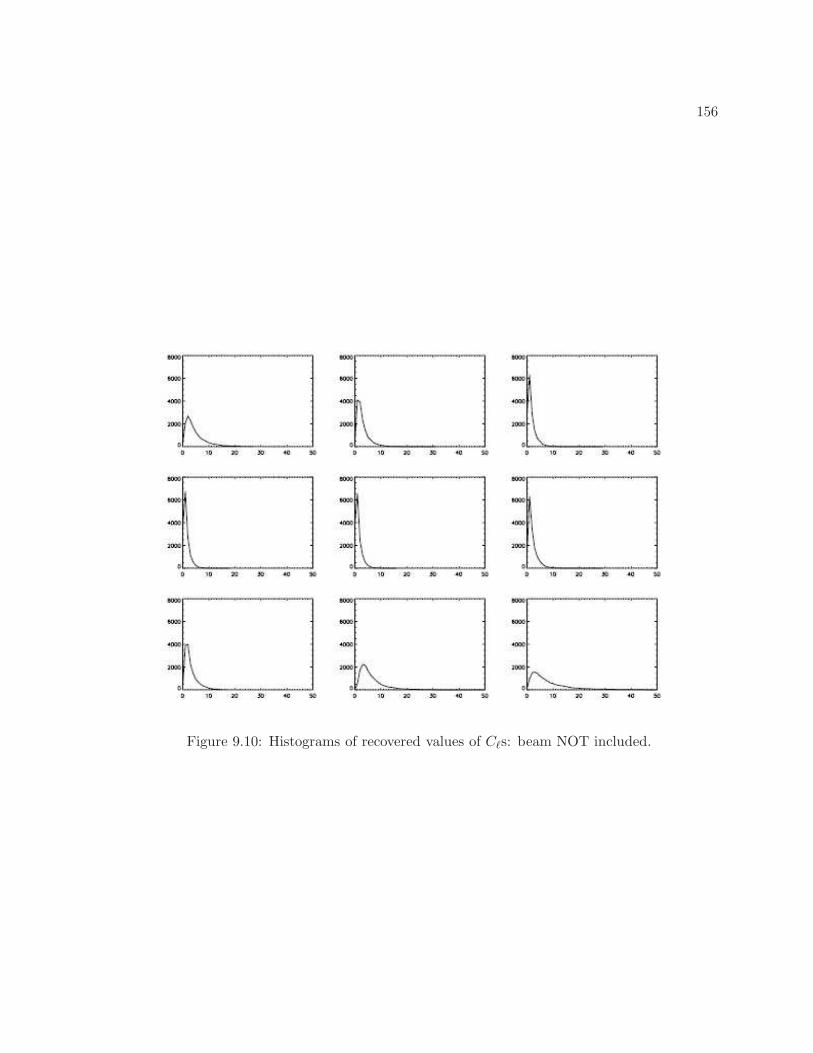
156
Figure 9.10: Histograms of recovered values of Cℓs: beam NOT included.
157
Bibliography
[1] M. Tegmark, “How to Make Maps from Cosmic Microwave Background Data without
Losing Information,” ApJ Lett., vol. 480, pp. L87+, May 1997.
[2] S. Dodelson, Modern cosmology, Modern cosmology / Scott Dodelson. Amsterdam (Nether-
lands): Academic Press. ISBN 0-12-219141-2, 2003, XIII + 440 p., 2003.
[3] B. D. Wandelt, D. L. Larson, and A. Lakshminarayanan, “Global, exact cosmic microwave
background data analysis using Gibbs sampling,” Phys. Rev. D, vol. 70, no. 8, pp. 083511–
+, Oct. 2004.
[4] B. D. Wandelt, “MAGIC: Exact Bayesian Covariance Estimation and Signal Reconstruc-
tion for Gaussian Random Fields,” ArXiv Astrophysics e-prints, Jan. 2004.
[5] J. R. Bond, A. H. Jaffe, and L. Knox, “Estimating the power spectrum of the cosmic
microwave background,” Phys. Rev. D, vol. 57, pp. 2117–2137, Feb. 1998.
[6] M. P. Hobson and K. Maisinger, “Maximum-likelihood estimation of the cosmic microwave
background power spectrum from interferometer observations,” Monthly Notices of the
RAS, vol. 334, pp. 569–588, Aug. 2002.
[7] B. Wandelt and S.S. Malu, “Gibbs’ sampling for Interferometry,” Work in progress, 2007.
[8] Tanner, Tools for Statistical Inference: Methods for the Exploration of Posterior Distribu-
tions and Likelihood Functions, Springer Verlag, Heidelberg, Germany., 1996.
[9] G. Huey, R. H. Cyburt, and B. D. Wandelt, “Precision primordial 4He measurement from
the CMB,” Phys. Rev. D, vol. 69, no. 10, pp. 103503–+, May 2004.
[10] Gelman, Andrew and Rubin, Donald B., “Inference from iterative simulation using multiple
sequences,” Statistical Science, vol. 7, no. 4, pp. 457–472, nov 1992.
158
Chapter 10
Conclusions
In this thesis, we have introduced a novel interferometer, the Millimeter-wave Bolometric Inter-
ferometer, which combines the advantages of interferometry with the sensitivity of bolometers.
Furthermore, MBI has a novel quasi-optical beam-combination arrangement that will allow it
to simultaneously function as an interferometer and an imager. In addition, an efficient sta-
tistical technique already employed by Wandelt et al [1, 2] for imagers was adapted for an
interferometer. Several instrumental aspects were also studied in chapter 5 and two different
measurement/instrument optimization techniques explored (§7.7.1,§7.6,§7.7). These techniques
will provide MBI with the sensitivity required to provide upper limits to B-mode levels. But
MBI-4 has just six baselines and a 7 beam - these parameters imply large pixels in u-v space.
Future versions of MBI and another planned space-based version [3] will have larger beams
(∼15), leading to smaller pixels in the u-v plane. A space-based version (called EPIC) is also
intended to have many more detectors in the focal plane in its Fizeau system. EPIC is also
planned to have several “units”, each in a different bandwidth, each with several dozens of
antennae, providing both the ℓ-space coverage and a means to characterize foregrounds.
This thesis has thus introduced a new kind of instrument with exquisite control over
systematic effects, brought about through instrument optimization. In particular, it can simul-
taneously observe as an imager and an interferometer. Power spectra can thus be computed
with both approaches and compared.
But comparing power spectra is not all. MBI can make images of those parts of the
sky where foregrounds are known to dominate the CMB signal. This same information can
simultaneously be obtained in the u-v plane, split into several sub-bands. This provides us with
the ability to perform a unique comparison of foregrounds and systematic effects in image plane
and the u-v plane. If we add the advantage of several bands to this instrument, we gain the
ability to characterize foregrounds as well as detect the faint B-mode signal. This
is a unique ability, not yet achieved by an experiment in CMB cosmology. This eliminates the

159
need to cross-correlate data from several experiments to eliminate foregrounds, thereby allowing
greater control over instrument systematics. In this sense, the MBI is a complete instrument,
supported by the analysis and simulation techniques developed in this thesis.
160
Bibliography
[1] B. D. Wandelt, D. L. Larson, and A. Lakshminarayanan, “Global, exact cosmic microwave
background data analysis using Gibbs sampling,” Phys. Rev. D, vol. 70, no. 8, pp. 083511–+,
Oct. 2004.
[2] B. D. Wandelt, “MAGIC: Exact Bayesian Covariance Estimation and Signal Reconstruction
for Gaussian Random Fields,” ArXiv Astrophysics e-prints, Jan. 2004.
[3] P. T. Timbie, G. S. Tucker, P. A. R. Ade, S. Ali, E. Bierman, E. F. Bunn, C. Calderon,
A. C. Gault, P. O. Hyland, B. G. Keating, J. Kim, A. Korotkov, S. S. Malu, P. Mauskopf,
J. A. Murphy, C. O’Sullivan, L. Piccirillo, and B. D. Wandelt, “The Einstein polarization
interferometer for cosmology (EPIC) and the millimeter-wave bolometric interferometer
(MBI),” New Astronomy Review, vol. 50, pp. 999–1008, Dec. 2006.
161
Appendix A
Dr. Planck, or: How I Learned to Stop Worrying
and Love Stat Mech.
A.1 The general problem
We wish to figure out how particles are distributed among N states, ni, each with energy
En - this is the general problem that Statistical Mechanics addresses. In these notes we will
restrict ourselves to photons.
In general, the distribution function U (E) is given by U (E) dE = number of available
states × average energy per unit state. The number of available states is usually referred to in
literature as the ‘phase factor’. We must then, deal with two separate calculations.
A.2 Average Energy
For a photon, Eγ = hν. In general, the nth state will have energy En = nhν. To find
the average energy per state, we sum over the entire distribution, weighing each state with a
factor given by the distribution function in this case the Boltzmann distribution function given
by e−βEn where β = 1kT . The average energy then is
E =
∑
nEne
−βEn
∑
ne−βEn
(A.1)
In Statistical Mechanics, the sum∑
ne−βEn is called the Partition function, and all physical
quantities like (average) Energy, Entropy etc. can easily be related to it. Below is a simple
example of such a relation that is useful to us. Call Z the Partition function, so that Z =
162
∑
ne−βEn Then differentiate Z w.r.t. β to get:
∂Z
∂β= −
∑
n
Ene−βEn (A.2)
We immediately see that this is very close to the expression for E above; all we need to do is
to divide this by∑
n e−βEn , which is exactly Z. So we get, adding a minus sign,
E = − 1
Z
∂Z
∂β≡ −∂ lnZ
∂β(A.3)
Now, for photons,
Z =∑
n
e−βEn =
∞∑
n=0
e−βnhν (A.4)
Recall now that ∞∑
n=0
r−nα =1
1− r (A.5)
Applying that here, we get, with r ≡ e−βhν
Z =1
1− e−βhν (A.6)
⇒ lnZ = − ln |1− e−βhν | (A.7)
⇒ E = −∂ lnZ
∂β= +
1
1− e−βhν · −e−βhν · −hν =
hν
(1− e−βhν) eβhν =hν
eβhν − 1(A.8)
A.3 Number of phase states available, or phase factor
The Uncertainty Principle decides the ‘minimum size’ of a ‘phase cell’ because
dxdp ≥ h (A.9)
⇒ d3xd3p ≥ h3 (A.10)
Therefore, given a certain phase-space volume d3xd3p, the number of ‘cells’ available in that
phase space is
ζ =d3xd3p
h3(A.11)
Writing the volume in real space as V , we get
ζ =V d3p
h3=
4πp2dp · Vh3
(A.12)
163
For photons, E = pc from Special Relativity ⇒ p = Ec = hν
c
⇒ ζ = 4π6 h2ν2
c2· 6 hdν
c· 1
6 h3· V =
4π
c3ν2dν · V (A.13)
Now, we account for the fact that there are two unique polarization states possible for any given
direction of propagation. The above expression becomes
ζ =8π
c3ν2dν · V (A.14)
A.4 Planck Distribution
Planck distribution can then be written as a multiple of the two factors in the two sections
above
U (ν) dν =8π
c3ν2 · hν
eβhν − 1dνV (A.15)
We can express the LHS in terms of the energy density instead of energy, so that
u (ν) dν =8π
c3ν2 · hν
eβhν − 1dν (A.16)
This is the expression we wanted.
What we really need in calculations for the MBI, though, are integrals of this functions
× other functions, like the interference pattern on the bolometers. While doing an integral, it
is always very convenient to separate out unitless quantities that we integrate over, and factors
that depend on the physics of the situation. In this case we define a unitless quantity x = hνkT
and strive to present this distribution in terms of x thus:
u (ν) dν =8π
c3
(hν
kT
)2
·(kT
h
)2
·(hν
kT
)
· kT(
1
ehνkT − 1
)
d
(hν
kT
)(kT
h
)
(A.17)
Replacing hνkT by x, and collecting all other factors together, we get
u (ν) dν =8πh
c3
(kT
h
)4 x3
ex − 1dx (A.18)
where u has units JHz−1m−3, i.e. energy per unit volume per unit frequency interval. But the
energy radiated out in all directions is the same. Moreover, we are interested in the spectral
intensity, i.e. power per unit area per unit solid angle per unit frequency integral. We denote
the spectral intensity by I, and this is how I is related to u:
I (ν, T ) =u (ν, T ) c
4π(A.19)
such that
I (ν, T ) =2h
c2
(kT
h
)4 x3
ex − 1dx (A.20)
164
We can also write this as
I (ν, T ) = Bν (T ) dν (A.21)
for a black body, where
Bν =2hν3
c2(ex − 1)−1 [Wm−2Sr−1Hx−1
](A.22)
so that
I (ν, T ) =2hν3
c2(ex − 1)−1 dν
[Wm−2Sr−1
](A.23)
However, if the signal varies across the sky, then Bν is a function of (θ, φ). Thus, if we write
T = T0 + δT (θ, φ) (A.24)
for the CMB, then
Bν (T + δT ) = Bν (T0) +∂B
∂TδT ≡ Bν (T0) + ∆B (A.25)
If we are studying the anisotropies in the CMB, we are interested only in the second term,
which we can write as∂B
∂x
∂x
∂(
1T
)∂(
1T
)
∂T=
2kν2
c2x2ex
(ex − 1)2(A.26)
so that
∆B (θ, φ) =2k
λ2
(x2ex
(ex − 1)2
)
δT (θ, φ) (A.27)
Multiply and divide by hkT0
(in order to end up with dx instead of dν in the expression for
intensity, I):
∆B (θ, φ) =2k2T0
hλ2
(x2ex
(ex − 1)2
)
δT (θ, φ)
(h
kT0
)[Wm−2Sr−1Hz−1
](A.28)
Now, because of the extra factor of hkT0
at the end, we can write the intensity as
∆I (θ, φ) =2k2T0
hλ2
(x2ex
(ex − 1)2
)
δT (θ, φ) dx[Wm−2Sr−1
](A.29)
This is the quantity that we wish to calculate in the instrument simulation, given a simulated
map of the sky.
165
A.5 Distribution for particle number
We can follow through §A.2 for number of particles too. Similar to eq(A.1), we can write
n =
∑
nne−βEn
∑
ne−βEn
(A.30)
Recall that En = nhν, so that1
hν
∂Z
∂β= −
∑
n
ne−βEn (A.31)
and we can write
n =E
hν= − 1
hν
1
Z
∂Z
∂β≡ − 1
hν
∂ lnZ
∂β=
1
eβhν − 1(A.32)
Using the phase space factor from §A.3, we get that the number of particles between ν and
ν + dν, given by n (ν) dν is
n (ν) dν =8π
c3ν2
eβhν − 1dν (A.33)
The author is forever indebted to late Dr. Swaminathan for his expositions on Statistical
Mechanics.
166
Appendix B
S- and T-matrix formulation
B.1 Two port devices and the S-matrix
Most of the microwave devices we use in our lab are 2-port devices, and are usually used
in series, e.g. a w/g twist with a w/g straight piece. Any 2-port device has two possible inputs
and two outputs. We label the inputs with a and outputs with b.
For all practical purposes, we are interested not in the values of the outputs b, but what
they are compared to the inputs. In other words, we wish to look at the generic ratios
output
input(B.1)
for all four quantities.
The most simple-minded approach would be to define the four ratios b1a1
etc., but we can
write these out systematically as:
b1 = S11a1 + S12a2 (B.2)
b2 = S21a1 + S22a2 (B.3)
The above equations can also be in vector form written as:
~b = ~S · ~a (B.4)
or, better still, in matrix form, which is more useful for our purpose:[
b1
b2
]
=
[
S11 S12
S21 S22
][
a1
a2
]
(B.5)
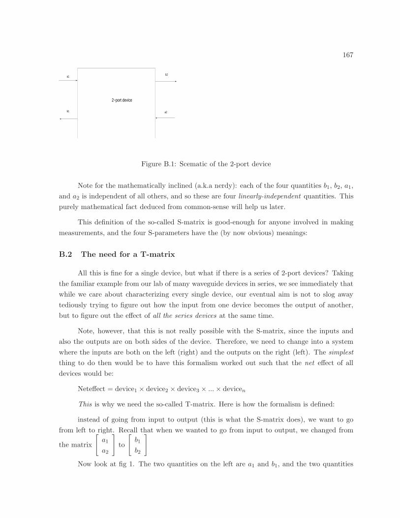
167
b1 a2
b2a1
2−port device
Figure B.1: Scematic of the 2-port device
Note for the mathematically inclined (a.k.a nerdy): each of the four quantities b1, b2, a1,
and a2 is independent of all others, and so these are four linearly-independent quantities. This
purely mathematical fact deduced from common-sense will help us later.
This definition of the so-called S-matrix is good-enough for anyone involved in making
measurements, and the four S-parameters have the (by now obvious) meanings:
B.2 The need for a T-matrix
All this is fine for a single device, but what if there is a series of 2-port devices? Taking
the familiar example from our lab of many waveguide devices in series, we see immediately that
while we care about characterizing every single device, our eventual aim is not to slog away
tediously trying to figure out how the input from one device becomes the output of another,
but to figure out the effect of all the series devices at the same time.
Note, however, that this is not really possible with the S-matrix, since the inputs and
also the outputs are on both sides of the device. Therefore, we need to change into a system
where the inputs are both on the left (right) and the outputs on the right (left). The simplest
thing to do then would be to have this formalism worked out such that the net effect of all
devices would be:
Neteffect = device1 × device2 × device3 × ...× devicen
This is why we need the so-called T-matrix. Here is how the formalism is defined:
instead of going from input to output (this is what the S-matrix does), we want to go
from left to right. Recall that when we wanted to go from input to output, we changed from
the matrix
[
a1
a2
]
to
[
b1
b2
]
Now look at fig 1. The two quantities on the left are a1 and b1, and the two quantities
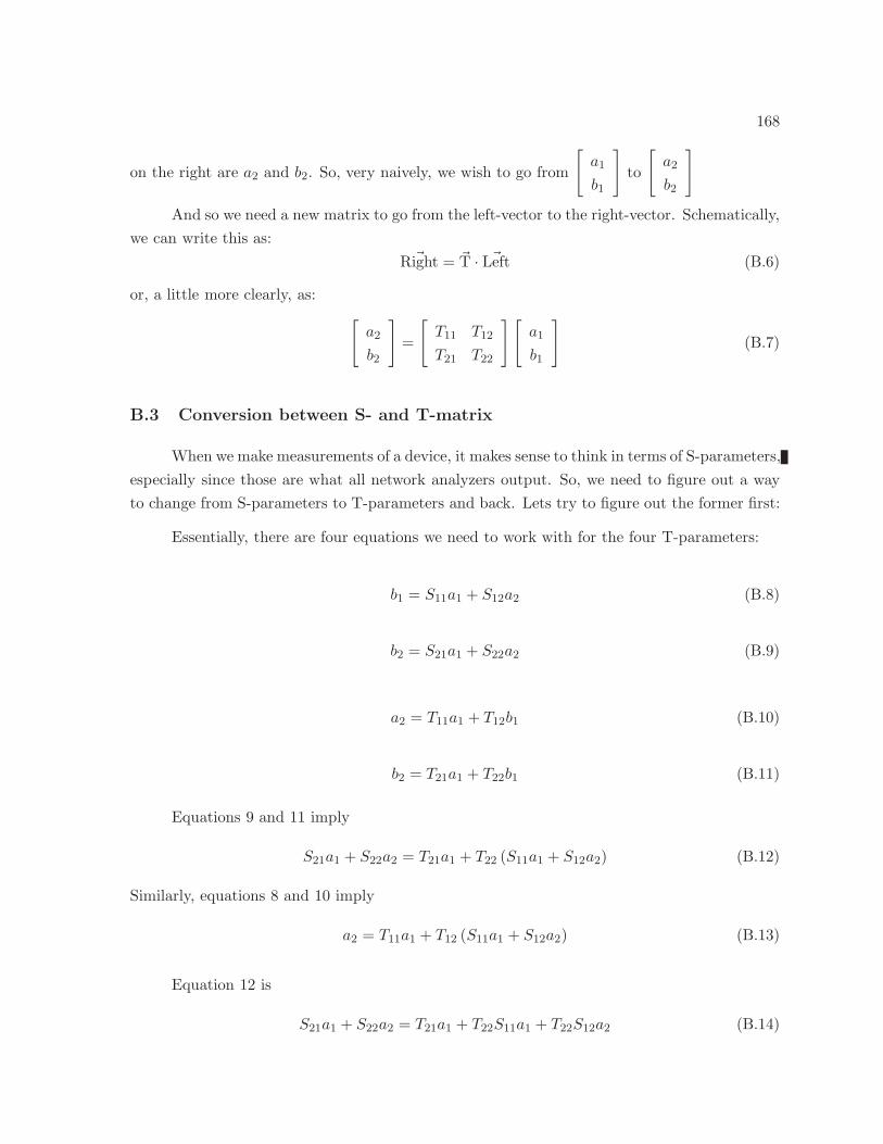
168
on the right are a2 and b2. So, very naively, we wish to go from
[
a1
b1
]
to
[
a2
b2
]
And so we need a new matrix to go from the left-vector to the right-vector. Schematically,
we can write this as:~Right = ~T · ~Left (B.6)
or, a little more clearly, as:
[
a2
b2
]
=
[
T11 T12
T21 T22
][
a1
b1
]
(B.7)
B.3 Conversion between S- and T-matrix
When we make measurements of a device, it makes sense to think in terms of S-parameters,
especially since those are what all network analyzers output. So, we need to figure out a way
to change from S-parameters to T-parameters and back. Lets try to figure out the former first:
Essentially, there are four equations we need to work with for the four T-parameters:
b1 = S11a1 + S12a2 (B.8)
b2 = S21a1 + S22a2 (B.9)
a2 = T11a1 + T12b1 (B.10)
b2 = T21a1 + T22b1 (B.11)
Equations 9 and 11 imply
S21a1 + S22a2 = T21a1 + T22 (S11a1 + S12a2) (B.12)
Similarly, equations 8 and 10 imply
a2 = T11a1 + T12 (S11a1 + S12a2) (B.13)
Equation 12 is
S21a1 + S22a2 = T21a1 + T22S11a1 + T22S12a2 (B.14)
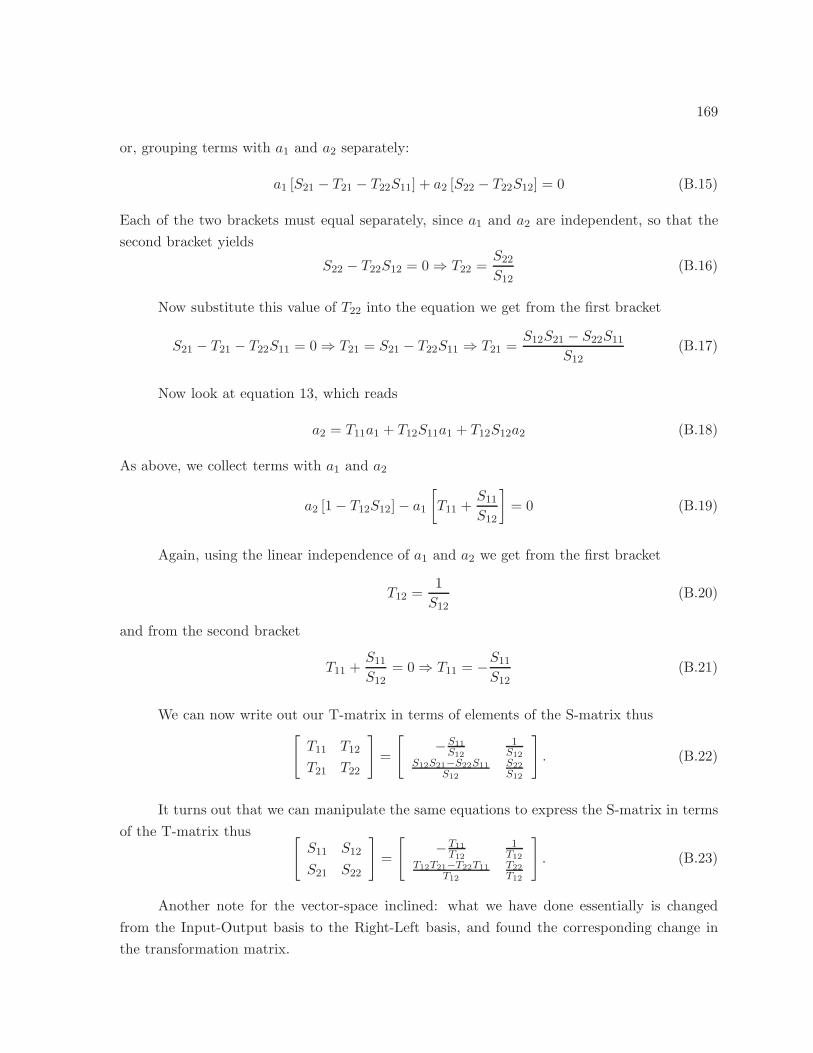
169
or, grouping terms with a1 and a2 separately:
a1 [S21 − T21 − T22S11] + a2 [S22 − T22S12] = 0 (B.15)
Each of the two brackets must equal separately, since a1 and a2 are independent, so that the
second bracket yields
S22 − T22S12 = 0⇒ T22 =S22
S12(B.16)
Now substitute this value of T22 into the equation we get from the first bracket
S21 − T21 − T22S11 = 0⇒ T21 = S21 − T22S11 ⇒ T21 =S12S21 − S22S11
S12(B.17)
Now look at equation 13, which reads
a2 = T11a1 + T12S11a1 + T12S12a2 (B.18)
As above, we collect terms with a1 and a2
a2 [1− T12S12]− a1
[
T11 +S11
S12
]
= 0 (B.19)
Again, using the linear independence of a1 and a2 we get from the first bracket
T12 =1
S12(B.20)
and from the second bracket
T11 +S11
S12= 0⇒ T11 = −S11
S12(B.21)
We can now write out our T-matrix in terms of elements of the S-matrix thus[
T11 T12
T21 T22
]
=
[
−S11
S12
1S12
S12S21−S22S11
S12
S22
S12
]
. (B.22)
It turns out that we can manipulate the same equations to express the S-matrix in terms
of the T-matrix thus [
S11 S12
S21 S22
]
=
[
−T11
T12
1T12
T12T21−T22T11
T12
T22
T12
]
. (B.23)
Another note for the vector-space inclined: what we have done essentially is changed
from the Input-Output basis to the Right-Left basis, and found the corresponding change in
the transformation matrix.
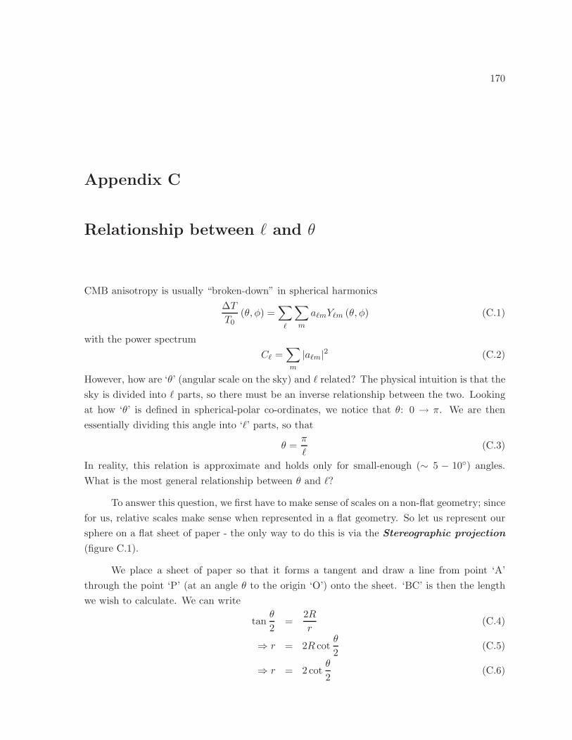
170
Appendix C
Relationship between ℓ and θ
CMB anisotropy is usually “broken-down” in spherical harmonics
∆T
T0(θ, φ) =
∑
ℓ
∑
m
aℓmYℓm (θ, φ) (C.1)
with the power spectrum
Cℓ =∑
m
|aℓm|2 (C.2)
However, how are ‘θ’ (angular scale on the sky) and ℓ related? The physical intuition is that the
sky is divided into ℓ parts, so there must be an inverse relationship between the two. Looking
at how ‘θ’ is defined in spherical-polar co-ordinates, we notice that θ: 0 → π. We are then
essentially dividing this angle into ‘ℓ’ parts, so that
θ =π
ℓ(C.3)
In reality, this relation is approximate and holds only for small-enough (∼ 5 − 10) angles.
What is the most general relationship between θ and ℓ?
To answer this question, we first have to make sense of scales on a non-flat geometry; since
for us, relative scales make sense when represented in a flat geometry. So let us represent our
sphere on a flat sheet of paper - the only way to do this is via the Stereographic projection
(figure C.1).
We place a sheet of paper so that it forms a tangent and draw a line from point ‘A’
through the point ‘P’ (at an angle θ to the origin ‘O’) onto the sheet. ‘BC’ is then the length
we wish to calculate. We can write
tanθ
2=
2R
r(C.4)
⇒ r = 2R cotθ
2(C.5)
⇒ r = 2cotθ
2(C.6)
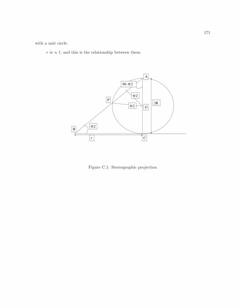
171
with a unit circle.
r is ∝ ℓ, and this is the relationship between them.
R
r
P
B
C
O
A
Figure C.1: Stereographic projection
172
Appendix D
Inflaton field equation of motion and slow-roll
conditions
This is my attempt to heuristically ‘derive’ the inflaton-field equation of motion (which is fairly
straightforward) and the slow-roll conditions, which every set of notes or book/s define/quote in
their own way. Fed up of the lack of consensus in literature, I attempt to follow the convention
that makes most sense to me. Usual health warnings apply: this is my attempt at understanding
these topics, so I make no claim about these notes being right.
D.1 The equation of motion
Let us start from the first law of thermodynamics:
dU + pdV = 0 (D.1)
where, naturally, U = ρa3, where ρ is the density (total energy density, but since we are in
the inflation-era, ρ is dominated by the energy density of the inflaton field φ) and a the scale
factor, which is a function of time.
Substituting for U , we get
a3dρ+ 3a2daρ+ 3a2dap = 0 (D.2)
⇒ 3a2 (p+ ρ) = −a3dρ (D.3)
Now, for a field, we have the following expressions for pressure and energy density:
ρ = KE + PE =1
2
(dφ
dt
)2
+ V (φ) (D.4)
173
p = KE − PE =1
2
(dφ
dt
)2
− V (φ) (D.5)
where the second equation can be derived from the general expression for the energy-momentum
tensor. See, for instance, [1]. From these two expressions, we get
p+ ρ =
(dφ
dt
)2
(D.6)
which we can now substitute in eq. 3 to get:
3a2
(dφ
dt
)2
da = −a3dρ (D.7)
⇒ dρ
da= −3
a
(dφ
dt
)2
(D.8)
Now, if we differentiate the expression for ρ w.r.t. time, we get
dρ
dt=dφ
dt
d2ρ
dt2+dV
dφ
dφ
dt(D.9)
But dρdt = dρ
dadadt , so the above equation becomes, after substituting for dρ
da
−3
a
da
dt
(dφ
dt
)2
=dφ
dt
d2φ
dt2+dV
dφ
dφ
dt(D.10)
After cancelling dφdt from every term,
−31
a
da
dt
dφ
dt=d2φ
dt2+dV
dφ(D.11)
But 1adadt is H, the Hubble paramter, so that
d2φ
dt2+ 3H
dφ
dt+dV
dφ= 0 (D.12)
This, then, is the equation of motion.
Let us now slip into a more comfortable notation: dφdt ≡ φ and dV
dφ ≡ V ′. The equation of
motion is
φ+ 3Hφ+ V ′ = 0 (D.13)
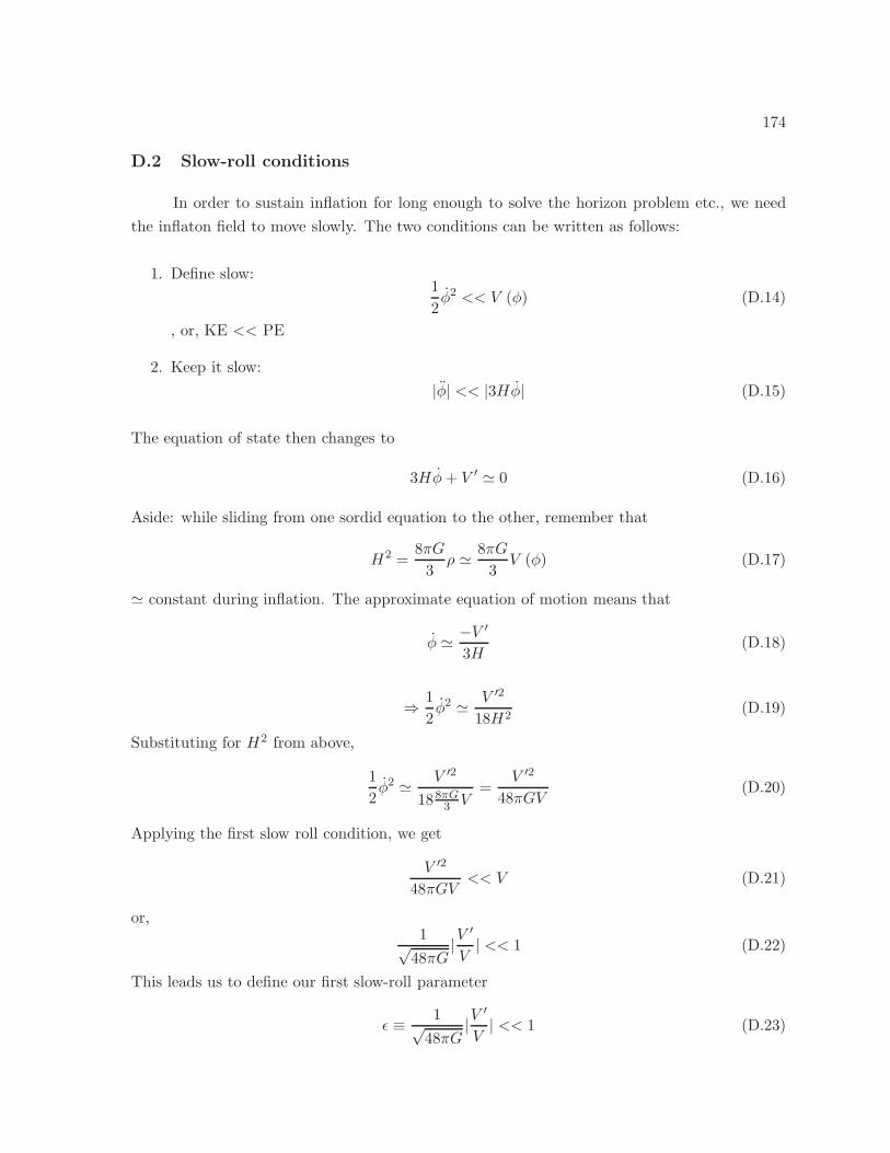
174
D.2 Slow-roll conditions
In order to sustain inflation for long enough to solve the horizon problem etc., we need
the inflaton field to move slowly. The two conditions can be written as follows:
1. Define slow:1
2φ2 << V (φ) (D.14)
, or, KE << PE
2. Keep it slow:
|φ| << |3Hφ| (D.15)
The equation of state then changes to
3Hφ+ V ′ ≃ 0 (D.16)
Aside: while sliding from one sordid equation to the other, remember that
H2 =8πG
3ρ ≃ 8πG
3V (φ) (D.17)
≃ constant during inflation. The approximate equation of motion means that
φ ≃ −V′
3H(D.18)
⇒ 1
2φ2 ≃ V ′2
18H2(D.19)
Substituting for H2 from above,
1
2φ2 ≃ V ′2
188πG3 V
=V ′2
48πGV(D.20)
Applying the first slow roll condition, we get
V ′2
48πGV<< V (D.21)
or,1√
48πG|V
′
V| << 1 (D.22)
This leads us to define our first slow-roll parameter
ǫ ≡ 1√48πG
|V′
V| << 1 (D.23)
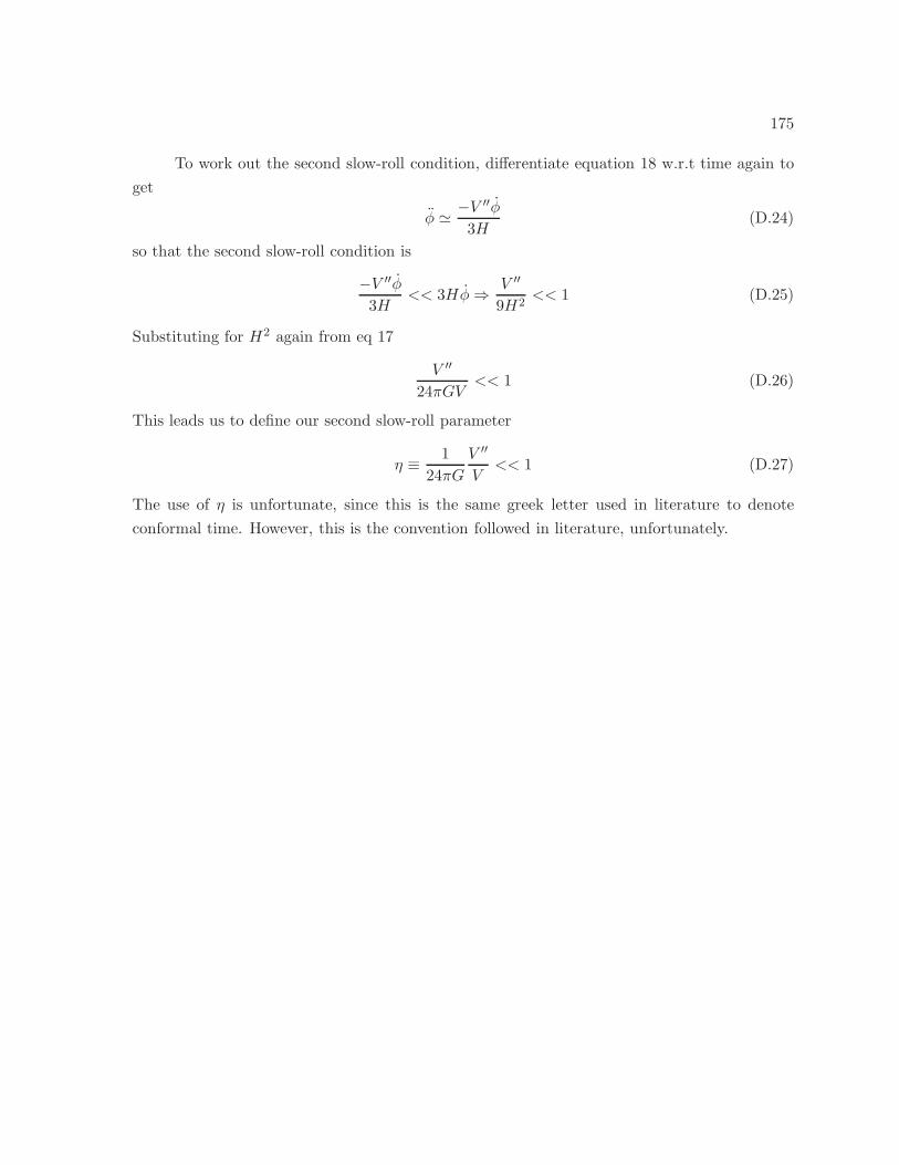
175
To work out the second slow-roll condition, differentiate equation 18 w.r.t time again to
get
φ ≃ −V′′φ
3H(D.24)
so that the second slow-roll condition is
−V ′′φ3H
<< 3Hφ⇒ V ′′
9H2<< 1 (D.25)
Substituting for H2 again from eq 17
V ′′
24πGV<< 1 (D.26)
This leads us to define our second slow-roll parameter
η ≡ 1
24πG
V ′′
V<< 1 (D.27)
The use of η is unfortunate, since this is the same greek letter used in literature to denote
conformal time. However, this is the convention followed in literature, unfortunately.
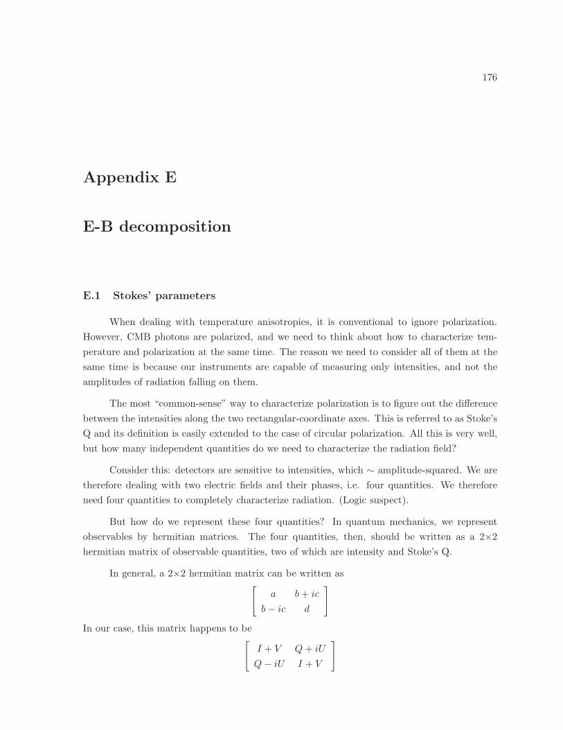
176
Appendix E
E-B decomposition
E.1 Stokes’ parameters
When dealing with temperature anisotropies, it is conventional to ignore polarization.
However, CMB photons are polarized, and we need to think about how to characterize tem-
perature and polarization at the same time. The reason we need to consider all of them at the
same time is because our instruments are capable of measuring only intensities, and not the
amplitudes of radiation falling on them.
The most “common-sense” way to characterize polarization is to figure out the difference
between the intensities along the two rectangular-coordinate axes. This is referred to as Stoke’s
Q and its definition is easily extended to the case of circular polarization. All this is very well,
but how many independent quantities do we need to characterize the radiation field?
Consider this: detectors are sensitive to intensities, which ∼ amplitude-squared. We are
therefore dealing with two electric fields and their phases, i.e. four quantities. We therefore
need four quantities to completely characterize radiation. (Logic suspect).
But how do we represent these four quantities? In quantum mechanics, we represent
observables by hermitian matrices. The four quantities, then, should be written as a 2×2
hermitian matrix of observable quantities, two of which are intensity and Stoke’s Q.
In general, a 2×2 hermitian matrix can be written as[
a b+ ic
b− ic d
]
In our case, this matrix happens to be[
I + V Q+ iU
Q− iU I + V
]
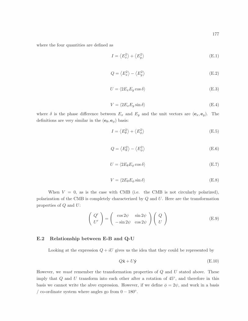
177
where the four quantities are defined as
I =⟨E2x
⟩+⟨E2y
⟩(E.1)
Q =⟨E2x
⟩−⟨E2y
⟩(E.2)
U = 〈2ExEy cos δ〉 (E.3)
V = 〈2ExEy sin δ〉 (E.4)
where δ is the phase difference between Ex and Ey and the unit vectors are (ex, ey). The
definitions are very similar in the (eθ, eφ) basis:
I =⟨E2θ
⟩+⟨E2φ
⟩(E.5)
Q =⟨E2θ
⟩−⟨E2φ
⟩(E.6)
U = 〈2EθEφ cos δ〉 (E.7)
V = 〈2EθEφ sin δ〉 (E.8)
When V = 0, as is the case with CMB (i.e. the CMB is not circularly polarized),
polarization of the CMB is completely characterized by Q and U . Here are the transformation
properties of Q and U :
(
Q′
U ′
)
=
(
cos 2ψ sin 2ψ
− sin 2ψ cos 2ψ
)(
Q
U
)
(E.9)
E.2 Relationship between E-B and Q-U
Looking at the expression Q+ iU gives us the idea that they could be represented by
Qx + U y (E.10)
However, we must remember the transformation properties of Q and U stated above. These
imply that Q and U transform into each other after a rotation of 45, and therefore in this
basis we cannot write the abve expression. However, if we define φ = 2ψ, and work in a basis
/ co-ordinate system where angles go from 0− 180.
178
We can now proceed with the math of E-B decomposition. In very simple terms, what
we want is to split both Q and U into a gradient component and a curl component. But that
is easily done, for any vector field can be written as a sum of the two. For an arbitrary vector
field A, we write
A = ∇ · f +∇×B ≡ G + C (E.11)
where f is a scalar field and B is a vector field, and G and C are the gradient and curl components
of A respectively. Using vector calculus identities, we get
∇ ·A = ∇ · G (E.12)
∇×A = ∇× C (E.13)
Substitute Qx + U y for A and E and B for G and C respectively, we get
∇ ·E = ∇ · (Qx + U y) (E.14)
∇×B = ∇× (Qx + U y) (E.15)
We cannot really do very much else in real space, so lets take the fourier transform of the first
equation, changing all derivatives to factors of l, and take the ∇ out of the integral:
∇ ·∫
d2xEeil·r = ∇ ·∫
d2x (Qx + U y) eil·r (E.16)
Remember the definition of ∇:
∇ =∂
∂xx +
∂
∂yy (E.17)
and with r = xx + yy we get
∫
d2x
(∂
∂xx +
∂
∂yy
)
· eil(cos(xφ)+sin(yφ)) =
∫
d2x
(∂
∂xx +
∂
∂yy
)
· eil(cos(xφ)+sin(yφ))Qx + U y
(E.18)
But(∂
∂xx +
∂
∂yy
)
eil(cos(xφ)+sin(yφ)) = il (cosφx + sinφy) eil(cos(xφ)+sin(yφ)) (E.19)
⇒6 i 6 l∫
d2x (cosφx + sinφy) ·Eeil·r = 6 i 6 l∫
d2x (cosφx + sinφy) · (Qx + U y) eil·r (E.20)
⇒∫
d2xEeil·r =
∫
d2x (Q cosφ+ U sinφ) eil·r (E.21)

179
Denoting fourier transforms like this: E, we get:
E = Q cosφ+ U sinφ (E.22)
Now restore φ = 2ψ:
E = Q cos 2ψ + U sin 2ψ (E.23)
Similarly, for B, we get:
B = −Q sin 2ψ + U cos 2ψ (E.24)

Index
baseline, 41
bolometer, 82
FOV, 37
Gaussianity, 99
last scattering, 26–28
MBI
Instrument, 79
instrument, 82, 98
interferometry, 37
Mutual Coherence Function, 38
North Celestial Pole(NCP), 98
Pine Bluff Observing Site, 81
Power Spectrum, 26
polarized, 26
recombination, 27
Thomson Scattering, 26
Visibility, 42
180


![Compact Mach-Zehnder interferometer based on …MZI implies a millimeter scale footprint of the device, which is a serious disadvantage for integration in micro-processors [3]. Therefore,](https://img.pdfslide.net/doc/110x75/5f756f1f49be326f9f4c28dd/compact-mach-zehnder-interferometer-based-on-mzi-implies-a-millimeter-scale-footprint.jpg)