Fe

dera

l Res

erve

Ban

k of

Chi

cago

The Minimum Wage, Restaurant Prices, and Labor Market Structure Daniel Aaronson, Eric French, and James MacDonald

REVISED August 3, 2007

WP 2004-21

The Minimum Wage, Restaurant Prices, and

Labor Market Structure

Daniel Aaronson, Eric French, and James MacDonald∗

August 3, 2007

Abstract

Using store-level and aggregated Consumer Price Index data, we show that restau-

rant prices rise in response to minimum wage increases under several sources of identifying

variation. We introduce a general model of employment determination that implies min-

imum wage hikes cause prices to rise in competitive labor markets but potentially fall in

monopsonistic environments. Furthermore, the model implies employment and prices are

always negatively related. Therefore, our empirical results provide evidence against the

importance of monopsony power for understanding small observed employment responses

to minimum wage changes. Our estimated price responses challenge other explanations

of the small employment response too.

∗Comments welcome at efrench@frbchi.org or daaronson@frbchi.org. Author affiliations are FederalReserve Bank of Chicago, Federal Reserve Bank of Chicago, and Economic Research Service, U.S. Depart-ment of Agriculture respectively. Work on the store-level price data was performed under a memorandum ofunderstanding between the Economic Research Service at the Department of Agriculture and the Bureau ofLabor Statistics (BLS), which permitted onsite access to the confidential BLS data used in this paper. Wethank Bill Cook, Mark Bowman, and Scott Pinkerton of the BLS for their advice and help. We also thankGadi Barlevy, Jeff Campbell, William Evans (the editor), Bob LaLonde, Derek Neal, Dan Sullivan, the refer-ees, and seminar participants at the Federal Reserve Bank of Chicago, the University of Illinois-Urbana, theEconometric Society, and SOLE meetings for helpful comments and Tina Lam for excellent research assistance.The views expressed herein are not necessarily those of the Federal Reserve Bank of Chicago, Federal ReserveSystem, Bureau of Labor Statistics, or U.S. Department of Agriculture. Author correspondence to DanielAaronson or Eric French, Federal Reserve Bank of Chicago, 230 S. LaSalle St., Chicago, IL 60604. Telephone(312)322-6831, Fax (312)322-2357.

1

1 Introduction

This paper utilizes unique data to test whether restaurant prices respond to minimum

wage changes. We find that restaurant prices unambiguously rise after minimum wage in-

creases are enacted.1 Furthermore, these price increases are larger for establishments that are

more likely to pay the minimum wage. These results are derived from a panel of store-level

restaurant prices that are the basis for the food away from home component of the Consumer

Price Index (CPI) during a three-year period with two Federal minimum wage increases, and

are corroborated using a longer panel of city-level food away from home pricing from the

CPI.

Because of the breadth of our price data, we can take advantage of several sources of

variation. First, some states set their minimum wage above the Federal level. Second, we can

distinguish restaurants that tend to pay the minimum wage from those that do not. Third,

the fraction of workers paid at or near the minimum wage varies across geographic areas. All

three sources of variation indicate that most, if not all, of the higher labor costs faced by

employers are pushed onto customers in the form of higher prices.

As suggested by Brown (1999), the size and sign of these price responses can be used

to infer whether monopsony power is important for understanding the employment response

to minimum wage hikes. The minimum wage literature has become contentious since Card

and Krueger’s (e.g. 1995, 2000) research found that an increase in the minimum wage has

no, or even a small positive, effect on employment. Therefore, their research contradicts

standard models of competitive labor markets, which, prior to their work, most researchers

suspected was relevant for industries which primarily employed minimum wage workers.2

1We are not the first to estimate price pass-through in this context. See, e.g., Converse et al (1981),Card and Krueger (1995), and Aaronson (2001). Card and Krueger use Consumer Price Indices for FoodAway from Home in 27 large metropolitan areas over a three year period, finding larger price increases inthose cities with higher proportions of low-wage workers. Although their estimates are consistent with fullpass-through, their standard errors are extremely large. They cannot reject zero price pass-through in manyof their specifications. Moreover, additional evidence from specific state increases in Texas and New Jerseysuggests close to no price response. As a result, they conclude that their estimates are “too imprecise to reacha more confident assessment about the effects of the minimum wage on restaurant prices.” The size of thepanel that we use in this study allows us to estimate price effects much more precisely.

2See, for example, Brown et al (1982). The standard competitive model’s predictions are generally consis-tent with recent views reported in a survey of leading labor economists (Fuchs, Krueger, and Poterba 1998)as well. However, a full quarter of respondents believe there is no teenage disemployment effect from a 10percent increase in the minimum wage.

2

However, their results are consistent with monopsony power in the labor market, as Stigler

(1946) discussed many years ago. The diverse findings reported in the flurry of replies to

their work (e.g. Neumark and Wascher (1996, 2000), Deere et al. (1995), Kim and Taylor

(1995), Burkhauser et al. (2000), Dickens et al (1999)) led one observer to note that “[Card

and Krueger’s] lasting contribution may well be to show that we just don’t know how many

jobs would be lost if the minimum wage were increased...and that we are unlikely to find

out by using more sophisticated methods of inference on the existing body of data. What is

needed is more sophisticated data” (Kennan 1995).

Restaurant prices complement the existing evidence on employment responses because,

as we show below, output prices and employment are unambiguously negatively related in re-

sponse to an exogenous change in wage rates. In order to show this relationship, we introduce

a general model of employment determination that allows for a range of output and input

market structures. Part of the reasoning behind the negative relationship between output

prices and employment is based on the negative relationship between prices and output. We

also add some weak assumptions to the model to show that output and labor input are posi-

tively related. Therefore, if the output price rises in response to a minimum wage hike, both

output and labor input have fallen. This will be the case if labor markets are competitive.

Conversely, if the output price falls in response to a minimum wage hike, total output and

labor input have increased. This will potentially be the case if firms have monopsony power

in the labor market.

Research on monopsony power has recently been revitalized by the empirical and theo-

retical work of Card and Krueger (1995), Burdett and Mortenson (1998), Bashkar and To

(1999), Ahn and Arcidiacono (2003), Flinn (2006), Manning (1995), and Rebitzer and Taylor

(1995).3 But our results suggest that competition is likely more relevant than monopsony.

Moreover, in Aaronson and French (2007), we show that a computational model of labor

demand with a competitive labor market structure predicts price responses that are compa-

rable to those found in this paper. The employment elasticities that are derived from that

3Although few believe that low wage labor markets are characterized by pure monopsony, as in Stigler(1946), many models give rise to monopsony-like behavior that corroborate Card and Krueger’s findings ofsmall or even positive employment movements after a minimum wage increase. These include models wheretransportation (Bashkar and To 1999) or employee search (Burdett and Mortenson 1998; Ahn and Arcidiacono2003; Flinn 2006) is costly and employers are not able to discriminate high and low reservation wage workers.Efficiency wage models such as Manning (1995) and Rebitzer and Taylor (1995) can also cause monopsony-likeemployment effects. See Boal and Ransom (1997) and Manning (2003) for broader reviews.

3

calibrated model are within the bounds set by the empirical literature.

To be clear, as Boal and Ransom (1997), among others, point out, our results do not

necessarily prove labor markets are competitive. Although the results are clearly consistent

with this conclusion, if the minimum wage is set high enough, positive comovement between

the minimum wage and prices may be consistent with the monopsony model as well. We

discuss this point more formally below.

However, our results provide evidence against the hypothesis that monopsony power is

important for understanding the observed small employment responses found in some min-

imum wage studies. Indeed, our estimated price responses provide evidence against other

explanations of the small employment response as well, including the potential substitution

of nonwage for wage compensation and the importance of endogenous work effort or efficiency

wages. They do, however, provide support for a model of ”hungry teenagers,” whereby higher

income resulting from a minimum wage increase causes low wage workers to buy more mini-

mum wage products, attenuating the disemployment effect of the minimum wage. Although

our test answers a fairly narrow question, we believe that the answer to this question is of

broad interest. Given that the low observed employment responses to minimum wage changes

sparked particular interest in the importance of monopsony power in the labor market, our

results should temper this interest.

Finally, it is important to emphasize that our estimates are for the restaurant industry

only. This industry is a major employer of low-wage labor and therefore a particularly relevant

one to study.4 However, as a result of different intensities of use of minimum wage labor,

substitution possibilities, market structure, or demand for their products, other industries

might face different employment responses. See Aaronson and French (2007) for further

details.

4Eating and drinking places (SIC 641) is the largest employer of workers at or near the minimum, accountingfor roughly a fifth of such employees in 1994 and 1995. The next largest employer, retail grocery stores, employsless than 7 percent of minimum or near minimum wage workers. Moreover, the intensity of use of minimumwage workers in the eating and drinking industry is amongst the highest of all sectors, with approximately 23percent of all workers, encompassing 11 percent of the industry wage bill, within 10 percent of the minimumwage. All calculations in this footnote are based on the Current Population Survey’s outgoing rotation groups.Other prominent examples of studies that concentrate on the restaurant industry include Katz and Krueger(1992), Card and Krueger (1995,2000) and Neumark and Wascher (2000).

4

2 Data

Under an agreement with the Bureau of Labor Statistics (BLS), we were granted access

to the store-level data employed to construct the food away from home component of the

CPI during 1995 to 1997.5 While the time frame is short, this three-year period contains

an unusual amount of minimum wage activity. A bill signed on August 20, 1996 raised the

federal minimum from $4.25 to $5.15 per hour, with the increase phased in gradually. An

initial increase to $4.75 (11.8 percent) occurred on October 1, and the final installment (8.4

percent) took effect on September 1, 1997. Moreover, additional variation can be exploited

since price responses will vary geographically. This occurs for two reasons. First, market

wages may exceed minimum wages in some areas but not in others. Second, some states set

minimum wages above the federal level. We capture the latter source of heterogeneity by

allowing the effective minimum wage to be the maximum of the state and federal level.6

The sample itself is based on nearly 7,500 food items at over 1,000 different establishments

in 88 Primary Sampling Units (PSUs).7 Because restaurants in some geographic areas are

surveyed every other month, all numbers are reported as bimonthly (every other month)

price changes.8 Within an establishment, specific items, usually 7 or 8, are selected for

pricing with probability proportional to sales. During our time frame, an “item” usually was

a meal, as the BLS aimed to price complete meals as typically purchased (for example, a

meal item might consist of a hamburger, french fries, and a soft drink). Our dataset codes

items broadly, such as breakfast, lunch, dinner, or snacks. Unfortunately, because there are no

specific item descriptions, we cannot tie price changes to item-specific measures of input price

changes (such as ground beef or chicken price indexes). Nevertheless, the BLS strives to price

5Because the BLS introduced a complete outlet and item resampling in January 1998, we only use datathrough December 1997. Data prior to 1995 are no longer available. Bils and Klenow (2004) use the same1995 to 1997 period.

6This source of variation is especially useful in section 3.3, when we look at city level variation between1979 and 1995. During 1995 to 1997, 10 states (not including Alaska which is always $0.50 above the federallevel) had minimum wages above the federal level for some part of the period. Six states (HI, MA, NJ, OR,VT, and WA) were at or above the federal minimum of $4.75 prior to October of 1996. Three states (HI, MA,and OR) were at or above the federal minimum prior to September 1997. Further variation is available fromstates (CA, CT, NJ, WA) that were between the old $4.75 minimum wage but below the new $5.15 minimumwage.

7The 88 PSUs cover 76 metropolitan statistical areas and 12 other areas representing the urban non-metroU.S.

8PSUs were assigned to one of three reporting cycles: outlets in the five largest were surveyed each month,while others were surveyed in two bimonthly cycles of odd and even numbered months. For sample size andconsistency, we randomly assigned outlets in the five largest PSUs to odd or even two month cycles.

5

identical items over time, and codes in our database describe temporal item substitutions due

to discontinuance and alteration. Our analysis focuses on price changes for identical items,

and we do not compare prices where the BLS has made an item substitution.9

A particular advantage of this data is its depiction of the type of business. Limited service

(LS) outlets, which account for roughly 30 percent of the sample, are those stores where meals

are served for on- or off-premises consumption and patrons typically place orders and pay at

the counter before they eat. Roughly half the sample is comprised of full service (FS) outlets,

establishments that provide wait-service, sell food primarily for on-premises consumption,

take orders while patrons are seated at a table, booth or counter, and typically ask for

payment from patrons after they eat.10 The minimum wage is likely to increase wages at

LS restaurants more than at FS restaurants, for two reasons. First, wages for cashiers and

crew members are higher, perhaps by 60%, at FS restaurants than LS restaurants.11 Thus,

a higher fraction of workers are paid the minimum wage at LS restaurants. Second, many

FS employees are paid through tips and the federal tipped minimum wage remained $2.13

throughout our sample period. Thus, minimum wage changes have smaller effects on wages

9Firms could respond to a minimum wage increase by reducing quality, instead of raising price. While wedo not have direct measures of quality, the dataset notes whether an item is the same as the item priced inthe previous month. There is no evidence of any increased incidence of item changes or substitutions followingminimum wage increases, suggesting that quality changes or item substitution are not a standard means ofdealing with a cost shock. There also might be concern that a minimum wage increase changes the compositionof items sampled. If revenues are negatively correlated with prices and sampling probability is a function ofsales, a change in the minimum wage could result in a shift in the distribution of sampled products towardshigh priced items (or stores with fewer minimum wage workers). To minimize this concern, we ran everythingwith sampling weights and found identical results.

10The BLS replaced an old ordering with these types of business codes in July 1996, and began to reportprice indexes for type of business groupings after our data period in January 1998. Businesses surveyedearly in our sample period were retroactively assigned the new codes. The remaining fifth of non-LS andnon-FS outlets, which we usually exclude from this analysis, include meals consumed at department stores,supermarkets, convenience stores, gas stations, vending machines, and many other outlets.

11Assuming that LS wage rates are identical to U.S. McDonald’s wage rates collected by McKinsey GlobalInstitute and reported in Ashenfelter and Jurajda (2001), then wage rates among cashier and crew membersin FS establishments in the outgoing rotation files of the CPS are about 60 percent higher than wage rates inLS establishments. Ashenfelter and Jurajda report the average U.S. McDonald’s wage for crew and cashierworkers was $6.00 and $6.50 in December 1998 and August 2000, respectively. We compared these figuresto the average wage of $7.81 and $8.52 for CPS workers that report their industry as eating and drinkingplaces and their occupation as food preparation and service occupation, janitors and cleaners, or sales counterclerks during the fourth quarter of 1998 or the third quarter of 2000. Assuming all LS establishments pay thesame wage as McDonalds and noting that the 1997 Economic Census of Accommodations and Food Servicesreports that 48 percent of all employees in FS and LS establishments are employed in the LS sector, we canback out that FS establishments pay roughly 60 percent higher hourly wages than LS establishments withinthese occupation codes. The Economic Census also reports average weekly wages that are approximately 20percent higher in FS establishments. But this calculation does not correct for differences in hours worked perweek and cannot refine the sample by occupational class.

6

in FS outlets than LS outlets because tip earnings usually exceed effective minimum wages.12

3 Estimates of Price Pass-Through

One problem with price (as well as employment) data is that they are potentially measured

with error.13 In other words, pijkt = p∗ijkt + ǫijkt, where pijkt is the measured price of item

k at outlet j in state i during month t, p∗ijkt is the model predicted value, where the model

is described in section 4, and ǫijkt is measurement or model misspecification error.14 We

approach the data in three ways.

3.1 Store-level Descriptions of Price Increases and Decreases

Our first approach ignores errors in the price data and simply tabulates price increases and

decreases after a minimum wage change. In the model described in section 4, we formally show

that price data can be used to infer labor market structure. In particular, price cuts tend to

be an outcome unique to monopsonistic labor markets. In the absence of measurement error,

observed price cuts allow us to identify individual firms that potentially have monopsony

power. On the other hand, if variability in ǫijkt is significant, measurement or misspecification

error may cause us to erroneously infer monopsony power when in fact none exists.

12Federal law sets a separate cash minimum for tipped employees (which is $2.13 throughout our sampleperiod), but requires that tips plus cash wages must at least equal the nontipped employee minimum. Forexample, in September 1996, $2.62 ($4.75-2.13) in tips are allowed to be applied to a tipped employee’s wageto reach the minimum wage. In 1996, only Rhode Island and Vermont changed their state-specific tippedminimum. In 1997, Maryland, Michigan, North Dakota, and Vermont did as well. Of these states, onlyMaryland and Michigan are included in our CPI sample.

13Measurement error is unlikely to be important in this data (Bils and Klenow 2004). The BLS has proce-dures in place to flag and investigate unusual observations. Nevertheless, some measurement error may existfor the following three reasons. First, the price on the menu may differ from the price paid because of dis-counts and coupons distributed outside of outlets. Prices are collected net of sales and promotions but some,particularly those not run by the outlet itself may be missed. Second, high frequency but short-term pricechanges may not be captured by our monthly data (Chevalier et al 2003). Third, surveyors may falsely reportlast month’s price instead of going to the restaurant to record the price, a practice known as “curbstoning”.There is no reason to think that any of these sources of error are correlated with the presence of a minimumwage change.

14There are other interpretations for ǫijkt, such as menu costs of switching prices. Moreover, many firms inour sample offer short term sales for reasons that are unrelated to changes in input prices.

7

Outlet type Limited Service Limited Service Full Service Full ServiceTwo month period with minimum wage change No Yes No Yes

A. Share of price changes, observation is an item

Percent increases 11.5 22.6** 10.7 12.0**Percent decreases 2.9 2.5 1.8 1.6Item Observations 25,815 3,853 44,632 7,045

B. Share of price changes, observation is the average of all items at a store

Percent increases 24.1 38.3** 19.5 22.4Percent decreases 8.0 6.7 5.1 4.8Store Observations 3,799 551 6,809 1,036

C. Size of price changes (in percent)

Mean item price change—increase 5.3 4.8** 4.8 4.9Mean item price change—decrease 8.4 8.2 7.5 9.3*

* (**) = Statistically different from months without a minimum wage increase at the 5(1) percent level.

Table 1: The Frequency and Magnitude of Store-Level Price Changes

8

Table 1 reports descriptive statistics on the frequency and size of price changes for Limited

Service (column 2) and Full Service (column 4) outlets in the two months immediately after a

minimum wage change. For comparison, all other two month periods are reported in columns

1 and 3. In panel A, the observational unit is a food item. Because multiple items are surveyed

for each store, individual stores are in these computations up to 8 times each period. Panel

B computes price changes by store. That is, an average price is calculated from each store’s

sampled items and consequently a store is included, at most, once every two months.

There are several notable features of the data. First and foremost, prices increase in re-

sponse to a minimum wage change. During the two months after a minimum wage increase,

22.6 percent of LS items increased in price. This is almost double the 11.5 percent share of

LS price quotes that are increased in months without a minimum wage increase.15 Moreover,

as expected, the minimum wage effect is substantially smaller, although still statistically sig-

nificant, for full service outlets. In such stores, the share of quotes that are higher than the

previous two months is 12 percent, exceeding months that do not follow a minimum wage

increase by 1.3 percentage points. Excluding small price changes (say, those less than 2 per-

cent) that might be driven by measurement error reinforces these differences. Price increases

over 2 percent are more than twice as likely in minimum wage months in LS establishments

(17.6 versus 8.6 percent) and 22 percent more likely in FS establishments (8.9 versus 7.2

percent).

Conversely, there is little evidence that minimum wage increases cause price declines.

The share of prices that decline is stable throughout the three years regardless of whether the

minimum wage has been altered. The results are identical when small changes are excluded.

Therefore, based on incidence alone, the data suggest that many firms raise their price, but

few reduce it, in response to a change in the minimum wage.

These results are robust to looking at price movements at the store-level, as reported in

panel B. Here, prices are computed by averaging the price of all items in a store. Again, there

is a notable acceleration of LS outlet price increases following a minimum wage increase (38.3

percent versus 24.1 percent) but no unusual increase in price declines during these periods.16

15The unconditional probability of a price change matches Bils and Klenow (2004), who also use CPImicrodata.

16We have explored looking at longer intervals but are quite limited by our data. The September 1997increase is only 4 months before the end of our sample, so we are forced to rely on a single comparison: pre-and post- the 1996 increase. The results are a bit more muted but similar inferences can be drawn. LS price

9

Finally, increasing the frequency of price changes is not the only avenue for firms to raise

or lower prices. The size of price changes could be altered as well.17 However, panel C shows

that, if anything, price increases tend to be slightly smaller in size after minimum wage

increases. The size of LS price cuts are unaffected by minimum wage changes. There is some

evidence of larger price cuts in FS establishments after minimum wage hikes, but this is a

rare event (only 1.6 percent of all FS item observations). It is worth noting that, while price

cuts (in FS and LS stores) are rare, they can be large. Over a quarter of all food away from

home price cuts exceed 10 percent, and over a tenth exceed 20 percent. By comparison, price

increases are more tightly concentrated, with about half under 4 percent and less than a tenth

above 10 percent.18 However, there is little evidence that the size of price cuts change in any

meaningful way after a minimum wage increase. Kolmogorov-Smirnov D-tests for differences

in price distributions finds no significant shift in the size of price cuts following minimum

wage increases.19 The fact that these large declines exist in roughly the same fashion in non-

minimum wage change periods suggests to us that the largest cuts typically reflect temporary

sales.

Assuming that all markets are competitive (or, as we point out in Section 4.3, factor

markets are competitive and product markets are monopolistically competitive) and firms

have a constant returns to scale production function, it is straightforward to show that all

cost increases will be passed onto consumers in the form of higher prices. If minimum wage

labor’s share of total firm costs is smin, then a 10% increase in the minimum wage should

increase the product price smin × 10%.

To get a sense of whether the observed price responses are consistent with competition,

we note that minimum wage labor’s share of total costs is equal to labor’s share of total

hikes in the 10 months after October 1996 are 6 percentage points (53 vs. 47 percent) more common than inthe average 10 month period in the year and a half prior to October 1996. Price declines occur slightly morefrequently (but not statistically so) in the 10 months after the increase: 6 percent versus 5 percent.

17See MacDonald and Aaronson (2006) for a more extensive discussion of the various ways restaurantsconstruct price changes. The price change distributions are available upon request from the authors.

18Price changes cluster near the mean, with excess kurtosis of 62.0 and 80.8 for price changes among LS andFS outlets, respectively. Distributions of increases and decreases are also quite peaked compared to normaldistributions, with excess kurtosis of 14.2 (LS) and 8.6 (FS) for increases, and 1.6 (LS) and 6.8 (FS) fordecreases. Kashyap (1995) also reports positive excess kurtosis in his sample of catalog prices.

19In particular, the K-S D-test suggests no significant difference in the distribution of increases among LSoutlets. Small changes (less than 2 percent) occur among 22 percent of LS price changes in minimum wagebimonths, compared to 25 percent in all other bimonths. Large changes (greater than 10 percent) occuramong 12 percent of LS price changes observed in minimum wage bimonths, compared to 13 percent in allother bimonths. There is a statistically significant difference, driven by the higher incidence of very smallincreases, among FS outlets.

10

costs multiplied by minimum wage labor’s share of labor costs. 10-K company reports, the

Economic Census for Accommodations and Foodservices, and the IRS’ Statistics on Income

Bulletin all provide an estimate of labor’s share of total costs, and in each, the sample median

and mean are around 30 to 35 percent.20 Unfortunately, we are less certain of minimum wage

labor’s share of total labor costs for the average firm. Using household level data, we know

that about a third of all restaurant workers are paid near the minimum wage over this

time period, constituting 17% of all payments to labor.21 Using these values, we make two

calculations that bound the competitive response. If there is only one type of labor, all firms

have the same employment level, and all firms either pay 0% of their workers or 100% of

their workers the minimum wage, depending on the labor market, then 33% of all firms pay

the minimum wage. Given this, and the fact that about 33% of total costs are in the form of

labor costs, then a 10% increase in the minimum wage raises prices by 10% × 33% × 33% =

1.09%. Alternatively, if all firms hire above minimum wage labor in equal proportions, then

each restaurant must have 17% of its labor costs going to minimum wage labor. Thus, a 10%

increase in the minimum wage should raise prices by 10% × 33% × 17% = 0.56%.

Aaronson and French (2007) use a calibrated model of labor demand that accounts for

both firm and worker heterogeneity to show that when these factors are explicitly accounted

for, the competitive model predicts prices will increase by roughly 0.7%. Moreover, because

20Of the 17 restaurant companies that appear in a search of 1995 reports using the U.S. Security andExchange Commissions (SEC) Edgar database, the unconditional mean and median of the payroll to totalexpense ratio from 10-K reports is 30 percent. This search uses five keywords: restaurant, steak, seafood,hamburger, and chicken. Limited service establishments, like McDonalds and Burger King, are at or belowthe mean. Full service restaurant companies, like Bob Evans and California Pizza Kitchen, lie above. Similarly,the 1997 Economic Census for Accommodations and Foodservices reports payroll as 31 and 25 percent of salesat full and limited service restaurants, respectively. Since 10-Ks from food away from home companies generallyshow that wages account for 85 percent of compensation, the Economic Census’ estimate of labor share basedon compensation is roughly 36 and 29 percent at full and limited service restaurants. Another method ofcalculating lfabor’s share is through a sampling of 1995 corporate income tax forms from the Internal RevenueService’s Statistics on Income Bulletin. Because operating costs are broken down by category, it is possibleto estimate labor’s share. We restrict the sample to partnerships because of IRS concern that labor costsare notoriously difficult to decompose for corporations. Despite the quite different sampling of firms relativeto the Edgar Database, labor cost as a share of operating costs for eating place partnerships is of a similarmagnitude to the other estimates, roughly 33 percent. Finally, these figures correspond well to a 2002 surveyof restaurants by Deloitte and Touche (2003). Among limited service establishments, Deloitte and Touche findthat wages and salaries make up 31 percent of total expenses. Benefits add another 2 percent. The payroll toexpense ratio is roughly 2 percent higher for full service establishments.

21See Aaronson and French (2007) for a description of this calculation. Because wage distributions are notavailable in company reports, we estimate the share of employees that are paid at or near the minimum wagefrom the outgoing rotation files of the CPS for the two years prior to the 1996 legislation. We use a survey inCard and Krueger (1995, p. 162) to account for the share of workers paid slightly above the minimum wagethat are impacted by new legislation.

11

limited service restaurants are more likely to pay the minimum wage than full service restau-

rants, competition would imply larger price increases at limited service restaurants. Given

that some restaurants do not increase prices after minimum wage hikes, but restaurants that

do raise their prices usually do so by more than 0.7%, it is difficult to compare the observed

price response to the competitive prediction. Section 3.2 presents a statistical model to better

make this comparison.

3.2 Estimates of Price Pass-Through

The next approach provides a more complete statistical model of the price response to

a minimum wage change. In our basic model we regress the log change in prices for item k

at outlet j in period t on the percentage change in the minimum wage in state i over the

contemporaneous, lag, and lead periods, and a set of controls:

∆ ln pijkt =H∑

h=1

αh∆ ln pijkt−h +2∑

h=0

βh∆ lnPPIt−h +1∑

h=−1

ωh∆ ln wmin,it−h + uijkt (1)

We include wmin,it−1 and wmin,it+1 to allow a more flexible response to the legislation, as

price responses can play out over time. Consider the timing of the 1996-97 federal increase.

When the law was passed, firms knew that minimum wages would be increased on October

1, 1996, and again on September 1, 1997. It is conceivable that firms could react to the

expectation of an increase (i.e. at the bill discussion or passage), rather than the enactment

dates. However, empirically, we found no evidence of longer leads or lags.22

The vector of controls include contemporaneous and lags of changes in the producer price

index for processed foods to account for material input price shocks faced by sample outlets

(lnPPIt).23 To allow for mean-reverting price movements that typically occur after sales or

22Businesses knew of the 1996 increase just 2 to 4 months prior to implementation. They knew of the 1997increase, specified in the 1996 bill, 13 to 15 months before implementation. The 1996 increase could not havebeen predicted until shortly before the House of Representatives vote on May 23, after a week of legislativemaneuvering that almost consigned the bill to defeat (Weisman 1996 and Rubin 1996). Even then, the finaltiming of the minimum wage increase did not become clear until adoption of the conference report on August2. Aaronson (2001) shows that longer-run price pass-through estimates are roughly the same size as short-runestimates using aggregated U.S. and Canadian price data.

23Aaronson (2001) accounts for the costs of particular food items, such as chicken, beef, bread, cheese,lettuce, tomatoes, and potatoes, and finds similar aggregated results to those reported here. We also controlledfor broader labor market pressures using changes in CPS median wages and fixed chain and PSU (i.e. city)effects (not shown). Minimum wage point estimates and standard errors are quite robust to the inclusion ofthese variables. Furthermore, the fixed effects themselves added almost nothing to the model’s fit. Controlsfor mealtype (breakfast, lunch, or dinner) are also included but have no impact on the results.

12

price hikes, we also experimented with controls for lags in ln pijkt. However, the minimum

wage estimates barely change whether lagged dependent variables are accounted for or not

(the version reported in table 2 includes them).24

Table 2 presents the basic results. Since quotes from the same outlet are unlikely to be

statistically independent, all standard errors account for quote (i.e. menu items within an

establishment) clustering, using Huber-White robust estimation techniques. We also checked

for error clustering by city, chain, and outlet. While within-outlet effects were important,

within-city and within-chain effects were not. All results are reported as elasticities and

multiplied by 10 to gauge the impact of a 10 percent minimum wage increase.

24To be clear, the inclusion of a lagged dependent variable potentially leads to inconsistent parameterestimates. In practice, this bias appears to be negligible. But for completeness, we also ran a specification thatincluded one lag in ln pijkt that is instrumented by thrice lagged prices and found statistically indistinguishableresults. Moreover, to capture any asymmetry in the mean-reverting process, we separately measure percentageincreases and decreases in an item’s price in the previous periods. Parameter estimates are of the expectedsign: past price cuts lead to current period price increases, and past price increases lead to current price cuts,presumably because the original increase reflected temporary cost increases or because rivals didn’t match theprice increase. However, these responses are dampened substantially. Full reversion to prior prices impliesabsolute coefficient values of 1, while the estimated effects fall well below 1 and usually below 0.1.

13

Variable All Limited service Full service All Limited service Limited service Full service Full serviceColumn 1 2 3 4 5 6 7 8

∆ lnwmin,it−1 0.229 0.334 0.234 0.225 0.295 0.202 0.249 0.246(0.064) (0.117) (0.082) (0.067) (0.120) (0.326) (0.087) (0.157)

∆ lnwmin,it 0.407 0.940 0.190 1.444 2.695 2.392 1.039 1.245(0.070) (0.135) (0.086) (0.531) (0.883) (1.005) (0.692) (0.706)

∆ lnwmin,it+1 0.077 0.275 -0.102 0.078 0.243 0.451 -0.082 -0.228(0.063) (0.136) (0.073) (0.067) (0.149) (0.431) (0.079) (0.164)

∆ lnwmin,it*wage20 -0.161 -0.278 -0.242 -0.128 -0.133(0.078) (0.133) (0.134) (0.100) (0.100)

Total effect 0.713 1.549 0.322(0.140) (0.275) (0.168)

At wage20= $5.00 0.94 1.84 1.84 0.56 0.60At wage20= $7.00 0.62 1.29 1.35 0.31 0.33At wage20= $9.00 0.30 0.73 0.87 0.05 0.07

month dummies? no no no no no yes no yesinclude PPI? yes yes yes yes yes no yes noR2 0.070 0.167 0.017 0.070 0.171 0.175 0.019 0.021

N 71,077 21,883 36,928 63,630 18,691 18,691 33,875 33,875

See text for detail. Controls not shown in table include three lags in ln pijkt and mealtype (breakfast, lunch, or dinner).Huber-White standard errors corrected for clustering at the item and establishment level are in parentheses.Sample sizes in columns 2 and 3 do not add up to column 1 because some establishments are not categorizedas full or limited service restaurants.Wage20 is the 20th percentile of the MSA’s hourly wage distribution, calculated from the 1996 CPS.

Table 2: The Price Response to a 10 Percent Minimum Wage Increase

14

Column (1) reports the minimum wage effect for the full sample of food away from home

establishments. We find that a 10 percent increase in the minimum wage increases prices by

roughly 0.7 percent (with a standard error of 0.14), of which over half the response occurs

within the first two months after the minimum wage change. However, because this result

combines outlets where the minimum wage is binding with those where it might be less

important, two particular sources of variation can be used to identify the price response to a

minimum wage increase.

First, as in table 1, we can take advantage of variation in the intensity of minimum wage

worker use between limited (column 2) and full (column 3) service restaurants. The price

increase generated by a 10 percent minimum wage hike is roughly 1.55 percent (standard error

of 0.28 percent) for limited service outlets but a fifth that size for full service enterprises.25

Second, market wages vary across local labor markets. Where prevailing low-skill wages

far exceed minimum wages, minimum wage increases will have little impact on market wages

and consequently costs. Where the minimum binds for low-skill workers, changes in the

minimum wage will have strong effects on wages.26 Therefore, we test whether the price

response varies with respect to the pay of low-skilled workers. We are able to perform this

test because our data include precise outlet locations (addresses and telephone numbers) that

we link to MSA hourly wage distributions estimated from the 1996 Current Population Survey

(CPS). Columns (4), (5), and (7) interact one version of these measures, the 20th percentile

from the MSA’s hourly wage (wage20) distribution, with the contemporaneous minimum

wage change using the full sample and subsample of limited and full service outlets.27 We

find that minimum wage increases have larger effects on prices in low wage areas, among both

limited and full service outlets. An MSA where the 20th percentile of the 1996 hourly wage is

$5 leads to a 0.56 percent price increase among full service outlets and a 1.84 percent increase

25Aaronson (2001) finds an elasticity of around 1.5 for fast food restaurants in the American Chamber ofCommerce price survey, consistent with the findings on limited service establishments.

26We can look at this directly using the outgoing rotation files of the CPS. Using a state panel developedfrom the 1979-2002 files, we regressed log hourly earnings in the restaurant industry on the prevailing minimumwage and state and year fixed effects. The data were too noisy and replete with missing observations at themonthly level. Nevertheless, we find that wages rise by 4.4 percent in the restaurant industry following a 10percent increase in the minimum wage. Although we cannot distinguish full and limited service establishments,we note that wages rise by 10.7 percent among teens and 7.1 percent among high school dropouts. The resultsare similar when we restrict the sample to the CPI cities.

27The results are also comparable when changing the year used to calculate wage20, interacting wage20with the lag and lead minimum wage change. Wage data for the 12 non-metro PSU’s are drawn from thenon-metro parts of the outlet’s state. CPS codes are unavailable for 9 MSAs, so sample sizes decline whenarea wage data are included in the analysis.

15

among limited service outlets. At a wage of $7 ($9), this effect drops to 0.31 (0.05) and 1.29

(0.73) percent for full and limited service firms. We have also used the share of minimum

wage workers, prob(wit = wmin,it), as a measure of variation in minimum wage bindiness

across local labor market. The LS results are similar to those reported here, although less

precisely estimated.28 The coefficient on ∆ ln wit × prob(wit = wmin,it) is 0.49 (0.39) for

LS establishments and 0.17 (0.30) for FS establishments. At the mean value of the share of

workers paid at or near the minimum wage (6 percent), a 10 percent increase in the minimum

wage increases LS prices by 1.15 percent and FS prices by 0.38 percent, very similar to columns

(5) and (7) in table 2.

As a robustness check, columns (6) and (8) report results of a regression with the wage20

interaction that also includes a full set of month dummies.29 The month dummies eliminate

the possibility that the minimum wage changes are confounding other contemporaneous na-

tional inflation or economic trends or seasonal factors (since the two federal changes occur

in September and October). But as can be seen, this does not appear to be an economi-

cally or statistically important concern, either for LS or FS establishments. This is also true

when we use the share of minimum wage workers rather than the 20th percentile of the wage

distribution.

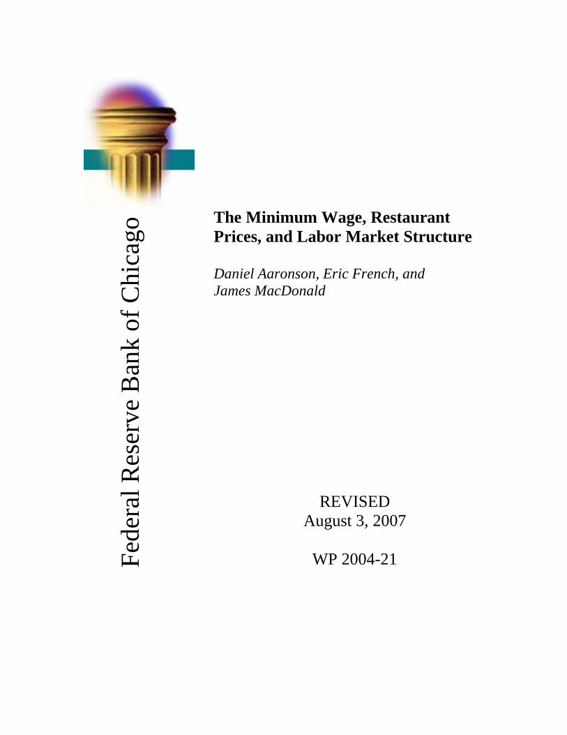
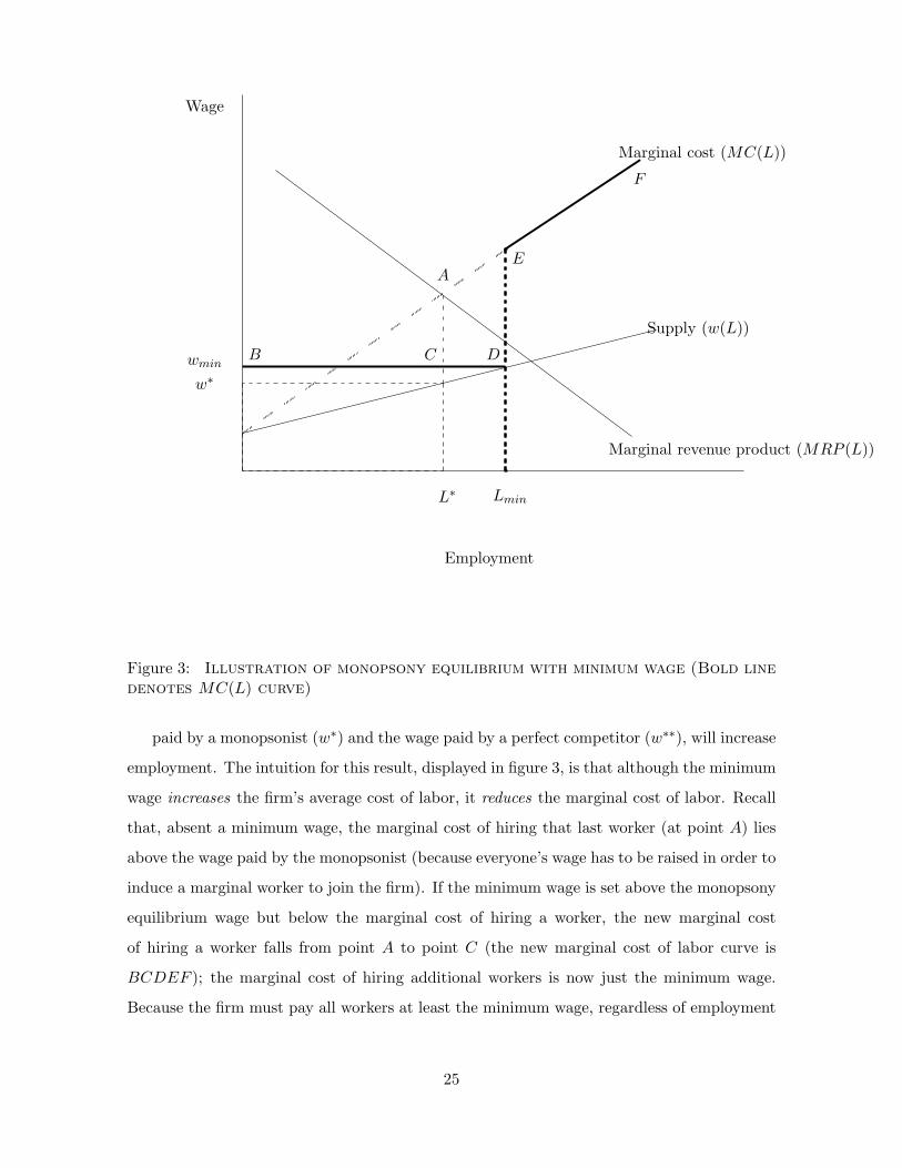
As a final alternative, we estimated logit models that explore the relationship between

minimum wage changes and the probability of a price increase or decrease by outlet type.

These regressions use a very similar specification to equation (1), but substitute ∆ ln pijkt

with an indicator of whether there is a price increase (pijkt > 0) in one specification and a

price decrease (pijkt < 0) in another.30 The first four columns of table 3 report a specification

that includes the lag, contemporaneous, and lead minimum wage change measure, along with

the controls described in the table. We find that the likelihood of a price increase in LS outlets

jumps from 12 to 28 percent if a 10 percent increase in the minimum wage is introduced in a

28There is some debate on the extent to which minimum wage increases impact workers paid above theminimum. See Card and Krueger (1995), Abowd et al (2000), and Lee (1999). We have experimented withusing those at or below the new minimum wage, as well as allowing for spillovers up to 20 percent above thenew minimum. This has little impact on the results.

29For identification, we must drop the PPI controls in this specification.30The main deviation from equation (1) is that we include a dummy for prices ending in 99 cents, to account

for the extra stickiness apparent at such price points. See MacDonald and Aaronson (2006) or Kashyap (1995)for further discussion. In the version reported here, we also include three lags in changes in item prices, anindicator of whether any sampled price was changed by the outlet in the previous period, and indicators formeal type. Inferences are not contigent on the inclusion of these additional covariates.

16

period with otherwise stable prices. The probability of a price increase in FS establishments

increases from 10 to 13 percent following a similar sized minimum wage change. However,

a 10 percent increase in the minimum wage has no statistically significant impact on the

probability of a price decline in either type of establishment. The final two columns show

that MSAs with a lower 20th percentile wage are much more likely to see price increases

in both LS and FS establishments after a minimum wage increase. There is no such effect

among price declines (not shown).

17

Establishment type Limited service Full service Limited service Full service Limited Service Full ServicePrice change Increase Increase Decrease Decrease Increase IncreaseColumn 1 2 3 4 5 6

∆ lnwmin,it−1 0.010 0.019 -0.007 0.004(0.014) (0.011) (0.022) (0.018)

∆ lnwmin,it 0.104 0.027 -0.020 0.008 0.253 0.233(0.012) (0.011) (0.021) (0.022) (0.095) (0.092)

∆ lnwmin,it+1 0.017 0.010 -0.029 0.014(0.015) (0.012) (0.029) (0.021)

wage20 ∗ ∆ lnwmin,it -0.024 -0.032(0.015) (0.014)

Constant -1.974 -2.150 -3.732 -4.403 -1.842 -2.485(0.074) (0.063) (0.137) (0.136) (0.444) (0.381)

Base Probability of price change 0.122 0.104 0.023 0.012 0.137 0.077After 10% minimum wage increase 0.282 0.132 0.019 0.013at wage20=$5 0.349 0.189at wage20=$7 0.241 0.121at wage20=$9 0.158 0.076

Coefficients and standard errors are derived from a logit model.See text for detail. Controls not shown in table include whether the price ended in 99 cents,three lags in ln pijkt, an indicator for whether any sampled price item was changed in the previous period,and mealtype (breakfast, lunch, or dinner).

Table 3: The Probability of a Price Increase or Decrease in Response to a 10 Percent Minimum Wage Increase

18

3.3 City-level Price Responses

The micro data suggest that prices move higher in response to minimum wage changes

that occurred between 1995 and 1997. In this section, we show that the results are robust to

looking at a longer earlier period. Here, we use the publicly available city-level price indices

of the CPI between 1979 and 1995 to test whether cities with higher fractions of restaurant

workers impacted by the minimum wage laws are more likely to change their food prices.

Hence, identification is based on the intensity of minimum wage worker usage. Our results

are based on a slightly modified form of equation (1):

∆ ln pit

∆ lnwmin,it= γprob(wit = wmin,it) + β′xit + uit (2)

where i denotes city and the coefficient γ = E[ ∆ ln pit

∆ ln wmin,it|wit = wmin,it, xit] is the price

response to increases in the minimum wage. If producers have a constant returns to scale

production function, competitive theory implies that 100 percent of the higher labor costs

are passed on to the consumer in the form of higher prices. As we pointed out earlier, 100%

pass through implies that the percent increase in product price equals the percent increase

in the minimum wage multiplied by labor’s share. Therefore, γ should equal labor’s share

under perfect competition.

Figure 1 maps each city’s price response to a minimum wage hike against the share of

minimum wage workers in the city. Each observation, of which there are 82, represents a

city around the time of a minimum wage change. The data cover 4 federal minimum wage

hikes - in 1980, 1981, 1990, and 1991 – and a small number of state increases between 1979

and 1995.31 The horizontal axis plots prob(wit = wmin,it), the share of workers in a city’s

restaurant industry that are paid the minimum wage. This is computed from the outgoing

rotation files of the Current Population Survey (CPS). Because employees paid just above

the minimum wage are also affected by the law, we include anyone paid within 120 percent of

31The federal minimum wage increased from $2.90 to $3.10 per hour in January 1980, to $3.35 in January1981, to $3.80 in April 1990, and to $4.25 in April 1991. State increases tend not to occur in states representedby CPI survey cities. The 27 CPI cities are New York City, Philadelphia, Boston, Pittsburgh, Buffalo,Chicago, Detroit, St Louis, Cleveland, Minneapolis-St. Paul, Milwaukee, Cincinnati, Kansas City, DC, Dallas,Baltimore, Houston, Atlanta, Miami, Los Angeles, San Francisco, Seattle, San Diego, Portland, Honolulu,Anchorage, and Denver. After 1986, prices for 12 of these cities – Buffalo, Minneapolis-St. Paul, Milwaukee,Cincinnati, Kansas City, Atlanta, San Diego, and Seattle, Portland, Honolulu, Anchorage, and Denver – arereported semiannually. Therefore, we only include pre-1986 observations for these cities.

19

-0.6

-0.4

-0.2

0

0.2

0.4

0.6

0.8

1

1.2

0 0.1 0.2 0.3 0.4 0.5 0.6 0.7 0.8 0.9 1

Share of city restaurant workers that are within 20% of the old minimum wage during previous 9

months

Ch

an

ge

in

lo

g c

ity f

oo

d a

wa

y f

rom

ho

me

pri

ce

/ c

ha

ng

e in

lo

g

min

imu

m w

ag

e

Figure 1: City level price increases

20

the old minimum wage during the nine months prior to the minimum wage enactment date.

However, the results are not sensitive to picking reasonable thresholds other than 120 percent

or time frames other than nine months. The vertical axis displays ∆ ln pit

∆ ln wmin,it, the ratio of

the log change in city food away from home prices to the log change in the city’s minimum

wage. The price data is the CPI for food away from home. The price changes are measured

from two months before to two months after the minimum wage is enacted. ∆ ln pit

∆ ln wmin,itis

adjusted for year fixed effects to account for inflation and other secular changes in national

labor market conditions.

The most noteworthy aspect of figure 1 is the positive correlation between the two series.

The regression coefficient γ is 0.36 with a robust, city clustered-corrected standard error of

0.24.32 Not only is the sign of this coefficient consistent with competition but the magnitude

is as well. Assuming perfect competition in the labor market, the regression coefficient should

equal labor’s share. Recall from section 3, labor’s share is approximately 30 to 35 percent.

Note also the abundance of observations on ∆ ln pit

∆ ln wmin,itthat are positive. Of the 82 city-

year observations, 19 are negative, including only 2 of the largest 30 price responses, defined

as when | ∆ ln pit

∆ ln wmin,it| > 0.20. These two are interesting in that they come from the same city,

Denver, over consecutive years, 1980 and 1981. Unfortunately, we have little information as

to what was happening in Denver during this time but we can highlight it for being the main

example where city-level prices fall quickly in response to a minimum wage change.33

The most plausible alternative explanation for these price responses is that they are driven

by shocks to demand that happen to be correlated with changes to the minimum wage. We

tried two ways to test this possibility. First, we estimated equation 2 without year fixed effects

but included changes in the city CPI in the xit vector. The intercept from this specification

is not statistically different from zero, suggesting that prices do not rise after minimum wage

hikes in areas where the minimum wage does not bind. This finding is consistent with the

32Using the share of minimum wage workers within 110 percent of the old minimum, rather than 120 percent,the point estimate (and adjusted standard error) is 0.42 (0.24). A Huber biweight regression procedure impliesa point estimate of 0.28 (0.16) and 0.42 (0.15) using the 110 and 120 percent minimum wage share thresholds.Finally, out of concern that inflation, even over this short period, are driving our results, we tried two things.First, when we include city price deflators as controls on the right hand side, the point estimates are roughly0.50 with t-statistics of roughly 2 to 2.5. Alternatively, we look at price changes only over the two months afterthe minimum wage change. In this case, the point estimate is between 0.20 and 0.30, again with t-statisticsof roughly 2 to 2.5.

33Since Denver is one of the 12 cities surveyed semiannually starting in 1986, we do not include the 1990and 1991 Denver data points in the figure. However, they are both positive, albeit small: 0.19 for 1990 and0.09 for 1991.

21

view that demand shocks are not confounding our estimates because if they were, we would

expect that prices would rise in areas where the minimum wage does not bind.

As a second check, we searched for alternative measures of pit that vary by local demand

conditions, are available for our city panel, and, most importantly, are relatively unaffected

by low wage labor costs. By far, the two best candidates are housing and medical care.

Therefore, we reran the regression described above, but substituted food away from home

prices with these two indices. As expected, we find no evidence that minimum wage hikes

are associated with price hikes for housing and medical care.34

Finally, we can compare the estimates in table 2 to predicted pass-through under com-

petition and constant returns to scale technology using metro variation in restaurant wage

distributions from the outgoing rotation files of the CPS. Under competition, the relation-

ship between these predicted price responses and the share of restaurant workers impacted

by minimum wage laws should correspond to labor share.

To conduct this test, we define two groups of cities. High wage cities are those with an

average hourly wage among the top fifth of all metropolitan areas in 1997-98. Low wage cities

are those with average wages among the bottom fifth of all metropolitan areas in 1997-98.

Among high (low) wage cities, 34 (59) percent of all restaurant workers are paid within 120

percent of the minimum wage, our rough measure of the share of workers impacted by such

laws. Based on the estimates in column (4) of table 2, the average predicted price response

for low and high wage cities is 0.097 and 0.090, respectively.35 The relationship between these

variables (slope of the line connecting high and low wage cities) is .97−.90.59−.34 = 0.28, slightly

lower than, and statistically indistinguishable from, observed labor share in the restaurant

industry. Furthermore, we get a similar labor share prediction when we estimate equation

(2) using the store-level data.36

34For housing, γ (and its adjusted standard error) is -0.31 (0.33). For medical care, it is -0.06 (0.33).35The 20th percentile restaurant wage in the high wage cities is $5.25, compared to $4.82 in the low wage

cities.36To derive γ from the micro data, we use the regression results from column 4 of table 2, which gives the

relationship between ∆ ln pit

∆ ln wmin,itand the 20th percentile of city market wage. Next, we regress the share of

workers in a city’s restaurant industry that are paid the minimum wage, prob(wit = wmin,it), on the 20thpercentile of that city’s market wage. Using the 27 major CPI cities during 1995 to 1997, the point estimatefrom this latter regression is prob(wit = wmin,it) = 0.839− 0.068×wage20it + νit, where wage20it is the 20thpercentile of city i’s wage distribution at time t. From these two regression equations, we can solve γ = 0.24.Ideally we could precisely estimate equation (2) using the micro data. Unfortunately, as we note in footnote 25,the number of observations in the CPS for individual cities can be small. Consequently, prob(wit = wmin,it)cannot be precisely estimated. But wage20it can.

22

4 Theory

In this section, we show how our results contribute to the debate on the employment effects

of the minimum wage. Assorted models offer differing explanations for why the estimated

employment responses to minimum wage hikes are small. As we point out below, however,

most of these models imply that prices either do not change or fall in response to a minimum

wage hike. Therefore, our results provide evidence against models that have been used to

explain the small employment responses found in the minimum wage literature.

Throughout the discussion we assume that all firms are profit maximizers and thus set

the level of employment, L, at the point where the marginal cost of the last worker hired

MC(L) is equal to the extra revenue she produces (her marginal revenue product of labor,

or MRP (L)). Appendices A and B contain the formal details of the model.

4.1 The Competitive Model

We begin by briefly considering the textbook competitive model. If a minimum wage is

introduced (or increased) beyond the market-clearing wage in a competitive labor market,

the marginal cost of hiring a worker increases. In response, holding all else equal, firms will

move along their downward sloping marginal revenue product of labor curve until they reach

the point where MRP (L) is again equated to marginal cost. Higher MRP (L) can only be

obtained by reducing the workforce. Why? One important reason is that fewer workers imply

less output. Even if an additional worker produced the same amount as the previous worker,

reduced output increases output prices, marginal revenue, and thus the marginal revenue

product of labor. Therefore, minimum wage hikes cause prices to rise and employment to fall

in a competitive labor market environment.

4.2 The Textbook Monopsony Model

However, under monopsony, increasing the minimum wage can cause employment to rise.

The fundamental reason is tied to the link between the wage, the marginal cost of labor,

and the product price. In this section we describe the textbook model of monopsony, where

firms are monopolists in the product market and monopsonists in the labor market. In

Section 4.3 we show that the key results hold under the more realistic scenario of monopolistic

competition in the product market and monopsonistic competition in the labor market.

23

Wage

L∗

w∗∗

L∗∗

Marginal cost (MC(L))

Supply (w(L))

w∗

A

Marginal revenue product (MRP (L))

Employment

Figure 2: Illustration of monopsony equilibrium

Unlike the competitive firm, which pays the prevailing market wage regardless of how

much labor it demands, if the monopsonist wants to expand its labor force, it has to raise

the wage of its current workers as well.37 Therefore, the marginal cost of hiring a worker

is greater than the new worker’s wage. Figure 2 shows the wage the firm would have to

pay in order to attract an additional worker, w(L), and the marginal cost of hiring that

worker MC(L). When the monopsonist maximizes profits by setting marginal costs equal

to marginal product, shown at point A, total market employment, L∗, is lower than the

“competitive case” (L∗∗) where employment is set based on the prevailing market wage w∗∗.

A properly placed minimum wage, set somewhere between the wage

37This is true if the monopsonist cannot perfectly discriminate between workers with high reservation wagesand low reservation wages.

24

Wage

L∗

wmin

Lmin

Marginal cost (MC(L))

Supply (w(L))

w∗

Marginal revenue product (MRP (L))

Employment

A

B C D

E

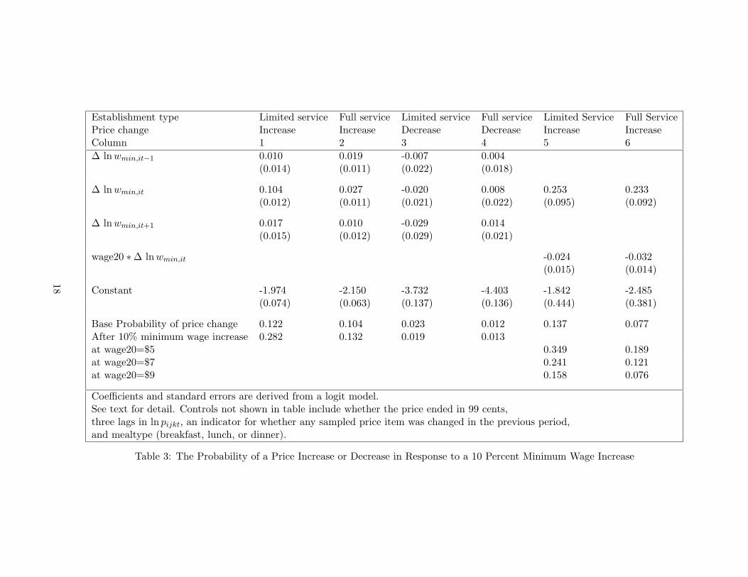
F

Figure 3: Illustration of monopsony equilibrium with minimum wage (Bold linedenotes MC(L) curve)

paid by a monopsonist (w∗) and the wage paid by a perfect competitor (w∗∗), will increase

employment. The intuition for this result, displayed in figure 3, is that although the minimum

wage increases the firm’s average cost of labor, it reduces the marginal cost of labor. Recall

that, absent a minimum wage, the marginal cost of hiring that last worker (at point A) lies

above the wage paid by the monopsonist (because everyone’s wage has to be raised in order to

induce a marginal worker to join the firm). If the minimum wage is set above the monopsony

equilibrium wage but below the marginal cost of hiring a worker, the new marginal cost

of hiring a worker falls from point A to point C (the new marginal cost of labor curve is

BCDEF ); the marginal cost of hiring additional workers is now just the minimum wage.

Because the firm must pay all workers at least the minimum wage, regardless of employment

25

level, the firm does not have to increase the pay of its existing workforce to attract more

employees (so long as employment is below Lmin). This reduction in the marginal cost of

hiring additional labor causes firms to expand output and employment in response to the

minimum wage increase.

Moreover, employment and prices are negatively related because the fall in the marginal

cost of labor causes the marginal cost of producing an extra unit to fall. Consequently, the

product price falls as well.

It is important to note that if firms are monopsonists in the labor market but the mini-

mum wage is set sufficiently high (above w∗∗ in Figure 2), employment is determined by the

intersection of the minimum wage and the marginal product of revenue curve. In this case, an

increase in the minimum wage increases prices and reduces employment, just like in a com-

petitive labor market. Thus our empirical results cannot necessarily disprove the existence of

monopsony labor markets in cases where the minimum wage is set high (above competitive

market-clearing levels). However, we believe our empirical results should temper enthusiasm

for monopsony power being the explanation for the negligible employment responses found

in the literature.

4.3 Price and Employment Responses when there is Monopsonistic Com-

petition in the Labor Market and Monopolistic Competition in the

Product Market

The results in the previous section were based on a very stylized model. In this section,

we show that those results are quite general under weak assumptions about technology,

the product market, and the labor market. Specifically, the results hold when firms have

a production function with substitutability between labor and other inputs, monopolistic

competition in the product market, and monopsonistic competition in the labor market.

Several researchers have argued that monopsonistic competition in the labor market is

the relevant case (Bhashkar and To (1999), Dickens et al. (1999)). That is, workers are

not indifferent between employers, even if all employers pay the same wage. One plausible

explanation is geography. Employers are located in different places and transportation costs

are large relative to earnings of minimum wage workers. Thus a worker is willing to take

a low paying job in order to be relatively near home. Alternatively, teenagers may want to

26

work at the same restaurant as their friends. More generally, certain aspects of one employer

may be disagreeable to some workers but not others.

In order to simplify the problem, we make six assumptions beyond the usual axioms of

firm behavior:

Assumption 1 There is a fixed number N of firms.

Assumption 2 All firms have an identical production function, Qn = Q(Kn, Ln) where

Qn, Kn, Ln are output, an aggregator of non-labor input (that includes capital), and labor at

the nth firm.

Assumption 3 The production function is increasing in all inputs, concave, continuous and

twice differentiable.

Assumption 4 K and L are complementary inputs in the production function (Q12 > 0).

Assumption 5 The utility function of the representative consumer is U =

(

(1 − α)Q1−η0 +

αQ1−η

) 1

1−η

, where Q0 is the numeraire good, α is close to zero, Q ≡(

∑Nn=1 Q

1−ηZn

) 1

1−ηZ ,

and Qn denotes output at the nth restaurant. Concavity implies η > 0 and ηZ ∈ [0, 1).

Assumption 6 The firm is a price taker in the capital market and purchases Kn at price

r. However, the firm is potentially a monopsonist in the labor market. The quantity of labor

supplied to the firm is LSn = L(wn, w−n), where w−n is the average wage paid by all other

firms, dL(wn,w−n)dwn

∣

∣

∣

∣

w−n=wmin

> 0, and dL(wn,w−n)dwn

∣

∣

∣

∣

w−n=wn

> 0.

Under these assumptions, firms sell their products at a price p(Q) and choose inputs to

maximize profits π :

πn(Kn, Ln) = p(Qn)Qn − wnLn − rKn. (3)

These assumptions are standard, although a few require some elaboration. Assumption

5 gives rise to monopolistic competition in the product market. Markets are perfectly com-

petitive if ηZ = 0 and firms operate as monopolists if ηZ = η. Assumption 6 states that the

quantity of labor supplied to the firm need not be perfectly elastic and, therefore, firms face a

27

monopsonistically competitive labor market. Consequently, firms face a weakly upward slop-

ing inverse labor supply curve, w(Ln), where dw(Ln,w−n)dLn

≥ 0. However, because the minimum

wage potentially binds, the offered wage is wn = maxw(Ln, w−n), wmin.38

Firms may be price takers in the labor market because the labor supply curve that the

firm faces is perfectly elastic or the minimum wage is sufficiently high that it destroys the

firm’s monopsony power. Either way, if firms are price takers in the labor market, Theorem

1 holds.

Theorem 1 Given the assumptions above, and if firms are price takers in the labor market,

the industry level demand curve for labor slopes down.

Proof: see Appendix A. Theorem 1 is more general than the discussion in Section 4.1.

There, it is presumed that firms make employment decisions given a fixed MRP (L) curve,

an assumption that is appropriate for monopolists. But, under monopolistic competition,

minimum wage changes potentially shift the MRP (L) curve by altering the decision of other

firms, and thus influencing aggregate prices. Theorem 1 also differs from the Weak Axiom

of Profit Maximization, which assumes perfect competition in both the product and factor

markets.39

Section 4.2 discusses why employment can rise under monopsony. Given assumption 6,

this is true under monopolistic competition as well. Together with Theorem 1, this shows that

minimum wage hikes cause employment to fall under competition and rise under monopsony.

The next theorem shows that we can use prices to infer the importance of monopsony

power in the labor market.

Theorem 2 Given an increase in a binding minimum wage, prices rise under perfect com-

petition and, so long as wmin < w∗∗, prices fall under monopsony.

38The assumption of capital and labor being complementary inputs (i.e. Q12 > 0) rules out situations wherethe profit maximizing choice would be to switch from a capital intensive, high output technology to a laborintensive, low output technology. An example of this is a firm that is capital efficient only up to a certain size.After this size, capital cannot be efficiently used. For example, suppose p = 1, r = 1, Q = K.5L.5 if L < 10 andQ = L.5 if L ≥ 10. Increasing L from 9 to 10 would reduce output but depending on the cost of labor, couldincrease profits. However, this rather extreme counter-example appears to go against the empirical evidence.For example, it is difficult to reject the hypothesis that production functions are constant returns to scale,and constant returns production functions implicitly assume Q12 > 0.

39See Varian (1984) and Kennan (1998) for proofs of Theorem 1 under competition and monopoly, respec-tively. We have also proved the theorems in this section for the case where firms are Cournot competitors inthe output market. Proofs are available from the authors.

28

Proof: see Appendix A. The intuition for Theorem 2 was discussed in Section 4.2.

Finally, there is the quantitative importance of price pass through when there is monop-

olistic competition in the product market. Theorem 3 shows that if the production function

is constant elasticity of substitution, then firms still push 100% of the higher labor costs onto

consumers in the form of higher prices.

Theorem 3 If Q(., .) is a constant elasticity of substitution aggregator, and if firms are price

takers in the labor market, then d ln pd ln wmin

= minimum wage labor’s share.

Proof: see Aaronson and French (2007). The intuition for this result is straightforward.

Given the assumptions above, firms have a constant marginal cost and thus have a horizontal

supply curve. Thus, in a perfectly competitive market, all higher labor costs will be pushed

onto consumers in the form of higher prices. In the case of monopolistic competition in the

product market, there is a constant mark-up over marginal cost. Thus the supply curve is

still horizontal and all labor costs are pushed onto consumers in the form of higher prices.

Furthermore, Aaronson and French give predicted price and employment responses under

monopsonistic competition. They show that if the employment response is large and positive,

then the price response will be large and negative. For example, if the employment elasticity

is +0.2, which is possible under monopsony, then the price response will be -0.05. These price

responses vary notably from what is reported in Table 2.

The only assumption that we view as not innocuous is the first. Although the size of a

business is allowed to change in response to a higher minimum wage, firm exit or entry is

precluded. We think this is a reasonable assumption given the existing, albeit rather meager,

empirical evidence.40 Moreover, in this paper, we are interested in a short-term response that

likely severely limits entry and exit decisions.

The main reason for assuming no exit is that under monopsony, minimum wage hikes in-

crease employment per restaurant, but likely reduce the total number of restaurants. There-

40Card and Krueger (1995) and Machin and Wilson (2004) find no effect in the U.S. and U.K., respectively.We have done some analysis of restaurant entry and exit using the Census’ Longitudinal Business Database.Consistent with the literature, our preliminary findings suggest negligible entry and exit effects in the yearfollowing a minimum wage change. These results stand in contrast to those of Campbell and Lapham (2004),who find a significant amount of retail net entry along the U.S.-Canada border within a year of exchange ratemovements. We suspect these different results reflect the importance of exchange rates relative to minimumwage levels in terms of firm costs.

29

fore, the industry level employment response is ambiguous. In this sense, we view the as-

sumption of no exit as supporting the monopsony argument.41

4.4 Efficiency Wage Models

Efficiency wage models (where increased wages increase effort or reduce turnover costs),

often give monopsony like predictions. Manning (1995), Rebitzer and Taylor (1995), and

Deltas (1999) all present models where increases in the minimum wage can increase employ-

ment. None of these models allows for capital-labor substitutability, and only Deltas (1999)

allows for endogenous prices. Below we present an efficiency wage model with endogenous

prices and capital-labor substitutability.

We follow Solow (1979), who argues that the wage affects morale and effort amongst

other things, and let the wage enter the production function directly. If an increase in the

wage causes increased effort, more meals can be produced with the same amount of labor and

capital. Therefore, it is not necessarily more costly to produce meals when the minimum wage

increases. This can attenuate the disemployment effects of the minimum wage. However, if

employment does not fall (and other factors do not fall either) and productivity rises, total

output will rise and product prices will fall.

Let the production function be:

Q = Q(K, L, w) =(

(1 − α)Kρ + α(Lwθ)ρ) 1

ρ , (4)

where σ ≡ 11−ρ

is the partial elasticity of substitution between K and Lwθ in the production

of Q, and Lwθ is “effective labor”. The parameter 0 ≤ θ < 1 may be greater than 0

because increases in the wage increase effort, which could happen for a variety of reasons.

Furthermore, assume that Assumptions 1 to 5 in Section 4.3 hold. Then the price and

41Nevertheless, we also understand that, given our assumed market structure, entry and exit can changethe market price for a given industry output. This is potentially important because Bashkar and To (1999)argue that an increase in the minimum wage could reduce the number of firms in the market but increaseemployment per restaurant, causing total employment to potentially increase. Because the number of firmsdecrease, market power of survivors increase. Consequently, both prices and output may increase. However,given the small observed exit rates in response to minimum wage hikes, we doubt that these effects would belarge enough to overturn the basic presumption that market output and price move in opposite directions.

30

employment responses are:

d ln p

d lnw= s(1 − θ) (5)

d lnL

d lnw= −(1 − θ)

(

(1 − s)σ − sη)

− θ (6)

where s is the share of total costs going to labor. When θ = 0, equations (5) and (6) give

the textbook response to the minimum wage. However, when θ > 0 (and all else is equal),

a one percent increase in the wage increases effective labor θ percent, causing the marginal

cost of effective labor to only rise 1 − θ percent. This has implications for both prices and

employment responses. The price response is attenuated, rising by s(1−θ) percent, a fraction

(1 − θ) less than without endogenous work effort. The employment response is also muted

by (1 − θ) due to an increase in the marginal cost of labor. However, the same amount of

effective labor and output can be produced with fewer bodies, lessening the need for labor

(the −θ term at the end of equation (6)).

Regardless, while a smaller employment response relative to the case without endogenous

work effort is possible, the model clearly predicts a smaller price response as well. However,

our estimates indicate large price responses to the minimum wage. Thus, our price results

provide evidence against the hypothesis that endogenous work effort is responsible for the

small observed employment responses to minimum wage hikes.

4.5 Other Models of the Employment Effects of the Minimum Wage

We have argued that the price responses to minimum wage hikes are useful for distin-

guishing between competition and monopsony in the labor market. Likewise, our estimated

price responses help shed light on other explanations of the small employment response found

in the minimum wage literature.

Some researchers (e.g. Kennan 1995, MaCurdy and OBrien-Strain 2000) suggest higher

income resulting from a minimum wage increase causes low wage workers to buy more min-

imum wage products, attenuating the disemployment effect of the minimum wage. For the

restaurant industry, Kennan refers to this possibility as the ”hungry teenager hypothesis.”

The price response reported in this paper is a key parameter for such a calculation. Aaronson

31

and French (2006) write down a model that allows for such demand-induced feedbacks and

show that increases in the minimum wage reduce real income for non-minimum wage workers

(because prices rise) but increase real income of minimum wage workers (because their wage

rises). They find that if minimum wage workers spend a large fraction of their income on fast

food, then the rise in incomes for fast food workers can at least partly offset the disemploy-

ment effect of the minimum wage. Using data from the Consumer Expenditure Survey and

US Department of Agriculture’s Continuing Survey of Food Intake by Individuals, they find

that minimum wage workers spend between 20 and 100% more of their income on fast food

as those who are not minimum wage workers.42 Given these estimates (and other calibrated

parameters) the increased income going to minimum wage workers can offset between 25 and

40% of the output loss, and 10 to 30% of the employment loss of a model that does not

account for the increased income and increased expenditures of minimum wage workers.

Our price responses are less consistent with the idea that that minimum wage laws merely

cause firms to reshuffle compensation packages from non-wage benefits to wages. For exam-

ple, fast food restaurants could stop giving workers free meals after minimum wage hikes.

Hashimoto (1982) and Neumark and Wascher (2001) argue that firms may reduce training

after minimum wage hikes. As a result, there is no increase in the cost of labor faced by firms.

However, if the minimum wage does not increase the cost of labor, it is unclear why there

are price increases after minimum wage changes. Although shifting compensation packages

from non-wage to wage benefits may occur, our results indicate that firms still bear a sizeable

fraction of the cost of minimum wage hikes. In this sense, our findings are consistent with

Card and Krueger (1995), who also find very little substitution between wage and non-wage

benefits after minimum wage hikes and also find no evidence of minimum wage hikes on

training.

Finally, our analysis has not considered search models (e.g. Burdett and Mortensen

1998), which also give monopsony implications for employment. A full analysis of the variety

of search models is well beyond the scope of this paper, especially since most of them would

need to be modified to account for endogenous product prices and capital labor substituabil-

ity. However, it seems likely that employment and prices would move in opposite directions

in most standard applications of search. For example, given that the Burdett and Mortensen

42MaCurdy and OBrien-Strain (2000) also find that low income individuals spend a greater fraction of theirbudget on products produced by minimum wage workers.

32

production technology is linear in labor (i.e. no substitution among inputs), increases in

employment increase output and should presumably reduce the product price were it endo-

genized. It is also worth noting that most estimated search models, including Van den Berg

and Ridder (1998), Flinn (2006), Ahn and Arcidiacono (2003), find some disemployment in

response to a minimum wage increase.

Arguably, our empirical results themselves - that marginal cost shocks are passed onto

consumers through higher output prices - may be consistent with small disemployment effects.

If restaurants face factors that limit their ability to raise prices, say because it is costly to

switch prices, or because the price elasticity of demand for food away from home is infinitely

elastic, the predicted disemployment effects of a minimum wage increase would be larger

than if these factors did not hinder price behavior. If firms cannot pass cost increases onto

consumers, then profits will be squeezed and firms may sharply cut their workforce. Given

that we find rather large price increases in response to minimum wage hikes, firms seem to

be able to push costs onto consumers, and are not having their profits greatly reduced.

Instead, we interpret our results to be consistent with the moderate disemployment effects

reported in Aaronson and French (2007). They calibrate a structural model of labor demand

that incorporates the price responses found here to show that a 10 percent increase in the

minimum wage reduces restaurant employment by 2 to 3 percent, a short run response that

is within the range of estimates found in the literature. Moreover, the total (low plus high

skill) restaurant employment response may be as small as 1 percent.

5 Conclusion

Much work has looked at the employment implications of raising the minimum wage,

with a range of estimates reported in the literature. We offer new empirical evidence using

output prices both at the store-level and aggregated to the city-level. In both cases, prices

unambiguously increase in response to a minimum wage change. Furthermore, the results are

similar across three sources of variation in the data: cross-state differences in the size of the

minimum wage change, cross-restaurant type differences in the tendency to pay at or near

the minimum wage, and cross-metro differences in the fraction of workers paid at or near

the minimum wage. There is no evidence that prices fall in response to a minimum wage

increase.

33

We interpret these findings within a simple yet quite general model of employment deter-

mination that shows that monopsony and perfect competition have opposite implications for

not only employment but output prices as well, so long as the minimum wage is not set too

high. In particular, under monopsony, an increase in a binding minimum wage causes em-

ployment to rise and output prices to fall. Under competition, employment falls and output

prices rise. Therefore, our price results appear to provide evidence against the hypothesis that

monopsony power is important for understanding the small observed employment response

to minimum wage changes. Indeed, our estimated price responses provide evidence against

other explanations of the small employment response, including the potential substitution of

nonwage for wage compensation and the importance of endogenous work effort. Rather, we

interpret our price results to be fairly consistent with the textbook model of labor demand.

34

References

[1] Aaronson, Daniel “Price Pass-Through and the Minimum Wage,” Review of Eco-

nomics and Statistics, February 2001, 83(1), 158-169.

[2] Aaronson, Daniel and Eric French “Product Market Evidence on the Employment

Effects of the Minimum Wage,” Journal of Labor Economics, January 2007, 25(1), 167-

200.

[3] Aaronson, Daniel and Eric French “Can Income Effects Explain the Small Observed

Disemployment Reponse to Minimum Wage Changes ,” working paper, Federal Reserve

Bank of Chicago, 2006.

[4] Abowd, John, Francis Kramarz, David Margolis, and Thomas Philippon,

“The Tale of Two Countries: Minimum Wages and Employment in France and the

United States, working paper, INSEE-CREST, 2000.

[5] Ahn, Tom and Peter Arcidiacono “Minimum Wages and Positive Employment

Effects in General Equilibrium,” working paper, Duke University, 2003.

[6] Ashenfelter, Orley, and Stepan Jurajda, “Cross-country Comparisons of Wage

Rates: The Big Mac Index,” working paper, Princeton University, 2001.

[7] Bhaskar, V. and Ted To, “Minimum Wages for Ronald McDonald Monopsonies: A

Theory of Monopsonistic Competition,” Economic Journal, April 1999, 109(455), 190-

203.

[8] Bils, Mark and Peter Klenow, “Some Evidence on the Importance of Sticky Prices,”

Journal of Political Economy, October 2004, 112(5), 947-985.

[9] Boal, William and Michael Ransom, “Monopsony in the Labor Market,” Journal

of Economic Literature, March 1997, 35(1), 86-112.

[10] Brown, Charles, “Minimum Wages, Employment, and the Distribution of Income,”

in Ashenfelter and Card, eds. Handbook of Labor Economics, Vol 3B, 1999, Amsterdam:

North-Holland, 2101-2163.

35

[11] Brown, Charles, Curtis Gilroy, and Andrew Kohen, “The Effect of the Minimum

Wage on Employment and Unemployment,” Journal of Economic Literature, June 1982,

20(2), 487-528.

[12] Burdett, Kenneth, and Dale Mortensen, “Wage Differentials, Employer Size, and

Unemployment,” International Economic Review, May 1998, 39(2), 257-273.

[13] Burkhauser, Richard, Kenneth Couch, and David Wittenburg, “A Reassess-

ment of the New Economics of the Minimum Wage Literature with Monthly Data from

the Current Population Survey,” Journal of Labor Economics, October 2000, 18(4), 653-

680.

[14] Campbell, Jeffrey and Beverly Lapham “Real Exchange Rate Fluctuations and the

Dynamics of Retail Trade Industries on the U.S.-Canada Border,” American Economic

Review , September 2004, 94(4), 1194-1206.

[15] Card, David and Alan Krueger, Myth and Measurement: The New Economics of

the Minimum Wage, Princeton, NJ: Princeton University Press, 1995.

[16] Card, David and Alan Krueger, “Minimum Wages and Employment: A Case Study

of the Fast-Food Industry in New Jersey and Pennsylvania: Reply,” American Economic

Review, December 2000, 90(5), 1397-1420.

[17] Chevalier, Judith, Anil Kashyap, and Peter Rossi, “Why Don’t Prices Rise Dur-

ing Periods of Peak Demand? Evidence from Scanner Data,” American Economic Re-

view, March 2003, 93(1), 15-37.

[18] Converse, Muriel, Richard Coe, Mary Corcoran, Maureen Kallick, and James

Morgan, “The Minimum Wage: An Employer Survey,” in Report of the Minimum Wage

Commission, 1981, Washington DC: US Government Printing Office, 241-341.

[19] Deere, Donald, Kevin M. Murphy, and Finis Welch, “Employment and the 1990-

1991 Minimum-Wage Hike,” American Economic Review, May 1995, 85(2), 232-237.

[20] Deloitte and Touch, 2003 Restaurant Industry Operations Report, Washington, DC:

National Restaurant Association, 2003.

36

[21] Dickens, Richard, Stephen Machin, and Alan Manning, “The Effects of Min-

imum Wages on Employment: Theory and Evidence from Britain,” Journal of Labor

Economics, January 1999, 17(1), 1-22.

[22] Dixit, A. and J. Stiglitz, “Monopolistic Competition and Optimum Product Diver-

sity,” American Economic Review, June 1977, 67(3), 297-308.

[23] Flinn, Christopher, “Minimum Wage Effects on Labor Market Outcomes under

Search, Bargaining, and Endogenous Contact Rates,” Econometrica, forthcoming, 2006.

[24] Fuchs, Victor, Alan Krueger, and James Poterba, “Economists’ Views about

Parameters, Values, and Policies: Survey Results in Labor and Public Economics,”

Journal of Economic Literature, September 1998, 36(3), 1387-1425.

[25] Hashimoto, Masanori, “Minimum Wage Effects on Training on the Job,” American

Economic Review , December 1982, 72(5), pp. 1070-1087.

[26] Kashyap, Anil, “Sticky Prices: New Evidence from Retail Catalogs,” Quarterly Jour-

nal of Economics, February 1995, 110(1), pp. 245-274.

[27] Katz, Lawrence and Alan Krueger, “The Effect of the Minimum Wage on the Fast

Food Industry,” Industrial and Labor Relations Review, October 1992, 46(1), 6-21.

[28] Kennan, John, “The Elusive Effects of Minimum Wages,” Journal of Economic Lit-

erature, December 1995, 33(4), 1950-1965.

[29] Kennan, John, “Minimum Wage Regulation,” in Newman, ed. The New Palgrave

Dictionary of Economics and the Law, 1998, New York: Norton.

[30] Kim, Taeil and Lowell Taylor, “The Employment Effect in Retail Trade of Cali-

fornia’s 1988 Minimum Wage Increase,” Journal of Business and Economic Statistics,

April 1995, 13(2), 175-182.

[31] Lee, David, “Wage Inequality in the United States During the 1980s: Rising Dispersion

or Falling Minimum Wage?,” Quarterly Journal of Economics, August 1999, 114(3), 977-

1023.

[32] Machin, Stephen and Joan Wilson, “Minimum Wages in a Low-Wage Labour Mar-

ket: Care Homes in the UK,” The Economic Journal, March 2004, 114(494), C102-C109.

37

[33] MacDonald, James and Daniel Aaronson, “How Firms Construct Price Changes:

Evidence from Restaurant Responses to Increased Minimum Wages,” American Journal

of Agricultural Economics, May 2006, 88(2), 292-307.

[34] MaCurdy, Thomas and Margaret OBrien-Strain, “Increasing the Minimum Wage:

California’s Winners and Losers,” working paper, Public Policy Institute of California,

2000.

[35] Manning, Alan, “How Do We Know That Real Wages Are Too High?,” Quarterly

Journal of Economics, November 1995, 110(4), 1111-1125.

[36] Manning, Alan, Monopsony in Motion: Imperfect Competition in Labor Markets,

Princeton, NJ: Princeton University Press, 2003.

[37] Neumark, David and William Wascher, “Reconciling the Evidence on Employment

Effects of Minimum Wages: A Review of Our Research Findings,” in Kosters, ed. The

Effects of Minimum Wages on Employment, 1996, Washington, DC: American Enterprise

Institute, 55-86.

[38] Neumark, David and William Wascher, “Minimum Wages and Employment: A

Case Study of the Fast-Food Industry in New Jersey and Pennsylvania: Comment,”

American Economic Review, December 2000, 90(5), 1362-1396.

[39] Neumark, David and William Wascher, “ Minimum Wages and Training Revis-

ited,” Journal of Labor Economics, July 2001, 19(3), 563-595.

[40] Rebitzer, James and Lowell Taylor, “The Consequences of Minimum Wage Laws:

Some New Theoretical Ideas,” Journal of Public Economics, February 1995, 56(2), 245-

255.

[41] Rubin, Alissa, “Popular Minimum Wage Hike Gets Solid Senate Approval,” Congres-

sional Quarterly, July 13, 1996, 1964-1965.

[42] Solow, Robert, “Another Possible Source of Wage Stickiness,” Journal of Macroeco-

nomics, 1979, 1(1), 79-82.

[43] Stigler, George, “The Economics of Minimum Wage Legislation,” American Economic

Review, June 1946, 36(3), 358-365.

38

[44] van den Berg, Gerard and Geert Ridder, “An Empirical Equilibrium Search Model

of the Labor Market,” Econometrica, September 1998, 66(5), 1183-1223.

[45] Varian, Hal, “The Nonparametric Approach to Production Analysis,” Econometrica,

May 1984, 52(3), 579-597.

[46] Weisman, Jonathan, “Republican Defectors Help Propel Minimum Wage Bill to Pas-

sage,” Congressional Quarterly, May 25, 1996, 1461-1464.

39

Appendix A: Proofs

Proof of Theorm 1

Dixit and Stiglitz (1977) point out that two-stage budgeting techniques can be used

to analyze the consumer demand problem described in the text. In the second stage the

consumer solves:

maxQnN

n=1

(

N∑

n=1

Q1−ηZn

) 1

1−ηZ (7)

subject to

N∑

n=1

pnQn = X, (8)

where X is total expenditure on Q. The consumer’s first order condition for utility maxi-

mization yields

pn = λ−1

(

Qn

Q

)−ηZ

(9)

where λ is the Lagrange multiplier on the budget constraint for expenditure on Q, i.e., it is

the multiplier on the first stage constraint. If N is sufficiently large, then Qn is small relative

to Q and thus the firm does not take into account the effect of Qn on Q when assessing the

effect of Qn on pn.

Inserting equation (9) into equation (3) yields

π(Kn, Ln) = ΩQ1−ηZn − wnLn − rKn (10)

where Ω = λ−1QηZ . The first order condition for maximization of the profit function (10)

with respect to Kn yields

Ω(1 − ηZ)Q−ηZn Qn,1 = r (11)

where ∂Qn

∂Kn≡ Qn,1. If the firm is a price taker in the labor market, then employment is

40

determined by maximization of equation (10) with respect to Ln, which yields

Ω(1 − ηZ)Q−ηZn Qn,2 = w. (12)

where ∂Qn

∂Ln≡ Qn,2. First, we discuss the case where the firm is a price taker in the labor

market. Given the assumptions above, all firms are of equal size, so Q = N1

1−ηZ Qn. Because

of this, equation (9) shows that

d lnλ

d lnw= −

d ln p

d lnw, (13)

where the price index associated with Q is p ≡(

∑Nn=1 p

ηZ−1

ηZn

)

ηZηZ−1

. Using these definitions

and Assumption 5, one can show that d ln Qd ln p

= −η.

Because price changes are responses to supply shocks, price changes identify the demand

curve for the aggregate product, so d ln Qd ln p

= −η∗ for some η∗ ∈ (0, η], where η∗ = η if the

production technology is constant returns. Therefore, we may write

d ln p

d lnw=

d ln Qd ln w

d ln Qd ln p

= −1

η∗

(

d lnQn

d lnw

)

(14)

where we are assuming that d ln Nd ln w

= 0. Taking logs and differentiating equations (11) and

(12) with respect to lnw and inserting equations (13) and (14) yields

AndKn

dw+ Cn

dLn

dw= 0 (15)

BndKn

dw+ Dn

dLn

dw= 1 (16)

and differentiating equation (11) and (12) with respect to ln r and inserting equations anal-

ogous to (13) and (14) yields

AndKn

dr+ Cn

dLn

dr= 1 (17)

BndKn

dr+ Dn

dLn

dr= 0 (18)

41

where

An ≡ (−wQn,1

η∗Qn+

wQn,11

Qn,1) (19)

Bn ≡ (−wQn,1

η∗Qn+

wQn,12

Qn,2) (20)

Cn ≡ (−wQn,2

η∗Qn+

wQn,12

Qn,1) (21)

Dn ≡ (−wQn,1

η∗Qn+

wQn,22

Qn,2). (22)

In matrix form this can be rewritten as

An Cn

Bn Dn

dKn

drdKn

dw

dLn

drdLn

dw

=

1 0

0 1

which can be rewritten as

dKn

drdKn

dw

dLn

drdLn

dw

=1

AnDn − BnCn

Dn −Cn

−Bn An

where solving for AnDn −BnCn shows that the term is positive if the production function is

concave.

Solving for dKn

dwand dLn

dwyields

dLn

dw=

An

AnDn − BnCn(23)

dKn

dw=

−Cn

AnDn − BnCn. (24)

The term An is negative. Therefore, the quantity of labor demanded falls when the price

rises. The market employment change is N times the firm level employment change.

42

We consider the monopsony case next. Because both the production and utility functions

are smooth, small changes in the minimum wage result in small changes in the MRP (Ln),

denoted in equation (12). Therefore, employment is determined by labor supply, not labor

demand. Figure 3 clarifies this point. Given the assumed upward sloping labor supply curve,

employment rises in response to an increase in the minimum wage.

QED.

Proof of Theorem 2

Consider the case of perfectly competitive labor markets first. Define p, Q and L as the

market price, output and employment. Because all firms produce the same amount, p = pn,

Q = NQn and L = NLn for all n. The price response to the wage change is

dp

dw=

dp

dQ

dQ

dw(25)

where a Taylor’s series expansion shows

dQ

dw= N

(

Qn,1dKn

dw+ Qn,2

dLn

dw

)

. (26)

Inserting equations (23) and (24) into equation (26) yields

dQ

dw= N

(

−Qn,1Cn + Qn,2An

AnDn − BnCn

)

. (27)

The numerator of this expression is negative and the denominator is positive if Qn,12 > 0.

Therefore, dQdw

< 0. Since dpdQ

< 0 by assumption, dpdw

> 0 under perfectly competitive labor

markets.

Now consider the monopsony case. Recall that under the monopsony case, labor is deter-

mined by labor supply, not labor demand. Therefore, we can take labor supply as exogenous.

Therefore, we may rewrite equation (25) as:

dp

dw=

dp

dQ

dQ

dw=

dp

dQ

(

dQ

dL

dL

dw

)

. (28)

Since by assumption, dpdQ

< 0 and dLdw

> 0, all that remains is to prove that dQdL

> 0 when dL

is taken as exogenous in order to prove that dpdw

< 0 under monopsony.

43

Taking the log of equation (11) and differentiating with respect to lnL yields

d lnΩ

d lnL+

d lnQn,1

d lnL= 0 (29)

Because d ln λd ln L

= − d ln pd ln L

and for reasons discussed in the proof of Theorem 1, equation (29)

may be rewritten as

d ln p

d lnL+

d lnQn,1

d lnL= 0 (30)

Using d ln pd ln L

=d ln Qd ln Ld ln Qd ln p

we may rewrite equation (30) as

−1

η∗

(

d lnQn

d lnL+

d lnN

d lnL

)

+d lnQn,1

d lnL= 0 (31)

for some η∗ ∈ (0, η], where d ln Nd ln L

= 0. Using the chain rule,

dQn

dL= Qn,1

dKn

dL+ Qn,2, (32)

dQn,1

dL= Qn,11

dKn

dL+ Qn,12. (33)

Inserting equations (32) and (33) into (31) yields

(

−L

η∗Qn

)(

Qn,1dKn

dL+ Qn,2

)

+

(

L

Qn,1

)(

Qn,11dKn

dL+ Qn,12

)

= 0 (34)

Solving for dKn

dLand inserting this into equation (32) yields

dQn

dL= Qn,1

(

1η∗Qn

Qn,2 −1

Qn,1Qn,12

− 1η∗Qn

Qn,1 + 1Qn,1

Qn,11

)

+ Qn,2 (35)

where the term in parentheses is dKn

dL. The denominator of this term is negative. The first

term in the numerator is positive but the second term is non-positive, making the sign of the

numerator term in parentheses ambiguous. However, dQn

dLis positive. To see this, note that

44

|(

−Qn,1

η∗Qn

)

| < |(

−Qn,1

η∗Qn+

Qn,11

Qn,1

)

|. Therefore, |

(

Qn,2η∗Qn

−Qn,1η∗Qn

)

| > |

(

Qn,2η∗Qn

−Qn,1η∗Qn

+Qn,11Qn,1

)

| and thus

dQn

dL> Qn,1

(

−

Qn,2

η∗Qn

Qn,1

η∗Qn

)

+ Qn,1

(

−Qn,12

Qn,1

−Qn,1

η∗Qn+

Qn,11

Qn,1

)

+ Qn,2 = Qn,1

(

−Qn,12

Qn,1

−Qn,1

η∗Qn+

Qn,11

Qn,1

)

(36)

which is greater than 0 if Qn,12 is greater than 0. Therefore, dQn

dL> 0 and thus dQ

dL> 0 and

dpdw

< 0 under monopsony. QED.

Appendix B: Price and Employment Responses in Models with Endogenous

Work Effort

In this appendix we assume that firms are price takers in all markets (so ηZ = 0), although

using the results in Aaronson and French (2004) it is straightforward to account for the case

where ηZ > 0. That paper provides a similar and more detailed derivation than the one

below, although they assume θ = 0.

Maximization of equation (3) with respect to K and L, and taking logs, yields:

σ(ln r − ln p) = σ ln(1 − α) +(

lnQ − lnK)

, (37)

σ(lnw − ln p) = σ lnα +(

lnQ − lnL)

+ σρθ lnw. (38)

Assume that product prices potentially change in response to a change in the minimum wage,

but the price of capital does not. Differentiating equations (37) and (38) with respect to lnw,

and using results in Aaronson and French (2007), yields:

−σ(1

η

d lnQ

d lnw

)

= −d lnQ

d lnw+

d lnK

d lnw, (39)

−d lnL

d lnw= −

d lnQ

d lnw

(

1 −σ

η

)

+ (1 − σ)θ + σ, (40)

where η is the elasticity of demand for the product (in absolute value), as in the text. Fur-

thermore, differentiating the production function with respect to the wage yields:

dQ

dw=

∂Q

∂K

dK

dw+

∂Q

∂L

dL

dw+

∂Q

∂w. (41)

Solving for ∂Q∂w

as a function of ∂Q∂L

, noting that ∂Q∂L

= wp, ∂Q

∂K= r

p, and denoting s = wL

pQas

45

labor’s share, some algebra shows that equation (41) can be rewritten as:

d lnQ

d lnw= (1 − s)

d lnK

d lnw+ s

d lnL

d lnw+ sθ (42)

Using equations (39), (40), and (42), we can solve for the unknowns:

d lnQ

d lnw= −ηs(1 − θ), (43)

d lnK

d lnw= s(1 − θ)(σ − η), (44)

d lnL

d lnw= −(1 − θ)

(

(1 − s)σ − sη)

− θ. (45)

The price response will be

d ln p

d lnw= s(1 − θ). (46)

46

Working Paper Series

A series of research studies on regional economic issues relating to the Seventh Federal Reserve District, and on financial and economic topics.

Does Bank Concentration Lead to Concentration in Industrial Sectors? WP-01-01 Nicola Cetorelli On the Fiscal Implications of Twin Crises WP-01-02 Craig Burnside, Martin Eichenbaum and Sergio Rebelo Sub-Debt Yield Spreads as Bank Risk Measures WP-01-03 Douglas D. Evanoff and Larry D. Wall Productivity Growth in the 1990s: Technology, Utilization, or Adjustment? WP-01-04 Susanto Basu, John G. Fernald and Matthew D. Shapiro Do Regulators Search for the Quiet Life? The Relationship Between Regulators and The Regulated in Banking WP-01-05 Richard J. Rosen Learning-by-Doing, Scale Efficiencies, and Financial Performance at Internet-Only Banks WP-01-06 Robert DeYoung The Role of Real Wages, Productivity, and Fiscal Policy in Germany’s Great Depression 1928-37 WP-01-07 Jonas D. M. Fisher and Andreas Hornstein Nominal Rigidities and the Dynamic Effects of a Shock to Monetary Policy WP-01-08 Lawrence J. Christiano, Martin Eichenbaum and Charles L. Evans Outsourcing Business Service and the Scope of Local Markets WP-01-09 Yukako Ono The Effect of Market Size Structure on Competition: The Case of Small Business Lending WP-01-10 Allen N. Berger, Richard J. Rosen and Gregory F. Udell Deregulation, the Internet, and the Competitive Viability of Large Banks WP-01-11 and Community Banks Robert DeYoung and William C. Hunter Price Ceilings as Focal Points for Tacit Collusion: Evidence from Credit Cards WP-01-12 Christopher R. Knittel and Victor Stango Gaps and Triangles WP-01-13 Bernardino Adão, Isabel Correia and Pedro Teles A Real Explanation for Heterogeneous Investment Dynamics WP-01-14 Jonas D.M. Fisher Recovering Risk Aversion from Options WP-01-15 Robert R. Bliss and Nikolaos Panigirtzoglou Economic Determinants of the Nominal Treasury Yield Curve WP-01-16 Charles L. Evans and David Marshall

1

Working Paper Series (continued) Price Level Uniformity in a Random Matching Model with Perfectly Patient Traders WP-01-17 Edward J. Green and Ruilin Zhou Earnings Mobility in the US: A New Look at Intergenerational Inequality WP-01-18 Bhashkar Mazumder The Effects of Health Insurance and Self-Insurance on Retirement Behavior WP-01-19 Eric French and John Bailey Jones The Effect of Part-Time Work on Wages: Evidence from the Social Security Rules WP-01-20 Daniel Aaronson and Eric French Antidumping Policy Under Imperfect Competition WP-01-21 Meredith A. Crowley Is the United States an Optimum Currency Area? An Empirical Analysis of Regional Business Cycles WP-01-22 Michael A. Kouparitsas A Note on the Estimation of Linear Regression Models with Heteroskedastic Measurement Errors WP-01-23 Daniel G. Sullivan The Mis-Measurement of Permanent Earnings: New Evidence from Social WP-01-24 Security Earnings Data Bhashkar Mazumder Pricing IPOs of Mutual Thrift Conversions: The Joint Effect of Regulation and Market Discipline WP-01-25 Elijah Brewer III, Douglas D. Evanoff and Jacky So Opportunity Cost and Prudentiality: An Analysis of Collateral Decisions in Bilateral and Multilateral Settings WP-01-26 Herbert L. Baer, Virginia G. France and James T. Moser Outsourcing Business Services and the Role of Central Administrative Offices WP-02-01 Yukako Ono Strategic Responses to Regulatory Threat in the Credit Card Market* WP-02-02 Victor Stango The Optimal Mix of Taxes on Money, Consumption and Income WP-02-03 Fiorella De Fiore and Pedro Teles Expectation Traps and Monetary Policy WP-02-04 Stefania Albanesi, V. V. Chari and Lawrence J. Christiano Monetary Policy in a Financial Crisis WP-02-05 Lawrence J. Christiano, Christopher Gust and Jorge Roldos Regulatory Incentives and Consolidation: The Case of Commercial Bank Mergers and the Community Reinvestment Act WP-02-06 Raphael Bostic, Hamid Mehran, Anna Paulson and Marc Saidenberg

2

Working Paper Series (continued) Technological Progress and the Geographic Expansion of the Banking Industry WP-02-07 Allen N. Berger and Robert DeYoung Choosing the Right Parents: Changes in the Intergenerational Transmission WP-02-08 of Inequality Between 1980 and the Early 1990s David I. Levine and Bhashkar Mazumder The Immediacy Implications of Exchange Organization WP-02-09 James T. Moser Maternal Employment and Overweight Children WP-02-10 Patricia M. Anderson, Kristin F. Butcher and Phillip B. Levine The Costs and Benefits of Moral Suasion: Evidence from the Rescue of WP-02-11 Long-Term Capital Management Craig Furfine On the Cyclical Behavior of Employment, Unemployment and Labor Force Participation WP-02-12 Marcelo Veracierto Do Safeguard Tariffs and Antidumping Duties Open or Close Technology Gaps? WP-02-13 Meredith A. Crowley Technology Shocks Matter WP-02-14 Jonas D. M. Fisher Money as a Mechanism in a Bewley Economy WP-02-15 Edward J. Green and Ruilin Zhou Optimal Fiscal and Monetary Policy: Equivalence Results WP-02-16 Isabel Correia, Juan Pablo Nicolini and Pedro Teles Real Exchange Rate Fluctuations and the Dynamics of Retail Trade Industries WP-02-17 on the U.S.-Canada Border Jeffrey R. Campbell and Beverly Lapham Bank Procyclicality, Credit Crunches, and Asymmetric Monetary Policy Effects: WP-02-18 A Unifying Model Robert R. Bliss and George G. Kaufman Location of Headquarter Growth During the 90s WP-02-19 Thomas H. Klier The Value of Banking Relationships During a Financial Crisis: WP-02-20 Evidence from Failures of Japanese Banks Elijah Brewer III, Hesna Genay, William Curt Hunter and George G. Kaufman On the Distribution and Dynamics of Health Costs WP-02-21 Eric French and John Bailey Jones The Effects of Progressive Taxation on Labor Supply when Hours and Wages are WP-02-22 Jointly Determined Daniel Aaronson and Eric French

3

Working Paper Series (continued) Inter-industry Contagion and the Competitive Effects of Financial Distress Announcements: WP-02-23 Evidence from Commercial Banks and Life Insurance Companies Elijah Brewer III and William E. Jackson III State-Contingent Bank Regulation With Unobserved Action and WP-02-24 Unobserved Characteristics David A. Marshall and Edward Simpson Prescott Local Market Consolidation and Bank Productive Efficiency WP-02-25 Douglas D. Evanoff and Evren Örs Life-Cycle Dynamics in Industrial Sectors. The Role of Banking Market Structure WP-02-26 Nicola Cetorelli Private School Location and Neighborhood Characteristics WP-02-27 Lisa Barrow Teachers and Student Achievement in the Chicago Public High Schools WP-02-28 Daniel Aaronson, Lisa Barrow and William Sander The Crime of 1873: Back to the Scene WP-02-29 François R. Velde Trade Structure, Industrial Structure, and International Business Cycles WP-02-30 Marianne Baxter and Michael A. Kouparitsas Estimating the Returns to Community College Schooling for Displaced Workers WP-02-31 Louis Jacobson, Robert LaLonde and Daniel G. Sullivan A Proposal for Efficiently Resolving Out-of-the-Money Swap Positions WP-03-01 at Large Insolvent Banks George G. Kaufman Depositor Liquidity and Loss-Sharing in Bank Failure Resolutions WP-03-02 George G. Kaufman Subordinated Debt and Prompt Corrective Regulatory Action WP-03-03 Douglas D. Evanoff and Larry D. Wall When is Inter-Transaction Time Informative? WP-03-04 Craig Furfine Tenure Choice with Location Selection: The Case of Hispanic Neighborhoods WP-03-05 in Chicago Maude Toussaint-Comeau and Sherrie L.W. Rhine Distinguishing Limited Commitment from Moral Hazard in Models of WP-03-06 Growth with Inequality* Anna L. Paulson and Robert Townsend Resolving Large Complex Financial Organizations WP-03-07 Robert R. Bliss

4

Working Paper Series (continued) The Case of the Missing Productivity Growth: WP-03-08 Or, Does information technology explain why productivity accelerated in the United States but not the United Kingdom? Susanto Basu, John G. Fernald, Nicholas Oulton and Sylaja Srinivasan Inside-Outside Money Competition WP-03-09 Ramon Marimon, Juan Pablo Nicolini and Pedro Teles The Importance of Check-Cashing Businesses to the Unbanked: Racial/Ethnic Differences WP-03-10 William H. Greene, Sherrie L.W. Rhine and Maude Toussaint-Comeau A Structural Empirical Model of Firm Growth, Learning, and Survival WP-03-11 Jaap H. Abbring and Jeffrey R. Campbell Market Size Matters WP-03-12 Jeffrey R. Campbell and Hugo A. Hopenhayn The Cost of Business Cycles under Endogenous Growth WP-03-13 Gadi Barlevy The Past, Present, and Probable Future for Community Banks WP-03-14 Robert DeYoung, William C. Hunter and Gregory F. Udell Measuring Productivity Growth in Asia: Do Market Imperfections Matter? WP-03-15 John Fernald and Brent Neiman Revised Estimates of Intergenerational Income Mobility in the United States WP-03-16 Bhashkar Mazumder Product Market Evidence on the Employment Effects of the Minimum Wage WP-03-17 Daniel Aaronson and Eric French Estimating Models of On-the-Job Search using Record Statistics WP-03-18 Gadi Barlevy Banking Market Conditions and Deposit Interest Rates WP-03-19 Richard J. Rosen Creating a National State Rainy Day Fund: A Modest Proposal to Improve Future WP-03-20 State Fiscal Performance Richard Mattoon Managerial Incentive and Financial Contagion WP-03-21 Sujit Chakravorti, Anna Llyina and Subir Lall Women and the Phillips Curve: Do Women’s and Men’s Labor Market Outcomes WP-03-22 Differentially Affect Real Wage Growth and Inflation? Katharine Anderson, Lisa Barrow and Kristin F. Butcher Evaluating the Calvo Model of Sticky Prices WP-03-23 Martin Eichenbaum and Jonas D.M. Fisher

5

Working Paper Series (continued) The Growing Importance of Family and Community: An Analysis of Changes in the WP-03-24 Sibling Correlation in Earnings Bhashkar Mazumder and David I. Levine Should We Teach Old Dogs New Tricks? The Impact of Community College Retraining WP-03-25 on Older Displaced Workers Louis Jacobson, Robert J. LaLonde and Daniel Sullivan Trade Deflection and Trade Depression WP-03-26 Chad P. Brown and Meredith A. Crowley China and Emerging Asia: Comrades or Competitors? WP-03-27 Alan G. Ahearne, John G. Fernald, Prakash Loungani and John W. Schindler International Business Cycles Under Fixed and Flexible Exchange Rate Regimes WP-03-28 Michael A. Kouparitsas Firing Costs and Business Cycle Fluctuations WP-03-29 Marcelo Veracierto Spatial Organization of Firms WP-03-30 Yukako Ono Government Equity and Money: John Law’s System in 1720 France WP-03-31 François R. Velde Deregulation and the Relationship Between Bank CEO WP-03-32 Compensation and Risk-Taking Elijah Brewer III, William Curt Hunter and William E. Jackson III Compatibility and Pricing with Indirect Network Effects: Evidence from ATMs WP-03-33 Christopher R. Knittel and Victor Stango Self-Employment as an Alternative to Unemployment WP-03-34 Ellen R. Rissman Where the Headquarters are – Evidence from Large Public Companies 1990-2000 WP-03-35 Tyler Diacon and Thomas H. Klier Standing Facilities and Interbank Borrowing: Evidence from the Federal Reserve’s WP-04-01 New Discount Window Craig Furfine Netting, Financial Contracts, and Banks: The Economic Implications WP-04-02 William J. Bergman, Robert R. Bliss, Christian A. Johnson and George G. Kaufman Real Effects of Bank Competition WP-04-03 Nicola Cetorelli Finance as a Barrier To Entry: Bank Competition and Industry Structure in WP-04-04 Local U.S. Markets? Nicola Cetorelli and Philip E. Strahan

6

Working Paper Series (continued) The Dynamics of Work and Debt WP-04-05 Jeffrey R. Campbell and Zvi Hercowitz Fiscal Policy in the Aftermath of 9/11 WP-04-06 Jonas Fisher and Martin Eichenbaum Merger Momentum and Investor Sentiment: The Stock Market Reaction To Merger Announcements WP-04-07 Richard J. Rosen Earnings Inequality and the Business Cycle WP-04-08 Gadi Barlevy and Daniel Tsiddon Platform Competition in Two-Sided Markets: The Case of Payment Networks WP-04-09 Sujit Chakravorti and Roberto Roson Nominal Debt as a Burden on Monetary Policy WP-04-10 Javier Díaz-Giménez, Giorgia Giovannetti, Ramon Marimon, and Pedro Teles On the Timing of Innovation in Stochastic Schumpeterian Growth Models WP-04-11 Gadi Barlevy Policy Externalities: How US Antidumping Affects Japanese Exports to the EU WP-04-12 Chad P. Bown and Meredith A. Crowley Sibling Similarities, Differences and Economic Inequality WP-04-13 Bhashkar Mazumder Determinants of Business Cycle Comovement: A Robust Analysis WP-04-14 Marianne Baxter and Michael A. Kouparitsas The Occupational Assimilation of Hispanics in the U.S.: Evidence from Panel Data WP-04-15 Maude Toussaint-Comeau Reading, Writing, and Raisinets1: Are School Finances Contributing to Children’s Obesity? WP-04-16 Patricia M. Anderson and Kristin F. Butcher Learning by Observing: Information Spillovers in the Execution and Valuation WP-04-17 of Commercial Bank M&As Gayle DeLong and Robert DeYoung Prospects for Immigrant-Native Wealth Assimilation: WP-04-18 Evidence from Financial Market Participation Una Okonkwo Osili and Anna Paulson Institutional Quality and Financial Market Development: WP-04-19 Evidence from International Migrants in the U.S. Una Okonkwo Osili and Anna Paulson Are Technology Improvements Contractionary? WP-04-20 Susanto Basu, John Fernald and Miles Kimball

7

8

Working Paper Series (continued) The Minimum Wage, Restaurant Prices, and Labor Market Structure WP-04-21 Daniel Aaronson, Eric French and James MacDonald