Embed Size (px)
Citation preview

Stimulation Fracture Propagation Models
The modeling of hydraulic fractures applies three fundamental equations:
1. Continuity
2. Momentum (Fracture Fluid Flow)
3. LEFM (Linear Elastic Fracture Mechanics)
© Copyright, 2011
Stimulation Fracture Propagation Models
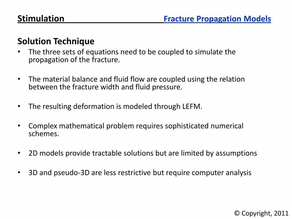
Solution Technique • The three sets of equations need to be coupled to simulate the
propagation of the fracture. • The material balance and fluid flow are coupled using the relation
between the fracture width and fluid pressure. • The resulting deformation is modeled through LEFM. • Complex mathematical problem requires sophisticated numerical
schemes. • 2D models provide tractable solutions but are limited by assumptions • 3D and pseudo-3D are less restrictive but require computer analysis
© Copyright, 2011
Stimulation Fracture Propagation Models
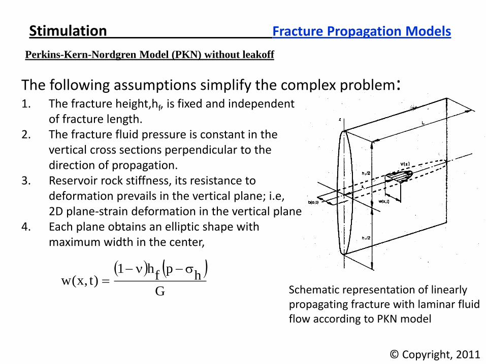
The following assumptions simplify the complex problem: 1. The fracture height,hf, is fixed and independent of fracture length. 2. The fracture fluid pressure is constant in the vertical cross sections perpendicular to the direction of propagation. 3. Reservoir rock stiffness, its resistance to deformation prevails in the vertical plane; i.e, 2D plane-strain deformation in the vertical plane 4. Each plane obtains an elliptic shape with maximum width in the center,
Perkins-Kern-Nordgren Model (PKN) without leakoff
Schematic representation of linearly propagating fracture with laminar fluid flow according to PKN model
G
hp
fh1
)t,x(w
© Copyright, 2011
Stimulation Fracture Propagation Models
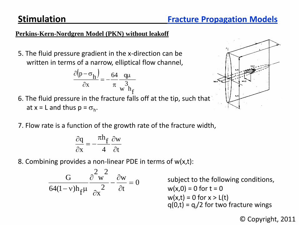
5. The fluid pressure gradient in the x-direction can be written in terms of a narrow, elliptical flow channel, 6. The fluid pressure in the fracture falls off at the tip, such that at x = L and thus p = h. 7. Flow rate is a function of the growth rate of the fracture width, 8. Combining provides a non-linear PDE in terms of w(x,t): subject to the following conditions, w(x,0) = 0 for t = 0 w(x,t) = 0 for x > L(t)
q(0,t) = qi/2 for two fracture wings
Perkins-Kern-Nordgren Model (PKN) without leakoff
fh
3w
q64
x
hp
t
w
4
fh
x
q
0t
w
2x
2w
2
fh)1(64
G
© Copyright, 2011

Stimulation Fracture Propagation Models
Assumptions: 1. Fixed fracture height, hf.
2. Rock stiffness is taken into account in the horizontal plane only. 2D plane strain deformation in the horizontal plane.
3. Thus fracture width does not depend on fracture
height and is constant in the vertical direction.
4. The fluid pressure gradient is with respect to a
narrow, rectangular slit of variable width,
Geertsma-de Klerk (GDK) Model without leakoff
Schematic representation of linearly propagating fracture with laminar fluid flow according to GDK model
x
0 )t,x(3
w
dx
fh
iq12
)t,x(p)t,0(p
© Copyright, 2011
Stimulation Fracture Propagation Models
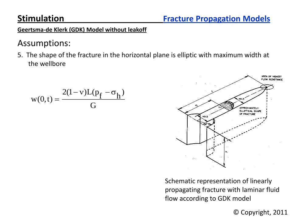
Assumptions: 5. The shape of the fracture in the horizontal plane is elliptic with maximum width at
the wellbore
Geertsma-de Klerk (GDK) Model without leakoff
Schematic representation of linearly propagating fracture with laminar fluid flow according to GDK model
G
)hf
p(L)1(2)t,0(w
© Copyright, 2011

Stimulation Fracture Propagation Models
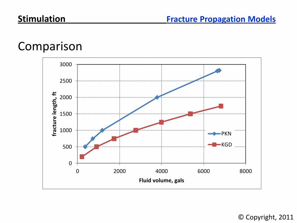
Comparison
0
100
200
300
400
500
600
700
800
900
1000
0 2000 4000 6000 8000
Ne
t p
ress
ure
at
we
llbo
re, p
si
Fluid volume, gals
PKN
KGD
© Copyright, 2011
Stimulation Fracture Propagation Models
Comparison
0
500
1000
1500
2000
2500
3000
0 2000 4000 6000 8000
frac
ture
len
gth
, ft
Fluid volume, gals
PKN
KGD
© Copyright, 2011
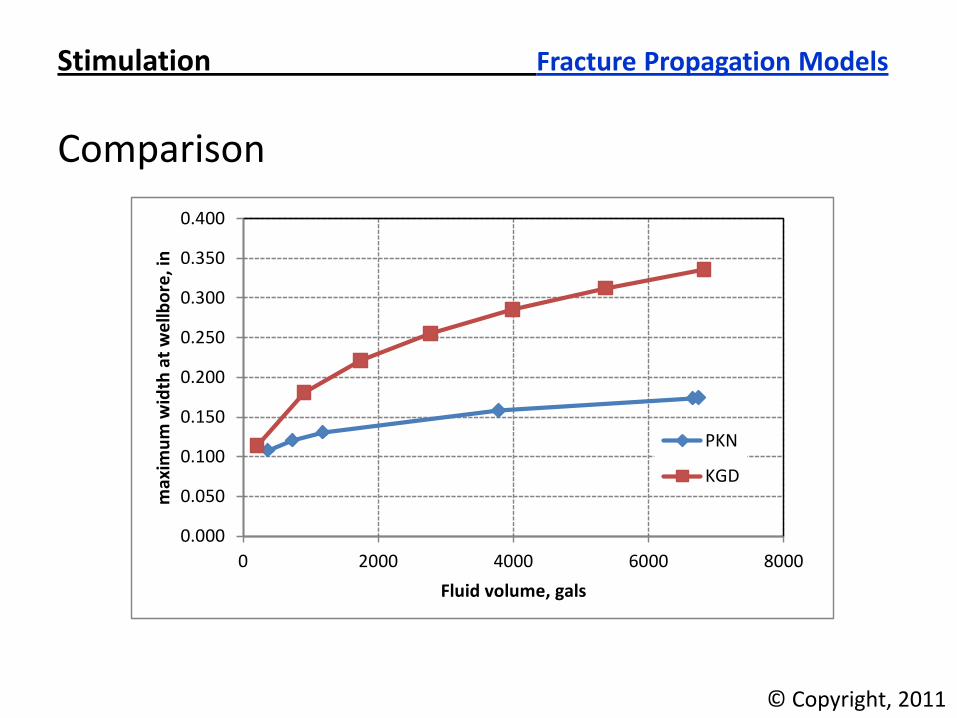
Stimulation Fracture Propagation Models
Comparison
0.000
0.050
0.100
0.150
0.200
0.250
0.300
0.350
0.400
0 2000 4000 6000 8000
max
imu
m w
idth
at
we
llbo
re, i
n
Fluid volume, gals
PKN
KGD
© Copyright, 2011

Stimulation 3D Fracture Propagation Models
Applications
• Primarily for complex reservoir conditions – Multiple zones with varying elastic or leakoff properties
– Closure stress profiles indicate complex geometries
Vertical fracture profile illustrating the changes in width across the fracture
© Copyright, 2011

Stimulation 3D Fracture Propagation Models
Components Assumptions 1. 3D stress distribution linear elastic behavior
propagation criterion given by fracture toughness
2. 2D fluid flow in fracture laminar flow of newtonian or non-newtonian fluid
3. 2D proppant transport
4. Heat transfer
5. Leakoff Leakoff is 1D, to fracture face
© Copyright, 2011
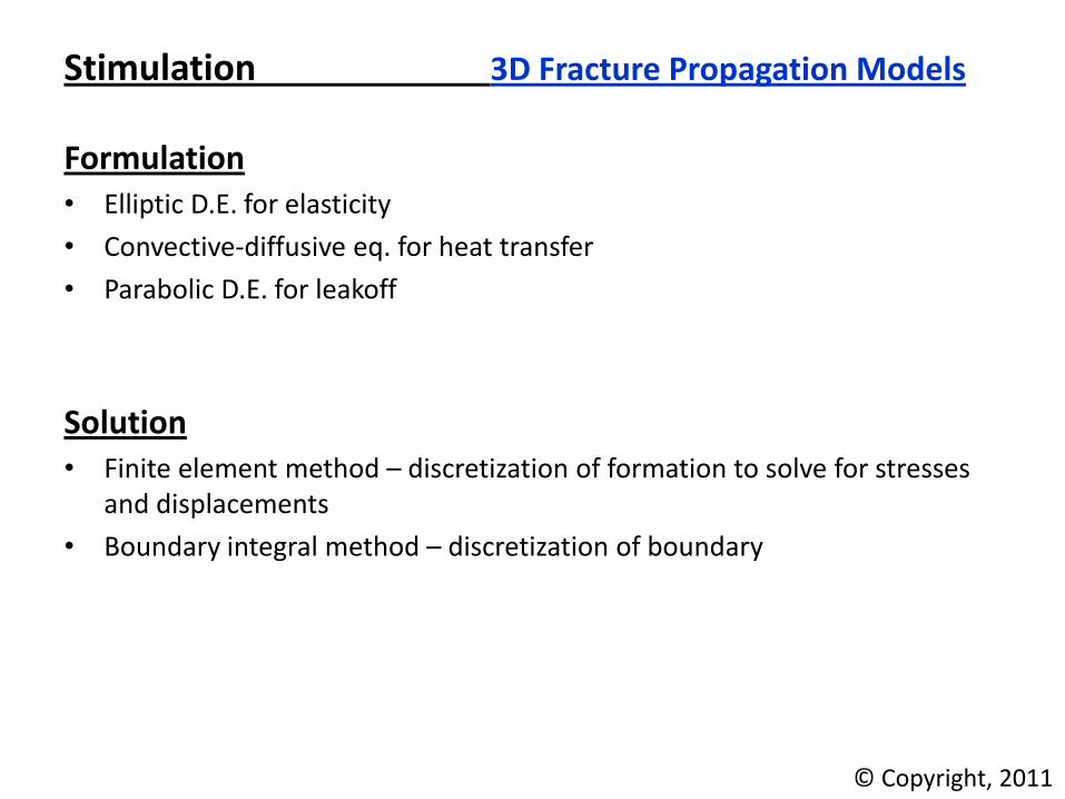
Stimulation 3D Fracture Propagation Models
Formulation • Elliptic D.E. for elasticity
• Convective-diffusive eq. for heat transfer
• Parabolic D.E. for leakoff
Solution • Finite element method – discretization of formation to solve for stresses
and displacements
• Boundary integral method – discretization of boundary
© Copyright, 2011
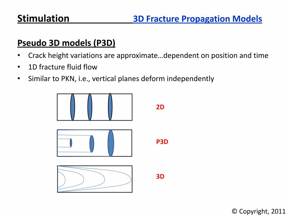
Stimulation 3D Fracture Propagation Models
Pseudo 3D models (P3D) • Crack height variations are approximate…dependent on position and time
• 1D fracture fluid flow
• Similar to PKN, i.e., vertical planes deform independently
2D P3D 3D
© Copyright, 2011

• Comparison to validate 2D models
• Example A: Strong stress barriers, negligible leakoff
• More examples in Chapter 5 of SPE monograph Vol 12
Stimulation 3D Fracture Propagation Models
3D simulator
Stimulation Fracture Propagation Models
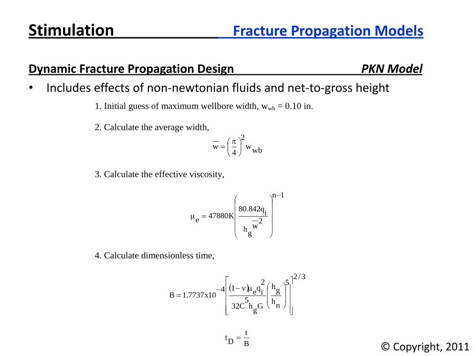
Dynamic Fracture Propagation Design PKN Model
• Includes effects of non-newtonian fluids and net-to-gross height
1. Initial guess of maximum wellbore width, wwb = 0.10 in.
2. Calculate the average width,
wbw
2
4w
3. Calculate the effective viscosity,
1n
2w
gh
iq842.80
K47880e
4. Calculate dimensionless time,
3/2
5
nh
gh
Gg
h5
C32
2
iq
e14
10x7737.1B
B
t
Dt
© Copyright, 2011
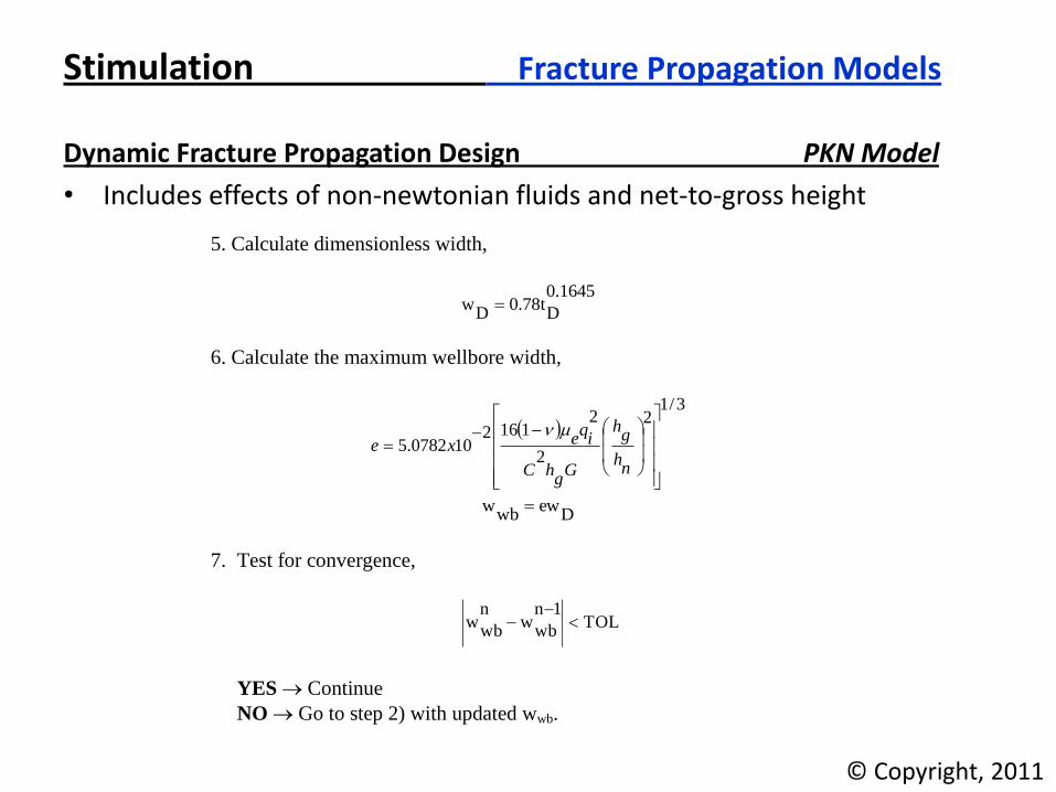
Stimulation Fracture Propagation Models
Dynamic Fracture Propagation Design PKN Model
• Includes effects of non-newtonian fluids and net-to-gross height
5. Calculate dimensionless width,
1645.0
Dt78.0
Dw
6. Calculate the maximum wellbore width,
3/1
2
2
21162
100782.5
nh
gh
Gg
hC
iq
exe
Dew
wbw
7. Test for convergence,
TOL1n
wbw
n
wbw
YES Continue
NO Go to step 2) with updated wwb.
© Copyright, 2011

Stimulation Fracture Propagation Models
Dynamic Fracture Propagation Design PKN Model
• Includes effects of non-newtonian fluids and net-to-gross height
8. Calculate the fracture length,
3/1
8
48256
512
104768.7
nh
gh
Gg
hC
iq
exa
6295.
Dt5809.0
DL
DaLL
1. Calculate the fracture volume,
12
Lg
hwV
10. Calculate the fracture pressure
min,h
4/1
31
Lei
q3
G
gh
02975.0)t,0(
fP
11. Update pumping time and repeat the procedure, starting at step 1).
© Copyright, 2011
Stimulation Fracture Propagation Models
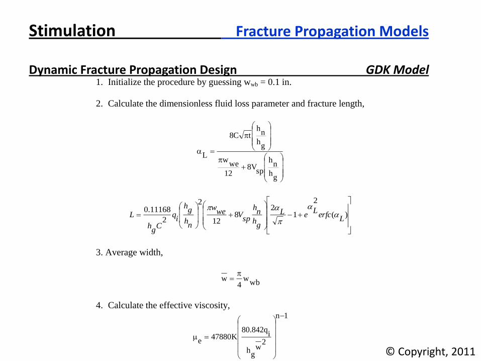
Dynamic Fracture Propagation Design GDK Model
1. Initialize the procedure by guessing wwb = 0.1 in.
2. Calculate the dimensionless fluid loss parameter and fracture length,
gh
nh
spV8
12
wew
gh
nh
tC8
L
)(
2
12
812
2
2
11168.0L
erfcL
eL
gh
nh
spVwe
w
nh
gh
iq
Cg
h
L
3. Average width,
wbw
4w
4. Calculate the effective viscosity, 1n
2w
gh
iq842.80
K47880e
© Copyright, 2011

Stimulation Fracture Propagation Models
Dynamic Fracture Propagation Design GDK Model
5. Simplified expression for fracture width,
4/1
gGh
2L
iq
e)1(84
1295.0wb
w
6. Test for convergence,
TOL1n
wbw
n
wbw
YES Continue
NO Go to step 2) with updated wwb.
7. Volume of one wing of the fracture,
48
wbhLw
V
8. Bottomhole fracture pressure,
min,
4/1
231
33
2
03725.0),0(
hL
gh
eiqG
gh
tf
P
9.Update pumping time and repeat the procedure, starting at step 1).
© Copyright, 2011

Stimulation Fracture Propagation Models
Nomenclature
a = length constant, ft.
B = time constant, min.
C = fluid loss coefficient, ft/(min)1/2
E = width constant, in.
G = shear modulus, psi
hg = gross fracture height, ft.
hn = net permeable sand thickness, ft.
K = consistency index, (lbf-secn)/ft
2
L = fracture length, ft.
LD = dimensionless fracture length
Pf = bottomhole fracture pressure, psi
qi = flow rate into single wing of fracture, bpm
t = pumping time, min.
tD = dimensionless time
V = volume of single wing, ft3
Vsp = spurt loss, ft3/ft
2
w = volumetric average fracture width, in.
wD = dimensionless fracture width
wwb = fracture width at wellbore, in.
wwe = fracture width at wellbore at end of pumping, in.
L = dimensionless fluid-loss parameter including spurt loss
e = effective fracture fluid viscosity, cp
h = horizontal, minimum stress, psi
= poisson’s ratio
© Copyright, 2011