The moving bottleneck problem: a Hamilton-Jacobi approach moving bottleneck problem: a Hamilton-Jacobi approach ... (1963), Makigami et al(1971), Laval and Leclercq ... The moving

The moving bottleneck problem:

a Hamilton-Jacobi approach

Guillaume Costesequein collaboration with Aurelien Duret

Inria Sophia-Antipolis Mediterranee& Universite de Lyon, IFSTTAR-ENTPE

TRAM3 Terminus Meeting 2016, Sophia-AntipolisJanuary 07, 2016

G. Costeseque (Inria) Moving Bottleneck & HJ equations Valbonne, Jan. 07 2016 1 / 42

Motivation

Example

Congested off-ramp

[Richmond Bridge, c©Bay Area Council]

Traffic flow model for the upstream section?


Motivation

Outline

1 Introduction to traffic

2 The moving bottleneck theory

3 Mesoscopic formulation of multiclass multilane models

4 Numerical scheme

5 Conclusion and perspectives


Introduction to traffic

Outline




4 Numerical scheme



Introduction to traffic Macroscopic models

Convention for vehicle labeling

N

x

t

Flow



Three representations of traffic flow

Moskowitz’ surface

Flow x

t

N

x

See also [Moskowitz and Newman(1963), Makigami et al(1971), Laval and

Leclercq(2013)]



Notations(macroscopic)

N(t, x) vehicle label at (t, x)

the flow q(t, x) = lim∆t→0

N(t +∆t, x)− N(t, x)

∆t,

x

N(x , t ±∆t)

the density ρ(t, x) = lim∆x→0

N(t, x) − N(t, x +∆x)

∆x,

x

∆x

N(x ±∆x , t)

the stream speed (mean spatial speed) V (t, x).


Introduction to traffic Focus on LWR model

First order: the LWR model

LWR model [Lighthill and Whitham, 1955], [Richards, 1956]

Scalar one dimensional conservation law

∂tρ+ ∂xQ (ρ) = 0, (t, x) ∈ (0,+∞) × R (1)

withQ : ρ 7→ q =: Q (ρ)


Introduction to traffic Focus on LWR model

Overview: conservation laws (CL) / Hamilton-Jacobi (HJ)

Eulerian Lagrangiant − x t − n

CLVariable Density ρ Spacing r := 1

ρ

Equation ∂tρ+ ∂xQ(ρ) = 0 ∂t r + ∂nV (r) = 0

HJ

Variable Label N Position X

N(t, x) =

∫ +∞

x

ρ(t, ξ)dξ X (t, n) =

∫ +∞

n

r(t, η)dη

Equation ∂tN − Q (−∂xN) = 0 ∂tX − V (−∂nX ) = 0


Introduction to traffic Mesoscopic resolution

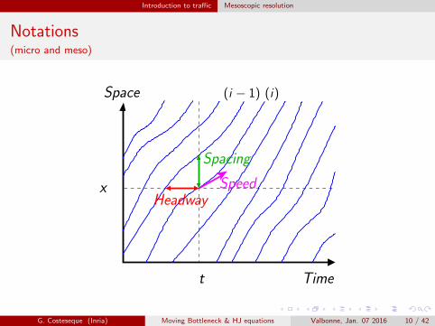
Notations(micro and meso)

Speed

Time

(i − 1)Space

x

Spacing

Headway

t

(i)



Mesoscopic resolution of the LWR model

Speed

Time

(i − 1)Space

x

Spacing

Headway

t

(i) Introduce

the pace p :=1

vthe headway h = H(p)

the passing time

T (n, x) :=

∫ x

−∞

p(n, ξ)dξ.

{

∂nT = h, (headway)

∂xT = p, (pace)

[Leclercq and Becarie(2012), Laval and Leclercq(2013)]



Mesoscopic resolution of the LWR model(Continued)

Lagrangian-spacen− x

CLVariable Pace p

Equation ∂np − ∂xH(p) = 0

HJ

Variable Passing time T

T (n, x) =

∫ x

−∞

p(n, ξ)dξ

Equation ∂nT − H (∂xT ) = 0



Lax-Hopf formula

1

u

H

p

1

κ

1

C

1

wκ

Assume

H(r) =

1

κr +

1

wκ, if r ≥

1

u,

+∞, otherwise,

Proposition (Representation formula (Lax-Hopf))

The solution under smooth boundary conditions is given by

T (n, x) = max{

T (n, 0) +x

u︸︷︷︸

= free flow

, T(

0, x +n

κ

)

+n

wκ︸︷︷︸

= congested

}

. (2)

See [Laval and Leclercq(2013)]G. Costeseque (Inria) Moving Bottleneck & HJ equations Valbonne, Jan. 07 2016 13 / 42


Lax-Hopf formula

0

1

κ

x

n

n

x T (n, x)

T (n, 0)

T (0, x)



Dynamic programming

n

x +∆x

x −∆x

n −∆n

x

1

κ

x

n

∆x

∆n

T (n, x)

Introduce a grid with steps(∆n,∆x) satisfying

∆n = κ∆x



Mesoscopic: what for?

Strengths1 Consistent with micro and macro representations2 Large scale networks // spatial discontinuities OK3 Data assimilation (from Eulerian and Lagrangian sensors)

Weakness1 Single pipe2 Mono class3 No capacity drop at junctions

Developments1 Multilane and multiclass approach2 Friction term

−→ Moving bottleneck theory


The moving bottleneck theory

Outline




4 Numerical scheme




Some definitionsFollowing [Gazis and Herman(1992), Newell(1998), Laval and Leclercq(2013)],

Definition

A moving bottleneck (MB) is defined as a vehicle with a maximal free flowspeed strictly lower than the free flow speed of its immediate followingvehicle.

A moving bottleneck is said to be active if and only if it generates queuesat upstream positions with respect to the moving bottleneck and if theupstream state is different from the downstream state.

The passing rate is the maximal flow that can overtake the movingbottleneck in the Eulerian framework.



Notations

vB

−w

−w

vB

k

Q

(N − 1) lanes N lanes

R(vB , qD)

(D) (U)

ξN(t)

x

(U) (D)

vB

kD (N − 1)κ Nκ

qD

NC

Q∗(vB)

u



Notations

vB

−w

−w

vB

k

Q

(N − 1) lanes N lanes

R(vB , qD)

(D) (U)

ξN(t)

x

(U) (D)

vB

kD (N − 1)κ Nκ

qD

NC

Q∗(vB)

u

ξN(t) = trajectory of the MB in t − x

ξT (n) = location where the vehicle ncrosses the MB

vB(t) := ξN(t) MB speed

kD := k (t, ξN(t)+) downstream

density,

qD := Q(kD) downstream flow,

R(vB , qD) = passing rate

R(vB , qD) := qD − kDvB



Math problem in Eulerian framework

Coupled ODE-PDE problem on [0,+∞)× R

∂tk + ∂x (Q(k)) = 0,

Q(k(t, ξN(t)))− ξN(t)k(t, ξN(t)) ≤N − 1

NQ∗

(

ξN(t))

,

ξN(t) = min {vb, V (k(t, ξN(t)+))} ,

(3)

with {

k(0, x) = k0(x), on R,

ξN(0) = ξ0.(4)

Theorem (Existence result [Delle Monache and Goatin(2014)])

For BV initial data, there exist weak solutions of (3)-(4).Uniqueness is still an open problem.



Interpretation

Remark

Upper bound on the passing rate in (3) depends on the moving bottleneckspeed

vB(t) 7→ Q∗(vB(t))

and it is the Legendre-Fenchel transform of the flow-density FD Q

Q∗(v) := supρ∈Dom(Q)

{Q(ρ)− vρ} .


Mesoscopic formulation of multiclass multilane models

Outline




4 Numerical scheme




Stretch of road [x0, x1] composed by N separate lanes

Two classes of users: “rabbits” (I = 1) and “slugs” (I = 2).

Class-dependent Hamiltonian

H : (r , I ) 7→ H(r , I )

for a given class attribute I ∈ {1, 2}



Stretch of road [x0, x1] composed by N separate lanes

Two classes of users: “rabbits” (I = 1) and “slugs” (I = 2).

Class-dependent Hamiltonian

H : (r , I ) 7→ H(r , I )

for a given class attribute I ∈ {1, 2}

If triangular, then u1 > u2

0 0.02 0.04 0.06 0.08 0.1 0.12 0.14 0.16 0.18 0.2Density (veh/m)

0

0.1

0.2

0.3

0.4

0.5

0.6

0.7

0.8

Flo

w (

veh/

s)

Fundamental Diagrams

RabbitsSlugs


Mesoscopic formulation of multiclass multilane models Capacity drop

Capacity drop parameter

(U)(D)

(U)Case FIFOCase non−FIFO

(U) (D)

Flow

(MB)

vB

R(vB , qD)

δ = 1δ = 0

r

H

1

κ

1

urB =

1

vB

hB =1

qD

1

R(vB , qD)

vB

1

C1

wκ

Introduce parameter δ ∈ [0, 1]

If δ = 0, strictly non-FIFO

If 0 < δ < 1, reduction of theresidual headway on the passinglane(s)

If δ = 1, strictly FIFO



Illustration of the capacity drop effect

Link composed of two lanesA single vehicle from class 2 (MB)No capacity drop occurs δ = 0

Time (s)40 60 80 100 120 140 160 180

Spa

ce (

m)

0

100

200

300

400

500

600

700

800

900

1000

Trajectories

T2(n, x)

T1(n, x)



Time (s)40 60 80 100 120 140 160 180

Spa

ce (

m)

0

100

200

300

400

500

600

700

800

900

1000

Trajectories

T2(n, x)

T1(n, x)

Time (s)40 60 80 100 120 140 160 180

Spa

ce (

m)

0

100

200

300

400

500

600

700

800

900

1000

Trajectories

T2(n, x)

T1(n, x)

δ = 1 δ = 0.6

Time (s)40 60 80 100 120 140 160 180

Spa

ce (

m)

0

100

200

300

400

500

600

700

800

900

1000

Trajectories

T2(n, x)

T1(n, x)

Time (s)40 60 80 100 120 140 160 180

Spa

ce (

m)

0

100

200

300

400

500

600

700

800

900

1000

Trajectories

T2(n, x)

T1(n, x)

δ = 0.4 δ = 0.2


Mesoscopic formulation of multiclass multilane models Expression of the MCML model

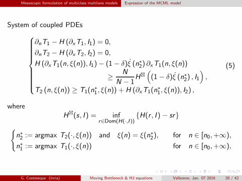
System of coupled PDEs

∂nT1 − H (∂xT1, I1) = 0,

∂nT2 − H (∂xT2, I2) = 0,

H (∂xT1(n, ξ(n)), I1)− (1− δ)ξ (n∗2) ∂xT1(n, ξ(n))

≥N

N − 1H⊠

(

(1− δ)ξ (n∗2) , I1

)

,

T2 (n, ξ(n)) ≥ T1(n∗

1, ξ(n)) + H (∂xT1(n∗

1, ξ(n)), I2) ,

(5)

whereH⊠(s, I ) = inf

r∈Dom(H(·,I )){H(r , I ) − sr}

{

n∗2 := argmax T2(·, ξ(n)) and ξ(n) = ξ(n∗2), for n ∈ [n0,+∞),

n∗1 := argmax T1(·, ξ(n)) for n ∈ [n0,+∞),



+ mixed Neumann-Dirichlet boundary conditions

∂nTi (n, x0) = gi (n), on [n0,+∞),

∂nTi (n, x1) = gi (n), on [n0,+∞),

Ti (n0, x) = Gi(x), on [x0, x1],

for i ∈ {1, 2} . (6)

x

nn0

x1

x0

Downstream Supply

Upstream Demand

First trajectory



Assumptions

1

ur

1

(N − 1)κ

ξ(n∗2) ξ(n∗2)

N lanes

(N − 1) lanes

1

Nκ

hB =1

(N − 1)C

rB

1

NC

1

Nwκ

H∗(

ξ(n∗2))

hB −ξ(n∗2)

u

H

n∗i (i ∈ {1, 2}: the nearestleader from class i for vehicle nof class j 6= i

Modified passing headway H

H =1

1− δhB −

ξT (n∗2)

u1

where hB =1

(N − 1)Cis the

residual headway


Numerical scheme

Outline




4 Numerical scheme



Numerical scheme Setting of the IBV Problem

Finite steps (∆n,∆x) > 0

∆n = κ∆x .

Class-specific Hamiltonians H are triangular

H(r , Ii ) =

1

κN(Ii )

(

r +1

w

)

, if r ≥1

ui,

+∞, otherwise,

(7)

N(Ii ) stands for the number of lanes that are accessible for the class i

N(Ii ) :=

{

N, for i = 1,

1, for i = 2.


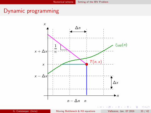
Numerical scheme Setting of the IBV Problem

Dynamic programming

∆n

n

x +∆x

x −∆x

n −∆n

x

1

κ

T (n, x)

ξMB(n)

∆x

x

n


Numerical scheme Lax-Hopf formulæ for the MCML model

Representation formulæ

For any (n, x) ∈ [n0, nmax ]× [x0, x1],

T1(n, x) = max

{

T1(n, x −∆x) +∆x

u1,T1(n −∆n, x +∆x) +

∆x

w

}

,

T2(n, x) = max

{

T2(n, x −∆x) +∆x

u2, T2(n −∆n, x +∆x) +

∆x

w

}

(8)


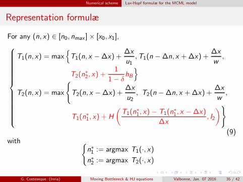
Numerical scheme Lax-Hopf formulæ for the MCML model

Representation formulæ

For any (n, x) ∈ [n0, nmax ]× [x0, x1],

T1(n, x) = max{

T1(n, x −∆x) +∆x

u1,T1(n −∆n, x +∆x) +

∆x

w,

T2(n∗

2, x) +1

1− δhB

}

T2(n, x) = max

{

T2(n, x −∆x) +∆x

u2, T2(n −∆n, x +∆x) +

∆x

w,

T1(n∗

1, x) + H

(T1(n

∗

1, x) − T1(n∗

1, x −∆x)

∆x, I2

)}

(9)with {

n∗1 := argmax T1(·, x)

n∗2 := argmax T2(·, x)


Numerical scheme Some mathematical results

Proposition (Existence of a continuous solution to (5)-(6))

Assume that r 7→ H (r , Ii ) is convex for any i ∈ {1, 2}. Then, the IBVproblem (5)-(6) admits a solution (T1,T2) continuous on[n0,+∞]× [x0, x1].

Proposition (Convergence)

Assume that r 7→ H (r , Ii ) is convex for any i ∈ {1, 2}. Then the numericalsolution (T ε

1 ,Tε

2 ) of the scheme (9) converges towards a continuoussolution (T1,T2) of the IBV problem (5)-(6) when ε := (∆n,∆x) goestoward zero.


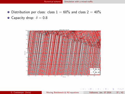
Numerical scheme Simulation with a mixed traffic

Distribution per class: class 1 = 60% and class 2 = 40%

Capacity drop: δ = 0.8

50 100 150 200 250 300 350 400 450 500 550Time (s)

0

100

200

300

400

500

600

700

800

900

1000

Spa

ce (

m)

(alpha, delta) = (0.6, 0.8)

T2(n, x)

T1(n, x)


Numerical scheme Simulation with a mixed traffic

20 40 60 80 100 120 140 160 180 200 220 240Vehicle label

40

60

80

100

120

140

160

180

Tra

vel t

ime

(s)

Class 1

20 40 60 80 100 120 140 160Vehicle label

40

60

80

100

120

140

160

180

Tra

vel t

ime

(s)

Class 2


Conclusion and perspectives

Outline




4 Numerical scheme



Conclusion and perspectives

A new event-based mesoscopic model for multi-class traffic flowmodeling on multi-lane sections

Theory of moving bottlenecks

Wide networks

Among the perspectives:

Well posedness

Sensitivity analysis (→ Regis’ presentation)

Validation with real traffic data

Data assimilation for real-time applications (→ Francesca’spresentation)


References

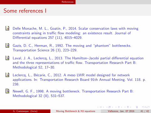
Some references I

Delle Monache, M. L., Goatin, P., 2014. Scalar conservation laws with movingconstraints arising in traffic flow modeling: an existence result. Journal ofDifferential equations 257 (11), 4015–4029.

Gazis, D. C., Herman, R., 1992. The moving and “phantom” bottlenecks.Transportation Science 26 (3), 223–229.

Laval, J. A., Leclercq, L., 2013. The Hamilton–Jacobi partial differential equationand the three representations of traffic flow. Transportation Research Part B:Methodological 52, 17–30.

Leclercq, L., Becarie, C., 2012. A meso LWR model designed for networkapplications. In: Transportation Research Board 91th Annual Meeting. Vol. 118. p.238.

Newell, G. F., 1998. A moving bottleneck. Transportation Research Part B:Methodological 32 (8), 531–537.


References

Thanks for your attention

Any question?

[email protected]


mailto:[email protected]

Documents

The moving bottleneck problem: a Hamilton-Jacobi approach moving bottleneck problem: a Hamilton-Jacobi approach ... (1963), Makigami et al(1971), Laval and Leclercq ... The moving