Embed Size (px)
Citation preview
The Multi-Layer Perceptron
non-linear modelling by adaptive pre-processing
Rob HarrisonAC&SE
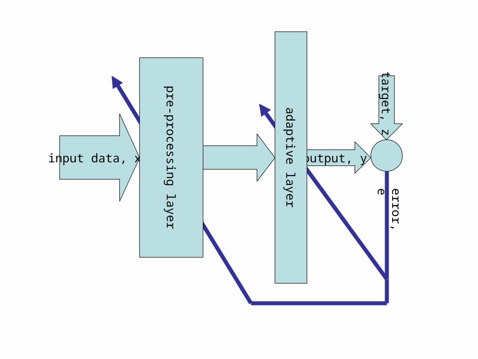
error, e
input data, x output, y
adaptive layer
target, z
pre-processing layer
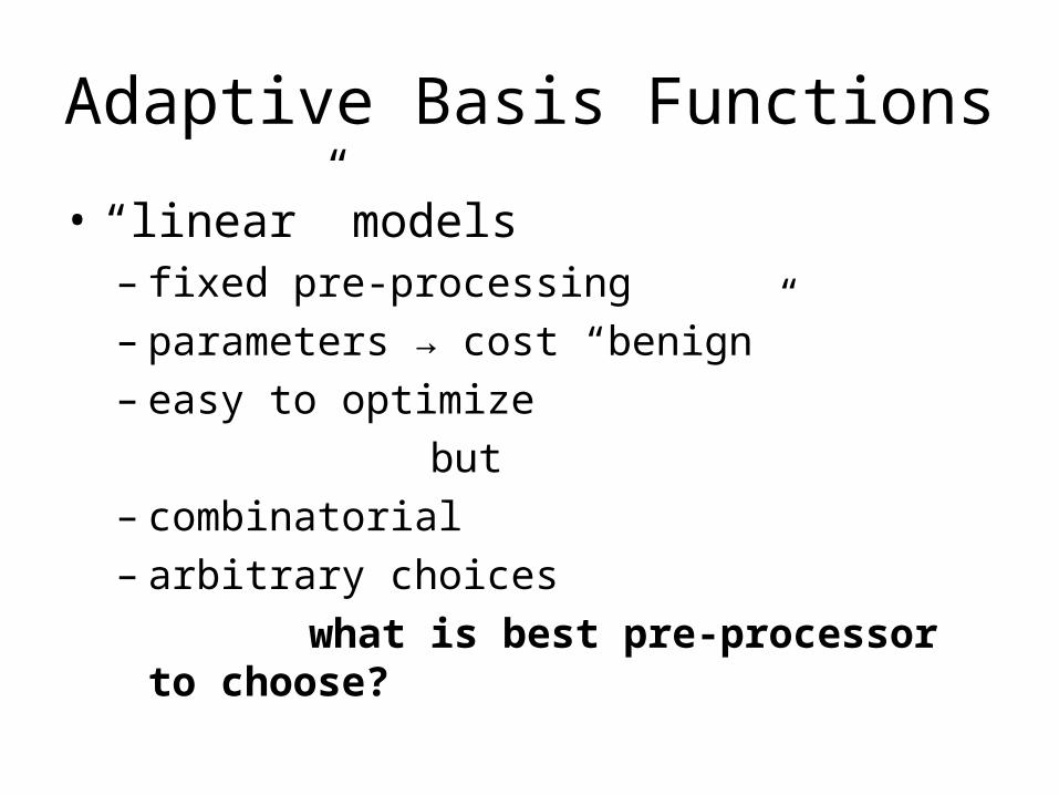
Adaptive Basis Functions
• “linear” models– fixed pre-processing– parameters → cost “benign”– easy to optimize
but– combinatorial– arbitrary choices
what is best pre-processor to choose?
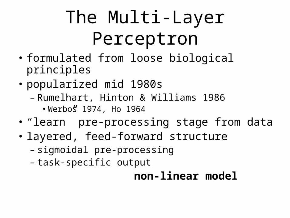
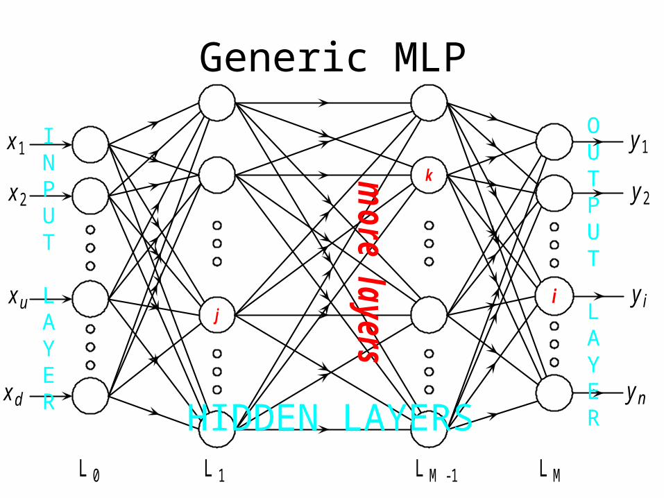
The Multi-Layer Perceptron
• formulated from loose biological principles• popularized mid 1980s
– Rumelhart, Hinton & Williams 1986• Werbos 1974, Ho 1964
• “learn” pre-processing stage from data• layered, feed-forward structure
– sigmoidal pre-processing– task-specific output
non-linear model
j
k
i
x 1
x 2
x u
x d
y 1
y 2
y i
y n
L 0 L 1 LM -1 LM
more layers
Generic MLP
INPUT
LAYER
OUTPUT
LAYERHIDDEN LAYERS
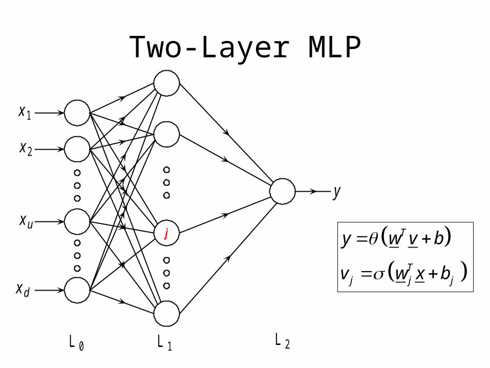
Two-Layer MLP
j
x 1
x 2
x u
x d
y
L 0 L 1 L 2
T
Tj j j
y w v b
v w x b
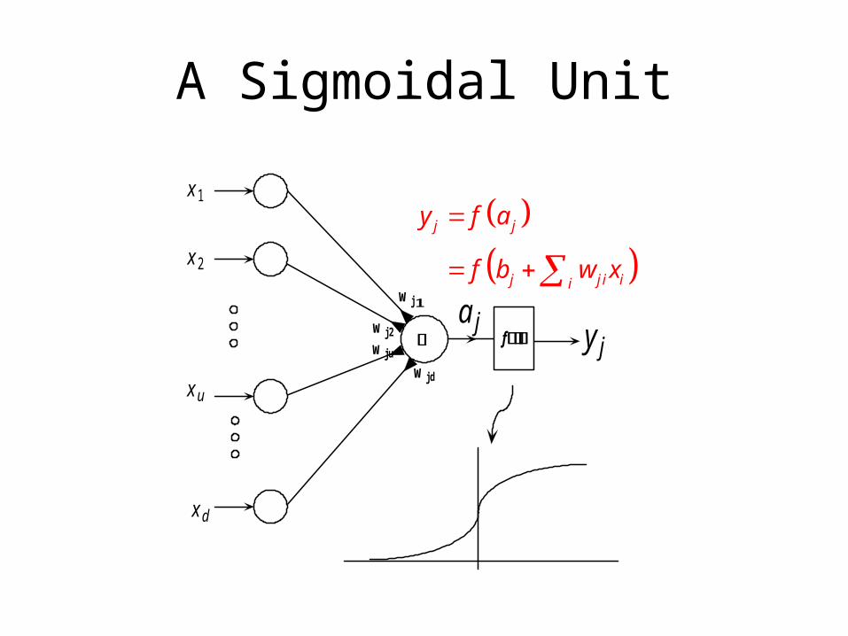
A Sigmoidal Unit
y j
x 1
x 2
x u
x d
fa j
w j
w j2
w ju
w jd
j j
j j i ii
y f a
f b w x
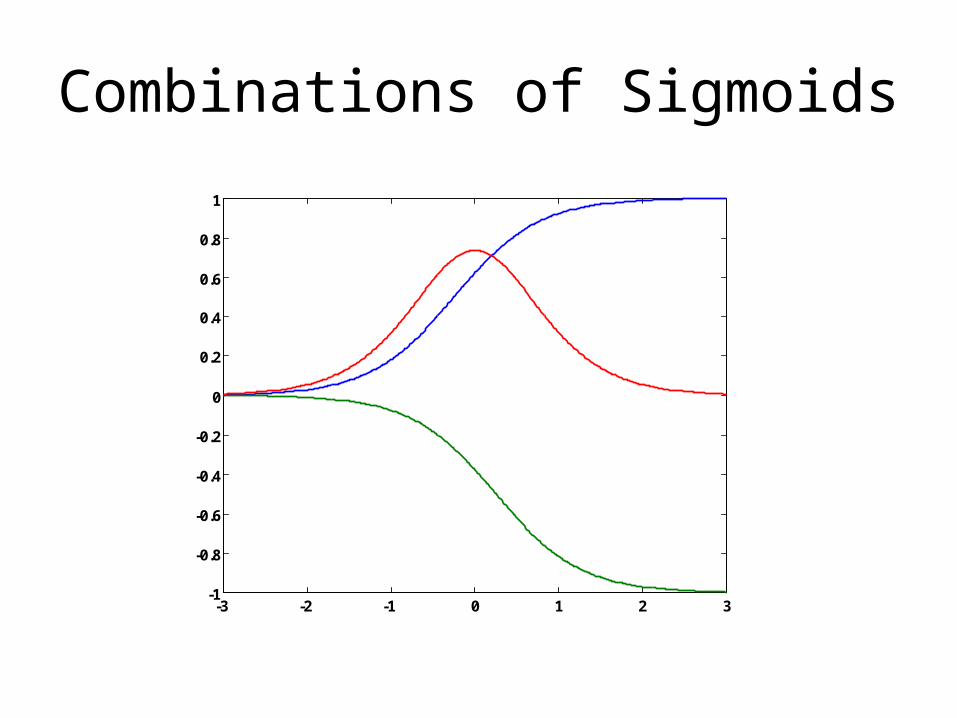
Combinations of Sigmoids
-3 -2 -1 0 1 2 3-1
-0.8
-0.6
-0.4
-0.2
0
0.2
0.4
0.6
0.8
1
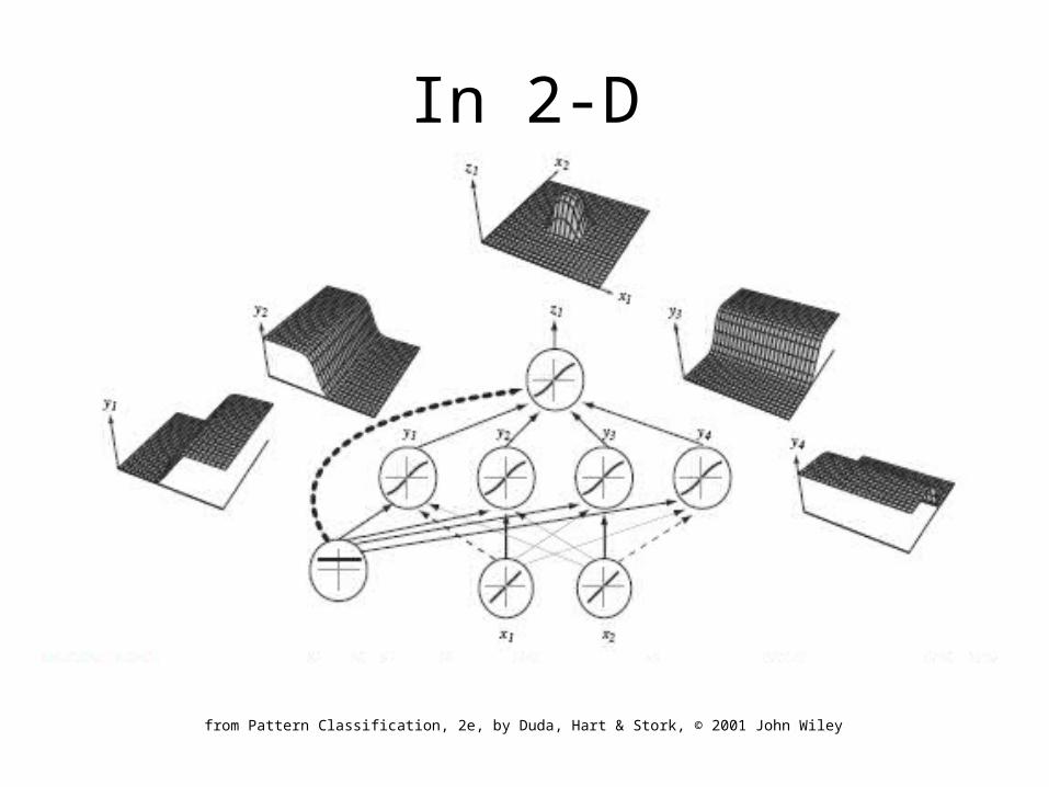
In 2-D
from Pattern Classification, 2e, by Duda, Hart & Stork, © 2001 John Wiley
Universal Approximation
• linear combination of “enough” sigmoids– Cybenko, 1990
• single hidden layer adequate– more may be better
• choose hidden parameters (w, b) optimally
problem solved?
Pros
• compactness– potential to obtain same veracity with much
smaller model
• c.f. sparsity/complexity control in linear models
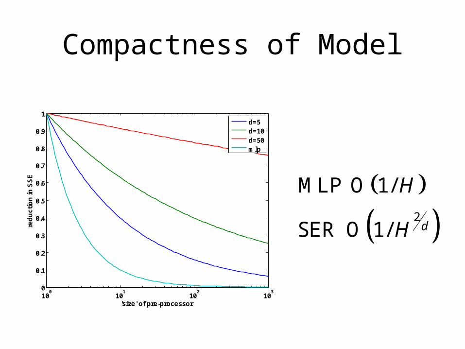
Compactness of Model
100
101
102
103
0
0.1
0.2
0.3
0.4
0.5
0.6
0.7
0.8
0.9
1
'size' of pre-processor
red
uc
tio
n i
n S
SE
d=5d=10d=50mlp
2
MLP 1/
SER 1/ d
H
H
O
O
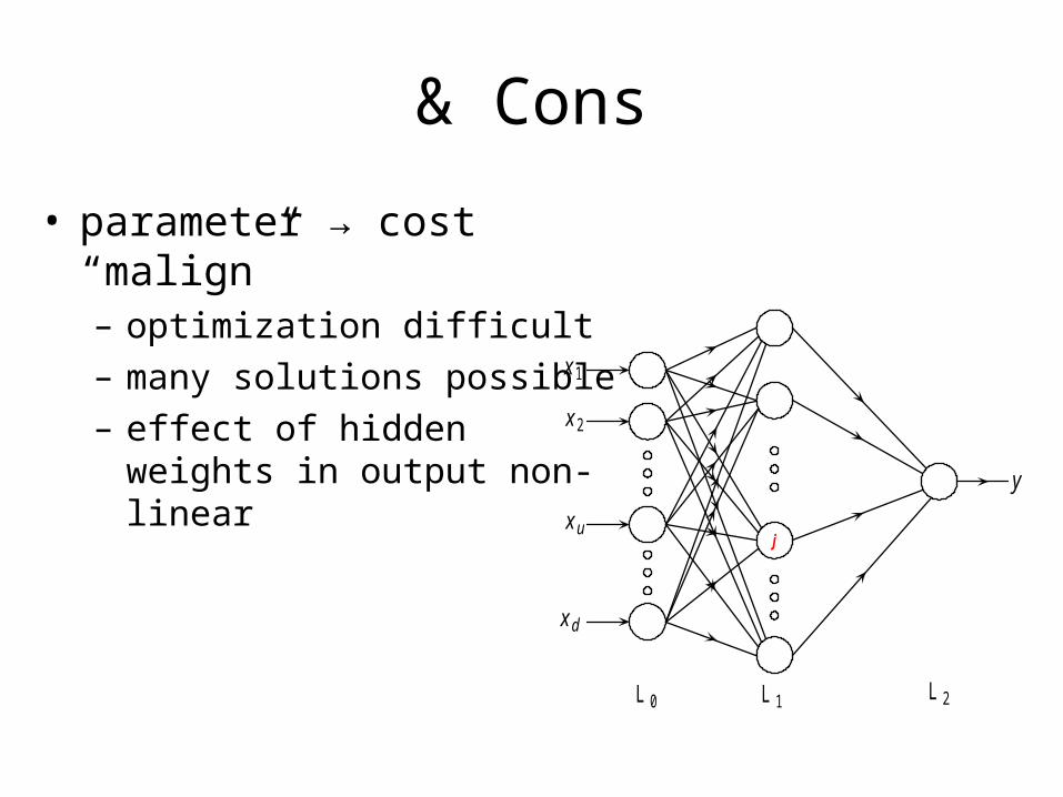
& Cons
• parameter → cost “malign”– optimization difficult– many solutions possible– effect of hidden weights in
output non-linear
j
x 1
x 2
x u
x d
y
L 0 L 1 L 2
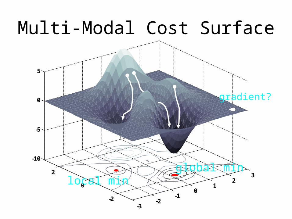
Multi-Modal Cost Surface
-3-2
-10
12
3
-2
0
2
-10
-5
0
5
global minlocal min
gradient?
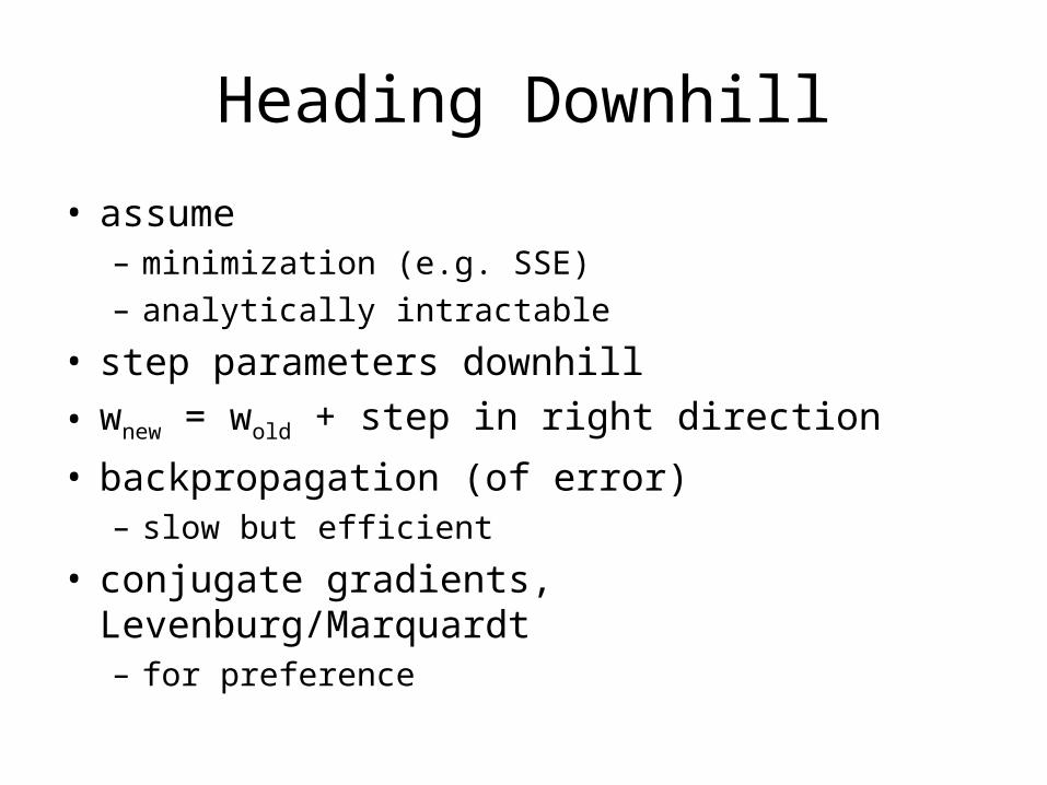
Heading Downhill
• assume– minimization (e.g. SSE)– analytically intractable
• step parameters downhill
• wnew = wold + step in right direction
• backpropagation (of error)– slow but efficient
• conjugate gradients, Levenburg/Marquardt– for preference
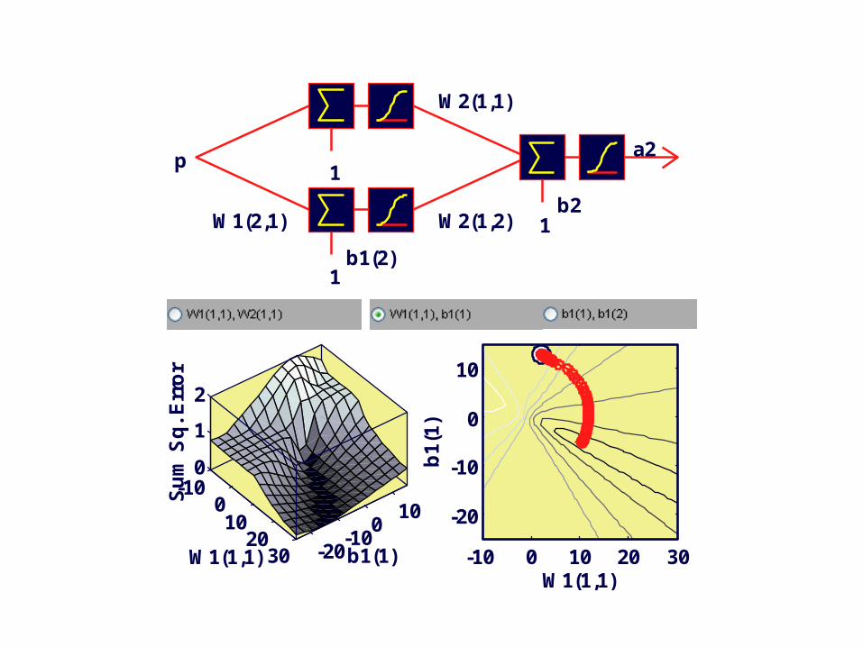
Neural NetworkDESIGNSteepest Descent Backprop #1
Use the radio buttonsto select the networkparameters to trainwith backpropagation.The correspondingerror surface andcontour are shownbelow.Click in the contourgraph (on the right)to start thesteepest descentlearning algorithm.
Chapter 12
p
W1(1,1)
1b1(1)
W1(2,1)
1b1(2)
W2(1,1)
W2(1,2) 1b2
a2
-10010
2030 -20
-100
10
0
1
2
b1(1)W1(1,1)
Su
m S
q.
Err
or
-10 0 10 20 30
-20
-10
0
10
W1(1,1)
b1
(1)
Neural NetworkDESIGNSteepest Descent Backprop #1
Use the radio buttonsto select the networkparameters to trainwith backpropagation.The correspondingerror surface andcontour are shownbelow.Click in the contourgraph (on the right)to start thesteepest descentlearning algorithm.
Chapter 12
p
W1(1,1)
1b1(1)
W1(2,1)
1b1(2)
W2(1,1)
W2(1,2) 1b2
a2
-10010
2030 -20
-100
10
0
1
2
b1(1)W1(1,1)
Su
m S
q. E
rro
r
-10 0 10 20 30
-20
-10
0
10
W1(1,1)
b1
(1)
Neural NetworkDESIGNConjugate Gradient Backprop
Use the radio buttonsto select the networkparameters to trainwith backpropagation.The correspondingcontour plot isshown to the left.Click in the contourgraph to start theconjugate gradientlearning algorithm.
Chapter 12-10 0 10 20 30-25
-20
-15
-10
-5
0
5
10
15
W1(1,1)
b1
(1)
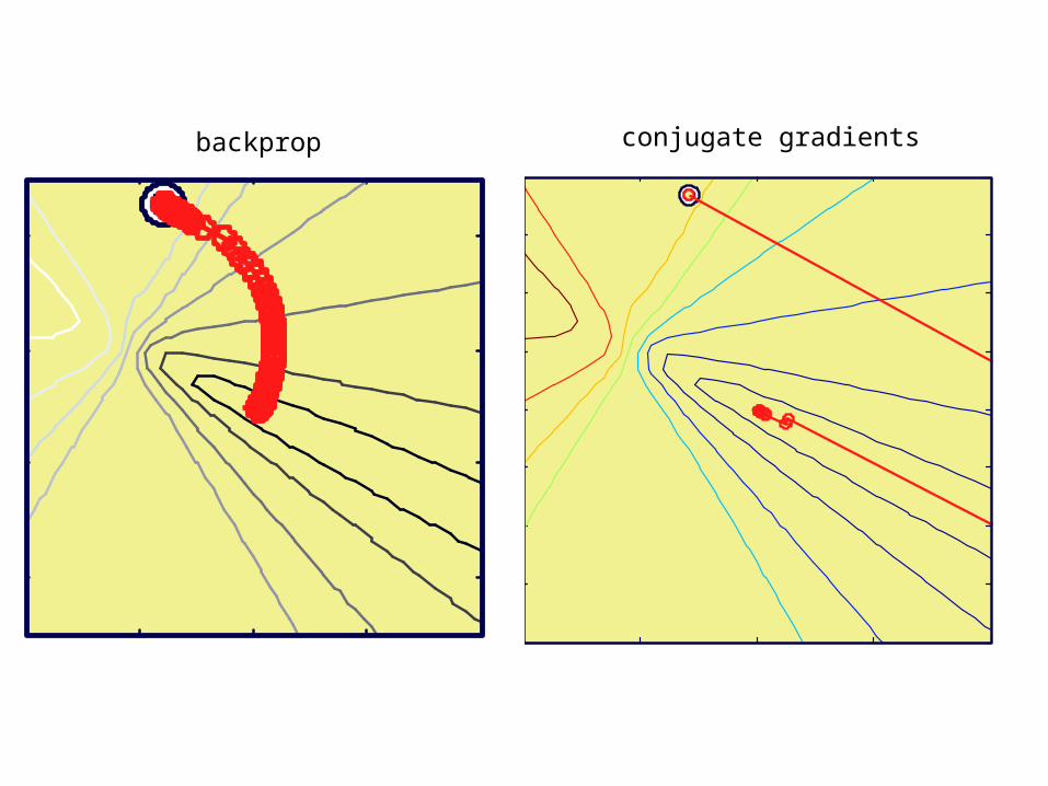
backprop conjugate gradients
Implications
• correct structure can get “wrong” answer– dependency on initial conditions– might be good enough
• train / test (cross-validation) required– is poor behaviour due to
• network structure?• ICs?
additional dimension in development
Is It a Problem?
• pros seem to outweigh cons
• good solutions often arrived at quickly
• all previous issues apply– sample density– sample distribution– lack of prior knowledge
How to Use
• to “generalize” a GLM– linear regression – curve-fitting
• linear output + SSE
– logistic regression – classification• logistic output + cross-entropy (deviance)• extend to multinomial, ordinal
– e.g. softmax outptut + cross entropy
– Poisson regression – count data
What is Learned?
• the right thing– in a maximum likelihood sense
theoretical
• conditional mean of target data, E(z|x)– implies probability of class membership for
classification P(Ci|x)
estimated
• if good estimate then y → E(z|x)
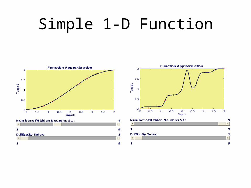
Simple 1-D Function
Neural Network DESIGN Generalization
Click the [Train]button to train thelogsig-linearnetwork on thedata points at left.
Use the slide barto choose thenumber of neuronsin the hidden layer.
Chapter 11
Number of Hidden Neurons S1: 4
1 9
Difficulty Index: 1
1 9
-2 -1.5 -1 -0.5 0 0.5 1 1.5 20
0.5
1
1.5
2
Input
Targ
et
Function Approximation
Neural Network DESIGN Generalization
Click the [Train]button to train thelogsig-linearnetwork on thedata points at left.
Use the slide barto choose thenumber of neuronsin the hidden layer.
Chapter 11
Number of Hidden Neurons S1: 9
1 9
Difficulty Index: 1
1 9
-2 -1.5 -1 -0.5 0 0.5 1 1.5 20
0.5
1
1.5
2
Input
Targ
et
Function Approximation
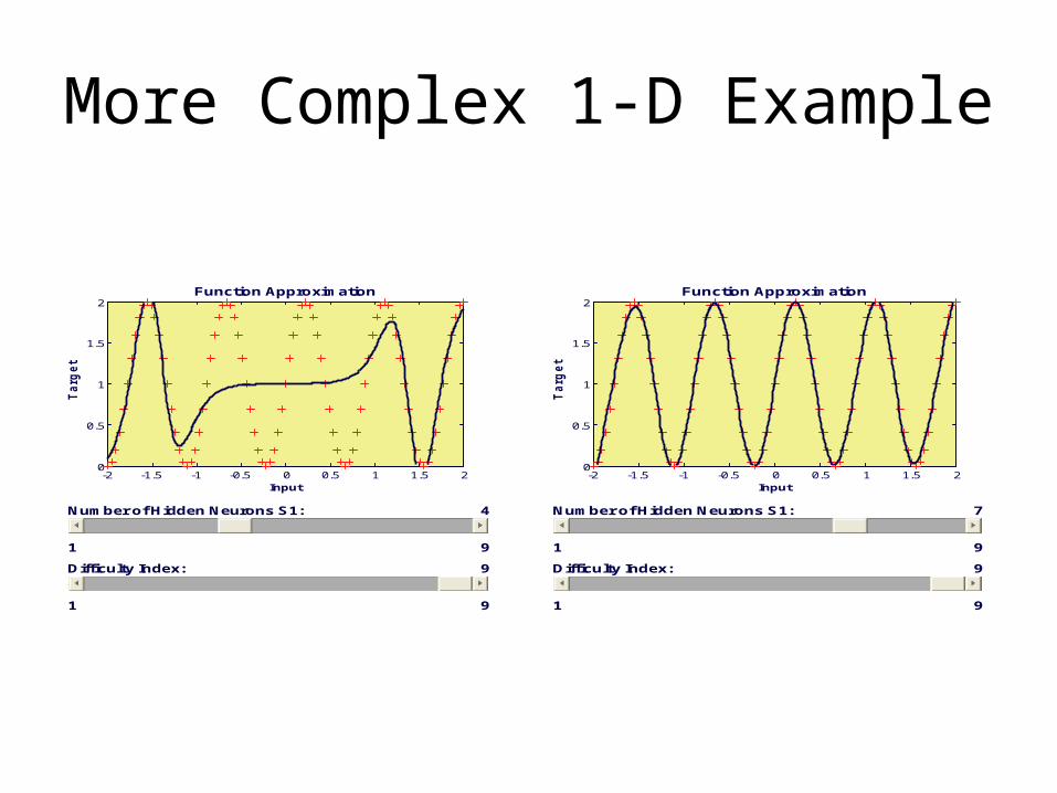
More Complex 1-D Example
Neural Network DESIGN Generalization
Click the [Train]button to train thelogsig-linearnetwork on thedata points at left.
Use the slide barto choose thenumber of neuronsin the hidden layer.
Chapter 11
Number of Hidden Neurons S1: 4
1 9
Difficulty Index: 9
1 9
-2 -1.5 -1 -0.5 0 0.5 1 1.5 20
0.5
1
1.5
2
Input
Targ
et
Function Approximation
Neural Network DESIGN Generalization
Click the [Train]button to train thelogsig-linearnetwork on thedata points at left.
Use the slide barto choose thenumber of neuronsin the hidden layer.
Chapter 11
Number of Hidden Neurons S1: 7
1 9
Difficulty Index: 9
1 9
-2 -1.5 -1 -0.5 0 0.5 1 1.5 20
0.5
1
1.5
2
Input
Targ
et
Function Approximation
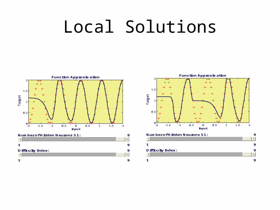
Local Solutions
Neural Network DESIGN Generalization
Click the [Train]button to train thelogsig-linearnetwork on thedata points at left.
Use the slide barto choose thenumber of neuronsin the hidden layer.
Chapter 11
Number of Hidden Neurons S1: 9
1 9
Difficulty Index: 9
1 9
-2 -1.5 -1 -0.5 0 0.5 1 1.5 20
0.5
1
1.5
2
Input
Targ
et
Function Approximation
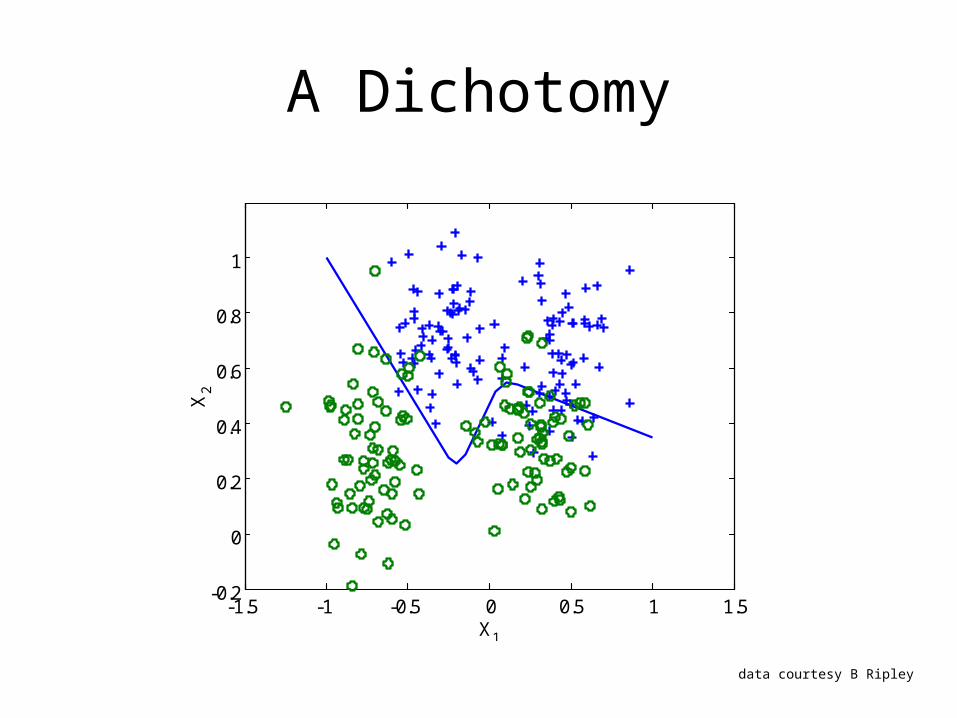
A Dichotomy
-1.5 -1 -0.5 0 0.5 1 1.5-0.2
0
0.2
0.4
0.6
0.8
1
X1
X2
data courtesy B Ripley
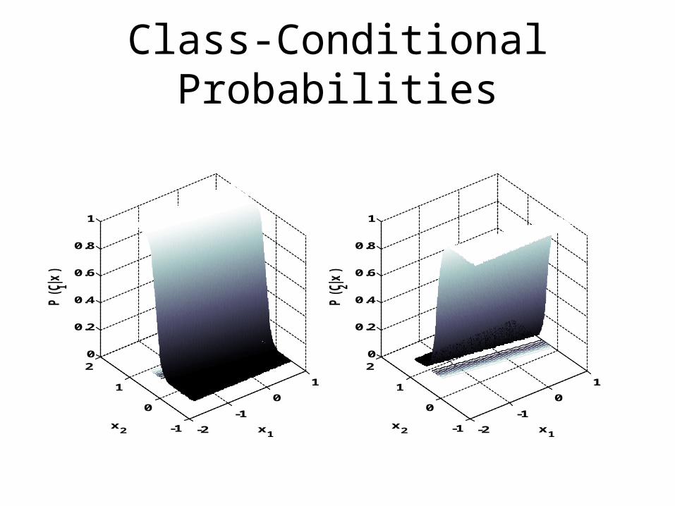
Class-Conditional Probabilities
-2
-1
0
1
-1
0
1
20
0.2
0.4
0.6
0.8
1
x1
x2
P(C1|x
)
-2
-1
0
1
-1
0
1
20
0.2
0.4
0.6
0.8
1
x1
x2
P(C2|x
)
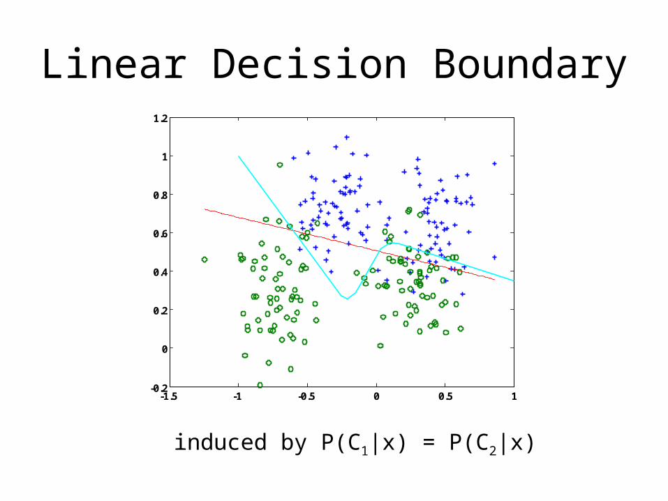
Linear Decision Boundary
induced by P(C1|x) = P(C2|x)
-1.5 -1 -0.5 0 0.5 1-0.2
0
0.2
0.4
0.6
0.8
1
1.2
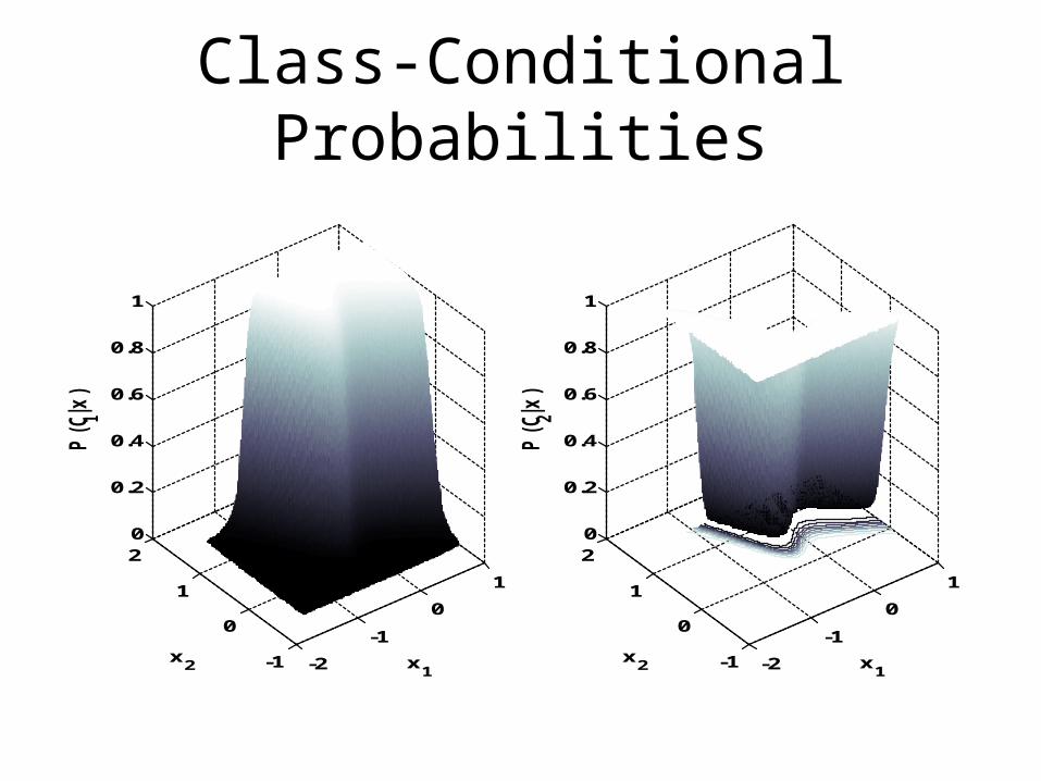
Class-Conditional Probabilities
-2
-1
0
1
-1
0
1
20
0.2
0.4
0.6
0.8
1
x1
x2
P(C
1|x)
-2
-1
0
1
-1
0
1
20
0.2
0.4
0.6
0.8
1
x1
x2
P(C
2|x)
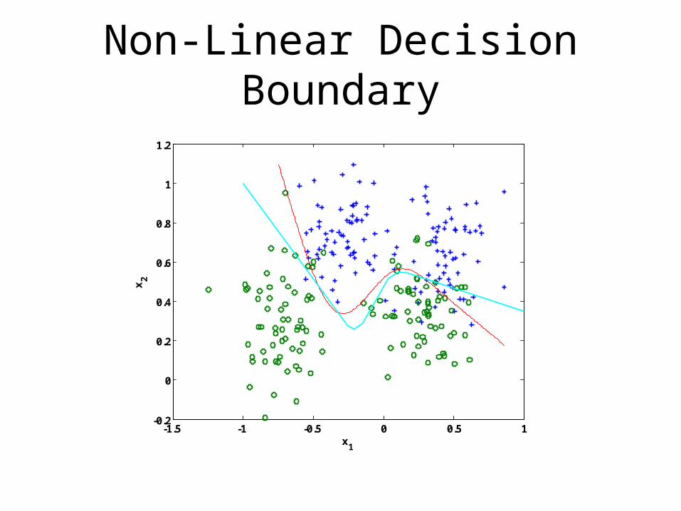
Non-Linear Decision Boundary
-1.5 -1 -0.5 0 0.5 1-0.2
0
0.2
0.4
0.6
0.8
1
1.2
x1
x2
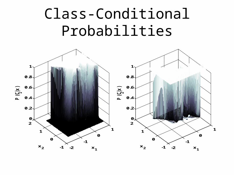
Class-Conditional Probabilities
-2
-1
0
1
-1
0
1
20
0.2
0.4
0.6
0.8
1
x1
x2
P(C
1|x)
-2
-1
0
1
-1
0
1
20
0.2
0.4
0.6
0.8
1
x1
x2
P(C
2|x)
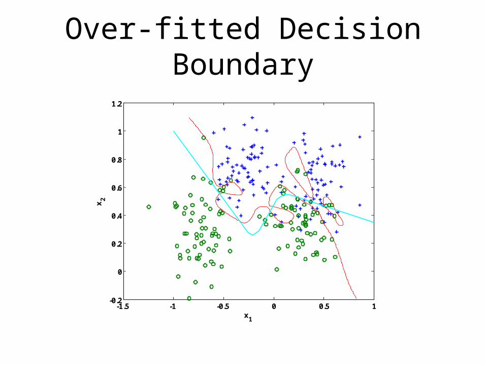
Over-fitted Decision Boundary
-1.5 -1 -0.5 0 0.5 1-0.2
0
0.2
0.4
0.6
0.8
1
1.2
x1
x2
Invariances
• e.g. scale, rotation, translation
• augment training data
• design regularizer– tangent propagation (Simmard et al, 1992)
• build into MLP structure– convolutional networks (LeCun et al, 1989)
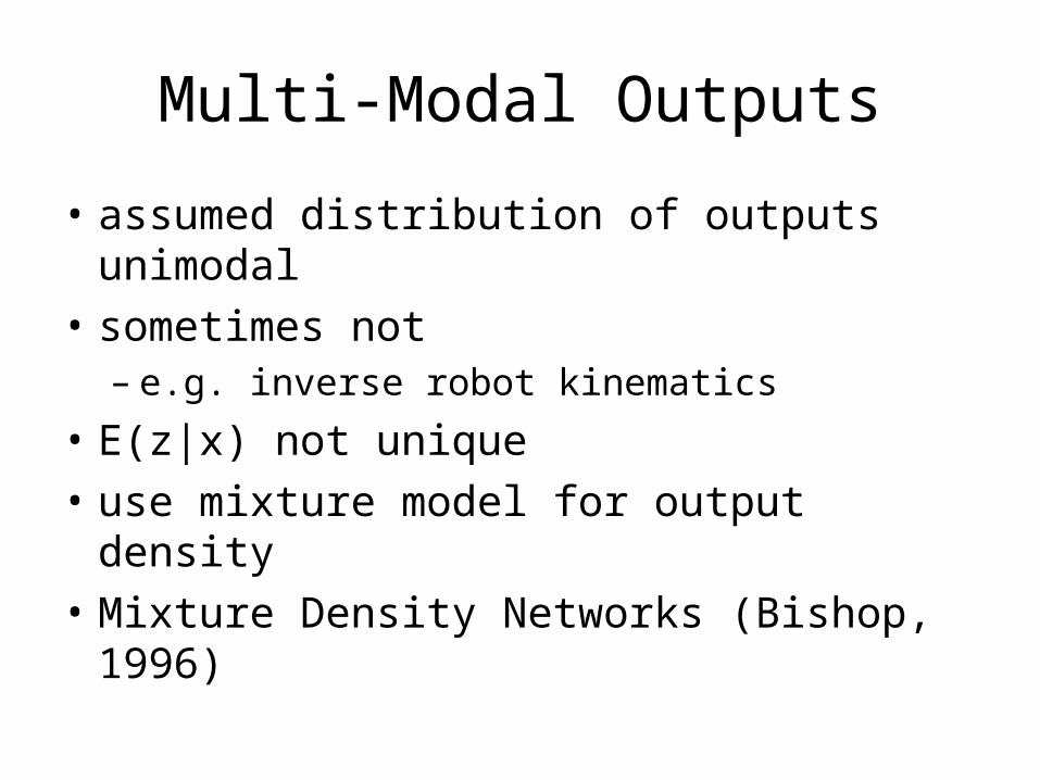
Multi-Modal Outputs
• assumed distribution of outputs unimodal
• sometimes not– e.g. inverse robot kinematics
• E(z|x) not unique
• use mixture model for output density
• Mixture Density Networks (Bishop, 1996)
Bayesian MLPs
• deterministic treatment
• point estimates, E(z|x)
• can use MLP as estimator in a Bayesian treatment– non-linearity → approximate solutions
• approximate estimate of spread
E((z-y)2|x)
NETTalk
• Introduced by T Sejnowski & C Rosenberg
• First realistic ANNs demo
• English text-to-speech non-phonetic
• Context sensitive– brave, gave, save, have (within word)– read, read (within sentence)
• Mimicked DECTalk (rule-based)
Representing Text
• 29 “letters” (a–z + space, comma, stop)– 29 binary inputs indicating letter
• Context– local (within word) – global (sentence)
• 7 letters at a time: middle → AFs– 3 each side give context, e.g. boundaries
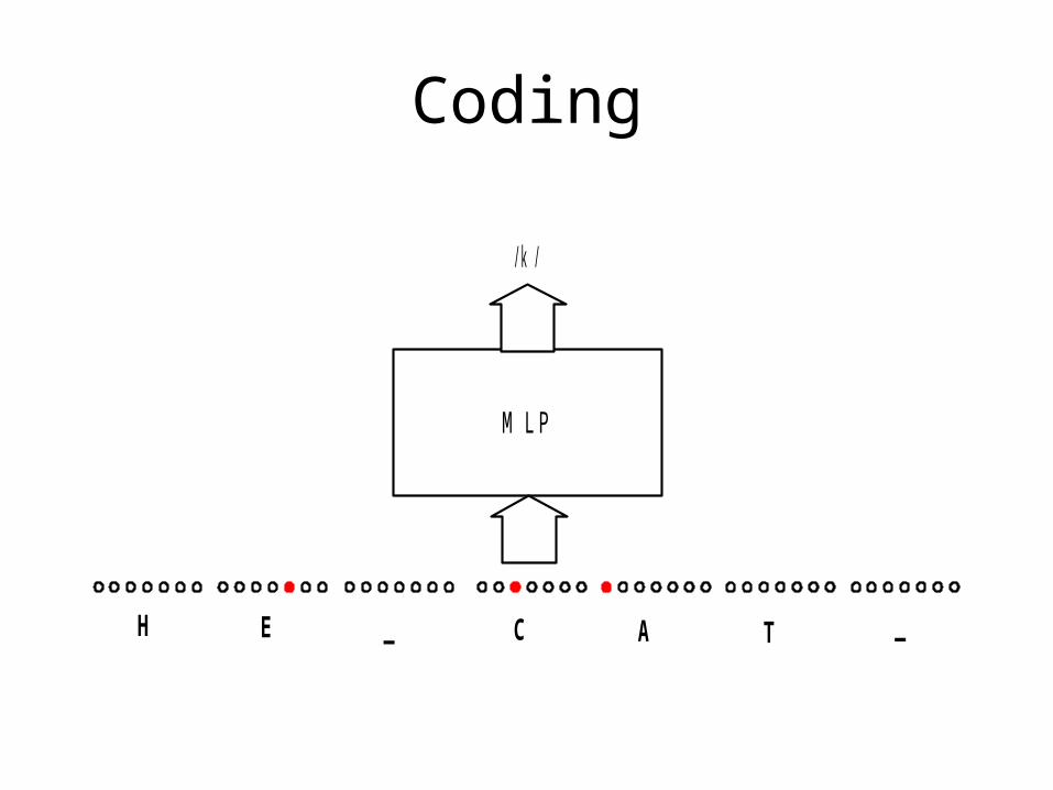
Coding
MLP
H E _ C A T _
/k /
Wave Sound
NETTalk Performance
• 1024 words continuous, informal speech
• 1000 most common words
• Best performing MLP• 26 o/p, 7x29 i/p, 80
hidden• 309 units, 18,320 weights• 94% training accuracy• 85% testing accuracy