Embed Size (px)
Citation preview
THE MYTH OF LONG-HORIZON PREDICTABILITY
Jacob Boudoukh,a Matthew Richardsonb and Robert F. Whitelawb*
This Version: November 14, 2005
* a Arison School of Business, IDC and NBER; b Stern School of Business, New York University and NBER. We would like to thank Jeff Wurgler, John Cochrane (the discussant), and seminar participants at Yale University, New York University and the NBER asset pricing program for helpful comments. Contact: Prof. M. Richardson, NYU, Stern School of Business, 44 W. 4th St., New York, NY 10012; [email protected].
THE MYTH OF LONG-HORIZON PREDICTABILITY
Abstract
The prevailing view in finance is that the evidence for long-horizon stock return predictability
is significantly stronger than that for short horizons. We show that for persistent regressors, a
characteristic of most of the predictive variables used in the literature, the estimators are
almost perfectly correlated across horizons under the null hypothesis of no predictability. For
example, for the persistence levels of dividend yields, the analytical correlation is 99%
between the 1- and 2-year horizon estimators and 94% between the 1- and 5-year horizons, due
to the combined effects of overlapping returns and the persistence of the predictive variable.
Common sampling error across equations leads to ordinary least squares coefficient estimates
and R2s that are roughly proportional to the horizon under the null hypothesis. This is the
precise pattern found in the data. The asymptotic theory is corroborated, and the analysis
extended by extensive simulation evidence. We perform joint tests across horizons for a
variety of explanatory variables, and provide an alternative view of the existing evidence.
1
I. Introduction
Over the last two decades, the finance literature has produced growing evidence of stock return
predictability, though not without substantive debate. The strongest evidence cited so far
comes from long-horizon stock returns regressed on variables such as dividend yields, term
structure slopes, and credit spreads, among others. A typical view is expressed in Campbell,
Lo, and MacKinlay’s standard textbook for empirical financial economics, The Econometrics
of Financial Markets (1997, p.268):
At a horizon of one month, the regression results are rather unimpressive: The
R2 statistics never exceed 2%, and the t-statistics exceed 2 only in the post-
World War II subsample. The striking fact about the table is how much
stronger the results become when one increases the horizon. At a two-year
horizon the R2 statistic is 14% for the full sample … at a four-year horizon the
R2 statistic is 26% for the full sample.
However, there is an alternative interpretation of this evidence: Researchers should be
equally impressed by the short- and long-horizon evidence for the simple reason that the
regressions are almost perfectly correlated. For an autocorrelation of 0.953 for annual dividend
yields, we show analytically that the 1-year and 2-year predictive estimators are 98.8%
correlated under the null hypothesis of no predictability. For longer horizons, the correlations
are even higher, reaching 99.6% between the 4- and 5-year horizon estimators. This degree of
correlation manifests itself in multiple-horizon regressions in a particularly unfortunate way.
2
Since the sampling error that is almost surely present in small samples shows up in each
regression, both the estimator and R2 are proportional to the horizon.
This paper provides analytical expressions for the correlations across multiple-horizon
estimators, and then shows, through simulations, that these expressions are relevant in small
samples. The analytical expressions relate the correlations across these estimators to both the
degree of overlap across the horizons and the level of persistence of the predictive variable.
Our findings relate to an earlier literature looking at joint tests of the random walk hypothesis
for stock prices using multiple-horizon variance ratios and autocorrelations, among other
estimators (see, e.g., Richardson and Smith (1991, 1994) and Richardson (1993)). This earlier
literature stresses accounting for the degree of overlap. The problem here is much more severe.
In the univariate framework, the predictive variable—past stock returns—is approximately
independently and identically distributed (IID). In this paper’s framework, the predictive
variable, e.g., dividend yields, is highly persistent.
Our simulations show that any sampling error in the data under the null hypothesis of no
predictability appears in the same manner in every multiple-horizon regression when the
predictive variable is highly persistent. Using box plots and tables describing the relation
across the multiple horizon estimates and R2s, we show the exact pattern one should expect
under the null hypothesis: The multiple-horizon estimates are monotonic in the horizon
approximately two-thirds of the time, and the mean ratios of the 2- to 5-year estimators to the
1-year estimator are 1.93, 2.80, 3.59, and 4.32, respectively. Consider the actual estimated
coefficients for the regression of 1- to 5-year stock returns on dividend yields over the 1926–
2004 sample period: 0.131, 0.257, 0.390, 0.461, and 0.521. These correspond to monotonically
increasing estimates with corresponding ratios of 1.96, 2.98, 3.53, and 3.99. We show that

3
these estimates lie in the middle of the distribution of possible outcomes under the null
hypothesis.
The theoretical and simulation analyses stress the importance of interpreting the evidence
jointly across horizons. We develop an analytical expression for a joint test based on the Wald
statistic. While a high level of persistence means that it can be dangerous to interpret
regressions over multiple horizons, the joint tests show that this persistence may lead to
powerful tests for economies in which predictability exists. Such predictability may take a
particular form, in which the multiple-horizon coefficients are much less tied together than the
null hypothesis implies. Applying the joint tests to commonly used predictive variables, we
point out various anomalies and contrast our results with the conclusions of the existing
literature.
Among the standard set of variables, none generate joint test statistics that are significant at
the 10% level under the simulated distribution. Interestingly, the only variable that is
significant at the 10% level under the asymptotic distribution is the risk-free rate, despite the
fact that the associated horizon-by-horizon p-values are larger and the R2s are smaller than for
many of the other variables, including the dividend yield and the book-to-market ratio. Among
more recently developed variables, joint tests confirm the ability of both the net payout yield
(Boudoukh, Michaely, Richardson, and Roberts (2005)) and the equity share of new issuances
(Baker and Wurgler (2000)) to forecast stock returns across all horizons.
The paper proceeds as follows. In Section 2, we provide the expressions for analyzing
multiple-horizon regressions and show that the basic findings carry through to small samples.
The small sample results are especially alarming in the context of the existing literature.

4
Section 3 applies the results to a number of data series and evaluates existing evidence using
joint tests of predictability. Section 4 concludes.
II. Multiple Horizon Regressions
A. The Existing Literature
Fama and French (1988) is the first paper to document evidence of multivariate stock return
predictability over multiple horizons.1 In brief, they regress overlapping stock returns of one
month to four years on dividend yields, reporting coefficients and R2s that increase somewhat
proportionately with the horizon. As it documents what has become one of the dominant
stylized facts in empirical finance, the paper has over 250 citations to date. To illustrate the
consensus view, consider part of John Cochrane’s description of the three most important facts
in finance in his survey, “New Facts in Finance” (1999, p.37).
Now, we know that …
[Fact] 2. Returns are predictable. In particular: Variables including the
dividend/price (d/p) ratio and term premium can predict substantial amounts
of stock return variation. This phenomenon occurs over business cycle and
longer horizons. Daily, weekly, and monthly stock returns are still close to
unpredictable…
This fact is emphasized repeatedly in other surveys (see, e.g., Fama (1998, p.1578),
Campbell (2000, p.1522 and 2003, p.5) and Barberis and Thaler (2003, p.21), among others),
1 See also Campbell and Shiller (1988).
5
is often used to calibrate theoretical models (see, among others, Campbell and Cochrane
(1999, p.206), Campbell and Viceira (1999, p.434), Barberis (2000, p.225), Menzly, Santos,
and Veronesi (2004, p.2), and Lettau and Ludvigson (2005, p.584)), and in motivation for new
empirical tests (e.g., Ferson & Korajczyk (1995, p.309), Patelis (1997, p.1951), Lettau &
Ludvigson (2001, p.815), and Ait-Sahalia and Brandt (2001, p.1297)).
It is fairly well known since Fama and French (1988), and in particular from Campbell
(2001), that the key determinants of long-horizon predictability are
(i) The extent of predictability at short horizons, and
(ii) The persistence of the regressor.
The R2s at long horizons relative to a single-period R2 are a function of (ii). Holding
everything else constant—single-period predictability in particular—higher persistence results
in a higher fraction of explainable long-horizon returns. As a function of the horizon, the R2
first rises with the horizon, but eventually decays, due to the exponential decline in the
informativeness of the predictive variable. As we show below, (ii) also matters in the case of
no predictability, but in the presence of sampling error. Nevertheless, this important fact has
not been used as the main line of attack against evidence supporting the multivariate
predictability of stock returns.
Three principal alternative lines of criticism have been put forward in the literature. The
first involves data snooping, which is perhaps best described by Foster, Smith, and Whaley
(1997). The idea is that the levels of predictability found at short horizons are not surprising,
given the number of variables from which researchers can choose. A variety of papers support
these findings somewhat, including Bossaerts and Hillion (1999), Cremers (2002), and Goyal
and Welch (2003).
6
A second approach looks at the small sample biases of the estimators. Stambaugh (1999)
shows that the bias can be quite severe, given the negative correlation between
contemporaneous shocks to returns and the predictive variable, which usually involves some
type of stock price deflator. His findings suggest much less predictability once the estimators
are adjusted for this bias. However, Lewellen (2004) argues that the effect of the bias may be
much smaller if one takes the persistence of the predictive variable into account. Lewellen’s
approach is similar to Stambaugh’s (1999) Bayesian analysis of the predictability problem.
While both of these papers certainly question the magnitude of the predictability, they do not
address long-horizon predictability per se.
The third line of criticism, first explored by Richardson and Stock (1989) in a univariate
setting, uses an alternative asymptotic theory, in which the horizon increases with the sample
size. Valkanov (2003) argues that long-horizon regressions have poor properties relative to
standard asymptotics.2 He shows that the estimators may no longer be consistent, and have
limiting distributions that are functionals of Brownian motions; in fact, the distributions are
not normal, and are not centered on the true coefficient. Valkanov then shows that this
alternative asymptotic theory works better in small samples. His results can be viewed as the
theoretical foundation for earlier simulated distributions by Kim and Nelson (1993) and
Goetzmann and Jorion (1993), and for the intuition put forward by Kirby (1997), who uses
standard asymptotics.
Aside from these three methodology-based lines of criticism of the stock return
predictability literature, there is scant evidence of empirical-based critique of long horizon
predictability, one recent exception being Ang and Bekaert (2005). Our paper focuses on a
7
different methodological aspect of predictability, examining the joint properties of the
regression estimators across horizons. The conclusions here closely resemble those of
Richardson and Smith (1991) and Richardson (1993) regarding long-horizon evidence against
the random walk in Fama and French (1998) and Poterba and Summers (1988). In many ways,
the arguments here are more damaging, because we show that the degree of correlation across
the multiple-horizon estimators is much higher than it is in the case of long-horizon tests for
the random walk. In fact, the null hypothesis of no predictability implies the exact pattern in
coefficients and R2s found in papers presenting evidence in favor of predictability. We show
these results in the next two subsections.
B. Multiple Horizon Regressions: Statistical Properties
We consider regression systems of the following type:
,,,
,,
1,111,
KtttKKKtt
JtttJJJtt
ttttt
XR
XR
XR
++
++
++
++=
++=
++=
εβα
εβα
εβα
M
M
(1)
where JttR +, is the J-period stock return, tX is the predictor, e.g., the dividend yield, and Jtt +,ε
is the error term over J periods. As is well known from Hansen and Hodrick (1980) and
Hansen (1982), among others, the error terms are serially correlated due to overlapping
observations. Using the standard generalized method of moments calculations under the null
hypothesis of no predictability and under conditional homoskedasticity (e.g., Richardson and
2 Ang and Bekeart (2005) show that the statistical significance of long horizon regressions is overstated once the researcher adjusts for heteroskedasticity and the overlapping errors by imposing the null in estimation.
8
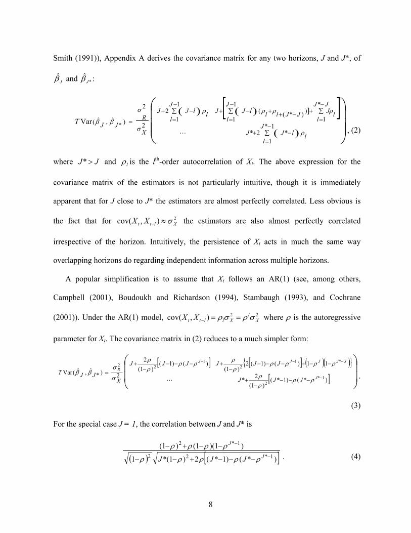
Smith (1991)), Appendix A derives the covariance matrix for any two horizons, J and J*, of
Jβ̂ and *ˆ
Jβ :
( ) ( )[ ]( )
∑−
=−+
∑−
=+−++∑
−
=−+∑
−
=−+
=1*
1*2*
*
1))*(
1
1(
1
12
2
2
)*ˆ,ˆ(
]Var
J
lllJJ
JJ
llJJJl
J
lllJJ
J
lllJJ
X
RJJT
ρ
ρρρρ
σ
σ
ββ
L , (2)
where JJ >* and lρ is the lth-order autocorrelation of Xt. The above expression for the
covariance matrix of the estimators is not particularly intuitive, though it is immediately
apparent that for J close to J* the estimators are almost perfectly correlated. Less obvious is
the fact that for 2),cov( Xltt XX σ≈− the estimators are also almost perfectly correlated
irrespective of the horizon. Intuitively, the persistence of Xt acts in much the same way
overlapping horizons do regarding independent information across multiple horizons.
A popular simplification is to assume that Xt follows an AR(1) (see, among others,
Campbell (2001), Boudoukh and Richardson (1994), Stambaugh (1993), and Cochrane
(2001)). Under the AR(1) model, 22),cov( Xl
Xlltt XX σρσρ ==− where ρ is the autoregressive
parameter for Xt. The covariance matrix in (2) reduces to a much simpler form:
[ ] [ ]{ ( )( )}[ ]
−
−−−
−−−−
+
−−+−−−−
+−−−−
+=
)*()1*()1(
2*
11)()1(2)1(
)()1()1(
2
2)*ˆ,ˆ(Var
1*2
*12
122
J
JJJJJ
R
JJJ
JJJJJJ
XJJT
ρρρρ
ρρρρρρρρ
ρρ
σ
σββ
L.
(3)
For the special case J = 1, the correlation between J and J* is
( ) [ ])*()1*(2)1(*1
)1)(1()1(1*22
1*2
−
−
−−−+−−
−−+−J
J
JJJ ρρρρρ
ρρρρ. (4)
9
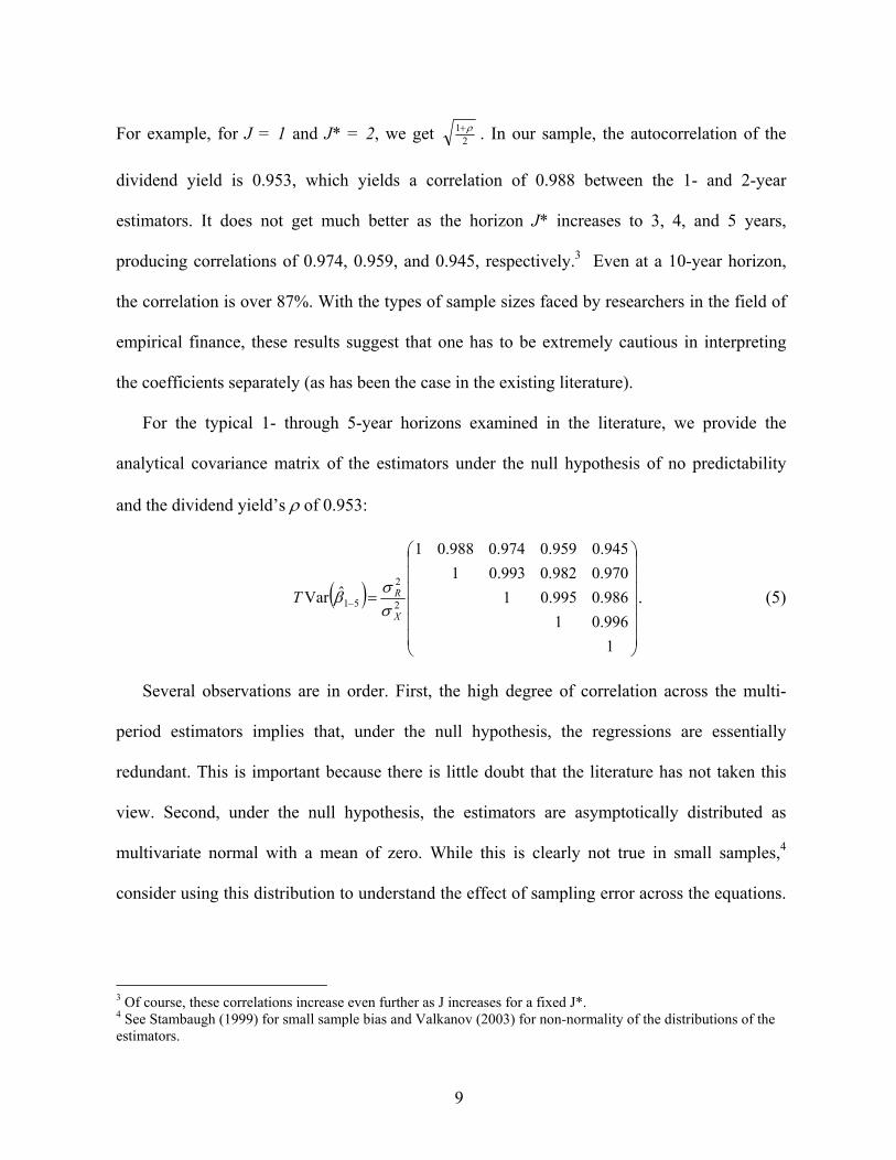
For example, for J = 1 and J* = 2, we get 21 ρ+ . In our sample, the autocorrelation of the
dividend yield is 0.953, which yields a correlation of 0.988 between the 1- and 2-year
estimators. It does not get much better as the horizon J* increases to 3, 4, and 5 years,
producing correlations of 0.974, 0.959, and 0.945, respectively.3 Even at a 10-year horizon,
the correlation is over 87%. With the types of sample sizes faced by researchers in the field of
empirical finance, these results suggest that one has to be extremely cautious in interpreting
the coefficients separately (as has been the case in the existing literature).
For the typical 1- through 5-year horizons examined in the literature, we provide the
analytical covariance matrix of the estimators under the null hypothesis of no predictability
and the dividend yield’s ρ of 0.953:
( )
=−
1996.01986.0995.01970.0982.0993.01945.0959.0974.0988.01
ˆVar 2
2
51X
RTσσβ . (5)
Several observations are in order. First, the high degree of correlation across the multi-
period estimators implies that, under the null hypothesis, the regressions are essentially
redundant. This is important because there is little doubt that the literature has not taken this
view. Second, under the null hypothesis, the estimators are asymptotically distributed as
multivariate normal with a mean of zero. While this is clearly not true in small samples,4
consider using this distribution to understand the effect of sampling error across the equations.
3 Of course, these correlations increase even further as J increases for a fixed J*. 4 See Stambaugh (1999) for small sample bias and Valkanov (2003) for non-normality of the distributions of the estimators.
10
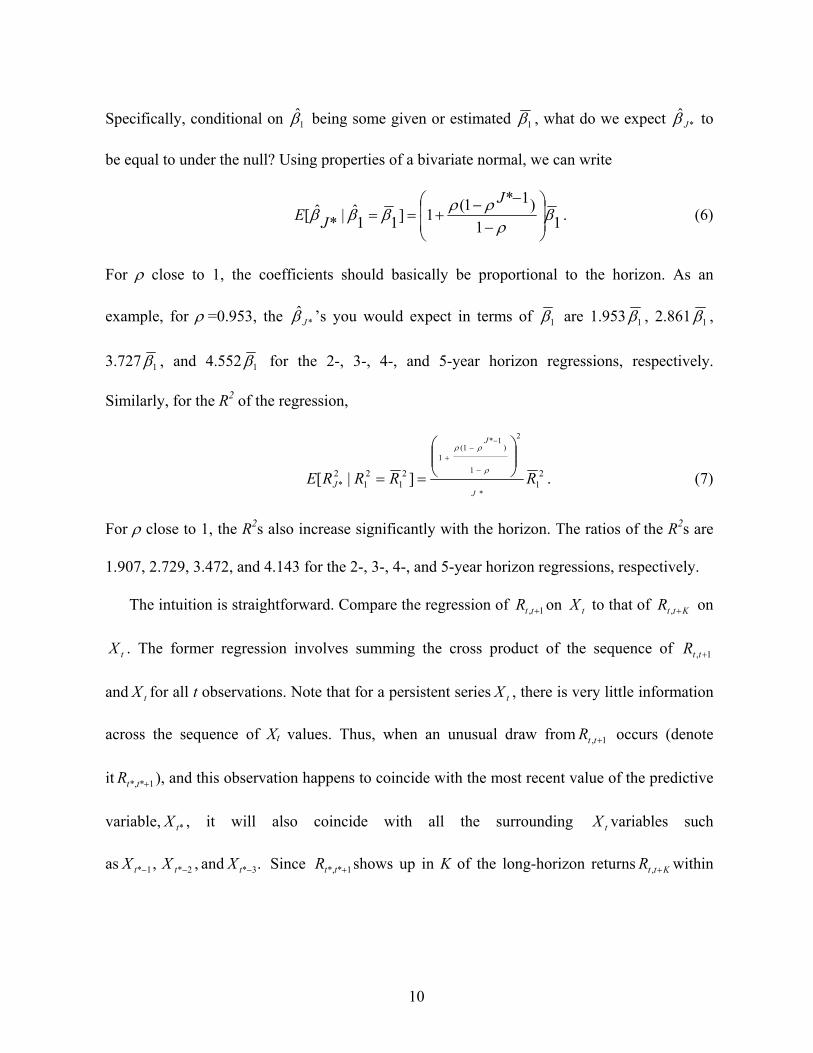
Specifically, conditional on 1̂β being some given or estimated 1β , what do we expect *ˆ
Jβ to
be equal to under the null? Using properties of a bivariate normal, we can write
11)1*1(1]11
ˆ|*ˆ[ β
ρρρβββ
−
−−+==
JJE . (6)
For ρ close to 1, the coefficients should basically be proportional to the horizon. As an
example, for ρ =0.953, the *ˆ
Jβ ’s you would expect in terms of 1β are 1.953 1β , 2.861 1β ,
3.727 1β , and 4.552 1β for the 2-, 3-, 4-, and 5-year horizon regressions, respectively.
Similarly, for the R2 of the regression,
21
21
21
2*
*
2
1
)1*
1(1
]|[ RRRREJ
J
J
==−
−−
+
ρ
ρρ
. (7)
For ρ close to 1, the R2s also increase significantly with the horizon. The ratios of the R2s are
1.907, 2.729, 3.472, and 4.143 for the 2-, 3-, 4-, and 5-year horizon regressions, respectively.
The intuition is straightforward. Compare the regression of 1, +ttR on tX to that of KttR +, on
tX . The former regression involves summing the cross product of the sequence of 1, +ttR
and tX for all t observations. Note that for a persistent series tX , there is very little information
across the sequence of Xt values. Thus, when an unusual draw from 1, +ttR occurs (denote
it 1**, +ttR ), and this observation happens to coincide with the most recent value of the predictive
variable, *tX , it will also coincide with all the surrounding tX variables such
as ,1*−tX ,2*−tX and .3*−tX Since 1**, +ttR shows up in K of the long-horizon returns KttR +, within
11
the sample period (i.e., in 1*,1* +−+ tKtR , 2*,2* +−+ tKtR ,…, KttR +**, ), the impact of the unusual draw will
be roughly K times larger in the long-horizon regression than in the one-period regression.
C. Multiple Horizon Regressions: Joint Tests
At first glance, the results in Section II.B provide a fairly devastating critique of the strategy of
running multiple long-horizon regressions. However, this view is not necessarily accurate.
Because the regressions are linked so closely under the null hypothesis, joint tests may have
considerable power under alternative models.
What are these alternatives? The models must be such that the long horizons pick up
information not contained in short horizons. The standard model, in which short-horizon
returns are linear in the current predictor and that predictor follows a persistent ARMA
process, is clearly not a good candidate. It would be better to focus on estimating the short-
horizon and the ARMA process directly in this case (see, e.g., Campbell (2001), Hodrick
(1992), and Boudoukh and Richardson (1994), among others). It should be noted, though, that
the standard model is often chosen for reasons of parsimony rather than on an underlying
theoretical basis.
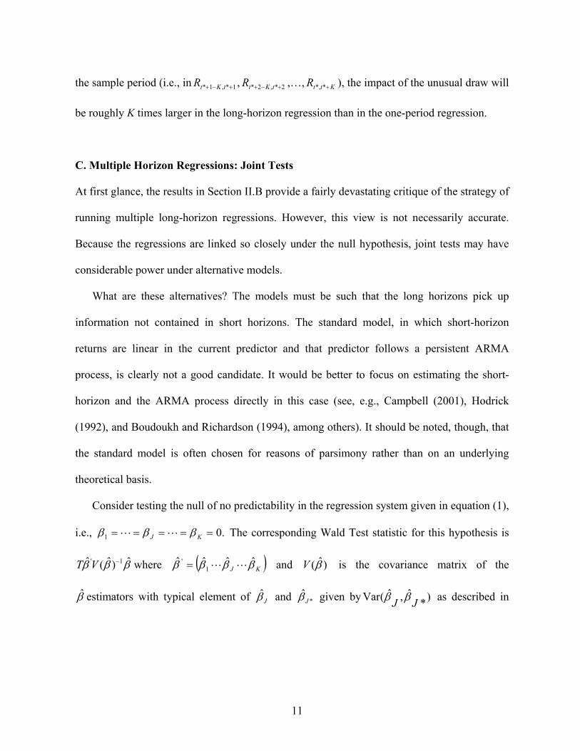
Consider testing the null of no predictability in the regression system given in equation (1),
i.e., .01 ===== KJ βββ LL The corresponding Wald Test statistic for this hypothesis is
βββ ˆ)ˆ(ˆ 1' −VT where ( )KJ ββββ ˆˆˆˆ1
' LL= and )ˆ(βV is the covariance matrix of the
β̂ estimators with typical element of Jβ̂ and *ˆ
Jβ given by )*ˆ,ˆ(Var JJ ββ as described in
12
equation (2).5 The statistic follows an asymptotic chi-squared distribution with degrees of
freedom given by the number of horizons used in estimation. Note that )ˆ(βV is a function of
the autocorrelation structure of the Xt variable (i.e., its persistence) as well as the degree of
overlap between horizons, i.e., J versus J*. Aside from the magnitude of the β̂ estimators,
what matters is whether the pattern in β̂ across horizons is consistent with the correlation
implied by )ˆ(βV .
To see this, consider performing a Wald Test of the hypothesis .021 == ββ The
corresponding Wald statistic is given by
( )
−
−+ +
ρβββ
σσ ρ
β
122 211
222
12
2
R
XT . (8)
For a given sample size T and estimated coefficient 11ˆ ββ = , this statistic is minimized at
12 )1(ˆ βρβ += . Since a low value of the statistic implies less evidence against the null, this
result means that we not only expect a nonzero 2β̂ under the null but that it should be of a
magnitude greater than the 1β̂ estimate. In fact, for a highly persistent regressor, the Wald
statistic is minimized when the 2-period coefficient is almost double the one-period
coefficient. Of course, the denominator of the test statistic goes to zero as the autocorrelation
approaches one, so even small deviations from the predicted pattern under the null may
generate rejections if the regressor is sufficiently persistent.
These results provide important clues in searching for powerful tests against the null of no
predictability. If the alternative hypothesis does not imply coefficient estimates that increase at
5 For other examples of joint tests in the predictability framework, see, for example, Richardson and Smith

13
the same rate across horizons or that are not as heavily tied to the predictive variable’s
persistence, one can find evidence of predictability even with modestly sized coefficients. But
the fact that the no predictability null and the standard ARMA predictive model imply similar
coefficient patterns (and thus low power) does not mean the null is false.
Treating the individual coefficient estimates separately in a joint setting can lead to very
misleading conclusions. The null hypothesis of no predictability as described by the Wald Test
is most supported in the data when we observe monotonically increasing/decreasing
coefficient estimates that can be described by the horizon and persistence of the predictive
variable. This is the exact pattern documented in the original Fama and French (1988) and
Campbell and Shiller (1988) papers. One wonders how the finance literature would have
treated these papers if armed with this fact, especially given the weak evidence of
predictability at short horizons and also in the context of the previously mentioned data
snooping arguments (e.g., Foster, Smith, and Whaley (1997)) and small sample bias
(Stambaugh (1999)), both of which suggest that short-horizon significance is overstated.
D. Multiple Horizon Regressions: Simulation Evidence
The theoretical results in Sections II.B and II.C are based on asymptotic properties of fixed-
horizon estimators. A priori there is reason to be wary of these results in small samples,
particularly because of the considerable evidence of a bias in the coefficient estimators and of
non-normality as discussed in Section II.A. Therefore, it is useful to evaluate the small sample
properties of the estimators in general, and the patterns in sampling error across equations in
(1991), Hodrick (1992) and Ang and Bekeart (2005), among others.
14
particular. Previewing the results to come, the basic tenet of equations (2) and (3), namely, the
dependence across equations, carries through to small samples.
We simulate the model in equation (1) under the assumption of no predictability, an AR(1)
process on tX , and 75 years of annual data. The analysis is performed over 1- to 5-year
horizons with the AR parameter ρ, the standard deviation of tX and εt,t +1, and the correlation
between εt,t +1 and ut,t +1 ≡ Xt +1 − ρXt( ) chosen to match the data.6 The simulations involve
100,000 replications each.
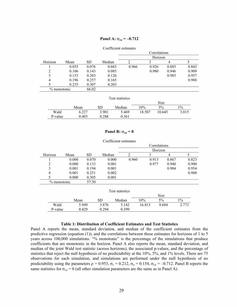
Table 1A reports the simulated correlation matrix of the multiple-horizon estimators.
Consistent with the theoretical analytical calculations in Section II.B, the correlations tend to
be high, even for the most distant horizons. The simulated correlations between the 1-year and
2- to 5-year horizon estimators are 0.966, 0.926, 0.885, and 0.843, respectively, showing that
the correlation calculations under the fixed-horizon asymptotics hold in small samples. Thus,
the estimators’ almost perfect cross-correlation leads to little independent information across
equations, and the sampling error that is surely present in small samples shows up in every
equation in (1).
As shown in Section II.B, persistence (i.e., ρ) is an important determinant of the magnitude
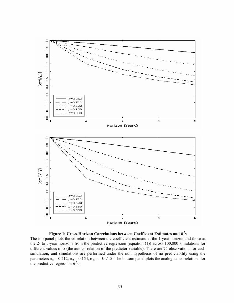
of the correlation matrix of the multiple-horizon estimators. Figure 1A graphs the correlation
between the 1-year and 2- to 5-year horizon estimators for values ρ = 0.953, 0.750, 0.500,
0.250, and 0.000. Consistent with the asymptotic theory, the correlations decrease as ρ falls.
The drop-off can be quite large as the horizon increases. As a function of the above ρ values,
6 Specifically, for the regression of annual stock returns on the most commonly used predictive variable, namely, dividend yields, we estimate .712.0 and 154.0 0.202,= ,953.0 −=== uu εσσεσρ While the magnitudes of
15
the 1- and 2-year estimators have correlations of 0.966, 0.917, 0.849, 0.776, and 0.698,
respectively, and the 1- and 5-year estimators have correlations of 0.843, 0.684, 0.544, 0.465,
and 0.429. Even when the predictive variable has no persistence, the correlation can still be
quite high due to the overlapping information across the multiple-horizon returns.
However, the staggering result in Table 1A is that 66% of all the replications produce
estimates that are monotonic in the horizon. That is, almost two-thirds of the time, the data
produce coefficients increasing or decreasing with the horizon, coinciding with the predictions
from the asymptotic theory. To understand how unlikely monotonicity is, suppose that the five
different multiple-horizon estimators were IID. In this setting, the probability of a monotonic
relation is 0.83%, approximately 1/78th of the true probability for the multiple-horizon
estimators. Even with overlapping horizons, monotonicity drops sharply as ρ falls, i.e., from
66% to 37%, 20%, 11%, and 6% for ρ = 0.750, 0.500, 0.250, and 0.000, respectively. This
result further highlights the importance of persistence in the predictive variable for generating
these patterns.
One possible explanation for this finding is that the small sample bias increases with the
horizon (e.g., Stambaugh (1999), Goetzmann and Jorion (1993), and Kim and Nelson (1993)).
Table 1A confirms that the small sample bias increases with the horizon, with the means of the
1- to 5-year coefficients equal to 0.055, 0.106, 0.153, 0.196, and 0.235, respectively. To
investigate whether the monotonicity is due to this bias, Table 1B duplicates Table 1A under
the assumption that σεu = 0. For this value, the small sample bias is theoretically zero, and the
estimates are unbiased in our simulations. Interestingly, the monotonicity falls only slightly, to
σ u and σε do not matter, this is not true for either the persistence variable ρ (Boudoukh and Richardson (1994)) or the correlation σεu (e.g., Stambaugh (1999)). Thus, we also investigate different values for these parameters.
16
57%. Furthermore, Table 1B shows that the correlation matrix across the multiple-horizon
estimators is virtually identical to that in Table 1A. Thus, the monotonicity is driven by the
almost perfect correlation across the estimators and the increasing horizon, not by the small
sample bias.
As described in Section II.A, much of the literature has argued for predictability by
focusing on the increase in the coefficient estimates as a function of the horizon. Both
theoretically and in simulation, we show that this result is expected under the null hypothesis
of no predictability. An alternative measure of predictability also considered in the literature is
the magnitude and pattern of R2s across horizons. While the R2 is linked directly to the
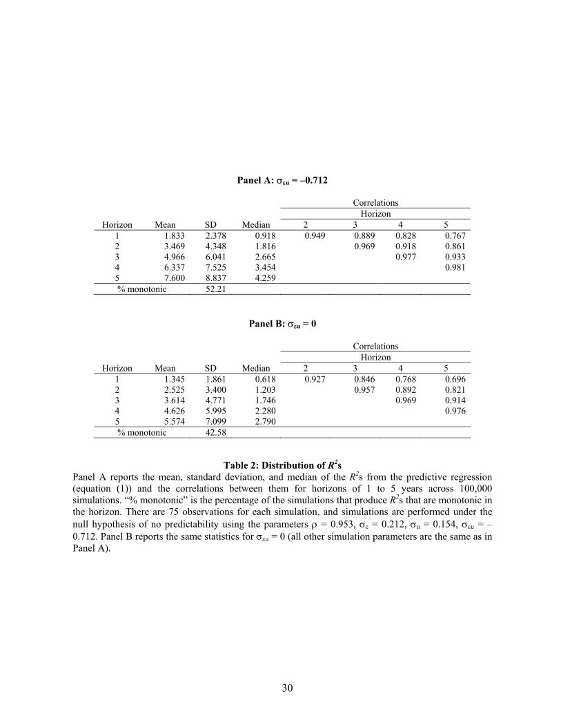
coefficient estimate, it is nonetheless a different statistic of the data. Table 2A reports the
simulated correlation matrix of the multiple-horizon R2s as well as their means, medians,
standard deviations, and monotonicity properties.
Similar to Table 1A, the R2s are all highly correlated across horizons. For example, the
simulated correlations between the 1-year and 2- to 5-year horizon R2s are 0.949, 0.889, 0.828,
and 0.767, respectively. This degree of correlation leads to R2s that are monotonic in the
horizon 52% of the time under the null hypothesis—the exact pattern documented in the
literature. This result is not due to the Stambaugh (1999) small sample bias, as both the degree
of correlation and monotonicity also appear in the simulated data without the bias (see Table
2B, where the cross-equation correlation is zero). Also, analogous to the evidence for the
multiple-horizon coefficient estimators, the degree of cross-correlation and monotonicity
depends crucially on the level of persistence ρ of the predictive variable.
Figures 1A and 1B show the correlation coefficients between the 1- and the J-period β
estimates and R2s. The correlations are plotted for different persistence parameters, and the
17
figures illustrate both the monotonicity and near linearity one would expect and the
dependence of this effect on the persistence parameter.
The theoretical calculations of Section II.B imply an even stronger condition than
monotonicity. For ρ close to 1, the coefficients and R2s should increase one-for-one with the
horizon under the null hypothesis. Because this is the typical pattern found in US data, it
seems worthwhile to investigate this implication through a simulation under the null
hypothesis of no predictability. We compare the ratio of the 2- to 5-year coefficient and R2
estimates to the 1-year estimates. Since there are numerical issues when using denominators
close to zero, we run the analysis under the condition that the 1-year estimate have an absolute
value greater than 0.01, or an R2 greater than 0.5%. Approximately 88% and 62% of the
simulations respectively satisfy these criteria.
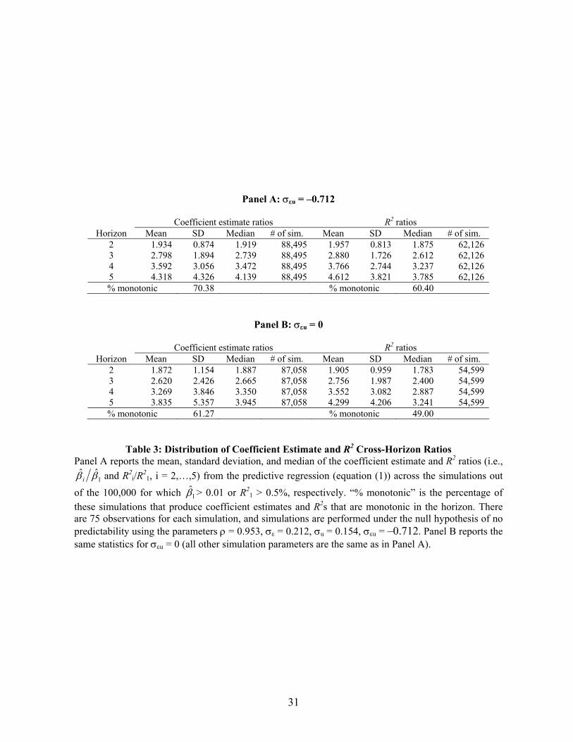
Table 3A contains the results. As predicted by the theory, the mean ratios of the estimates
are 1.93, 2.80, 3.59, and 4.32 for the 2-, 3-, 4-, and 5-year horizons, respectively. The R2s are
equally dramatic, with corresponding ratios of 1.96, 2.88, 3.77, and 4.61.7 Note that these
simulations are performed under the null hypothesis of no predictability. The βs are zero, but
the other parameters are calibrated to match the joint distribution of stock returns and dividend
yields in the data. How do these results compare with the estimated coefficients and R2s from
the actual data? In the data, the ratios for the 2-, 3-, 4-, and 5-year horizons are 1.96, 2.98,
3.53, and 3.99 for the β estimates, and 1.85, 3.07, 3.51, and 4.02 for the R2s. The similarities
are startling.
7 Similar to the earlier tables, Table 3b shows that these findings are not due to the Stambaugh bias and hold equally well for .0=uεσ

18
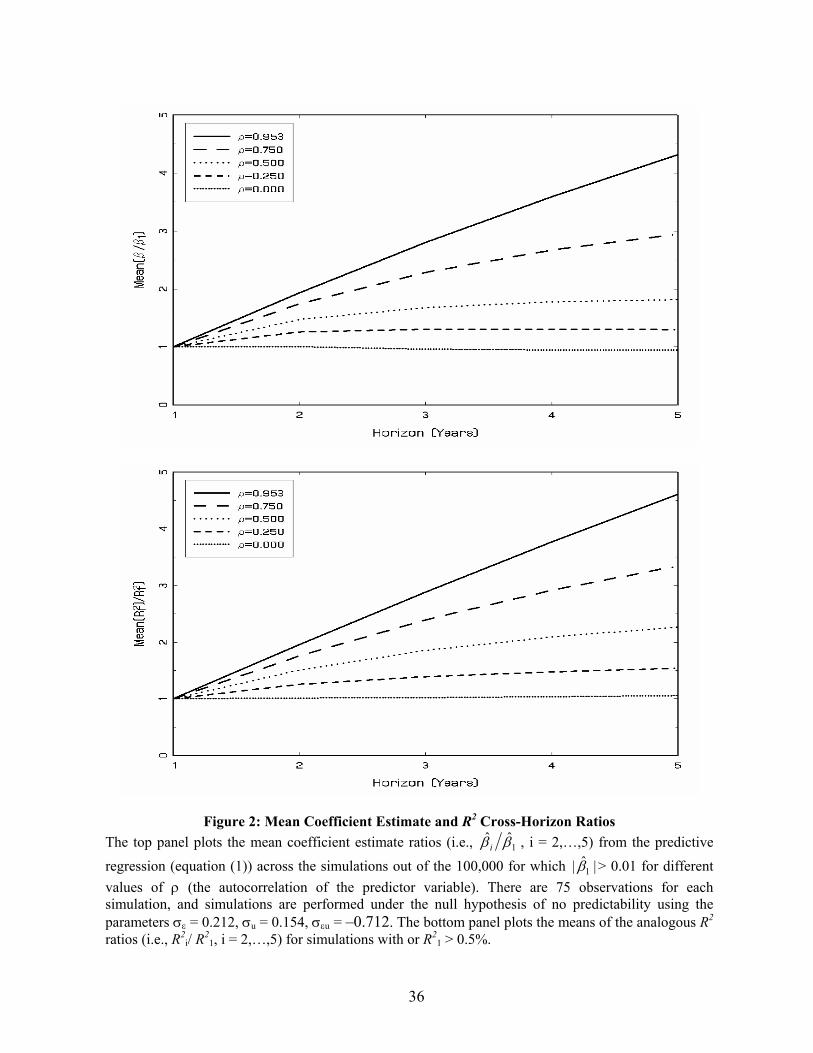
Figures 2A and 2B plot the ratios as a function of the persistence parameter ρ. For large ρ,
both the coefficient estimates and R2s increase linearly with the horizon, with fairly steep
slopes (albeit not quite one-for-one). As persistence drops off, the slope diminishes
dramatically. For ρ = 0, the ratio plot is actually flat. Nevertheless, given the high persistence
of the predictive variables used in practice, the more relevant ratios would be those
corresponding to steep slopes. These graphs show the mean of the ratio; however,
understanding the full distribution allows us to examine whether the actual estimates fall
within the empirical null distributions.
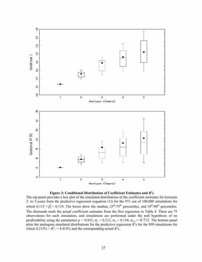
To better understand the statistical likelihood of the observed evidence in light of the
distribution of the various relevant coefficients under the null hypothesis, Figures 3A and 3B
show box plots of the distribution of the multiple-horizon coefficient estimates and R2s
conditional on the 1-year coefficient estimate and R2 being close to the actual values (i.e., β̂ =
0.131 and R2 = 5.16%). The box plots show the median, the 25th and 75th percentiles, and the
more extreme 10th and 90th percentiles of the distribution. Several observations are in order.
First, consistent with Figures 2A and 2B, the percentiles linearly increase at a fairly steep rate.
Second, the actual values of the coefficients and R2s from the data (marked as diamonds in the
graph) lie uniformly between the 25th and 75th percentiles. Given some amount of sampling
error, the hypothesis of no predictability produces precisely the pattern one would expect in
the coefficients under the alternative hypothesis. Because the sample sizes are relatively small,
the presence of sampling error is almost guaranteed. Third, the plots show that what matters is
the magnitude of the coefficient at short horizons. In the voluminous literature on stock return
predictability in finance, no researcher has ever considered the short-horizon evidence to be
remarkable.
19
III. Empirical Evidence
The theory and corresponding simulation evidence in Section II suggests that it will be very
difficult to distinguish between the null hypothesis of no predictability and alternative models
of time-varying expected returns that involve persistent autoregressive processes. The reason is
that sampling error produces virtually identical patterns in both R2s and coefficients across
horizons. However, this finding does not necessarily imply that joint tests will not distinguish
the null from other alternatives. Recall that the null hypothesis implies highly correlated
regression coefficient estimators, which induce the coefficient pattern. Even with
unremarkable coefficient estimators, yet nonconforming coefficient patterns, one might find
strong evidence against the null hypothesis of no predictability.
In this section, we look at a number of commonly used variables to test the predictability
of stock returns. For stock returns, we use the excess return on the value-weighted (VW)
CRSP portfolio, where excess returns are calculated at a monthly frequency using the 1-month
T-bill rate from the CRSP Fama risk-free rate file. For predictors, we use the log dividend
yield on the CRSP VW index, three other payout yields adjusted for repurchases and new
equity issues, the log earnings yield on the S&P500, the default spread between Baa and Aaa
yields, the term spread between long-term government bond yields and T-bill yields, the log
book-to-market ratio, the aggregate equity share of new issuances, and the 1-month T-bill
yield.8
8 See Boudoukh, Michaely, Richardson, and Roberts (2005) for a detailed description of the various measures of payout yield. The data for the first 4 variables are available on Michael Roberts’ website http://www.finance.wharton.upenn.edu\mrrobert\public_html\Research\Data. See Goyal and Welch (2003) for details on variables 5 to 8. We thank Amit Goyal for graciously providing the data. See Baker and Wurgler
20
The regression analysis corresponds to equation (1), and covers return horizons of 1 to 5
years over the period 1926–2004. We use the same number of observations for each horizon;
therefore, the predictor variables span the period 1925–1999 (75 observations) when
available.9 For each set of multiple-horizon regressions, we calculate the coefficient, its
analytical standard error (using equation (2)), its asymptotic p-value, and its simulated p-value
under an AR(1) with matching parameters.10 The AR(1) coefficient used in the simulations is
the estimated first-order autocorrelation, corrected for the small sample bias (Kendall (1954)),
TC1
11ˆ31ˆˆ ρ
ρρ+
+= . (9)
In addition, we conduct a joint Wald test across the equations, using both asymptotic and
simulated p-values. Throughout, asymptotic standard errors, p-values, and test statistics are
calculated using the uncorrected sample autocorrelation function. The results are reported in
Table 4.
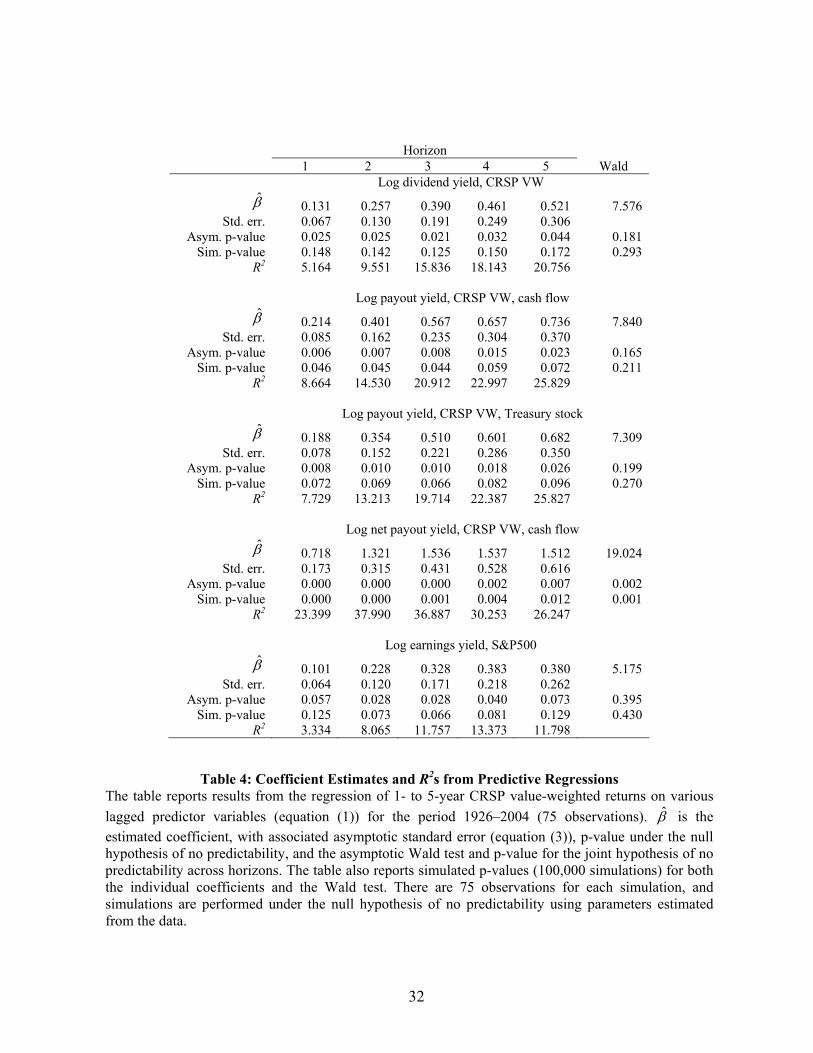
Most of the series show the much-cited pattern of increasing coefficient estimates and
corresponding R2s. For the dividend yield, the payout yield including total repurchases, the
payout yield including treasury stock-adjusted repurchases (all on the CRSP VW index), the
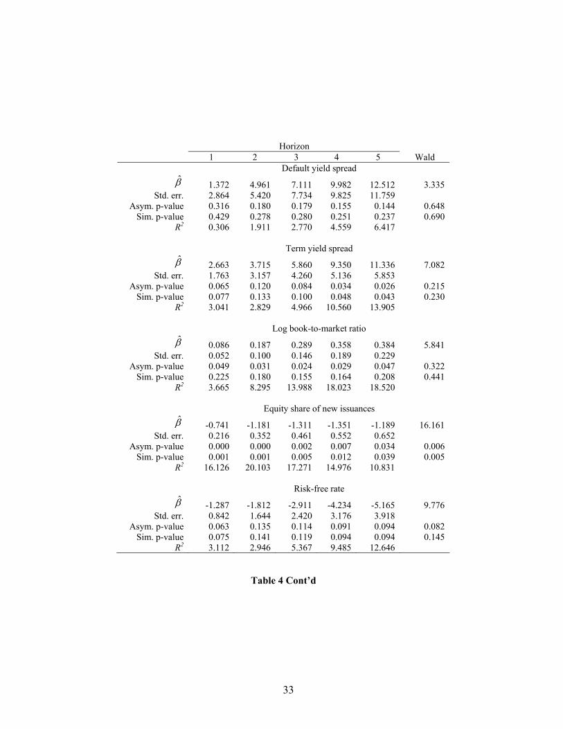
earnings yields on the S&P500, the default spread, the term spread, the book-to-market ratio,
and the risk-free rate the increases in R2 from the 1-year to the 5-year horizon are 5.16% to
20.76%, 8.66% to 25.83%, 7.73% to 25.83%, 3.33% to 11.80%, 0.31% to 6.42%, 3.04% to
(2000) for a description of the equity share of new issuances. The data are available on Jeff Wurgler’s website http://pages.stern.nyu.edu/~jwurgler/. The 1-month T-bill yield comes from the CRSP Fama risk-free rate file. 9 The four payout yield series start in 1926 (74 observations) and the equity share series starts in 1927 (73 observations). 10 Because the equations involve overlapping observations across multiple horizons, small sample adjustments for coefficient estimators and standard errors (e.g., Amihud and Hurvich (2004) and Amihud, Hurvich, and Wang (2005)) are no longer strictly valid. As developing methods for our particular regression system lies outside the scope of this paper, we rely on simulated p-values as a correction for both the correlation (e.g., Stambaugh (1999)) and long-horizon (e.g., Valkanov (2003)) biases.
21
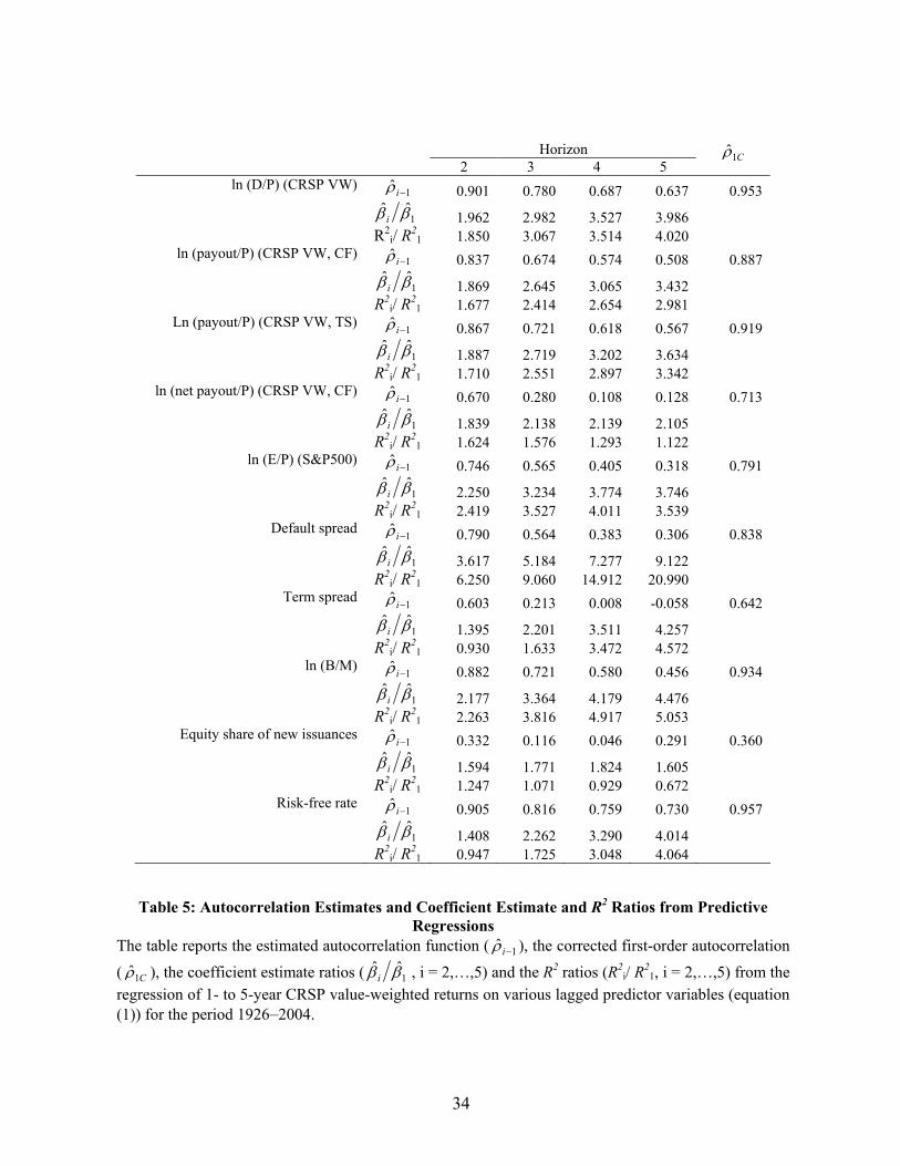
13.90%, 3.66% to 18.52%, and 3.11% to 12.65%, respectively. However, the (corrected)
persistence levels of the associated variables are 95.3%, 88.7%, 91.9%, 79.1%, 83.8%, 64.2%,
93.4%, and 95.7%, respectively (see Table 5). It should not be surprising that many of the
series have significant coefficients using asymptotic p-values across most of the horizons.
Under the null hypothesis, the regressions at each horizon are virtually the same.
Table 5 is an alternative representation of the results in Table 4, i.e., the ratios of the
coefficient estimates and R2s across horizons. For the series cited above (except for the default
spread), the ratios for both quantities are similar to the simulated ratios under the null
hypothesis of no predictability. In all cases, the ratios (and therefore the underlying coefficient
estimates and R2s) increase with the horizon. Thus, the finding that some of the 1-year
regressions are significant, and that the same variables produce virtually identical patterns at
longer horizons, is actually evidence that the annual regression results are due to sampling
error.11 The joint tests confirm this phenomenon by generally producing higher p-values, e.g.,
0.18, 0.16 and 0.20 for the three payout yield variables on the CRSP VW index, 0.39 for the
earnings yield on the S&P500, 0.65 for the default spread, 0.32 for the term spread, 0.32 for
the book-to-market ratio, and 0.08 for the risk-free rate, the only variable significant at the
10% level.
Several observations illustrate the nature of the joint tests. First, consider the regression
results for the dividend yield versus the two payout yield measures on the CRSP VW index.
By almost any eyeball measure, the evidence for the payout yield appears to be stronger. All of
the horizons produce larger coefficient estimates and R2s and lower p-values. While four of the
five p-values are less than 0.02 for the payout yield, none of the coefficients satisfy this

22
criterion for the dividend yield. Nevertheless, the p-value of the joint test for the payout yield
is similar to that for the dividend yield.
Second, the individual coefficient p-values and corresponding R2s of the one marginally
significant variable (out of series cited above) under the joint cross-horizon test, i.e., the risk-
free rate, look less impressive if anything than those for the other series. Yet the significance
level of the joint test is much higher.12 Why? The pattern in the coefficients, while monotonic,
is much less linear and one-to-one than implied by the estimated autocorrelation function. This
result illustrates the power of the joint test to uncover seemingly innocuous differences across
horizons.
Third, the simulated p-values in general show much less significance for both the
individual and joint tests. For example, the risk-free rate is no longer significant at the 10%
level. This mirrors the small sample findings of Goetzmann and Jorion (1993), Kim and
Nelson (1993), and Valkanov (2003). As Tables 1A and 1B show, the correlation pattern
across multiple-horizon estimators is robust to small sample considerations.
Finally, two variables, the net payout yield (i.e., payout yield plus net issuance) and the
equity share of new issuances, are strongly significant across horizons as evidenced by Wald
statistics with p-values of 0.00 and 0.01, respectively. These results are consistent with the
short-horizon findings of Boudoukh, Michaely, Richardson, and Roberts (2005) and Baker and
Wurgler (2000), and show that this evidence continues to long horizons. Of some interest,
while the coefficients and R2s are large across all horizons, the pattern is no longer monotonic.
This finding provides even sharper evidence against the null since the series are positively
11 This conclusion has even greater support once the researcher takes into account the data-snooping arguments of Foster, Smith, and Whaley (1997).
23
autocorrelated at the relevant horizons. With this degree of autocorrelation and the overlapping
horizons, one would have expected a pattern similar to the other predictive variables.
IV. Conclusion
Long-horizon stock return predictability is considered to be one of the more important pieces
of evidence in the empirical asset pricing literature over the last couple of decades (see, e.g.,
the textbooks of Campbell, Lo, and MacKinlay (1997) and Cochrane (2001)). The evidence is
set forth as a yardstick for theoretical asset pricing models and is slowly penetrating the
practitioner community (for two recent examples, see Brennan and Xia (2005) and Asness
(2003)).
Long-horizon predictability has also been documented in other markets, which is perhaps
not surprising, given our analysis. The highly cited work of Fama and Bliss (1987) and Mark
(1995) document results similar in spirit to the ones discussed in this paper for bond returns
and exchange rates, respectively. Both papers involve highly persistent regressors and
document nearly linearly increasing βs and R2s.
In this paper, we show that stronger long-horizon results, in the form of higher βs and
increasing R2s, present little if any independent evidence over and above the short-horizon
results for persistent regressors. Under the null hypothesis of no predictability, sampling
variation can generate small levels of predictability at short horizons. This result is well
known. Our research shows that higher levels of predictability at longer horizons are to be
expected as well.
12 In a multivariate regression framework that includes both dividend yields and the short rate, Ang and Bekeart (2005) find that the short rate has predictive power across multiple horizons.
24
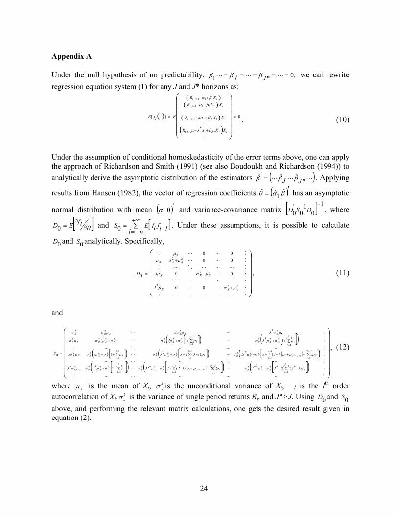
Appendix A
Under the null hypothesis of no predictability, ,0*1 ===== LLL JJ βββ we can rewrite regression equation system (1) for any J and J* horizons as:
( )
( )( )
( )
( )0
*
][
*1*,
1,
111,
111,
=
+−
+−
+−
+−
≡⋅
+
+
+
+
M
M
M
ttJJtt
ttJJtt
tttt
ttt
XXJR
XXJR
XXR
XR
EtfE
βα
βα
βα
βα
. (10)
Under the assumption of conditional homoskedasticity of the error terms above, one can apply the approach of Richardson and Smith (1991) (see also Boudoukh and Richardson (1994)) to analytically derive the asymptotic distribution of the estimators ( )LLL *
ˆˆ'ˆJJ βββ = . Applying
results from Hansen (1982), the vector of regression coefficients )( 'ˆ 1ˆˆ βαθ = has an asymptotic
normal distribution with mean )( '0 1α and variance-covariance matrix [ ] 10
10
'0
−− DSD , where
[ ]θ∂∂
= tfED0 and [ ]∑+∞
−∞= −=l ltftfES0 . Under these assumptions, it is possible to calculate
0D and 0S analytically. Specifically,
+
+
+
=
OLLLLLM
MLL
MLOLLLM
MLL
MLLLOLM
MLL
MLL
22
22
22
00*
00
00001
0
XXX
XXX
XXX
X
J
JD
µσµ
µσµ
µσµµ
, (11)
and
[ ]( ) [ ]( )[ ]( ) [ ]( ) [ ][ ]( )[ ]( ) [ ][ ]( ) [ ]( )
∑ −++∑ ∑++−++∑++
∑ ∑++−++∑ −++∑++
∑++∑+++
=
−
=
−
=
−
=+−
−
=
−
=
−
=+−
−
=
−
=
−
=
−
=
OLLLLLM
MLL
MLOLLLM
MLL
MLLLOLM
MLL
MLL
1*
1
22221
1
**
2221*
1
2222
1
1
*
1*
2221
1
22221
1
2222
1*2221
1
2222222
2222
)*(2**1
)(*1**
)(*)(21
11*1)(
*
0
J
llXXR
J
l
JJ
lllJJlXXR
J
llXXRXR
J
l
JJ
lllJJlXXR
J
llXXR
J
lXXRXR
J
llXXR
J
llXXRXXRXR
XRXRXRR
lJJJJlJJJJJJ
JlJJJJlJJJlJJ
JJ
JJ
S
ρσµσρρρσµσρσµσµσ
ρρρσµσρσµσρσµσµσ
ρσµσρσµσσµσµσ
µσµσµσσ
, (12)
where Xµ is the mean of Xt, 2
Xσ is the unconditional variance of Xt, �l is the lth order autocorrelation of Xt, 2
Rσ is the variance of single period returns Rt, and J*>J. Using 0D and 0S above, and performing the relevant matrix calculations, one gets the desired result given in equation (2).
25
References Ait-Sahalia, Y., and M. Brandt, 2001, “Variable Selection for Portfolio Choice,” Journal of Finance, 56 (4), 1297–1351. Amihud, Y., and C. Hurvich, 2004, “Predictive Regression: A Reduced-Bias Estimation Method,” Journal of Financial and Quantitative Analysis, 39 (4), 813–841. Amihud, Y., C. Hurvich, and Y. Wang, 2005, “Hypothesis Testing in Predictive Regressions,” NYU working paper. Ang, A., and G. Bekaert, 2005, “Stock Return Predictability: Is it There?” Columbia University working paper. Asness, C., 2003, “Fight the Fed Model,” Journal of Portfolio Management, 30 (1), 11–24. Baker, M. and J. Wurgler, 2000, “The Equity Share in New Issues and Aggregate Stock Returns,” Journal of Finance, 55 (5), 2219-2257. Barberis, N., 2000, “Investing for the Long Run when Returns Are Predictable,” Journal of Finance, 55 (1), 225–264 Barberis, N., and R. Thaler, 2003, “A Survey of Behavioral Finance,” The Handbook of the Economics of Finance, ed. North Holland: Amsterdam. Bossaerts, P., and P. Hillion, 1999, “Implementing Statistical Criteria to Implement Return Forecasting Models: What Do We Learn?” Review of Financial Studies, 12 (2), 405–428. Boudoukh, J., R. Michaely, M. Richardson, and M. Roberts, 2005, “On the Importance of Measuring Payout Yield: Implications for Empirical Asset Pricing,” Journal of Finance, forthcoming. Boudoukh, J., and M. Richardson, 1994, “The Statistics of Long-Horizon Regressions Revisited,” Mathematical Finance, 4 (2), 103–120. Brennan, M., and Y. Xia, 2005, “Persistence, Predictability, and Portfolio Planning,” Wharton working paper. Campbell, J., 2000, “Asset Pricing at the Millennium,” Journal of Finance, 55 (4), 1515–1567. Campbell, J., 2001, “Why Long Horizons? A Study of Power Against Persistent Alternatives,” Journal of Empirical Finance, 8, 459–491. Campbell, J., 2003, “Consumption-Based Asset Pricing” in Chapter 13 of The Handbook of the Economics of Finance, ed. North Holland: Amsterdam, 803–881.
26
Campbell, J., and J. Cochrane, 1999, “By Force of Habit: A Consumption-Based Explanation of Aggregate Stock Market Behavior,” Journal of Political Economy, 107 (2), 205–251. Campbell, J., A. Lo, and C. MacKinlay, 1997, The Econometrics of Financial Markets, Princeton: Princeton University Press. Campbell, J., and R. Shiller, 1988, “The Dividend–Price Ratio and Expectations of Future Dividends and Discount Factors,” Review of Financial Studies, 1 (3), 195–228. Campbell, J., and L. Viceira, 1999, “Consumption and Portfolio Decisions When Expected Returns Are Time Varying,” Quarterly Journal of Economics, 114 (2), 433–495 Cochrane, J., 1999, “New Facts in Finance,” Economic Perspectives, 23 (3), 36–58. Cochrane, J., 2001, Asset Pricing, Princeton: Princeton University Press. Cremers, M., 2002, “Stock Return Predictability: A Bayesian Model Selection Perspective,” Review of Financial Studies, 15 (4), 1223–1249. Fama, E., 1998, “Market Efficiency, Long-Term Returns, and Behavioral Finance,” Journal of Financial Economics, 49, 283–306. Fama, E., and R. Bliss, 1987, “The Information in Long Maturity Forward Rates,” American Economic Review, 77, 680–92. Fama, E., and K. French, 1988, “Dividend Yields and Expected Stock Returns,” Journal of Financial Economics, 22, 3–25. Ferson, W., and R. Korajczyk, 1995, “Do Arbitrage Pricing Models Explain the Predictability of Stock Returns?” Journal of Business, 68 (3), 309–349 Foster, D., T. Smith, and R. Whaley, 1997, “Assessing Goodness-of-Fit of Asset Pricing Models: The Distribution of the Maximal R-Squared,” Journal of Finance, 52 (2), 591–607. Goetzmann, W., and P. Jorion, 1993, “Testing The Predictive Power of Dividend Yields,” Journal of Finance, 48, 663–679. Goyal, A., and Welch I., 2003, “Predicting the Equity Premium with Dividend Ratios,” Management Science, 49 (5), 639–654. Hansen, L., 1982, “Large Sample Properties of Generalized Method of Moments,” Econometrica, 50 (4), 1029–1054.
27
Hansen, L., and R. Hodrick, 1980, “Forward Exchange Rates as Optimal Predictors of Future Spot Rates: An Econometric Analysis,” Journal of Political Economy, 88 (5), 829–853. Hodrick, R., 1992, “Dividend Yields and Expected Stock Returns: Alternative Procedures for Inference and Measurement,” Review of Financial Studies, 5(3), 357–386. Kendall, M.G., 1954, “Note on Bias in the Estimation of Autocorrelation,” Biometrika, 41, 403–404. Kim, M.J., and C.R. Nelson, 1993, “Predictable Returns – the Role of Small Sample Bias,” Journal of Finance, 48 (2), 641–661. Kirby, C., 1997, “Measuring the Predictable Variation in Stock and Bond Returns,” Review of Financial Studies, 10 (3), 579–630. Lettau, M., and S. Ludvigson, 2001, “Consumption, Aggregate Wealth, and Expected Stock Returns,” Journal of Finance, 56 (3), 815–849. Lettau, M., and S. Ludvigson, 2005, “Expected Returns and Expected Dividend Growth,” Journal of Financial Economics, 76 (3), 583–626. Lewellen, J., 2004, “Predicting Returns with Financial Ratios,” Journal of Financial Economics, 74 (2), 209–235. Mark, N. C., 1995, “Exchange Rates and Fundamentals, Evidence on Long Horizon Predictability,” American Economic Review, 85 (1), 201–218. Menzly, L., T. Santos and P. Veronesi, 2004, “Understanding Predictability,” Journal of Political Economy, 112, 1–47. Patelis, A.D., 1997, “Stock Return Predictability and the Role of Monetary Policy,” Journal of Finance, 52 (5), 1951–1972 Poterba, J., and L. Summers, 1988, “Mean Reversion in Stock Prices: Evidence and Implications,” Journal of Financial Economics, 22, 27–60. Richardson, M., 1993, “Temporary Components of Stock Prices: A Skeptic’s View,” Journal of Business and Economics Statistics, 11 (2), 199–207. Richardson, M., and T. Smith, 1991, “Tests of Financial Models in the Presence of Overlapping Observations,” Review of Financial Studies, 4 (2), 227–254. Richardson, M., and T. Smith, 1994, “A Unified Approach to Testing for Serial Correlation in Stock Returns,” Journal of Business, 67 (3), 371–399.
28
Richardson, M., and J. Stock, 1989, “Drawing Inferences from Statistics Based on Multi-Year Asset Returns,” Journal of Financial Economics, 25, 323–348. Stambaugh, R.F., 1993, “Estimating Conditional Expectations When Volatility Fluctuates,” NBER Technical Paper 140. Stambaugh, R.F., 1999, “Predictive Regressions,” Journal of Financial Economics, 54 (3), 375–421. Valkanov, R., 2003, “Long-Horizon Regressions: Theoretical Results and Applications,” Journal of Financial Economics, 68 (2), 201–232.
29
Panel A: σεu = –0.712
Coefficient estimates Correlations Horizon Horizon Mean SD Median 2 3 4 5
1 0.055 0.076 0.043 0.966 0.926 0.885 0.843 2 0.106 0.143 0.085 0.980 0.946 0.909 3 0.153 0.203 0.126 0.985 0.957 4 0.196 0.257 0.165 0.988 5 0.235 0.307 0.203 % monotonic 66.02
Test statistics
Size Mean SD Median 10% 5% 1%
Wald 6.227 3.901 5.469 18.507 10.645 3.015 P-value 0.403 0.288 0.361
Panel B: σεu = 0
Coefficient estimates Correlations Horizon Horizon Mean SD Median 2 3 4 5
1 0.000 0.070 0.000 0.960 0.913 0.867 0.823 2 0.000 0.133 0.001 0.977 0.940 0.900 3 0.001 0.194 0.001 0.984 0.954 4 0.001 0.251 0.002 0.988 5 0.000 0.305 0.001 % monotonic 57.30
Test statistics
Size Mean SD Median 10% 5% 1%
Wald 5.949 3.876 5.142 16.813 9.684 2.773 P-value 0.429 0.294 0.399
Table 1: Distribution of Coefficient Estimates and Test Statistics Panel A reports the mean, standard deviation, and median of the coefficient estimates from the predictive regression (equation (1)), and the correlations between these estimates for horizons of 1 to 5 years across 100,000 simulations. “% monotonic” is the percentage of the simulations that produce coefficients that are monotonic in the horizon. Panel A also reports the mean, standard deviation, and median of the joint Wald test statistic (across horizons), the associated p-values, and the percentage of statistics that reject the null hypothesis of no predictability at the 10%, 5%, and 1% levels. There are 75 observations for each simulation, and simulations are performed under the null hypothesis of no predictability using the parameters ρ = 0.953, σε = 0.212, σu = 0.154, σεu = –0.712. Panel B reports the same statistics for σεu = 0 (all other simulation parameters are the same as in Panel A).
30
Panel A: σεu = –0.712
Correlations Horizon Horizon Mean SD Median 2 3 4 5
1 1.833 2.378 0.918 0.949 0.889 0.828 0.767 2 3.469 4.348 1.816 0.969 0.918 0.861 3 4.966 6.041 2.665 0.977 0.933 4 6.337 7.525 3.454 0.981 5 7.600 8.837 4.259 % monotonic 52.21
Panel B: σεu = 0
Correlations Horizon Horizon Mean SD Median 2 3 4 5
1 1.345 1.861 0.618 0.927 0.846 0.768 0.696 2 2.525 3.400 1.203 0.957 0.892 0.821 3 3.614 4.771 1.746 0.969 0.914 4 4.626 5.995 2.280 0.976 5 5.574 7.099 2.790 % monotonic 42.58
Table 2: Distribution of R2s Panel A reports the mean, standard deviation, and median of the R2s from the predictive regression (equation (1)) and the correlations between them for horizons of 1 to 5 years across 100,000 simulations. “% monotonic” is the percentage of the simulations that produce R2s that are monotonic in the horizon. There are 75 observations for each simulation, and simulations are performed under the null hypothesis of no predictability using the parameters ρ = 0.953, σε = 0.212, σu = 0.154, σεu = –0.712. Panel B reports the same statistics for σεu = 0 (all other simulation parameters are the same as in Panel A).
31
Panel A: σεu = –0.712
Coefficient estimate ratios R2 ratios Horizon Mean SD Median # of sim. Mean SD Median # of sim.
2 1.934 0.874 1.919 88,495 1.957 0.813 1.875 62,126 3 2.798 1.894 2.739 88,495 2.880 1.726 2.612 62,126 4 3.592 3.056 3.472 88,495 3.766 2.744 3.237 62,126 5 4.318 4.326 4.139 88,495 4.612 3.821 3.785 62,126 % monotonic 70.38 % monotonic 60.40
Panel B: σεu = 0
Coefficient estimate ratios R2 ratios Horizon Mean SD Median # of sim. Mean SD Median # of sim.
2 1.872 1.154 1.887 87,058 1.905 0.959 1.783 54,599 3 2.620 2.426 2.665 87,058 2.756 1.987 2.400 54,599 4 3.269 3.846 3.350 87,058 3.552 3.082 2.887 54,599 5 3.835 5.357 3.945 87,058 4.299 4.206 3.241 54,599 % monotonic 61.27 % monotonic 49.00
Table 3: Distribution of Coefficient Estimate and R2 Cross-Horizon Ratios Panel A reports the mean, standard deviation, and median of the coefficient estimate and R2 ratios (i.e.,
1ˆˆ ββ i and R2
i/R21, i = 2,…,5) from the predictive regression (equation (1)) across the simulations out
of the 100,000 for which 1̂β > 0.01 or R21 > 0.5%, respectively. “% monotonic” is the percentage of
these simulations that produce coefficient estimates and R2s that are monotonic in the horizon. There are 75 observations for each simulation, and simulations are performed under the null hypothesis of no predictability using the parameters ρ = 0.953, σε = 0.212, σu = 0.154, σεu = –0.712. Panel B reports the same statistics for σεu = 0 (all other simulation parameters are the same as in Panel A).
32
Horizon 1 2 3 4 5 Wald
Log dividend yield, CRSP VW β̂ 0.131 0.257 0.390 0.461 0.521 7.576
Std. err. 0.067 0.130 0.191 0.249 0.306 Asym. p-value 0.025 0.025 0.021 0.032 0.044 0.181
Sim. p-value 0.148 0.142 0.125 0.150 0.172 0.293 R2 5.164 9.551 15.836 18.143 20.756
Log payout yield, CRSP VW, cash flow
β̂ 0.214 0.401 0.567 0.657 0.736 7.840 Std. err. 0.085 0.162 0.235 0.304 0.370
Asym. p-value 0.006 0.007 0.008 0.015 0.023 0.165 Sim. p-value 0.046 0.045 0.044 0.059 0.072 0.211
R2 8.664 14.530 20.912 22.997 25.829 Log payout yield, CRSP VW, Treasury stock
β̂ 0.188 0.354 0.510 0.601 0.682 7.309 Std. err. 0.078 0.152 0.221 0.286 0.350
Asym. p-value 0.008 0.010 0.010 0.018 0.026 0.199 Sim. p-value 0.072 0.069 0.066 0.082 0.096 0.270
R2 7.729 13.213 19.714 22.387 25.827 Log net payout yield, CRSP VW, cash flow
β̂ 0.718 1.321 1.536 1.537 1.512 19.024 Std. err. 0.173 0.315 0.431 0.528 0.616
Asym. p-value 0.000 0.000 0.000 0.002 0.007 0.002 Sim. p-value 0.000 0.000 0.001 0.004 0.012 0.001
R2 23.399 37.990 36.887 30.253 26.247 Log earnings yield, S&P500
β̂ 0.101 0.228 0.328 0.383 0.380 5.175 Std. err. 0.064 0.120 0.171 0.218 0.262
Asym. p-value 0.057 0.028 0.028 0.040 0.073 0.395 Sim. p-value 0.125 0.073 0.066 0.081 0.129 0.430
R2 3.334 8.065 11.757 13.373 11.798
Table 4: Coefficient Estimates and R2s from Predictive Regressions The table reports results from the regression of 1- to 5-year CRSP value-weighted returns on various lagged predictor variables (equation (1)) for the period 1926–2004 (75 observations). β̂ is the estimated coefficient, with associated asymptotic standard error (equation (3)), p-value under the null hypothesis of no predictability, and the asymptotic Wald test and p-value for the joint hypothesis of no predictability across horizons. The table also reports simulated p-values (100,000 simulations) for both the individual coefficients and the Wald test. There are 75 observations for each simulation, and simulations are performed under the null hypothesis of no predictability using parameters estimated from the data.
33
Horizon 1 2 3 4 5 Wald
Default yield spread β̂ 1.372 4.961 7.111 9.982 12.512 3.335
Std. err. 2.864 5.420 7.734 9.825 11.759 Asym. p-value 0.316 0.180 0.179 0.155 0.144 0.648
Sim. p-value 0.429 0.278 0.280 0.251 0.237 0.690 R2 0.306 1.911 2.770 4.559 6.417
Term yield spread
β̂ 2.663 3.715 5.860 9.350 11.336 7.082 Std. err. 1.763 3.157 4.260 5.136 5.853
Asym. p-value 0.065 0.120 0.084 0.034 0.026 0.215 Sim. p-value 0.077 0.133 0.100 0.048 0.043 0.230
R2 3.041 2.829 4.966 10.560 13.905 Log book-to-market ratio
β̂ 0.086 0.187 0.289 0.358 0.384 5.841 Std. err. 0.052 0.100 0.146 0.189 0.229
Asym. p-value 0.049 0.031 0.024 0.029 0.047 0.322 Sim. p-value 0.225 0.180 0.155 0.164 0.208 0.441
R2 3.665 8.295 13.988 18.023 18.520 Equity share of new issuances
β̂ -0.741 -1.181 -1.311 -1.351 -1.189 16.161 Std. err. 0.216 0.352 0.461 0.552 0.652
Asym. p-value 0.000 0.000 0.002 0.007 0.034 0.006 Sim. p-value 0.001 0.001 0.005 0.012 0.039 0.005
R2 16.126 20.103 17.271 14.976 10.831 Risk-free rate
β̂ -1.287 -1.812 -2.911 -4.234 -5.165 9.776 Std. err. 0.842 1.644 2.420 3.176 3.918
Asym. p-value 0.063 0.135 0.114 0.091 0.094 0.082 Sim. p-value 0.075 0.141 0.119 0.094 0.094 0.145
R2 3.112 2.946 5.367 9.485 12.646
Table 4 Cont’d
34
Horizon 2 3 4 5
C1ρ̂
ln (D/P) (CRSP VW) 1ˆ −iρ 0.901 0.780 0.687 0.637 0.953
1ˆˆ ββ i 1.962 2.982 3.527 3.986
R2i/ R2
1 1.850 3.067 3.514 4.020 ln (payout/P) (CRSP VW, CF) 1ˆ −iρ 0.837 0.674 0.574 0.508 0.887
1
ˆˆ ββ i 1.869 2.645 3.065 3.432 R2
i/ R21 1.677 2.414 2.654 2.981
Ln (payout/P) (CRSP VW, TS) 1ˆ −iρ 0.867 0.721 0.618 0.567 0.919
1ˆˆ ββ i 1.887 2.719 3.202 3.634
R2i/ R2
1 1.710 2.551 2.897 3.342 ln (net payout/P) (CRSP VW, CF) 1ˆ −iρ 0.670 0.280 0.108 0.128 0.713
1
ˆˆ ββ i 1.839 2.138 2.139 2.105 R2
i/ R21 1.624 1.576 1.293 1.122
ln (E/P) (S&P500) 1ˆ −iρ 0.746 0.565 0.405 0.318 0.791
1ˆˆ ββ i 2.250 3.234 3.774 3.746
R2i/ R2
1 2.419 3.527 4.011 3.539 Default spread 1ˆ −iρ 0.790 0.564 0.383 0.306 0.838
1
ˆˆ ββ i 3.617 5.184 7.277 9.122 R2
i/ R21 6.250 9.060 14.912 20.990
Term spread 1ˆ −iρ 0.603 0.213 0.008 -0.058 0.642
1ˆˆ ββ i 1.395 2.201 3.511 4.257
R2i/ R2
1 0.930 1.633 3.472 4.572 ln (B/M) 1ˆ −iρ 0.882 0.721 0.580 0.456 0.934
1
ˆˆ ββ i 2.177 3.364 4.179 4.476 R2
i/ R21 2.263 3.816 4.917 5.053
Equity share of new issuances 1ˆ −iρ 0.332 0.116 0.046 0.291 0.360
1ˆˆ ββ i 1.594 1.771 1.824 1.605
R2i/ R2
1 1.247 1.071 0.929 0.672 Risk-free rate 1ˆ −iρ 0.905 0.816 0.759 0.730 0.957
1
ˆˆ ββ i 1.408 2.262 3.290 4.014 R2
i/ R21 0.947 1.725 3.048 4.064
Table 5: Autocorrelation Estimates and Coefficient Estimate and R2 Ratios from Predictive Regressions
The table reports the estimated autocorrelation function ( 1ˆ −iρ ), the corrected first-order autocorrelation ( C1ρ̂ ), the coefficient estimate ratios ( 1
ˆˆ ββ i , i = 2,…,5) and the R2 ratios (R2i/ R2
1, i = 2,…,5) from the regression of 1- to 5-year CRSP value-weighted returns on various lagged predictor variables (equation (1)) for the period 1926–2004.
35
Figure 1: Cross-Horizon Correlations between Coefficient Estimates and R2s The top panel plots the correlation between the coefficient estimate at the 1-year horizon and those at the 2- to 5-year horizons from the predictive regression (equation (1)) across 100,000 simulations for different values of ρ (the autocorrelation of the predictor variable). There are 75 observations for each simulation, and simulations are performed under the null hypothesis of no predictability using the parameters σε = 0.212, σu = 0.154, σεu = –0.712. The bottom panel plots the analogous correlations for the predictive regression R2s.
36
Figure 2: Mean Coefficient Estimate and R2 Cross-Horizon Ratios The top panel plots the mean coefficient estimate ratios (i.e., 1
ˆˆ ββ i , i = 2,…,5) from the predictive regression (equation (1)) across the simulations out of the 100,000 for which |ˆ| 1β > 0.01 for different values of ρ (the autocorrelation of the predictor variable). There are 75 observations for each simulation, and simulations are performed under the null hypothesis of no predictability using the parameters σε = 0.212, σu = 0.154, σεu = –0.712. The bottom panel plots the means of the analogous R2 ratios (i.e., R2
i/ R21, i = 2,…,5) for simulations with or R2
1 > 0.5%.
37
Figure 3: Conditional Distribution of Coefficient Estimates and R2s The top panel provides a box plot of the simulated distributions of the coefficient estimates for horizons 2- to 5-years from the predictive regression (equation (1)) for the 971 out of 100,000 simulations for which 0.115 < 1̂β < 0.119. The boxes show the median, 25th/75th percentiles, and 10th/90th percentiles. The diamonds mark the actual coefficient estimates from the first regression in Table 4. There are 75 observations for each simulation, and simulations are performed under the null hypothesis of no predictability using the parameters ρ = 0.953, σε = 0.212, σu = 0.154, σεu =–0.712. The bottom panel plots the analogous simulated distributions for the predictive regression R2s for the 899 simulations for which 4.215% < R2
1 < 4.414% and the corresponding actual R2s.