8

ISER W

orking Paper S

eries

The Nature and Causes of Attrition in the British Household Panel Survey

S C Noah Uhrig Institute for Social and Economic Research University of Essex

No. 2008-05 February 2008

ww

w.iser.essex.ac.uk

NON-TECHNICAL SUMMARY Why do people participate in surveys? More importantly, why do people participate in on-going studies where they are asked to complete a survey every year? When members of the public are drawn at random to participate in a survey, they cannot be replaced. Some respondents cannot be found by interviewers in the first place. The types of people who cannot be found or refuse to participate are not always random and the extent to which non-random non-participation occurs, the results of the study will be biased against such types of people. This research examines the patterns of survey response amongst a group of people initially participating in an on-going study. I find that people who live in accommodation that is particularly difficult to reach because of things like gated entry systems or shared entrances – such as flats in multi-flat buildings – along with people who are frequently not at home because they work long or odd hours are particularly unlikely to be found year on year when the interviewer calls. At the same time, respondents who are older tend to be more likely to refuse participation in the study even after having provided an interview in an earlier year. On the other hand, respondents with children, particularly young children, and respondents who are highly active socially and in their communities are significantly more likely to remain in the study. These findings are of importance to substantive social researchers in determining how to correct their models of social life using these data to account for the non-random nature of survey non-participation.

The Nature and Causes of Attrition in the British Household Panel Study

SC Noah Uhrig Institute for Social and Economic Research

February 2008 ABSTRACT Panel attrition is a process producing data absent from panel records due to survey non-participation or other data unavailability. I examine the nature and causes of attrition resulting from non-contact and survey refusal in the British Household Panel Study. Focusing on non-response transitions amongst Wave 1 respondents using discrete time transition models, I locate attrition at first non-response over the first 14 waves. Physical impediments to contact, less time spent at home and high likelihood of geographic mobility are predictive of subsequent non-contact. Refusals most often result from lack of interest in the survey and general low motivation to participate. Keywords: Panel attrition; BHPS; survey non-response JEL Codes: C42; C80 Contact: SC Noah Uhrig, ISER, University of Essex, Wivenhoe Park, Colchester, CO4 3SQ, UK; tel. +44(0)1206-873790; email scnuhrig@essex.ac.uk The work reported in this paper is part of the research project “Solving the problem of attrition in longitudinal surveys,” funded under the ESRC Survey Design and Measurement Initiative and directed by John Bynner (ESRC award RES-175-25-0011). Thanks are due to Annette Jäckle, Alita Nandi, Peter Lynn and Harvey Goldstein for helpful suggestions. The support of the UK Longitudinal Studies Centre (ESRC award H562255004) is also gratefully acknowledged.

Social science data sets with repeated observations on the same units are a highly

valuable means of examining the processes of social change. Whether the empanelled

units are organisations, cities, families or individual people – a time series of consistent

measures on the same observational units allows researchers to track types of within-unit

change and ultimately build models of its causes and consequences. Attrition is the process

that leads to absence of data in the panel record as a result of survey non-response or other

data unavailability. Survey non-participation can result from a survey organisation’s failure

to locate and contact sample members on the one hand and non-cooperation with a request

to participate in the survey on the other. Using data from the British Household Panel Study

(BHPS), I examine the nature and causes of attrition, both as a result of non-contact with

sample members and of survey non-cooperation. I adopt a definition of attrition similar to

others who have studied it. I find that factors indicative of physical impediments to contact,

less time spent at home and high likelihood of geographic mobility are predictive of

subsequent non-contact over the life of the panel. I also find the refusals could be viewed

as resulting from lack of interest in the survey and general low motivation to participate. I

begin by outlining what is meant by panel attrition while relating this concept to the general

concept of survey non-participation. I then review the theoretical approaches to the causes

of non-response and review findings from the panel attrition literature within this theoretical

framework. I present the results of several models predicting the rate of attrition,

establishing the similarity between the attrition process in the BHPS and general survey

non-participation. I conclude by briefly discussing outstanding findings that could warrant

further investigation.

1 Motivation Attrition is a problem for panel studies for two reasons. As a panel sample

decreases in size over its duration, the precision of estimates derived from that sample also

decreases (Branden, Gritz and Pergamit 1995; Watson 2003). More importantly, attrition

may not be random. Non-random attrition implies that the sample becomes

unrepresentative as the panel ages and that outcomes of interest may be biased to the

extent that the factors associated with attrition are related to them (Fitzgerald, Gottschalk

and Moffitt 1998; Watson 2003). For these reasons, the present analysis of the covariates

of attrition in the British Household Panel Study (BHPS) serves two related purposes. First,

what factors explain the pattern of unit response in the study? Can established theories of

survey participation account for the attrition process in the BHPS? The second motivation is

derived from the method of accommodating biasing attrition in panel analysis. Observable

factors associated with unit non-response that are not associated with a model’s dependent

1

variable can be used as instruments in correcting for any selection bias due to non-random

non-response (Lepkowski 1989; Lepkowski, Kalton and Kasprzyk 1989). These

observables may also be used in weighting the resulting data to correct for the changing

representativeness of the panel over time (Lepkowski, Kalton and Kasprzyk 1989). For

these reasons, the second purpose of this study is to document the covariates of unit non-

response so that substantive researchers can take into account the changing nature of the

sample in producing their estimates.

2 Identifying Attrition In any panel study where people are the units of observation, attrition is the

permanent loss of data for a sampled individual due to non-participation in the study (Lynn

et al. 2005; Zabel 1998). By definition, attrition is an absorbing state, and in this way differs

from non-response generally (Hawkes and Plewis 2006). Interim unit non-response – i.e.,

individuals dropping out for a single wave before returning again at some subsequent wave

– is different from attrition as data for sample members continues after a gap. The causes

of interim unit non-response may be different from attrition although distinguishing interim

non-response from attrition is always time dependent leading to difficulty in analysis. Panels

of finite length can clearly identify the point of attrition as no further data collection efforts are

attempted even with interim unit non-response. Panels of indefinite length are burdened by

the future behaviour of sample members as attrition cannot be distinguished from interim

non-response without clear rules defining when non-response is attrition.

Survey organisations running a panel of indefinite length might clearly realise survey

efficiencies when repeated non-responders – either by reason of non-contact or refusal –

are not re-issued to field (Laurie, Smith and Scott 1999; Taris 2000; Watson 2003). For this

reason, some indefinite length panels require that panel participants be dropped from

subsequent interview attempts upon either the first or second instance of non-contact or

non-cooperation (Fitzgerald, Gottschalk and Moffitt 1998; Hawkes and Plewis 2006; Lillard

and Panis 1998; Stoop 2005). In this case, attrition is the first instance of non-response

during the life of a panel for the panel participant. Other long running panel studies continue

to attempt to locate respondents with whom contact has been lost or re-issue refusing

respondents in an attempt to secure compliance at later waves (Jones, Koolman and Rice

2006; Laurie, Smith and Scott 1999; Watson 2003). Re-issuance of non-responders also

may happen as a matter of course in household panels where some household members

cooperate with the survey attempt while others continue to refuse. Attrition under these

2

circumstances occurs at the point of last response – noting that “last” response is a

temporally slippery term1.

The methods literature contains many examples of modelling attrition in panel

surveys (e.g.,Behr, Bellgardt and Rendtel 2005; Branden, Gritz and Pergamit 1995;

Fitzgerald, Gottschalk and Moffitt 1998; Hawkes and Plewis 2006; Jones, Koolman and Rice

2006; Lepkowski and Couper 2002; Lillard and Panis 1998; Watson 2003). The bulk of this

work treats the first instance of unit non-response during the course of the panel as panel

attrition whether the design of the survey generating the data actually drops such

respondents from continued survey attempts2. By modelling the first instance of non-

response, these studies favour data analysts requiring a balanced panel. This approach

also makes modelling the attrition process tractable in that no right censoring can occur.

Unit non-response, here, is an absorbing state by analytic definition, whether subsequent

response occurs during the fieldwork period under investigation or not.

By agreed survey rules, all Original Sample Members (OSMs) of the BHPS are

reissued for interviewing at each successful wave until a point of adamant refusal or long-

term non-contact (Taylor et al. 2007). Long-term non-contact is defined by rule to be 4

failed interview attempts. Adamant refusal is judged on the description of the refusal from

survey interviewers. In some instances, sample members who have not been contacted for

more than 4 waves will return to a household in which a cooperating OSM resides. Also, an

OSM who previously refused adamantly may still reside with a cooperating OSM and could

decide to be interviewed. Since all re-interviews are attempted with all OSMs at each

successive wave wherever they may live, some sample members organisationally defined

as attritors may in fact return to the study for interviewing. For the purposes of this present

study, I follow the example in the methods literature and treat attrition as the first instance of

unit non-response and disregard any remaining data available for a given respondent.

3 Attrition and Non-Response Theory Given that attrition is a special case of non-response occurring in panel surveys, the

literature on survey participation sheds light on the underlying process. Groves and Couper

(1998) advanced a general theory of non-response that was later translated for use in

1 It should be noted that reasons other than attrition due to non-contact or refusal may result in no data for respondents. These might include a sample member’s death or movement out of scope, abroad for example. 2 Jones et al., (2006) and Hawkes and Plewis (2006) also model non-response at each subsequent wave regardless of continued participation up to the non-responding wave.

3

modelling panel attrition by Lepkowski and Couper (2002). The original formulation divided

the survey process into first making contact with sample members and then inducing

cooperation with the survey request. In applying this approach to panel studies, Lepkowski

and Couper’s reformulation divided making contact with sample members into the problem

of first locating or tracking respondents and secondly contacting respondents conditional on

location. Non-response is really the product of these separate processes, tracing failure,

failure to contact and survey non-cooperation – all of which may operate independent of one

another (Nicoletti and Peracchi 2005). The literature on panel attrition, however, rarely

differentiates amongst these processes, focusing instead on the general absence of data

regardless of the processes generating it.

3.1 Locating and Contacting Respondents Non-contact is the result of failure to either locate sample members or to make

communicative contact with sample members given that they have been located. Locating

respondents is a simple matter of ensuring that contact details exist, including name,

address and any other information through which communication might be established, that

the survey organisation holds these details and that they are accurate for sample members.

Locating respondents in a cross-sectional survey is fairly straightforward as the relevant

information is often implied in the sampling procedure. In longitudinal or panel studies,

locating the same sample members over time depends largely on the likelihood of

respondent geographic mobility, their willingness to be found given a move and the survey

organisation’s efforts in tracking sample members over time. Additionally, aspects of survey

design can influence this process significantly. For example, the length of the study, length

of time between contact, tracing procedures, following rules, and amount of stable contact

information gathered can be associated with the likelihood of a move occurring during the

study period or with the likelihood of positively locating a sample member given a move.

The characteristics of sample members and their households may also indicate the

likelihood of moving home or being found despite moving home. The likelihood of

geographic mobility, itself, depends, in part, on the degree of household stability and

community attachment – both can be indicated by characteristics of the respondent and/or

their household (Groves and Couper 1998; Lepkowski and Couper 2002; Stoop 2005).

Assuming a panel sample member is located – and in the same location as at

previous waves – making contact is relatively straightforward since the sample member had

been contacted in the past. A sample member’s contactability is the likelihood for them to

be in productive communicative interaction with the interviewer at any point during the

interviewing period (Groves and Couper 1998). Failure to make contact with a located

4

sample member can occur, however, for generally one of three reasons. First, contactability

depends on respondent’s patterns of being physically present at the place where contact is

to be attempted (e.g., home, office, somewhere else). Next, any physical impediments to

making contact with respondents affects their contactability. Locked or shared entrances to

apartment buildings, vicious dogs, caller identification equipment are some examples of

physical impediments associated with inability to make contact with a respondent in their

household. Finally, contact depends on the survey organisation’s effort in making contact.

The effect of these sorts of factors should be lessened in the household panel case because

a survey was conducted at the respondent’s residence in the past. Since these factors will

have once been accommodated, further interviewing can be conducted in light of the

knowledge of at-home patterns, physical impediments and the amount of effort and the time

at which previous contact was made.

3.2 Survey Cooperation Groves and Couper (1998) elaborate extensively on the ability of interviewers to

induce survey cooperation in respondents. Much of their theoretical approach rests on

social-psychological processes that under-gird the decision to comply with the survey

request. They outline four heuristic principles that may be operative in a respondent’s

reasoning. First, the consistency principle suggests that one should be more willing to

comply with requests for behaviours that are consistent with a position to which the are

committed – e.g., once the interviewer has their foot in the door, a sample member is more

likely to comply with the survey request. Next, the scarcity principle suggests that

compliance is more likely if compliance might secure a scarce opportunity – e.g., “This is

your chance to tell us what you think”. Social validation is the third principle and it implies

that compliance depends on whether one perceives whether similar others would also

comply. An example if this type of reasoning might run something like ”Those who are kind

are helpful, I think I’m a kind person so therefore I will be helpful in this instance”.

Obviously, such thinking is not as explicit in the face of the survey request but is instead a

taken for granted thought pattern. Finally, the liking principle might be operative if

compliance is most likely when the requester is liked – “I like this nice lady at the door, so I

think I would enjoy speaking with her.” Liking another can depend, in part, on similarity of

dress, attitude, the use of praising and compliments (Groves and Couper 1998).

Other aspects of the survey and the survey process itself can affect propensity to

cooperate with the survey request. These might include the thematic coverage of the

survey, the nature of the sponsoring organisation, characteristics of the sample member

themselves and situational factors including whatever the respondent is doing at the time

5

the interviewer calls on the household. Some respondents may affect a fairly complex

decision making calculus incorporating cost-benefit analysis, compliance with principles of

social exchange or authority demands along with the decision making heuristics outlined

above. Expert interviewers can tailor the participation request by raising or lowering the

saliency of various factors depending on the verbal and non-verbal cues given by

respondents (Groves and Couper 1998; Groves, Singer and Corning 2000).

Groves and Couper (1998) further elaborate upon the rationale for the effects of

various respondent and/or household demographic characteristics on non-response. Here

they draw on what might be called endowed characteristics of respondents which affect their

response propensity. They argue that individuals who are social isolates are less likely to

respond than those who are socially integrated into their communities, regardless of

interviewer tailoring. Feelings of social isolation suggest that such respondents are not

governed by the norm of civic duty or feelings of cohesion with larger society (Groves,

Singer and Corning 2000). Those with a greater normative disposition are most likely to

participate in surveys irrespective of any incentive structure that might otherwise alter the

cost-benefit balance of participating (Groves, Singer and Corning 2000). Moreover, social

isolates tend to have a lower sense of social obligation to others and hence when a stranger

requests participation in a survey, feelings of obligation to participate are not operative

resulting in lower levels of participation (Groves and Couper 1998). This perspective has

been used to explain survey non-response among ethnic minority groups, through the

hypothesis of encroaching infirmities on explaining lower participation among the elderly,

and as a reason for gender related non-response (Groves 1990; Groves and Couper 1998).

3.3 Findings in the Literature Groves and Couper (1998) hypothesise that various demographic variables are

indirect measures of social psychological constructs, rather than direct causal influences on

participation including age, sex, household structure, relationship status, employment status,

etc…. At the same time age and other known demographic characteristics can proxy other

respondent characteristics, such as health or geographic mobility, which cannot be

ascertained directly when modelling response propensity.

3.3.1 Age. For household surveys, older respondents should be easier to locate and

contact in their home because they tend to have a lower chance of moving home and to

spend more time in their home than others (Stoop 2005). Younger panel members are

more difficult to locate because moving home is more frequent – e.g., moving away to

university – while once located are more difficult to contact because they tend to live in

6

dwelling units where contact is more difficult – such as multi-unit flats – and to spend more

time out of the home (Stoop 2005). A large body of empirical investigation finds that both

the elderly and the young are more likely to not be contacted (Behr, Bellgardt and Rendtel

2005; Branden, Gritz and Pergamit 1995; Cannell et al. 1987; Cheesbrough 1993; DeMaio

1985; Dohrenwend and Dohrenwend 1968; Foster 1998; Foster and Bushnell 1994; Goyder

1987; Groves 1989; Groves and Couper 1998; Hawkins 1975; Lillard and Panis 1998; Lynn

and Clarke 2002; Stoop 2005; Watson 2003).

Concerning survey cooperation, some argue that the elderly are more likely to

maintain norms of civic duty which suggests greater likelihood of survey cooperation

(Dillman 2000; Groves and Couper 1998; Groves, Singer and Corning 2000). At the same

time, younger sample members might be less likely to cooperate because norms of social

obligation might be less strongly felt (Groves and Couper 1998; Stoop 2005). The problem

of encroaching infirmities – the increasing chance of finding older sample members with

health problems – suggests a greater likelihood of situational refusal amongst the elderly

(Groves, Singer and Corning 2000; Jones, Koolman and Rice 2006). Research suggests,

however, that the elderly are more likely to refuse the survey request than younger sample

members (Brehm 1993 ; Cheesbrough 1993; Foster and Bushnell 1994; Goyder 1987;

Groves and Couper 1998; Hawkins 1975; Lepkowski and Couper 2002). Once health is

controlled, however, Jones et al. (2006) find no effect of age suggesting that age effects on

non-response are largely a matter of contactability rather than cooperativeness.

3.3.2 Household Structure. The nature and extent of relationships in the household can

affect the likelihood of locating and/or contacting panel members. Single person households

are more difficult to contact because there is a greater chance of finding the home empty

when the interviewer calls (Brown and Bishop 1982; Couper 1991; Foster 1998; Foster and

Bushnell 1994; Foster et al. 1993; Goyder 1987; Groves and Couper 1998; Jones, Koolman

and Rice 2006; Kemsley 1976; Kordos 1994; Lyberg and Lyberg 1991; Nicoletti and

Peracchi 2002; Wilcox 1977). The presence of children signals greater community

integration – that is, less social isolation – implying locating and contacting sampled

households with children in them is easier than single person households or households

without any children in them at all (Groves and Couper 1998). Indeed, the presence of

children and their ages is associated with lower levels of attrition in the NLSY (Branden,

Gritz and Pergamit 1995), PSID, SIPP and the ECHP (Watson 2003; Zabel 1998).

Aside from the size and composition of households, the nature of the relationships

amongst household members can indicate survey cooperation. Married couples tend to be

7

more residentially stable (Lepkowski and Couper 2002) and, indeed, the married tend to

have lower non-response in the PSID (Fitzgerald, Gottschalk and Moffitt 1998; Lillard and

Panis 1998) and the ECHP (Behr, Bellgardt and Rendtel 2005; Watson 2003). Single –

those never married – are more likely to refuse survey participation more generally

(Fitzgerald, Gottschalk and Moffitt 1998; Foster 1998; Foster and Bushnell 1994; Goyder

1987; Lillard and Panis 1998; Nathan 1999; Nicoletti and Peracchi 2002). Those marrying

young are more likely to attrite in the NLSY (Branden, Gritz and Pergamit 1995), although

early marriage may signal higher geographic mobility which itself is associated with lower

contactability. Similarly, those who are separated tend to be more likely to non-respond in

the PSID (Lillard and Panis 1998) although transitioning out of marriage predicts attrition in

the PSID as well (Fitzgerald, Gottschalk and Moffitt 1998). Behr et. al (2005) find that the

widowed are less likely to attrite than married – this is most likely a masked age effect.

Jones et. al, (2006) however find no effect of marital status.

3.3.3 Gender. Research suggests that women are less likely to be non-responders than

men and that fewer women are lost in panel studies than men (Brehm 1993 ; Foster 1998;

Goyder 1987; Lepkowski and Couper 2002; Lynn et al. 1994). Women’s higher

contactability in household surveys may be due to a greater likelihood of caring for children

in the home – the presence of whom signal greater contactability generally as noted above.

Also men have traditionally worked outside the home and hence are less likely to be found

at home for interviewing (Groves 1990).

Some evidence suggests that men are less likely to cooperate with survey requests

in cross-sectional surveys than women (Lindström 1983; Smith 1983). Groves (1990)

suggests this results from gender roles in mixed sex households. Women tend to manage

the relationship between the household and the outside world. That is, women tend to be

responsible for answering the telephone or front door when someone calls upon the house

(Groves and Couper 1998). For these reasons, women may be more amenable to

interacting with people outside the household, be in the position to answer a request for

being surveyed and hence would be the person most likely to grant the survey request

(Groves 1990; Groves and Couper 1998). Nevertheless, most studies tend to find no real

gender effect in cooperativeness itself (Goyder 1987; Groves and Couper 1998; Stoop

2005).

Within the panel context, although few studies distinguish between cooperation and

contact, there is evidence that men tend to attrite more frequently then women. Lepkowski

and Couper (2002) find that women are more likely to cooperate in the ACL and NES.

8

Similarly, men are more likely to attrite in the NCDS (Hawkes and Plewis 2006) and the

ECHP (Behr, Bellgardt and Rendtel 2005). However, once education, employment, child

care responsibilities and other factors are controlled, Watson (2003) finds no effect of

gender on non-response in the ECHP at all.

3.3.4 Labour Market Activity. Household contactability depends on both the amount of

time spent at home but also patterns of when household members are present in the home.

In addition to the presence of children, patterns of being at home can be affected by

employment commitments outside the home. Sample members who are employed outside

the home are simply less likely to be found at home for interviewing. Anyone employed

greater than full-time would be acutely susceptible to non-contact when contact is only

attempted at the respondent’s home. Thus the presence and amount of work commitments

outside the home tend to predict non-contact generally and in panel surveys in particular

(Branden, Gritz and Pergamit 1995; Cheesbrough 1993; Dunkelberg and Day 1973; Foster

and Bushnell 1994; Goyder 1987; Groves and Couper 1998; Lynn and Clarke 2002).

Simple employment outside the home, either as an employee or self-employed, seems to be

associated with lower levels of non-response in the NLSY (Branden, Gritz and Pergamit

1995), the PSID and the SIPP (Zabel 1998). Those out of the labour market including

sample members in full-time education, those retired or engaged in family care are less

likely than employed to non-respond in the ECHP (Behr, Bellgardt and Rendtel 2005;

Watson 2003). Job instability is also implicated in greater non-contactability in the NCDS

(Hawkes and Plewis 2006) and NLSY (Branden, Gritz and Pergamit 1995), although Jones

et al (2006) found no effect of unemployment.

3.3.5 Housing, Mobility and Neighbourhood Attachment. Aspects of both the housing

unit itself along with the attachment people have to it and its surrounding neighbourhood are

strong indicators of contactability in both cross-sectional and in panel studies.

Neighbourhood attachment is largely indicative of likely future geographic mobility, which

itself is a strong predictor of non-response (Goyder 1987; Lepkowski and Couper 2002).

For this reason, measures of neighbourhood attachment may be strong predictors of

subsequent non-response in panel studies.

Regarding the nature of the housing unit itself, Groves and Couper (1998) show that

the mere presence of any physical impediment to accessing respondents is associated with

lower contact rates. They find that sampled households residing in structures with any

physical impediment to contact have non-contact rates nearly 3.5 times higher than sampled

households without any physical impediments (1998, pp. 89; see also Lynn 2003).

9

Housing tenure can suggest the stability of sampled households and hence contact

is easier to maintain with households which own their home. Zabel (1998) finds home

owners less likely to attrite than renters in both the PSID and SIPP. Lepkowski and Couper

(2002) find that renters are less likely to respond at the second waves of both the ACL and

the NES. Similarly, Watson (2003) finds renters more likely to attrite in ECHP.

Lepkowski and Couper (2002) specifically examine the effects of community

attachment and social integration. Indicators included frequency of talking on the telephone,

visiting friends and attending meetings outside the home as well as satisfaction with one’s

home and whether the respondent provided care for someone outside the home. They find

that respondents with greater intensity on each of these measures tended to be easier to

locate. Further, they found that talking on the telephone, attending meetings outside the

home and caring for a friend or relative outside the home predicted survey cooperation.

3.3.6 Physical Health. Locating and contacting respondents can be affected by poor

health. The onset of long-term health conditions, for example, can dampen contactablity to

the extent such conditions remove respondents from their homes in pursuit of care (Groves

and Couper 1998; Jones, Koolman and Rice 2006). At the same time, transient health

conditions or the onset of long-term conditions can affect the willingness of respondents to

cooperate with the survey request when they are found at home (Groves and Couper 1998).

Oddly, few studies of attrition actually incorporate measures of respondent’s prior health in

determining response propensities. Lepkowksi and Couper (2002) find that those less

satisfied with their health in the ACL are more likely to become non-responders. Regarding

the relationship between physical health and non-response in panel surveys, Jones et. al.

(2006) found that relative to those self-reporting good or excellent health, those reporting

less than good health in Wave 1 of the BHPS become less likely to respond at later waves

of the study. They also find that the presence of functional limitations predicts eventual non-

response but that self-reported disability surprisingly is unrelated to survey cooperation.

They do not model these health effects dynamically, however, so poor initial health predicts

eventual non-response rather than the onset of poor health. Considering that they find no

age effect, one might assume that health status measured at Wave 1 is actually masking

age related attrition.

3.3.7 Socio-Economic Status including income and education. Groves and Couper

(1998) argue that socio-economic status (SES) has either a direct negative or curvilinear

effect on survey cooperation. Their perspective assumes governments conduct or sponsor

surveys. They argue that the underlying mechanism accounting for the relationship

10

between SES and survey cooperation is respondent’s attitude towards the government as

operative in a system of social exchange. They reason that higher SES groups feel they are

continuously tapped for resources and hence owe the government nothing extra. Low SES

groups could go either way. First, since low SES groups are more likely to receive benefits

or other state support, they feel a duty to help the government in its data collection activities.

Alternatively, low SES groups may feel the injustice of on-going disadvantage and when

confronted by the survey interviewer as an agent of a more advantaged group they may be

less willing to cooperate.

Together with occupation, SES is often indicated by educational attainment or

income level or some combination thereof (Grusky 2001). Regarding education, Groves

and Couper (1998) distinguish its effects from SES generally while at the same time saying

nothing about income. They explain that those with greater educational attainment are more

likely to see the utility of survey participation and the links between participation and the

greater good. For this reason, one should find higher response rates amongst those with

higher levels of education. Since higher educational attainment is often associated with

higher SES, though not necessarily, this approach would be at odds with their general SES

argument implying lower cooperation rates for high SES respondents. It should be noted

that occupational group has never been hypothesised nor ever shown to be related to non-

response.

Empirical findings for income and education do not necessarily comport with Groves

and Couper’s approach. Refusals are more likely amongst those with low incomes while

less likely amongst those with higher incomes (Allen et al. 1991; Brehm 1993 ; DeMaio

1985; Fitzgerald, Gottschalk and Moffitt 1998; Goyder 1987; Iyer 1984; Nathan 1999; Ross

and Reynolds 1996). Survey non-cooperation is also most likely amongst those who are

less educated (Cheesbrough 1993; Dillman 2000; Dunkelberg and Day 1973; Foster and

Bushnell 1994; Goyder 1987; Lynn et al. 1994; Nathan 1999; O'Neil 1979; Robins 1963;

Wilcox 1977). Groves and Couper’s approach has nothing to say about the relationship

between SES – as either income or education – and non-contact. In Britain, a number of

studies find that high income households are more likely to be non-contacts (Cheesbrough

1993; Dunkelberg and Day 1973; Foster and Bushnell 1994; Goyder 1987; Lynn and Clarke

2002).

In the panel context, the findings for income and education as specific indicators of

SES are more disparate. Although the NLSY follows young people, Brandan et al (1995)

found that having no earnings predicts non-response, but among those with earnings the

11

amount of earnings has no effect. On a panel with a broader age profile, Fitzgerald et al

(1998) find, in the PSID, a linear negative effect of earnings on probability of ever non-

responding among male householders, no effect for women, but having no earnings predicts

non-response for female householders. Modelled dynamically, they further find that high

earners are less likely to attrite but that those experiencing a large shift in earnings over

time, either positive or negative, are more likely to become attritors. We might suppose that

a large shift in earnings signals some other structural change in the household

geographically or in terms of employment. Their finding suggests that household financial

instability of any type, positive or negative, predicts non-response. These results do not

seem supportive of Grove and Couper’s social exchange approach to these types of factors,

however.

Analyses of non-response in the ECHP by both Behr et al. (2005) and Watson

(2003) provide the most evidence for the relationships posited by Groves and Couper.

Watson finds that the main source of earnings matters but not always the amount of

earnings. Income from pensions, benefits, and private sources rather than from labour, are

all associated with higher attrition in the ECHP generally. Behr et al. revise the income

measure and find that both the top and bottom of the income distribution are more likely to

attrite across ECHP countries. These findings imply the curvilinear relationship between

SES and survey cooperation in that those in the middle of the SES distribution are more

likely to have income from earnings than from other sources. Watson goes on to find,

however, that the lower portion of the income distribution is associated with higher attrition in

northern European countries while the higher end of the income distribution is associated

with attrition in southern European countries, broadly speaking. Although Watson and Behr

et al differ in modelling strategies, the similarity in their results suggest that the relationship

between SES and survey response exists but that it perhaps depends on broader socio-

cultural factors observable cross-nationally.

Concerning the link between education and non-response in the panel context,

Branden et al (1995) find that educational enrolment decreases non-response in the NLSY,

and that attainment is negatively related to non-response among men, but not women.

Similarly, Jones et al. (2006) find that respondents with higher achieved qualifications have

higher response probabilities over the life of the panel. At the same time both Lillard &

Panis (1998) and Fitzgerald et al. (1998) confirm that the less educated are more likely to

attrite in PSID. Watson (2003) also finds that more education is associated with less

attrition in northern Europe. However, Watson also finds that less education is associated

12

with less attrition in southern Europe implying that the participation explanation proffered by

Groves and Couper may not be operational in all societies.

3.3.8 Prior Survey Experiences. In addition to respondent characteristics, aspects of

respondents’ prior experiences with being interviewed, particularly in an on-going panel

study, can influence their likelihood of continued cooperation – including the survey

organisation’s ability to locate respondents and maintain contact with them.

With longitudinal or panel studies, a respondent’s prior survey experience will affect

their willingness to cooperate with each successive survey request (Laurie, Smith and Scott

1999; Lepkowski and Couper 2002). Respondents’ general cooperativeness with prior

interviews seems to indicate a willingness for further participation wherever it has been

examined (Branden, Gritz and Pergamit 1995; Laurie, Smith and Scott 1999; Lepkowski and

Couper 2002). Initial refusal, however, is countered in several panel studies with refusal

conversion programmes. Undergoing refusal conversion is highly predictive of eventual

non-response in the NLSY (Branden, Gritz and Pergamit 1995) and in the BHPS (Burton,

Laurie and Lynn 2006; Laurie, Smith and Scott 1999). The effectiveness of retaining

respondents depends on the refusal reasons, with situational refusals less likely than survey

related refusals to be lost from studies long-term (Burton, Laurie and Lynn 2006)

Incentivisation is also a factor in determining subsequent non-response (Laurie, Smith and

Scott 1999) although Groves et al (2000) find that those maintaining stronger norms of civic

duty are less influenced by the size and nature of incentives. The running time of the

interview can signal greater respondent burden or it can signal a greater commitment by

respondents to engaging with the interviewer. Interview length has, however, been found to

be associated with lower levels of attrition (Branden, Gritz and Pergamit 1995; Zabel 1998)

while a greater number of questions answered is also indicative of lower attrition (Hawkes

and Plewis 2006). It would seem, then, that longer interview running time and more

questions answered indicates respondent interest rather than overburdening. Thematic

coverage of a study – either asking sensitive questions or covering topics of variant saliency

in a population – is implicated in respondent interest and subsequent participation. Brenden

et al (1995) found that questioning marijuana use does not predict non-response in the

NLSY, but that those refusing income questions are more likely to subsequently non-

respond. Lepkowski & Couper (2002) find that interest in politics predicts greater

cooperation in the panel component of the NES.

In addition to the above discussed features of the survey design itself, prior interview

experiences are largely tempered through the interviewer. As the main contact between a

13

survey organisation and the respondent, aspects of the interviewer and interviewer

behaviour often colour the experience of respondents. Indeed, Zabel (1998) reports that for

SIPP participants, one of the main reasons for continuing participation listed by respondents

is liking the interviewer. Burton et al (2006) report from anecdotal evidence that both

respondents and interviewers prefer to have the same interviewer returning each year for

the interview. Some research finds interviewer continuity is highly predictive of subsequent

panel cooperation (Behr, Bellgardt and Rendtel 2005; Branden, Gritz and Pergamit 1995;

Laurie, Smith and Scott 1999; Pannenberg and Rendtel 1996; Zabel 1998), however the

reasons for this are unclear. Consistency in interviewer could represent some form of liking

process inducing cooperation, yet the observed interviewer effect could be a spurious result

of living an area with high interviewer turnover such as a central city – associated with non-

response in its own right (Campanelli and O'Muircheartaigh 1999; Groves and Couper 1998)

– or geographic mobility – associated with loss due to tracking failure (Laurie, Smith and

Scott 1999; Lepkowski and Couper 2002). However, Laurie et al, (1999) found that the

strongest effect of a change of interview was among those who have not moved in the prior

year suggesting that the rapport built up over time between respondents and their

interviewers may be a significant factor in respondent retention.

3.3.9 Other Findings. Groves et al (2000) suggest that survey cooperation may be more

likely for those maintaining a sense of civic duty. Normative feelings of civic duty may be

indicated by a number of opinion items although little prior research explores whether the

opinions or values respondents hold predict the likelihood of non-response. Opinions and

attitudes may be expressive of respondent interest in the themes and topics covered by a

survey. For example, Lepkowski and Couper (2002) find that those less interested in

politics were more likely to non-respond in the panel component of the NES. A more direct

test of this civic duty thesis may be derived from measures of social participation. Civic

mindedness may be more prevalent amongst people highly engaged in community affairs.

It follows that respondents highly engaged in community life would be more willing to

provide survey data. Lepkowksi and Couper (2002) also generally find that social

participation inhibits subsequent panel non-participation.

4 The British Household Panel Study: Sampling and Fieldwork Drawing on the survey participation literature, I explore survey participation in the

British Household Panel Study. Here, I analyse only the response patterns of initial

individual respondents over the first 14 waves of the panel. I first describe the initial

sampling design before discussing the fieldwork procedures.

14

The British Household Panel Study (BHPS) is a multi-purpose panel that began in

1991. Original sample units consisted of 8,217 addresses drawn from the small users

Postcode Address File (PAF) as a sampling frame. The frame itself comprised Great Britain

south of the Caledonian canal and excluded Northern Ireland. In a first stage of selection,

250 postcode sectors were selected as the primary sampling units (PSUs) from an implicitly

stratified listing of all sectors on the PAF using a systematic sampling method. In a second

selection stage, fieldwork delivery points, which are approximately equivalent to addresses,

were sampled from each selected PSU using an analogous systematic procedure. The

Interviewers conducted a third stage of selection at the household level. BHPS defines a

household as “one person living alone or a group of people who either share living

accommodation OR share one meal a day and who have the address as their only or main

residence.” Interviewers selected households from delivery points at the time of fieldwork,

excluding non-residential addresses and institutions, using two rules: (a) any point

containing up to three households, include all; and (b) for more than three households at a

delivery point, select up to three households using a random selection procedure defined on

the total number of households present.

At Wave 1, interviewers sought to contact and solicit interviews with all resident

household members who were aged 16 or over on 1st December 1991. Interviewers

attempted to secure proxy interviews for eligible household members who could not be

interviewed because of illness or absence. The net result was an interviewed sample of

10,264 individuals at Wave 1 including 352 proxies. Subsequent to Wave 1, interviews were

sought with all Wave 1 respondents – including proxies – wherever they may be located.

Interviews were also sought with all resident members of the household in which

interviewers found a Wave 1 respondent. In subsequent waves, interviewers posted an

advance letter to all eligible respondents just before expecting to call on the household. The

letter informs respondents that the interviewer will call on the household within the next

week. Any prior wave firm refusals are excluded from fieldwork. Interviewers made a

minimum of six calls at each sampled address before it was considered a non-contact;

interviewers were encouraged to make further calls, if possible.

4.0.1 Types of Interviews From Wave 1 to Wave 8, data was gathered through a face-to-

face PAPI interview, with CAPI being introduced from Wave 9. The individual interview

normally takes between 30 and 40 minutes. Interviewers also administer a household

questionnaire lasting approximately 10 minutes to one person in the household. All

individual respondents are also asked to complete a confidential paper questionnaire.

Interviewers collect proxy data for a small number of respondents who may be absent long-

15

term from the household or too ill to participate. Beginning at Wave 3, a selected set of

highly skilled interviewers would attempt to convert current wave refusals or previous wave

adamant refusals to a full-interview. Refusal conversion follows an established protocol, full

details of which are outlined by Burton et al. (2006) and also can be found in the BHPS

documentation (Taylor et al. 2006). In the event that a refusing respondent cannot be

converted to a full interview, refusal conversion interviewers offer a short 10-minute

telephone interview. For the present study, I consider both telephone interviews as well as

proxy interviews as study compliance and not attrition.

5 Analytic Methods To understand the characteristics of attrition in the BHPS, I estimated a set of

transition models treating the non-response process as akin to any sort of survival process

(see also Watson 2003). Original sample members were considered “responders” so long

as they gave complete interviews – either full, proxy or telephone – wave on wave (i.e.,

survive within the panel). A respondent transitioned into a state of being an “attritor” once

they failed to provide an interview because they could not be located or contacted, or

refused the survey request. The non-response hazard rate, then, was the probability of

“attriting” and was modelled as a function of observable covariates to understand what

factors might explain non-response over the life of the panel (Allison 1984; Nicoletti and

Peracchi 2005). While a person could conceivably become ineligible for interview by reason

of moving abroad or into an institution of some sort, or otherwise decide to non-respond at

any point in time, the measure of response or non-response occurs at the point of attempted

contact between the interviewer and respondent. Given wave on wave interviewing, with

repeated attempts to contact a given respondent at each wave, the response outcome is

best viewed as a state measured at the close of fieldwork. Hence the way time was

conceived in these models was discrete rather than continuous with any non-response

outcome recorded once at each wave.

In a discrete-time transition model, the hazard is modelled as a function of time and

a set of covariates. The hazard rate is typically expressed as the odds, ϑ , of an event, Y,

defined as the ratio of the probability of the event Y occurring to the probability of that same

event not occurring:

)1Pr(1)1Pr()1(=−

===

YYYϑ

16

Given that probabilities range from 0 to 1, the odds can range from 0, when Pr(Y = 1) = 0, to

infinity when the Pr(Y = 1) = 1. By taking the natural logarithm of the odds, we obtain the

logit:

ϑeL log=

In this paper, I model the logit transformation of the probability of responding in a given

wave (Lt). The independent variables are modelled as a linear function using maximum

likelihood estimation. In short, this discrete-time transition approach adopts standard logistic

regression methods with the data transformed into person-years and pooled with time

entered as a covariate (Allison 1984; Hanushek and Jackson 1977; Watson 2003):

14,...2;110 =+++= −− tXL ititttit εβββ

t indicates time and Xit-1 represents lagged covariates for each respondent i. The non-

response probability is modelled as a function of lagged covariates – the prior year’s

information is used to predict the likelihood of subsequent non-response. I did not test any

interactions between independent variables and time. Note that each individual may appear

more than once in the data set, thus the standard errors in the model need to be adjusted to

take account of clustering at the individual level which results in a within-person correlated

error term (Watson 2003). In the present analysis, I specify the Primary Sampling Unit

(PSU)3 as the clustering variable (Kreuter and Valliant 2007). I pooled data from the first 14

waves, thus modelling non-response at Wave 2 through to Wave 14. Covariates were

measured from Waves 1 to 13.

[TABLE 1 HERE]

All Wave 1 respondents – including those interviewed by proxy at Wave 1 – form the

sample over which this analysis proceeded. Table 1 accounts for the fieldwork outcomes of

all Wave 1 respondents between Wave 1 and Wave 14. As previously mentioned, the

refusal conversion process could result in a respondent with a telephone interview rather

than a proxy or full-interview from Wave 3. I included telephone respondents in the risk set

at each wave, thus I considered any type of interview – full, proxy or telephone – as an

interview for analytic purposes. While the number of proxy interviews with Wave 1

respondents has decreased over the life of the panel, the number of telephone interviews at

each wave has been more erratic. At Wave 14, 5,288 Wave 1 respondents were

3 Please see (Taylor et al. 2006) for a further discussion of the BHPS sampling structure including the definition of primary sampling units.

17

interviewed in full, or approximately 51.5 percent of all Wave 1 respondents. The modelling

strategy is based on pooled data where each case is retained if their interview outcome is a

full-interview, a proxy, a telephone interview, a non-contact or a refusal. I treated any

respondent who was not issued to field in a given wave because they moved abroad, died,

were a long-term or adamant refusal, long-term non-contact or otherwise ineligible for

interview under the following-rules of the BHPS as censored in this analysis. Censoring was

handled by removing cases from the risk set in the wave that they became ineligible for

interview. Since I modelled non-response as an absorbing state, those moving back into

scope – say, returning from abroad, deciding to be interviewed after a period of refusal –

were not re-introduced into the sample history.

Non-response could be due to failure to locate, failure to contact or failure to secure

an interview with any given survey respondent. Here I present results for models with three

different dependent variables. The first models the rate of general non-response. The

second and third sets of models predict the non-contact hazard, i.e., Y = NC, and the hazard

rate of refusal given contact, i.e., Y = (REF | NC)4. I do not distinguish between failure to

locate a respondent, e.g., they remain untraced, and non-contact because the timing of

untraced respondents is not clear in the resulting data. Some non-contacts in any given

wave, for example, may actually be respondents for whom the contact information is no

longer valid. This may not become apparent immediately but instead only after several

waves. I combine non-contacts with failures to locate respondents for purposes of analysis.

Also, BHPS survey staff may not be able to verify whether a respondent has died between

waves. A small proportion of listed non-contacts will in fact be ineligible for interview due to

death. At Wave 10, a search for death certificates yielded an updating on this status for

several respondents who will have been listed as long-term non-contacts at prior waves.

5.1 Time Dependence Figure 1 shows the hazard rate of initial non-response – i.e., the attrition rate – for

BHPS Wave 1 respondents over the first 14 waves. The solid black line indicates the rate of

non-response, while the dashed line shows the rate of non-contact and the dotted line

shows the refusal rate. We can see that the attrition rate is highest over the first 5 waves of

the panel before levelling off from about Wave 5 through Wave 11. From Wave 12 onwards,

the attrition rate increases. This increase in attrition of Wave 1 respondents after Wave 12

may be due to at least two reasons. First, the cohort of Wave 1 respondents is not

refreshed with younger respondents who matriculate into the study by turning 16. As the

4 The refusal model treats wave non-contacts as censored and therefore these cases are excluded from the refusal analysis at the wave of non-contact.

18

pool of initial Wave 1 respondents, ages, they may be more likely to either refuse or be lost

through non-contact – even temporarily – for reasons of ill-health or aging. This could

increase the hazard of non-response for initial respondents later in the panel. Second, as

the panel ages, Wave 1 respondents may feel they have done enough to support the survey

and may feel a greater motivation to refuse participation in the study after 10 or more years

of providing data regardless of their health.

[FIGURE 1 HERE]

As with the general non-response rate, non-contact and refusal are both initially quite

high before levelling off between about Wave 5 and Wave 10 though these rates are not

high overall. During the initial four waves of the study, refusal rates are higher than non-

contact rates suggesting that those who are predisposed not to cooperate with an ongoing

survey request drop out early during the life of a panel. Non-contact rates, though higher

over the initial few waves than later in the panel, remain relatively constant for Wave 1

respondents over the life of the panel. Refusal is more likely, but this too reaches a steady

state from about Wave 5 onwards. It should be noted that unobserved heterogeneity could

produce specific patterns of time-dependence (Allison 1984). Heterogeneity across

individuals that are not observed and therefore not incorporated into the model tend to

produce evidence of declining rates in models of this sort even if the hazard rate of interest

should not decline as a function of time (Heckman and Singer 1982). However, since the

attrition rate – generally as well as due to non-contact or refusal -- for Wave 1 BHPS

respondents is effectively U-shaped, increasing after Wave 10, unobserved heterogeneity is

unlikely to present problems for this analysis.

Testing various time specifications I settled on a fully flexible time specification as

shown in Table 2. The first column contains the results for a model of non-response,

generally, while the remaining two columns contain results for models of non-contact and

refusal given contact respectively. The fully flexible specification uses a dummy variable for

each wave. This results in an effect coded specification of time with Wave 13 as the omitted

category.

[TABLE 2 HERE]

As indicated by Figure 1, the non-response rates are highest at the beginning of the panel

then drop over the life of the panel, then rebound from about Wave 8 onwards (though recall

that these time dummies should be interpreted relative to Wave 13 rates). Note that the

refusal rate is higher in the first wave than the non-contact rate. Specifically, the odds-ratio

19

for Wave 1 in the refusal model suggests that refusal at Wave 2 is nearly 5.5 times more

likely than at Wave 14 (e.g., = 1.706, p < 0.001, e^b 1.706 = 5.507 in the refusal model), but no

more nor no less likely, with few exceptions, from about Wave 5 onwards. Similarly, non-

contact is about 4.9 times more likely at Wave 2 than at Wave 14 ( = 1.599, p < 0.001,

e

^b

1.599 = 4.948 in the non-contact model), with a steady pattern over the life of the panel from

about Wave 5. The rise in non-response after Wave 10 is largely due to a combination of

both non-contact and refusal at about Wave 11 onwards. Note the mildly significant

coefficients at Wave 10 and Wave 12 for both non-contact and refusal given contact.

6 Substantive Findings Tables 3 through 11 contain results for models with covariates from specific thematic

domains. I have organised the results by thematic domain rather than around substantive

themes derived from the literature on response and non-response to highlight the

relationship between variables often used for substantive research and their relationship to

non-response. I discuss each table in turn, summarising the findings with respect to the

literature on non-response where the results address a point in this literature. Within each

section, I include descriptions of how covariates are measured and the meaning of the

various response categories for each covariate where necessary.

Prior research suggests that item non-response for certain types of items predicts

subsequent unit non-response in panel surveys (Branden, Gritz and Pergamit 1995; Nicoletti

and Peracchi 2005). To retain cases and test whether item non-response does in fact

predict unit non-response, I incorporated for most, if not all, covariates a category

representing missing data on the given item. Recall that I include proxy and telephone

respondents as being at risk for subsequent non-response. Some items are not asked of

proxy or telephone respondents because both of these questionnaires are abridged versions

of the full questionnaire. For this reason, the missing category for some variables will

indicate questionnaire type rather than any meaningful aspect of item non-response. To

control for this, I incorporate indicators of questionnaire type in all models. This means that

item non-response indicators for any substantive variable reflects the association of item

missing data and subsequent response propensity rather than masking a mode effect in

response propensity.

Some covariates are derived from questions that are not asked at each wave. At the

same time, the type of model I have estimated required complete data. For each item not

20

repeated at a given wave, I used the value from the most recent administration of the item.

In instances where the response was missing, this was similarly carried forward to complete

the data set.

With few exceptions, each table presented here takes the same form. The first three

columns contain results of models with the rate of non-response as dependent variable.

The next three columns include results from models predicting the rate of non-contact. The

final three columns report results of models predicting the rate of refusal. Within each set,

the first column presents the “Bivariate” relationship between the covariate and the rate.

This is not really a bivariate relationship, but instead the relationship between this covariate

and the dependent variable with only time and interview mode also controlled in the model.

I do not report the time and interview mode coefficients in each table as they largely do not

change from model to model. The “Domain” model in the second column presents results

from a model that includes all the covariates within the thematic domain covered by the

table while excluding any covariates from other thematic domains. The thematic domains

include:

• Demographics, region and geographic mobility • Household Structure including marital status, household size and the presence of

children • Individual health status and service usage • Housing characteristics as well as neighbourhood attachment • Interview conditions • Labour market participation, socio-economic status and financial standing • Opinions and political preferences • Social participation and religiosity

The final column within each set presents results from a “Multi-domain” model. This is a full-

model which includes covariates from all thematic domains however only the covariates

from the relevant domain are presented together.

6.1 Non-Response as a Function of Demographics, Region and Geographic Mobility Table 3 and Table 4 contain results from models incorporating measures of

demographic characteristics. Table 3 reports the results from models regressing the hazard

rate of non-response, non-contact and refusal on various individual demographic

characteristics, geographic region and geographic mobility. Table 4 contains results from

models incorporating measures of relationship status, household size and household

structure. Many of the covariates presented in Table 4 are highly related to one-another, for

example overall household size is the sum of the number adults plus number of children and

a single household is a household of size one. For these reasons, not all variables are

21

included in the domain or multi-domain models presented in Table 4. This section reports

and discusses these results in turn.

[TABLE 3 HERE]

6.1.1 Birth Cohort. Non-response theory suggests that non-contact will be greater among

younger respondents. Older respondents are more likely to be cooperative out of a sense of

civic duty while younger survey members will be more likely to refuse cooperation for

reasons of a lower sense of obligation. I use birth cohort as a measure of respondent age

because age is collinear with wave in the model. Those born in 1970 or after are the

omitted category. We see that in the general non-response model, an inverted-U shape

across the birth cohorts, those born prior to 1920 are no more nor no less likely to non-

respond than those born in 1960 or after while those born between 1920 and 1959 are less

likely to be non-respondents. The multi-domain non-response model indicates that those

born between 1940 and 1949 are the least likely to non-respond ( = -0.371, p < 0.001).

Comparing these effects to the results for non-contacts and refusals, we see that age

predicts non-contact across age groups rather more than refusal. Across the board, the

negative effects for birth-cohort mean that the highest non-contact rate is for those born in

1970 or after. Note that the multi-domain non-contact model shows that those born between

1920 and 1929 are about 75 percent less likely to be lost through non-contact compared to

those born in 1970 or later ( = -1.380, p < 0.001, e

^b

^b -1.380 = 0.252). Further, across the

cohorts chronologically toward 1970, the coefficients monotonically decrease in magnitude.

This means that non-contact is more likely for younger respondents and that this effect

might largely be monotonic. Note the exception for respondents born before 1920 where

the coefficient of -0.595 (p < 0.001) suggests the oldest of the old are slightly less

contactable than other ages. Interestingly, refusals are more likely among the oldest age

groups. Those born before 1920 are about 53.1 percent more likely to refuse than those

born after 1970 ( = 0.426, p < 0.01, e^b 0.426 = 1.531 in the multi-domain refusal model) while

those born between 1920 and 1929 are about 32.7 percent more likely than respondents

born after 1970 to refuse ( = 0.283, p < 0.05, e^b 0.283 = 1.327). These results confirm the

theoretical predictions about the relationship between age and non-contact and age and

survey cooperation. Moreover, these findings tend to be consistent with findings from

studies of other longitudinal data sets which find a positive relationship between non-

response and age.

22

6.1.2 Gender. Consistent with prior research, I find that women are less likely to non-

respond than men. The “bivariate” and domain specific models suggest that women are

about 10 percent less likely to non-respond than men ( = -0.116, p < 0.001, e^b -0.116 = 0.890,

= -0.121, p < 0.001, e^b -0.121 = 0.886 respectively) . However, this effect disappears in the

multi-domain model notably with the addition of respondent employment status (results not

shown). This implies that men and women are no less likely to non-respond, but that the

patterns of response observed for women have more to do with sex differences in

employment patterns. We might expect, then, that women and men are equally difficult to

contact since employment outside the home theoretically limits contactability with household

members. This notion is not supported, however. Women remain significantly more

contactable than men – being about 12.5 percent less likely to be a non-contact than men all

things considered ( = -0.133, p < 0.01, e^b -0.133 = 0.875 in the multi-domain model). There is

no difference between men and women in the likelihood of refusal once all other factors are

controlled. Above and beyond any effect of employment outside the home as well as the

presence of children, women remain easier to contact than men and no different from men

in their propensity to cooperate with the survey request. These data support the approach

outlined in Groves and Couper (1998) who suggest a gendered division of household labour

which militates in favour of female contactability.

6.1.3 Race. Race is entered as a simple dichotomous variable indicating whether the

respondent is white or non-white. The sample otherwise under-represents non-white

Britons and so meaningful analyses of different ethnic groups cannot be conducted. We see

that being non-white is a highly significant predictor of non-response in the “bivariate” and

domain specific models. However, once other factors are controlled the effect of race is

reduced and remains marginally significant in the multi-domain model ( = 0.665, p < 0.001

in “bivariate” model vs. = 0.304, p < 0.01 in multi-domain model). Disaggregating this

effect into non-contacts and refusals, we see that maintaining contact with non-white

respondents is the main problem. Non-whites remain approximately 52.8 percent more

likely to be lost due to non-contact than whites, all things considered ( = 0.529, p < 0.001,

e

^b

^b

^b

0.529 = 1.697). Once other factors are controlled in the multi-domain refusal model, the

effect of race disappears altogether. The race effect is attenuated when interviewer rated

cooperativeness is included in the general non-response model (results not shown).

However, the remaining evidence does not suggest that non-white respondents are more

likely to refuse the survey request when asked than white respondents.

23

6.1.4 Region. Region is entered as a series of regional indicators with London as the

omitted category. When region is included in the model controlling for other demographic

covariates shown in Table 3 (domain model) various regions are significantly less likely to

non-respond subsequently than London notably the Southeast, Southwest, East Anglia, and

the North/Northeast. Supposing the regions found to be no different from London in this

model have a higher population density in common, this finding comports with the literature

suggesting that interviewing is generally more difficult in highly urban areas (Groves and

Couper 1998; Stoop 2005)5. In the multi-domain non-response model, however, only the

coefficient for East Anglia remains significant with an associated odds-ratio indicating those

living in East Anglia are about 31.7 percent less likely to non-respond than Londoners ( = -

0.381, p < 0.05, e

^b

-0.381 = 0.683). When the non-response effect is split into non-contact and

refusals, the multi-domain models show that region has no effect on non-contact but the

effect for East Anglia remains in the refusal model ( = -0.360, p < 0.05)^b 6. While the

domain specific non-contact model shows some effects for various regions, the multi-

domain model shows no effect of regional at all. The addition of housing structure, in this

model, seems to be the factor that reduces the effect of region (results not shown). The

regions, therefore, must vary in housing structure such that once housing structure is

controlled the regional effect disappears. This must be interpreted with respect to London

as the reference category implying that something about the housing stock in London, per

se, affects the observed response rates. Flats and multi-unit dwellings are associated with

non-contact in other studies of non-response, which are likely dwelling types for

respondents living in London. The specific results for dwelling type are discussed in greater

detail in below.

6.1.5 Geographic Mobility. In the literature, geographic mobility is associated with lower

contactability (Groves and Couper 1998; Lepkowski and Couper 2002; Stoop 2005). This is

of particular concern for panel studies where locating and maintaining on-going contact with

respondents is important. For respondents moving between waves and failing to be

contacted at the latter wave, we cannot know that the move itself has occasioned non-

contact. However, we can identify respondents who have moved within the prior two years

5 No urbanicity measure is available with the BHPS data so we cannot test whether residence in a central city affects response propensities above and beyond any regional variation in response propensities. However, other factors that may be associated with central city living such as possessing a car could indicate a central city-residence. Table 8 contains results for personal access to a car or van. 6 The BHPS is run from the University of Essex which located in the region of East Anglia. For this reason, residents of East Anglia may be more motivated to participate relative to sample members elsewhere.

24

and examine whether this predicts greater odds of subsequent non-response. The history

of geographic mobility, then, may be associated with the likelihood of greater mobility in the

future and hence greater odds of eventual non-contact. In the general non-response model,

we see that those moving in the prior two years are, indeed, more likely to non-respond. In

the multi-domain non-response model we see that among those with a history of moving,

the odds of non-response are increased about 21 percent as compared to others ( =

0.188, p < 0.01, e

^b

0.188 = 1.207). Once non-response is disaggregated into non-contact and

refusal, we see that movers are significantly more likely to be lost due to non-contact than

refusal, as we might expect ( = 0.337, p < 0.001 and = -0.001, n.s., respectively). The

odds of non-contact are increased about 40.1 percent (e

^b

^b

0.341 = 1.401). These findings

broadly comport with theoretical predictions about geographical mobility and non-response

while corresponding with the findings of others regarding geographic mobility.

[INSERT TABLE 4 HERE]

6.1.6 Marital Status. The first five rows of Table 4 contain results for the effect of marital

status with those who are “never married” as the omitted category. Table 4 shows that

controlling for birth cohort and other factors in the multi-domain model, those who are

divorced or widowed are less likely to non-respond, but all other groups are no different from

those never married in their response propensity ( =-0.182, p < 0.05 and = -0.341, p <

0.001, respectively). Interestingly, the “bivariate” relationships indicate that persons married

or partnered have lower odds of non-response, but this association disappears in the multi-

domain model. This is largely due to the inclusion of spousal employment status in the

multi-domain model where having no spouse is the omitted category (see Table 8 for

results). The non-contact models show marital status having no affect on non-contact once

all other factors are controlled. The divorced and widowed remain significantly less likely to

refuse than those never-married ( = -0.335, p < 0.01 and = -0.437, p < 0.001

respectively). These findings differ slightly from the findings for other studies where married

couples are more easily contacted and less likely to refuse cooperation (Behr, Bellgardt and

Rendtel 2005; Fitzgerald, Gottschalk and Moffitt 1998; Lillard and Panis 1998; Watson

2003).

^b

^b

^b

^b

6.1.7 Household Size. Non-response theory and empirical evidence both imply that

survey non-response is less likely amongst larger households (Groves and Couper 1998;

Groves et al. 2002; Lepkowski 1989; Lepkowski and Couper 2002; Nicoletti and Peracchi

25

2005; Stoop 2005). The results (Table 4) show that the “bivariate” relationship between

household size and non-response is in this expected direction ( = -0.071, p < 0.01) with

the likelihood of non-response reduced by about 6.9 percent for each household member (e

^b

-

0.071 = 0.931), although the “bivariate” effect for the number of adults in the household works

the opposite direction ( = 0.117, p < 0.001). At the same time, single households are

significantly more likely to non-respond which corresponds to what might be expected given

the literature ( = 0.215, p < 0.001). In the domain and multi-domain models, I include only

household size as the number of adults and the indicator for a single household vary

strongly with household size. However, once other factors are controlled, the effect of

household size is the opposite – larger households are more likely to non-respond ( =

0.061, p < 0.01 in the domain specific model) – but then disappears in the full-model.

Considering non-contact and refusal, the multi-domain model shows no relationship

between household size and non-contact, but instead a direct positive relationship between

household size and refusal ( = -0.049, p = n.s., and = = 0.124, p < 0.001, respectively).

Indeed, the odds of refusal increase about 13.3 percentage points for each household

member (e

^b

^b

^b

^b

^b

0.124 = 1.132). With respect to arguments about contactability, these findings

contradict the theoretical proposition that large households are more contactable. It may be

the case that the presence of school aged children actually takes parents and families

outside the home. On the other hand, being a household survey, the response burden is

enhanced for larger households and if the burden is high, the members of larger households

may be less willing to provide interviews in subsequent waves.

6.1.8 Children. Theoretically, the presence of children in a household indicates residential

stability and community integration which imply greater contactability on the one hand and a

greater willingness to cooperate with survey requests on the other (Groves and Couper

1998; Lepkowski and Couper 2002; Stoop 2005). The results in Table 4 for the most part

confirm these predictions. Notably, the presence of any children in the household

significantly reduces the odds of non-response for reasons of both non-contact and refusal

( = -0.240, p < 0.001 in the non-response model, = -0.246, p < 0.001 and = -0.229, p

< 0.001 in the non-contact and refusal models respectively). The ages of children is

implicated in theory to have a relationship with the odds of contact and refusal (Groves and

Couper 1998). Specifically, the presence of pre-school aged children but not infants is

expected to enhance the contactability of households (Groves and Couper 1998). Four

variables indicate the presence or absence of children in the household of various ages: 0-2,

^b

^b

^b

26

3-4, 5-11 and 12-15 relative to no children in the household at all. Table 4 shows that while

the results in the “bivariate” models are as expected, the presence of variously aged

children seems to have effects somewhat different than might be theoretically expected.

Contrary to expectation, the results in the multi-domain models show that the presence of

children of various ages has no effect on non-contact. Children, however, reduce the

likelihood of refusal with a significant negative gradient across the age range. That is, the

younger the child the less likely is a refusal ( = -0.545, p < 0.001 for any children aged 0-2,

versus = -0.219, p < 0.05, for children aged 5-11). Note that the presence of children

aged 12-15 is no different from having no children in the household at all in terms of

subsequent refusal. Taken together, these findings support the general approach to non-

response for children – their presence can ease contact with the household but a

respondents propensity for household cooperation is greater if they live with younger aged

children.

^b

^b

6.2 Non-response as a function of Individual Health Table 5 contains the results of non-response, non-contact and refusal regressed on

various health related factors. As with the effect of demographic factors, all models include

a measure of time specified as a series of wave dummies and the interview mode effect

coded with full-interview as the omitted category. The BHPS contains a wide variety of

health indicators as well as measures of health service use. Indicators measuring usage of

various health services tend to be highly collinear. For this reason, the multi-domain models

do not contain a full compliment of health service measures.

Health can have two effects within the context of a general non-response theory.

First, poor health can act against survey cooperation if those with poor health are unfit for or

uninterested in contact with others, particularly a stranger asking them survey questions

about their lives. Thus, poor health may have a strong positive effect on the likelihood of

non-response due to refusal. Second, poor health could occasion trips to the doctor or even

overnight stays in the hospital. For surveys conducted in the home, contactability may be

affected by poor health. Thus, we might expect that poor health leads to non-response

generally, and both refusal and non-contact rates specifically.

[INSERT TABLE 5 HERE]

6.2.1 Respondent Health. The first 14 rows of Table 5 contain results for indicators of

respondent health. These include the count of stated physical health problems, likelihood of

mental health problems as measured by the General Health Questionnaire, whether the

27

respondent smokes, whether the respondent is disabled and the respondent’s self-assessed

health status.

First, the count of health problems has a curious negative effect on non-response,

generally. The more health problems mentioned, the lower the likelihood of non-response.

This effect does not remain in the non-contact model but is mirrored in the refusal model (

= -0.123, n.s.; = -0.187, p < 0.01, respectively).

^b

^b

Next, there appears to be no real association between likely mental health problems

as measured by the General Health Questionnaire, being a smoker or self-reported disability

status. Some slight significance can be noted in the “bivariate” and domain models, but

these effects disappear in the multi-domain models.

Lastly, the relationship between self-assessed health and non-response differs

somewhat from Jones et al. (2006) who examine this relationship with a different modelling

framework. Here, the omitted category is “Excellent” health. The general non-response

model indicates a monotonically increasing likelihood of non-response as the poorer one

rates their own health the more likely they are to non-respond at subsequent waves. Yet

once other factors are controlled in the multi-domain model, this pattern disappears and we

only see some continued significance for poor or very poor health. The non-contact rate

continues to be associated with self-assessed poor health as those indicating their health is

poor remain somewhat likely to be lost due to non-contact ( = 0.424, p < 0.05) but there is

no association between self-assessed health and refusal. The link with age, here, is

important to note. There, the oldest cohorts were found to be more likely to refuse

participation even when health problems and subjective health status were included in the

full-model. Here, health has no independent effect on refusal. The reasons for higher rates

of elderly refusal are, therefore, slightly unclear and may require further investigation.

^b

The sum of these findings does not provide evidence that poor health predicts

refusal as few health indicators are indicative of refusal over the life of the panel. In fact, the

presence of health problems seems to inhibit survey refusal rather than promote it.

However, situational refusal at the point of contact may reflect the onset of ill health or

infirmity between waves that we would not observe in these data. Prior poor health does

seem to predict non-contact, somewhat, suggesting that poor health eventually leads people

out of their households – perhaps in the pursuit of care.

28

6.2.2 Service Use. The results suggesting poor health leads to attrition through non-

contact, however slight, might result from poor health occasioning trips outside the home for

medical care. We would expect, then, that a history of greater use of health care would

predict non-contact as well. I include four indicators of health care usage: number of GP

visits, number of health checks, whether the respondent stayed as an in-patient in the

hospital overnight or longer and whether the respondent used any health services such as

meals on wheels, home help, or a health visitor.

In the general non-response model, we find, relative to those never visiting their GP

in the prior 12 months, a general negative relationship between visiting the GP and non-

response with this effect disappearing in the domain specific model. Along with GP visits,

receiving check-ups is also associated with a reduced likelihood of survey non-response.

Those receiving three or more different types of check-ups such as blood pressure checks,

cholesterol checks, dental checks, eyesight tests, and chest X-rays are significantly less

likely to non-respond, generally ( = -0.236, p < 0.001). Moreover, the coefficient for three

or more check-ups is somewhat larger than the coefficient for one or two check-ups (Wald

X

^b

2 = 3.34, 1 d.f., p < 0.10). Receipt of health checks is also inversely proportional to the

likelihood of non-contact ( = -0.246, p < 0.01 for three or more check-ups) and refusal (

= -0.215, p < 0.05, for three or more check-ups). Note that these respondents may not have

actually been suffering poor or ill health otherwise at the time of interview. Instead,

obtaining more health checks could be indicative of seeking better health and that

respondents actively engaged in self-care this way are more less likely to be survey non-

respondents.

^b

^b

Both being an in-patient and receiving health services might directly indicate

likelihood of being bound to the home for reasons of poor health. Being an in-patient over

night or longer in the year prior may be too distantly removed in time from the contact

attempt and response request to be useful as it largely does not contribute significantly to

these models. The use of health or welfare services is largely unrelated to non-response,

per se, as there is no significant association between service use and non-response in the

multi-domain model. However, use of health services has a significant negative association

with refusal, all things considered ( = -0.166 p < 0.01 in the multi-domain refusal model). ^b

Taking these findings together, it would seem that health has a mild effect on

response propensities in the BHPS. These results suggest that only extremely poor health

29

impairs response and those people actively engaged in managing their health through the

use of health services are easier to retain in the study.

6.3 Non-Response as a Function of Housing Characteristics and Neighbourhood Attachment

Non-response theory suggests respondent contactability is affected by the nature of

housing tenure, the structural characteristics of the dwelling itself and any factors affecting

the local stability of the household unit including place attachment (Groves and Couper

1998; Groves et al. 2002; Lepkowski and Couper 2002; Martin 2007; Watson 2003; Zabel

1998). Table 6 contains results from models incorporating features of respondents’ housing

situation as well as two measures of place attachment.

6.3.1 Housing Tenure. The results presented in Table 6 are consistent with results

elsewhere. Renters are more likely to be lost between waves than those living in owner

occupied accommodation ( = 0.150, p < 0.10 in the multi-domain non-response model;

= 0.361, p < 0.001 in the multi-domain non-contact model). These findings clearly reflect a

greater mobility and less "settled" nature of renting.

^b

^b

6.3.2 Dwelling Type. Physical barriers preventing access to respondents for interviewing

can strongly influence the likelihood of non-response. Respondents dwelling in structures

such as apartment blocks with access to several flats through a shared entrance can be

particularly difficult to reach. I categorised dwelling type into dwellings with their own

entrance, flats and other multi-story units and finally bedsits, institutions, and other

structures. The omitted category, here, is living in a dwelling with its own entrance,

including detached, semi-detached, and terraced houses. The results in Table 6 show that

those dwelling in flats, with any number of flats in the structure, are highly likely to non-

respond relative to those living in a dwelling with its own entrance ( = 0.170, p < 0.01 in

the multi-domain non-response model). Not surprisingly, this is largely due to non-contact

rather than refusal ( = 0.340, p < 0.001 in the multi-domain non-contact model, = -

0.021, n.s. in the multi-domain refusal model). Dwelling in a bedsit, institutional

accommodation or some other type of structure is associated further with non-contact

relative to a house with its own entrance ( = 0.377, p < 0.10). In other words, even in a

panel study, inability to access respondents remains an impediment to contact wave on

wave. Once contact is made, however, those living in flats, bedsits or other dwelling types

are no less likely to cooperate with the survey over time than others as is evidenced by the

lack of any significance in the non-response model for this variable.

^b

^b

^b

^b

30

6.3.3 Place Attachment. Place attachment refers to the feelings of being settled in a given

accommodation or in a local community (Lepkowski and Couper 2002; Martin 2007). Two

measures in the BHPS touch on this concept: whether the respondent would like to move

and whether the respondent likes their neighbourhood. In the general non-response model,

those expressing a desire to move, relative to those not interested in moving are highly likely

to non-respond at the next wave ( = 0.185, p < 0.001 in the multi-domain non-response

model). At the same time, not liking one’s neighbourhood is associated with subsequent

non-response ( = 0.162, p < 0.05 in the multi-domain non-response model). The finding for

desire to move remains in the non-contact model ( = 0.374, p < 0.001) as does the effect of

disliking one’s neighbourhood ( = 0.197, p < 0.05 in the multi-domain non-contact model).

Those expressing a desire to move, additional to any past history of geographic mobility as

shown in Table 3, have non-contact odds about 45 percent higher than others (e

^b

^b

^b

^b

0.374 = 1.454

from the coefficient in the multi-domain non-contact model).

These findings comport with general non-response theory. Any physical impediment

preventing access by interviewers to respondents can significantly affect response

propensities. Once contact is established, however, those living in difficult to contact

residential settings are no less likely to cooperate with the survey. At the same time, low

place attachment signals lower contactability.

6.4 Non-Response as a Function of Interview Conditions Respondents’ prior experience with surveys, either with an on-going panel or with

one-off cross-sectional studies, can affect the likelihood subsequent survey response

(Groves and Couper 1998; Groves, Singer and Corning 2000; Lepkowski and Couper 2002).

Interview length, themes of the study, use of incentives, mode, etc.,… all can affect a

respondents feelings about participation each time a survey request is put to them. Data on

interview length in the BHPS is incomplete so this was not included in these models. The

content of the BHPS questionnaire also rotates across themes or topics over time. This is

broadly collinear with the time specification in these models so any effects of thematic

coverage in the study would be confounded with time. Included here are only measures

largely indicative of the conditions under which the interviews were completed. These

measures gauge to some extent the rapport respondents maintain with interviewers, their

interest in the study and their ability to participate. Included are indicators of interview

mode, the presence and influence of other people during the course of the interview,

completion of tracking information, interviewer assessed cooperativeness and the effects of

31

changing interviewers between waves. Table 7 presents results of non-response models

including these interview characteristics.

[TABLE 7 HERE]

6.4.1 Interview Mode. Most BHPS data is gathered using face-to-face interviews while a

small proportion of interviews are obtained by proxy or over the telephone (Taylor et al.

2007). Both proxy and telephone interviews obtain significantly less data than the full

interview (Burton, Laurie and Lynn 2006; Laurie, Smith and Scott 1999; Taylor et al. 2007).

Much of the item non-response evident in other variables of the models presented in this

paper result from the abridged proxy or telephone instruments. Since I have defined proxy

or telephone interviews as a survey response and a large component of item non-response

is due to the reduced form of data collection with proxies and telephone interviews, I have

included these factors in all domain and multi-domain models as controls.

The initial rows of Table 7 show the relation between interview mode and

subsequent non-response. The “bivariate” relationship between proxy or telephone

interviewing and subsequent non-response is very large. Notably, proxy interviews are

about 5.6 times more likely than face-to-face interview to yield complete non-response at the

subsequent wave ( = 1.730, p < 0.001; e^b 1.730 = 5.64). Similarly, telephone interviews are

associated with a 19.45 times greater likelihood of non-response at the subsequent wave

( = 2.968, p < 0.001; e^b 2.968 = 19.45). With all covariates controlled, these effects disappear

in the multi-domain non-response model most likely as a result of controlling interviewer

rated cooperativeness (see below), amongst other factors. Moreover, the effects of

interview mode have no association with non-contact or refusal all things considered. Note

that both age and health – two factors associated with increased likelihood of a proxy

interview – are controlled.

Proxy respondents and those undergoing refusal conversion yielding a telephone

interview both could eventually provide full interview data gathered through face-to-face

interviewing at a subsequent wave. Having ever given a proxy or ever given a telephone

interview are both still predictive of subsequent non-response. Respondents ever being

proxied are about 1.6 times more likely to subsequently non-respond than others ( = 0.490,

p < 0.001; e

^b

0.490 = 1.632 from the multi-domain non-response model). This effect remains in

the refusal model ( = 0.565, p < 0.001). Ever providing a telephone interview, as expected,

is positively associated with subsequent panel non-response ( = 0.804, p < 0.001).

^b

^b

32

Respondents ever providing a telephone interview, meaning they have ever refused an

interview, are more than 3 times more likely to eventually drop-out of the study than

respondents providing either full or a mixture of full and proxy interviews over the life of the

panel ( = 1.110, p < 0.001; e^b 1.110 = 3.034).

These findings comport with Burton, Laurie and Lynn (2006) who show that the

refusal conversion programme in the BHPS is successful in retaining respondents for a

number of waves, but that those undergoing the programme tend to eventually drop out of

the panel. Similarly, respondents who are proxied may remain in the study for a number of

waves but will eventually drop out.

6.4.2 Presence and Influence of Others. Since, the BHPS is administered face-to-face in

the respondent’s home, the presence of others is often unavoidable as is their influence

over the interview itself. The results in Table 7 show that the presence of others is

associated with lower odds of subsequent non-response ( = -0.138, p < 0.05, in the multi-

domain non-response model), and this relationship remains in the non-contact model ( = -

0.221, p < 0.01) but not the refusal model once other factors are controlled. This appears to

be related to the presence of children in the home (not shown), as children are the most

likely candidates to be present during other interviews. While the presence of others may

have a positive impact on contactability, the influence of others on the survey itself seems to

have a deleterious effect on response propensities. If others influence the interview, itself,

the odds of subsequent non-response are about 25 percent increased ( = 0.224, p < 0.01;

e

^b

^b

^b

0.224 = 1.251). This effect disappears in the non-contact model, but remains in the refusal

model ( = 0.217, p < 0.05). ^b

6.4.3 Tracking. In prior research, failure to provide the name, address and phone number

for someone who would know how to contact the respondent in the event that they cannot

be otherwise found was associated with higher rates of subsequent non-response (Burton,

Laurie and Lynn 2006). That is, failure to provide information about who will know of

respondent’s whereabouts is an effective advance refusal to continued panel participation.

Respondents not providing this tracking information have associated odds of non-response

nearly 2 times higher than respondents providing it ( = 0.701, p < 0.001; e^b 0.701 = 2.016 in

the multi-domain non-response model). While this stable contact information is integral to

maintaining contact with respondents, the effect for providing these details is stronger for

33

refusal than for non-contact ( = 0.455, p < 0.01 in the multi-domain non-contact model; =

0.766, p < 0.001 in the multi-domain refusal model). Partial tracking info is also associated

with eventual refusal but not non-contact. On the one hand, this suggests that providing

partial stable contact information is an advance soft-refusal, perhaps, whereas not

completing is a strong one. On the other, providing less than complete tracking information

could represent an underlying resistance to survey participation generally.

^b

^b

6.4.4 English Language. BHPS interviews are conducted in English7 which means that

any survey respondent not fluent in English could be motivated not to participate at

subsequent waves. Also, one might suppose that non-native English speakers live in less

stable accommodation resulting in lower likelihood of subsequent contactability.

Considering the “bivariate” and domain models, having English language problems predicts

non-response ( = 1.021, p < 0.001 in the “bivariate” non-response model and = 0.549, p

< 0.001 in the domain non-response model). This is largely due to non-contact ( = 1.283,

p < 0.001, = 0.843, p < 0.001, in the “bivariate” and domain models respectively) but not

refusal. All things considered, English language problems affects non-contact only ( =

0.580, p < 0.05). Upon investigation, this attenuated effect results once the respondent’s

race and not having access to a car or van for personal use – a factor associated with urban

living – are included in the model. Note however that English problems are persistent

indicators of subsequent non-contact. A similar set of findings for problems with the self-

completion instrument emerges as some sort of problem with finishing the self-completion

component of the BHPS is associated with subsequent non-contact ( = 0.526, p < 0.05).

Note various “bivariate” and domain effects for requiring assistance and refusing the self-

completion instrument, but that these effects disappear in the full model. Reading these

results together, we might surmise that respondents with a lower ability to participate are

also likely to be difficult to contact. This issue is a larger problem for maintaining contact

with respondents with poor English skills than for inducing them to cooperate with the

interview.

^b

^b

^b

^b

^b

^b

6.4.5 Interviewer Assessed Cooperativeness. Over the course of a 35 to 40 minute

interview, the interpersonal contact between interviewer and respondent can be marked by

quite high rapport. Poor respondent cooperativeness with the interview process itself can

indicate a lack of interest in the survey topics, dislike for the interviewer, mistrust for the

7 Translations into Welsh are required by law but very few interviews are conducted in Welsh.

34

survey organisation or other attitudes. BHPS interviewers rate respondents

cooperativeness at the end of the interview as either Excellent, Good, Fair, Poor or Very

Poor. Very few respondents exhibit Poor or Very Poor cooperation, however, while the

majority of respondents are rated as having Excellent cooperativeness. Table 7 shows the

results of including this measure of respondent cooperativeness with categories set relative

to a rating of ‘Excellent’. There is a general monotonically increasing propensity to non-

respond as cooperativeness declines ( = 0.311, p < 0.001; = 0.833, p < 0.001; and =

1.229, p < 0.001 for Good, Fair and Poor/Very Poor cooperativeness respectively in the

multi-domain non-response model). Poor cooperativeness seems to have a more important

effect for eventual refusal rather than non-contact although the monotonic effects remain

and are strongly significant. This suggests that any respondent disinterest is likely to be

evident to the interviewer and that disinterested or otherwise difficult respondents are, in

fact, more likely to attrite from the study at subsequent waves.

^b

^b

^b

6.4.6 Change of Interviewer. Within the BHPS, every effort is made to return the same

interviewers back to respondents because it is believed that interviewer continuity minimises

the risk of subsequent non-response (Behr, Bellgardt and Rendtel 2005; Burton, Laurie and

Lynn 2006; Laurie, Smith and Scott 1999; Zabel 1998). A change of interviewer may be

occasioned by a respondent move but also interviewer turnover. High interviewer turnover

is noted in some urban areas and both geographic mobility and urban living are theoretically

associated with non-response (Groves and Couper 1998; Laurie, Smith and Scott 1999;

Lepkowski and Couper 2002). Most studies that purport to demonstrate interviewer

continuity effects are non-experimental and might confound interviewer stability with area

effects. At BHPS Waves 2 and 3, interviewer continuity was examined experimentally

(Campanelli, Sturgis and Purdon 1997). Campanelli and O’Muircheartaigh (1999) found no

effect of continuity at Wave 2 but when extended to Waves 3 and 4 significant differences

emerged (Laurie, Smith and Scott 1999). Re-analysis by Campanelli and O’Muircheartaigh

(2002) suggests that apparent non-response differences due to interviewer non-continuity

could result from non-random interviewer attrition. The results from the present analysis in

Table 7 suggest that having a new interviewer is weakly associated with non-response ( =

0.140, p < 0.05 in the multi-domain non-response model), whereas ever having a new

interviewer and the more frequent number of changes in interviewer have no effect.

Splitting non-response into non-contact and refusal, I find that interviewer change has no

effect on either. Although liking the interviewer may induce respondents to cooperate on the

doorstep (Groves and Couper 1998; Groves, Singer and Corning 2000), change in

^b

35

interviewer does not seem to impair the cooperativeness of panel respondents nor does it

signal subsequent problems with respondent contactability all things considered.

These findings are broadly indicative of respondent disinterest. Failure to provide

tracking information, poor cooperativeness as rated by the interviewer, and difficulty in

obtaining data resulting in proxy or telephone interviews all suggest uninterested or poorly

motivated response. Such respondents are more likely to subsequently refuse which is a

natural expectation. This leaves only cooperative, motivated and interested respondents as

the panel ages. It should be noted that many of these predictors of non-response may be

unrelated to outcomes of substantive interest and for this reason they could be fruitful

instruments in adjusting for response propensities in substantive analyses of these data.

6.5 Non-Response as a Function of Labour Market Participation, Socio-economic Status and Financial Standing

Time spent at home and out of the home should be related to patterns of labour

market participation. That is, respondents who are employed or households with a greater

proportion of members employed outside the home, will spend less time occupying the

home during any given week. Less presence in the home reduces the likelihood of contact

and hence non-response should be more likely for employed respondents. Respondents

with high socio-economic status (SES) are theoretically expected to have higher rates of

non-response while low SES respondents could have either low or high rates of non-

response (Groves and Couper 1998). Table 8 and Table 9 contain results of models

including measures of labour market participation, socio-economic status and household

financial standing.

[TABLE 8 HERE]

6.5.1 Respondent’s Employment. Certain employment situations can influence response

propensities in different ways. Table 8 shows the results of models incorporating

respondent employment status. I modelled the effects of each labour market situation

relative to working full-time. Full-time work, here, is between 37 and 45 hours because “full-

time” depends on occupation. Respondents who are unemployed are significantly more

likely to non-respond than full-time workers ( = 0.233, p < 0.01 in the multi-domain non-

response model) and this is largely due to subsequent non-contact rather than refusal ( =

0.360, p < 0.001 in the multi-domain non-contact model vs. no effect in the refusal model).

Respondents found unemployed in any wave might subsequently non-respond because

they move to a new city or town for employment or in search of employment so this finding

might be expected.

^b

^b

36

Labour market situations suggesting greater time spent present in the home should

predict greater contactability. Results in Table 8 show that those who are retired and long-

term sick are significantly less likely to non-respond than full-time workers ( = -0.211, p <

0.05 for retired; = -0.364, p < 0.01 for long-term sick). Interestingly, only the results for

long-term sick or disabled remain in the non-contact model, all things considered ( = -

0.383, p < 0.05). The refusal model shows that the employed are more likely to refuse the

survey request than are retirees ( = -0.210, p < 0.05), respondents providing family care or

on maternity leave ( = -0.176, p < 0.05), full-time students ( = -0.493, p < 0.01) and the

respondents who are long-term sick or disabled ( = -0.368, p < 0.01). We might suppose

that full-time workers may feel more burdened by the interview process, valuing time spent

at work and with family rather than providing interview data, hence they are more likely to

refuse the survey request. These other groups (retires, students, etc.) do not, in contrast,

which would yield a negative effect on refusal for these statuses relative to full-time

employment. Employment greater than full-time is not significant in the refusal model which

contradicts this view to some extent as there is no effect of hours worked on refusal.

Employment greater than full-time, however, does affect contactability as those working

greater than full-time are significantly more likely to be lost due to non-contact ( = -0.286, p

< 0.01).

^b

^b

^b

^b

^b

^b

^b

^b

6.5.2 Spousal Employment. As discussed above, including spousal employment

eliminates the effect of being married or partnered on non-response. In additional to

patterns of respondent employment, patterns of employment and labour market activity for

respondent’s spouse, if they have one, will affect the likelihood of locating respondents or

other household members for interview. Relative to respondents without a spouse,

respondents with a working spouse controlling for respondents own employment, should be

less contactable assuming that employment amongst household members makes

households less contactable more generally. The results presented Table 8 indeed indicate

that having a working spouse significantly reduces the likelihood of non-response relative to

those with no spouse ( = -0.232, p < 0.05 from the multi-domain non-response model). A

non-working spouse in the household is no different from someone with no spouse present

in propensity to non-respond. While simply being married or partnered enhances the

likelihood of response for reasons discussed earlier, spousal employment seems more

important. These results are mirrored in the “bivariate” and domain non-contact models, but

^b

37

not the refusal models. Contacting respondents with a working spouse is significantly easier

than contacting respondents with no spouse or a spouse that works (e.g., = -0.981, p <

0.001 for a working spouse in the domain non-contact model). These results disappear in

the multi-domain model once age, gender and other factors are controlled. Although not

tested in these models directly, these results may suggest that one of the reasons why

women have higher response propensities is that they are more likely to be at home during

the times interviewers call – such as when their spouse is at work -- and hence easier to

contact.

^b

6.5.3 Education. Education enters the models as a series of dummy variables indicating

roughly the level of education received: respondents holding a higher degree versus CSE/O

Level/A level with the omitted category being no qualifications at all. The “bivariate” non-

response models reported in Table 8 shows, as expected, that those with any type of higher

degree and CSE/O/A level are less likely to non-respond than those with no qualifications at

all. Controlling for age – a factor strongly associated with the receipt of educational

qualifications – only the results for CSE/O/A level persist in the multi-domain non-response

model ( = -0.108, p < 0.05). Splitting the effect into non-contact and refusal, we see that

educational attainment has no effect on contactability, but does influence the likelihood of

refusal as might be expected. The multi-domain refusal model suggests a monotonic effect

in education with the coefficient for holding a higher degree at -0.365 (p < 0.001) being

significantly lower than the coefficient of -0.144 (p < 0.01) for CSE/O/A level (Wald Χ

^b

2 =

6.89, 1 d.f., p < .01). This evidence is consistent with prior research on survey participation

in panel studies as well as supporting the proposition that sample members with greater

education may be more able to see the utility of providing survey data and hence be less

likely to refuse the survey request.

6.5.4 Income Data. Turning next to the effects of income on panel non-response, I have

incorporated two aspects of income into these non-response models: item non-response for

income questions and the amount of stated income. Income is a highly sensitive topic for

many people (Branden, Gritz and Pergamit 1995; Groves, Singer and Corning 2000) and

item non-response for income questions often tends to be higher than for other themes. For

this reason, we might suppose item non-response would be indicative of low interest in the

study, or even offence at the survey content, which would be predictive of subsequent unit

refusal (Branden, Gritz and Pergamit 1995). The BHPS data includes a range of income

measures, included in Table 9 are measures of missing data for households and for

individuals, both annual and monthly. I have treated imputed income data as missing for

38

these models. It should be noted that proxy and telephone respondents are both asked to

report income hence non-response here does not reflect interview mode. The “bivariate”

non-response models, including the models for non-contact and refusal, indicate that

missing income items are significantly associated with subsequent non-response – both due

to non-contact and refusal. In the domain and multi-domain models, I include only one

measure of missing income data because of collinearity8. In the multi-response models,

missing annual individual income remains highly predictive of non-response ( = 0.281, p <

0.001) whether due to non-contact ( = 0.206, p < 0.001) or refusal given contact ( =

0.301, p < 0.001).

^b

^b

^b

[TABLE 9 HERE]

Although missing income is predictive of non-response, what is the relationship

between stated income and response propensity more generally? I focus only on annual

household income because individual monthly, individual annual, and household monthly

income are strongly correlated. I split the income distribution into the lower quintile and

upper quintile relative to the middle three-fifths of the distribution. Missing household

income, here, does not include imputed data so those households with imputed annual

income are included in the income distribution. Similar to Watson’s (2003) findings with

ECHP data for southern Europe, I find that respondents in households with income at the

upper end of the distribution are more likely to non-respond subsequently ( = 0.177, p <

0.01 in the multi-domain non-response model) and that this effect is due to non-contact ( =

0.229, p < 0.05) rather than refusal (not significant). Recall that those employed greater

than full-time were more likely to be lost due to non-contact. This income effect, then, is

above and beyond any employment related effect.

^b

^b

The effect across models for low income does not correspond to findings in other

studies of attrition. Notably, there is no effect of being at the low end of the household

income distribution for non-response, generally, although there is a slight effect for non-

contact ( = 0.206, p < 0.05 in the multi-domain model) but the opposite effect for refusal (

= -0.170, p < 0.05). It would seem, then, that low income respondents in Britain are happy

to participate in an ongoing survey in which income and financial well-being are central

themes but can be somewhat difficult to maintain in the sample.

^b

^b

8 Household income is derived from aggregating individual reports of income. Annual or monthly income are derived from whichever period of income the respondent reports.

39

6.5.5 Access to Personal Transport. Having no access to a car or van for personal use is

included in these models on the assumption that this indicates wealth to some degree. That

is, having no access to a personal transport of this type is indicative of material deprivation

which as an indicator of low SES is theoretically linked to the willingness to participate in

social surveys (Groves and Couper 1998). Admittedly, absence of access to automotive

transport could also indicate central city living where having a car or van for personal use is

less important than outside of a central city. The BHPS does not include information about

the respondent’s specific geographic setting other than region so we might reasonably

assume that lack of access to personal automotive transport or not being able to drive might

indicate residential urbanicity once other more direct measures of SES are controlled.

Nevertheless, lack of personal transport or driving ability should predict non-response for

either theoretical reason. The results in Table 9 show that not having access to a car or van

is predictive of subsequent non-response (b = 0.225, p < 0.001). The stronger relationship

is with non-contact (b = 0.280, p < 0.01) rather than refusal ( = 0.167, p < 0.05). Note the

slight positive effect for having no ability to drive (b = 0.106, p < 0.05) suggesting this

variable might be capturing urbanicity to some extent rather than material deprivation.

^

^ ^

^

b

6.5.6 Self-Assessed Financial Well-Being. The results for subjective financial standing

contradict the argument that the less well off are more likely to be non-respondents. These

results comport with the findings from low income respondents. The measure of subjective

financial well-being comes from the question “How well would you say you yourself are

managing financially these days?” with response options of “Living comfortably”, “Doing

alright”, “Just about getting by”, “Finding it quite difficult” and “Finding it very difficult”. I

combined the bottom two responses for analysis while treating “Doing alright” as the

reference category. In the multi-domain non-response model, those answering “Just about

getting by” and “Finding it difficult” or “Very difficult” are significantly less likely to non-

respond than those “Doing alright” ( = -0.112, p < 0.05 for “Getting by”; = -0.162, p < 0.05

for “Difficult”). Considering non-contact and refusal separately, the results indicate no effect

in the non-contact model but that those who self-assess their financial condition as difficult

are significantly less likely than those doing alright to refuse participation ( = -0.247, p <

0.05) further confirming the effect for low income. This translates into roughly a 22 percent

lower odds of non-response for those believing themselves to be in a difficult financial

situation (e

^b

^b

^b

-0.256 = 0.781).

40

The findings for labour market activity, SES and wealth suggest a positive

relationship between economic well-being and non-response in the BHPS. Although the

results for education are as predicted and do not support this conclusion, the weight of

economic evidence suggest otherwise. Specifically, employment predicts survey refusal

while those with low income and respondents believing their financial situation to be difficult

are least likely to refuse. Moreover, those at the upper end of the income distribution are

likely to be lost through non-contact. Income seems a sensitive topic as the findings here

are consistent with research elsewhere showing that income item non-response predicts

unit non-response.

6.6 Non-Response as a Function of Opinion or Political Preference While little prior research on non-response incorporates measures of opinion or

values, one motivation for the present analysis is to document covariates of panel non-

response generally. While there is no clear reason to believe that certain core values or

political leanings might be predictive of subsequent non-contact or refusal in a household

panel, the relationships are worth investigating. Tables 9a through 9c include the results for

models incorporating two sets of opinion items routinely asked in the BHPS along with

political party preference. A first set of opinion items concerns the traditional role of women

in the household and tends towards indicating support for women to stick to traditional roles

overseeing home and family life. Sample members who support a traditional role for women

in the home may actually be more contactable insofar as held beliefs are suggestive of a

greater household presence. A second battery of value items concerns the role of

government in society. This might be read to hint at a strong welfare state expectation

which touches on the SES argument. Recall that Groves and Couper (1998) argue that low

SES sample members may feel obligated to the government by virtue of being somewhat

dependent upon it and hence more likely to provide survey data. Party preference, if

anything, may be indicative of interest in public affairs. Supposing survey participation in a

household panel concerned largely with general social conditions is more likely amongst

people interested in public affairs, political participation and party support may predict

survey cooperation.

6.6.1 Family Values. Table 10a includes “bivariate” results for 9 value items related to the

appropriate structure and nature of families with an emphasis on the provision of child care.

The original items included 5 response options ranging from “Strongly Agree” to “Strongly

Disagree” and I have recoded them into simple valence of “Agree” or “Disagree” using

“Neither Agree nor Disagree” as the omitted category. Across the 9 items, we see that in 6

missing data is highly predictive of non-response generally. This is largely due to

41

subsequent non-contact with those not answering the opinion items as all 9 coefficient for

missing data in the non-contact models are significant and generally quite large.

[Table 10a HERE]

A factor analysis of these items yielded a single underlying factor reflecting a

strongly traditional view of women’s role in the home. From this factor analysis, I identified

four items which scored highly on this factor and disregarded all others. These four items

include: “A pre-school child is likely to suffer if his or her mother works”, “All in all, family life

suffers when the woman has a full time job”, “A woman and her family would all be happier if

she goes out to work” (negatively associated), and “A husband’s job is to earn money, a

wife’s job is to look after the home and family”. An index created from these items has an

alpha of 0.7269. To create the index, I rescored disagreement with only these items (or

agreement for the item reverse scored) as -1 with agreement (disagreement, as required) as

+1 with neither agreement nor disagreement being 0, then summed them. The index was

then recoded into an indicator variable where 0 means neither traditional nor non-traditional

and 1 means “Traditional Values” if the index score was greater than 0. This indicator

variable was entered into the non-response model with missing values on any of the items

comprising the scale included.

The last two rows of Table 10a include results for this “Traditional Values” variable.

We see that those with missing data on any of the index items are significantly more likely to

non-respond subsequently ( = 0.318, p < 0.001). The same effect is found in the non-

contact model ( = 0.564, p < 0.001) but not the refusal model. Those respondents tending

to hold traditional values about the role of women seem less likely to be lost through non-

contact than those holding less traditional views ( = -0.227, p < 0.001) but are more likely

to refuse survey cooperation once contacted ( = 0.136, p < 0.01).

^b

^b

^b

^b

[Table 10c HERE]

Table 10c contains results for this factor in a full opinion domain model and the multi-

domain non-response, non-contact and refusal models. Once other factors are controlled,

the effect of missing data on this factor completely disappears. Maintaining traditional family

values also has no effect on subsequent non-response all things considered.

9 Both the factor analysis and the alpha calculation used data pooled across waves for all wave 1 respondents prior to attrition with no assumption of clustering.

42

6.6.2 Views of Government. Table 10b contains “bivariate” results for 6 opinion items

relating to the proper role of government and the nature of law in British society. As with the

family values items, these items included 5 response options ranging from “Strongly Agree”

to “Strongly Disagree” and I have recoded them into simple valence of “Agree” or “Disagree”

using “Neither Agree nor Disagree” as the omitted category. Note that in 4 of the six items,

missing data predicts non-response and that item missing values are strongly predictive of

subsequent non-contact rather than refusal.

[Table 10b HERE]

A factor analysis of these items yields a single underlying factor amongst four of the

items. As with the Family Values indicator, I retained only items that loaded highly on this

single factor. These items include “Private enterprise is the best way to solve Britain's

economic problems” (negatively scored), “Major public services and industries ought to be in

state ownership”, “It is the government's responsibility to provide a job for everyone who

wants one”, and “Strong trade unions are needed to protect the working conditions and

wages of employees”. We can interpret these items as reflecting a leaning towards

collectivist values. An index created from these items has a alpha score of 0.55610. As with

the Family Values indicator, I rescored disagreement with these items (or agreement for the

item reverse scored) as -1 with agreement (disagreement, as required) as +1 with neither

agreement nor disagreement being 0, then summed them. The index was then recoded into

an indicator variable where 0 means no or negative support for collectivist or socialist values

and 1 means “Collectivist Values” if the index score was greater than 0. This indicator

variable was entered into the non-response model with missing values on any of the items

comprising the scale included.

The last two rows of Table 10b contain the results for this Collectivist Values

measure. We see that both missing data and Collectivist Values predict non-response ( =

0.237, p < 0.001; and = 0.128, p < 0.001 respectively). Missing data is predictive of non-

contact ( = 0.381, p < 0.001), whereas maintaining some Collectivist Values is predictive of

survey refusal given contact ( = 0.174, p < 0.001). Table 10c includes this measure in the

multi-domain models, where we see its effect altered somewhat. Once other factors are

^b

^b

^b

^b

10 As with the Family Values measure, both the factor analysis and the alpha calculation used data pooled across waves for all wave 1 respondents prior to attrition with no assumption of clustering.

43

controlled, missing data continues to predict non-contact ( = 0.245, p < 0.05), but here

Collectivist Values inhibits loss from non-contact ( = -0.180, p < 0.01).

^b

^b

6.6.3 Supporting a Political Party. Table 10c also contains results from models

incorporating measures of support for political parties in Britain. Relative to those who

indicate that they support a particular political party, those not supporting a political party are

generally more likely to non-respond ( = 0.120, p < 0.001 in the domain specific non-

response model). Missing data, here, however is highly indicative of non-response

generally as those with missing data have odds of non-response nearly 4 times greater than

respondents supporting a political party ( = 1.380, p < 0.001, e

^b

^b 1.380 = 3.97 in the domain

specific model). This effect of missing data persists in the multi-domain non-response

model ( = 0.825, p < 0.01) and the refusal model specifically ( = 0.842, p < 0.001).

Perhaps some respondents are sensitive to providing information about their political

leanings.

^b

^b

6.6.4 Specific Party Supported. The final set of indicator variables in Table 10c capture

the range of political parties supported by respondents. Respondents were asked to name

the political party that they supported or felt a little closer to if they did not say they explicitly

supported any specific party. Also, respondents not supporting a party nor feeling a little

closer to a particular party were asked which party they would vote for if the general election

were to occur “tomorrow”. I aggregated the named party derived from each routing and

recoded the listing of parties into Conservative, Labour, Liberal Democrats, No Party and

“Can’t Vote” with the omitted category being “Other Party”. This coding allows for a direct

comparison of support for the three main parties in Britain as they can each be compared to

“Other Party” and indirectly through this to each other. Table 10c contains results showing

Conservative and Liberal Democrat supporters are less likely to non-respond relative to

“Other” and that Labour supporters are no different from “Other Party” supporters to non-

respond (e.g., in the domain non-response model, = -0.262, p < 0.01 for Conservative; =

-0.399, p < 0.001 for Liberal Democrat). These results disappear in the multi-domain non-

response model. Exploring the non-contact and refusal models, we see that Liber-Democrat

supporters are less likely to be lost through non-contact ( = -0.321, p < 0.05) and that

Labour supporters are more likely than all others to refuse participation ( = 0.253, p <

0.05). The effect of missing data here remains striking. Respondents failing to answer

about their preferred political party are about 59 percent more likely to refuse subsequently

^b

^b

^b

^b

44

that others providing this information ( = 0.464, p < 0.001). This further implies that

politics is also a sensitive topic that affects non-response.

^b

This collection of findings is somewhat surprising and not quite as expected.

Although support for women’s traditional household roles may be indicative of greater

household presence, there is no effect of holding such a view on non-response. I found a

slight negative effect on non-contact amongst respondents valuing a collectivist approach to

government. Furthermore, I found little evidence to suggest political participation is

predictive of survey cooperation generally. Although contact is more easily maintained with

Lib-Dem supporters and Labour supporters are slightly more likely to refuse survey

participation over the life of the panel, item missing data on political preference suggests

that politics seems to be a sensitive topic that promotes subsequent survey refusal.

6.7 Non-Response as a Function of Social Participation and Religiosity Social participation might affect at-home patterns and hence respondent

contactability and likely continued survey response (Groves and Couper 1998; Lepkowski

and Couper 2002). On the other hand, greater social activity can indicate a greater

amiability for human interaction which balances in favour of higher levels of survey

participation. At the same time low levels of social participation suggesting social isolation –

a condition not conducive to survey cooperation (Groves and Couper 1998; Groves, Singer

and Corning 2000). Table 11 contains results from models incorporating various direct

measures of social participation including organisational membership, joining in the activities

of various social organisations, as well as religious preference, importance and attendance.

We might expect greater social participation to be associated with lower levels of non-

response, generally, as well as non-contact and refusal specifically.

[TABLE 11 HERE]

6.7.1 Organisational Membership and Activity. BHPS respondents are asked to list the

types of organisations of which they are members including political parties, environmental

groups, sports clubs, professional organisations, women’s groups, parents associations

amongst other groups. The count of organisation types listed reflects a diversity of social

interests and ranges from 0 to 12. Fewer than 10 percent of respondents indicate

participating in three or more types of organisation while just under 50 percent report no

organisational memberships at all. Even if the respondent was not a member of any of the

listed types of organisations, they are asked whether they join in any of the activities of such

organisations. Again, the count of “active” organisation types reflects a diversity of social

participation. Here, fewer than 8 percent of respondents indicate joining in the activities of

45

three or more different types of organisations while more than half do not join in the activities

of any organisations. The variables entered, then, indicate membership or activity with one,

two, and three or more organisation types with zero organisation types as the omitted

category.

In prior theoretical and empirical work, people who exhibit a greater intensity of

social engagement tend to be less likely to be non-respondents (Lepkowski and Couper

2002). This work does not consider omnivorousness in social engagement, however, which

is what we can measure in the BHPS. Nevertheless, a diverse social portfolio still suggests

greater social involvement and could indicate a lower likelihood of subsequent non-response

in panel studies. In the “bivariate” non-response model, greater diversity of organisational

memberships is associated with significantly reduced likelihood of non-response and that

the effect is monotonic (Wald test X2 = 78.9, p < 0.001). This relationship holds in the

domain specific model, but in the multi-domain model only membership in three or more

types of organisations is significant. Here, membership in a diverse set of organisations

predicts significantly less non-response ( = -0.409, p < 0.001). Splitting out non-contacts

and refusals, the findings mirror the general non-response findings as membership in three

or more types of organisation reduces the odds of both non-contact ( = -0.544, p < 0.01)

and refusal ( = -0.316, p < 0.05).

^b

^b

^b

The results for organisational activity are similar to membership in organisations.

Where membership in types of organisations can signal diversity in social interests, activity

has a physical effect on the presence of the respondent at home as well as indicating

sociability. The “bivariate” result for the number of organisation types in which the

respondent is active parallels organisational memberships. We see a monotonically

decreasing odds of non-response as the count of active types of groups increases (Wald

test X2 = 49.8 p < 0.001). Once other factors are controlled in the multi-domain model,

activity in three or more types of organisations retains somewhat its negative effect on non-

response ( = -0.330, p < 0.05). Organisational activity does seem to indicate sociability

rather than absence from the home. I find no effect on non-contact in the multi-domain

model but sample members active in three or more types of organisations are significantly

less likely to refuse survey participation once contacted ( = -0.447, p < 0.05).

^b

^b

6.7.2 Religiosity. Religiosity and religious service attendance may be contra indicators of

social isolation and consequently would be predictive of a greater propensity to cooperate

46

with strangers, such as a survey interviewer making a survey request (Groves, Singer and

Corning 2000). These factors may also signal community attachment, implying greater

contactability (Groves and Couper 1998).

BHPS respondents are asked to state how much difference religious beliefs make to

their lives: “None”, “A little”, “Some” or a “Great difference”. I modelled these indicators with

“None” as the reference group because just under half of respondents report that religion

makes no difference to their lives. The “bivariate” non-contact model reported in Table 11

suggests that respondents maintaining that religious beliefs matter “some” or “greatly” are

significantly less likely to subsequently non-respond than non-religious respondents.

However, these effects disappear once organisational participation and other religious

attendance variables are included in the model. These effects similarly are not found in

either the non-contact or the refusal models. Note that I did not include this measure of

religiosity in the multi-domain model because of the general lack of effect across the entire

range of the variable in the domain specific models and because religiosity is highly related

to religious attendance which was retained across models.

6.7.3 Stated Religious Preference. Specific religious preference is indicated with a series

of dummy variables with “No Religion” as the reference category. The results in Table 11

show that Anglicans are slightly less likely to subsequently non-respond ( = -0.118, p <

0.05 in the domain specific model) while Catholics are slightly more likely to subsequently

non-respond ( = 0.160, p < 0.05). Once other factors are controlled in the multi-domain

non-response model, only Non-Christians are significantly less likely to non-response ( = -

0.384, p < 0.05). The effect for Anglicans and Non-Christians remains in the non-contact

model ( = 0.150, p < 0.05, = -0.797, p < 0.05 respectively). Stated religious preference

has no association with refusal.

^b

^b

^b

^b

^b

6.7.4 Religious Attendance.. Religious attendance as a more direct measure of religious

behaviour should signal greater community attachment and hence greater propensity for

survey cooperation and contactability. The attendance measure ranges from “Only at

weddings or funerals” to “Weekly” and I used “Weekly” attendance as the reference

category. Respondents with lower levels of attendance might be expected to exhibit higher

rates of non-contact and refusal. The results in Table 11 show that in the “bivariate” non-

contact model, this is indeed the case. Respondents who attend religious services less than

annually are highly likely to subsequently non-respond ( = 0.296, p < 0.001). This effect is ^b

47

paralleled in the “bivariate” non-contact and refusal models and persists in the multi-domain

refusal model ( = 0.218, p < 0.05). Once other factors are controlled in the domain

specific and multi-domain models, religious attendance is no longer a significant predictor of

non-response. Instead, respondents who attend religious services only for weddings and/or

funerals are more likely to be contactable ( = -0.267, p < 0.05 in the multi-domain non-

contact model).

^b

^b

Taken together these findings for religious participation and organisational

membership and activity are consistent with other social participation findings. Respondents

with wide interest and intense social participation are easier to retain in the panel and more

likely to cooperate with the survey once contacted. Hence, panel participation would seem

to be enhanced by social participation generally.

7 Summary Using data from the British Household Panel Study, I have estimated a series of

discrete time transition models predicting panel non-response, generally, and non-response

due to non-contact and refusal given contact more specifically. Although the BHPS is a

household panel survey and respondents could exhibit multiple episodes of non-response, I

have followed the trend in prior research on panel attrition and treated the first instance of

non-response as the attriting event.

The rate of non-response in the BHPS is broadly similar to other panel studies. I

found that non-response was highest over the first few waves before levelling off. When

broken in to non-response due to refusal and non-response due to non-contact, I found that

initial non-response was largely a result of refusal and that refusal rates are higher than non-

contact rates over the life of the panel. The evidence also indicates that both refusal and

non-contacts have increased in recent waves.

Time dependence patterns aside, the results of these analyses largely comport with

aspects of general non-response theory. Focusing first on non-contact, findings for the

BHPS largely support the argument that failure to contact respondents is largely a function

of physical impediments to contact, patterns of presence in the home and likely

geographical mobility. As with other studies, indicators of physical impediments to contact

predict non-contact in the BHPS even though respondents may have a history of survey

participation. The likelihood of non-contact was higher for respondents in rental

accommodation as well as respondents residing in flats, bedsits and other types of

48

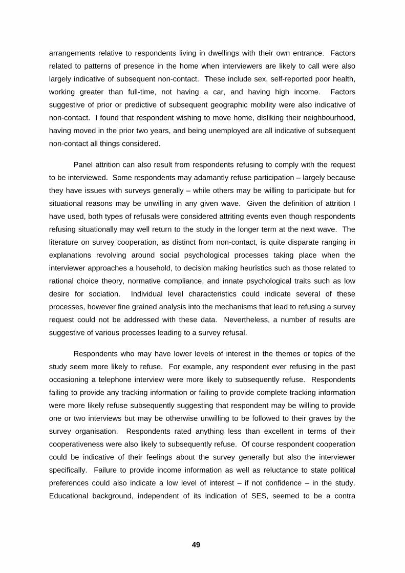
arrangements relative to respondents living in dwellings with their own entrance. Factors

related to patterns of presence in the home when interviewers are likely to call were also

largely indicative of subsequent non-contact. These include sex, self-reported poor health,

working greater than full-time, not having a car, and having high income. Factors

suggestive of prior or predictive of subsequent geographic mobility were also indicative of

non-contact. I found that respondent wishing to move home, disliking their neighbourhood,

having moved in the prior two years, and being unemployed are all indicative of subsequent

non-contact all things considered.

Panel attrition can also result from respondents refusing to comply with the request

to be interviewed. Some respondents may adamantly refuse participation – largely because

they have issues with surveys generally – while others may be willing to participate but for

situational reasons may be unwilling in any given wave. Given the definition of attrition I

have used, both types of refusals were considered attriting events even though respondents

refusing situationally may well return to the study in the longer term at the next wave. The

literature on survey cooperation, as distinct from non-contact, is quite disparate ranging in

explanations revolving around social psychological processes taking place when the

interviewer approaches a household, to decision making heuristics such as those related to

rational choice theory, normative compliance, and innate psychological traits such as low

desire for sociation. Individual level characteristics could indicate several of these

processes, however fine grained analysis into the mechanisms that lead to refusing a survey

request could not be addressed with these data. Nevertheless, a number of results are

suggestive of various processes leading to a survey refusal.

Respondents who may have lower levels of interest in the themes or topics of the

study seem more likely to refuse. For example, any respondent ever refusing in the past

occasioning a telephone interview were more likely to subsequently refuse. Respondents

failing to provide any tracking information or failing to provide complete tracking information

were more likely refuse subsequently suggesting that respondent may be willing to provide

one or two interviews but may be otherwise unwilling to be followed to their graves by the

survey organisation. Respondents rated anything less than excellent in terms of their

cooperativeness were also likely to subsequently refuse. Of course respondent cooperation

could be indicative of their feelings about the survey generally but also the interviewer

specifically. Failure to provide income information as well as reluctance to state political

preferences could also indicate a low level of interest – if not confidence – in the study.

Educational background, independent of its indication of SES, seemed to be a contra

49

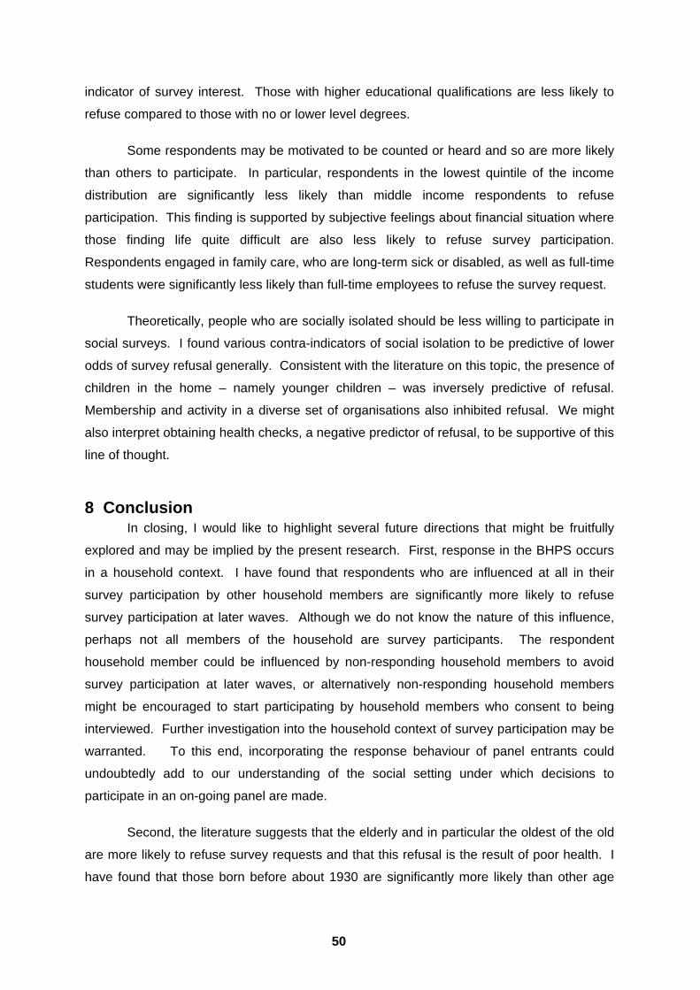
indicator of survey interest. Those with higher educational qualifications are less likely to

refuse compared to those with no or lower level degrees.

Some respondents may be motivated to be counted or heard and so are more likely

than others to participate. In particular, respondents in the lowest quintile of the income

distribution are significantly less likely than middle income respondents to refuse

participation. This finding is supported by subjective feelings about financial situation where

those finding life quite difficult are also less likely to refuse survey participation.

Respondents engaged in family care, who are long-term sick or disabled, as well as full-time

students were significantly less likely than full-time employees to refuse the survey request.

Theoretically, people who are socially isolated should be less willing to participate in

social surveys. I found various contra-indicators of social isolation to be predictive of lower

odds of survey refusal generally. Consistent with the literature on this topic, the presence of

children in the home – namely younger children – was inversely predictive of refusal.

Membership and activity in a diverse set of organisations also inhibited refusal. We might

also interpret obtaining health checks, a negative predictor of refusal, to be supportive of this

line of thought.

8 Conclusion In closing, I would like to highlight several future directions that might be fruitfully

explored and may be implied by the present research. First, response in the BHPS occurs

in a household context. I have found that respondents who are influenced at all in their

survey participation by other household members are significantly more likely to refuse

survey participation at later waves. Although we do not know the nature of this influence,

perhaps not all members of the household are survey participants. The respondent

household member could be influenced by non-responding household members to avoid

survey participation at later waves, or alternatively non-responding household members

might be encouraged to start participating by household members who consent to being

interviewed. Further investigation into the household context of survey participation may be

warranted. To this end, incorporating the response behaviour of panel entrants could

undoubtedly add to our understanding of the social setting under which decisions to

participate in an on-going panel are made.

Second, the literature suggests that the elderly and in particular the oldest of the old

are more likely to refuse survey requests and that this refusal is the result of poor health. I

have found that those born before about 1930 are significantly more likely than other age

50

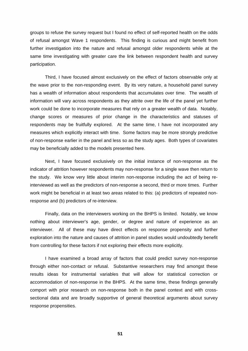
groups to refuse the survey request but I found no effect of self-reported health on the odds

of refusal amongst Wave 1 respondents. This finding is curious and might benefit from

further investigation into the nature and refusal amongst older respondents while at the

same time investigating with greater care the link between respondent health and survey

participation.

Third, I have focused almost exclusively on the effect of factors observable only at

the wave prior to the non-responding event. By its very nature, a household panel survey

has a wealth of information about respondents that accumulates over time. The wealth of

information will vary across respondents as they attrite over the life of the panel yet further

work could be done to incorporate measures that rely on a greater wealth of data. Notably,

change scores or measures of prior change in the characteristics and statuses of

respondents may be fruitfully explored. At the same time, I have not incorporated any

measures which explicitly interact with time. Some factors may be more strongly predictive

of non-response earlier in the panel and less so as the study ages. Both types of covariates

may be beneficially added to the models presented here.

Next, I have focused exclusively on the initial instance of non-response as the

indicator of attrition however respondents may non-response for a single wave then return to

the study. We know very little about interim non-response including the act of being re-

interviewed as well as the predictors of non-response a second, third or more times. Further

work might be beneficial in at least two areas related to this: (a) predictors of repeated non-

response and (b) predictors of re-interview.

Finally, data on the interviewers working on the BHPS is limited. Notably, we know

nothing about interviewer’s age, gender, or degree and nature of experience as an

interviewer. All of these may have direct effects on response propensity and further

exploration into the nature and causes of attrition in panel studies would undoubtedly benefit

from controlling for these factors if not exploring their effects more explicitly.

I have examined a broad array of factors that could predict survey non-response

through either non-contact or refusal. Substantive researchers may find amongst these

results ideas for instrumental variables that will allow for statistical correction or

accommodation of non-response in the BHPS. At the same time, these findings generally

comport with prior research on non-response both in the panel context and with cross-

sectional data and are broadly supportive of general theoretical arguments about survey

response propensities.

51

References Allen, K., Simpson, G., Winn, D. and Giovino, G. (1991) 'Response rates and

characteristics of adolescents in the 1989 Teenage Attitudes and Practices Survey', 1991 Proceedings of Survey Research Methods Section of the American Statistical Association, 575-580.

Allison, P. D. (1984) Event History Analysis: Regression for Longitudinal Event Data, Newbury Park, CA: Sage Publications, Inc.

Behr, A., Bellgardt, E. and Rendtel, U. (2005) 'Extent and Determinants of Panel Attrition in the European Community Household Panel', European Sociological Review, 21(5): 489-512.

Branden, L., Gritz, R. M. and Pergamit, M. R. (1995) 'The Effect of Interview Length on Attrition in the National Longitudinal Survey of Youth', No. NLS 95-28, US Department of Labour.

Brehm, J. (1993 ) The Phantom Respondents -- Opinion Surveys and Political Respresentation, Ann Arbor: University of Michigan Press.

Brown, P. R. and Bishop, G. F. (1982) 'Who Refuses and Resists in Telephone Surveys? Some New Evidence', in G. R.M. (ed), Univesrity of Cincinnati

Burton, J., Laurie, H. and Lynn, P. (2006) 'The long-term effectiveness of refusal conversion procedures on longitudinal surveys.' Journal of the Royal Statistical Society Series A -- Statistics in Society, 169: 459-478.

Campanelli, P. and O'Muircheartaigh, C. (1999) 'Interviewers, Interviewer Continuity, and Panel Survey Nonresponse', Quality and Quantity, 33: 59-76.

— (2002) 'The Importance of Experimental Control in Testing the Impact of Interviewer Continuity on Panel Survey Nonresponse', Quality and Quantity, 36: 129-144.

Campanelli, P., Sturgis, P. and Purdon, S. (1997) 'Can You Hear Me Knocking: An Investigation into the Impact of Interviewers on Survey Response Rates', London: Social and Community Planning Research.

Cannell, C. F., Groves, R. M., Magilavy, L., Mathiowetz, N. A. and Miller, P. V. (1987) 'An Experimental Comparison of Telephone and Personal Health Surveys', Statistics Technical Series 2, No. 106, National Center for Health.

Cheesbrough, S. (1993) 'Characteristics of Non-Responding Households in the Family Expenditure Survey', Survey Methodology Bulletin, 33: 12-18.

Couper, M. P. (1991) 'Modelling Survey Participation at the Interviewer Level in 1991', 1991 Proceedings of the Survey Research Methods Section of the American Statistical Association, 98-107. http://www.amstat.org/sections/srms/proceedings

52

DeMaio, T. J. (1985) 'Social Desirability and Survey Measurement: A Review', in C. Turner and E. Martin (eds) Surveying Subjective Phenomena, New York: Russell Sage Foundation & Basic Books.

Dillman, D. A. (2000) Mail and Internet Surveys: The Tailored Design Method, New York: John Wiley & Sons.

Dohrenwend, B. S. and Dohrenwend, B. P. (1968) 'Sources of Refusals in Surveys', Public Opinion Quarterly, 32(1): 74-83.

Dunkelberg, W. and Day, G. (1973) 'Nonresponse Bias and Callbacks in Sample Surveys', Journal of Marketing Research, 10: 160-168.

Fitzgerald, J., Gottschalk, P. and Moffitt, R. (1998) 'An Analysis of Sample Attrition in Panel Data: The Michigan Panel Study of Income Dynamics', The Journal of Human Resources, 33(2): 251-299.

Foster, K. (1998) 'Evaluating Nonresponse on Household Surveys', GSS Methodology Series, No. 8, London: Government Statistics Service.

Foster, K. and Bushnell, D. (1994) 'Nonresponse Bias on Government Surveys in Great Britain', Paper presented at The 5th International Workshop on Household Nonresponse, Ottawa, September 26-28.

Foster, K., Jackson, B., Thomas, M., Hunter, P. and Bennett, N. (1993) General Household Survey 1993, London: OPCS Social Survey Division.

Goyder, J. (1987) The Silent Minority -- Nonrespondents on Sample Surveys, Cambridge: Polity Press.

Groves, R. M. (1989) Survey Errors and Survey Costs, New York: John Wiley & Sons.

— (1990) 'Theories and Methods of Telephone Surveys', Annual Review of Sociology, 16: 221-240.

Groves, R. M. and Couper, M. P. (1998) Nonresponse in Household Interview Surveys, New York: John Wiley & Sons.

Groves, R. M., Dillman, D. A., Eltinge, J. L. and Little, R. J. A. (2002) Survey Nonresponse, New York: John Wiley & Sons.

Groves, R. M., Singer, E. and Corning, A. (2000) 'Leverage-Saliency Theory of Survey Participation', Public Opinion Quarterly, 64: 299-308.

Grusky, D. (2001) 'The Past, Present and Future of Social Inequality', in D. Grusky (ed) Social Stratification: Class, Race and Gender in Sociological Perspective, Oxford: Westview Press.

Hanushek, E. A. and Jackson, J. E. (1977) Statistical Methods for Social Scientists, Orlando, FL: Academic Press, Inc.

53

Hawkes, D. and Plewis, I. (2006) 'Modelling Nonresponse in the National Child Development Study', Journal of the Royal Statistical Society Series A, 169(3): 479-491.

Hawkins, D. F. (1975) 'Estimation of Nonresponse Bias', Sociological Methods and Research, 3: 461-488.

Heckman, J. J. and Singer, B. (1982) 'The identification problem in econometric models for duration data', in W. Hildebrand (ed) Advances in Econometrics, Cambridge: Cambridge University Press.

Iyer, R. (1984) 'NCDS Fourth Follow-up 1981: Analysis of Response', NCDS4 Working Paper, No. 25, London: National Children's Bureau. Http://www.cis.ioe.ac.uk/studies.asp?section=00010002000300070006

Jones, A. M., Koolman, X. and Rice, N. (2006) 'Health-related Non-response in the British Household Panel Survey and European Community Household Panel: Using Inverse-Probability-Weighted Estimators in Non-linear Models', Journal of the Royal Statistical Society Series A, 169(3): 543-569.

Kemsley, W. F. F. (1976) 'National Food Survey: A Study of Differential Response Based on a Comparison of the 1971 Sample with the Census', Statistical News, 35(18-22)

Kordos, J. (1994) 'Nonresponse Problems in Polish Household Surveys', Paper presented at The 5th International Workshop on Household Nonresponse, Ottawa, September 26-28.

Kreuter, F. and Valliant, R. (2007) 'A Survey on survey statistics: What is done and can be done in Stata', The Stata Journal, 7(1): 1-21.

Laurie, H., Smith, R. and Scott, L. (1999) 'Strategies for Reducing Nonresponse in a Longitudinal Panel Survey', Journal of Official Statistics, 15(2): 269-282.

Lepkowski, J. M. (1989) 'Treatment of Wave Nonresponse in Panel Surveys', in D. Kasprzyk, et al. (eds) Panel Surveys, New York: John Wiley & Sons.

Lepkowski, J. M. and Couper, M. P. (2002) 'Nonresponse in the Second Wave of Longitudinal Household Surveys', in R. M. Groves, et al. (eds) Survey Nonresponse, New York: John Wiley & Sons.

Lepkowski, J. M., Kalton, G. and Kasprzyk, D. (1989) 'Weighting Adjustments for Partial Nonresponse in the 1984 SIPP Panel' Survey of Income and Program Participation Selected Papers: The 1989 Meetings of the American Statistical Association, Washington, D.C.: U.S. Bureau of the Census.

Lillard, L. A. and Panis, C. W. A. (1998) 'Panel Attrition from the Panel Study of Income Dynamics', Journal of Political Economy, 94(3): 489-506.

Lindström, H. L. (1983) 'Non-Response Errors in Sample Surveys', Urval, No. 16, Orebro: Statistics Sweden.

54

Lyberg, I. and Lyberg, L. (1991) 'Nonresponse Research at Statistics Sweeden', 1991 Proceedings of the Survey Research Methods Section of the American Statistical Association, 78-87. http://www.amstat.org/sections/srms/proceedings

Lynn, P. (2003) 'PEDAKSI: Methodology for Collecting Data about Survey Non-Respondents', Quality and Quantity, 37(3): 239-261.

Lynn, P., Buck, N., Burton, J., Jäckle, A. and Laurie, H. (2005) 'A Review of Methodological Research Pertinent to Longitudinal Survey Design and Data Collection', ISER Working Papers, No. 2005-29, Colchester: University of Essex.

Lynn, P. and Clarke, P. (2002) 'Separating Refusal Bias and Non-Contact Bias: Evidence from UK National Surveys', Journal of the Royal Statistical Society Series D (The Statistician), 51(3): 319-333.

Lynn, P., Purdon, S., Hedges, B. and McAleese, I. (1994) 'The Youth Cohort Study: An Assessment of Altenative Weighting Strategies and Their Effects', Employment Department Research Series YCS Reports, No. 30, Sheffield: Employment Department.

Martin, E. (2007) 'Strength of Attachment: Survey Coverage of People with Tenuous ties to Residences', Demography, 44(2): 427-440.

Nathan, G. (1999) 'A Review of Sample Attrition and Representativeness in Three Longitudinal Surveys (The British Household Panel Survey, the 1970 British Cohort Study and The National Child Development Study)', Government Statistical Service Methodology Series, No. 13, London: GSS.

Nicoletti, C. and Peracchi, F. (2002) 'A Cross-Country Comparison of Survey Nonparticipation in the ECHP', ISER Working Papers, No. 2002-32, Colchester: University of Essex. Http://www.iser.essex.ac.uk/pubs/workpaps/pdf/2002-32.pdf

— (2005) 'Survey Response and Survey Characteristics: Microlevel Evidence from the European Community Household Panel', Journal of the Royal Statistical Society Series A, 168(4): 763-781.

O'Neil, M. J. (1979) 'Estimating the Nonresponse Bias Due to Refusals in Telephone Surveys', Public Opinion Quarterly, 43(2): 218-232.

Pannenberg, M. and Rendtel, U. (1996) 'Documentation of Sample Sizes and Panel Attrition on the German Socio-Economic Panel', Discussion Paper, No. 137, Berlin: DIW.

Robins, L. N. (1963) 'The Reluctant Respondent', Public Opinion Quarterly, 27(2): 276-286.

Ross, C. E. and Reynolds, J. R. (1996) 'The Effects of Power, Knowledge, and Trust on Income Disclosure in Surveys', Social Science Quarterly, 77(4): 899-911.

55

Smith, T. W. (1983) 'The Hidden 25 Percent: An Analysis of Nonresponse on the 1980 General Social Survey', Public Opinion Quarterly, 47: 386-404.

Stoop, I. A. L. (2005) The Hunt for the Last Respondent, The Hague, Netherlands: Social and Cultural Planning Office.

Taris, T. W. (2000) A Primer in Longitudinal Data Analysis, London: Sage.

Taylor, M. F., Brice, J., Buck, N. and Prentice-Lane, E. (2006) British Household Panel Survey User Manual Volume A: Introduction, Technical Report and Appendices., Colchester: University of Essex.

— (2007) 'The British Household Panel Study User Manual Volume A: Introduction, Technical Report and Appendices', Colchester: University of Essex. http://iserwww.essex.ac.uk/ulsc/bhps/doc/

Watson, D. (2003) 'Sample Attrition between Waves 1 and 5 in the European Community Household Panel', European Sociological Review, 19(4): 361-378.

Wilcox, J. B. (1977) 'The Interaction of Refusal and Not-at-Home Sources of Nonresponse Bias', Journal of Marketing Research, 14: 592-597.

Zabel, J. E. (1998) 'An Analysis of Attrition in the Panel Study of Income Dynamics and the Survey of Income and Program Participation with an Application to a Model of Labor Market Behavior', Journal of Human Resources, 33(2): 479-506.

56

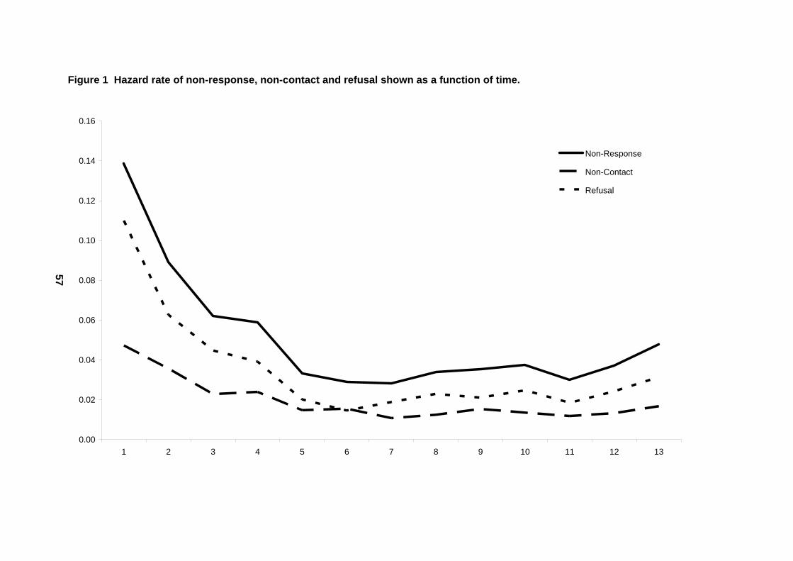
Figure 1 Hazard rate of non-response, non-contact and refusal shown as a function of time.

0.00

0.02

0.04

0.06

0.08

0.10

0.12

0.14

0.16

1 2 3 4 5 6 7 8 9 10 11 12 13

Non-Response

Non-Contact

Refusal

57

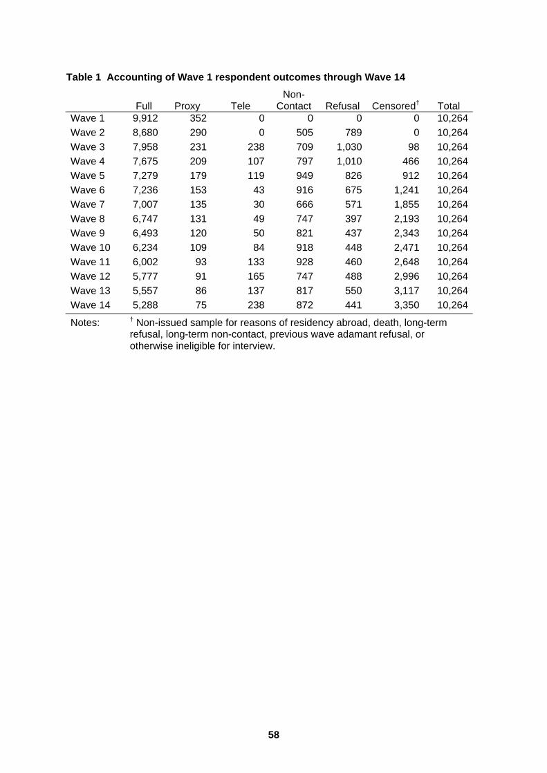
Table 1 Accounting of Wave 1 respondent outcomes through Wave 14

Full Proxy Tele Non-

Contact Refusal Censored† Total Wave 1 9,912 352 0 0 0 0 10,264Wave 2 8,680 290 0 505 789 0 10,264Wave 3 7,958 231 238 709 1,030 98 10,264Wave 4 7,675 209 107 797 1,010 466 10,264Wave 5 7,279 179 119 949 826 912 10,264Wave 6 7,236 153 43 916 675 1,241 10,264Wave 7 7,007 135 30 666 571 1,855 10,264Wave 8 6,747 131 49 747 397 2,193 10,264Wave 9 6,493 120 50 821 437 2,343 10,264Wave 10 6,234 109 84 918 448 2,471 10,264Wave 11 6,002 93 133 928 460 2,648 10,264Wave 12 5,777 91 165 747 488 2,996 10,264Wave 13 5,557 86 137 817 550 3,117 10,264Wave 14 5,288 75 238 872 441 3,350 10,264

Notes:

† Non-issued sample for reasons of residency abroad, death, long-term refusal, long-term non-contact, previous wave adamant refusal, or otherwise ineligible for interview.

58

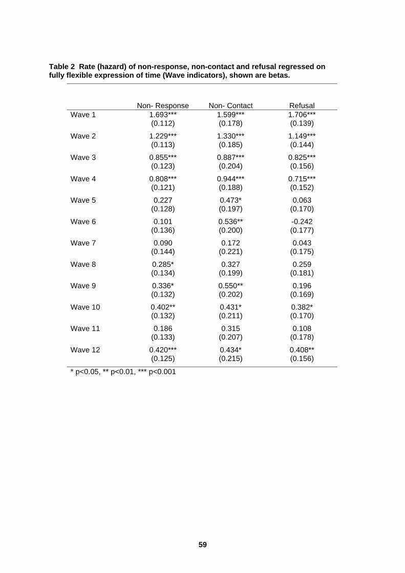
Table 2 Rate (hazard) of non-response, non-contact and refusal regressed on fully flexible expression of time (Wave indicators), shown are betas.

Non- Response Non- Contact Refusal Wave 1 1.693*** 1.599*** 1.706*** (0.112) (0.178) (0.139)

Wave 2 1.229*** 1.330*** 1.149*** (0.113) (0.185) (0.144)

Wave 3 0.855*** 0.887*** 0.825*** (0.123) (0.204) (0.156)

Wave 4 0.808*** 0.944*** 0.715*** (0.121) (0.188) (0.152)

Wave 5 0.227 0.473* 0.063 (0.128) (0.197) (0.170)

Wave 6 0.101 0.536** -0.242 (0.136) (0.200) (0.177)

Wave 7 0.090 0.172 0.043 (0.144) (0.221) (0.175)

Wave 8 0.285* 0.327 0.259 (0.134) (0.199) (0.181)

Wave 9 0.336* 0.550** 0.196 (0.132) (0.202) (0.169)

Wave 10 0.402** 0.431* 0.382* (0.132) (0.211) (0.170)

Wave 11 0.186 0.315 0.108 (0.133) (0.207) (0.178)

Wave 12 0.420*** 0.434* 0.408** (0.125) (0.215) (0.156)

* p<0.05, ** p<0.01, *** p<0.001

59

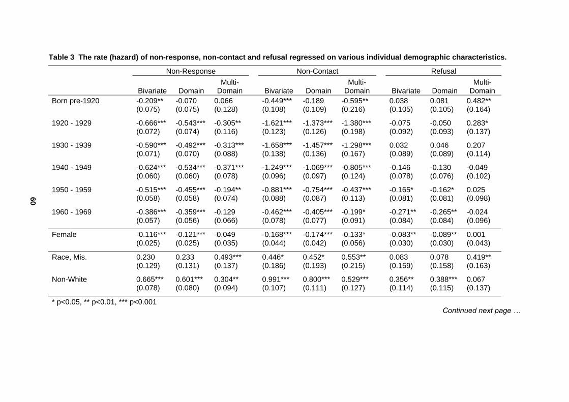
Table 3 The rate (hazard) of non-response, non-contact and refusal regressed on various individual demographic characteristics.

Non-Response Non-Contact Refusal

Bivariate Domain Multi-

Domain Bivariate Domain Multi-

Domain Bivariate Domain Multi-

Domain Born pre-1920 -0.209** -0.070 0.066 -0.449*** -0.189 -0.595** 0.038 0.081 0.482** (0.075) (0.075) (0.128) (0.108) (0.109) (0.216) (0.105) (0.105) (0.164)

1920 - 1929 -0.666*** -0.543*** -0.305** -1.621*** -1.373*** -1.380*** -0.075 -0.050 0.283* (0.072) (0.074) (0.116) (0.123) (0.126) (0.198) (0.092) (0.093) (0.137)

1930 - 1939 -0.590*** -0.492*** -0.313*** -1.658*** -1.457*** -1.298*** 0.032 0.046 0.207 (0.071) (0.070) (0.088) (0.138) (0.136) (0.167) (0.089) (0.089) (0.114)

1940 - 1949 -0.624*** -0.534*** -0.371*** -1.249*** -1.069*** -0.805*** -0.146 -0.130 -0.049 (0.060) (0.060) (0.078) (0.096) (0.097) (0.124) (0.078) (0.076) (0.102)

1950 - 1959 -0.515*** -0.455*** -0.194** -0.881*** -0.754*** -0.437*** -0.165* -0.162* 0.025 (0.058) (0.058) (0.074) (0.088) (0.087) (0.113) (0.081) (0.081) (0.098)

1960 - 1969 -0.386*** -0.359*** -0.129 -0.462*** -0.405*** -0.199* -0.271** -0.265** -0.024 (0.057) (0.056) (0.066) (0.078) (0.077) (0.091) (0.084) (0.084) (0.096)

Female -0.116*** -0.121*** -0.049 -0.168*** -0.174*** -0.133* -0.083** -0.089** 0.001 (0.025) (0.025) (0.035) (0.044) (0.042) (0.056) (0.030) (0.030) (0.043)

Race, Mis. 0.230 0.233 0.493*** 0.446* 0.452* 0.553** 0.083 0.078 0.419** (0.129) (0.131) (0.137) (0.186) (0.193) (0.215) (0.159) (0.158) (0.163)

Non-White 0.665*** 0.601*** 0.304** 0.991*** 0.800*** 0.529*** 0.356** 0.388*** 0.067 (0.078) (0.080) (0.094) (0.107) (0.111) (0.127) (0.114) (0.115) (0.137)

* p<0.05, ** p<0.01, *** p<0.001

60

Continued next page …

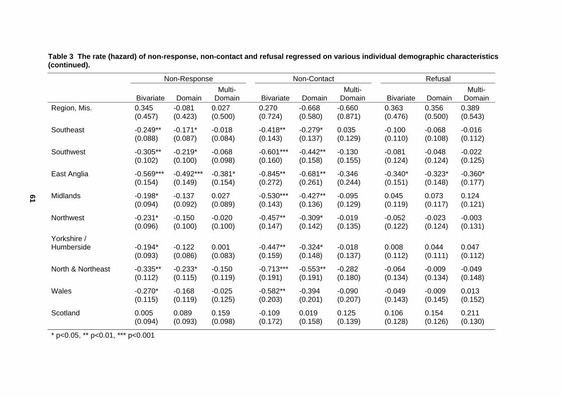
Table 3 The rate (hazard) of non-response, non-contact and refusal regressed on various individual demographic characteristics (continued).

Non-Response Non-Contact Refusal

Bivariate Domain Multi-

Domain Bivariate Domain Multi-

Domain Bivariate Domain Multi-

Domain Region, Mis. 0.345 -0.081 0.027 0.270 -0.668 -0.660 0.363 0.356 0.389 (0.457) (0.423) (0.500) (0.724) (0.580) (0.871) (0.476) (0.500) (0.543)

Southeast -0.249** -0.171* -0.018 -0.418** -0.279* 0.035 -0.100 -0.068 -0.016 (0.088) (0.087) (0.084) (0.143) (0.137) (0.129) (0.110) (0.108) (0.112)

Southwest -0.305** -0.219* -0.068 -0.601*** -0.442** -0.130 -0.081 -0.048 -0.022 (0.102) (0.100) (0.098) (0.160) (0.158) (0.155) (0.124) (0.124) (0.125)

East Anglia -0.569*** -0.492*** -0.381* -0.845** -0.681** -0.346 -0.340* -0.323* -0.360* (0.154) (0.149) (0.154) (0.272) (0.261) (0.244) (0.151) (0.148) (0.177)

Midlands -0.198* -0.137 0.027 -0.530*** -0.427** -0.095 0.045 0.073 0.124 (0.094) (0.092) (0.089) (0.143) (0.136) (0.129) (0.119) (0.117) (0.121)

Northwest -0.231* -0.150 -0.020 -0.457** -0.309* -0.019 -0.052 -0.023 -0.003 (0.096) (0.100) (0.100) (0.147) (0.142) (0.135) (0.122) (0.124) (0.131)

Yorkshire / Humberside -0.194* -0.122 0.001 -0.447** -0.324* -0.018 0.008 0.044 0.047 (0.093) (0.086) (0.083) (0.159) (0.148) (0.137) (0.112) (0.111) (0.112)

North & Northeast -0.335** -0.233* -0.150 -0.713*** -0.553** -0.282 -0.064 -0.009 -0.049 (0.112) (0.115) (0.119) (0.191) (0.191) (0.180) (0.134) (0.134) (0.148)

Wales -0.270* -0.168 -0.025 -0.582** -0.394 -0.090 -0.049 -0.009 0.013 (0.115) (0.119) (0.125) (0.203) (0.201) (0.207) (0.143) (0.145) (0.152)

Scotland 0.005 0.089 0.159 -0.109 0.019 0.125 0.106 0.154 0.211 (0.094) (0.093) (0.098) (0.172) (0.158) (0.139) (0.128) (0.126) (0.130)

* p<0.05, ** p<0.01, *** p<0.001

61

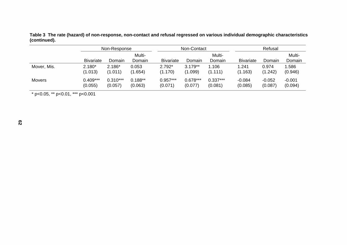
Table 3 The rate (hazard) of non-response, non-contact and refusal regressed on various individual demographic characteristics (continued).

Non-Response Non-Contact Refusal

Bivariate Domain Multi-

Domain Bivariate Domain Multi-

Domain Bivariate Domain Multi-

Domain Mover, Mis. 2.180* 2.186* 0.053 2.792* 3.179** 1.106 1.241 0.974 1.586 (1.013) (1.011) (1.654) (1.170) (1.099) (1.111) (1.163) (1.242) (0.946)

Movers 0.409*** 0.310*** 0.188** 0.957*** 0.678*** 0.337*** -0.084 -0.052 -0.001 (0.055) (0.057) (0.063) (0.071) (0.077) (0.081) (0.085) (0.087) (0.094)

* p<0.05, ** p<0.01, *** p<0.001

62

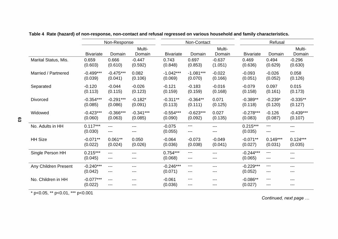
Table 4 Rate (hazard) of non-response, non-contact and refusal regressed on various household and family characteristics.

Non-Response Non-Contact Refusal

Bivariate Domain Multi-

Domain Bivariate Domain Multi-

Domain Bivariate Domain Multi-

Domain Marital Status, Mis. 0.659 0.666 -0.447 0.743 0.697 -0.637 0.469 0.494 -0.296 (0.603) (0.610) (0.592) (0.848) (0.853) (1.051) (0.636) (0.629) (0.630)

Married / Partnered -0.499*** -0.475*** 0.082 -1.042*** -1.081*** -0.022 -0.093 -0.026 0.058 (0.039) (0.041) (0.106) (0.069) (0.070) (0.166) (0.051) (0.052) (0.126)

Separated -0.120 -0.044 -0.026 -0.121 -0.183 -0.016 -0.079 0.097 0.015 (0.113) (0.115) (0.123) (0.159) (0.159) (0.168) (0.158) (0.161) (0.173)

Divorced -0.354*** -0.291*** -0.182* -0.311** -0.364** 0.071 -0.389** -0.239* -0.335** (0.085) (0.086) (0.091) (0.113) (0.111) (0.125) (0.118) (0.120) (0.127)

Widowed -0.423*** -0.366*** -0.341*** -0.554*** -0.623*** 0.027 -0.278*** -0.126 -0.439*** (0.060) (0.063) (0.085) (0.090) (0.092) (0.135) (0.083) (0.087) (0.107)

No. Adults in HH 0.117*** --- --- -0.075 --- --- 0.215*** --- --- (0.030) --- --- (0.055) --- --- (0.035) --- ---

HH Size -0.071** 0.061** 0.050 -0.064 -0.073 -0.049 -0.071** 0.149*** 0.124*** (0.022) (0.024) (0.026) (0.036) (0.038) (0.041) (0.027) (0.031) (0.035)

Single Person HH 0.215*** --- --- 0.754*** --- --- -0.244*** --- --- (0.045) --- --- (0.068) --- --- (0.065) --- ---

Any Children Present -0.240*** --- --- -0.246*** --- --- -0.229*** --- --- (0.042) --- --- (0.071) --- --- (0.052) --- ---

No. Children in HH -0.077*** --- --- -0.061 --- --- -0.086** --- --- (0.022) --- --- (0.036) --- --- (0.027) --- ---

* p<0.05, ** p<0.01, *** p<0.001

63

Continued, next page …

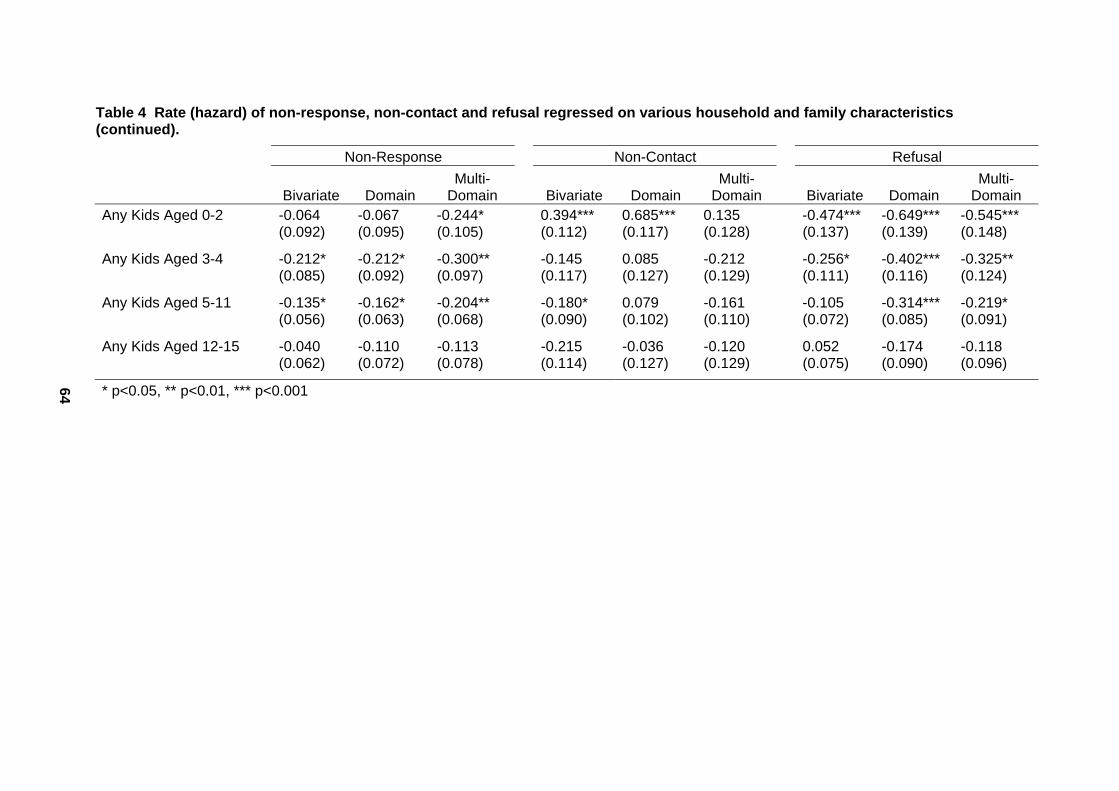
Table 4 Rate (hazard) of non-response, non-contact and refusal regressed on various household and family characteristics (continued).

Non-Response Non-Contact Refusal

Bivariate Domain Multi-

Domain Bivariate Domain Multi-

Domain Bivariate Domain Multi-

Domain Any Kids Aged 0-2 -0.064 -0.067 -0.244* 0.394*** 0.685*** 0.135 -0.474*** -0.649*** -0.545*** (0.092) (0.095) (0.105) (0.112) (0.117) (0.128) (0.137) (0.139) (0.148)

Any Kids Aged 3-4 -0.212* -0.212* -0.300** -0.145 0.085 -0.212 -0.256* -0.402*** -0.325** (0.085) (0.092) (0.097) (0.117) (0.127) (0.129) (0.111) (0.116) (0.124)

Any Kids Aged 5-11 -0.135* -0.162* -0.204** -0.180* 0.079 -0.161 -0.105 -0.314*** -0.219* (0.056) (0.063) (0.068) (0.090) (0.102) (0.110) (0.072) (0.085) (0.091)

Any Kids Aged 12-15 -0.040 -0.110 -0.113 -0.215 -0.036 -0.120 0.052 -0.174 -0.118 (0.062) (0.072) (0.078) (0.114) (0.127) (0.129) (0.075) (0.090) (0.096)

* p<0.05, ** p<0.01, *** p<0.001 64

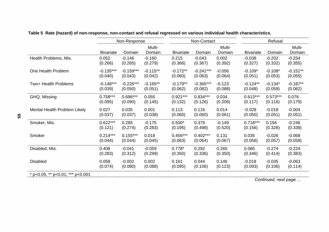
Table 5 Rate (hazard) of non-response, non-contact and refusal regressed on various individual health characteristics.

Non-Response Non-Contact Refusal

Bivariate Domain Multi-

Domain Bivariate Domain Multi-

Domain Bivariate Domain Multi-

Domain Health Problems, Mis. 0.052 -0.146 -0.160 0.215 -0.043 0.002 -0.038 -0.202 -0.254 (0.266) (0.265) (0.279) (0.366) (0.367) (0.392) (0.327) (0.332) (0.355)

One Health Problem -0.135*** -0.159*** -0.115** -0.172** -0.241*** -0.056 -0.109* -0.108* -0.151** (0.040) (0.043) (0.042) (0.060) (0.063) (0.064) (0.051) (0.053) (0.055)

Two+ Health Problems -0.148*** -0.226*** -0.165** -0.179** -0.365*** -0.123 -0.124** -0.134* -0.187** (0.039) (0.050) (0.051) (0.062) (0.082) (0.088) (0.048) (0.059) (0.062)

GHQ, Missing 0.758*** 0.696*** 0.055 0.921*** 0.834*** 0.034 0.613*** 0.573*** 0.076 (0.095) (0.090) (0.145) (0.132) (0.126) (0.206) (0.117) (0.116) (0.179)

Mental Health Problem Likely 0.027 0.035 0.001 0.113 0.116 0.014 -0.028 -0.018 -0.004 (0.037) (0.037) (0.038) (0.060) (0.060) (0.061) (0.050) (0.051) (0.051)

Smoker, Mis. 0.622*** 0.285 -0.175 0.500* 0.379 -0.149 0.718*** 0.194 -0.246 (0.121) (0.274) (0.283) (0.195) (0.498) (0.520) (0.156) (0.328) (0.338)

Smoker 0.214*** 0.155*** 0.018 0.456*** 0.402*** 0.131 0.035 -0.026 -0.068 (0.044) (0.044) (0.045) (0.063) (0.064) (0.067) (0.056) (0.057) (0.058)

Disabled, Mis. 0.408 -0.041 -0.059 0.778* 0.292 0.265 0.085 -0.274 -0.224 (0.283) (0.312) (0.299) (0.350) (0.336) (0.350) (0.346) (0.414) (0.383)

Disabled 0.058 -0.002 0.002 0.161 0.044 0.146 -0.018 -0.035 -0.063 (0.074) (0.080) (0.088) (0.095) (0.106) (0.123) (0.093) (0.106) (0.114)

* p<0.05, ** p<0.01, *** p<0.001

65

Continued, next page …

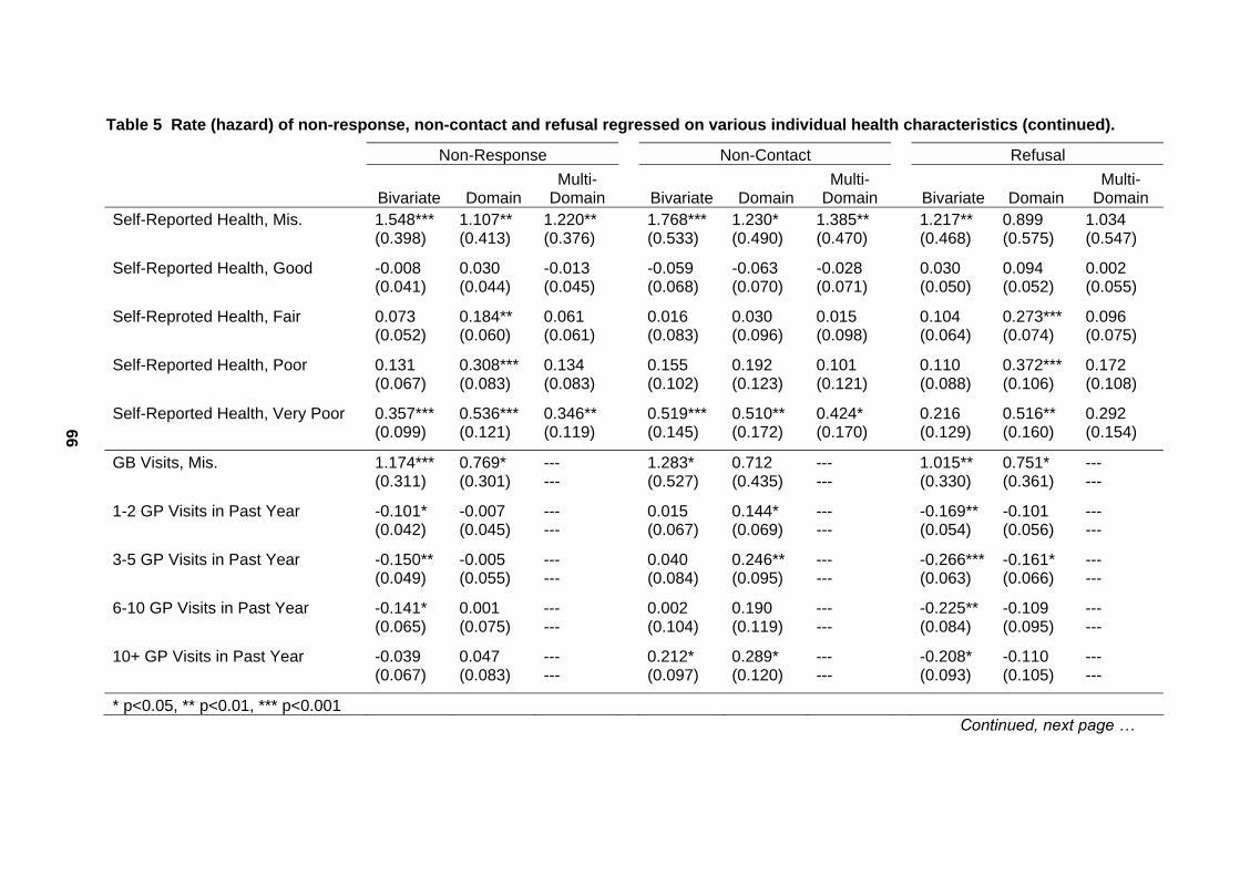
Table 5 Rate (hazard) of non-response, non-contact and refusal regressed on various individual health characteristics (continued).

Non-Response Non-Contact Refusal

Bivariate Domain Multi-

Domain Bivariate Domain Multi-

Domain Bivariate Domain Multi-

Domain Self-Reported Health, Mis. 1.548*** 1.107** 1.220** 1.768*** 1.230* 1.385** 1.217** 0.899 1.034 (0.398) (0.413) (0.376) (0.533) (0.490) (0.470) (0.468) (0.575) (0.547)

Self-Reported Health, Good -0.008 0.030 -0.013 -0.059 -0.063 -0.028 0.030 0.094 0.002 (0.041) (0.044) (0.045) (0.068) (0.070) (0.071) (0.050) (0.052) (0.055)

Self-Reproted Health, Fair 0.073 0.184** 0.061 0.016 0.030 0.015 0.104 0.273*** 0.096 (0.052) (0.060) (0.061) (0.083) (0.096) (0.098) (0.064) (0.074) (0.075)

Self-Reported Health, Poor 0.131 0.308*** 0.134 0.155 0.192 0.101 0.110 0.372*** 0.172 (0.067) (0.083) (0.083) (0.102) (0.123) (0.121) (0.088) (0.106) (0.108)

Self-Reported Health, Very Poor 0.357*** 0.536*** 0.346** 0.519*** 0.510** 0.424* 0.216 0.516** 0.292 (0.099) (0.121) (0.119) (0.145) (0.172) (0.170) (0.129) (0.160) (0.154)

GB Visits, Mis. 1.174*** 0.769* --- 1.283* 0.712 --- 1.015** 0.751* --- (0.311) (0.301) --- (0.527) (0.435) --- (0.330) (0.361) ---

1-2 GP Visits in Past Year -0.101* -0.007 --- 0.015 0.144* --- -0.169** -0.101 --- (0.042) (0.045) --- (0.067) (0.069) --- (0.054) (0.056) ---

3-5 GP Visits in Past Year -0.150** -0.005 --- 0.040 0.246** --- -0.266*** -0.161* --- (0.049) (0.055) --- (0.084) (0.095) --- (0.063) (0.066) ---

6-10 GP Visits in Past Year -0.141* 0.001 --- 0.002 0.190 --- -0.225** -0.109 --- (0.065) (0.075) --- (0.104) (0.119) --- (0.084) (0.095) ---

10+ GP Visits in Past Year -0.039 0.047 --- 0.212* 0.289* --- -0.208* -0.110 --- (0.067) (0.083) --- (0.097) (0.120) --- (0.093) (0.105) ---

* p<0.05, ** p<0.01, *** p<0.001

66

Continued, next page …

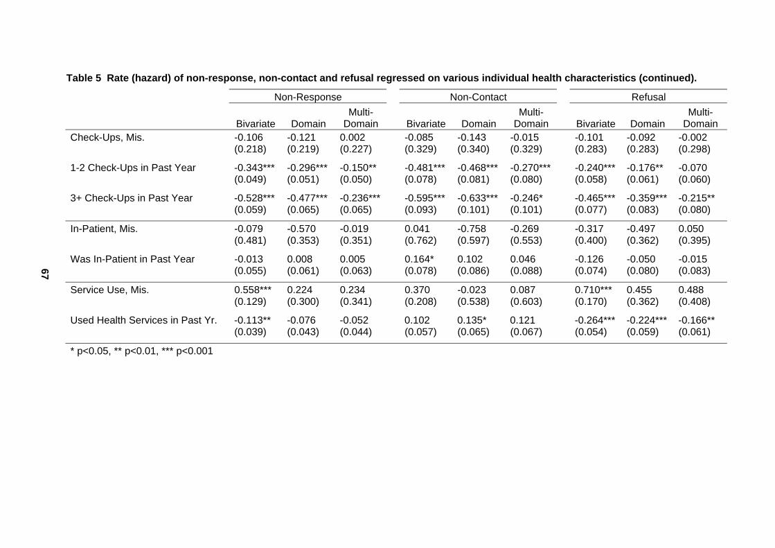
Table 5 Rate (hazard) of non-response, non-contact and refusal regressed on various individual health characteristics (continued).

Non-Response Non-Contact Refusal

Bivariate Domain Multi-

Domain Bivariate Domain Multi-

Domain Bivariate Domain Multi-

Domain Check-Ups, Mis. -0.106 -0.121 0.002 -0.085 -0.143 -0.015 -0.101 -0.092 -0.002 (0.218) (0.219) (0.227) (0.329) (0.340) (0.329) (0.283) (0.283) (0.298)

1-2 Check-Ups in Past Year -0.343*** -0.296*** -0.150** -0.481*** -0.468*** -0.270*** -0.240*** -0.176** -0.070 (0.049) (0.051) (0.050) (0.078) (0.081) (0.080) (0.058) (0.061) (0.060)

3+ Check-Ups in Past Year -0.528*** -0.477*** -0.236*** -0.595*** -0.633*** -0.246* -0.465*** -0.359*** -0.215** (0.059) (0.065) (0.065) (0.093) (0.101) (0.101) (0.077) (0.083) (0.080)

In-Patient, Mis. -0.079 -0.570 -0.019 0.041 -0.758 -0.269 -0.317 -0.497 0.050 (0.481) (0.353) (0.351) (0.762) (0.597) (0.553) (0.400) (0.362) (0.395)

Was In-Patient in Past Year -0.013 0.008 0.005 0.164* 0.102 0.046 -0.126 -0.050 -0.015 (0.055) (0.061) (0.063) (0.078) (0.086) (0.088) (0.074) (0.080) (0.083)

Service Use, Mis. 0.558*** 0.224 0.234 0.370 -0.023 0.087 0.710*** 0.455 0.488 (0.129) (0.300) (0.341) (0.208) (0.538) (0.603) (0.170) (0.362) (0.408)

Used Health Services in Past Yr. -0.113** -0.076 -0.052 0.102 0.135* 0.121 -0.264*** -0.224*** -0.166** (0.039) (0.043) (0.044) (0.057) (0.065) (0.067) (0.054) (0.059) (0.061)

* p<0.05, ** p<0.01, *** p<0.001

67

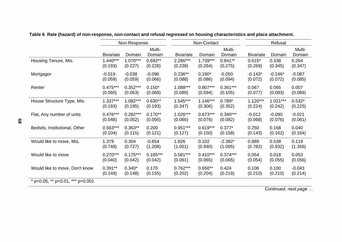
Table 6 Rate (hazard) of non-response, non-contact and refusal regressed on housing characteristics and place attachment.

Non-Response Non-Contact Refusal

BivariateMulti-

Domain Bivariate Domain Multi-

Domain Domain Bivariate Domain Multi-

Domain Housing Tenure, Mis. 1.440*** 1.070*** 0.692** 2.286*** 1.739*** 0.841** 0.615* 0.338 0.264 (0.193) (0.227) (0.228) (0.238) (0.264) (0.275) (0.269) (0.345) (0.347)

Mortgagor -0.019 -0.038 -0.096 0.236** 0.190* -0.050 -0.143* -0.146* -0.087 (0.059) (0.059) (0.066) (0.088) (0.086) (0.094) (0.072) (0.072) (0.085)

Renter 0.475*** 0.352*** 0.150* 1.088*** 0.807*** 0.361*** 0.067 0.065 0.007 (0.060) (0.063) (0.068) (0.089) (0.094) (0.105) (0.077) (0.083) (0.089)

House Structure Type, Mis. 1.337*** 1.082*** 0.630** 1.545*** 1.146*** 0.789* 1.120*** 1.021*** 0.532* (0.193) (0.195) (0.193) (0.347) (0.306) (0.352) (0.224) (0.242) (0.225)

Flat, Any number of units 0.476*** 0.282*** 0.170** 1.026*** 0.673*** 0.340*** -0.012 -0.090 -0.021 (0.048) (0.052) (0.056) (0.066) (0.076) (0.082) (0.068) (0.076) (0.081)

Bedsits, Institutional, Other 0.563*** 0.363** 0.200 0.951*** 0.619*** 0.377* 0.250 0.168 0.040 (0.104) (0.115) (0.121) (0.127) (0.150) (0.158) (0.143) (0.162) (0.164)

Would like to move, Mis. 1.379 0.304 -0.654 1.826 0.102 -2.382* 0.889 0.538 0.119 (0.748) (0.727) (1.208) (1.051) (0.940) (1.095) (0.782) (0.932) (1.356)

Would like to move 0.270*** 0.175*** 0.185*** 0.581*** 0.410*** 0.374*** 0.054 0.018 0.053 (0.040) (0.042) (0.042) (0.061) (0.065) (0.065) (0.054) (0.055) (0.056)

Would like to move, Don't know 0.391** 0.340* 0.170 0.762*** 0.650** 0.424 0.106 0.100 -0.043 (0.149) (0.148) (0.155) (0.202) (0.204) (0.219) (0.210) (0.210) (0.214)

* p<0.05, ** p<0.01, *** p<0.001

68

Continued, next page …

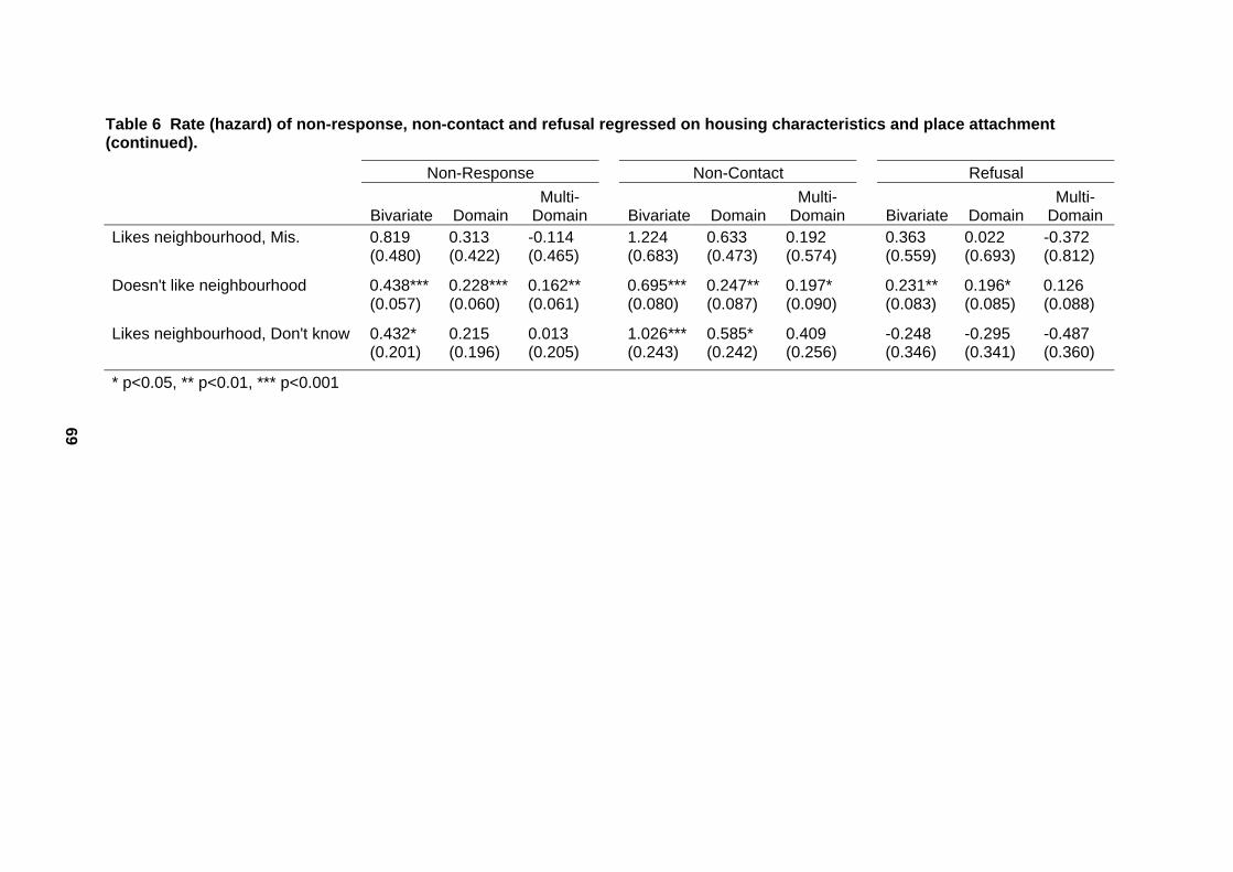
Table 6 Rate (hazard) of non-response, non-contact and refusal regressed on housing characteristics and place attachment (continued).

Non-Response Non-Contact Refusal

Bivariate Domain Multi-

Domain Bivariate Domain Multi-

Domain Bivariate Domain Multi-

Domain Likes neighbourhood, Mis. 0.819 0.313 -0.114 1.224 0.633 0.192 0.363 0.022 -0.372 (0.480) (0.422) (0.465) (0.683) (0.473) (0.574) (0.559) (0.693) (0.812)

Doesn't like neighbourhood 0.438*** 0.228*** 0.162** 0.695*** 0.247** 0.197* 0.231** 0.196* 0.126 (0.057) (0.060) (0.061) (0.080) (0.087) (0.090) (0.083) (0.085) (0.088)

Likes neighbourhood, Don't know 0.432* 0.215 0.013 1.026*** 0.585* 0.409 -0.248 -0.295 -0.487 (0.201) (0.196) (0.205) (0.243) (0.242) (0.256) (0.346) (0.341) (0.360)

* p<0.05, ** p<0.01, *** p<0.001

69

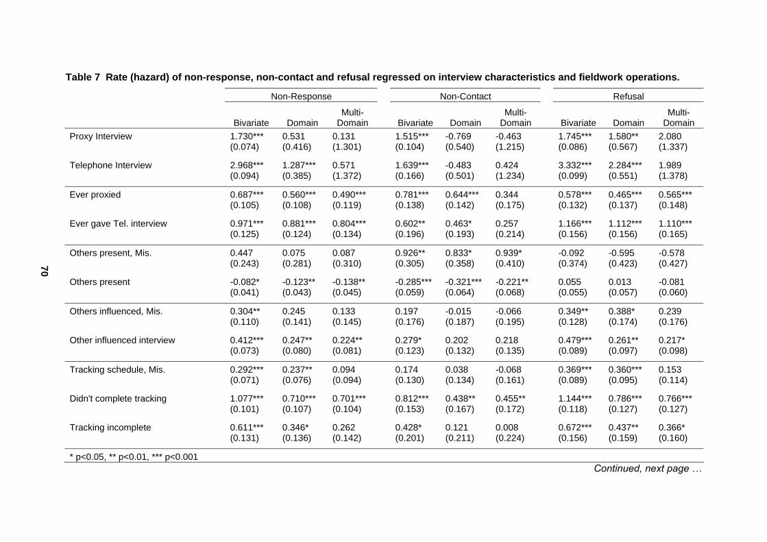
Table 7 Rate (hazard) of non-response, non-contact and refusal regressed on interview characteristics and fieldwork operations.

Non-Response Non-Contact Refusal

Bivariate Domain Multi-

Domain Bivariate Domain Multi-

Domain Bivariate Domain Multi-

Domain Proxy Interview 1.730*** 0.531 0.131 1.515*** -0.769 -0.463 1.745*** 1.580** 2.080 (0.074) (0.416) (1.301) (0.104) (0.540) (1.215) (0.086) (0.567) (1.337)

Telephone Interview 2.968*** 1.287*** 0.571 1.639*** -0.483 0.424 3.332*** 2.284*** 1.989 (0.094) (0.385) (1.372) (0.166) (0.501) (1.234) (0.099) (0.551) (1.378)

Ever proxied 0.687*** 0.560*** 0.490*** 0.781*** 0.644*** 0.344 0.578*** 0.465*** 0.565*** (0.105) (0.108) (0.119) (0.138) (0.142) (0.175) (0.132) (0.137) (0.148)

Ever gave Tel. interview 0.971*** 0.881*** 0.804*** 0.602** 0.463* 0.257 1.166*** 1.112*** 1.110*** (0.125) (0.124) (0.134) (0.196) (0.193) (0.214) (0.156) (0.156) (0.165)

Others present, Mis. 0.447 0.075 0.087 0.926** 0.833* 0.939* -0.092 -0.595 -0.578 (0.243) (0.281) (0.310) (0.305) (0.358) (0.410) (0.374) (0.423) (0.427)

Others present -0.082* -0.123** -0.138** -0.285*** -0.321*** -0.221** 0.055 0.013 -0.081 (0.041) (0.043) (0.045) (0.059) (0.064) (0.068) (0.055) (0.057) (0.060)

Others influenced, Mis. 0.304** 0.245 0.133 0.197 -0.015 -0.066 0.349** 0.388* 0.239 (0.110) (0.141) (0.145) (0.176) (0.187) (0.195) (0.128) (0.174) (0.176)

Other influenced interview 0.412*** 0.247** 0.224** 0.279* 0.202 0.218 0.479*** 0.261** 0.217* (0.073) (0.080) (0.081) (0.123) (0.132) (0.135) (0.089) (0.097) (0.098)

Tracking schedule, Mis. 0.292*** 0.237** 0.094 0.174 0.038 -0.068 0.369*** 0.360*** 0.153 (0.071) (0.076) (0.094) (0.130) (0.134) (0.161) (0.089) (0.095) (0.114)

Didn't complete tracking 1.077*** 0.710*** 0.701*** 0.812*** 0.438** 0.455** 1.144*** 0.786*** 0.766*** (0.101) (0.107) (0.104) (0.153) (0.167) (0.172) (0.118) (0.127) (0.127)

Tracking incomplete 0.611*** 0.346* 0.262 0.428* 0.121 0.008 0.672*** 0.437** 0.366* (0.131) (0.136) (0.142) (0.201) (0.211) (0.224) (0.156) (0.159) (0.160)

* p<0.05, ** p<0.01, *** p<0.001

70

Continued, next page …

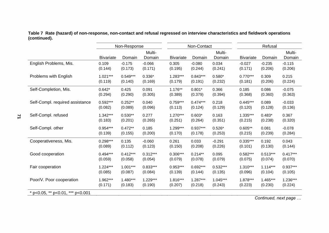
Table 7 Rate (hazard) of non-response, non-contact and refusal regressed on interview characteristics and fieldwork operations (continued).

Non-Response Non-Contact Refusal

Bivariate Domain Multi-

Domain Bivariate Domain Multi-

Domain Bivariate Domain Multi-

Domain English Problems, Mis. 0.109 -0.175 -0.066 0.305 -0.080 0.034 -0.027 -0.235 -0.115 (0.144) (0.173) (0.171) (0.195) (0.244) (0.241) (0.171) (0.206) (0.206)

Problems with English 1.021*** 0.549*** 0.336* 1.283*** 0.843*** 0.580* 0.770*** 0.309 0.215 (0.119) (0.140) (0.169) (0.179) (0.191) (0.232) (0.181) (0.206) (0.224)

Self-Completion, Mis. 0.642* 0.425 0.091 1.176** 0.801* 0.366 0.185 0.086 -0.075 (0.294) (0.290) (0.305) (0.389) (0.379) (0.394) (0.368) (0.360) (0.363)

Self-Compl. required assistance 0.592*** 0.252** 0.040 0.759*** 0.474*** 0.218 0.445*** 0.089 -0.033 (0.082) (0.089) (0.096) (0.113) (0.124) (0.129) (0.120) (0.128) (0.136)

Self-Compl. refused 1.342*** 0.530** 0.277 1.270*** 0.603* 0.163 1.335*** 0.483* 0.367 (0.183) (0.201) (0.265) (0.251) (0.264) (0.351) (0.215) (0.238) (0.320)

Self-Compl. other 0.954*** 0.472** 0.185 1.299*** 0.937*** 0.526* 0.605** 0.081 -0.078 (0.139) (0.155) (0.200) (0.170) (0.178) (0.253) (0.215) (0.239) (0.284)

Cooperativeness, Mis. 0.298*** 0.135 -0.060 0.261 0.033 -0.291 0.335*** 0.192 0.043 (0.089) (0.112) (0.123) (0.150) (0.208) (0.226) (0.101) (0.130) (0.144)

Good cooperation 0.494*** 0.412*** 0.312*** 0.306*** 0.214** 0.095 0.582*** 0.513*** 0.417*** (0.059) (0.058) (0.054) (0.079) (0.078) (0.079) (0.075) (0.074) (0.070)

Fair cooperation 1.224*** 1.001*** 0.833*** 0.953*** 0.692*** 0.532*** 1.310*** 1.114*** 0.937*** (0.085) (0.087) (0.084) (0.139) (0.144) (0.135) (0.096) (0.104) (0.105)

Poor/V. Poor cooperation 1.962*** 1.480*** 1.229*** 1.816*** 1.287*** 1.045*** 1.878*** 1.465*** 1.236*** (0.171) (0.183) (0.190) (0.207) (0.218) (0.243) (0.223) (0.230) (0.224)

* p<0.05, ** p<0.01, *** p<0.001

71

Continued, next page …

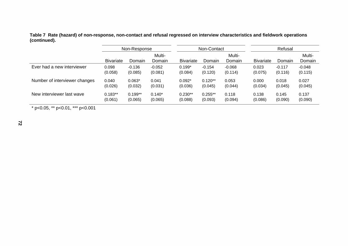
Table 7 Rate (hazard) of non-response, non-contact and refusal regressed on interview characteristics and fieldwork operations (continued).

Non-Response Non-Contact Refusal

Bivariate Domain Multi-

Domain Bivariate Domain Multi-

Domain Bivariate Domain Multi-

Domain Ever had a new interviewer 0.098 -0.136 -0.052 0.199* -0.154 -0.068 0.023 -0.117 -0.048 (0.058) (0.085) (0.081) (0.084) (0.120) (0.114) (0.075) (0.116) (0.115)

Number of interviewer changes 0.040 0.063* 0.041 0.092* 0.120** 0.053 0.000 0.018 0.027 (0.026) (0.032) (0.031) (0.036) (0.045) (0.044) (0.034) (0.045) (0.045)

New interviewer last wave 0.183** 0.199** 0.140* 0.230** 0.255** 0.118 0.138 0.145 0.137 (0.061) (0.065) (0.065) (0.088) (0.093) (0.094) (0.086) (0.090) (0.090)

* p<0.05, ** p<0.01, *** p<0.001

72

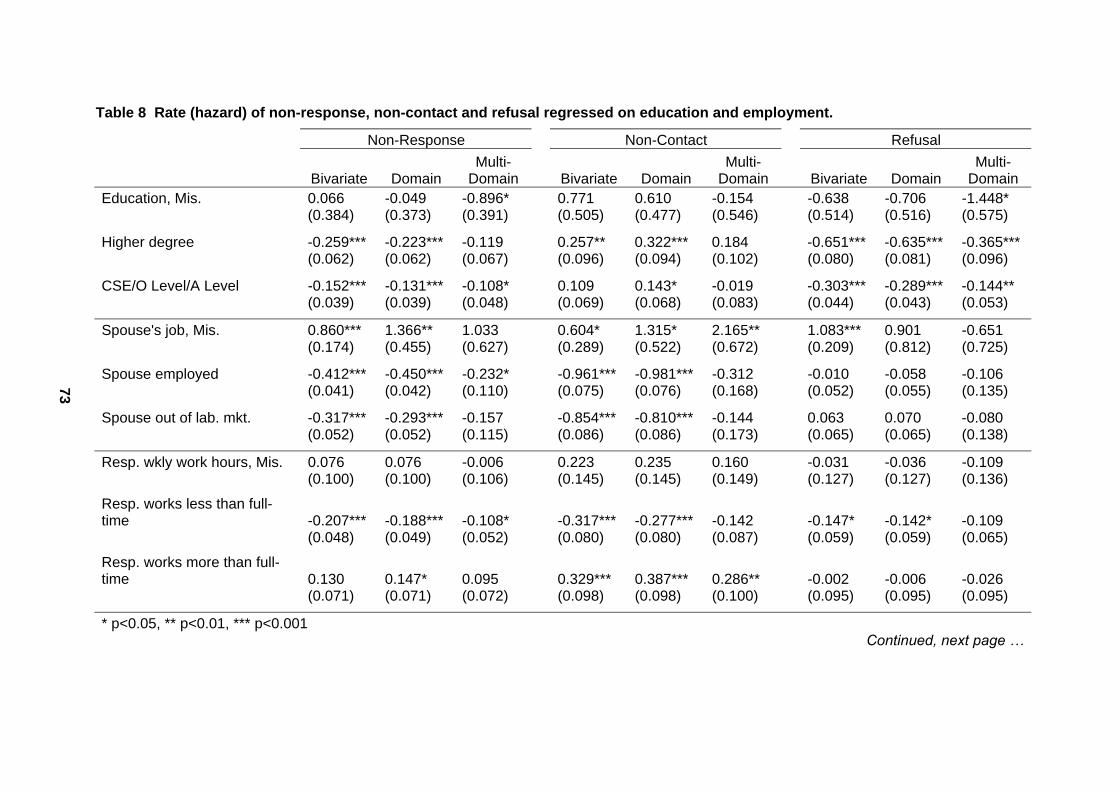
Table 8 Rate (hazard) of non-response, non-contact and refusal regressed on education and employment.

Non-Response Non-Contact Refusal

Bivariate Domain Multi-

Domain Bivariate Domain Multi-

Domain Bivariate Domain Multi-

Domain Education, Mis. 0.066 -0.049 -0.896* 0.771 0.610 -0.154 -0.638 -0.706 -1.448* (0.384) (0.373) (0.391) (0.505) (0.477) (0.546) (0.514) (0.516) (0.575)

Higher degree -0.259*** -0.223*** -0.119 0.257** 0.322*** 0.184 -0.651*** -0.635*** -0.365*** (0.062) (0.062) (0.067) (0.096) (0.094) (0.102) (0.080) (0.081) (0.096)

CSE/O Level/A Level -0.152*** -0.131*** -0.108* 0.109 0.143* -0.019 -0.303*** -0.289*** -0.144** (0.039) (0.039) (0.048) (0.069) (0.068) (0.083) (0.044) (0.043) (0.053)

Spouse's job, Mis. 0.860*** 1.366** 1.033 0.604* 1.315* 2.165** 1.083*** 0.901 -0.651 (0.174) (0.455) (0.627) (0.289) (0.522) (0.672) (0.209) (0.812) (0.725)

Spouse employed -0.412*** -0.450*** -0.232* -0.961*** -0.981*** -0.312 -0.010 -0.058 -0.106 (0.041) (0.042) (0.110) (0.075) (0.076) (0.168) (0.052) (0.055) (0.135)

Spouse out of lab. mkt. -0.317*** -0.293*** -0.157 -0.854*** -0.810*** -0.144 0.063 0.070 -0.080 (0.052) (0.052) (0.115) (0.086) (0.086) (0.173) (0.065) (0.065) (0.138)

Resp. wkly work hours, Mis. 0.076 0.076 -0.006 0.223 0.235 0.160 -0.031 -0.036 -0.109 (0.100) (0.100) (0.106) (0.145) (0.145) (0.149) (0.127) (0.127) (0.136)

Resp. works less than full-time -0.207*** -0.188*** -0.108* -0.317*** -0.277*** -0.142 -0.147* -0.142* -0.109 (0.048) (0.049) (0.052) (0.080) (0.080) (0.087) (0.059) (0.059) (0.065)

Resp. works more than full-time 0.130 0.147* 0.095 0.329*** 0.387*** 0.286** -0.002 -0.006 -0.026 (0.071) (0.071) (0.072) (0.098) (0.098) (0.100) (0.095) (0.095) (0.095)

* p<0.05, ** p<0.01, *** p<0.001

73

Continued, next page …

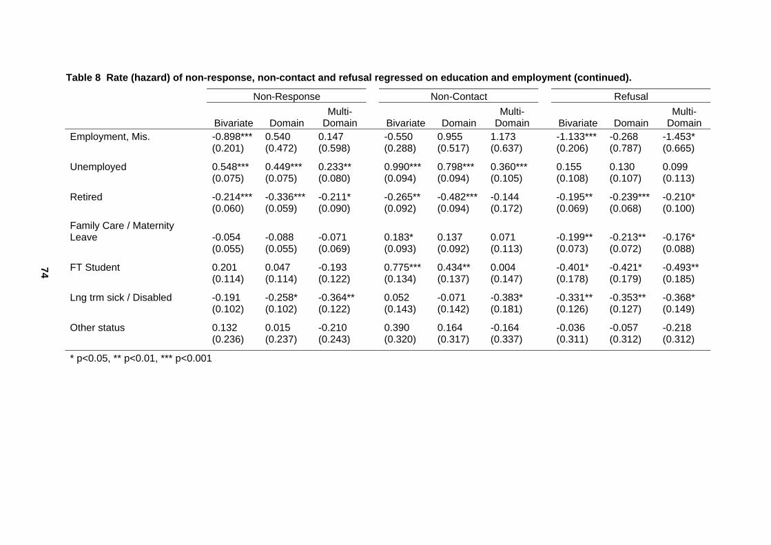
Table 8 Rate (hazard) of non-response, non-contact and refusal regressed on education and employment (continued).

Non-Response Non-Contact Refusal

Bivariate Domain Multi-

Domain Bivariate Domain Multi-

Domain Bivariate Domain Multi-

Domain Employment, Mis. -0.898*** 0.540 0.147 -0.550 0.955 1.173 -1.133*** -0.268 -1.453* (0.201) (0.472) (0.598) (0.288) (0.517) (0.637) (0.206) (0.787) (0.665)

Unemployed 0.548*** 0.449*** 0.233** 0.990*** 0.798*** 0.360*** 0.155 0.130 0.099 (0.075) (0.075) (0.080) (0.094) (0.094) (0.105) (0.108) (0.107) (0.113)

Retired -0.214*** -0.336*** -0.211* -0.265** -0.482*** -0.144 -0.195** -0.239*** -0.210* (0.060) (0.059) (0.090) (0.092) (0.094) (0.172) (0.069) (0.068) (0.100)

Family Care / Maternity Leave -0.054 -0.088 -0.071 0.183* 0.137 0.071 -0.199** -0.213** -0.176* (0.055) (0.055) (0.069) (0.093) (0.092) (0.113) (0.073) (0.072) (0.088)

FT Student 0.201 0.047 -0.193 0.775*** 0.434** 0.004 -0.401* -0.421* -0.493** (0.114) (0.114) (0.122) (0.134) (0.137) (0.147) (0.178) (0.179) (0.185)

Lng trm sick / Disabled -0.191 -0.258* -0.364** 0.052 -0.071 -0.383* -0.331** -0.353** -0.368* (0.102) (0.102) (0.122) (0.143) (0.142) (0.181) (0.126) (0.127) (0.149)

Other status 0.132 0.015 -0.210 0.390 0.164 -0.164 -0.036 -0.057 -0.218 (0.236) (0.237) (0.243) (0.320) (0.317) (0.337) (0.311) (0.312) (0.312)

* p<0.05, ** p<0.01, *** p<0.001

74

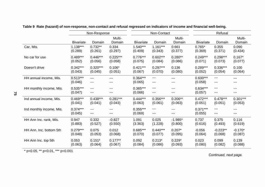
Table 9 Rate (hazard) of non-response, non-contact and refusal regressed on indicators of income and financial well-being.

Non-Response Non-Contact Refusal

Bivariate Domain Multi-

Domain Bivariate Domain Multi-

Domain Bivariate Domain Multi-

Domain Car, Mis. 1.138*** 0.732** 0.334 1.540*** 1.161*** 0.661 0.765* 0.355 0.090 (0.289) (0.261) (0.297) (0.409) (0.343) (0.377) (0.369) (0.371) (0.434)

No car for use 0.489*** 0.446*** 0.225*** 0.776*** 0.602*** 0.280** 0.249*** 0.298*** 0.167* (0.052) (0.056) (0.058) (0.075) (0.084) (0.086) (0.071) (0.073) (0.077)

Doesn't drive 0.342*** 0.320*** 0.106* 0.421*** 0.297*** 0.136 0.289*** 0.336*** 0.100 (0.043) (0.045) (0.051) (0.067) (0.070) (0.080) (0.052) (0.054) (0.064)

HH annual income, Mis. 0.513*** --- --- 0.364*** --- --- 0.600*** --- --- (0.046) --- --- (0.065) --- --- (0.058) --- ---

HH monthly income, Mis. 0.535*** --- --- 0.365*** --- --- 0.634*** --- --- (0.047) --- --- (0.066) --- --- (0.057) --- ---

Ind annual income, Mis. 0.469*** 0.438*** 0.281*** 0.444*** 0.356*** 0.206** 0.472*** 0.478*** 0.301*** (0.041) (0.041) (0.043) (0.063) (0.061) (0.063) (0.051) (0.051) (0.053)

Ind monthly income, Mis. 0.374*** --- --- 0.355*** --- --- 0.371*** --- --- (0.045) --- --- (0.069) --- --- (0.055) --- ---

HH Ann Inc. rank, Mis. 0.947 0.332 -0.827 1.091 0.025 -1.985* 0.737 0.375 0.116 (0.883) (0.527) (0.550) (3.363) (1.228) (0.800) (0.616) (0.493) (0.619)

HH Ann. Inc. bottom 5th 0.279*** 0.075 0.012 0.685*** 0.440*** 0.207* -0.056 -0.223** -0.170* (0.048) (0.053) (0.068) (0.070) (0.077) (0.095) (0.064) (0.068) (0.087)

HH Ann Inc. top 5th 0.053 0.151* 0.177** 0.092 0.213* 0.229* 0.023 0.099 0.139 (0.063) (0.064) (0.067) (0.084) (0.086) (0.093) (0.080) (0.082) (0.088)

* p<0.05, ** p<0.01, *** p<0.001

75

Continued, next page.

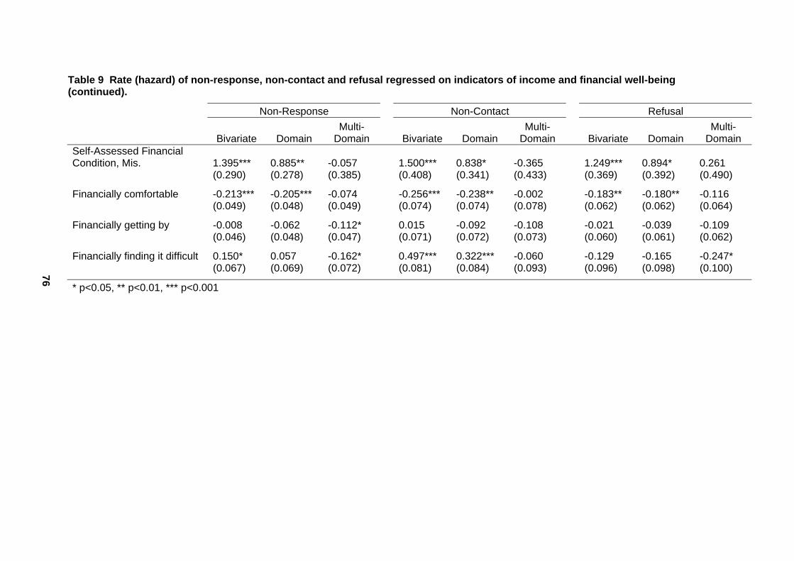
Table 9 Rate (hazard) of non-response, non-contact and refusal regressed on indicators of income and financial well-being (continued).

Non-Response Non-Contact Refusal

Bivariate Domain Multi-

Domain Bivariate Domain Multi-

Domain Bivariate Domain Multi-

Domain Self-Assessed Financial Condition, Mis. 1.395*** 0.885** -0.057 1.500*** 0.838* -0.365 1.249*** 0.894* 0.261 (0.290) (0.278) (0.385) (0.408) (0.341) (0.433) (0.369) (0.392) (0.490)

Financially comfortable -0.213*** -0.205*** -0.074 -0.256*** -0.238** -0.002 -0.183** -0.180** -0.116 (0.049) (0.048) (0.049) (0.074) (0.074) (0.078) (0.062) (0.062) (0.064)

Financially getting by -0.008 -0.062 -0.112* 0.015 -0.092 -0.108 -0.021 -0.039 -0.109 (0.046) (0.048) (0.047) (0.071) (0.072) (0.073) (0.060) (0.061) (0.062)

Financially finding it difficult 0.150* 0.057 -0.162* 0.497*** 0.322*** -0.060 -0.129 -0.165 -0.247* (0.067) (0.069) (0.072) (0.081) (0.084) (0.093) (0.096) (0.098) (0.100)

* p<0.05, ** p<0.01, *** p<0.001

76

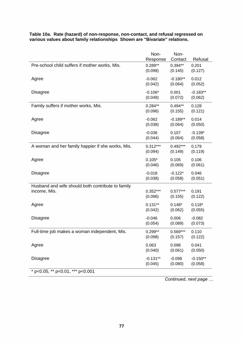
Table 10a. Rate (hazard) of non-response, non-contact, and refusal regressed on various values about family relationships Shown are "Bivariate" relations.

Non-

ResponseNon-

Contact Refusal Pre-school child suffers if mother works, Mis. 0.289** 0.394** 0.201 (0.098) (0.145) (0.127)

Agree -0.062 -0.180** 0.012 (0.042) (0.064) (0.052)

Disagree -0.106* 0.001 -0.183** (0.048) (0.072) (0.062)

Family suffers if mother works, Mis. 0.284** 0.494** 0.128 (0.096) (0.155) (0.121)

Agree -0.062 -0.189** 0.014 (0.038) (0.064) (0.050)

Disagree -0.036 0.107 -0.139* (0.044) (0.064) (0.058)

A woman and her family happier if she works, Mis. 0.312*** 0.492*** 0.179 (0.094) (0.149) (0.119)

Agree 0.105* 0.105 0.106 (0.046) (0.069) (0.061)

Disagree -0.018 -0.122* 0.046 (0.038) (0.058) (0.051)

Husband and wife should both contribute to family income, Mis. 0.352*** 0.577*** 0.191 (0.096) (0.155) (0.122)

Agree 0.131** 0.148* 0.118* (0.042) (0.062) (0.055)

Disagree -0.046 0.006 -0.082 (0.054) (0.089) (0.073)

Full-time job makes a woman independent, Mis. 0.299** 0.569*** 0.110 (0.098) (0.157) (0.122)

Agree 0.063 0.098 0.041 (0.040) (0.061) (0.050)

Disagree -0.131** -0.098 -0.150** (0.045) (0.080) (0.058)

* p<0.05, ** p<0.01, *** p<0.001

Continued, next page …

77

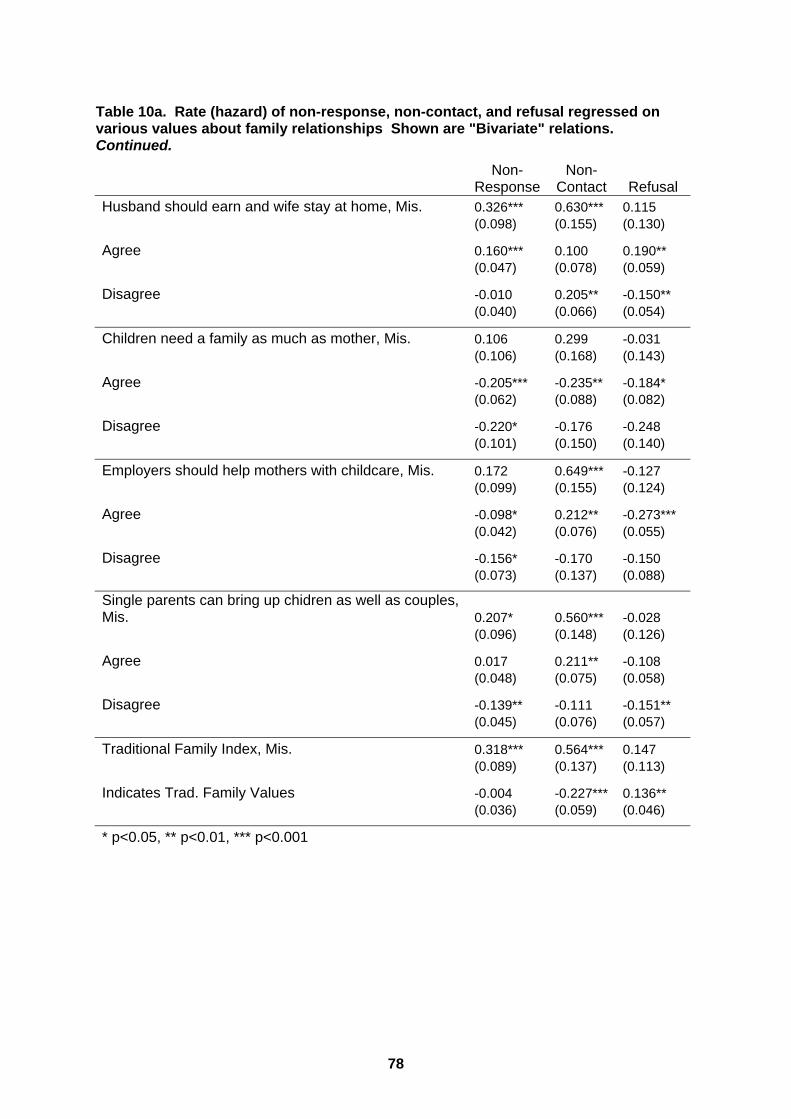
Table 10a. Rate (hazard) of non-response, non-contact, and refusal regressed on various values about family relationships Shown are "Bivariate" relations. Continued.

Non-

ResponseNon-

Contact Refusal Husband should earn and wife stay at home, Mis. 0.326*** 0.630*** 0.115 (0.098) (0.155) (0.130)

Agree 0.160*** 0.100 0.190** (0.047) (0.078) (0.059)

Disagree -0.010 0.205** -0.150** (0.040) (0.066) (0.054)

Children need a family as much as mother, Mis. 0.106 0.299 -0.031 (0.106) (0.168) (0.143)

Agree -0.205*** -0.235** -0.184* (0.062) (0.088) (0.082)

Disagree -0.220* -0.176 -0.248 (0.101) (0.150) (0.140)

Employers should help mothers with childcare, Mis. 0.172 0.649*** -0.127 (0.099) (0.155) (0.124)

Agree -0.098* 0.212** -0.273*** (0.042) (0.076) (0.055)

Disagree -0.156* -0.170 -0.150 (0.073) (0.137) (0.088)

Single parents can bring up chidren as well as couples, Mis. 0.207* 0.560*** -0.028 (0.096) (0.148) (0.126)

Agree 0.017 0.211** -0.108 (0.048) (0.075) (0.058)

Disagree -0.139** -0.111 -0.151** (0.045) (0.076) (0.057)

Traditional Family Index, Mis. 0.318*** 0.564*** 0.147 (0.089) (0.137) (0.113)

Indicates Trad. Family Values -0.004 -0.227*** 0.136** (0.036) (0.059) (0.046)

* p<0.05, ** p<0.01, *** p<0.001

78

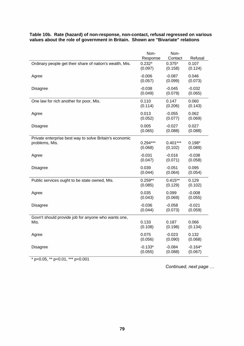
Table 10b. Rate (hazard) of non-response, non-contact, refusal regressed on various values about the role of government in Britain. Shown are "Bivariate" relations

Non-

Response Non-

Contact Refusal Ordinary people get their share of nation's wealth, Mis. 0.232* 0.375* 0.107 (0.097) (0.158) (0.124)

Agree -0.006 -0.087 0.046 (0.057) (0.099) (0.073)

Disagree -0.038 -0.045 -0.032 (0.049) (0.079) (0.065)

One law for rich another for poor, Mis. 0.110 0.147 0.060 (0.114) (0.206) (0.143)

Agree 0.013 -0.055 0.062 (0.052) (0.077) (0.069)

Disagree 0.005 -0.027 0.027 (0.065) (0.088) (0.088)

Private enterprise best way to solve Britain's economic problems, Mis. 0.294*** 0.401*** 0.198* (0.068) (0.102) (0.089)

Agree -0.031 -0.016 -0.038 (0.047) (0.071) (0.058)

Disagree 0.039 -0.051 0.095 (0.044) (0.064) (0.054)

Public services ought to be state owned, Mis. 0.259** 0.415** 0.129 (0.085) (0.129) (0.102)

Agree 0.035 0.099 -0.008 (0.043) (0.069) (0.055)

Disagree -0.036 -0.058 -0.021 (0.044) (0.073) (0.059)

Govn't should provide job for anyone who wants one, Mis. 0.133 0.187 0.066 (0.108) (0.198) (0.134)

Agree 0.075 -0.023 0.132 (0.056) (0.090) (0.068)

Disagree -0.133* -0.084 -0.164* (0.055) (0.088) (0.067)

* p<0.05, ** p<0.01, *** p<0.001

Continued, next page …

79

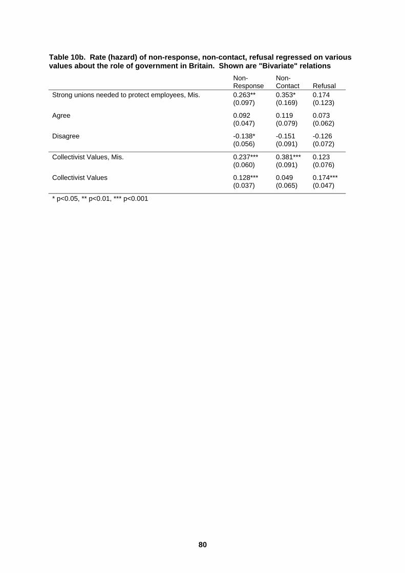
Table 10b. Rate (hazard) of non-response, non-contact, refusal regressed on various values about the role of government in Britain. Shown are "Bivariate" relations

Non- Response

Non- Contact Refusal

Strong unions needed to protect employees, Mis. 0.263** 0.353* 0.174 (0.097) (0.169) (0.123)

Agree 0.092 0.119 0.073 (0.047) (0.079) (0.062)

Disagree -0.138* -0.151 -0.126 (0.056) (0.091) (0.072)

Collectivist Values, Mis. 0.237*** 0.381*** 0.123 (0.060) (0.091) (0.076)

Collectivist Values 0.128*** 0.049 0.174*** (0.037) (0.065) (0.047)

* p<0.05, ** p<0.01, *** p<0.001

80

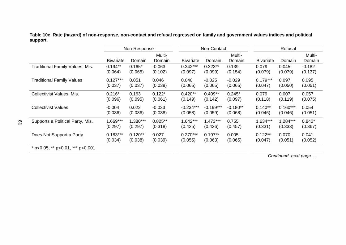
Table 10c Rate (hazard) of non-response, non-contact and refusal regressed on family and government values indices and political support.

Non-Response Non-Contact Refusal

Bivariate Domain Multi-

Domain Bivariate Domain Multi-

Domain Bivariate Domain Multi-

Domain Traditional Family Values, Mis. 0.194** 0.165* -0.063 0.342*** 0.323** 0.139 0.079 0.045 -0.182 (0.064) (0.065) (0.102) (0.097) (0.099) (0.154) (0.079) (0.079) (0.137)

Traditional Family Values 0.127*** 0.051 0.046 0.040 -0.025 -0.029 0.179*** 0.097 0.095 (0.037) (0.037) (0.039) (0.065) (0.065) (0.065) (0.047) (0.050) (0.051)

Collectivist Values, Mis. 0.216* 0.163 0.122* 0.420** 0.409** 0.245* 0.079 0.007 0.057 (0.096) (0.095) (0.061) (0.149) (0.142) (0.097) (0.118) (0.119) (0.075)

Collectivist Values -0.004 0.022 -0.033 -0.234*** -0.199*** -0.180** 0.140** 0.160*** 0.054 (0.036) (0.036) (0.038) (0.058) (0.059) (0.068) (0.046) (0.046) (0.051)

Supports a Political Party, Mis. 1.669*** 1.380*** 0.825** 1.642*** 1.473*** 0.755 1.634*** 1.284*** 0.842* (0.297) (0.297) (0.318) (0.425) (0.426) (0.457) (0.331) (0.333) (0.367)

Does Not Support a Party 0.183*** 0.120** 0.027 0.270*** 0.197** 0.005 0.122** 0.070 0.041 (0.034) (0.038) (0.039) (0.055) (0.063) (0.065) (0.047) (0.051) (0.052)

* p<0.05, ** p<0.01, *** p<0.001

81

Continued, next page …

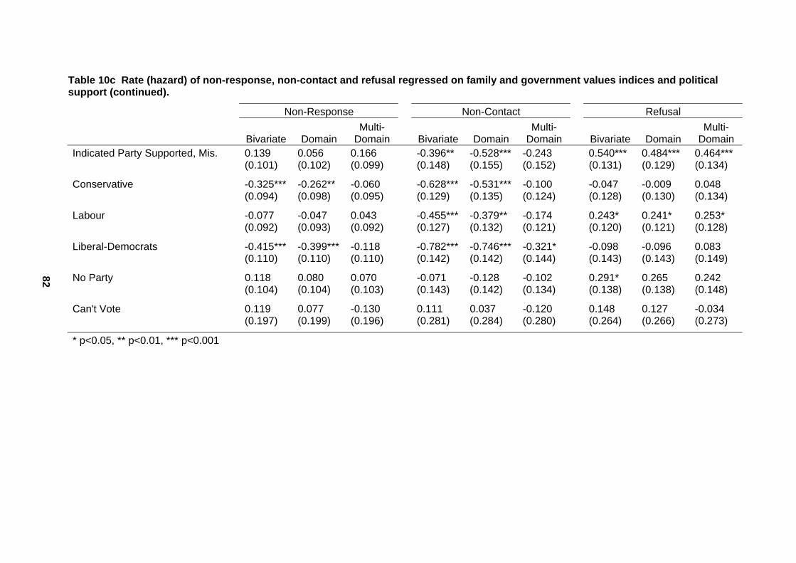
Table 10c Rate (hazard) of non-response, non-contact and refusal regressed on family and government values indices and political support (continued).

Non-Response Non-Contact Refusal

Bivariate Domain Multi-

Domain Bivariate Domain Multi-

Domain Bivariate Domain Multi-

Domain Indicated Party Supported, Mis. 0.139 0.056 0.166 -0.396** -0.528*** -0.243 0.540*** 0.484*** 0.464*** (0.101) (0.102) (0.099) (0.148) (0.155) (0.152) (0.131) (0.129) (0.134)

Conservative -0.325*** -0.262** -0.060 -0.628*** -0.531*** -0.100 -0.047 -0.009 0.048 (0.094) (0.098) (0.095) (0.129) (0.135) (0.124) (0.128) (0.130) (0.134)

Labour -0.077 -0.047 0.043 -0.455*** -0.379** -0.174 0.243* 0.241* 0.253* (0.092) (0.093) (0.092) (0.127) (0.132) (0.121) (0.120) (0.121) (0.128)

Liberal-Democrats -0.415*** -0.399*** -0.118 -0.782*** -0.746*** -0.321* -0.098 -0.096 0.083 (0.110) (0.110) (0.110) (0.142) (0.142) (0.144) (0.143) (0.143) (0.149)

No Party 0.118 0.080 0.070 -0.071 -0.128 -0.102 0.291* 0.265 0.242 (0.104) (0.104) (0.103) (0.143) (0.142) (0.134) (0.138) (0.138) (0.148)

Can't Vote 0.119 0.077 -0.130 0.111 0.037 -0.120 0.148 0.127 -0.034 (0.197) (0.199) (0.196) (0.281) (0.284) (0.280) (0.264) (0.266) (0.273)

* p<0.05, ** p<0.01, *** p<0.001

82

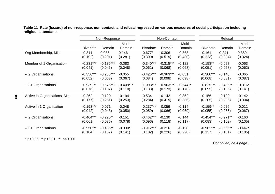
Table 11 Rate (hazard) of non-response, non-contact, and refusal regressed on various measures of social participation including religious attendance.

Non-Response Non-Contact Refusal

Bivariate Domain Multi-

Domain Bivariate Domain Multi-

Domain Bivariate Domain Multi-

Domain Org Membership, Mis. -0.311 0.085 0.146 -0.677* -0.306 -0.368 -0.161 0.241 0.389 (0.192) (0.291) (0.281) (0.300) (0.519) (0.480) (0.223) (0.334) (0.324)

Member of 1 Organisation -0.231*** -0.186*** -0.083 -0.340*** -0.315*** -0.122 -0.153** -0.097 -0.063 (0.041) (0.046) (0.048) (0.061) (0.068) (0.068) (0.051) (0.058) (0.062)

-- 2 Organisations -0.356*** -0.236*** -0.055 -0.426*** -0.363*** -0.051 -0.300*** -0.148 -0.065 (0.052) (0.063) (0.067) (0.084) (0.098) (0.098) (0.068) (0.081) (0.087)

-- 3+ Organisations -0.939*** -0.675*** -0.409*** -1.093*** -0.963*** -0.544** -0.825*** -0.485*** -0.316* (0.076) (0.107) (0.110) (0.133) (0.173) (0.178) (0.095) (0.136) (0.141)

Active in Organisations, Mis. -0.262 -0.120 -0.194 -0.534 -0.142 -0.352 -0.156 -0.129 -0.142 (0.177) (0.261) (0.253) (0.284) (0.419) (0.386) (0.205) (0.295) (0.304)

Active in 1 Organisation -0.193*** -0.071 -0.048 -0.237*** -0.059 -0.114 -0.159** -0.076 -0.011 (0.042) (0.048) (0.050) (0.059) (0.066) (0.069) (0.055) (0.065) (0.067)

-- 2 Organisations -0.464*** -0.220** -0.151 -0.462*** -0.130 -0.144 -0.454*** -0.271** -0.160 (0.061) (0.076) (0.078) (0.096) (0.118) (0.117) (0.083) (0.102) (0.105)

-- 3+ Organisations -0.950*** -0.435** -0.330* -0.912*** -0.216 -0.128 -0.961*** -0.566** -0.447* (0.104) (0.137) (0.141) (0.182) (0.226) (0.228) (0.137) (0.181) (0.185)

* p<0.05, ** p<0.01, *** p<0.001

83

Continued, next page …

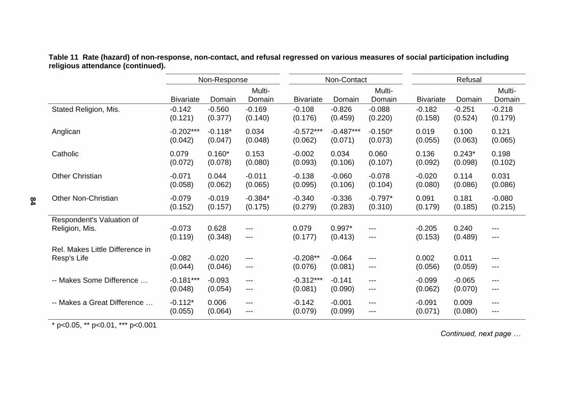
Table 11 Rate (hazard) of non-response, non-contact, and refusal regressed on various measures of social participation including religious attendance (continued).

Non-Response Non-Contact Refusal

Bivariate Domain Multi-

Domain Bivariate Domain Multi-

Domain Bivariate Domain Multi-

Domain Stated Religion, Mis. -0.142 -0.560 -0.169 -0.108 -0.826 -0.088 -0.182 -0.251 -0.218 (0.121) (0.377) (0.140) (0.176) (0.459) (0.220) (0.158) (0.524) (0.179)

Anglican -0.202*** -0.118* 0.034 -0.572*** -0.487*** -0.150* 0.019 0.100 0.121 (0.042) (0.047) (0.048) (0.062) (0.071) (0.073) (0.055) (0.063) (0.065)

Catholic 0.079 0.160* 0.153 -0.002 0.034 0.060 0.136 0.243* 0.198 (0.072) (0.078) (0.080) (0.093) (0.106) (0.107) (0.092) (0.098) (0.102)

Other Christian -0.071 0.044 -0.011 -0.138 -0.060 -0.078 -0.020 0.114 0.031 (0.058) (0.062) (0.065) (0.095) (0.106) (0.104) (0.080) (0.086) (0.086)

Other Non-Christian -0.079 -0.019 -0.384* -0.340 -0.336 -0.797* 0.091 0.181 -0.080 (0.152) (0.157) (0.175) (0.279) (0.283) (0.310) (0.179) (0.185) (0.215)

Respondent's Valuation of Religion, Mis. -0.073 0.628 --- 0.079 0.997* --- -0.205 0.240 --- (0.119) (0.348) --- (0.177) (0.413) --- (0.153) (0.489) ---

Rel. Makes Little Difference in Resp's Life -0.082 -0.020 --- -0.208** -0.064 --- 0.002 0.011 --- (0.044) (0.046) --- (0.076) (0.081) --- (0.056) (0.059) ---

-- Makes Some Difference … -0.181*** -0.093 --- -0.312*** -0.141 --- -0.099 -0.065 --- (0.048) (0.054) --- (0.081) (0.090) --- (0.062) (0.070) ---

-- Makes a Great Difference … -0.112* 0.006 --- -0.142 -0.001 --- -0.091 0.009 --- (0.055) (0.064) --- (0.079) (0.099) --- (0.071) (0.080) ---

* p<0.05, ** p<0.01, *** p<0.001

84

Continued, next page …

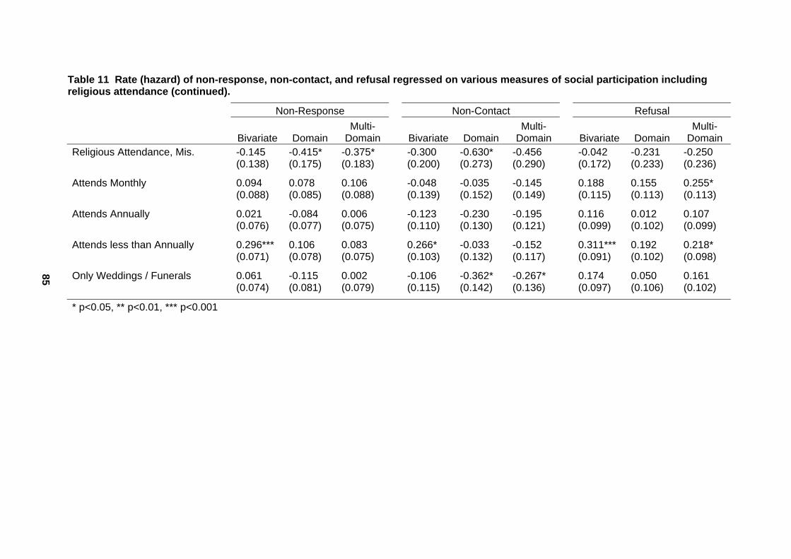
Table 11 Rate (hazard) of non-response, non-contact, and refusal regressed on various measures of social participation including religious attendance (continued).

Non-Response Non-Contact Refusal

Bivariate Domain Multi-

Domain Bivariate Domain Multi-

Domain Bivariate Domain Multi-

Domain Religious Attendance, Mis. -0.145 -0.415* -0.375* -0.300 -0.630* -0.456 -0.042 -0.231 -0.250 (0.138) (0.175) (0.183) (0.200) (0.273) (0.290) (0.172) (0.233) (0.236)

Attends Monthly 0.094 0.078 0.106 -0.048 -0.035 -0.145 0.188 0.155 0.255* (0.088) (0.085) (0.088) (0.139) (0.152) (0.149) (0.115) (0.113) (0.113)

Attends Annually 0.021 -0.084 0.006 -0.123 -0.230 -0.195 0.116 0.012 0.107 (0.076) (0.077) (0.075) (0.110) (0.130) (0.121) (0.099) (0.102) (0.099)

Attends less than Annually 0.296*** 0.106 0.083 0.266* -0.033 -0.152 0.311*** 0.192 0.218* (0.071) (0.078) (0.075) (0.103) (0.132) (0.117) (0.091) (0.102) (0.098)

Only Weddings / Funerals 0.061 -0.115 0.002 -0.106 -0.362* -0.267* 0.174 0.050 0.161 (0.074) (0.081) (0.079) (0.115) (0.142) (0.136) (0.097) (0.106) (0.102)

* p<0.05, ** p<0.01, *** p<0.001

85