The NCEP–NCAR 50-Year Reanalysis: Monthly Means CD-ROM …

247Bulletin of the American Meteorological Society

1. Introduction

The National Centers for Environmental Prediction(NCEP) and National Center for Atmospheric Re-search (NCAR) have cooperated in a project (denoted“reanalysis”) to produce a retroactive record of morethan 50 years of global analyses of atmospheric fieldsin support of the needs of the research and climatemonitoring communities. This effort involved the re-covery of land surface, ship, rawinsonde, pibal, air-craft, satellite, and other data. These data were thenquality controlled and assimilated with a data assimi-lation system kept unchanged over the reanalysis pe-riod. This eliminated perceived climate jumpsassociated with changes in the operational (real time)

data assimilation system, although the reanalysis isstill affected by changes in the observing systems.During the earliest decade (1948–57), there were fewerupper-air data observations and they were made 3 hlater than the current main synoptic times (e.g.,0300 UTC), and primarily in the Northern Hemi-sphere, so that the reanalysis is less reliable than forthe later 40 years. The reanalysis data assimilationsystem continues to be used with current data in realtime (Climate Data Assimilation System or CDAS),so that its products are available from 1948 to thepresent. The products include, in addition to thegridded reanalysis fields, 8-day forecasts every 5 days,and the binary universal format representation (BUFR)archive of the atmospheric observations. The productscan be obtained from NCAR, NCEP, and from theNational Oceanic and Atmospheric Administration/Climate Diagnostics Center (NOAA/CDC). (TheirWeb page addresses can be linked to from the Webpage of the NCEP–NCAR reanalysis at http://wesley.wwb.noaa.gov/Reanalysis.html.)

This issue of the Bulletin includes a CD-ROM witha documentation of the NCEP–NCAR reanalysis(Kistler et al. 1999). In this paper we present a briefsummary and some highlights of the documentation(also available on the Web at http://atmos.umd.edu/~ekalnay/). The CD-ROM, similar to the one issuedwith the March 1996 issue of the Bulletin, contains41 yr (1958–97) of monthly means of many reanaly-sis variables and estimates of precipitation derivedfrom satellite and in situ observations (see the appen-

The NCEP–NCAR 50-Year Reanalysis:Monthly Means CD-ROM

and Documentation

Robert Kistler,* Eugenia Kalnay,+ William Collins,* Suranjana Saha,* Glenn White,*John Woollen,* Muthuvel Chelliah,# Wesley Ebisuzaki,# Masao Kanamitsu,#

Vernon Kousky,# Huug van den Dool,# Roy Jenne,@ and Michael Fiorino&

*Environmental Modeling Center, National Centers for Environ-mental Prediction, Washington, D.C.+Department of Meteorology, University of Maryland, CollegePark, Maryland.#Climate Prediction Center, National Centers for EnvironmentalPrediction, Washington, D.C.#National Center for Atmospheric Research, Boulder, Colorado.&Lawrence Livermore National Laboratory, Livermore, Califor-nia, and European Centre for Medium-Range Weather Forecasts,Reading, United Kingdom.Corresponding author address: Dr. Eugenia Kalnay, Dept. ofMeteorology, University of Maryland, 2213 Computer and SpaceScience Building, College Park, MD 20742-2425.E-mail: [email protected] final form 24 October 2000.©2001 American Meteorological Society

Editor’s note: This article is accompanied by a CD-ROM that contains the complete documentation of theNCEP–NCAR Reanalysis and all of the data analyses and forecasts. It is provided to members through thesponsorship of SAIC and GSC.

248 Vol. 82, No. 2, February 2001

dix for an introduction to the CD-ROM). It also con-tains selected monthly fields for the earlier decade(1948–57). The full CD-ROM contents and the re-analysis for 1999 and later years as well as additionaldetailed documentation and links are also available atthe NCEP–NCAR reanalysis Web site (see also theappendix).

2. Brief description of the reanalysissystem

The reanalysis data assimilation system, describedin more detail in Kalnay et al. (1996), includes theNCEP global spectral model operational in 1995, with28 “sigma” vertical levels and a triangular truncationof 62 waves, equivalent to about 210-km horizontalresolution. The analysis scheme is a three-dimensionalvariational (3DVAR) scheme cast in spectral spacedenoted spectral statistical interpolation (Parrish andDerber 1992). The assimilated observations are upper-air rawinsonde observations of temperature, horizon-tal wind, and specific humidity; operational TelevisionInfrared Observation Satellite (TIROS) OperationalVertical Sounder (TOVS) vertical temperature sound-ings from NOAA polar orbiters over ocean, with mi-crowave retrievals excluded between 20°N and 20°Sdue to rain contamination; TOVS temperature sound-

ings over land only above 100 hPa; cloud-tracked windsfrom geostationary satellites; aircraft observations ofwind and temperature; land surface reports of surfacepressure; and oceanic reports of surface pressure, tem-perature, horizontal wind, and specific humidity.

Gridded variables, the most widely used productof the reanalysis, have been classified into three classes(Kalnay et al. 1996): type A variables, including upper-air temperatures, rotational wind, and geopotentialheight, are generally strongly influenced by the avail-able observations and are therefore the most reliableproduct of the reanalysis. Type B variables, includingmoisture variables, divergent wind, and surface param-eters, are influenced both by the observations and bythe model, and are therefore less reliable. Type C vari-ables, such as surface fluxes, heating rates, and pre-cipitation, are completely determined by the model(subject to the constraint of the assimilation of otherobservations). They should be used with caution andwhenever possible compared with model-independentestimates. It is frequently noted that even when themodel estimates are biased, the interannual variabilitytends to be correlated with independent observations.

Although the reanalysis data assimilation systemis maintained constant, the observing system hasevolved substantially. We can separate the evolutionof the global observing system into three major phases:the “early” period from the 1940s to the International

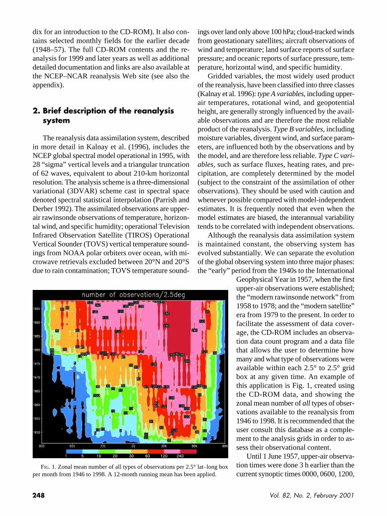
Geophysical Year in 1957, when the firstupper-air observations were established;the “modern rawinsonde network” from1958 to 1978; and the “modern satellite”era from 1979 to the present. In order tofacilitate the assessment of data cover-age, the CD-ROM includes an observa-tion data count program and a data filethat allows the user to determine howmany and what type of observations wereavailable within each 2.5° to 2.5° gridbox at any given time. An example ofthis application is Fig. 1, created usingthe CD-ROM data, and showing thezonal mean number of all types of obser-vations available to the reanalysis from1946 to 1998. It is recommended that theuser consult this database as a comple-ment to the analysis grids in order to as-sess their observational content.

Until 1 June 1957, upper-air observa-tion times were done 3 h earlier than thecurrent synoptic times 0000, 0600, 1200,

FIG. 1. Zonal mean number of all types of observations per 2.5° lat–long boxper month from 1946 to 1998. A 12-month running mean has been applied.


and 1800 UTC. For this reason the reanalysis for thefirst decade (1948–57) is performed at the observingtimes (0300, 0900, 1500, and 2100 UTC). To facili-tate comparisons with later periods, however, the 3-hforecasts and model diagnostic fields are also madeavailable in the reanalysis at the current main synop-tic times. It should be noted that the forecast error co-variance, tuned to the present observing system, waskept constant throughout the reanalysis. This impliesless than optimal information extraction during thepresatellite era.

The documentation in the CD-ROM describes themany different sources of observations put together forthis project, giving an inventory for each data sourceas a function of time. The BUFR observational dataarchive includes “events” or metadata pertaining to theobservation, such as information about quality controland the departure of the observation from both thebackground and the analysis (Woollen and Zhu 1997).We note that in the process of performing the reanaly-sis and constructing the BUFR archive, we discovereda major (and still unresolved) mystery in the opera-tional Global Telecommunication System (GTS). For27 months in the early 1990s geographically differentand complementary rawinsonde data were transmittedin real time to NCEP and to the European Centre forMedium-Range Weather Forecasts (ECMWF) so thateach center had only about half of these data.

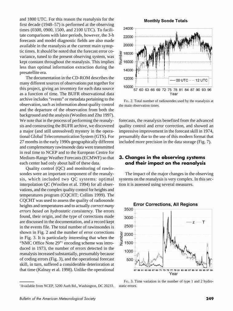
Quality control (QC) and monitoring of rawin-sondes were an important component of the reanaly-sis, which included two QC systems: optimalinterpolation QC (Woollen et al. 1994) for all obser-vations, and the complex quality control for heights andtemperatures program (CQCHT; Collins 1999). TheCQCHT was used to assess the quality of radiosondeheights and temperatures and to actually correct manyerrors based on hydrostatic consistency. The errorsfound, their origin, and the type of corrections madeare discussed in the documentation, and a record keptin the events file. The total number of rawinsondes isshown in Fig. 2 and the number of error correctionsin Fig. 3. It is particularly interesting that when the“NMC Office Note 29”1 encoding scheme was intro-duced in 1973, the number of errors detected in thereanalysis increased substantially, presumably becauseof coding errors (Fig. 3), and the operational forecastskill, in turn, suffered a considerable deterioration atthat time (Kalnay et al. 1998). Unlike the operational

forecasts, the reanalysis benefited from the advancedquality control and error correction, and showed animpressive improvement in the forecast skill in 1974,presumably due to the use of this modern format thatincluded more precision in the data storage (Fig. 7).

3. Changes in the observing systemsand their impact on the reanalysis

The impact of the major changes in the observingsystems on the reanalysis is very complex. In this sec-tion it is assessed using several measures.

FIG. 3. Time variation in the number of type 1 and 2 hydro-static errors.

FIG. 2. Total number of radiosondes used by the reanalysis atthe main observation times.

1Available from NCEP, 5200 Auth Rd., Washington, DC 20233.

250 Vol. 82, No. 2, February 2001

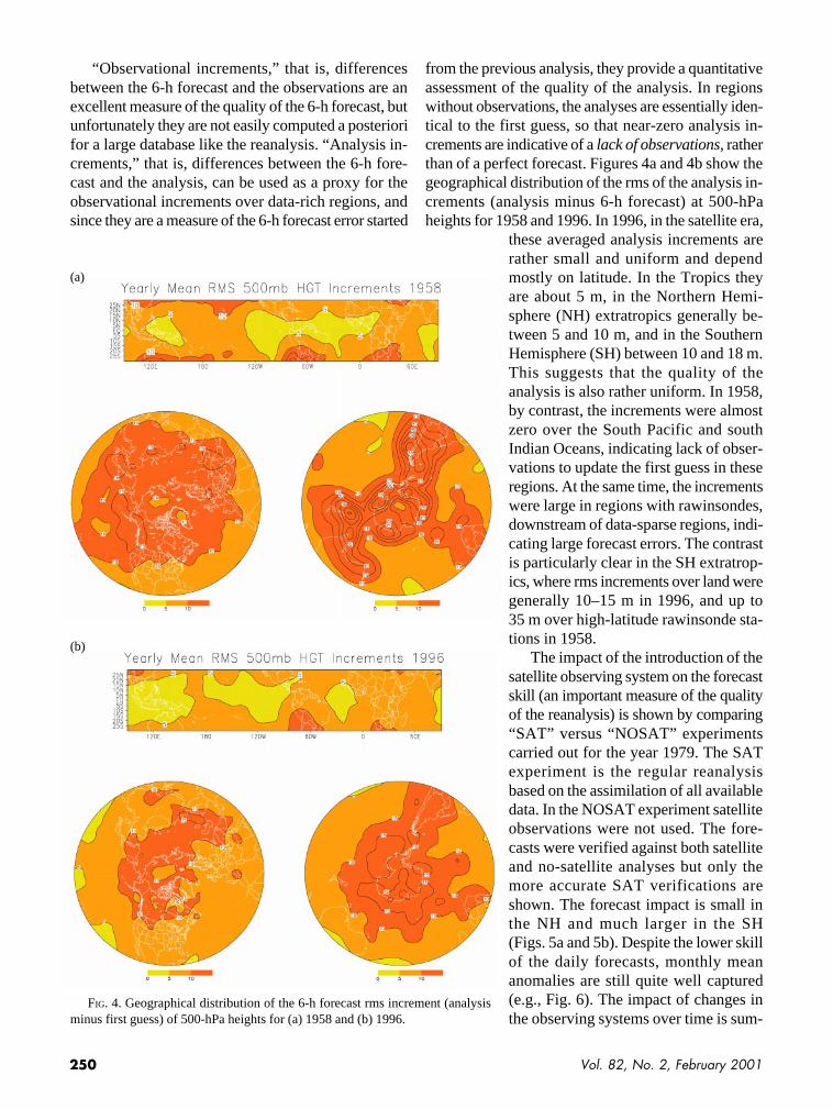
“Observational increments,” that is, differencesbetween the 6-h forecast and the observations are anexcellent measure of the quality of the 6-h forecast, butunfortunately they are not easily computed a posteriorifor a large database like the reanalysis. “Analysis in-crements,” that is, differences between the 6-h fore-cast and the analysis, can be used as a proxy for theobservational increments over data-rich regions, andsince they are a measure of the 6-h forecast error started

from the previous analysis, they provide a quantitativeassessment of the quality of the analysis. In regionswithout observations, the analyses are essentially iden-tical to the first guess, so that near-zero analysis in-crements are indicative of a lack of observations, ratherthan of a perfect forecast. Figures 4a and 4b show thegeographical distribution of the rms of the analysis in-crements (analysis minus 6-h forecast) at 500-hPaheights for 1958 and 1996. In 1996, in the satellite era,

these averaged analysis increments arerather small and uniform and dependmostly on latitude. In the Tropics theyare about 5 m, in the Northern Hemi-sphere (NH) extratropics generally be-tween 5 and 10 m, and in the SouthernHemisphere (SH) between 10 and 18 m.This suggests that the quality of theanalysis is also rather uniform. In 1958,by contrast, the increments were almostzero over the South Pacific and southIndian Oceans, indicating lack of obser-vations to update the first guess in theseregions. At the same time, the incrementswere large in regions with rawinsondes,downstream of data-sparse regions, indi-cating large forecast errors. The contrastis particularly clear in the SH extratrop-ics, where rms increments over land weregenerally 10–15 m in 1996, and up to35 m over high-latitude rawinsonde sta-tions in 1958.

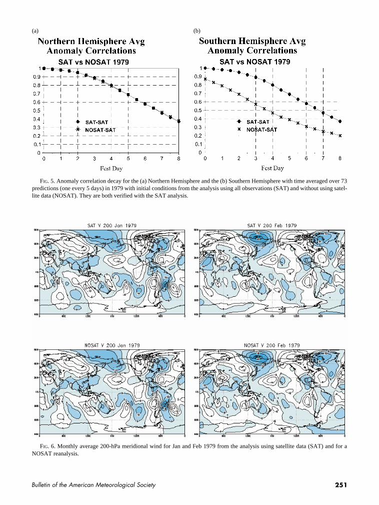
The impact of the introduction of thesatellite observing system on the forecastskill (an important measure of the qualityof the reanalysis) is shown by comparing“SAT” versus “NOSAT” experimentscarried out for the year 1979. The SATexperiment is the regular reanalysisbased on the assimilation of all availabledata. In the NOSAT experiment satelliteobservations were not used. The fore-casts were verified against both satelliteand no-satellite analyses but only themore accurate SAT verifications areshown. The forecast impact is small inthe NH and much larger in the SH(Figs. 5a and 5b). Despite the lower skillof the daily forecasts, monthly meananomalies are still quite well captured(e.g., Fig. 6). The impact of changes inthe observing systems over time is sum-

(b)

FIG. 4. Geographical distribution of the 6-h forecast rms increment (analysisminus first guess) of 500-hPa heights for (a) 1958 and (b) 1996.

(a)


(a) (b)

FIG. 5. Anomaly correlation decay for the (a) Northern Hemisphere and the (b) Southern Hemisphere with time averaged over 73predictions (one every 5 days) in 1979 with initial conditions from the analysis using all observations (SAT) and without using satel-lite data (NOSAT). They are both verified with the SAT analysis.

FIG. 6. Monthly average 200-hPa meridional wind for Jan and Feb 1979 from the analysis using satellite data (SAT) and for aNOSAT reanalysis.

252 Vol. 82, No. 2, February 2001

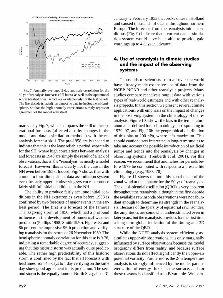
marized by Fig. 7, which compares the skill of the op-erational forecasts (affected also by changes in themodel and data assimilation methods) with the re-analysis forecast skill. The pre-1958 era is shaded toindicate that this is the least reliable period, especiallyfor the SH, where high correlations between analysisand forecasts in 1948 are simply the result of a lack ofobservations, that is, the “reanalysis” is mostly a modelforecast. However, this is clearly not the case in theNH even before 1958. Indeed, Fig. 7 shows that witha modern four-dimensional data assimilation systemeven the early upper-air observing system can producefairly skillful initial conditions in the NH.

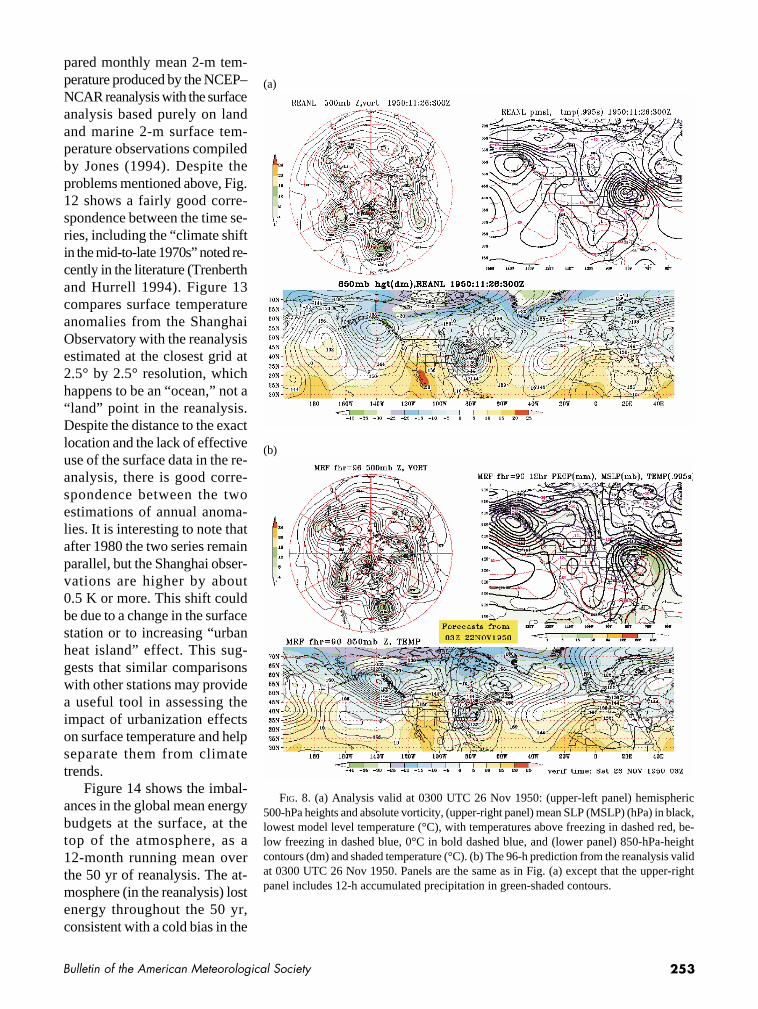
The ability to produce fairly accurate initial con-ditions in the NH extratropics even before 1958 isconfirmed by two forecasts of major events in the ear-liest period. The first is a forecast of the famousThanksgiving storm of 1950, which had a profoundinfluence in the development of numerical weatherprediction (Phillips 1958; Smith 1950). Figures 8a and8b present the impressive 96-h prediction and verify-ing reanalysis for the storm of 26 November 1950. Thehemispheric anomaly correlation for this case is 0.76,indicating a remarkable degree of accuracy, suggest-ing that this historic storm was actually quite predict-able. The rather high predictability of this historicstorm is confirmed by the fact that all forecasts withlead times from 4.5 days to 1 day verifying on the sameday show good agreement in its prediction. The sec-ond storm is the equally famous North Sea gale of 31

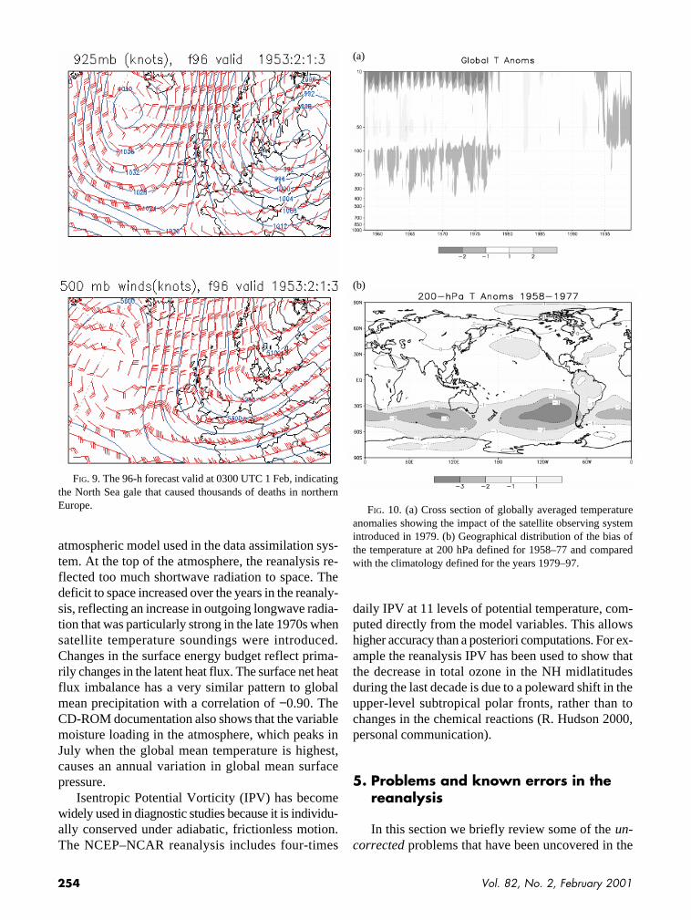
January–2 February 1953 that broke dikes in Hollandand caused thousands of deaths throughout northernEurope. The forecasts from the reanalysis initial con-ditions (Fig. 9) indicate that a current data assimila-tion system would have been able to provide galewarnings up to 4 days in advance.

4. Use of reanalysis in climate studiesand the impact of the observingsystems

Thousands of scientists from all over the worldhave already made extensive use of data from theNCEP–NCAR and other reanalysis projects. Manystudies compare reanalysis output data with varioustypes of real-world estimates and with other reanaly-sis projects. In this section we present several climateapplications, with emphasis on the impact of changesin the observing system on the climatology of the re-analysis. Figure 10a shows the bias in the temperatureanomalies defined for a climatology corresponding to1979–97, and Fig. 10b the geographical distributionof this bias at 200 hPa, where it is maximum. Thisshould caution users interested in long-term studies totake into account the possible introduction of artificialjumps and trends into the reanalysis by changes inobserving systems (Trenberth et al. 2001). For thisreason, we recommend that anomalies for periods be-fore 1979 be computed with respect to a presatelliteclimatology (e.g., 1958–78).

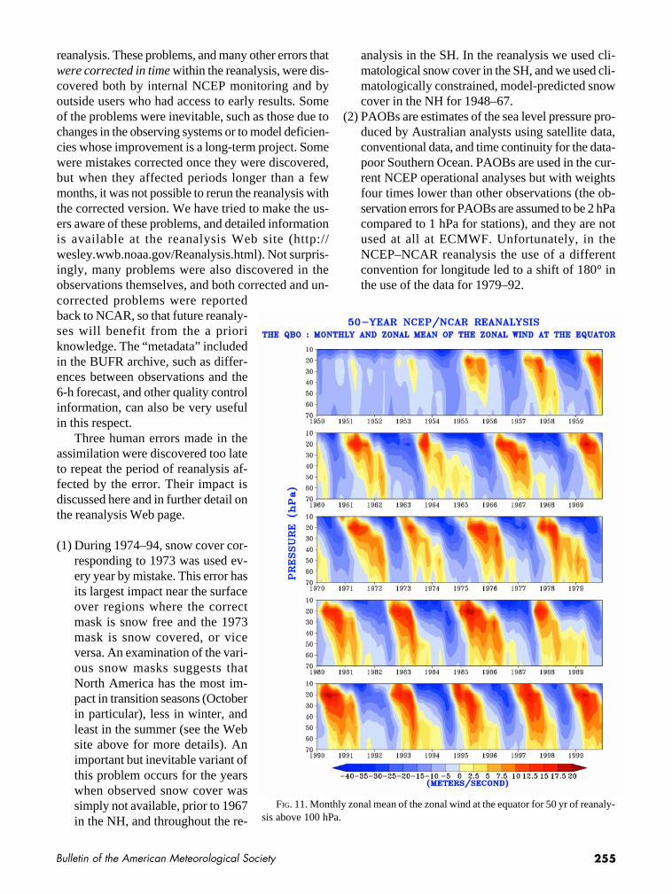
Figure 11 shows the monthly zonal mean of thezonal wind at the equator for the 50 yr of reanalysis.The quasi-biennial oscillation (QBO) is very apparentthroughout the reanalysis, although in the first decadethe available rawinsonde observations were not abun-dant enough to determine its strength in the reanaly-sis. Because of the sparsity of equatorial rawinsondes,the amplitudes are somewhat underestimated even inlater years, but the reanalysis provides for the first timea long-term global indication of the timing and 3Dstructure of the QBO.

While the NCEP analysis system efficiently as-similates upper-air observations, it is only marginallyinfluenced by surface observations because the modelorography differs from reality, and because surfaceobservations do not affect significantly the upper-airpotential vorticity. Furthermore, the 2-m temperatureanalysis is strongly influenced by the model param-eterization of energy fluxes at the surface, and forthese reasons is classified as a B variable. We com-

FIG. 7. Annually averaged 5-day anomaly correlation for the50 yr of reanalysis forecasts (full lines), as well as the operationalscores (dashed lines), which are available only for the last decade.The first decade (shaded) has almost no data in the Southern Hemi-sphere, so that the high anomaly correlations simply representagreement of the model with itself.


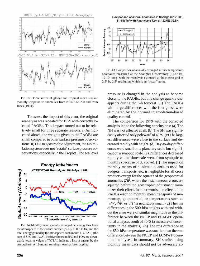
pared monthly mean 2-m tem-perature produced by the NCEP–NCAR reanalysis with the surfaceanalysis based purely on landand marine 2-m surface tem-perature observations compiledby Jones (1994). Despite theproblems mentioned above, Fig.12 shows a fairly good corre-spondence between the time se-ries, including the “climate shiftin the mid-to-late 1970s” noted re-cently in the literature (Trenberthand Hurrell 1994). Figure 13compares surface temperatureanomalies from the ShanghaiObservatory with the reanalysisestimated at the closest grid at2.5° by 2.5° resolution, whichhappens to be an “ocean,” not a“land” point in the reanalysis.Despite the distance to the exactlocation and the lack of effectiveuse of the surface data in the re-analysis, there is good corre-spondence between the twoestimations of annual anoma-lies. It is interesting to note thatafter 1980 the two series remainparallel, but the Shanghai obser-vations are higher by about0.5 K or more. This shift couldbe due to a change in the surfacestation or to increasing “urbanheat island” effect. This sug-gests that similar comparisonswith other stations may providea useful tool in assessing theimpact of urbanization effectson surface temperature and helpseparate them from climatetrends.

Figure 14 shows the imbal-ances in the global mean energybudgets at the surface, at thetop of the atmosphere, as a12-month running mean overthe 50 yr of reanalysis. The at-mosphere (in the reanalysis) lostenergy throughout the 50 yr,consistent with a cold bias in the

FIG. 8. (a) Analysis valid at 0300 UTC 26 Nov 1950: (upper-left panel) hemispheric500-hPa heights and absolute vorticity, (upper-right panel) mean SLP (MSLP) (hPa) in black,lowest model level temperature (°C), with temperatures above freezing in dashed red, be-low freezing in dashed blue, 0°C in bold dashed blue, and (lower panel) 850-hPa-heightcontours (dm) and shaded temperature (°C). (b) The 96-h prediction from the reanalysis validat 0300 UTC 26 Nov 1950. Panels are the same as in Fig. (a) except that the upper-rightpanel includes 12-h accumulated precipitation in green-shaded contours.

(a)

(b)

254 Vol. 82, No. 2, February 2001

atmospheric model used in the data assimilation sys-tem. At the top of the atmosphere, the reanalysis re-flected too much shortwave radiation to space. Thedeficit to space increased over the years in the reanaly-sis, reflecting an increase in outgoing longwave radia-tion that was particularly strong in the late 1970s whensatellite temperature soundings were introduced.Changes in the surface energy budget reflect prima-rily changes in the latent heat flux. The surface net heatflux imbalance has a very similar pattern to globalmean precipitation with a correlation of −0.90. TheCD-ROM documentation also shows that the variablemoisture loading in the atmosphere, which peaks inJuly when the global mean temperature is highest,causes an annual variation in global mean surfacepressure.

Isentropic Potential Vorticity (IPV) has becomewidely used in diagnostic studies because it is individu-ally conserved under adiabatic, frictionless motion.The NCEP–NCAR reanalysis includes four-times

daily IPV at 11 levels of potential temperature, com-puted directly from the model variables. This allowshigher accuracy than a posteriori computations. For ex-ample the reanalysis IPV has been used to show thatthe decrease in total ozone in the NH midlatitudesduring the last decade is due to a poleward shift in theupper-level subtropical polar fronts, rather than tochanges in the chemical reactions (R. Hudson 2000,personal communication).

5. Problems and known errors in thereanalysis

In this section we briefly review some of the un-corrected problems that have been uncovered in the

FIG. 9. The 96-h forecast valid at 0300 UTC 1 Feb, indicatingthe North Sea gale that caused thousands of deaths in northernEurope. FIG. 10. (a) Cross section of globally averaged temperature

anomalies showing the impact of the satellite observing systemintroduced in 1979. (b) Geographical distribution of the bias ofthe temperature at 200 hPa defined for 1958–77 and comparedwith the climatology defined for the years 1979–97.

(a)

(b)


reanalysis. These problems, and many other errors thatwere corrected in time within the reanalysis, were dis-covered both by internal NCEP monitoring and byoutside users who had access to early results. Someof the problems were inevitable, such as those due tochanges in the observing systems or to model deficien-cies whose improvement is a long-term project. Somewere mistakes corrected once they were discovered,but when they affected periods longer than a fewmonths, it was not possible to rerun the reanalysis withthe corrected version. We have tried to make the us-ers aware of these problems, and detailed informationis available at the reanalysis Web site (http://wesley.wwb.noaa.gov/Reanalysis.html). Not surpris-ingly, many problems were also discovered in theobservations themselves, and both corrected and un-corrected problems were reportedback to NCAR, so that future reanaly-ses will benefit from the a prioriknowledge. The “metadata” includedin the BUFR archive, such as differ-ences between observations and the6-h forecast, and other quality controlinformation, can also be very usefulin this respect.

Three human errors made in theassimilation were discovered too lateto repeat the period of reanalysis af-fected by the error. Their impact isdiscussed here and in further detail onthe reanalysis Web page.

(1) During 1974–94, snow cover cor-responding to 1973 was used ev-ery year by mistake. This error hasits largest impact near the surfaceover regions where the correctmask is snow free and the 1973mask is snow covered, or viceversa. An examination of the vari-ous snow masks suggests thatNorth America has the most im-pact in transition seasons (Octoberin particular), less in winter, andleast in the summer (see the Website above for more details). Animportant but inevitable variant ofthis problem occurs for the yearswhen observed snow cover wassimply not available, prior to 1967in the NH, and throughout the re-

analysis in the SH. In the reanalysis we used cli-matological snow cover in the SH, and we used cli-matologically constrained, model-predicted snowcover in the NH for 1948–67.

(2) PAOBs are estimates of the sea level pressure pro-duced by Australian analysts using satellite data,conventional data, and time continuity for the data-poor Southern Ocean. PAOBs are used in the cur-rent NCEP operational analyses but with weightsfour times lower than other observations (the ob-servation errors for PAOBs are assumed to be 2 hPacompared to 1 hPa for stations), and they are notused at all at ECMWF. Unfortunately, in theNCEP–NCAR reanalysis the use of a differentconvention for longitude led to a shift of 180° inthe use of the data for 1979–92.

FIG. 11. Monthly zonal mean of the zonal wind at the equator for 50 yr of reanaly-sis above 100 hPa.

256 Vol. 82, No. 2, February 2001

To assess the impact of this error, the originalreanalysis was repeated for 1979 with correctly lo-cated PAOBs. This impact turned out to be rela-tively small for three separate reasons: i) As indi-cated above, the weights given to the PAOBs aresmall compared to other surface pressure observa-tions. ii) Due to geostrophic adjustment, the assimi-lation system does not “retain” surface pressure ob-servations, especially in the Tropics. The sea level

pressure is changed in the analysis to becomecloser to the PAOBs, but this change quickly dis-appears during the 6-h forecast. iii) The PAOBswith large differences with the first guess wereeliminated by the optimal interpolation–basedquality control.

The comparison for 1979 with the correctedanalysis led to the following conclusions: (a) TheNH was not affected at all. (b) The SH was signifi-cantly affected only poleward of 40°S. (c) The larg-est differences were close to the surface and de-creased rapidly with height. (d) Day-to-day differ-ences were small on a planetary scale but signifi-cant on a synoptic scale. (e) Differences decreasedrapidly as the timescale went from synoptic tomonthly (because of 3, above). (f) The impact onmonthly means of quadratic quantities used forbudgets, transports, etc. is negligible for all crossproducts except for the squares of the geopotentialanomalies

φ′φ′, where the instantaneous errors aresquared before the geostrophic adjustment mini-mizes their effect. In other words, the effect of thePAOBs error on monthly mean transports of mo-mentum, geopotential, or temperatures such asu′v′, v′φ′, or u′T′ is negligibly small. (g) The rmsdifferences in the 500-hPa heights with and with-out the error were of similar magnitude as the dif-ference between the NCEP and ECMWF opera-tional analyses south of 40°S (a measure of uncer-tainty in the analysis). (h) The rms difference inthe 850-hPa temperature was smaller than the rmsdifference between the NCEP and ECMWF opera-tional analyses. In summary, SH studies usingmonthly mean data should not be adversely af-

FIG. 12. Time series of global and tropical mean surfacemonthly temperature anomalies from NCEP–NCAR and fromJones (1994).

FIG. 13. Comparison of annually averaged surface temperatureanomalies measured at the Shanghai Observatory (31.4° lat,121.9° long) with the reanalysis estimated at the closest grid at2.5° by 2.5° resolution, which is an “ocean” point.

FIG. 14. Monthly mean globally averaged net energy flux fromthe atmosphere to the earth’s surface (SFC), at the TOA, and thetotal energy gained by the atmosphere each month (TOTAL) (thesum of SFC and TOA). Positive fluxes in SFC and TOA are down-ward; negative values of TOTAL indicate a loss of energy by theatmosphere. A 12-month running mean has been applied.


fected [except for quadratic perturbations of the sealevel pressure (SLP) or geopotential height].Studies of synoptic-scale features south of 40°S areaffected by the addition of an error that has a mag-nitude comparable to the basic uncertainty of theanalyses. This unfortunate error, which affects thereanalysis from 1980 to 1992, was corrected in theNCEP–Department of Energy (DOE) reanalysis(section 8).

(3)Throughout the reanalysis, the forecast model hada formulation of the horizontal moisture diffusion,which unfortunately caused moisture convergenceleading to unreasonable snowfall over high-latitudevalleys in the winter (“spectral snow”; see Fig. 18near Siberia). This problem has been corrected inthe NCEP operational model as well as in the sec-ond stage of the reanalysis (Reanalysis 2) and isdiscussed in more detail on the reanalysis Web site.The effects are present in the “PRATE” field, buthas been corrected a posteriori in the “XPRATE”model precipitation (which is the one included inthe CD-ROM). However, moisture fluxes cannotbe corrected a posteriori. Another minor modelproblem occurred in the sensible heat flux param-eterization, which allowed surface sensible heatflux to go to zero if the surface wind vanished. Asa result, the surface temperature could occasionallyhave unrealistically high values. This parameter-ization was corrected early during the course of thereanalysis.

6. Comparisons of fluxes estimated bythe NCEP–NCAR, NASA/DAO, andECMWF reanalyses

This section compares fluxes and precipitationfrom the NCEP–NCAR reanalysis discussed in thispaper, the ECMWF 15-yr reanalysis (ERA-15), andthe National Aeronautics and Space Administration(NASA) Data Assimilation Office (DAO) 17-yr re-analysis. Recall that these fields are of type C, that is,produced by the model while it is “nudged” toward theatmosphere during the data assimilation. It is impor-tant to have available several reanalyses to make anestimate of the reliability of their results, especially forquantities and trends that cannot be accurately esti-mated from direct measurements. In this section wecompare reanalyses’ surface and top-of-the-atmo-sphere (TOA) fluxes with independent estimates fromobservations. Section 7 assesses the importance of dif-

ferences in upper-air variables and trends by compar-ing them with interannual variability.

A large number of studies of precipitation and sur-face and top of the atmosphere fluxes in the reanaly-ses were presented at the First and Second WorldClimate Research Programme (WCRP) InternationalConferences on Reanalyses held in 1997 and 1999(WCRP 1998, 2000). A review of several studies ofair–sea fluxes from reanalyses and a comprehensivecomparison of air–sea fluxes from four global reanaly-ses (including the NCEP–DOE reanalysis) with inde-pendent estimates over the period 1981–92 can befound in section 11.4 of the final report of the JointWCRP–Scientific Committee on Oceanic Research(SCOR) Working Group on Air–Sea Fluxes (Taylor2000). Stendahl and Arpe (1997) presented a compre-hensive evaluation of the hydrological cycle in thereanalyses; an updated evaluation can be found in Arpeet al. (2000).

a. Surface energy and momentum fluxesThere is no “ground truth” for most of these fluxes,

since they are not directly measured and have to beestimated indirectly from observations and sometimessignificantly tuned to ensure net energy balance.Satellites, however, directly measure TOA radiativefluxes. In this section we compare monthly mean sur-face fluxes and precipitation as well as TOA radiativefluxes from the three reanalyses to each other and toindependent estimates.

Table 1 shows global mean components of the oceansurface energy balance for the three reanalyses for1981–92. It also shows the da Silva et al. (1994) origi-nal air–sea fluxes averaged over 1981–92 [based onthe Comprehensive Ocean–Atmosphere Data Set(COADS)] and satellite-based estimates of surface netshortwave radiation (NSW) by Darnell et al. (1992)and net longwave radiation by Gupta et al. (1992) av-eraged over July 1983–June 1991. It shows the levelof uncertainty from observational estimates and from thereanalyses for different components of the surface fluxes.

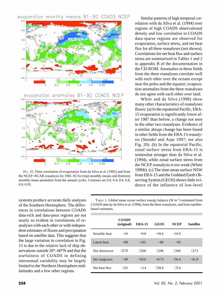
A comparison of ocean surface fluxes from thereanalyses with da Silva et al. (1994) reveals similarpatterns in long-term means and in annual cycles.Temporal correlations of monthly mean evaporationfrom da Silva et al. (1994) with the NCEP–NCARreanalysis for 1981–92 (Fig. 15) are highest where theCOADS observations are most abundant. Operationalforecasts display nearly as much skill in the SouthernHemisphere as in the Northern Hemisphere (Kalnayet al. 1998), indicating that modern data assimilation

258 Vol. 82, No. 2, February 2001

Similar patterns of high temporal cor-relation with da Silva et al. (1994) overregions of high COADS observationaldensity and low correlation in COADSdata-sparse regions are observed forevaporation, surface stress, and net heatflux for all three reanalyses (not shown).Correlations for net heat flux and surfacestress are summarized in Tables 1 and 2in appendix B of the documentation inthe CD-ROM. Anomalies in these fieldsfrom the three reanalyses correlate wellwith each other over the oceans exceptnear the poles and the equator; evapora-tion anomalies from the three reanalysesdo not agree with each other over land.

White and da Silva (1998) showmany other characteristics of reanalysesfluxes: (a) In the equatorial Pacific, ERA-15 evaporation is significantly lower af-ter 1987 than before, a change not seenin the other two reanalyses. Evidence ofa similar abrupt change has been foundin other fields from the ERA-15 reanaly-sis (Stendel and Arpe 1997; see alsoFig. 20). (b) In the equatorial Pacific,zonal surface stress from ERA-15 issomewhat stronger than da Silva et al.(1994), while zonal surface stress fromthe NCEP reanalysis is too weak (White1996b). (c) The time mean surface NSWfrom ERA-15 and the Goddard Earth Ob-serving System (GEOS) shows little evi-dence of the influence of low-level

Sensible heat −10 −9.8 −10.6 −10.9

Latent heat −88 −103 −80 −93

Net shortwave +170 +160 +198 +166 +173

Net longwave −49 −50.6 −67.9 −56.4 −41.9

Net heat flux +23 −3.4 +39.8 +5.6

TABLE 1. Global mean ocean surface energy balance (W m−2) estimated fromCOADS data by da Silva et al. (1994), from the three reanalyses, and from satellite-based estimates.

COADS(original) ERA-15 GEOS NCEP Satellite

FIG. 15. Time correlation of evaporation from da Silva et al. (1992) and fromthe NCEP–NCAR reanalysis for 1981–92 for (top) monthly means and (bottom)monthly mean anomalies from the annual cycles. Contours are 0.0, 0.4, 0.6, 0.8,0.9, 0.95.

systems produce accurate daily analysesof the Southern Hemisphere. The differ-ences in correlations between COADSdata-rich and data-poor regions are notnearly so evident in correlations of re-analyses with each other or with indepen-dent estimates of fluxes and precipitationbased on satellite data. This suggests thatthe large variation in correlation in Fig.15 is due to the relative lack of ship ob-servations outside 20°–60°N and that theusefulness of COADS in defininginterannual variability may be largelylimited to the Northern Hemisphere mid-latitudes and a few other regions.


oceanic stratus clouds, while NCEP’s NSW showsmore evidence of the influence of low-level stratuscloud.

It has been suggested that satellite estimates of sur-face NSW may be more reliable than other global esti-mates of surface NSW, although satellite estimates ofsurface NSW can differ markedly from surface measure-ments (White 1996a). Temporal correlations of reanaly-sis estimates of surface NSW with satellite estimatesof surface NSW by Darnell et al. (1992) are given inTable 3 in appendix B of the documentation in the CD-ROM. ECMWF has more variability in monthly anoma-lies of surface NSW in the Tropics than does the satelliteestimate; NCEP has less than the satellite estimate.

b. Top of the atmosphereAt the TOA, Earth Radiation Balance Experiment

(ERBE) observations of both short- and longwave ra-diation can be compared with the reanalyses. Temporalcorrelations are given in Tables 4 and 5 in appendixB of the documentation in the CD-ROM. The reanaly-ses all have less TOA NSW than ERBE over the tropi-cal oceans, while GEOS has more TOA NSW thanERBE outside the Tropics. The NCEP time meanTOA outgoing longwave radiation (OLR) for 1985–89 is closest to ERBE, while the ERA-15 estimate istoo high and GEOS too low in the Tropics and too highoutside the Tropics. ERA-15 and GEOS display toomuch variability in monthly anomalies of TOA OLRin the Tropics; NCEP has too much variability in mid-latitudes and too little over the tropicaloceans.

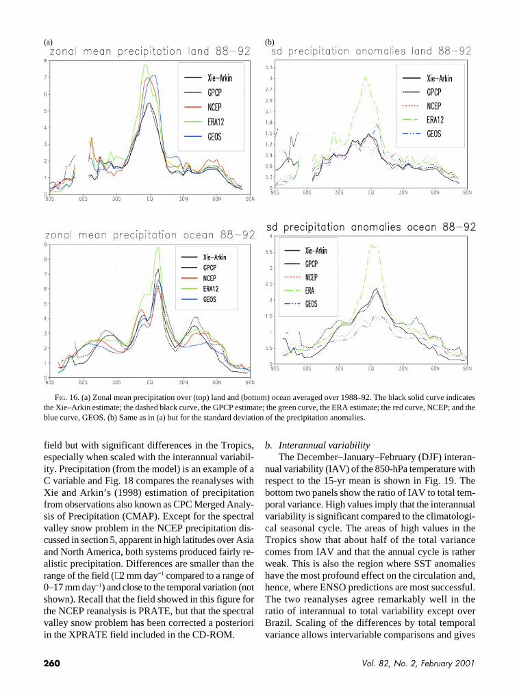
c. PrecipitationFigure 16a compares zonal mean pre-

cipitation over land (top) and ocean (bot-tom) from the three reanalyses with twoindependent estimates by Xie and Arkin(1996, 1998, hereafter XA) and by theGlobal Precipitation Climatology Project(GPCP; WCRP 1990) for 1988–92.Figure 16b compares the standard devia-tion of monthly mean rainfall anomaliesfrom the three reanalyses and from XAover land (top) and ocean (bottom) for1988–92. The results suggest that NCEPand GEOS underestimate variability overthe tropical oceans and the ERA-15 re-analysis substantially overestimates it.All three reanalyses and GPCP havemore variability in oceanic precipitation

at higher latitudes than XA (it should be noted thatinfrared satellite estimates in extratropical latitudes areless reliable). Rms differences from the monthlymeans of XA are shown in Table 2. Of the three re-analyses, ERA has the lowest rms difference over theNorthern Hemisphere continents and the extratropicaloceans, but the largest rms difference over the Trop-ics, especially over land. NCEP has the lowest rms dif-ferences in the Tropics and the largest in the NorthernHemisphere. Table 6 in appendix B in the CD-ROMdocumentation presents temporal correlations of pre-cipitation from the reanalyses and GPCP with the XAestimates.

7. Comparisons of reanalyses estimatesof variables of types A, B, and C

a. Examples of variables of types A, B, and CAs indicated in the introduction, we should expect

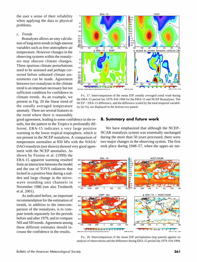
the reanalyses to agree fairly well with each other forfields based on type A variables that are strongly in-fluenced by observations. An example of such a fieldis the zonally averaged u component of the wind,which is primarily nondivergent (Fig. 17) except in theTropics where the model influence is larger and makesit a B variable. The zonally averaged meridional ve-locity, not shown, corresponds to divergent flow andis therefore a B variable. The NCEP–NCAR and ERA-15 reanalyses are qualitatively very similar for the u

a) Land monthly means

Global 1.59 1.41 1.48 0.3920°–80°N 0.81 0.96 1.10 0.2520°S–20°N 3.34 2.51 2.38 0.6720°–80°S 1.28 1.11 1.29 0.35

b) Ocean monthly means

Global 1.81 1.92 1.91 1.2120°–80°N 1.25 1.48 1.51 0.9920°S–20°N 2.84 2.80 2.77 1.8920°–80°S 1.15 1.32 1.31 0.63

TABLE 2. Rms differences in monthly means (mm day−1) over (a) land and (b)ocean in precipitation between the reanalyses and Xie and Arkin (XA) averagedover different regions for 1981–92. Also shown are rms differences in monthlymeans between GPCP and Xie and Arkin for 1988–94.

ERA15-XA GEOS-XA NCEP-XA GPCP-XA

260 Vol. 82, No. 2, February 2001

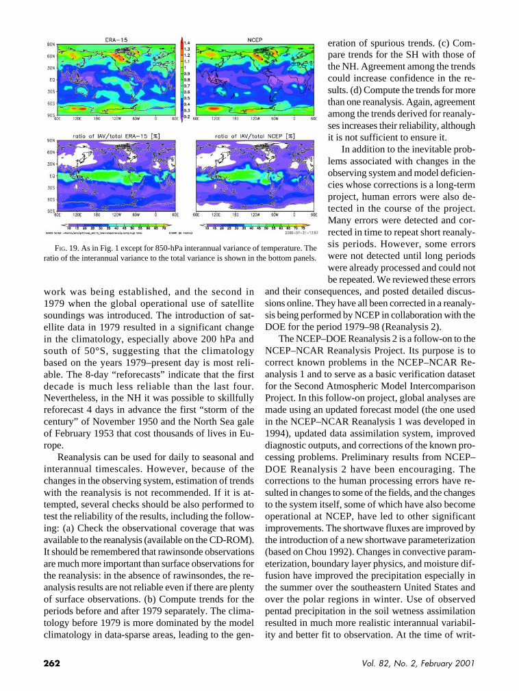
field but with significant differences in the Tropics,especially when scaled with the interannual variabil-ity. Precipitation (from the model) is an example of aC variable and Fig. 18 compares the reanalyses withXie and Arkin’s (1998) estimation of precipitationfrom observations also known as CPC Merged Analy-sis of Precipitation (CMAP). Except for the spectralvalley snow problem in the NCEP precipitation dis-cussed in section 5, apparent in high latitudes over Asiaand North America, both systems produced fairly re-alistic precipitation. Differences are smaller than therange of the field (∼2 mm day−1 compared to a range of0–17 mm day−1) and close to the temporal variation (notshown). Recall that the field showed in this figure forthe NCEP reanalysis is PRATE, but that the spectralvalley snow problem has been corrected a posterioriin the XPRATE field included in the CD-ROM.

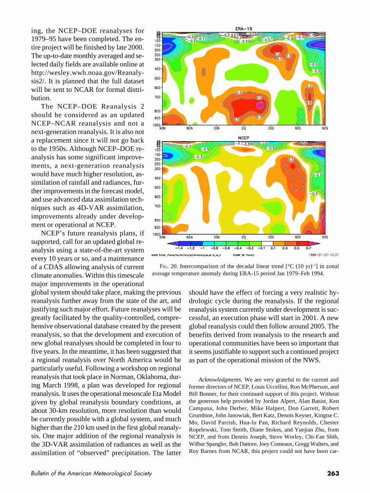
b. Interannual variabilityThe December–January–February (DJF) interan-

nual variability (IAV) of the 850-hPa temperature withrespect to the 15-yr mean is shown in Fig. 19. Thebottom two panels show the ratio of IAV to total tem-poral variance. High values imply that the interannualvariability is significant compared to the climatologi-cal seasonal cycle. The areas of high values in theTropics show that about half of the total variancecomes from IAV and that the annual cycle is ratherweak. This is also the region where SST anomalieshave the most profound effect on the circulation and,hence, where ENSO predictions are most successful.The two reanalyses agree remarkably well in theratio of interannual to total variability except overBrazil. Scaling of the differences by total temporalvariance allows intervariable comparisons and gives

(a) (b)

FIG. 16. (a) Zonal mean precipitation over (top) land and (bottom) ocean averaged over 1988–92. The black solid curve indicatesthe Xie–Arkin estimate; the dashed black curve, the GPCP estimate; the green curve, the ERA estimate; the red curve, NCEP; and theblue curve, GEOS. (b) Same as in (a) but for the standard deviation of the precipitation anomalies.


the user a sense of their reliabilitywhen applying the data to physicalproblems.

c. TrendsReanalyses allows an easy calcula-

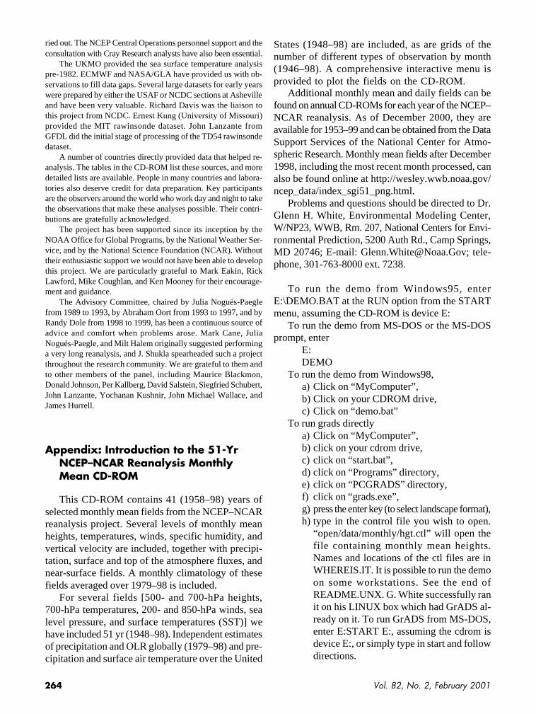
tion of long-term trends in high-interestvariables such as free-atmosphere airtemperature. However changes in theobserving systems within the reanaly-ses may obscure climate changes.These spurious climate perturbationsneed to be assessed and perhaps cor-rected before unbiased climate ass-essments can be made. Agreementbetween two reanalyses in the climatetrend is an important necessary but notsufficient condition for confidence inclimate trends. As an example, wepresent in Fig. 20 the linear trend ofthe zonally averaged temperatureanomaly. There are several features inthe trend where there is reasonablygood agreement, leading to some confidence in the re-sults, but the pattern in the Tropics is profoundly dif-ferent. ERA-15 indicates a very large positivewarming in the lower tropical troposphere, which isnot present in the NCEP reanalysis. A comparison oftemperature anomalies at 850 hPa with the NASA/DAO reanalysis (not shown) showed very good agree-ment with the NCEP anomalies. Asshown by Fiorino et al. (1999) theERA-15 apparent warming resultedfrom an interaction between the modeland the use of TOVS radiances thatlocked in a positive bias during a sud-den and large change in the micro-wave sounding unit channels inNovember 1986 (see also Trenberthet al. 2001).

As indicated before, an importantrecommendation for the estimation oftrends, in addition to the intercom-parison of the reanalyses, is to com-pute trends separately for the periodsbefore and after 1979, and to compareNH and SH trends. Agreement amongthese different estimates should in-crease the confidence in the results.

FIG. 17. Intercomparison of the mean DJF zonally averaged zonal wind duringthe ERA-15 period Jan 1979–Feb 1994 for the ERA-15 and NCEP Reanalyses. TheNCEP − ERA-15 difference, and the difference scaled by the total temporal variabil-ity (in %), are displayed in the bottom two panels.

FIG. 18. Intercomparison of the mean DJF precipitation (top panels) against ananalysis of observations and the difference during ERA-15 period Jan 1979–Feb 1994.

8. Summary and future work

We have emphasized that although the NCEP–NCAR reanalysis system was essentially unchangedduring the more than 50 years processed, there weretwo major changes in the observing system. The firsttook place during 1948–57, when the upper-air net-

262 Vol. 82, No. 2, February 2001

work was being established, and the second in1979 when the global operational use of satellitesoundings was introduced. The introduction of sat-ellite data in 1979 resulted in a significant changein the climatology, especially above 200 hPa andsouth of 50°S, suggesting that the climatologybased on the years 1979–present day is most reli-able. The 8-day “reforecasts” indicate that the firstdecade is much less reliable than the last four.Nevertheless, in the NH it was possible to skillfullyreforecast 4 days in advance the first “storm of thecentury” of November 1950 and the North Sea galeof February 1953 that cost thousands of lives in Eu-rope.

Reanalysis can be used for daily to seasonal andinterannual timescales. However, because of thechanges in the observing system, estimation of trendswith the reanalysis is not recommended. If it is at-tempted, several checks should be also performed totest the reliability of the results, including the follow-ing: (a) Check the observational coverage that wasavailable to the reanalysis (available on the CD-ROM).It should be remembered that rawinsonde observationsare much more important than surface observations forthe reanalysis: in the absence of rawinsondes, the re-analysis results are not reliable even if there are plentyof surface observations. (b) Compute trends for theperiods before and after 1979 separately. The clima-tology before 1979 is more dominated by the modelclimatology in data-sparse areas, leading to the gen-

eration of spurious trends. (c) Com-pare trends for the SH with those ofthe NH. Agreement among the trendscould increase confidence in the re-sults. (d) Compute the trends for morethan one reanalysis. Again, agreementamong the trends derived for reanaly-ses increases their reliability, althoughit is not sufficient to ensure it.

In addition to the inevitable prob-lems associated with changes in theobserving system and model deficien-cies whose corrections is a long-termproject, human errors were also de-tected in the course of the project.Many errors were detected and cor-rected in time to repeat short reanaly-sis periods. However, some errorswere not detected until long periodswere already processed and could notbe repeated. We reviewed these errors

and their consequences, and posted detailed discus-sions online. They have all been corrected in a reanaly-sis being performed by NCEP in collaboration with theDOE for the period 1979–98 (Reanalysis 2).

The NCEP–DOE Reanalysis 2 is a follow-on to theNCEP–NCAR Reanalysis Project. Its purpose is tocorrect known problems in the NCEP–NCAR Re-analysis 1 and to serve as a basic verification datasetfor the Second Atmospheric Model IntercomparisonProject. In this follow-on project, global analyses aremade using an updated forecast model (the one usedin the NCEP–NCAR Reanalysis 1 was developed in1994), updated data assimilation system, improveddiagnostic outputs, and corrections of the known pro-cessing problems. Preliminary results from NCEP–DOE Reanalysis 2 have been encouraging. Thecorrections to the human processing errors have re-sulted in changes to some of the fields, and the changesto the system itself, some of which have also becomeoperational at NCEP, have led to other significantimprovements. The shortwave fluxes are improved bythe introduction of a new shortwave parameterization(based on Chou 1992). Changes in convective param-eterization, boundary layer physics, and moisture dif-fusion have improved the precipitation especially inthe summer over the southeastern United States andover the polar regions in winter. Use of observedpentad precipitation in the soil wetness assimilationresulted in much more realistic interannual variabil-ity and better fit to observation. At the time of writ-

FIG. 19. As in Fig. 1 except for 850-hPa interannual variance of temperature. Theratio of the interannual variance to the total variance is shown in the bottom panels.


ing, the NCEP–DOE reanalyses for1979–95 have been completed. The en-tire project will be finished by late 2000.The up-to-date monthly averaged and se-lected daily fields are available online athttp://wesley.wwb.noaa.gov/Reanaly-sis2/. It is planned that the full datasetwill be sent to NCAR for formal distri-bution.

The NCEP–DOE Reanalysis 2should be considered as an updatedNCEP–NCAR reanalysis and not anext-generation reanalysis. It is also nota replacement since it will not go backto the 1950s. Although NCEP–DOE re-analysis has some significant improve-ments, a next-generation reanalysiswould have much higher resolution, as-similation of rainfall and radiances, fur-ther improvements in the forecast model,and use advanced data assimilation tech-niques such as 4D-VAR assimilation,improvements already under develop-ment or operational at NCEP.

NCEP’s future reanalysis plans, ifsupported, call for an updated global re-analysis using a state-of-the-art systemevery 10 years or so, and a maintenanceof a CDAS allowing analysis of currentclimate anomalies. Within this timescalemajor improvements in the operationalglobal system should take place, making the previousreanalysis further away from the state of the art, andjustifying such major effort. Future reanalyses will begreatly facilitated by the quality-controlled, compre-hensive observational database created by the presentreanalysis, so that the development and execution ofnew global reanalyses should be completed in four tofive years. In the meantime, it has been suggested thata regional reanalysis over North America would beparticularly useful. Following a workshop on regionalreanalysis that took place in Norman, Oklahoma, dur-ing March 1998, a plan was developed for regionalreanalysis. It uses the operational mesoscale Eta Modelgiven by global reanalysis boundary conditions, atabout 30-km resolution, more resolution than wouldbe currently possible with a global system, and muchhigher than the 210 km used in the first global reanaly-sis. One major addition of the regional reanalysis isthe 3D-VAR assimilation of radiances as well as theassimilation of “observed” precipitation. The latter

should have the effect of forcing a very realistic hy-drologic cycle during the reanalysis. If the regionalreanalysis system currently under development is suc-cessful, an execution phase will start in 2001. A newglobal reanalysis could then follow around 2005. Thebenefits derived from reanalysis to the research andoperational communities have been so important thatit seems justifiable to support such a continued projectas part of the operational mission of the NWS.

Acknowledgments. We are very grateful to the current andformer directors of NCEP, Louis Uccellini, Ron McPherson, andBill Bonner, for their continued support of this project. Withoutthe generous help provided by Jordan Alpert, Alan Basist, KenCampana, John Derber, Mike Halpert, Don Garrett, RobertGrumbine, John Janowiak, Bert Katz, Dennis Keyser, Kingtse C.Mo, David Parrish, Hua-lu Pan, Richard Reynolds, ChesterRopelewski, Tom Smith, Diane Stokes, and Yuejian Zhu, fromNCEP, and from Dennis Joseph, Steve Worley, Chi-Fan Shih,Wilbur Spangler, Bob Dattore, Joey Comeaux, Gregg Walters, andRoy Barnes from NCAR, this project could not have been car-

FIG. 20. Intercomparison of the decadal linear trend [°C (10 yr)−1] in zonalaverage temperature anomaly during ERA-15 period Jan 1979–Feb 1994.

264 Vol. 82, No. 2, February 2001

ried out. The NCEP Central Operations personnel support and theconsultation with Cray Research analysts have also been essential.

The UKMO provided the sea surface temperature analysispre-1982. ECMWF and NASA/GLA have provided us with ob-servations to fill data gaps. Several large datasets for early yearswere prepared by either the USAF or NCDC sections at Ashevilleand have been very valuable. Richard Davis was the liaison tothis project from NCDC. Ernest Kung (University of Missouri)provided the MIT rawinsonde dataset. John Lanzante fromGFDL did the initial stage of processing of the TD54 rawinsondedataset.

A number of countries directly provided data that helped re-analysis. The tables in the CD-ROM list these sources, and moredetailed lists are available. People in many countries and labora-tories also deserve credit for data preparation. Key participantsare the observers around the world who work day and night to takethe observations that make these analyses possible. Their contri-butions are gratefully acknowledged.

The project has been supported since its inception by theNOAA Office for Global Programs, by the National Weather Ser-vice, and by the National Science Foundation (NCAR). Withouttheir enthusiastic support we would not have been able to developthis project. We are particularly grateful to Mark Eakin, RickLawford, Mike Coughlan, and Ken Mooney for their encourage-ment and guidance.

The Advisory Committee, chaired by Julia Nogués-Paeglefrom 1989 to 1993, by Abraham Oort from 1993 to 1997, and byRandy Dole from 1998 to 1999, has been a continuous source ofadvice and comfort when problems arose. Mark Cane, JuliaNogués-Paegle, and Milt Halem originally suggested performinga very long reanalysis, and J. Shukla spearheaded such a projectthroughout the research community. We are grateful to them andto other members of the panel, including Maurice Blackmon,Donald Johnson, Per Kallberg, David Salstein, Siegfried Schubert,John Lanzante, Yochanan Kushnir, John Michael Wallace, andJames Hurrell.

Appendix: Introduction to the 51-YrNCEP–NCAR Reanalysis MonthlyMean CD-ROM

This CD-ROM contains 41 (1958–98) years ofselected monthly mean fields from the NCEP–NCARreanalysis project. Several levels of monthly meanheights, temperatures, winds, specific humidity, andvertical velocity are included, together with precipi-tation, surface and top of the atmosphere fluxes, andnear-surface fields. A monthly climatology of thesefields averaged over 1979–98 is included.

For several fields [500- and 700-hPa heights,700-hPa temperatures, 200- and 850-hPa winds, sealevel pressure, and surface temperatures (SST)] wehave included 51 yr (1948–98). Independent estimatesof precipitation and OLR globally (1979–98) and pre-cipitation and surface air temperature over the United

States (1948–98) are included, as are grids of thenumber of different types of observation by month(1946–98). A comprehensive interactive menu isprovided to plot the fields on the CD-ROM.

Additional monthly mean and daily fields can befound on annual CD-ROMs for each year of the NCEP–NCAR reanalysis. As of December 2000, they areavailable for 1953–99 and can be obtained from the DataSupport Services of the National Center for Atmo-spheric Research. Monthly mean fields after December1998, including the most recent month processed, canalso be found online at http://wesley.wwb.noaa.gov/ncep_data/index_sgi51_png.html.

Problems and questions should be directed to Dr.Glenn H. White, Environmental Modeling Center,W/NP23, WWB, Rm. 207, National Centers for Envi-ronmental Prediction, 5200 Auth Rd., Camp Springs,MD 20746; E-mail: [email protected]; tele-phone, 301-763-8000 ext. 7238.

To run the demo from Windows95, enterE:\DEMO.BAT at the RUN option from the STARTmenu, assuming the CD-ROM is device E:

To run the demo from MS-DOS or the MS-DOSprompt, enter

E:DEMO

To run the demo from Windows98,a) Click on “MyComputer”,b) Click on your CDROM drive,c) Click on “demo.bat”

To run grads directlya) Click on “MyComputer”,b) click on your cdrom drive,c) click on “start.bat”,d) click on “Programs” directory,e) click on “PCGRADS” directory,f) click on “grads.exe”,g) press the enter key (to select landscape format),h) type in the control file you wish to open.

“open/data/monthly/hgt.ctl” will open thefile containing monthly mean heights.Names and locations of the ctl files are inWHEREIS.IT. It is possible to run the demoon some workstations. See the end ofREADME.UNX. G. White successfully ranit on his LINUX box which had GrADS al-ready on it. To run GrADS from MS-DOS,enter E:START E:, assuming the cdrom isdevice E:, or simply type in start and followdirections.


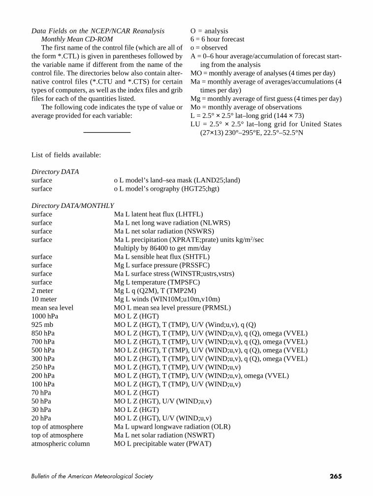
Data Fields on the NCEP/NCAR ReanalysisMonthly Mean CD-ROMThe first name of the control file (which are all of

the form *.CTL) is given in parentheses followed bythe variable name if different from the name of thecontrol file. The directories below also contain alter-native control files (*.CTU and *.CTS) for certaintypes of computers, as well as the index files and gribfiles for each of the quantities listed.

The following code indicates the type of value oraverage provided for each variable:

O = analysis6 = 6 hour forecasto = observedA = 0–6 hour average/accumulation of forecast start-

ing from the analysisMO = monthly average of analyses (4 times per day)Ma = monthly average of averages/accumulations (4

times per day)Mg = monthly average of first guess (4 times per day)Mo = monthly average of observationsL = 2.5° × 2.5° lat–long grid (144 × 73)LU = 2.5° × 2.5° lat–long grid for United States

(27×13) 230°–295°E, 22.5°–52.5°N

List of fields available:

Directory DATAsurface o L model’s land–sea mask (LAND25;land)surface o L model’s orography (HGT25;hgt)

Directory DATA/MONTHLYsurface Ma L latent heat flux (LHTFL)surface Ma L net long wave radiation (NLWRS)surface Ma L net solar radiation (NSWRS)surface Ma L precipitation (XPRATE;prate) units kg/m2/sec

Multiply by 86400 to get mm/daysurface Ma L sensible heat flux (SHTFL)surface Mg L surface pressure (PRSSFC)surface Ma L surface stress (WINSTR;ustrs,vstrs)surface Mg L temperature (TMPSFC)2 meter Mg L q (Q2M), T (TMP2M)10 meter Mg L winds (WIN10M;u10m,v10m)mean sea level MO L mean sea level pressure (PRMSL)1000 hPa MO L Z (HGT)925 mb MO L Z (HGT), T (TMP), U/V (Wind;u,v), q (Q)850 hPa MO L Z (HGT), T (TMP), U/V (WIND;u,v), q (Q), omega (VVEL)700 hPa MO L Z (HGT), T (TMP), U/V (WIND;u,v), q (Q), omega (VVEL)500 hPa MO L Z (HGT), T (TMP), U/V (WIND;u,v), q (Q), omega (VVEL)300 hPa MO L Z (HGT), T (TMP), U/V (WIND;u,v), q (Q), omega (VVEL)250 hPa MO L Z (HGT), T (TMP), U/V (WIND;u,v)200 hPa MO L Z (HGT), T (TMP), U/V (WIND;u,v), omega (VVEL)100 hPa MO L Z (HGT), T (TMP), U/V (WIND;u,v)70 hPa MO L Z (HGT)50 hPa MO L Z (HGT), U/V (WIND;u,v)30 hPa MO L Z (HGT)20 hPa MO L Z (HGT), U/V (WIND;u,v)top of atmosphere Ma L upward longwave radiation (OLR)top of atmosphere Ma L net solar radiation (NSWRT)atmospheric column MO L precipitable water (PWAT)

266 Vol. 82, No. 2, February 2001

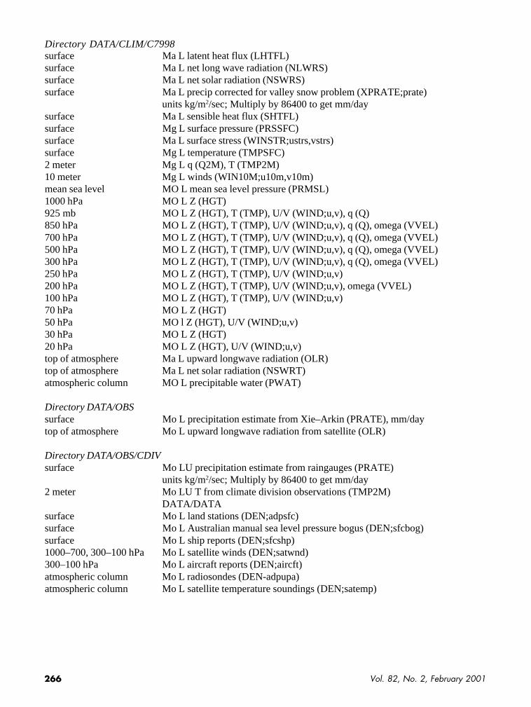
Directory DATA/CLIM/C7998surface Ma L latent heat flux (LHTFL)surface Ma L net long wave radiation (NLWRS)surface Ma L net solar radiation (NSWRS)surface Ma L precip corrected for valley snow problem (XPRATE;prate)

units kg/m2/sec; Multiply by 86400 to get mm/daysurface Ma L sensible heat flux (SHTFL)surface Mg L surface pressure (PRSSFC)surface Ma L surface stress (WINSTR;ustrs,vstrs)surface Mg L temperature (TMPSFC)2 meter Mg L q (Q2M), T (TMP2M)10 meter Mg L winds (WIN10M;u10m,v10m)mean sea level MO L mean sea level pressure (PRMSL)1000 hPa MO L Z (HGT)925 mb MO L Z (HGT), T (TMP), U/V (WIND;u,v), q (Q)850 hPa MO L Z (HGT), T (TMP), U/V (WIND;u,v), q (Q), omega (VVEL)700 hPa MO L Z (HGT), T (TMP), U/V (WIND;u,v), q (Q), omega (VVEL)500 hPa MO L Z (HGT), T (TMP), U/V (WIND;u,v), q (Q), omega (VVEL)300 hPa MO L Z (HGT), T (TMP), U/V (WIND;u,v), q (Q), omega (VVEL)250 hPa MO L Z (HGT), T (TMP), U/V (WIND;u,v)200 hPa MO L Z (HGT), T (TMP), U/V (WIND;u,v), omega (VVEL)100 hPa MO L Z (HGT), T (TMP), U/V (WIND;u,v)70 hPa MO L Z (HGT)50 hPa MO l Z (HGT), U/V (WIND;u,v)30 hPa MO L Z (HGT)20 hPa MO L Z (HGT), U/V (WIND;u,v)top of atmosphere Ma L upward longwave radiation (OLR)top of atmosphere Ma L net solar radiation (NSWRT)atmospheric column MO L precipitable water (PWAT)

Directory DATA/OBSsurface Mo L precipitation estimate from Xie–Arkin (PRATE), mm/daytop of atmosphere Mo L upward longwave radiation from satellite (OLR)

Directory DATA/OBS/CDIVsurface Mo LU precipitation estimate from raingauges (PRATE)

units kg/m2/sec; Multiply by 86400 to get mm/day2 meter Mo LU T from climate division observations (TMP2M)

DATA/DATAsurface Mo L land stations (DEN;adpsfc)surface Mo L Australian manual sea level pressure bogus (DEN;sfcbog)surface Mo L ship reports (DEN;sfcshp)1000–700, 300–100 hPa Mo L satellite winds (DEN;satwnd)300–100 hPa Mo L aircraft reports (DEN;aircft)atmospheric column Mo L radiosondes (DEN-adpupa)atmospheric column Mo L satellite temperature soundings (DEN;satemp)


References

Arpe, K., C. Klepp, and A. Rhodin, 2000: Differences in the hy-drological cycles from different reanalyses—Which one shallwe believe? Proceedings of the 2nd WCRP International Con-ference on Reanalyses, WCRP-109, WMO/TD-985, WorldMeteorological Organization, 193–196.

Chou, M.-D., 1992: A solar radiation model for use in climate stud-ies. J. Atmos. Sci., 49, 762–772.

Collins, W. G., 1999: Monitoring of radiosonde heights and tem-peratures by the complex quality control for the NCEP/NASAReanalysis. NCEP Office note 425, 29 pp. [Available fromNCEP, 5200 Auth Road, Washington, DC 20233.]

da Silva, A., C. C. Young, and S. Levitus, 1994: Atlas of SurfaceMarine Data 1994. Vol. 1: Algorithms and Procedures. NOAAAtlas NESDIS 6, U.S. Department of Commerce, Washington,DC, 83 pp.

Darnell, W. L., W. F. Staylor, S. K. Gupta, N. A. Ritchey, andA. C. Wilber, 1992: Seasonal variation of surface radiationbudget derived from International Satellite Cloud ClimatologyProject C1 Data. J. Geophys. Res., 97, 15 741–15 760.

Fiorino, M., P. Kallberg, and S. Uppala, 1999: The impact of ob-serving system changes on climate scale variability in theNCEP and ECMWF reanalyses. Preprints, 10th Symp. on Glo-bal Change Studies, Dallas, TX, Amer. Meteor. Soc., 119.

Gupta, S., W. Darnell, and A. Wilber, 1992: A parameterizationof long wave surface radiation from satellite data: Recent im-provements. J. Appl. Meteor., 31, 1361–1367.

Jones, P. D., 1994: Recent warming in global temperature series.Geophys. Res. Lett., 21, 1149–1152.

Kalnay, E., and Coauthors, 1996: The NCEP/NCAR 40-YearReanalysis Project. Bull. Amer. Meteor. Soc., 77, 437–471.

——, S. Lord, and R. McPherson, 1998: Maturity of operationalnumerical weather prediction: Medium range. Bull. Amer.Meteor. Soc., 79, 2753–2769.

Kistler, R., and Coauthors, cited 1999: The NCEP/NCAR 50-YearReanalysis. [Available online at http://metosrv2.umd.edu/ekalnay/Reanalysis%20paper/REANCLOS1.html; also avail-able on CD-ROM from Department of Meteorology, Univer-sity of Maryland, College Park, MD 20742.]

Parrish, D. F., and J. C. Derber, 1992: The National Meteorologi-cal Center’s spectral statistical interpolation analysis system.Mon. Wea. Rev., 120, 1747–1763.

Phillips, N. A., 1958: Geostrophic errors in predicting the Appa-lachian storm of November 1950. Geophysica, 6, 389–405.

Smith, C. D., 1950: The destructive storm of November 25–27,1950. Mon. Wea. Rev., 78, 204–209.

Stendahl, M., and K. Arpe, 1997: Evaluation of the hydrologicalcycle in reanalyses and observations. Max-Planck-Institut fürMeteorologie Rep. 228, Hamburg, Germany, 52 pp.

Taylor, P. K., Ed., 2001: Intercomparison and validation of ocean–atmosphere energy flux fields. Joint WCRP/SCOR WorkingGroup on Air–Sea Fluxes Final Rep., WCRP-112, WMO/TD-No. 1036 306 pp. [Available online at http://www.soc.soton.ac.uk/JRD/MET/WGASF.]

Trenberth, K. E., and J. Hurrell, 1994: Decadal atmosphere–oceanvariations in the Pacific. Climate Dyn., 9, 303–319.

——, J. W. Stepaniak, and M. Fiorino, 2001: Quality of reanaly-ses in the Tropics. J. Climate, in press.

——, 1990: Global Precipitation Climatology Project: Implemen-tation and data management plan. World Climate ResearchProgramme, WMO/TD-No. 367, WMO, 47 pp.

WCRP, 1998: Proceedings of the 1st WCRP International Con-ference on Reanalyses. Silver Spring, MD, World Meteoro-logical Organization, WCRP-104, WMO/TD-876, 461 pp.

——, 2000: Proceedings of the 2nd WCRP International Confer-ence on Reanalyses. WCRP-109, WMO/TD-985, World Me-teorological Organization, 452 pp.

White, G., Ed., 1996a: Working Group 2: Existing flux estimates—Their strengths and weaknesses. WCRP Workshop on Air–SeaFluxes for Forcing Ocean Models and Validating GCMs,Reading, United Kingdom, World Meteorological Organiza-tion, WMO/TD-No. 762, xvii–xxxiii.

——, 1996b: Fluxes from the operational analysis/forecast sys-tems and the NCEP/NCAR reanalysis. WCRP Workshop onAir–Sea Flux Fields for Forcing Ocean Models and Validat-ing GCMs, Reading, United Kingdom, WMO/TD-No. 762,131–137.

——, and A. da Silva, 1998: An intercomparison of surface ma-rine fluxes from GEOS-1/DAS, ECMWF/ERA and NCEP/NCAR reanalyses. Preprints, Ninth Conf. on Interaction of theSea and Atmosphere, Phoenix, AZ, Amer. Meteor. Soc., 20–23.

Woollen, J. S., and Y. Zhu, 1997: The NCEP/NCAR reanalysisobservation archive, 1957–1997. Proc. First WCRP Int. Conf.on Reanalyses, Silver Spring, MD WCRP-104, WMO/TD-876,402–405.

——, E. Kalnay, L. Gandin, W. Collins, S. Saha, R. Kistler,M. Kanamitsu, and M. Chelliah, 1994: Quality control in thereanalysis system. Preprints, 10th Conf. on Numerical WeatherPrediction, Portland, OR, Amer. Meteor. Soc., 13–14.

Xie, P., and P. A. Arkin, 1996: Analyses of global monthly pre-cipitation using gauge observations, satellite estimates, andnumerical model predictions. J. Climate, 9, 840–858.

——, and ——, 1998: Global precipitation: A 17-year monthlyanalysis based on gauge observations, satellite estimates, andnumerical model outputs. Bull. Amer. Meteor. Soc., 78, 2539–2558.

268 Vol. 82, No. 2, February 2001

ACCESS TO THE ENTIRE AMSJOURNAL ARCHIVES IS HERE!Currently, AMS Journals Online coverthe period from 1997 to the present. Inresponse to requests by the commu-nity to extend access to include yearsprior to 1997, and in an effort to allowscientists and students to efficientlygain access to a broader and more his-torical perspective on their current re-search, the Society is pleased to offerthe AMS Legacy Journals Online. Fora fixed, one-time price, subscribersmay purchase perpetual online accessto every article published prior to1997 in any or all of our journals(back to 1974 for Monthly WeatherReview). Search capability at the title,author, abstract, and full-text levelsmakes the Legacy an incredibly pow-erful and exciting research tool. The table below shows the number of years of back issuesthat will be available for each issue.

For ordering

information for AMS

Legacy Journals

Online, see the AMS

Web site for details.

Please direct all

other inquiries to

the American

Meteorological

Society by e-mail at

[email protected]

or by telephone at

617-227-2425.

Documents

The NCEP–NCAR 50-Year Reanalysis: Monthly Means CD-ROM …