The Neural Particle Filter

Anna Kutschireiter*1 Simone Carlo Surace1 Henning Sprekeler2 Jean-Pascal Pfister1

1 Institute of Neuroinformatics, University of Zurich and ETH Zurich, Zurich,Switzerland2 Institute of Software Engineering and Theoretical Computer Science, TechnischeUniversitat Berlin, Berlin, Germany

* annak@ini.uzh.ch

Abstract

The robust estimation of dynamically changing features, such as the position of prey, isone of the hallmarks of perception. On an abstract, algorithmic level, nonlinearBayesian filtering, i.e. the estimation of temporally changing signals based on thehistory of observations, provides a mathematical framework for dynamic perception inreal time. Since the general, nonlinear filtering problem is analytically intractable,particle filters are considered among the most powerful approaches to approximatingthe solution numerically. Yet, these algorithms prevalently rely on importance weights,and thus it remains an unresolved question how the brain could implement such aninference strategy with a neuronal population. Here, we propose the Neural ParticleFilter (NPF), a weight-less particle filter that can be interpreted as the neuronaldynamics of a recurrently connected neural network that receives feed-forward inputfrom sensory neurons and represents the posterior probability distribution in terms ofsamples. Specifically, this algorithm bridges the gap between the computational task ofonline state estimation and an implementation that allows networks of neurons in thebrain to perform nonlinear Bayesian filtering. The model captures not only theproperties of temporal and multisensory integration according to Bayesian statistics, butalso allows online learning with a maximum likelihood approach. With an example frommultisensory integration, we demonstrate that the numerical performance of the modelis adequate to account for both filtering and identification problems. Due to theweightless approach, our algorithm alleviates the ’curse of dimensionality’ and thusoutperforms conventional, weighted particle filters in higher dimensions for a limitednumber of particles.

Author Summary

Every day, our brain is facing the challenge of making sense of the rich and dynamicalstream of sensory inputs. Those inputs are often ambiguous, noisy and sometimes evenconflicting. That we are nevertheless able to make sense of our surrounding naturallypoints to the important question how estimates of real-world variables that led toperceptive input, e.g. the position or the velocity of an object, are formed. Further, it isunknown how the computational task of real-time state estimation can be implementedin a realistic neuronal architecture. Here, we propose an algorithm, the Neural ParticleFilter, that performs state estimation, in a way that captures essential properties ofperception: it takes into account prior knowledge of the environment, weights differentsensory modalities according to their reliability and is able to dynamically adapt to

1/23

arX

iv:1

508.

0681

8v2

[q-

bio.

NC

] 3

0 N

ov 2

016

changes. Implemented as a neuronal dynamics, the Neural Particle Filter predictsactivation properties of the neurons involved in perception.

Introduction

During the last decade, an increasing number of studies have stated that the brainperforms probabilistic inference during perceptual tasks [1, 2]. As an act of(approximate) Bayesian inference, perception relies on noisy and incomplete data thatneeds to be integrated across multiple sensory modalities and weighted according tosensory reliability. In addition, perception makes use of the strong statistical regularitiesof objects in our environment by forming prior beliefs about the world. Since ourenvironment is fundamentally dynamic, the ability to adapt to changes in real time isessential for perception. The Bayesian brain hypothesis is supported by ampleexperimental evidence, ranging from psychophysical findings [3–5] to neuronalrecordings [6–8] that are in line with Bayesian computation. However, most of thestudies concerned with the theory of perception consider fairly simple tasks, where theobservations are created either from static hidden variables [9] or from hidden variableswith a discrete state-space [10], or the underlying dynamics are considered linear [11,12].

In a dynamical setting, where temporally changing signals have to be estimatedonline from the history of observations, Bayesian inference is commonly referred to as‘filtering’. In general, nonlinear Bayesian filtering is a challenging task even without theimperative of a plausible implementation on a neuronal architecture. If the priordistribution is a Gaussian and the noisy observations depend linearly on the hiddenstates, the inference problem is solved by the Kalman filter [13,14], which has receivedsubstantial attention in the signal processing community and turns out to be ofincreasing importance in neuroscientific phenomenological modeling, e.g. in asensorimotor integration task [3] or in estimating motor disturbances from an adaptivegain [15]. Solutions for the more general nonlinear, i.e. non-Gaussian, filteringproblem [16,17] are analytically intractable and thus have to be approximated.

Sampling-based approaches have proven to be a powerful tool to solve the nonlinearfiltering problem numerically. In principle, they enable any posterior distribution to berepresented with an accuracy that depends on the number of samples. On the one hand,so called particle methods (see for instance [18, 19]) are well suited for dynamical priors,but suffer in high dimensions due to the degeneracy of the importance weights and it isstill unclear how to implement such an inference scheme in a neuronal network. On theother hand, Langevin sampling [20, 21] and related techniques, such as the ‘fast sampler’in [22], provide a promising ground for a biologically plausible implementation of neuralor synaptic sampling [23,24], but are restricted to static generative models.

Following a sampling-based approach, we propose a framework for how the braincould perform filtering from noisy sensory stimuli, considering Marr’s three levels [25]:the computational level, the algorithmic and representational level and theimplementation level. On the first level, the computational task of dynamical stateestimation is set in the context of continuous-time continuous-state nonlinear filteringtheory. Motivated by this rigorous mathematical theory, we propose a weight-lessparticle filter, the Neural Particle Filter (NPF), that approximates the posterior at eachtime step by sampling from it. This algorithm can further be tuned by maximumlikelihood learning and thus allows for rigorous corrections in the algorithmic ansatz, aswell as learning the model parameters. The NPF exhibits properties that are consideredcrucial for perception. On the implementation level, we interpret the NPF as abiologically plausible neuronal dynamics and identify the particle states with activitiesof task-specific neurons.

2/23

Results

The results we are presenting are subdivided in two parts: first, we will introduce theNeural Particle Filter as a conceptual result. This first part will cover the first two ofMarr’s three levels, namely i.) the computational level with a generative model layoutand a task description, and ii.) the algorithmic level, which outlines our choice ofrepresentation and the approximate solution to the nonlinear filtering problem that isbased on this representation. In the second part, we demonstrate key properties of theNPF, and we we illustrate how they might serve as a model for a neuronal dynamicsinvolved in perception.

Model

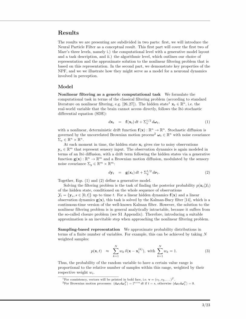
Nonlinear filtering as a generic computational task We formulate thecomputational task in terms of the classical filtering problem (according to standardliterature on nonlinear filtering, e.g. [26, 27]). The hidden state1 xt ∈ Rn, i.e. thereal-world variable that the brain cannot access directly, follows the Ito stochasticdifferential equation (SDE):

dxt = f(xt) dt+ Σ1/2x dωt, (1)

with a nonlinear, deterministic drift function f(x) : Rn → Rn. Stochastic diffusion isgoverned by the uncorrelated Brownian motion process2 ωt ∈ Rn with noise covarianceΣx ∈ Rn × Rn.

At each moment in time, the hidden state xt gives rise to noisy observationsys ∈ Rm that represent sensory input. The observation dynamics is again modeled interms of an Ito diffusion, with a drift term following the hidden states via a generativefunction g(x) : Rn → Rm and a Brownian motion diffusion, modulated by the sensorynoise covariance Σy ∈ Rm × Rm:

dyt = g(xt) dt+ Σ1/2y dνt. (2)

Together, Eqs. (1) and (2) define a generative model.Solving the filtering problem is the task of finding the posterior probability p(xt|Yt)

of the hidden state, conditioned on the whole sequence of observationsYt = {ys, s ∈ [0, t]} up to time t. For a linear hidden dynamics f(x) and a linearobservation dynamics g(x), this task is solved by the Kalman-Bucy filter [14], which is acontinuous-time version of the well-known Kalman filter. However, the solution to thenonlinear filtering problem is in general analytically intractable, because it suffers fromthe so-called closure problem (see S1 Appendix). Therefore, introducing a suitableapproximation is an inevitable step when approaching the nonlinear filtering problem.

Sampling-based representation We approximate probability distributions interms of a finite number of variables. For example, this can be achieved by taking Nweighted samples:

p(x, t) ≈N∑k=1

wk δ(x− x(k)t ), with

N∑k=1

wk = 1. (3)

Thus, the probability of the random variable to have a certain value range isproportional to the relative number of samples within this range, weighted by theirrespective weight wi.

1For consistency, vectors will be printed in bold face, i.e. v = (v1, v2, . . . )T .2For Brownian motion processes: 〈dωtdωT

s 〉 = In×n dt if t = s, otherwise 〈dωtdωTs 〉 = 0.

3/23

Filtering algorithms representing the posterior in this sampling-based manner arecommonly referred to as particle filters. In standard particle filters (such as outlined

in [28]), update rules for the trajectories x(k)t , as well as the weights wk are given.

Despite asymptotic convergence to the true posterior for an infinite number of particles,this approach has two disadvantages: First, one finds numerically that after a finitenumber of time-steps most particle weights decay to zero, which depletes the number ofeffective samples. Weight decay, or degeneration, is an undesirable trait of weightedparticle methods in general. As stated in the convergence theorem [29, Theorem 23.5],the upper bound of the divergence between true posterior and the posterior estimatedby the weighted particle system is a function of time, and hence might be growing dueto the weight decay. Second, the problem is exacerbated if the number of dimensions ofthe hidden state xt is large. In this case, the number of particles needed for goodnumerical performance grows exponentially with the number of dimension, a variant ofthe ‘curse of dimensionality’ [30].

In the theoretical neuroscience literature, sampling-based approaches for filteringwith a representation of the posterior as in Eq. (3) have not received much attention sofar (one of the few examples can be found in [31]), although they have someexperimental support [7, 32] and are considered relevant according to the neuralsampling hypothesis [33]. Therefore, we would like to explore this approach further. Toovercome the difficulties encountered with weighted approaches, we consider a particlefilter with equally weighted samples, i.e. wk = 1/N ∀k.

Filtering with the Neural Particle Filter As an inference algorithm, we proposean SDE that governs the dynamics of particles zt. Let us consider N i.i.d. stochastic

processes z(k)t , k = 1, . . . , N , conditioned on the observations Yt, following the Ito

diffusion

dz(k)t = f(z

(k)t ) dt+Wt

(dyt − g(z

(k)t ) dt

)+ Σ1/2

x dwt, (4)

where wt ∈ Rn is an uncorrelated vector Brownian motion process and Wt is atime-dependent gain matrix or decoding weight matrix.

Equation (4), which we will further refer to as the Neural Particle Filter (NPF)3, isan ansatz that serves as a sampling-based approximation to the nonlinear filtering

problem: we consider each of the N stochastic processes z(k)t as an independent sample,

or particle, of the true posterior p(xt|Yt) at every time t. Thus, expectations from the

posterior are computed according to E[φ(xt)|Yt] ≈ 〈φ(xt)〉 = 1/N∑k φ(z

(k)t ).

This ansatz is motivated by the formal solution to the filtering problem, moreprecisely by the dynamics of the first posterior moment4 and shares some importantproperties with classical filtering methods: First, it is governed by both the dynamics ofthe hidden process xt and by a correction proportional to the so-called innovation termdnt = dyt − g(zt) dt. The innovation term compares the sensory input dyt with thecurrent prediction g(zt) dt according to the single particle position, and thus can beseen as a predictive error signal [9]. Second, the gain matrix Wt determines theemphasis that is laid on new information via observations dyt. This is conceptuallysimilar to a Kalman gain [13,14] for a linear model, and adjusts according to thereliability of a single or multiple observations.

3In the consecutive section, we will identify the particles with neuronal activities, which is why wecall it Neural Particle Filter. Though the name is similar, our NPF is not to be confused with the‘neural filtering’ approach in [34], which is an unsupervised learning algorithm in an artificial neuralnetwork.

4See S1 Appendix for an outline of the formal solution and the dynamics of the first posteriormoment.

4/23

The gain introduces a weighting between the prior probability distribution p(xt)induced by Eq. (1), and the likelihood function p(yt|xt) induced by Eq. (2) and thusserves as a measure for the peakedness of the likelihood. If the decoding weight is large,the dynamics in Eq. (4) will entirely be determined by the innovation term, and theinter-particle variability governed by the diffusion term will be negligible. Therefore, theresulting probability distribution is given by p(xt|Yt) ≈ p(zt|Yt) ∼ δ(zt − g−1(dyt

dt )). Inthis limit, the deterministic observation limit, a single sample from Eq. (4) suffices torepresent the posterior. On the other hand, if the decoding weight is zero, newinformation is disregarded, and each sample evolves just like an i.i.d. process fromEq. (1).4 In this case, the resulting probability distribution simply equals the stationaryprior distribution p(xt).

For the gain Wt, we use the ansatz Wt = cov(xt,g(xt)T )Σ−1

y , an empirical choicemotivated by the mean dynamics of the formal solution5. This gain adjusts according tothe observation noise Σy as well as to the spatial ambiguity as measured by theempirical, i.e. instantaneously estimated from the particle positions, covariance betweenthe state xt and the observation function g(xt) (Eq. 13 in Methods). Although thischoice is rather heuristic, it achieves a numerical performance comparable to that of astandard particle filter (PF), as demonstrated below, and is moreover straightforward toimplement by empirically estimate the covariance from the particle positions.

Parameter learning In a more general setting, model parameters of Eqs. (1) and (2)may not or only partially be known, and thus need to be learned online from the streamof observations Yt. In this case, the NPF algorithm can be extended to include aparameter update that performs an online gradient ascent on the log likelihood

Lonlinet (θ) = 〈g(xt)〉TΣ−1

y dyt −1

2〈g(xt)〉TΣ−1

y 〈g(xt)〉 dt, (5)

which in turn is computed directly from the approximated filtering distribution itself6.It can be shown that maximizing this log likelihood is equivalent to minimizing theprediction error in continuous time (see S1 Appendix).

Further, not only the model parameters in Eqs. (1) and (2), but also the decodingparameters, i.e. components of the decoding weight or gain matrix Wt, can be learnedwith a maximum likelihood approach, instead of setting it according to the empiricalestimate from the particle positions. This alternative corrects for the heuristic ansatz ofthe NPF equation (4) by determining the decoding weights rigorously. In fact, it can beshown that parameter learning with a maximum likelihood approach is able to make upeven for a very poor filtering ansatz by setting parameters accordingly [35].

The Neural Particle Filter as a neuronal dynamics forperception

In this section, we set the computational task in the context of perception and base theimplementation of the algorithm on a neuronal architecture. With a simple example, wenow illustrate that our algorithm captures the following key properties of perception [2]:1) it relies on noisy and incomplete sensory data, 2) it uses prior knowledge of thedynamic structure of the environment 3) it efficiently combines information from severalsensory modalities, and 4) it can dynamically adapt to changes in the environment.

5See footnote 4.6via 〈g(xt)〉 ≈ N−1

∑k g(z

(k)t ), Eq. (20) in Methods

5/23

Multisensory perception as filtering

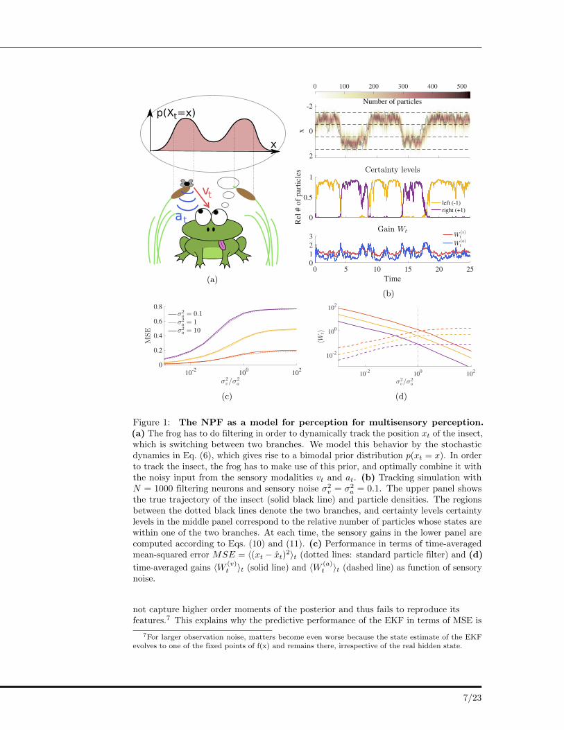
Consider a frog who sits below two branches and observes an insect flying between thetwo branches (Fig. 1a). The frog wants to track the position of the insect xt, which isgoverned by

dxt = 3xt(1− x2t

)dt+ dωt, (6)

where the Brownian motion process ωt accounts for noise due to the erratic behavior ofthe insect. This dynamics gives rise to a bimodal stationary distribution for the positionof the insect (cf. Fig. 1a).

The frog cannot directly observe the state xt of the insect, but instead has to rely ontwo sensory channels, a visual (vt) and an auditory (at) channel. Observation dynamicsin these channels are given by

dvt = xt dt+ σvdβt, (7)

dat = tanh(2xt) dt+ σadγt, (8)

where βt, γt are independent Brownian motions that model noise in the sensorychannels, making vt and at conditionally independent. The nonlinearity in the auditorychannel (Eq. 8) is motivated by the fact that sound localization depends on interauraldifference, which resembles a sigmoid in this example. In order to localize the fly, thefrog has to perform the task of nonlinear filtering and to computext = E[xt|vs, as, 0 ≤ s ≤ t], i.e. the position of the insect, from the visual and auditorysensory streams. Note that due to the nonlinear dynamics of the hidden and observationprocesses, this example is analytically intractable and thus requires an approximation.

We propose that this task is solved by a set of N filtering neurons zit, i = 1, ..., N .Their neuronal dynamics are given by the NPF (4) and for this particular example read:

dz(i)t = 3z

(i)t

(1− (z

(i)t )2

)dt+ dω

(i)t

+W(v)t

(dvt − z(i)t dt

)+W

(a)t

(dat − tanh(2z

(i)t ) dt

), (9)

which is governed by the dynamics of the prior as well as corrections evoked by novelty

of the observations in the sensory channels, that are modulated by gains W(v)t and

W(a)t . Thus, our model readily captures the first two key properties of perception.

The empirical distribution of neuronal activities z(i)t approximately samples the

posterior distribution, thereby acting as a weight-less particle filter that successfullytracks the position of the insect (Fig. 1b). The state estimate xt (posterior mean) canbe read out from this population by averaging the activities of the filtering neurons,

i.e. xt ≈ 〈zt〉 = N−1∑i z

(i)t .

The potential of having a description of the full posterior stretches far beyondsimple state estimation, where one is only interested in the first moment. Particularlythe sampling-based approximation of this posterior allows a convenient estimation ofother relevant quantities. For example, the frog might want to know on which branchthe insect is sitting in order to catch it more easily. The frog could directly deduce acertainty level for the left and right branch, respectively (Fig. 1b), by counting thenumber of neurons within a certain activity range.

In a similar manner, higher-order moments of the posterior distribution can beapproximated with the samples that correspond to neuronal activities. Even thoughthese approximated moments are not exact (Fig. 2c), the overall posterior shape iscaptured to a considerable extent. For some nonlinearities, our proposed model istherefore superior to models relying on an approximation of just the first two momentsof the distribution. For instance, the Extended Kalman Filter (EKF) does by definition

6/23

p(X =x)

x

t

v

a

t

t

(a)

-2

0

2

x

0 100 200 300 400 500

Number of particles

0

0.5

1

Rel

# o

f par

ticl

es

Certainty levels

left (-1)right (+1)

0 5 10 15 20 25

Time

0

1

2

3

Gain WtW

(v)t

W(a)t

(b)

10-2

100

102

σ2v/σ

2a

0

0.2

0.4

0.6

0.8

MSE

σ2a = 0.1

σ2a = 1

σ2a = 10

(c)

10-2

100

102

σ2v/σ

2a

10-2

100

102

⟨Wt⟩

(d)

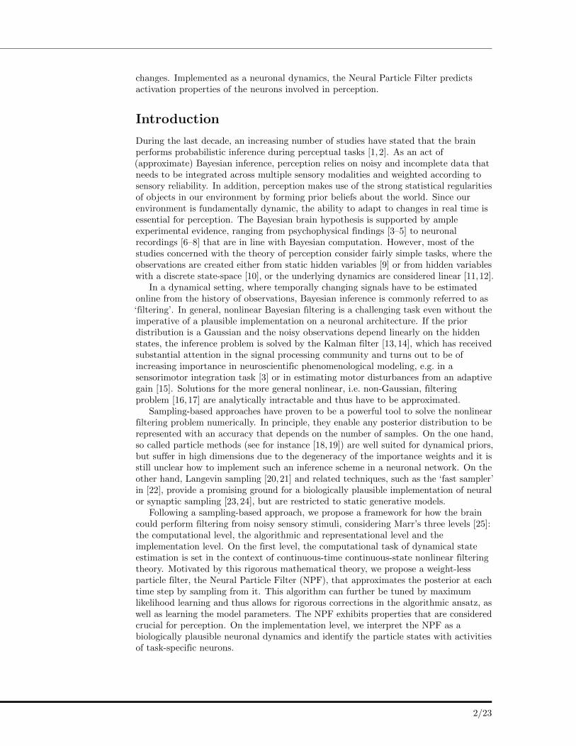
Figure 1: The NPF as a model for perception for multisensory perception.(a) The frog has to do filtering in order to dynamically track the position xt of the insect,which is switching between two branches. We model this behavior by the stochasticdynamics in Eq. (6), which gives rise to a bimodal prior distribution p(xt = x). In orderto track the insect, the frog has to make use of this prior, and optimally combine it withthe noisy input from the sensory modalities vt and at. (b) Tracking simulation withN = 1000 filtering neurons and sensory noise �2

v = �2a = 0.1. The upper panel shows

the true trajectory of the insect (solid black line) and particle densities. The regionsbetween the dotted black lines denote the two branches, and certainty levels certaintylevels in the middle panel correspond to the relative number of particles whose states arewithin one of the two branches. At each time, the sensory gains in the lower panel arecomputed according to Eqs. (10) and (11). (c) Performance in terms of time-averagedmean-squared error MSE = h(xt � xt)

2it (dotted lines: standard particle filter) and (d)

time-averaged gains hW (v)t it (solid line) and hW (a)

t it (dashed line) as function of sensorynoise.

not capture higher order moments of the posterior and thus fails to reproduce its 210

features.7 This explains why the predictive performance of the EKF in terms of MSE is 211

fairly poor compared to that of the NPF (Fig. 2a,b). 212

7For larger observation noise, matters become even worse because the state estimate of the EKFevolves to one of the fixed points of f(x) and remains there, irrespective of the real hidden state.

PLOS 7/21

Figure 1: The NPF as a model for perception for multisensory perception.(a) The frog has to do filtering in order to dynamically track the position xt of the insect,which is switching between two branches. We model this behavior by the stochasticdynamics in Eq. (6), which gives rise to a bimodal prior distribution p(xt = x). In orderto track the insect, the frog has to make use of this prior, and optimally combine it withthe noisy input from the sensory modalities vt and at. (b) Tracking simulation withN = 1000 filtering neurons and sensory noise σ2

v = σ2a = 0.1. The upper panel shows

the true trajectory of the insect (solid black line) and particle densities. The regionsbetween the dotted black lines denote the two branches, and certainty levels certaintylevels in the middle panel correspond to the relative number of particles whose states arewithin one of the two branches. At each time, the sensory gains in the lower panel arecomputed according to Eqs. (10) and (11). (c) Performance in terms of time-averagedmean-squared error MSE = 〈(xt − xt)2〉t (dotted lines: standard particle filter) and (d)

time-averaged gains 〈W (v)t 〉t (solid line) and 〈W (a)

t 〉t (dashed line) as function of sensorynoise.

not capture higher order moments of the posterior and thus fails to reproduce itsfeatures.7 This explains why the predictive performance of the EKF in terms of MSE is

7For larger observation noise, matters become even worse because the state estimate of the EKFevolves to one of the fixed points of f(x) and remains there, irrespective of the real hidden state.

7/23

10-3

10-2

10-1

100

101

102

σ2v

10-2

10-1

100

MSE/V

ar(x

t)

MSE, visual

NPFNPF with MLPFEKF

(a)

10-3

10-2

10-1

100

101

102

σ2a

10-2

10-1

100

MSE/V

ar(x

t)

MSE, auditory

(b)

10-3

10-2

10-1

100

101

102

σ2v , σ

2a

-0.3

-0.2

-0.1

0Bias(Σ)/⟨Σ

PF⟩ t

Bias of estimated variance Σ

(c)

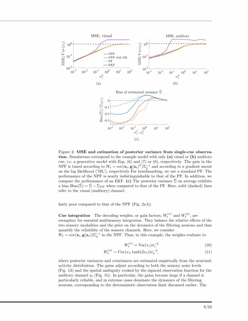
Fig 2: MSE and estimation of posterior variance from single-cue observation.Simulations correspond to the example model with only (a) visual or (b) auditory cue,i.e. a generative model with Eqs. (6) and (7) or (8), respectively. The gain in the NPFis tuned according to Wt = cov(xt,g(xt)

T )⌃�1y and according to a gradient ascent on

the log likelihood (‘ML’). For benchmarking, we use a standard PF. The performanceof the NPF is nearly indistinguishable to that of the PF. In addition, we comparethe performance of an EKF. (c) The posterior variance ⌃ on average exhibits a biasBias(⌃) = ⌃� ⌃PF when compared to that of the PF. Here, solid (dashed) lines referto the visual (auditory) channel.

PLOS 9/23

Figure 2: MSE and estimation of posterior variance from single-cue observa-tion. Simulations correspond to the example model with only (a) visual or (b) auditorycue, i.e. a generative model with Eqs. (6) and (7) or (8), respectively. The gain in theNPF is tuned according to Wt = cov(xt,g(xt)

T )Σ−1y and according to a gradient ascent

on the log likelihood (‘ML’), respectively For benchmarking, we use a standard PF. Theperformance of the NPF is nearly indistinguishable to that of the PF. In addition, wecompare the performance of an EKF. (c) The posterior variance Σ on average exhibitsa bias Bias(Σ) = Σ− ΣPF when compared to that of the PF. Here, solid (dashed) linesrefer to the visual (auditory) channel.

fairly poor compared to that of the NPF (Fig. 2a,b).

Cue integration The decoding weights, or gain factors, W(v)t and W

(a)t , are

exemplary for essential multisensory integration. They balance the relative effects of thetwo sensory modalities and the prior on the dynamics of the filtering neurons and thusquantify the reliability of the sensory channels. Here, we considerWt = cov(xt,g(xt))Σ

−1y in the NPF. Thus, in this example, the weights evaluate to

W(v)t = Var(xt)σ

−2v (10)

W(a)t = Cov(xt, tanh(2xt))σ

−2a , (11)

where posterior variances and covariances are estimated empirically from the neuronalactivity distribution. The gains adjust according to both the sensory noise levels(Fig. 1d) and the spatial ambiguity evoked by the sigmoid observation function for theauditory channel at (Fig. 1b). In particular, the gains become large if a channel isparticularly reliable, and in extreme cases dominate the dynamics of the filteringneurons, corresponding to the deterministic observation limit discussed earlier. The

8/23

appropriate weighting of sensory information allows the neurons to solve the filteringtask near-optimally and comparable to a standard PF, which is reflected by oursimulation results in Fig. 1c and 2a,b.

Adapting to changes In our example, the frog could successfully track the positionof the insect, but it could only do so because it had access to the generative modelparameters, i.e. it knew the prior dynamics of the insect and it it was aware of how thesensory percepts were generated from the true state of the insect. Also, knowledge of

these model parameters were crucial for determining the sensory weights W(v)t and

W(a)t and thus significantly influenced the dynamics of the filtering neurons. However,

the external world, i.e. the model parameters, does change over time, and successfulperception should adapt accordingly, i.e. the model parameters should be adjusted byonline learning from the stream of observations Yt.

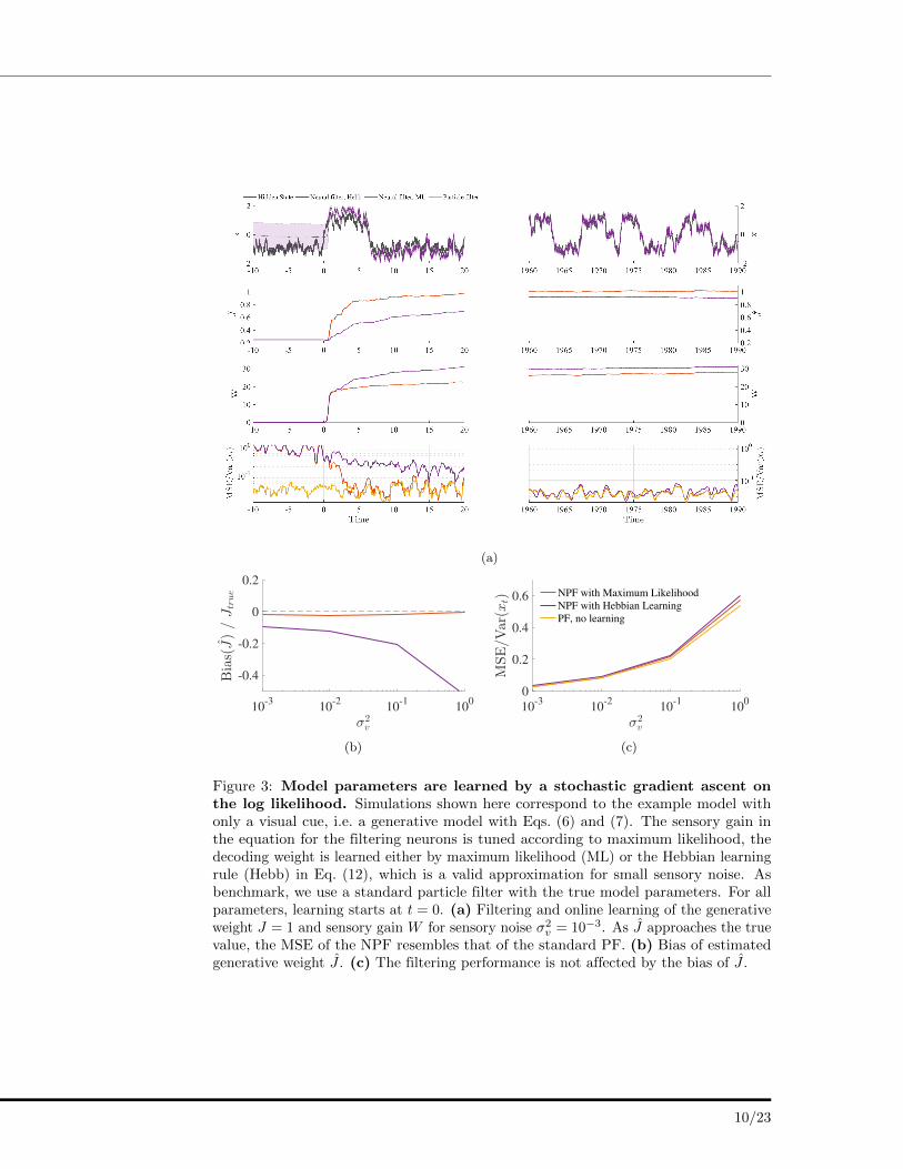
We illustrate the learning of generative model parameters using our example (seeMethods and S1 Appendix for details). This time, the frog only relies on his visualchannel vt, but in addition to tracking the insect, he also has to learn the generativefactor J in the function g(x) = Jx, which relates the position of the insect to the visual

input. Simultaneously, it also learns the gain W(v)t and with that implicitly an estimate

of the reliability of its visual input. Figure 3 shows that this identification problem canbe solved efficiently by the NPF, with an MSE that gradually approaches that of thebenchmark (a standard PF with the ground-truth parameters) as the estimate of theparameters get more accurate (Fig. 3a). We find this to be true over a wide range ofobservation noise σ2

v . Values of the estimator J , i.e. the learned value of the generativefactor, tend to exhibit a slight negative bias, but for an observation noise of up toΣy = 0.1 still stay in a 2%-region below the true generative weight.

It is noteworthy that the learning rule for the generative factor J can be simplifiedsubstantially for small observation noise:

η−1J ∆J ≈ 〈(dvt − Jz(i)t dt) · z(i)t 〉. (12)

Our findings suggest that this learning rule, which we will refer to as ‘Hebbian’ forreasons we illustrate below, leads to an estimator J for the generative weight J which isslightly negatively biased across initial conditions (Fig. 3c). The absolute value of thisbias decreases for smaller observation noise Σy and the learning rule in Eq. (12)becomes exact for Σy → 0. Moreover, this bias does not seem to affect the filteringperformance as measured by the MSE (Fig. 3b).

Neuronal Implementation

Recurrent neuronal dynamics In our example, we have interpreted the NPF as

the neuronal dynamics of a population of N × n filter neurons z(i)t , whose neuronal

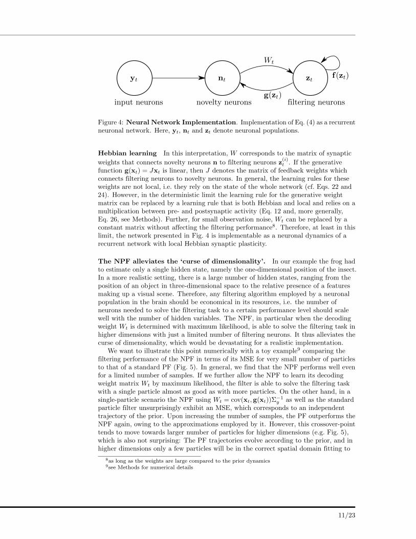
activities represent samples of the posterior, which is in line with the neural samplinghypothesis [33]. Thus, analog neuronal activities are identified with the continuousparticle state, for instance in terms of their instantaneous firing rate. The internaldynamics, or self interaction, of the filtering neurons is governed by the nonlinearfunction f(zt), which incorporates prior knowledge as a state-dependent leak. Inaddition, they are recurrently connected to populations of novelty neurons nt via thefeedforward synaptic weights Wt and feedback connections whose strength is governedby the nonlinearity g(zt). The dynamics of the novelty neurons are governed by theinnovation term dnt = dyt − g(zt) dt. As input to this network we consider a neuronalpopulation yt whose rates are evoked from the underlying hidden stimulus xt via thegenerative dynamics in Eq. (2) (Fig. 4).

9/23

(a)

10-3

10-2

10-1

100

σ2v

-0.4

-0.2

0

0.2

Bias(J)/Jtrue

(b)

10-3

10-2

10-1

100

σ2v

0

0.2

0.4

0.6

MSE/V

ar(x

t) NPF with Maximum Likelihood

NPF with Hebbian LearningPF, no learning

(c)

Fig 3: Model parameters are learned by a stochastic gradient ascent on thelog likelihood. Simulations shown here correspond to the example model with only avisual cue, i.e. a generative model with Eqs. (6) and (7). The sensory gain in the equationfor the filtering neurons is tuned according to maximum likelihood, the decoding weightis learned either by maximum likelihood (ML) or the Hebbian learning rule (Hebb) inEq. (12), which is a valid approximation for small sensory noise. As benchmark, we usea standard particle filter with the true model parameters. For all parameters, learningstarts at t = 0. (a) Filtering and online learning of the generative weight J = 1 andsensory gain W for sensory noise �2

v = 10�3. As J approaches the true value, the MSEof the NPF resembles that of the standard PF. (b) Bias of estimated generative weightJ . (c) The filtering performance is not affected by the bias of J .

PLOS 11/23

Figure 3: Model parameters are learned by a stochastic gradient ascent onthe log likelihood. Simulations shown here correspond to the example model withonly a visual cue, i.e. a generative model with Eqs. (6) and (7). The sensory gain inthe equation for the filtering neurons is tuned according to maximum likelihood, thedecoding weight is learned either by maximum likelihood (ML) or the Hebbian learningrule (Hebb) in Eq. (12), which is a valid approximation for small sensory noise. Asbenchmark, we use a standard particle filter with the true model parameters. For allparameters, learning starts at t = 0. (a) Filtering and online learning of the generativeweight J = 1 and sensory gain W for sensory noise σ2

v = 10−3. As J approaches the truevalue, the MSE of the NPF resembles that of the standard PF. (b) Bias of estimatedgenerative weight J . (c) The filtering performance is not affected by the bias of J .

10/23

yt nt zt

Wt

g(zt)

f(zt)

input neurons novelty neurons filtering neurons

Fig 4: Neural Network Implementation. Implementation of Eq. (4) as a recurrentneuronal network. Here, yt, nt and zt denote neuronal populations.

1 2 4 8 16 32 64 128

Number of particles

10-1

100

MSE

/Tr(Σ

prior)

NPFNPF with Maximum LikelihoodPF

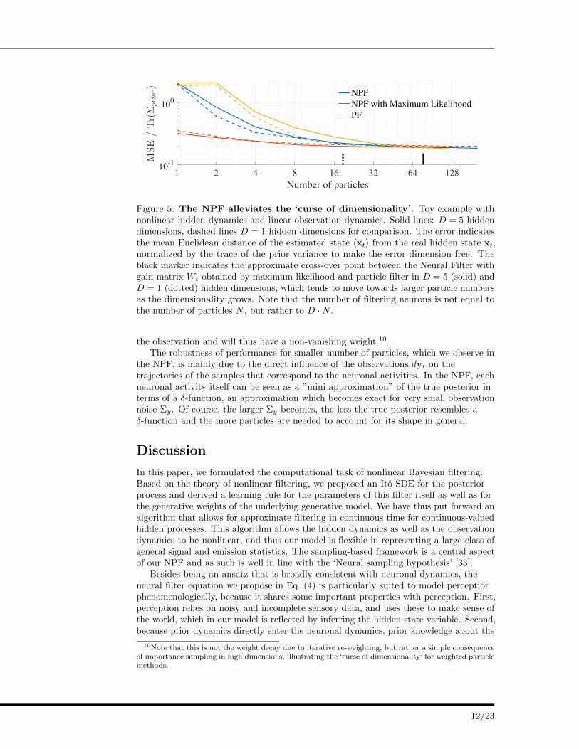
Fig 5: The NPF alleviates the ‘curse of dimensionality’. Toy example withnonlinear hidden dynamics and linear observation dynamics. Solid lines: D = 5 hiddendimensions, dashed lines D = 1 hidden dimensions for comparison. The error indicatesthe mean Euclidean distance of the estimated state hxti from the real hidden state xt,normalized by the trace of the prior variance to make the error dimension-free. Theblack marker indicates the approximate cross-over point between the Neural Filter withgain matrix Wt obtained by maximum likelihood and particle filter in D = 5 (solid) andD = 1 (dotted) hidden dimensions, which tends to move towards larger particle numbersas the dimensionality grows. Note that the number of filtering neurons is not equal tothe number of particles N , but rather to D · N .

for a limited number of samples. If we further allow the NPF to learn its decoding 299

weight matrix Wt by maximum likelihood, the filter is able to solve the filtering task 300

with a single particle almost as good as with more particles. On the other hand, the 301

NPF using Wt = cov(xt,g(xt))⌃�1y as well as the standard particle filter unsurprisingly 302

exhibit an MSE, which corresponds to an independent trajectory of the prior. Upon 303

increasing the number of samples, the PF outperforms the NPF again, owing to the 304

approximations employed by it. However, this crossover-point tends to move towards 305

larger number of particles for higher dimensions (e.g. Fig. 5), which is also not 306

surprising: The PF trajectories evolve according to the prior, and in higher dimensions 307

only a few particles will be in the correct spatial domain fitting to the observation and 308

will thus have a non-vanishing weight.10. 309

The robustness of performance for smaller number of particles, which we observe in 310

the NPF, is mainly due to the direct influence of the observations dyt on the 311

trajectories of the samples that correspond to the neuronal activities. In the NPF, each 312

neuronal activity itself can be seen as a ”mini approximation” of the true posterior in 313

terms of a �-function, an approximation which becomes exact for very small observation 314

noise ⌃y. Of course, the larger ⌃y becomes, the less the true posterior resembles a 315

�-function and the more particles are needed to account for its shape in general. 316

10Note that this is not the weight decay due to iterative re-weighting, but rather a simple consequenceof importance sampling in high dimensions, illustrating the ‘curse of dimensionality’ for weighted particlemethods.

PLOS 12/23

Figure 4: Neural Network Implementation. Implementation of Eq. (4) as a recurrentneuronal network. Here, yt, nt and zt denote neuronal populations.

Hebbian learning In this interpretation, W corresponds to the matrix of synaptic

weights that connects novelty neurons n to filtering neurons z(i)t . If the generative

function g(xt) = Jxt is linear, then J denotes the matrix of feedback weights whichconnects filtering neurons to novelty neurons. In general, the learning rules for theseweights are not local, i.e. they rely on the state of the whole network (cf. Eqs. 22 and24). However, in the deterministic limit the learning rule for the generative weightmatrix can be replaced by a learning rule that is both Hebbian and local and relies on amultiplication between pre- and postsynaptic activity (Eq. 12 and, more generally,Eq. 26, see Methods). Further, for small observation noise, Wt can be replaced by aconstant matrix without affecting the filtering performance8. Therefore, at least in thislimit, the network presented in Fig. 4 is implementable as a neuronal dynamics of arecurrent network with local Hebbian synaptic plasticity.

The NPF alleviates the ‘curse of dimensionality’. In our example the frog hadto estimate only a single hidden state, namely the one-dimensional position of the insect.In a more realistic setting, there is a large number of hidden states, ranging from theposition of an object in three-dimensional space to the relative presence of a featuresmaking up a visual scene. Therefore, any filtering algorithm employed by a neuronalpopulation in the brain should be economical in its resources, i.e. the number ofneurons needed to solve the filtering task to a certain performance level should scalewell with the number of hidden variables. The NPF, in particular when the decodingweight Wt is determined with maximum likelihood, is able to solve the filtering task inhigher dimensions with just a limited number of filtering neurons. It thus alleviates thecurse of dimensionality, which would be devastating for a realistic implementation.

We want to illustrate this point numerically with a toy example9 comparing thefiltering performance of the NPF in terms of its MSE for very small number of particlesto that of a standard PF (Fig. 5). In general, we find that the NPF performs well evenfor a limited number of samples. If we further allow the NPF to learn its decodingweight matrix Wt by maximum likelihood, the filter is able to solve the filtering taskwith a single particle almost as good as with more particles. On the other hand, in asingle-particle scenario the NPF using Wt = cov(xt,g(xt))Σ

−1y as well as the standard

particle filter unsurprisingly exhibit an MSE, which corresponds to an independenttrajectory of the prior. Upon increasing the number of samples, the PF outperforms theNPF again, owing to the approximations employed by it. However, this crossover-pointtends to move towards larger number of particles for higher dimensions (e.g. Fig. 5),which is also not surprising: The PF trajectories evolve according to the prior, and inhigher dimensions only a few particles will be in the correct spatial domain fitting to

8as long as the weights are large compared to the prior dynamics9see Methods for numerical details

11/23

yt nt zt

Wt

g(zt)

f(zt)

input neurons novelty neurons filtering neurons

Fig 4: Neural Network Implementation. Implementation of Eq. (4) as a recurrentneuronal network. Here, yt, nt and zt denote neuronal populations.

1 2 4 8 16 32 64 128

Number of particles

10-1

100

MSE

/Tr(Σ

prior)

NPFNPF with Maximum LikelihoodPF

Fig 5: The NPF alleviates the ‘curse of dimensionality’. Toy example withnonlinear hidden dynamics and linear observation dynamics. Solid lines: D = 5 hiddendimensions, dashed lines D = 1 hidden dimensions for comparison. The error indicatesthe mean Euclidean distance of the estimated state hxti from the real hidden state xt,normalized by the trace of the prior variance to make the error dimension-free. Theblack marker indicates the approximate cross-over point between the Neural Filter withgain matrix Wt obtained by maximum likelihood and particle filter in D = 5 (solid) andD = 1 (dotted) hidden dimensions, which tends to move towards larger particle numbersas the dimensionality grows. Note that the number of filtering neurons is not equal tothe number of particles N , but rather to D · N .

for a limited number of samples. If we further allow the NPF to learn its decoding 299

weight matrix Wt by maximum likelihood, the filter is able to solve the filtering task 300

with a single particle almost as good as with more particles. On the other hand, the 301

NPF using Wt = cov(xt,g(xt))⌃�1y as well as the standard particle filter unsurprisingly 302

exhibit an MSE, which corresponds to an independent trajectory of the prior. Upon 303

increasing the number of samples, the PF outperforms the NPF again, owing to the 304

approximations employed by it. However, this crossover-point tends to move towards 305

larger number of particles for higher dimensions (e.g. Fig. 5), which is also not 306

surprising: The PF trajectories evolve according to the prior, and in higher dimensions 307

only a few particles will be in the correct spatial domain fitting to the observation and 308

will thus have a non-vanishing weight.10. 309

The robustness of performance for smaller number of particles, which we observe in 310

the NPF, is mainly due to the direct influence of the observations dyt on the 311

trajectories of the samples that correspond to the neuronal activities. In the NPF, each 312

neuronal activity itself can be seen as a ”mini approximation” of the true posterior in 313

terms of a �-function, an approximation which becomes exact for very small observation 314

noise ⌃y. Of course, the larger ⌃y becomes, the less the true posterior resembles a 315

�-function and the more particles are needed to account for its shape in general. 316

10Note that this is not the weight decay due to iterative re-weighting, but rather a simple consequenceof importance sampling in high dimensions, illustrating the ‘curse of dimensionality’ for weighted particlemethods.

PLOS 12/23

Figure 5: The NPF alleviates the ‘curse of dimensionality’. Toy example withnonlinear hidden dynamics and linear observation dynamics. Solid lines: D = 5 hiddendimensions, dashed lines D = 1 hidden dimensions for comparison. The error indicatesthe mean Euclidean distance of the estimated state 〈xt〉 from the real hidden state xt,normalized by the trace of the prior variance to make the error dimension-free. Theblack marker indicates the approximate cross-over point between the Neural Filter withgain matrix Wt obtained by maximum likelihood and particle filter in D = 5 (solid) andD = 1 (dotted) hidden dimensions, which tends to move towards larger particle numbersas the dimensionality grows. Note that the number of filtering neurons is not equal tothe number of particles N , but rather to D ·N .

the observation and will thus have a non-vanishing weight.10.The robustness of performance for smaller number of particles, which we observe in

the NPF, is mainly due to the direct influence of the observations dyt on thetrajectories of the samples that correspond to the neuronal activities. In the NPF, eachneuronal activity itself can be seen as a ”mini approximation” of the true posterior interms of a δ-function, an approximation which becomes exact for very small observationnoise Σy. Of course, the larger Σy becomes, the less the true posterior resembles aδ-function and the more particles are needed to account for its shape in general.

Discussion

In this paper, we formulated the computational task of nonlinear Bayesian filtering.Based on the theory of nonlinear filtering, we proposed an Ito SDE for the posteriorprocess and derived a learning rule for the parameters of this filter itself as well as forthe generative weights of the underlying generative model. We have thus put forward analgorithm that allows for approximate filtering in continuous time for continuous-valuedhidden processes. This algorithm allows the hidden dynamics as well as the observationdynamics to be nonlinear, and thus our model is flexible in representing a large class ofgeneral signal and emission statistics. The sampling-based framework is a central aspectof our NPF and as such is well in line with the ‘Neural sampling hypothesis’ [33].

Besides being an ansatz that is broadly consistent with neuronal dynamics, theneural filter equation we propose in Eq. (4) is particularly suited to model perceptionphenomenologically, because it shares some important properties with perception. First,perception relies on noisy and incomplete sensory data, and uses these to make sense ofthe world, which in our model is reflected by inferring the hidden state variable. Second,because prior dynamics directly enter the neuronal dynamics, prior knowledge about the

10Note that this is not the weight decay due to iterative re-weighting, but rather a simple consequenceof importance sampling in high dimensions, illustrating the ‘curse of dimensionality’ for weighted particlemethods.

12/23

environment is automatically incorporated and can in principle be learned. Third,information from different sensory modalities is efficiently combined as a weighted inputto the population of filtering neurons. Lastly, perception can adapt to changes in theenvironment, which is taken into account by a dynamical gain and online parameterupdates.

The implementation on a biologically realistic architecture imposes constraints onthe algorithm itself as well as on how we can interpret its elements and structure. Weshould always be aware that these constraints describe a highly simplified version of thereal biological underpinning, but have successfully been applied in network models toqualitatively understand core computations in the brain [36, p. 229ff]. First, neuronscommunicate among each other via discrete spikes, i.e. a digital signal. In contrast, weuse the term ‘neuronal activity’ to denote an analog quantity. In some cases, for instancefor a large number of neurons [36, p. 231], this ‘analog quantity’ may for instancecorrespond to an instantaneous firing rate. To take into account ‘negative’ neuronalactivities, we could also consider deviations from a baseline firing rate or the membranepotential of the neuron, or the logarithm of the firing rate. Secondly, computations inand between neurons are performed through a weighted sum of inputs from cells theyare connected to, and these inputs may be a (nonlinear) transformation of thepresynaptic activity. Third, a hallmark of neural circuits is the synaptic connectivitybetween the neurons, the connection strength of which quantified by connective weights.These synaptic weights are modified by learning rules, which in the most simple case arelocal, i.e. they depend on the pre- and the postsynaptic neuronal activity. The learningrules in our model are in general not local, and in fact, each filter neuron z(k) has toknow about the state of every other filter neuron and/or novelty neuron. Apart fromthat, when parameters are learned online, it is not clear how the filter derivative shouldbe implemented in the network. However, we have shown that the learning rules of ourmodel become both Hebbian and local for small observation noise, making theselearning rules biologically plausible in this limit. Lastly, because the number of neuronsin the brain is finite, computations clearly have to rely on a finite number of neurons, afact we are taking into account by representing probability distributions with samples.Because these requirements are met by our proposed network structure, we consider ourneuronal dynamics for filtering to be in line with standard network models.

Comparison to related work

The NPF is a filtering algorithm for a continuous-time continuous-state generativemodel with nonlinear hidden and observation dynamics. Filtering algorithms based onlinear generative models have been subject to extensive research. and mainly study howthe analytical solution to this problem, the Kalman filter, can be implemented withneurons (e.g. [11, 12,31,37]). However, the posterior resulting from a Kalman filter isalways Gaussian, which is highly restrictive and does not properly reflect activitydistributions observed in neurons (compare for instance the observations related tosparse coding as in [38]). Unlike the various extensions of the Kalman filter [13] – suchas the EKF or the unscented Kalman filter [39] – which are applied to nonlinearsystems, the NPF is not restricted to approximate the posterior by a Gaussianparametrized by its first and second moment. Rather, due to the nonlinearity in thenetwork dynamics it may represent any probability distribution at any given time step.

An important aspect of our work is the sampling-based representation of probabilitydistributions, whereby the activity of each neuron is considered a single sample. Thereare two main competing proposals about how the probability distributions underlyingBayesian computations might be represented in the brain. Firstly, it has been suggestedthat probability distributions are expressed as probabilistic population codes(PPC [40]), in which each neuron represents a state of the encoded random variable and

13/23

their activities are proportional to the probability of the corresponding state. Filteringapproaches based on population codes, in which the neuronal activity directly relates tothe posterior or the log posterior, have been explored in the literature for a large set ofmodels, e.g. [11, 12,41,42]. In this representation, neurons directly correspond to theparameters of the distribution, and thus the critical factor for accuracy is the number ofneurons. Further, they all suffer from the ‘curse of dimensionality’ for multimodaldistribution. The second proposal, called neural sampling hypothesis [33], uses aninference scheme where the activity of each neuron represents a sample from theunderlying probability distribution. Since our filtering algorithm is based on unweightedsamples, our findings are in line with the advantages of the sampling-basedrepresentation outlined in [33]: it can represent any distribution without the need for aparametric form, it mitigates the ‘curse of dimensionality’ and it is well-suited forlearning. Filtering approaches implementing Markov-chain Monte Carlo (MCMC)algorithms have received some attention lately [43, 44], but since they rely on a discretestate space and assume a different coding scheme than the one suggested in [33], theadvantages listed there do not necessarily emerge from these models.

As a filtering algorithm, the NPF is well in accordance with existing sample-basedfiltering approaches. Our ansatz may be seen as a particle filter where all particles carrythe same weight and which, therefore, avoids numerical pitfalls such as weightdegeneracy. This problem is notorious in standard MCMC particle filters [18] andbecomes even more severe as the number of hidden dimensions grows. The curse ofdimensionality, i.e. the exponential growth of approximation error with the dimension ofthe underlying model, is an inevitable nuisance in standard MCMC approaches. Thereare some tricks to deal with these problems, for instance by particle resampling or usinga more refined propagator for the particles (like the optimal importance functionin [18]), but neither solution is able to properly circumvent weight decay in general.Moreover, there is currently no proposed implementation of weighted particle methodsin a neural architecture. For instance, the need to renormalize the weights at each timestep introduces a coupling between the particles: While their trajectories areindependent, their weights are certainly not. On the other hand, the neural filter, notrelying on importance weights in the first place, does not suffer from these numericalpitfalls and their related implementational issues. The curse of dimensionality seems tobe avoided, or at least mitigated, by the fact that the observations directly enter theparticle trajectories. However, the particles following the NPF dynamics are notcompletely independent either. Coupling between the particles is mediated by thedecoding weight matrix Wt, whose learning rule is influenced by all the particles. Thiscould be avoided by fixing Wt to a constant consistent with observational noise Σy,e.g. after learning. Even if it is numerically a bit off what we think the ‘real’ decodingweight should be, the filtering performance is not seriously affected and particletrajectories are effectively decoupled.

In the literature, there have been other approaches for particle filtering withoutimportance weights, derived rigorously from mathematical filtering theory [45,46]. Oneof these approaches, the so-called feedback particle filter [45], is based on a similar SDEfor the particle trajectories as the one we propose in Eq. (4). It can be shown that theunderlying distribution of the feedback particle filter evolves exactly according to theKushner equation, whereas our approach merely approximates it. However, thecomputation of the gain function in the feedback particle filter needs access to the fullfiltering distribution itself, and in order to avoid numerical issues their algorithm relieson a regularization scheme that would be hard to justify biologically. Though formally amultivariate version of the feedback particle filter exists, the gain function cannot besolved for in closed form. The Neural Filter, though not an exact particle algorithm,overcomes this drawback by being readily applicable in higher dimensions and by being

14/23

comparatively easy to compute.The neuronal network structure (Fig. 4) we propose to implement the neuronal

dynamics according to Eq. (4) is structurally similar to the one proposed in [9]. As intheir model, we represent neuronal activities in terms of their instantaneous firing rate,which is an approximation to the spiking nature of biological neurons. In theirpredictive coding model, a central role is assigned to the predictive error signal, whichcan be compared to the dynamics of the novelty neurons or novelty signal dnt in ourmodel. Accordingly, equations for the neuronal dynamics and for learning thegenerative weight in the small observation noise limit is structurally similar. However,our model generalizes the one in [9] in the sense that we allow dynamics in the prior,which is directly reflected in the dynamics of the filtering neurons.

Implications

The three central aspects of our work, namely a sampling-based representation, afiltering algorithm with adaptive gain and the structure of the recurrent neuronalnetwork, result in the following implications for the neuronal network:

1. The network is robust against neuronal failure.

2. An internal model about the world becomes manifest in internal neuronaldynamics

3. Neuronal variability is tuned according to sensory reliability.

4. Neurons may code for the novelty given by discrepancy between prediction by aninternal model and actual observations.

The first implication follows directly from the sampling-based representation, namelyrobustness against neuronal failure. For example, if a distribution is represented by 1000particles, removing 10% will not significantly decrease the ability of the other particlesto represent the probability distribution. In an extreme case, we could consider a singleneuron to represent the whole distribution, given that its activity state can take valuesin the same range as the hidden state and we allow it to sample the distribution in time.Apart from that, as we have seen numerically, the ability to perform filtering with areduced number of particles is not affected by particle removal to a large extent either,at least not in the particular algorithm we propose. However, some degree of plasticityor rewiring would be necessary in order to read out expectations from the decimatedneuronal population. On the other hand, in parametric representations such as a PPC,where each neuron determines the height of a particular tuning curve assigned to it andthat actually rely on the tuning curves to cover the space densely [40], neuronal failurecan be devastating: With each neuron that breaks down, a particular point in statespace cannot be represented directly anymore. Clearly, a single neuron would never beable to account for any other distribution than the one resembling its own tuning curve.

The second and third implication is a consequence of the adaptive gain, i.e. thedecoding weight Wt, that determines the emphasis that is laid on new observations. Aswe have demonstrated, the gain Wt in our model increases with sensory reliability bothaccording to sensory noise and ambiguity in the input generation, putting moreemphasis on the observations versus its internal model. In the absence of observations,observation noise is maximal and the neuronal dynamics follow those of the hidden statewhich comprises an internal model about the world. With availability of observations,sensory reliability naturally increases and variability across samples should decrease,because now their dynamics are influenced by the same stimulus via the gain Wt.Indeed, it has been found that spontaneous neuronal activities relate to prior

15/23

expectations about a stimulus in visual cortex [32]. Further, it has been shown thatinter-trial variability of neuronal responses declines upon stimulus onset [7]. Both theseexperimental findings are nicely in line with our theoretical predictions.

Conclusion and Outlook

With the Neural Particle Filter we have come up with an algorithm that allows neuronsto perform nonlinear Bayesian filtering in a sampling-based manner. Specifically, theneuronal implementation is based on a network of recurrently connected analog neuronswhose dynamics are governed by the NPF algorithm. In future work, the biologicalplausibility of this recurrent network model will be further addressed. First, observingthat the learning rules in general, i.e. for nonvanishing observation noise, do not fulfillthe requirement of locality, which is needed for a biologically plausible learning rule (e.g.a Hebbian learning rule), the model could be enhanced such that individual filteringneurons obey different rather than identical dynamics. We could for instance considerN different subnetworks and locally determine the weights in these subnetworks,possibly taking into account a (slowly-changing) global modulation factor. Such anapproach would also effectively decouple the particles on a smaller timescale. Second,by including the theory of filtering and identification of point processes, our algorithmcould be extended such that a spike-based representation may be accounted for.

Methods

Details on numerical experiments

The choice of the decoding weight Wt

In our numerical simulations, we consider and compare two choices of the decodingweight Wt, which we will quickly motivate here.

As a first choice, we consider Wt = cov(x,g(x)T )Σ−1y , a choice inspired by the

dynamics of the formal solution. In particular, consider the dynamics of the firstposterior moment11, which by comparison with the NPF equation (Eq. 4) directlymotivates this particular choice of the decoding weights. Thereby, the covariance

cov(x,g(x)T ) is estimated empirically from the samples z(k)t via

cov(x,g(x)) ≈ 1

N

N∑k=1

z(k)t g(z

(k)t )T − 1

N2

N∑k,l=1

z(k)t g(z

(l)t )T . (13)

As a second choice, we consider W = WML, i.e. the decoding weight Wt and thus theNeural Filter itself is tuned via maximum likelihood. The learning rule is given inEq. (22) and corresponds to an online update of the decoding weight at each time step.What is peculiar about this choice is that here a decoding rather than a generativemodel parameter is learned, illustrating that inference and learning can be veryintertwined: In fact, it is actually possible to rephrase the filtering problem in terms of alearning problem by giving an ansatz for a decoder whose parameters have to be learnedsuch that it can perform filtering, but we will not consider this rather extreme case here.

11see S1 Appendix

16/23

Dynamics and parameters

For our simulations, we use a nonlinear hidden dynamics, that was chosen to have abimodal stationary distribution:

dxt = axt(b− x2t ) dt+ σxdωt. (14)

The parameters a > 0 and b > 0 can be used to tune the shape of the bimodaldistribution, whereby the positions of the two modes is determined by ±b and a defineshow sharply the distribution is peaked around the modes. Unless stated otherwise,parameters for the deterministic dynamics were a = 3 and b = 1, resulting in a bimodaldistribution with distinct, but not too sharp peeks at ±1, such that it is possible for thehidden state to switch from one mode to the other.

In our examples in Fig. 1, we employ both linear and sigmoid observation dynamicsg(x), thereby simulating multisensory integration with our model (cf. Eqs. 8 and 7). Forthe plots in Fig. 2, we use only one sensory modality per row. The observation noise σvand σa is varied between 10−4 and 300.

In the multidimensional simulations in Fig. 5, the hidden dynamics within eachdimension is independent of the other dimensions and and corresponds to Eq. (14), withΣx chosen to be the unit matrix. The stationary distribution of this dynamics is thus amultimodal distribution with 2n peaks for n dimensions. The linear generative functionis given by g(x) = Jx with J a rotation matrix rotating the hidden state vector by 30degrees around each spatial axis. In the simulations shown in Fig. 5, Σy = 0.1 · I.

Mean-squared errors (MSE) and biases of estimated quantities or parameters θ werecomputed by

MSE =1

T

T∑t=1

|xt − 〈x〉|2, (15)

Bias(θ) =1

T

T∑t=1

θt − θt, (16)

where θt denotes the true or benchmark (particle filter) value. Unless stated otherwise,MSEs are normalized with respect to the trace of the stationary prior variance Σprior tomake performance comparable and, if needed, independent of the number of hiddendimensions.

Other simulation parameters comprise the time step size, which was set todt = 0.005 throughout all simulations. All simulations were run for 500’000 time steps,corresponding to 2500 time units. Unless stated otherwise, MSEs and biases wereaveraged over the last 1000 time units, equaling 200’000 time steps.

Benchmark models

We would like to stress that the generative model we chose in our examples arenonlinear both in prior as well as in observation dynamics. This implies that a closedform solution to this problem does not exist, and thus approximations have to beemployed. Therefore, when assessing the performance of the NPF, we compare it to twoapproximate filtering algorithms, both of which widely used in approximating theposterior distribution in nonlinear filtering problems: a standard particle filter [18] andcontinuous-time version of the extended Kalman filter [26]. For further information onthese algorithms, see S1 Appendix.

17/23

Maximum likelihood parameter learning

The cost function

For the continuous-time continuous state-space generative model given by Eqs. (1) and(2), learning in the mathematical literature commonly referred to as ‘systemidentification’, is a tough problem which has hardly been looked at. In fact, the (to ourknowledge) only reference which gives an explicit cost function for identification in oursetting is a technical report by Moura and Mitter [47]. Based on a change of probabilitymeasure, they propose a cost function that is equivalent to the log likelihood of theinput log pθ(Yt) with model parameters θ, which for our model reads:

Lofflinet (θ) =

∫ t

0

〈g(xs)〉TΣ−1y dys −

1

2〈g(xs)〉TΣ−1

y 〈g(xs)〉 ds, (17)

where expectations are taken with respect to the filtering distribution at time s,p(xs|Ys).

In a discrete-time approximation, Eq. (17) immediately suggests an onlinemaximization scheme. Instead of maximizing the cost function at a time t for the wholeobservation sequence Yt, implying we would have to run the filter all over again eachtime we change the parameters, we just perform a gradient ascent with respect to theparameters θ on the last contribution to the integral, i.e. to

Lonlinet (θ) = 〈g(xt)〉TΣ−1

y dyt −1

2〈g(xt)〉TΣ−1

y 〈g(xt)〉 dt, (5)

where expectations are with respect to the filtering distribution at time t, p(xt|Yt). Itcan be shown that maximization of this cost function is equivalent to a minimization ofthe reconstruction error (dyt − g(xt) dt)

2 at each time step (see S1 Appendix for aproof).

Learning rules

Parameter learning is implemented by maximizing the log likelihood (Eq. 5) by agradient ascent with respect to the model parameters θ, giving rise to the followingonline learning rule for the parameters:

η−1θ ∆θ =

( ∂∂θ〈g(xt)〉

)TΣ−1y

(dyt − 〈g(xt)〉 dt

). (18)

This approximation of learning is justified if the time scale of learning is much largerthan the dynamics of the filter, i.e. for small learning rates.

Equation (18) exhibits a peculiar structure: The novelty signal dyt − 〈g(xt)〉 dt ismultiplied with a parameter gradient on the posterior estimate of the generativefunction 〈g(xt)〉. Thus, we have to take into account the implicit change of the posteriordistribution, the so called filter derivative, with respect to the model parameters. Thefilter derivative is in general hard or even impossible to compute analytically and manyidentification problems deal with estimating it (cf. for instance [19,35]).

In our model, we make use of the approximated posterior dynamics in order toderive dynamics of the filter derivative for parameter learning. Equation 18 can beapproximated by taking N samples from the NPF equation (4) in order to express theposterior estimates:

〈g(xt)〉 ≈1

N

N∑k=1

g(z(k)t ), (19)

∂

∂θ〈g(xt)〉 ≈

1

N

N∑k=1

G(z(k)t )

∂z(k)t

∂θ, (20)

18/23

where Gij(z(k)) = ∂gi

∂xj(z(k)) denotes the Jacobian of the generative function. Thus, the

filter derivative is taken into account by considering the infinitesimal change in theposition of sample z(k) with respect to the change in parameter value θ.

The single particle filter derivative,∂x

(k)t

∂θ , cannot be computed directly. However,based on Eq. (4), it is possible to compute its dynamics:

d

(∂z

(k)t

∂θ

)=

∂

∂θ

(dz

(k)t

). (21)

Note that every single parameter that is learned has N accompanying filter derivativesof this form.

In this work we are interested in learning the decoding weight matrix Wt and, for alinear observation dynamics g(x) = Jx, in learning the generative matrix J, respectively.The resulting learning rules for the components of the decoding weight matrix withlearning rate ηW are given by

∆Wij = ηW∂

∂Wij

〈g(xt)〉TΣ−1y (dyt − 〈g(xt)〉dt) , (22)

with filter derivative dynamics

d

(∂z

(k)t

∂Wij

)=

(F (z

(k)t )−WG(z

(k)t )) ∂z(k)t

∂Wijdt+

[dyt − g(z

(k)t )dt

]jei, (23)

where Fij(z(k)) = ∂fi

∂xj(z(k)) denotes the Jacobian of the nonlinear hidden dynamics and

ei denotes the unit vector in the i-th direction. This implies that, when we take Wt tobe a plastic decoding weight matrix that is learned as observations become available, atleast three equations are needed to infer the hidden state at each time step: First,Eq. (4) to evolve the states of the filter neurons, and second, Eqs. (22) and (23) toupdate the weights in the filter equation.

Analogously, learning rules for the components of the generative matrix for linearobservation dynamics g(x) = Jx read

∆Jij = ηJ

[(∂〈xt〉∂Jij

)TJTΣ−1

y (dyt − J〈xt〉 dt) +(

Σ−1y (dyt − J〈xt〉 dt)

)ij

].(24)

In addition to a term proportional to the filter derivative, the learning rule contains asecond term that emerges from an explicit dependence of the likelihood in thegenerative weight. Filter derivatives are given by

d

(∂z

(k)t

∂Jij

)=

(F (z

(k)t )−WJ

) ∂z(k)t

∂Jijdt− x(k)t,jWeidt. (25)

Bias due to sampling In the derivation of these learning rules, we used asampling-based representation of the approximated posterior in order to estimatelog-likelihood and gradients. This introduces a bias in these estimations, which weshould correct for when computing parameter estimates. Unfortunately, this bias is ingeneral not analytically accessible, but at least for a linear generative model it can beshown that it vanishes with 1/N (for a proof, see S1 Appendix).

19/23

Approximation for small observation noise The learning rules we obtain for thedecoding weights Wt and the generative weights J are not local, implying that theweights can only be computed when knowing the state of each filter neuron at each time.However, for small observation noise the learning rule for the generative weight J canbe approximated by a local learning rule with a Hebbian structure. First, we canneglect the filter derivative, which decays to zero very fast because in this limit, thedecoding weight Wt is generally large (cf. Eq. 25), and thus the first term in Eq. (24)vanishes. Second, because in this limit the posterior will approach a δ-distributionaround the true hidden state x, as does the approximated posterior, we canapproximate the learning rule for J by:

η−1J ∆J ∝ (dyt − J〈xt〉 dt)〈xt〉T ≈ 〈(dyt − Jxt)xTt 〉, (26)

which takes the form of a local Hebbian learning rule.

Supporting Information

S1 Appendix. The Neural Particle Filter: Mathematical Appendix.

References

1. Knill DC, Pouget A. The Bayesian brain: the role of uncertainty in neural codingand computation. Trends in Neurosciences. 2004;27(12):712–719.doi:10.1016/j.tins.2004.10.007.

2. Doya K, Ishii S, Pouget A, Rao RPN. Bayesian Brain: Probabilistic Approachesto Neural Coding. The MIT Press; 2007.

3. Wolpert D, Ghahramani Z, Jordan M. An internal model for sensorimotorintegration. Science. 1995;269(5232):1880–1882. doi:10.1126/science.7569931.

4. Kording KP, Wolpert DM. Bayesian integration in sensorimotor learning. Nature.2004;427(January):244–247. doi:10.1038/nature02169.

5. Ernst MO, Banks MS. Humans integrate visual and haptic information in astatistically optimal fashion. Nature. 2002;415(6870):429–433.doi:10.1038/415429a.

6. Churchland AK, Kiani R, Chaudhuri R, Wang XJ, Pouget A, Shadlen MN.Variance as a signature of neural computations during decision making. Neuron.2011;69(4):818–831. doi:10.1016/j.neuron.2010.12.037.

7. Churchland MM, Yu BM, Cunningham JP, Sugrue LP, Cohen MR, Corrado GS,et al. Stimulus onset quenches neural variability: a widespread corticalphenomenon. Nature Neuroscience. 2010;13(3):369–378. doi:10.1038/nn.2501.

8. Orban G, Berkes P, Fiser J, Lengyel M. Neural Variability and Sampling-BasedProbabilistic Representations in the Visual Cortex. Neuron. 2016;92(2):530–543.doi:10.1016/j.neuron.2016.09.038.

9. Rao RPN, Ballard DH. Predictive coding in the visual cortex: a functionalinterpretation of some extra-classical receptive-field effects. Nature Neuroscience.1999;2(1):79–87. doi:10.1038/4580.

10. Huang Y, Rao RPN. Bayesian Inference and Online Learning in PoissonNeuronal Networks. Neural Computation. 2016;28(8):1503–1526.

20/23

11. Deneve S, Duhamel JR, Pouget A. Optimal sensorimotor integration in recurrentcortical networks: a neural implementation of Kalman filters. The Journal ofneuroscience : the official journal of the Society for Neuroscience.2007;27(21):5744–5756. doi:10.1523/JNEUROSCI.3985-06.2007.

12. Makin JG, Dichter BK, Sabes PN. Learning to Estimate Dynamical State withProbabilistic Population Codes. PLoS Computational Biology. 2015;11(11):1–28.doi:10.1371/journal.pcbi.1004554.

13. Kalman RE. A New Approach to Linear Filtering and Prediction Problems.Transactions of the ASME Journal of Basic Engineering. 1960;82(Series D):35–45.doi:10.1115/1.3662552.

14. Kalman RE, Bucy RS. New Results in Linear Filtering and Prediction Theory.Journal of Basic Engineering. 1961;83(1):95. doi:10.1115/1.3658902.

15. Kording KP, Tenenbaum JB, Shadmehr R. The dynamics of memory as aconsequence of optimal adaptation to a changing body. Nature Neuroscience.2007;10(6):779–786. doi:10.1038/nn1901.

16. Kushner H. On the Differential Equations Satisfied by Conditional ProbabilityDensities of Markov Processes, with Applications. Journal of the Society forIndustrial & Applied Mathematics, Control. 1962;2(1).

17. Zakai M. On the optimal filtering of diffusion processes. Zeitschrift furWahrscheinlichkeitstheorie und verwandte Gebiete. 1969;243.

18. Doucet A, Godsill S, Andrieu C. On sequential Monte Carlo sampling methodsfor Bayesian filtering. Statistics and Computing. 2000;10(3):197–208.doi:10.1023/A:1008935410038.

19. Kantas N, Doucet A, Singh SS, Maciejowski J, Chopin N. On Particle Methodsfor Parameter Estimation in State-Space Models. Statistical Science.2015;30(3):328–351. doi:10.1214/14-STS511.

20. Welling M, Teh YW. Bayesian Learning via Stochastic Gradient LangevinDynamics. In: Proceedings of the 28th International Conference on MachineLearning; 2011.

21. MacKay DJ. Information Theory, Inference and Learning Algorithms. CambridgeUniversity Press; 2005.

22. Hennequin G, Aitchison L, Lengyel M. Fast Sampling-Based Inference inBalanced Neuronal Networks. Advances in Neural Information ProcessingSystems. 2014;.

23. Moreno-Bote R, Knill DC, Pouget A. Bayesian sampling in visual perception.Proceedings of the National Academy of Sciences of the United States of America.2011;108(30):12491–12496. doi:10.1073/pnas.1101430108.

24. Kappel D, Habenschuss S, Legenstein R, Maass W. Network Plasticity asBayesian Inference. PLoS Computational Biology. 2015;11(11):1–31.doi:10.1371/journal.pcbi.1004485.

25. Marr D. Vision - A Computational Investigation into the Human Representationand Processing of Visual Information. WH Freeman & Co. San Francisco; 1982.

21/23

26. Jazwinski AH. Stochastic Processes and Filtering Theory. Bellman R, editor.New York: Academic Press; 1970.

27. Bain A, Crisan D. Fundamentals of Stochastic Filtering. New York: Springer;2009.

28. Doucet A, Johansen A. A tutorial on particle filtering and smoothing: Fifteenyears later. Handbook of Nonlinear Filtering. 2009.

29. Crisan D, Rozovskii B, editors. No Title. 1st ed. Oxford University Press; 2011.

30. Daum F, Huang J. Curse of Dimensionality and Particle Filters. Proceedings ofthe IEEE Aerospace Conference. 2003;4:1979–1993.doi:10.1109/AERO.2003.1235126.

31. Greaves-Tunnell A. An optimization perspective on approximate neural filtering;M.Sc. Thesis, University of Cambridge. 2015.

32. Berkes P, Orban G, Lengyel M, Fiser J. Spontaneous Cortical Activity RevealsHallmarks of an Optimal Internal Model of the Environment. Science.2011;331(6013):83–87. doi:10.1126/science.1195870.

33. Fiser J, Berkes P, Orban G, Lengyel M. Statistically optimal perception andlearning: from behavior to neural representations. Trends in Cognitive Sciences.2010;14(3):119–130. doi:10.1016/j.tics.2010.01.003.

34. Lo JT, Yu L. Recursive neural filters and dynamical range transformers.Proceedings of the IEEE. 2004;92(3):514–535. doi:10.1109/JPROC.2003.823148.

35. Surace SC, Pfister JP. Online Maximum Likelihood Estimation of the Parametersof Partially Observed Diffusion Processes. 2016;(3):1–10.

36. Dayan P, Abbott LF. Theoretical Neuroscience: Computational andMathematical Modeling of Neural Systems. Computational Neuroscience Series.Massachusetts Institute of Technology Press; 2001.

37. Wilson RC, Finkel L. A neural implementation of the Kalman filter. Advances inNeural Information Processing Systems. 2009;22.

38. Olshausen BA, Field DJ. Emergence of simple-cell receptive field properties bylearning a sparse code for natural images. Nature. 1996;381(6583):607–9.doi:10.1038/381607a0.

39. Julier SJ, Uhlmann JK. A New Extension of the Kalman Filter to NonlinearSystems. System Identification. 1997;3:3–2. doi:10.1117/12.280797.

40. Ma WJ, Beck JM, Latham PE, Pouget A. Bayesian inference with probabilisticpopulation codes. Nature neuroscience. 2006;9(11):1432–8. doi:10.1038/nn1790.

41. Beck JM, Pouget A. Exact inferences in a neural implementation of a hiddenMarkov model. Neural computation. 2007;19(5):1344–1361.doi:10.1162/neco.2007.19.5.1344.

42. Sokoloski S. Implementing a Bayes Filter in a Neural Circuit: The Case ofUnknown Stimulus Dynamics. ArXiv. 2015;.

43. Pecevski D, Buesing L, Maass W. Probabilistic inference in general graphicalmodels through sampling in stochastic networks of spiking neurons. PLoSComputational Biology. 2011;7(12). doi:10.1371/journal.pcbi.1002294.

22/23

44. Legenstein R, Maass W. Ensembles of Spiking Neurons with Noise SupportOptimal Probabilistic Inference in a Dynamically Changing Environment. PLoScomputational biology. 2014;10(10):e1003859. doi:10.1371/journal.pcbi.1003859.

45. Yang T, Mehta PG, Meyn SP. Feedback particle filter. IEEE Transactions onAutomatic Control. 2013;58(10):2465–2480. doi:10.1109/TAC.2013.2258825.

46. Crisan D, Xiong J. Approximate McKean–Vlasov representations for a class ofSPDEs. Stochastics An International Journal of Probability and StochasticProcesses. 2010;82(1):53–68. doi:10.1080/17442500902723575.

47. Moura JMF, Mitter SK. Identification and Filtering: Optimal RecursiveMaximum Likelihood Approach; MIT Technical Report. 1986

23/23