Brussels, August 5 2002

Federaal

Sectorale Directie

Planbureau

THE NEW BELGIAN INPUT-OUTPUT TABLE - GENERAL PRINCIPLES

Luc Avonds, Albert Gilot

This paper gives a general outline of the compilation of the input-output table for 1995 bythe Belgian Federal Planning Bureau. It places this compilation in the general frameworkof the ESA 95 national accounts. The emphasis is on the data sources and the compilationmethodology. The different stages in the transition from supply and use tables tosymmetric input-output tables are explained. Much attention is paid to the calculation oftechnical coefficients.

A. Introduction

The input-output table set out below for Belgium refers to the year 1995. It is compiledaccording to the rules of the European system of accounts ESA 19951. It is a part of theintroduction of new national accounts in the member states of the European Community2

that was made compulsory by European regulations. In order to introduce this system:

• a complete new methodology has been worked out

• new data sources have been used

• different institutions are involved in the compilation

This means that the transition from ESA 793 based national accounts to the new ones is notsimply a reform but rather a completely new beginning.

1. EUROSTAT, 11.2. CE, 5.3. EUROSTAT, 9.

Inlichtingen betreffende deze nota kunnen bekomen worden bij Luc Avonds (02/507.74.39, la@plan.be)

Nota

B. An outline of the general framework of the new Belgian national accounts

1. The former situation

1953 was the year covered by the first published national accounts. They were compiledby the National Statistical Institute (NSI)4. The accounting framework used in thesenational accounts was the Standardized system of national accounts of the OEEC5 (fore-runner of the OECD). This system was more or less similar to the first version of theUnited Nations System of National Accounts, the SNA 19536.

The most obvious feature of the underlying statistical system of the national accountswas that it only covered a systematic statistical interrogation of industrial enterprisesand did not include service industries. Production statistics, corresponding to the princi-ples of national accounts, were only created for industrial companies. The calculationsfor service industries were based on partial information gathered from existing statisticsor were simply an extrapolation of an original estimate made for 1953 by means of priceand volume indices7.

In general it can be said that this so-called Traditional Belgian system of nationalaccounts corresponded to the post-war economic reality before the boom of the “goldensixties”. This underlying statistical system and compilation methodology were neverfundamentally changed until the introduction of the ESA 95 with the national accounts-the 1998 version, published in 1999.

The introduction of the ESA 708 and subsequently the ESA 79 accounting systems wasnot accompanied by the introduction of a new underlying statistical system and compi-lation methodology, corresponding to the concepts and definitions of this system. Varia-bles and aggregates initially continued to be still calculated according to the rules of theTraditional system and subsequently

• reclassified according to ESA classifications (NACE/CLIO, COICOP ...)

• adjusted to correspond to ESA concepts and definitions.

4. We do not take into account the earlier “unofficial” estimates made by universities.5. OECE, 18.6. UN, 22.7. INS, 14.8. EUROSTAT, 8.

2

Nota

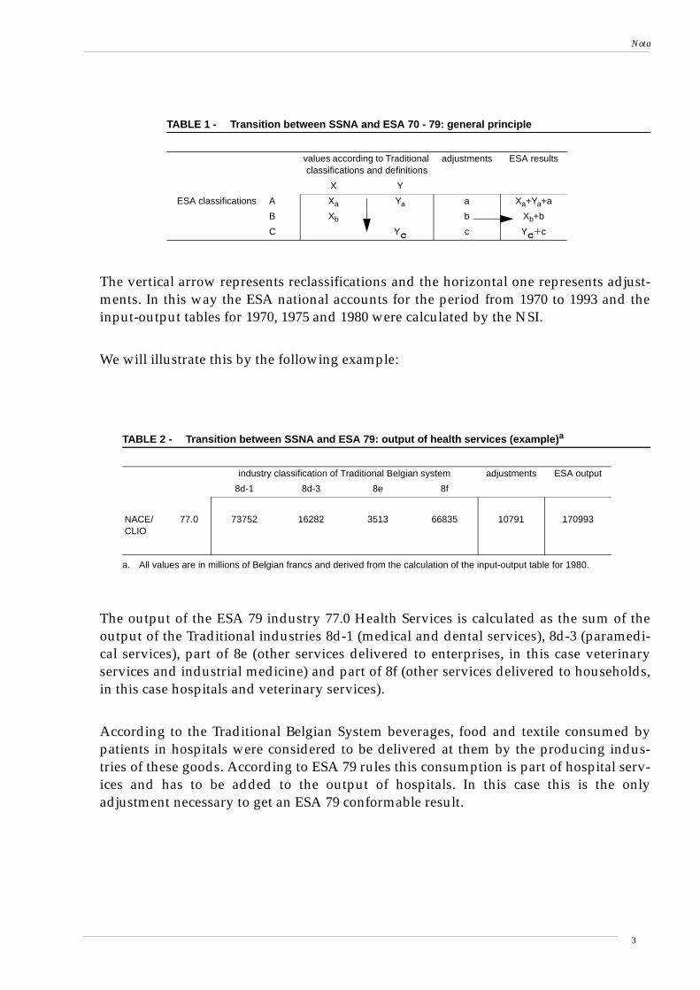
The vertical arrow represents reclassifications and the horizontal one represents adjust-ments. In this way the ESA national accounts for the period from 1970 to 1993 and theinput-output tables for 1970, 1975 and 1980 were calculated by the NSI.

We will illustrate this by the following example:

The output of the ESA 79 industry 77.0 Health Services is calculated as the sum of theoutput of the Traditional industries 8d-1 (medical and dental services), 8d-3 (paramedi-cal services), part of 8e (other services delivered to enterprises, in this case veterinaryservices and industrial medicine) and part of 8f (other services delivered to households,in this case hospitals and veterinary services).

According to the Traditional Belgian System beverages, food and textile consumed bypatients in hospitals were considered to be delivered at them by the producing indus-tries of these goods. According to ESA 79 rules this consumption is part of hospital serv-ices and has to be added to the output of hospitals. In this case this is the onlyadjustment necessary to get an ESA 79 conformable result.

TABLE 1 - Transition between SSNA and ESA 70 - 79: general principle

values according to Traditionalclassifications and definitions

adjustments ESA results

X Y

ESA classifications A Xa Ya a Xa+Ya+a

B Xb b Xb+b

C Yc c Yc+c

TABLE 2 - Transition between SSNA and ESA 79: output of health services (example)a

a. All values are in millions of Belgian francs and derived from the calculation of the input-output table for 1980.

industry classification of Traditional Belgian system adjustments ESA output

8d-1 8d-3 8e 8f

NACE/CLIO

77.0 73752 16282 3513 66835 10791 170993

3

Nota

2. The organizational reform

In a revision of the Public Statistics Act, Belgium’s statistical apparatus was significantlyreformed in 19949. Three organisations are now involved in the compilation of nationalaccounts:

• the NSI is still responsible for the collection of statistical data

• the compilation of national accounts, including supply and use tables but excludinginput-output tables has come within the authority of the central bank (National Bank ofBelgium - NBB)

• the Federal Planning Bureau has been given the mission of compiling the input-outputtables

The Federal Planning Bureau (FPB) is a public agency under the authority of the PrimeMinister and the Minister of Economic Affairs. The legal status of the FPB gives it anautonomy and intellectual independence within the Belgian public sector. The FPB’sactivities are primarily focused on macro-economic forecasting, analysing and assessingpolicies in the economic, social and environmental fields. Its main activity is carrying outeconomic studies for the Belgian government, parliament and institutions for delibera-tions between the social partners (trade unions, employers and self-employed people).

The word “planning” in the name is only a remnant of the responsibility during the1970s for the compilation of five-year economic plans, indicative for the private sectorbut compulsory for the public sector. The last of these plans covered the 1975-1980period.

In order to coordinate the activities of these three institutions a new institute was cre-ated: the Institute for National Accounts (INA). Its activity merely involves supervisionof the actual compilation work done by the three institutions. The creation of this struc-ture was intended to meet the requirements following the introduction of the ESA 95.During the first years of its existence the INA also published ESA 79 based nationalaccounts. The national accounts for 1994-1997 and the input-output tables for 1985 and199010 were still compiled according to the ESA 79 accounting rules and used the “old”methodology of the NSI.

9. Loi du 4 juillet 1962 relative à la statistique publique, modifiée par les lois du 1er août 1985 et 21 décembre 1994.10. The input-output table for 1985 was published in 1998 and-, the one for 1990 in 1999. The last input-output table compiled by the NSI,

for 1980 was published in 1988. This was really a catch-up on operation.

4

Nota

3. The new ESA 95 national accounts

a. Calculation of GDP

Only the general principles and salient features of the production account (output, interme-diate consumption, value added) and the generation of income account (components ofvalue added) will be explained here11. It is not our intention to describe the complete sys-tem developed by the central bank, but only the part of it that is relevant to the input-out-put system. It has been decided to make maximum use of administrative data,supplemented if necessary by specific surveys. The reasons for doing this are:

• to keep the administrative burden on enterprises as low as possible. Using existing datasources means that less additional interrogation of enterprises is needed

• administrative data cover individual enterprises and are nearly exhaustive. This makesdetailed compilations possible and reduces the need for extrapolations

One outstanding administrative source is the so called “Central Balance Sheet Office” of theNBB. In Belgium almost all non-financial corporations have to submit their annualaccounts to this institution. Corporations have to draw up their annual account accordingto a legally determined accounting system. The summaries that have to be submitted to theCentral Balance Sheet Office are based on this legal framework. Two different reportingschemes are distinguished according to the size of the enterprise:

• large corporations have to submit detailed accounts

• smaller corporations12 only have to submit summary accounts

The data in the summary accounts of small enterprises are supplemented:

• by the use of other administrative sources: Value Added Tax (VAT) data (sales, pur-chases), social security data (wages)

• according to the fixed system of proportions based on the data from large corporationswithin the same sector of activity

11. Final demand (the expenditure approach of GDP) will be described as part of the use table.12. The difference between large and small corporations is determined by law.

5

Nota

The administrative data are converted into ESA aggregates13.

The items in the accounts cannot simply be added up in order to calculate the ESA aggre-gates. A series of corrections has to be made in order to arrive at values consistent with ESA95 concepts and definitions. The necessary information is obtained through surveys.Instead of conducting a complete new survey an existing one has been extended, namelythe Structural Business Statistics (also a product of European regulation)14.

About 40,000 enterprises are surveyed by the NSI.

• large corporations (detailed accounts) receive a detailed questionnaire

• small corporations do receive a simplified questionnaire

Items are added to the questionnaires to obtain the necessary information for the conver-sion to ESA 95 aggregates.

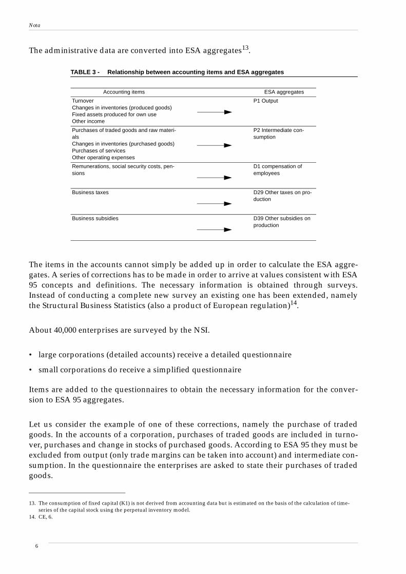
Let us consider the example of one of these corrections, namely the purchase of tradedgoods. In the accounts of a corporation, purchases of traded goods are included in turno-ver, purchases and change in stocks of purchased goods. According to ESA 95 they must beexcluded from output (only trade margins can be taken into account) and intermediate con-sumption. In the questionnaire the enterprises are asked to state their purchases of tradedgoods.

TABLE 3 - Relationship between accounting items and ESA aggregates

Accounting items ESA aggregates

TurnoverChanges in inventories (produced goods)Fixed assets produced for own useOther income

P1 Output

Purchases of traded goods and raw materi-alsChanges in inventories (purchased goods)Purchases of servicesOther operating expenses

P2 Intermediate con-sumption

Remunerations, social security costs, pen-sions

D1 compensation ofemployees

Business taxes D29 Other taxes on pro-duction

Business subsidies D39 Other subsidies onproduction

13. The consumption of fixed capital (K1) is not derived from accounting data but is estimated on the basis of the calculation of time-series of the capital stock using the perpetual inventory model.

14. CE, 6.

6

Nota

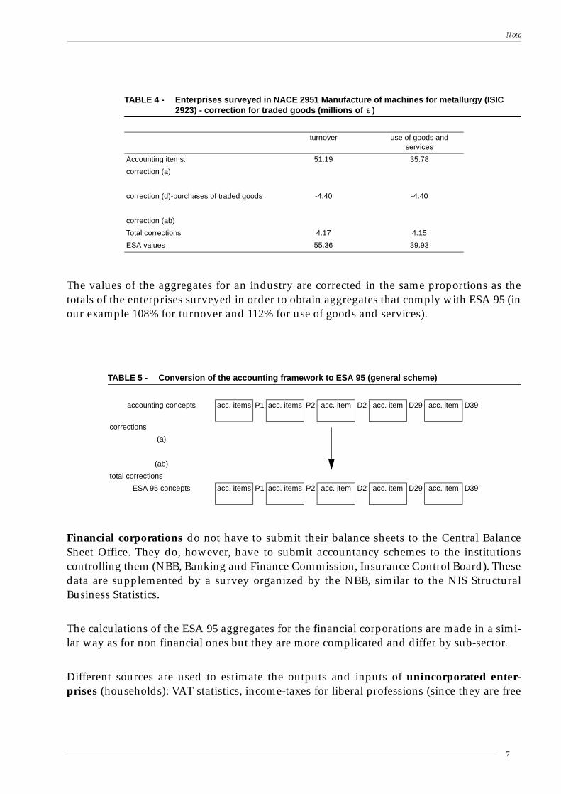
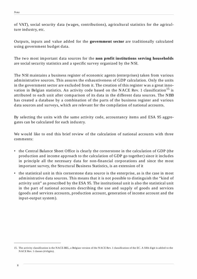
The values of the aggregates for an industry are corrected in the same proportions as thetotals of the enterprises surveyed in order to obtain aggregates that comply with ESA 95 (inour example 108% for turnover and 112% for use of goods and services).

Financial corporations do not have to submit their balance sheets to the Central BalanceSheet Office. They do, however, have to submit accountancy schemes to the institutionscontrolling them (NBB, Banking and Finance Commission, Insurance Control Board). Thesedata are supplemented by a survey organized by the NBB, similar to the NIS StructuralBusiness Statistics.

The calculations of the ESA 95 aggregates for the financial corporations are made in a simi-lar way as for non financial ones but they are more complicated and differ by sub-sector.

Different sources are used to estimate the outputs and inputs of unincorporated enter-prises (households): VAT statistics, income-taxes for liberal professions (since they are free

TABLE 4 - Enterprises surveyed in NACE 2951 Manufacture of machines for metallurgy (ISIC2923) - correction for traded goods (millions of )

turnover use of goods andservices

Accounting items: 51.19 35.78

correction (a)

correction (d)-purchases of traded goods -4.40 -4.40

correction (ab)

Total corrections 4.17 4.15

ESA values 55.36 39.93

TABLE 5 - Conversion of the accounting framework to ESA 95 (general scheme)

accounting concepts acc. items P1 acc. items P2 acc. item D2 acc. item D29 acc. item D39

corrections

(a)

(ab)

total corrections

ESA 95 concepts acc. items P1 acc. items P2 acc. item D2 acc. item D29 acc. item D39

ε

7

Nota

of VAT), social security data (wages, contributions), agricultural statistics for the agricul-ture industry, etc.

Outputs, inputs and value added for the government sector are traditionally calculatedusing government budget data.

The two most important data sources for the non profit institutions serving householdsare social security statistics and a specific survey organized by the NSI.

The NSI maintains a business register of economic agents (enterprises) taken from variousadministrative sources. This assures the exhaustiveness of GDP calculation. Only the unitsin the government sector are excluded from it. The creation of this register was a great inno-vation in Belgian statistics. An activity code based on the NACE Rev. 1 classification15 isattributed to each unit after comparison of its data in the different data sources. The NBBhas created a database by a combination of the parts of the business register and variousdata sources and surveys, which are relevant for the compilation of national accounts.

By selecting the units with the same activity code, accountancy items and ESA 95 aggre-gates can be calculated for each industry.

We would like to end this brief review of the calculation of national accounts with threecomments:

• the Central Balance Sheet Office is clearly the cornerstone in the calculation of GDP (theproduction and income approach to the calculation of GDP go together) since it includesin principle all the necessary data for non-financial corporations and since the mostimportant survey, the Structural Business Statistics, is an extension of it

• the statistical unit in this cornerstone data source is the enterprise, as is the case in mostadministrative data sources. This means that it is not possible to distinguish the “kind ofactivity unit” as prescribed by the ESA 95. The institutional unit is also the statistical unitin the part of national accounts describing the use and supply of goods and services(goods and services accounts, production account, generation of income account and theinput-output system).

15. The activity classification is the NACE-BEL, a Belgian version of the NACE Rev. 1 classification of the EC. A fifth digit is added to theNACE Rev. 1 classes (4 digits).

8

Nota

• the difference between GDP calculated according to the old methodology (ESA 79) andthe new one (ESA 95) is very limited. The overall difference is caused not only by theconceptual differences between the two accounting frameworks but also by the intro-duction of new data sources and compilation methodologies. For 1995 (the first baseyear of the ESA 95 national accounts) the ESA 95 GDP is about 0.8% higher than the ESA79 one. The conceptual innovations in ESA 95 do generally have an upward effect onGDP16. Many of them enhance final demand and value added. The NBB has calculatedthe total effect of these innovations separately. They amounted to 1.9% of GDP. Thismeans that the effect of the introduction of new data sources and compilation techniquesis negative: about -1.1%. The old methodology thus overestimated GDP within theframework of ESA 79.

b. Use and Supply tables compiled by the NBB

The supply and use tables are compiled according to the framework set out in chapter 9 ofthe ESA 95 manual. This is the first time such a system has been created in Belgium. In thepast input-output tables were compiled without the intermediate stage of supply and usetables. The ESA 70 and 79 did not prescribe the compilation of supply and use tables, butonly input-output tables. In the past this was one of the great differences between the ESAand SNA 68 accounting systems.

323 products and 122 industries are distinguished. The products are mainly a regrouping ofthe CPA classes (4 digits) and, the industries of the NACE Rev. 1 groups (3 digits).

The information used in compilation of the output and intermediate consumption sub-matrices in use and supply tables is mainly gathered through the Structural Business Statis-tics. About 8000 of the 40000 enterprises surveyed also received annexes in which they

16. The conceptual differences between the SNA 93 (basis of the ESA 95 - UN, 27.) and the SNA 68 (basis of ESA 70 and ESA 79 - UN, 23.)are explained in annex I of the SNA 93.

TABLE 6 - The number of goods and services in the use and supply tables in the framework ofthe P6 and A6 classifications

P6 (products) A6 (industries)

A + B Agriculture 12 3

C + D + E Industry 195 60

F Construction 19 5

G + H + I Distribution and communication 35 (incl. 2 margins) 16

J + K Business services 30 (incl. FISIMa service)

a. financial intermediation services indirectly measured

16 (incl. the FISIM nomi-nal industry)

L to P Other services 32 22

Total 323 122

9

Nota

were asked to split certain items in their accounts (turnover17, intermediate purchases) byproduct. Finally the declarations of 1698 enterprises were considered suitable for the analy-sis of turnover and, 1572 for the analysis of intermediate purchases. These data were usedto split up total output (P1) and total intermediate consumption of the industries (P2) intothe 323 products.

It is not possible to describe here the data sources and compilation of the other parts of thesupply and use tables and the arbitration process in detail. We simply would like to men-tion that:

• the components of value added by industry are already calculated during the compila-tion of the production account and the primary distribution of income account and arehardly changed at all during the arbitration process

• the compilation of the column of final consumption expenditure by households islargely based on a budget survey of households organised by the NSI

• more or less the same data sources are used for calculation of final consumption expend-iture by non-profit institutions serving households and by government as those used inthe calculation of the production of these services

• gross fixed capital formation by product is estimated by means of the commodity flowmethod (total supply - other uses) in such a way that total investment by industry isrespected. This latter is calculated using balance sheet data (supplemented by the Struc-tural Business Statistics results) and VAT statistics.

• administrative data concerning changes in inventories are found in the balance sheetdata. Information detailed by type of goods is requested in the annexes of the StructuralBusiness Statistics (quantities only)

• total imports and exports of goods and services are derived from the balance of pay-ments. Imports and export of goods are subdivided on the basis of foreign trade statis-tics18 while imports and exports of services are subdivided on the basis of balance ofpayment data.

C. The compilation of the input-output table

1. Starting point: supply and use tables

These are described in the previous section. We would like to stress a few salient features ofthe supply and use tables received from the NBB.

17. Only the total output of manufacturing goods is asked. This can be further analysed by consulting the industrial PRODCOM statistic(Council Regulation (EEC) n° 3924/91 of 19 December 1991 on the establishment of a Community survey of industrial production).

18. In Belgium these are collected by the NBB.

10

Nota

Although the working format of the supply and use tables includes 323 products and 122industries, it is only minimal as a starting point for the compilation of the input-outputtable:

• individual elements in the supply table are valued at basis/CIF prices, in the use table atpurchaser prices, excl. non-deductible VAT. No use table at basis/CIF prices has beencalculated by the NBB. There are no trade and transport margins, product taxes and sub-sidies tables with the exception of a table for non-deductible VAT. This has already beenremoved from the individual elements of intermediate and final demand and added upin a single row as part of value added.

• the use table is not split up in a table for domestic output and for imports

• final consumption expenditure by households is modelled on a territorial basis as in theESA 79 input-output tables and not on a national basis as prescribed by the ESA 95. Thismeans that:

- expenditure by non-resident tourists in the Belgian economic territory is part ofhousehold final consumption expenditure and not of exports

- expenditure by Belgian tourists abroad is not taken into consideration

• only one product is distinguished for trade margins and one for transport margins. Thisis not enough. A product can be a characteristic product of only one industry. In a squareinput-output system each industry needs just one characteristic product, in a rectangularone each industry needs at least one. The report format demanded by EUROSTAT isbased on the A60 and P60 version of the NACE Rev. 1 and CPA classifications and hasthree industries that produce trade margins as a characteristic product:

- NACE 50 Sale, maintenance and repair of motor vehicles and motorcycles; retail saleof automotive fuel

- NACE 51 Wholesale trade and commission trade services, except of motor vehiclesand motorcycles

- NACE 52 Retail trade services, except motor vehicles and motorcycles; repair servicesof personal and household goods

This means that at least three different types of trade margins should be distinguished.In the working format the trade in motor vehicles (NACE 501 to 504) and retail sales ofautomotive fuel (NACE 505) are two different industries. If this format is to maintainedwhen compiling the input-output table at least 4 different trade margins should be dis-tinguished.The distinction of two transport margins is a required minimum since the EUROSTATreport- format contains 2 industries of which transport margins are a characteristic prod-uct19:

- NACE 60 Land transport and transport via pipelines

19. Due to the geography of Belgium it is assumed that air transport services (NACE 62) do not produce transport margins.

11

Nota

- NACE 61 Water transport services

Forwarding and transport insurance margins are ignored although they are explicitlyprescribed by the EUROSTAT input-output manual20. The working format contains 3industries of which transport margins are a characteristic product:

- Transport via railways (NACE 601)

- Freight transport by roads and transport via pipelines (NACE 6024 + 603, ISIC 6023 +60321)

- Inland water transport (NACE 612)22

This means that at least three types of transport margins should be considered if onewishes to maintain the working format when compiling the input-output table.

• Because the statistical unit is the enterprise it might be supposed that the supply table isvery heterogeneous: the industries should have substantial secondary activities. This isindeed the case. The ratio of total secondary output to total output is used as a criterion:the ratio of total off-diagonal elements to total elements in the make matrix (the outputsub-matrix of the supply table), after aggregation to a square matrix. This seems to be aself-evident measure although it is also criticized23. The value of this ratio was 15%. Atthis stage the two groups of industries of which trade and transport margins are charac-teristic products each had to be incorporated into a single industry when aggregating toa square make matrix. 15% is thus the level of heterogeneity of a 117x11724 make matrixand not of a 122x122 one.

2. Desaggregation of industries for analytical purposes

The A60 version of the NACE Rev. 1 does not distinguish between:

• the manufacture of cokes, refined petroleum and nuclear fuel (all in NACE 23)

• the manufacture of different basic metals (all in NACE 27)

• the supply of electricity and natural gas (both in NACE 40)

• renting of real estate and intermediate services regarding real estate (both in NACE 70)

The working format of the supply and use tables includes the industries 23, 40 and 70 assuch and does not fully distinguish between production of ferrous and non-ferrous metals.

20. EUROSTAT, 12.21. ISIC and NACE codes are nearly always equal. We only give the corresponding ISIC code when this is not the case.22. For identical reasons the same assumption is made for sea and coastal water transport (NACE 611) as for air transport.23. Konijn, 15. It includes the output of industries that only have secondary production (cfr. below) but does not take so-called by-prod-

ucts or joint product into account since they remain classified with the main product to which they are technologically fixed.24. Or rather of a 116 x 116 matrix since the FISIM industry does not have a production.

12

Nota

The only distinction made is between the production of ECSC25 and non-ECSC ferrousmetals.

The FPB has decided to desaggregate these industries in order to make these distinctions.This was not originally intended for statistical reasons (to facilitate the calculation of theinput-output table: essentially the derivation of non-negative technical coefficients26) but toextend the use of the input-output table as an instrument of economic analysis:

• it is certainly useful to distinguish between electricity and gas supply. These are com-pletely different activities.

• the ESA 79 input-output tables used a version of the NACE/CLIO classification in whichall those distinctions did exist. In order to make comparisons with these it is better tohave a version of the ESA 95 input-output table in which this distinction is maintained

• it is better to keep the supply and use of the different energy products separated in orderto have a better link with energy statistics

The industries are desaggregated in the same way as the original compilation whereverpossible: the same data sources and methodology are used. For the separation of energyproduction one additional statistic is used: the energy statistics from the Energy depart-ment of the Ministry of Economic affairs. These reflect the use and supply of energy prod-ucts (at a more detailed product level but a less detailed industry level than the supply anduse tables) in quantities and serve as a basis for the energy balances of EUROSTAT.

3. Valuation matrices

a. Product taxes and subsidies matrices

The matrix of non-deductible VAT was already calculated by the NBB. The matrices ofimport duties and levies on agricultural products are simultaneously calculated with theuse table for imports of goods.

The compilation of the product taxes and subsidies table is barely discussed at all in eco-nomic literature. In fact only the EUROSTAT input-output manual gives a few hints in rela-tion to its compilation:

• the allocation of product taxes by product (compilation of the column(s) of product taxesand subsidies in the supply tables) should be done by consulting the revenue data of the

25. European Coal and Steel Community. This treaty has expired on July 23 2002. Of course ISIC does not distinguish ECSC and non-ECSC activities.

26. The complete separation of the manufacture of ferrous and non-ferrous metals has rather complicated this derivation. The desaggre-gations of the energy industries did unintentionally lead to the detection of important errors in the original supply and use tables (cfr.below).

13

Nota

fiscal authorities. In fact we found that it is necessary to study fiscal legislation in orderto do this correctly.

• The distribution of the total amount of each product tax or subsidy over the elements ofthe use table should be done by consulting fiscal legislation in order to:

- find appropriate tax/subsidy rates

- discover which parts of final and/or intermediate use are exempted or taxed/subsi-dized at lower rates

We found that it is not possible to translate fiscal legislation entirely into the framework ofthe input-output system. Fiscal legislation is far too complex:

• the official tax rates are mostly not expressed in terms of the purchaser prices at whichthe use table is valued. Tax rates are usually expressed in terms of quantities or other val-ues than the purchaser prices of the goods and services in the use table.

• if there are different tax rates for a given tax, each tax rate should be applied to one prod-uct only. In order to achieve this an impossible number of products would have to beentered in the input-output system.

• in order to take into account all exemptions or lower tax- rates for specific uses theindustries would have to be broken up into an impossible number of activities

For all these reasons we have resorted to a rather simple method for the distribution ofproduct taxes and subsidies. A more sophisticated method has been developed for exciseduties.

The simple method consists of a adapted proportional distribution of the total amount ofeach product tax/subsidy over the row(s) of the products to which they apply, taking fiscallegislation into account as far as possible:

• certain elements are excluded from the proportional distribution if they correspond touses that are not taxed/subsidized

• only a fraction of an element is taken into account if it is a use that is taxed at a favoura-ble tax rate

Of course not all the details of fiscal legislation could be taken into account.

Most product taxes are consumer taxes. In this case the following rules are applicable mostof the time:

• final consumption expenditure by households is fully taxed

• exports are not taxed at all

14

Nota

• for certain intermediate uses there are exemptions or favourable tax rates

For product taxes that only cover domestic production and all subsidies on products27 theuse table for domestic output is used as a distribution key.

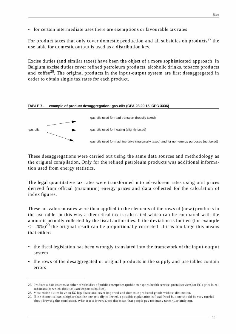
Excise duties (and similar taxes) have been the object of a more sophisticated approach. InBelgium excise duties cover refined petroleum products, alcoholic drinks, tobacco productsand coffee28. The original products in the input-output system are first desaggregated inorder to obtain single tax rates for each product.

These desaggregations were carried out using the same data sources and methodology asthe original compilation. Only for the refined petroleum products was additional informa-tion used from energy statistics.

The legal quantitative tax rates were transformed into ad-valorem rates using unit pricesderived from official (maximum) energy prices and data collected for the calculation ofindex figures.

These ad-valorem rates were then applied to the elements of the rows of (new) products inthe use table. In this way a theoretical tax is calculated which can be compared with theamounts actually collected by the fiscal authorities. If the deviation is limited (for example<= 20%)29 the original result can be proportionally corrected. If it is too large this meansthat either:

• the fiscal legislation has been wrongly translated into the framework of the input-outputsystem

• the rows of the desaggregated or original products in the supply and use tables containerrors

27. Product subsidies consist either of subsidies of public enterprises (public transport, health service, postal services) or EC agriculturalsubsidies (of which about 2/3 are export subsidies).

28. Most excise duties have an EC legal base and cover imported and domestic produced goods without distinction.

TABLE 7 - example of product desaggregation: gas-oils (CPA 23.20.15, CPC 3336)

gas-oils used for road transport (heavily taxed)

gas-oils gas-oils used for heating (slightly taxed)

gas-oils used for machine-drive (marginally taxed) and for non-energy purposes (not taxed)

29. If the theoretical tax is higher than the one actually collected, a possible explanation is fiscal fraud but one should be very carefulabout drawing this conclusion. What if it is lower? Does this mean that people pay too many taxes? Certainly not.

15

Nota

These additional checks are not possible using the simple method.

b. The trade margins table

This table (which gives the part of the trade margin in the use of each good30) has been cal-culated simultaneously with the table for the use of imported goods. The compilation ofthese two matrices is the object of a separate paper presented at this conference31. Only thegeneral principles will be mentioned here.

The supply table gives only the total trade margins for each good and the total trade pro-duced by each industry, without further distinction. The main data source which made itpossible to combine the calculation of the trade margins table and the use table forimported goods is the foreign trade statistics which give imports and exports of goods byimporting and exporting industries.

Finally, five different trade margins were introduced into the input-output system becauseit was considered useful to separate wholesale of fuels from the rest of the wholesale indus-try. This means that the supply table had to be extended. Few data exist about the type oftrade margins produced by each industry. The trade margins realized by non-trade indus-tries are largely estimated on the basis of data for imports and exports of traded goods,derived from foreign trade statistics. It is supposed that trade in industrial and most serviceindustries is wholesale while trade in some specific service industries is retail. The divisionof total trade margins realized by each trade service industry into one principal and foursecondary ones is largely done by economic reasoning due to the lack of data32.

The reason why the trade margins table has been calculated simultaneously with the usetable for imported goods is that a great deal of information about trade activities can bederived directly or with only a few manipulations from foreign trade statistics:

• transactions without the interference of trade (and thus without the realization of trademargins):

- direct imports by the industries using intermediate and investment goods

- direct exports by the producer of the goods33

• trade margins realized by industry

• imports by retail sale industries: the bulk of these goods are disposed of with only retailsale margins realised

• imports of goods that can be identified as consumer goods at the level of the interna-tional trade classification

30. Trade margins represent about 13% of the total value of total use of goods.31. Van den Cruyce, 29.32. The Structural Business Statistics give only detailed information about sales not about trade margins.33. These are an important part of total transactions in goods in a small open economy like Belgium.

16

Nota

Finally wholesale and retail trade margin ratios are calculated for each good. It is supposedthat retail trade margins are only realized on final consumption expenditure by house-holds. On the other parts of final demand and intermediate use only wholesale trade mar-gins are realized. Finally a fixed ratio between wholesale and retail trade margins rates wassupposed, differing by good in the input-output system where possible.

c. The transport margins table

This has been calculated in a simple way, because of two reasons:

• the very narrow definition of transport margins in the ESA 95. These have to be invoicedseparately to the purchaser of the goods.

• the lack of information

Only one total transport margin was considered in the original supply table. This row(transport margins produced by each industry) could be desaggregated easily because:

• the transport industries have no secondary transport activity in relation to transportmargins. They only produce their characteristic margin.

• the other industries are only involved in road transport

The transport margins column (total transport margins by good) was desaggregated intocolumns for each type of transport margin on the basis of the data used to calculate thetransport margins by producing industry. The NBB constructed a table of transport mar-gins by transported good as realized by the producing industries34.

The total for each transport margin by good was then proportionally distributed over eachrow of the use table. For some goods there was no transport margin attributed to final con-sumption expenditures by households. These were goods for which it was assumed thatthe households themselves carry out the transport (for example non-durable consumptiongoods).

4. Use tables for imports and for domestic input

Many countries seem to resort to a simple proportional distribution of imports over eachrow of the use table. This means that it is accepted that the ratio of import to total supplyis valid for each element. The consequences of such a simple assumption should be con-sidered. Input-output tables are mainly used for economic analysis. Essential in input-output applications are the so-called multiplier effects. These are solely caused by theinput-output table for domestic output, which is derived from the use table for domestic

34. As mentioned before, each industry produces only one type of transport margin. In this way the industries are homogeneous.

17

Nota

output. An excessively simplistic calculation of the latter makes the use of input-outputtables less reliable as an instrument for economic analysis.

At least for the use table of imported goods it was possible to allocate a considerable partof imports more or less exactly to its uses35. By exploring the data from the foreign tradestatistics, the following parts of imports could be attributed immediately or after only afew manipulations:

• the so called “special” transactions (for example goods that are temporarily imported fornon-significant processing to order or repair36). These are allocated to exports.

• merchanting: imports of these goods were also allocated to exports37

• direct imports by non-trade industries. A large part of these can be allocated to interme-diate use and investments.

• imports of consumption goods by trade industries. These are largely destined for finalconsumption expenditures by households.

Finally, almost 70% of the total value of imported goods could be allocated directly to thevarious intermediate and final uses. The rest is distributed proportionally over theremaining elements of the use table (excluding direct exports).

As regards imports of services, the poor quality of the balance of payments data made asimilar approach impossible. The services imported are distributed proportionally overthe rows of the use table. As in the case of the product tax and subsidies matrices, how-ever, this is an adapted proportional distribution. This time certain elements of the rowsare excluded from the distribution on the basis of economic rules. There are, for example,no exports of imported services, with the exception of imported transport margins.

5. The calculation of symmetric input-output tables

a. Starting point and aims

After the introduction of the valuation matrices described above, the margins, producttaxes and subsidies are redistributed, resulting in a valuation of all elements of the use tableat basic prices.

Only a product x product input-output table is calculated, not a industry x industry one.This is the case because EUROSTAT only requires the calculation of the first one and mostinput-output applications need the product x product variant38.

35. Since this is the subject of a separate paper, only the general principles will be mentioned here.36. These were left in the original supply and use tables, contradictory to ESA 95 principles.37. They were also not removed from imports and exports, also in contradiction to ESA 95 principles.38. In fact, we are not aware of input-output applications where a industry x industry version is required.

18

Nota

We began with a completely mechanical compilation of the input-output table derivedfrom the supply and use table as received from the NBB, even before the valuation matriceswere compiled. This “prototype” was gradually improved by the introduction of the valua-tion matrices, correction of data and desaggregation of industries.

Essential in the compilation of product x product tables is the choice of the mathematicaltransformation method of inputs used for secondary output. We have preferred producttechnology to industry technology, for two reasons.

The SNA 93 judges the industry technology principle as highly implausible. Almon39 givesa good example and considers the recommendation and use of the industry technologyassumption “little short of scandalous”. Examples of the absurdity of the industry technol-ogy assumption are endless. Industrial industries do have considerable secondary produc-tion of wholesale activities and conversely wholesale enterprises produce large amounts ofgoods as a secondary activity. Applying the industry technology principle here implies theattribution of industrial inputs (raw materials, semi-manufactured articles) to wholesaleactivities, which of course does not make sense. Industry technology only seems to beacceptable for a small minority of secondary products technologically related to primaryoutput (by-products, joint products).

But there is more than this. Kop Jansen and ten Raa40 have put forward four necessaryrequirements which an input-output matrix should fulfil in order to be usable as an instru-ment of economic analysis as put forward by the founding- father of input-output analysis,W. Leontiev41. These four criteria have become “institutionalised” by their introduction inthe SNA 93 and the accompanying UN handbook of input-output tables42. Only the com-modity technology assumption fulfils these four requirements. An input-output table com-piled on the basis of industry technology is therefore unusable as an instrument ofeconomic analysis while this is exactly the raison d’être of input-output tables since theyare bypassed as a statistical equilibrium tool by the system of supply and use tables.

b. the first (base) estimation

This is an input-output table derived from the supply and use tables received from the NBBwith no desaggregations of products and industries except the minimal necessary desag-gregation of distribution margins, which was done arbitrarily. All the valuation matriceswere calculated almost completely proportional, following the sequence described in theinput-output manual. Commodity technology was uniformly used except in two caseswhere it was mathematically impossible:

39. Almon, 2.40. Kop Jansen, ten Raa, 17.41. Material balance (supply = use), financial balance (output = costs), scale invariance (the technical coefficients should be invariant to

the level of production) and price invariance (the constant price estimate of the input-output table should be invariant to price fluctu-ations).

42. UN, 28.

19

Nota

• metal ores are only produced as a secondary activity and the NACE Division 13 Miningof metal ores must be distinguished in the report format by EUROSTAT. Applying thecommodity technology is impossible here because the square product-mix matrix is notinvertible: it has a non-zero row and a corresponding zero column.

• The industry NACE 37 Recycling has no characteristic production, only secondary prod-ucts! Recycled goods are reclassified as the goods normally produced because the use ofrecycled and original goods could not be distinguished in the use table. In this case thesquare product-mix matrix is also not invertible because it has a zero row and a corre-sponding non-zero column.

In these two cases industry technology was applied. This was mathematically added to the(almost) general use of commodity technology by means of the hybrid technology model asformulated in the SNA 68.

The basic matrices in the conversion toward the input-output table are:

the make matrix:

(1)

This is the output part of the supply table. Compared to the system described in table 5,three trade and two transport margins are added, according to a Belgian tradition theFISIM industry is aggregated with the financial intermediation services (NACE 65), onenominal industry is added for energy producing materials (NACE 10-12) which are onlyimported and one industry for mining of metal ores (NACE 13). A homogeneous branchwill be created for this last one although there is no industry (enterprises) for this activity inthe use table43.

The absorption matrix44 :

(2)

This is the intermediate part of the use table: we maintained the rows of total product taxes,subsidies and imported transport margins in order to keep total intermediate use of eachindustry valued at purchaser prices, incl. non deductible VAT.

The square make matrix:

43. We take product x industry as the dimensions of the make matrix, unlike the SNA 68 where it was industry x product.44. We use the terminology of the former input-output manual of the UN, supplementary to the SNA 68: UN, 24.

V

328x123( )

U

333x128( )

20

Nota

(3)

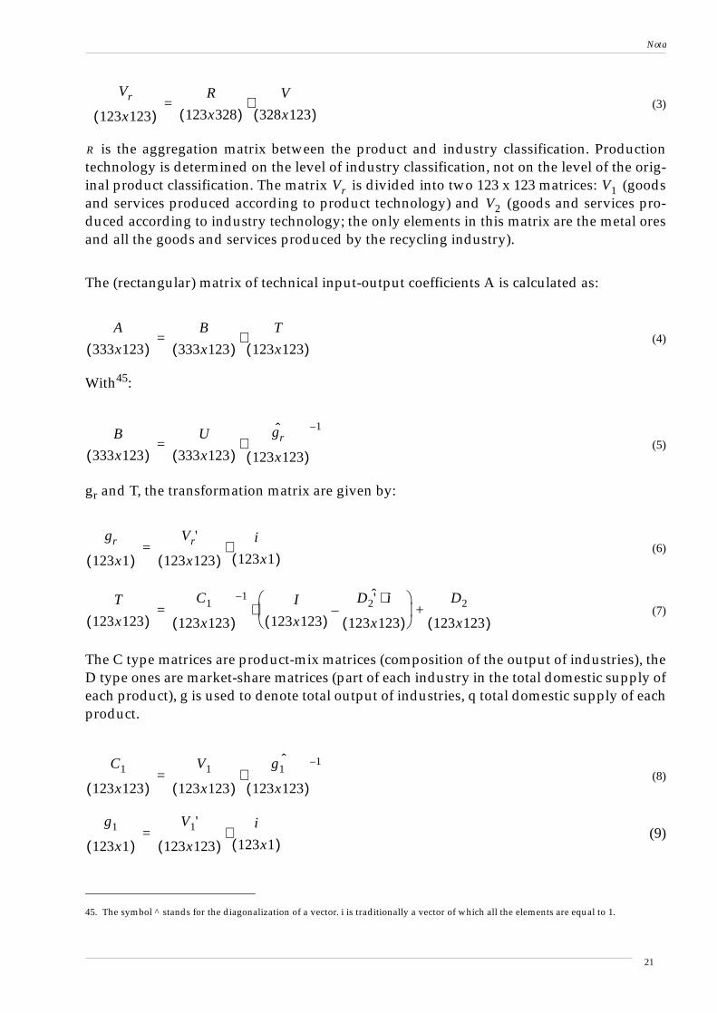
is the aggregation matrix between the product and industry classification. Productiontechnology is determined on the level of industry classification, not on the level of the orig-inal product classification. The matrix is divided into two 123 x 123 matrices: (goodsand services produced according to product technology) and (goods and services pro-duced according to industry technology; the only elements in this matrix are the metal oresand all the goods and services produced by the recycling industry).

The (rectangular) matrix of technical input-output coefficients A is calculated as:

(4)

With45:

(5)

gr and T, the transformation matrix are given by:

(6)

(7)

The C type matrices are product-mix matrices (composition of the output of industries), theD type ones are market-share matrices (part of each industry in the total domestic supply ofeach product), g is used to denote total output of industries, q total domestic supply of eachproduct.

(8)

(9)

45. The symbol ^ stands for the diagonalization of a vector. i is traditionally a vector of which all the elements are equal to 1.

Vr

123x123( )R

123x328( )V

328x123( )⋅=

R

Vr V1V2

A

333x123( )B

333x123( )T

123x123( )⋅=

B

333x123( )U

333x123( )gr

123x123( )

ˆ 1–

⋅=

gr

123x1( )

Vr'

123x123( )i

123x1( )⋅=

T

123x123( )C1

123x123( )

1– I

123x123( )D2' i⋅

123x123( )

ˆ–

⋅D2

123x123( )+=

C1

123x123( )

V1

123x123( )

g1

123x123( )

1–ˆ⋅=

g1

123x1( )

V1'

123x123( )i

123x1( )⋅=

21

Nota

(10)

(11)

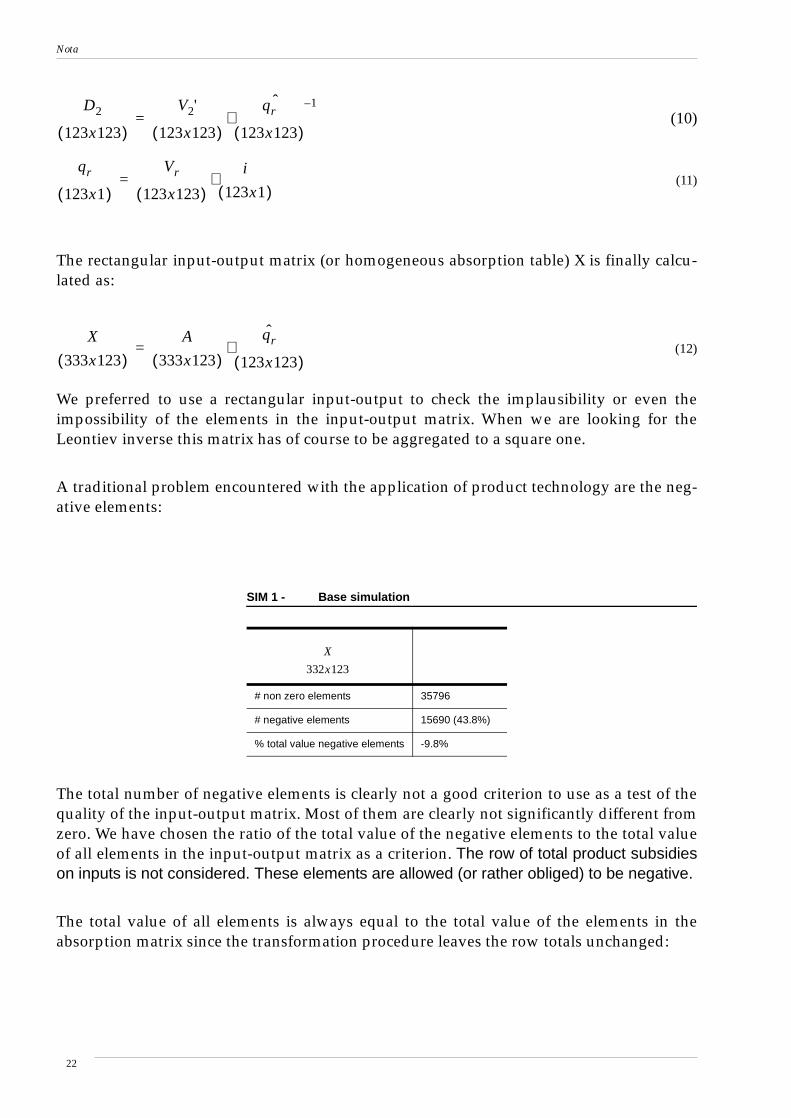
The rectangular input-output matrix (or homogeneous absorption table) X is finally calcu-lated as:

(12)

We preferred to use a rectangular input-output to check the implausibility or even theimpossibility of the elements in the input-output matrix. When we are looking for theLeontiev inverse this matrix has of course to be aggregated to a square one.

A traditional problem encountered with the application of product technology are the neg-ative elements:

The total number of negative elements is clearly not a good criterion to use as a test of thequality of the input-output matrix. Most of them are clearly not significantly different fromzero. We have chosen the ratio of the total value of the negative elements to the total valueof all elements in the input-output matrix as a criterion. The row of total product subsidieson inputs is not considered. These elements are allowed (or rather obliged) to be negative.

The total value of all elements is always equal to the total value of the elements in theabsorption matrix since the transformation procedure leaves the row totals unchanged:

SIM 1 - Base simulation

# non zero elements 35796

# negative elements 15690 (43.8%)

% total value negative elements -9.8%

D2

123x123( )

V2'

123x123( )

qr

123x123( )

1–ˆ⋅=

qr

123x1( )

Vr

123x123( )i

123x1( )⋅=

X

333x123( )A

333x123( )qr

123x123( )

ˆ⋅=

X

332x123

22

Nota

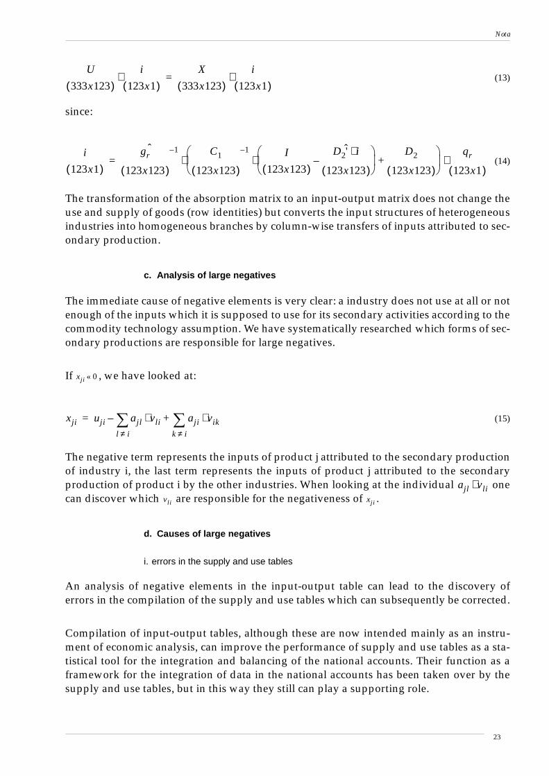
(13)

since:

(14)

The transformation of the absorption matrix to an input-output matrix does not change theuse and supply of goods (row identities) but converts the input structures of heterogeneousindustries into homogeneous branches by column-wise transfers of inputs attributed to sec-ondary production.

c. Analysis of large negatives

The immediate cause of negative elements is very clear: a industry does not use at all or notenough of the inputs which it is supposed to use for its secondary activities according to thecommodity technology assumption. We have systematically researched which forms of sec-ondary productions are responsible for large negatives.

If , we have looked at:

(15)

The negative term represents the inputs of product j attributed to the secondary productionof industry i, the last term represents the inputs of product j attributed to the secondaryproduction of product i by the other industries. When looking at the individual onecan discover which are responsible for the negativeness of .

d. Causes of large negatives

i. errors in the supply and use tables

An analysis of negative elements in the input-output table can lead to the discovery oferrors in the compilation of the supply and use tables which can subsequently be corrected.

Compilation of input-output tables, although these are now intended mainly as an instru-ment of economic analysis, can improve the performance of supply and use tables as a sta-tistical tool for the integration and balancing of the national accounts. Their function as aframework for the integration of data in the national accounts has been taken over by thesupply and use tables, but in this way they still can play a supporting role.

U

333x123( )i

123x1( )⋅

X

333x123( )i

123x1( )⋅=

i

123x1( )gr

123x123( )

1–ˆ C1

123x123( )

1– I

123x123( )D2' i⋅

123x123( )

ˆ–

⋅D2

123x123( )+

qr

123x1( )⋅ ⋅=

xji 0«

xji uji ajl vli⋅l i≠∑ aji vik⋅

k i≠∑+–=

ajl vli⋅vli xji

23

Nota

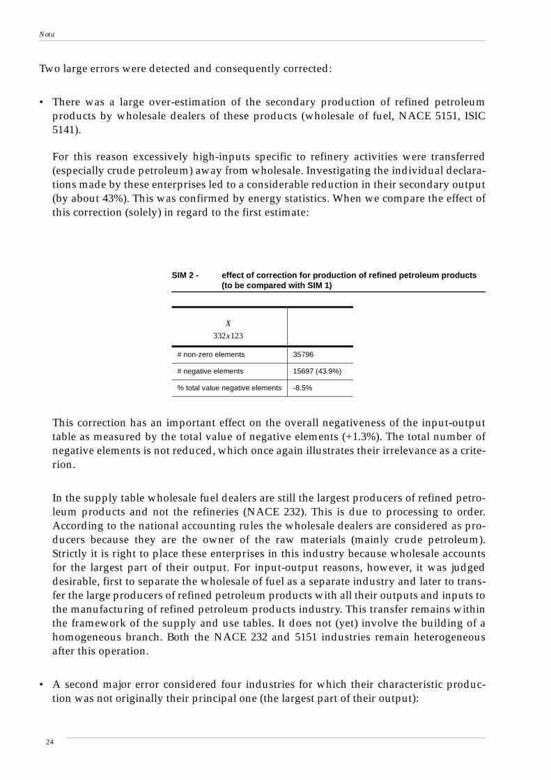
Two large errors were detected and consequently corrected:

• There was a large over-estimation of the secondary production of refined petroleumproducts by wholesale dealers of these products (wholesale of fuel, NACE 5151, ISIC5141).

For this reason excessively high-inputs specific to refinery activities were transferred(especially crude petroleum) away from wholesale. Investigating the individual declara-tions made by these enterprises led to a considerable reduction in their secondary output(by about 43%). This was confirmed by energy statistics. When we compare the effect ofthis correction (solely) in regard to the first estimate:

This correction has an important effect on the overall negativeness of the input-outputtable as measured by the total value of negative elements (+1.3%). The total number ofnegative elements is not reduced, which once again illustrates their irrelevance as a crite-rion.

In the supply table wholesale fuel dealers are still the largest producers of refined petro-leum products and not the refineries (NACE 232). This is due to processing to order.According to the national accounting rules the wholesale dealers are considered as pro-ducers because they are the owner of the raw materials (mainly crude petroleum).Strictly it is right to place these enterprises in this industry because wholesale accountsfor the largest part of their output. For input-output reasons, however, it was judgeddesirable, first to separate the wholesale of fuel as a separate industry and later to trans-fer the large producers of refined petroleum products with all their outputs and inputs tothe manufacturing of refined petroleum products industry. This transfer remains withinthe framework of the supply and use tables. It does not (yet) involve the building of ahomogeneous branch. Both the NACE 232 and 5151 industries remain heterogeneousafter this operation.

• A second major error considered four industries for which their characteristic produc-tion was not originally their principal one (the largest part of their output):

SIM 2 - effect of correction for production of refined petroleum products(to be compared with SIM 1)

# non-zero elements 35796

# negative elements 15697 (43.9%)

% total value negative elements -8.5%

X

332x123

24

Nota

- Manufacture of pesticides and other agro-chemical producers (NACE 242, ISIC 2421)

- Treatment and coating of metals, general chemical engineering (NACE 285, ISIC 2892)

- Site preparation (NACE 451)

- Retail sale of automotive fuels (NACE 505)

When looking at the basic data the reason for this aberration was found: some enter-prises used to divide up total outputs and inputs of these industries were wrongly classi-fied in the business register.

Simply recalculating the columns of the last three industries in the supply and use tables,not taking these enterprises into account, was a solution for the last three industries. Butthe first one was in fact dominated by one very large and wrongly classified enterprise.Like the wholesale dealers with a large production of refined petroleum products its out-puts and inputs were transferred to the industry where it really belonged (Manufactureof basic chemicals, NACE 241).

Unfortunately, it is impossible to get an idea of the importance of this correction as noversion exists which takes only this modification into account.

ii.Heterogeneity of the industry classification

Many authors do indicate this as a possible cause of negatives when applying the producttechnology model46. The UN and EUROSTAT manuals also emphasize this.

When calculating the input structures of products (homogeneous branches) these areaggregated to the level of the industry classification. At this level the principal productionof an industry is an aggregation of different original products for which the productionprocesses (inputs) may differ in reality. The input structure of a homogeneous branch islargely determined by the input structure of the primary producer. This means that theinput structure of a homogeneous branch is more or less a weighted average of the inputstructures of the original products made by the primary producer. Another industry canproduce, as a secondary activity, only some of these original products or in a different com-position from the primary producer. But this is not taken into account in the transformationmatrix of the commodity technology model ( ). It is assumed here that secondary pro-ducers have the same composition as the main one. If this is not the case (large) negativescan be created in the input-output table.

Let us take as an example: the production of railway locomotives and rolling stock (CPA352, CPC 495 and (partly) 8868) by railway companies (NACE 601). This is output for ownfinal use (gross fixed capital formation). The principal producer of these goods is a combi-

46. Gigantes 13, Konijn 15 and 16 , Rainer 19 and 20, Stone, 21.

11–

25

Nota

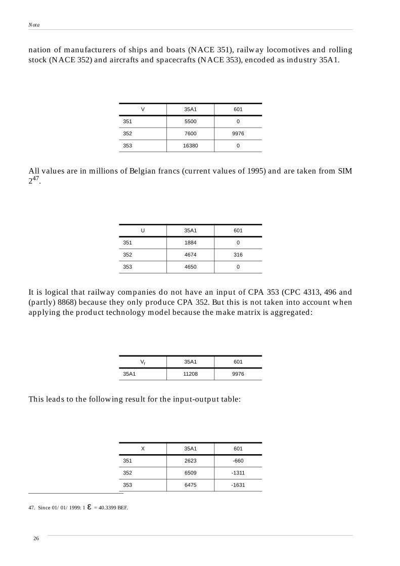
nation of manufacturers of ships and boats (NACE 351), railway locomotives and rollingstock (NACE 352) and aircrafts and spacecrafts (NACE 353), encoded as industry 35A1.

All values are in millions of Belgian francs (current values of 1995) and are taken from SIM247.

It is logical that railway companies do not have an input of CPA 353 (CPC 4313, 496 and(partly) 8868) because they only produce CPA 352. But this is not taken into account whenapplying the product technology model because the make matrix is aggregated:

This leads to the following result for the input-output table:

V 35A1 601

351 5500 0

352 7600 9976

353 16380 0

47. Since 01/01/1999: 1 = 40.3399 BEF.

U 35A1 601

351 1884 0

352 4674 316

353 4650 0

Vr 35A1 601

35A1 11208 9976

X 35A1 601

351 2623 -660

352 6509 -1311

353 6475 -1631

ε

26

Nota

The large negative input of aircraft and spacecraft in railway transport is easily explained:railway companies do not produce aircraft or spacecraft and they therefore do not have anyintermediary use of aircraft and spacecraft (parts). They are, however, supposed to do soaccording the product technology model because it uses the aggregated version of themake matrix.

One obvious solution to this problem is a desaggregation of the industry 35A1 into threeseparate industries, NACE 351, NACE 352 and NACE 353. In this case only inputs properto the principal activity of NACE 352 will be transferred away from NACE 601 and not air-craft and spacecraft (parts).

This was not sufficient to eliminate all large negatives in CPA 601. The railway companyhas a very low input of CPA 352 compared to the industries in which NACE 352 is the prin-cipal activity. This has caused a large negative input of CPA 352 in CPA 601 in the input-output table, which probably means that transport material produced by railway compa-nies still differs from the one produced by NACE 352 as a principal activity. Finally outputfor own final use of locomotives and rolling stock and construction work by railway com-panies were considered as separate activities and products. This is an example of “analyti-cal” desaggregation since it is not a regrouping of enterprises (statistical units in the input-output system) but manual partitioning of an enterprise into not (fully) observable parts.

e. Correction of negatives

Various types of improvements were made. Let us consider these by category

i. Correction of the supply and use tables

Errors discovered while calculating the input-output table were reported to the makers ofthe supply and use tables. This feedback should be considered to be a normal procedure inthe compilation of national accounts. In reality, input-output tables can not be consideredas a mere mathematical derivation of supply and use tables. All the errors reported wererectified except when enterprises had to be moved from one industry to another. Thiswould imply an alteration in the business register, which is only done periodically. Theseshifts were carried out by the FPB for the compilation of the input-output table only. Thismeans that already at this stage of compilation there is a difference between what Rainerand Richter call descriptive use and supply tables (part of national accounts) and analyticalones (modified ones from which the input-output table is derived)48.

Let us consider the base version after feedback from the NBB and the following modifica-tions:

• transfers between industries (switching of enterprises)

48. Rainer, Richter 20.

27

Nota

• product desaggregations that will facilitate the calculation of the product tax and subsi-dies matrices at a later stage

• industry desaggregations for analytical reasons

• the desaggregation of the wholesale fuels industry (which means the introduction of anadditional margin)

The product tax, subsidies and distribution margins matrices are still calculated propor-tionally.

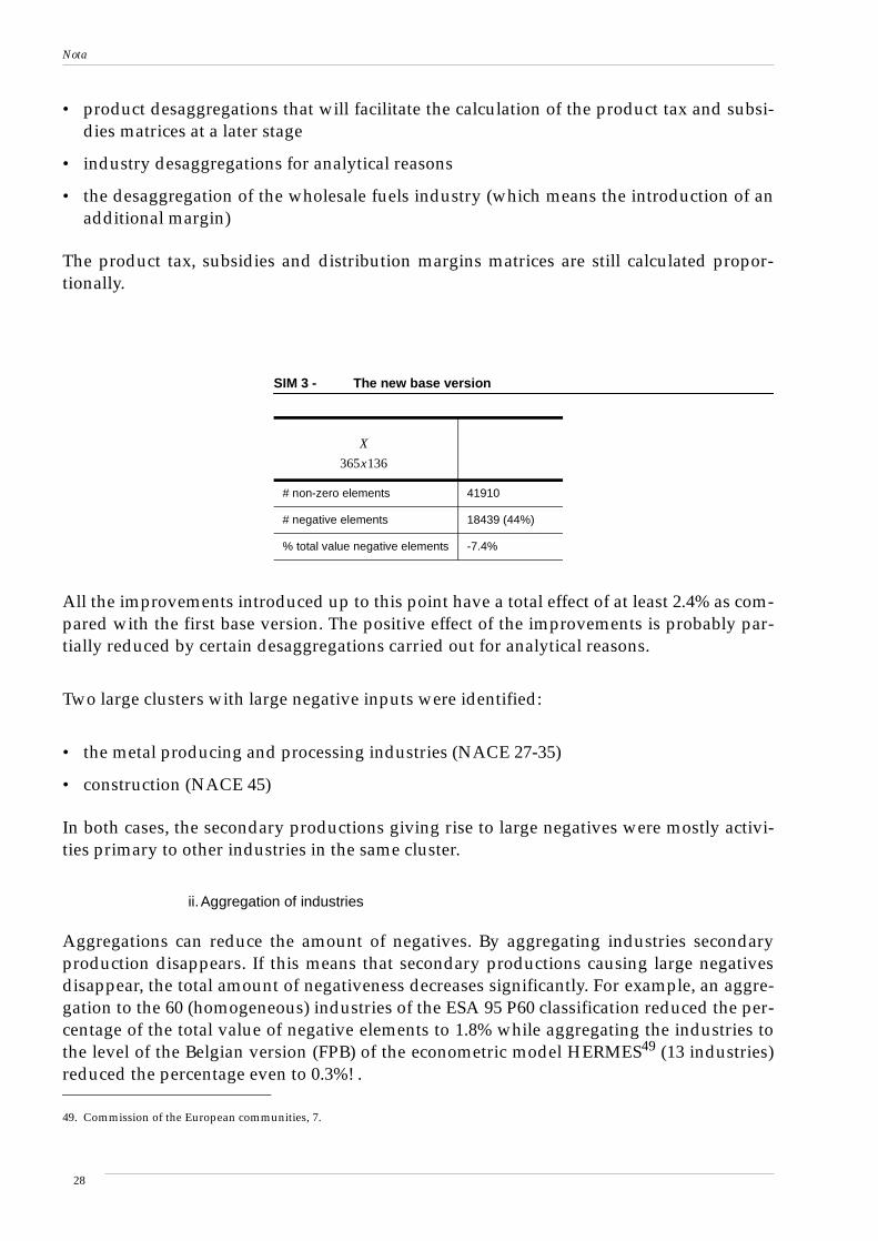
All the improvements introduced up to this point have a total effect of at least 2.4% as com-pared with the first base version. The positive effect of the improvements is probably par-tially reduced by certain desaggregations carried out for analytical reasons.

Two large clusters with large negative inputs were identified:

• the metal producing and processing industries (NACE 27-35)

• construction (NACE 45)

In both cases, the secondary productions giving rise to large negatives were mostly activi-ties primary to other industries in the same cluster.

ii.Aggregation of industries

Aggregations can reduce the amount of negatives. By aggregating industries secondaryproduction disappears. If this means that secondary productions causing large negativesdisappear, the total amount of negativeness decreases significantly. For example, an aggre-gation to the 60 (homogeneous) industries of the ESA 95 P60 classification reduced the per-centage of the total value of negative elements to 1.8% while aggregating the industries tothe level of the Belgian version (FPB) of the econometric model HERMES49 (13 industries)reduced the percentage even to 0.3%! .

SIM 3 - The new base version

# non-zero elements 41910

# negative elements 18439 (44%)

% total value negative elements -7.4%

X

365x136

49. Commission of the European communities, 7.

28

Nota

This can be done very easily but the input-output team is not favourable to this solution,for two reasons:

• the report format required by EUROSTAT uses NACE Rev. 1 divisions (2 digits). Thismeans that only industries belonging to the same NACE Rev. 1 division can be aggre-gated.

• even when this is the case, we were not very favourable to this easy solution. In order totake as many future applications into account as possible, it is better not to aggregateindustries. Aggregating all construction activities into one industry would resolve thenegatives-problem in the second cluster almost completely50. But when it comes to stud-ying the effect of government measures to stimulate the construction of dwellings orlarge public works, for example, it is recommended to keep the original number ofindustries intact.

Up until now (July 2002) no aggregations have been carried out or planned.

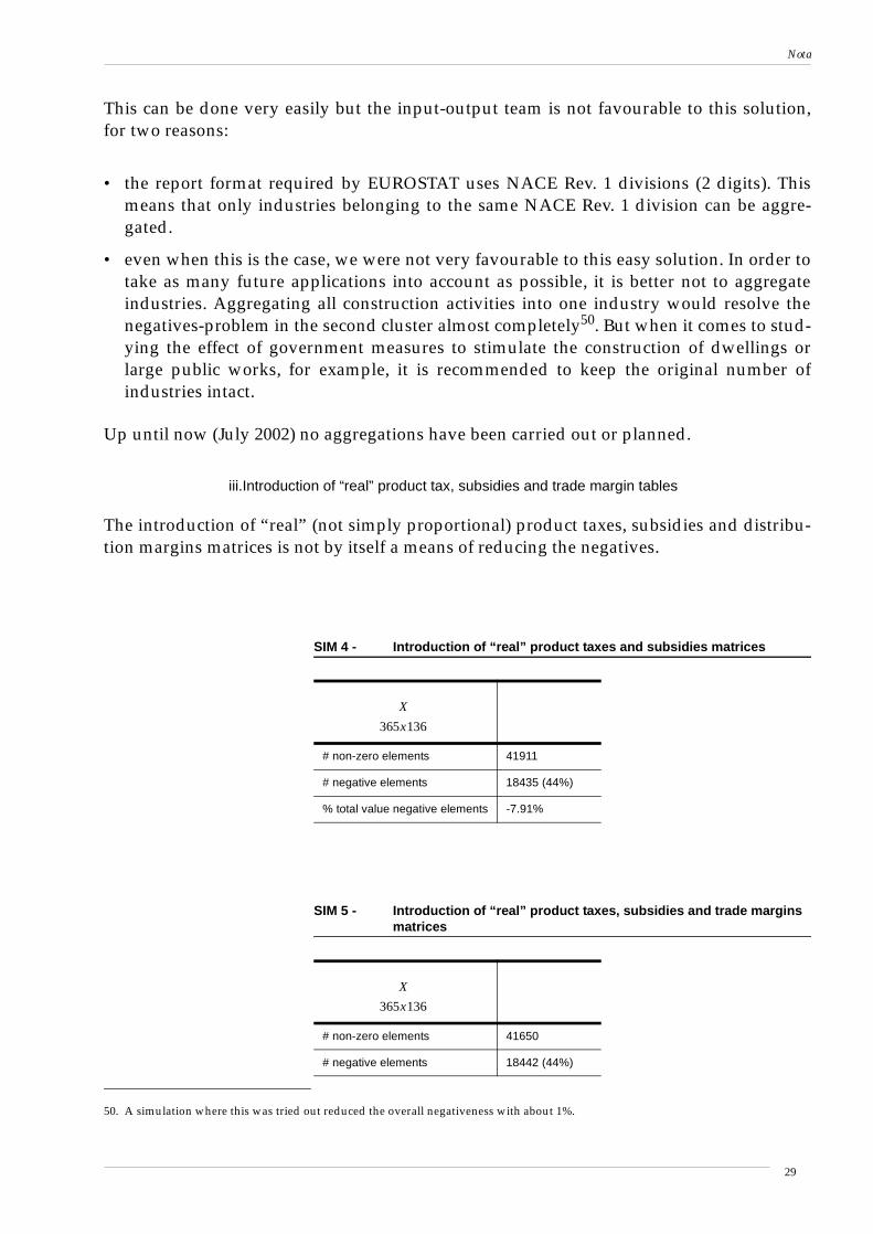
iii.Introduction of “real” product tax, subsidies and trade margin tables

The introduction of “real” (not simply proportional) product taxes, subsidies and distribu-tion margins matrices is not by itself a means of reducing the negatives.

50. A simulation where this was tried out reduced the overall negativeness with about 1%.

SIM 4 - Introduction of “real” product taxes and subsidies matrices

# non-zero elements 41911

# negative elements 18435 (44%)

% total value negative elements -7.91%

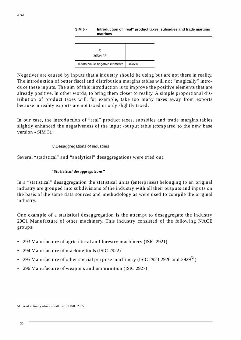
SIM 5 - Introduction of “real” product taxes, subsidies and trade marginsmatrices

# non-zero elements 41650

# negative elements 18442 (44%)

X

365x136

X

365x136

29

Nota

Negatives are caused by inputs that a industry should be using but are not there in reality.The introduction of better fiscal and distribution margins tables will not “magically” intro-duce these inputs. The aim of this introduction is to improve the positive elements that arealready positive. In other words, to bring them closer to reality. A simple proportional dis-tribution of product taxes will, for example, take too many taxes away from exportsbecause in reality exports are not taxed or only slightly taxed.

In our case, the introduction of “real” product taxes, subsidies and trade margins tablesslightly enhanced the negativeness of the input -output table (compared to the new baseversion - SIM 3).

iv.Desaggregations of industries

Several “statistical” and “analytical” desaggregations were tried out.

“Statistical desaggregations”

In a “statistical” desaggregation the statistical units (enterprises) belonging to an originalindustry are grouped into subdivisions of the industry with all their outputs and inputs onthe basis of the same data sources and methodology as were used to compile the originalindustry.

One example of a statistical desaggregation is the attempt to desaggregate the industry29C1 Manufacture of other machinery. This industry consisted of the following NACEgroups:

• 293 Manufacture of agricultural and forestry machinery (ISIC 2921)

• 294 Manufacture of machine-tools (ISIC 2922)

• 295 Manufacture of other special purpose machinery (ISIC 2923-2926 and 292951)

• 296 Manufacture of weapons and ammunition (ISIC 2927)

% total value negative elements -8.07%

SIM 5 - Introduction of “real” product taxes, subsidies and trade marginsmatrices

X

365x136

51. And actually also a small part of ISIC 2915.

30

Nota

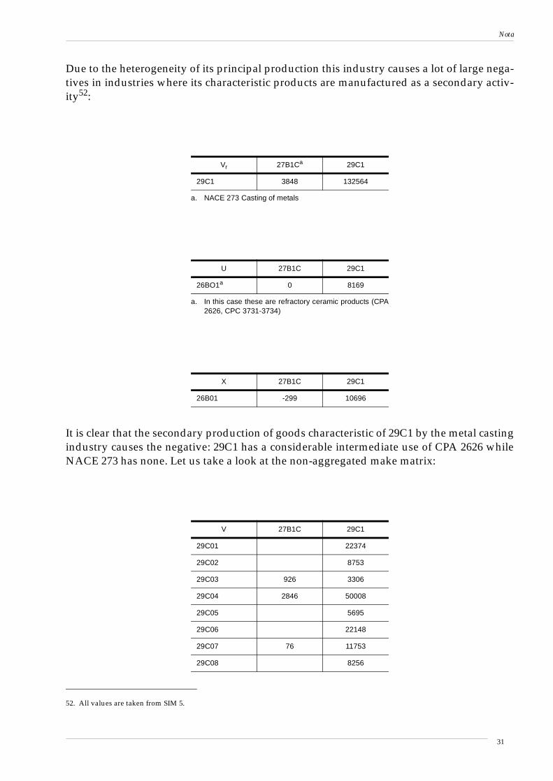
Due to the heterogeneity of its principal production this industry causes a lot of large nega-tives in industries where its characteristic products are manufactured as a secondary activ-ity52:

It is clear that the secondary production of goods characteristic of 29C1 by the metal castingindustry causes the negative: 29C1 has a considerable intermediate use of CPA 2626 whileNACE 273 has none. Let us take a look at the non-aggregated make matrix:

52. All values are taken from SIM 5.

Vr 27B1Ca

a. NACE 273 Casting of metals

29C1

29C1 3848 132564

U 27B1C 29C1

26BO1a

a. In this case these are refractory ceramic products (CPA2626, CPC 3731-3734)

0 8169

X 27B1C 29C1

26B01 -299 10696

V 27B1C 29C1

29C01 22374

29C02 8753

29C03 926 3306

29C04 2846 50008

29C05 5695

29C06 22148

29C07 76 11753

29C08 8256

31

Nota

The meaning of the product codes is as follows:

• 29C01: agricultural and forestry machinery (CPA 293, CPC 441 + part of 8862)

• 29C02: machine- tools (CPA 294, CPC 442 + part of 8862)

• 29C03: machinery for metallurgy (CPA 2951, CPC 443 + part of 8862)

• 29C04: machinery for mining, quarrying and construction (CPA 2952, CPC 444 + part of8862)

• 29C05: machinery for food, beverage and tobacco processing (CPA 2953, CPC 445 + partof 8862)

• 29C06: machinery for textiles, apparel and leather processing (CPA2954, CPC 446 +44814 + part of 8862)

• 29C07: machinery for other special purposes (CPA 2955 + 2956, CPC 449 + part of 8862)

• 29C08: weapons and ammunitions (CPA 296, CPC 447 + part of 8862)

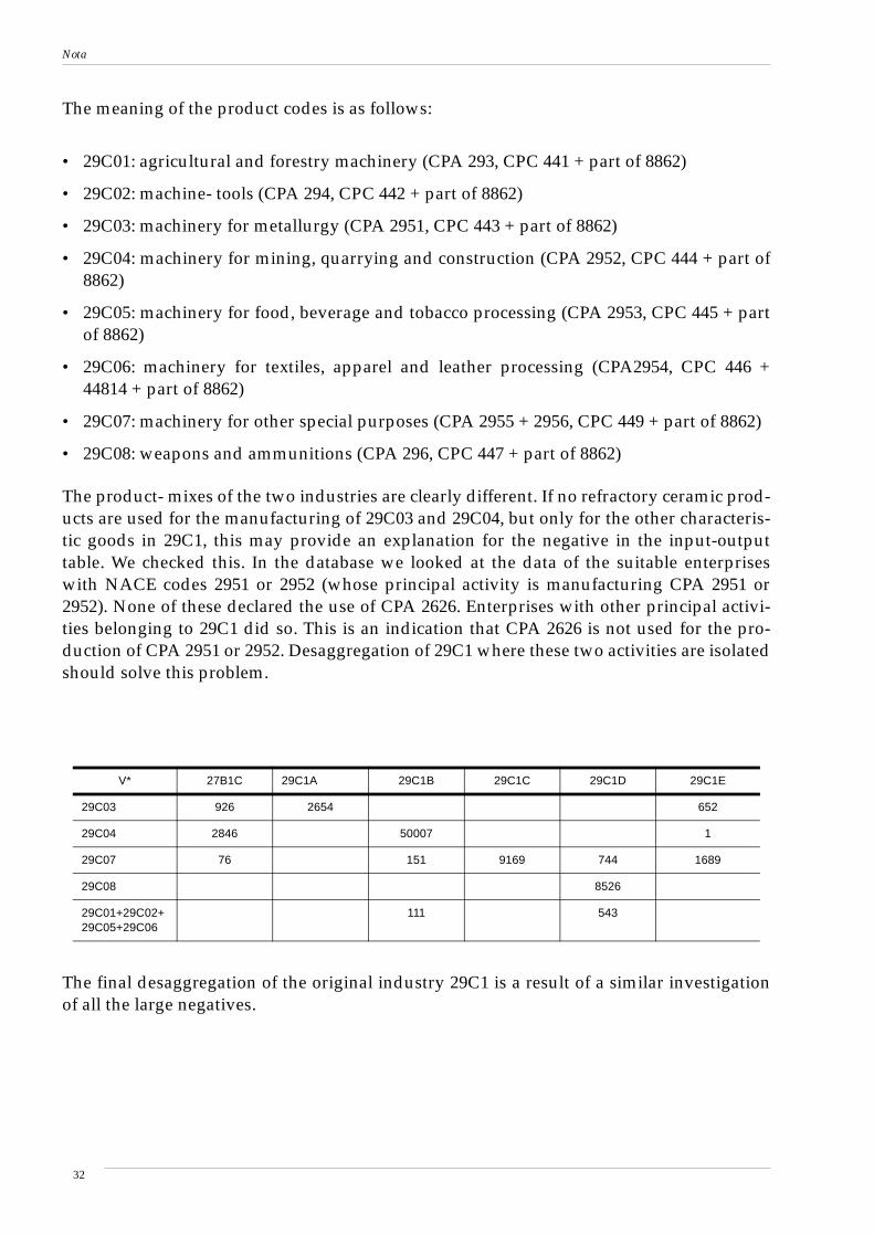
The product- mixes of the two industries are clearly different. If no refractory ceramic prod-ucts are used for the manufacturing of 29C03 and 29C04, but only for the other characteris-tic goods in 29C1, this may provide an explanation for the negative in the input-outputtable. We checked this. In the database we looked at the data of the suitable enterpriseswith NACE codes 2951 or 2952 (whose principal activity is manufacturing CPA 2951 or2952). None of these declared the use of CPA 2626. Enterprises with other principal activi-ties belonging to 29C1 did so. This is an indication that CPA 2626 is not used for the pro-duction of CPA 2951 or 2952. Desaggregation of 29C1 where these two activities are isolatedshould solve this problem.

The final desaggregation of the original industry 29C1 is a result of a similar investigationof all the large negatives.

V* 27B1C 29C1A 29C1B 29C1C 29C1D 29C1E

29C03 926 2654 652

29C04 2846 50007 1

29C07 76 151 9169 744 1689

29C08 8526

29C01+29C02+29C05+29C06

111 543

32

Nota

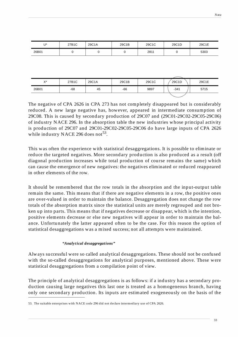
The negative of CPA 2626 in CPA 273 has not completely disappeared but is considerablyreduced. A new large negative has, however, appeared in intermediate consumption of29C08. This is caused by secondary production of 29C07 and (29C01-29C02-29C05-29C06)of industry NACE 296. In the absorption table the new industries whose principal activityis production of 29C07 and 29C01-29C02-29C05-29C06 do have large inputs of CPA 2626while industry NACE 296 does not53.

This was often the experience with statistical desaggregations. It is possible to eliminate orreduce the targeted negatives. More secondary production is also produced as a result (offdiagonal production increases while total production of course remains the same) whichcan cause the emergence of new negatives: the negatives eliminated or reduced reappearedin other elements of the row.

It should be remembered that the row totals in the absorption and the input-output tableremain the same. This means that if there are negative elements in a row, the positive onesare over-valued in order to maintain the balance. Desaggregation does not change the rowtotals of the absorption matrix since the statistical units are merely regrouped and not bro-ken up into parts. This means that if negatives decrease or disappear, which is the intention,positive elements decrease or else new negatives will appear in order to maintain the bal-ance. Unfortunately the latter appeared often to be the case. For this reason the option ofstatistical desaggregations was a mixed success; not all attempts were maintained.

“Analytical desaggregations”

Always successful were so called analytical desaggregations. These should not be confusedwith the so-called desaggregations for analytical purposes, mentioned above. These werestatistical desaggregations from a compilation point of view.

The principle of analytical desaggregations is as follows: if a industry has a secondary pro-duction causing large negatives this last one is treated as a homogeneous branch, havingonly one secondary production. Its inputs are estimated exogeneously on the basis of the

U* 27B1C 29C1A 29C1B 29C1C 29C1D 29C1E

26B01 0 0 0 2811 0 5303

X* 27B1C 29C1A 29C1B 29C1C 29C1D 29C1E

26B01 -68 45 -66 9897 -341 5715

53. The suitable enterprises with NACE code 296 did not declare intermediary use of CPA 2626.

33

Nota

declarations by (almost) homogeneous producers of the product that it generates, foundfrom among the suitable enterprises in the database. When separating this homogeneousbranch from the original industry, care is taken to ensure that no negatives arise in this lastone. In this way, no negatives will ultimately appear in the homogeneous input-outputtable during the transformation procedure. The single (secondary) output of the homoge-neous dummy branches are entered in the V2 matrix to facilitate the calculation. They aresimilar to the recycling industry: they have only secondary production, and dummy princi-pal products (zero row in the use and supply tables). But they are even more simplified:they are already homogeneous in the sense that they only make one type of secondarygood. During the transformation procedure their inputs are simply added to the main partof the homogeneous branch that is mathematically calculated. We call this an “analytical”desaggregation because, as we have said, it is not a regrouping of enterprises (statisticalunits in the input-output system) but a manual partition of an enterprise into not (fully)observable parts.

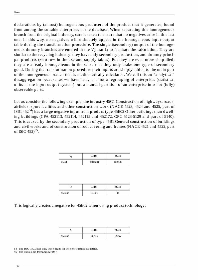
Let us consider the following example: the industry 45C1 Construction of highways, roads,airfields, sport facilities and other construction work (NACE 4523, 4524 and 4525, part ofISIC 45254) has a large negative input from product type 45B02 Other buildings than dwell-ing buildings (CPA 452113, 452114, 452115 and 452172, CPC 5123-5129 and part of 5140).This is caused by the secondary production of type 45B1 General construction of buildingsand civil works and of construction of roof covering and frames (NACE 4521 and 4522, partof ISIC 452)55.

This logically creates a negative for 45B02 when using product technology:

54. The ISIC Rev. 3 has only three digits for the construction industries.55. The values are taken from SIM 5.

Vr 45B1 45C1

45B1 401658 36906

U 45B1 45C1

45B02 24205 0

X 45B1 45C1

45B02 36779 -2967

34

Nota

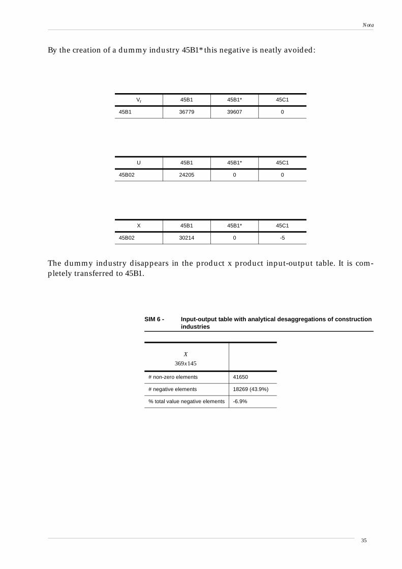
By the creation of a dummy industry 45B1* this negative is neatly avoided:

The dummy industry disappears in the product x product input-output table. It is com-pletely transferred to 45B1.

Vr 45B1 45B1* 45C1

45B1 36779 39607 0

U 45B1 45B1* 45C1

45B02 24205 0 0

X 45B1 45B1* 45C1

45B02 30214 0 -5

SIM 6 - Input-output table with analytical desaggregations of constructionindustries

# non-zero elements 41650

# negative elements 18269 (43.9%)

% total value negative elements -6.9%

X

369x145

35

Nota

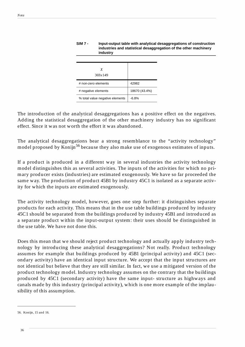
The introduction of the analytical desaggregations has a positive effect on the negatives.Adding the statistical desaggregation of the other machinery industry has no significanteffect. Since it was not worth the effort it was abandoned.

The analytical desaggregations bear a strong resemblance to the “activity technology”model proposed by Konijn56 because they also make use of exogenous estimates of inputs.

If a product is produced in a different way in several industries the activity technologymodel distinguishes this as several activities. The inputs of the activities for which no pri-mary producer exists (industries) are estimated exogenously. We have so far proceeded thesame way. The production of product 45B1 by industry 45C1 is isolated as a separate activ-ity for which the inputs are estimated exogenously.

The activity technology model, however, goes one step further: it distinguishes separateproducts for each activity. This means that in the use table buildings produced by industry45C1 should be separated from the buildings produced by industry 45B1 and introduced asa separate product within the input-output system: their uses should be distinguished inthe use table. We have not done this.

Does this mean that we should reject product technology and actually apply industry tech-nology by introducing these analytical desaggregations? Not really. Product technologyassumes for example that buildings produced by 45B1 (principal activity) and 45C1 (sec-ondary activity) have an identical input structure. We accept that the input structures arenot identical but believe that they are still similar. In fact, we use a mitigated version of theproduct technology model. Industry technology assumes on the contrary that the buildingsproduced by 45C1 (secondary activity) have the same input- structure as highways andcanals made by this industry (principal activity), which is one more example of the implau-sibility of this assumption.

SIM 7 - Input-output table with analytical desaggregations of constructionindustries and statistical desaggregation of the other machineryindustry

# non-zero elements 42982

# negative elements 18670 (43.4%)

% total value negative elements -6.8%

56. Konijn, 15 and 16.

X

369x149

36

Nota

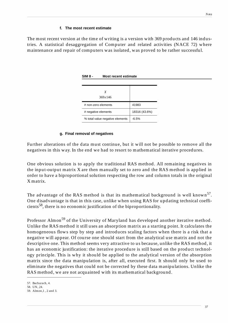
f. The most recent estimate

The most recent version at the time of writing is a version with 369 products and 146 indus-tries. A statistical desaggregation of Computer and related activities (NACE 72) wheremaintenance and repair of computers was isolated, was proved to be rather successful.

g. Final removal of negatives

Further alterations of the data must continue, but it will not be possible to remove all thenegatives in this way. In the end we had to resort to mathematical iterative procedures.

One obvious solution is to apply the traditional RAS method. All remaining negatives inthe input-output matrix X are then manually set to zero and the RAS method is applied inorder to have a biproportional solution respecting the row and column totals in the originalX matrix.

The advantage of the RAS method is that its mathematical background is well known57.One disadvantage is that in this case, unlike when using RAS for updating technical coeffi-cients58, there is no economic justification of the biproportionality.

Professor Almon59 of the University of Maryland has developed another iterative method.Unlike the RAS method it still uses an absorption matrix as a starting point. It calculates thehomogeneous flows step by step and introduces scaling factors when there is a risk that anegative will appear. Of course one should start from the analytical use matrix and not thedescriptive one. This method seems very attractive to us because, unlike the RAS method, ithas an economic justification: the iterative procedure is still based on the product technol-ogy principle. This is why it should be applied to the analytical version of the absorptionmatrix since the data manipulation is, after all, executed first. It should only be used toeliminate the negatives that could not be corrected by these data manipulations. Unlike theRAS method, we are not acquainted with its mathematical background.

SIM 8 - Most recent estimate

# non-zero elements 41983

# negative elements 18316 (43.6%)

% total value negative elements -6.5%

X

369x146

57. Bacharach, 4.58. UN, 24.59. Almon,1 , 2 and 3.

37

Nota

A first test of this method did led to a rather promising result. It was applied to the aggre-gated (square) version of the absorption matrix:

(16)

The Almon procedure was only applied to goods and services produced according to prod-uct technology. The input-output matrix of the products that are part of V2 is still calculatedaccording to industry technology:

(17)

(18)

The inputs for the Almon procedure are the truncated absorption matrix and the matrix ofmarket shares of the goods and services produced according to commodity technology:

(19)

(20)

(21)

The column totals of the complete input-output table:

(22)

are compared with those of the matrix obtained by simple matrix calculation (cfr. above).The differences are altogether limited (a few percentages) except in a few industries whoare characterized by large negatives. These should be handled first in a “statistical” manner(data corrections, desaggregations). The treatment of the value added part should also befurther investigated.

h. Symmetric input-output tables for domestic output and for imports

These are provisionally calculated by applying the transformation matrix T to the absorp-tion tables for domestic output and for imports:

(23)

(24)

Ur R U⋅=

Xrbr Ur g2

ˆ grˆ 1–

C2'⋅ ⋅ ⋅=

C2 V2 g2̂1–

⋅=

Xralm F Ur g1

ˆ grˆ 1–

⋅ ⋅ D1,( )=

D1 V1' q1ˆ 1–

⋅=

q1 V1 i⋅=

Xr Xralm Xr

br+=

Ud T⋅

Um T⋅

38

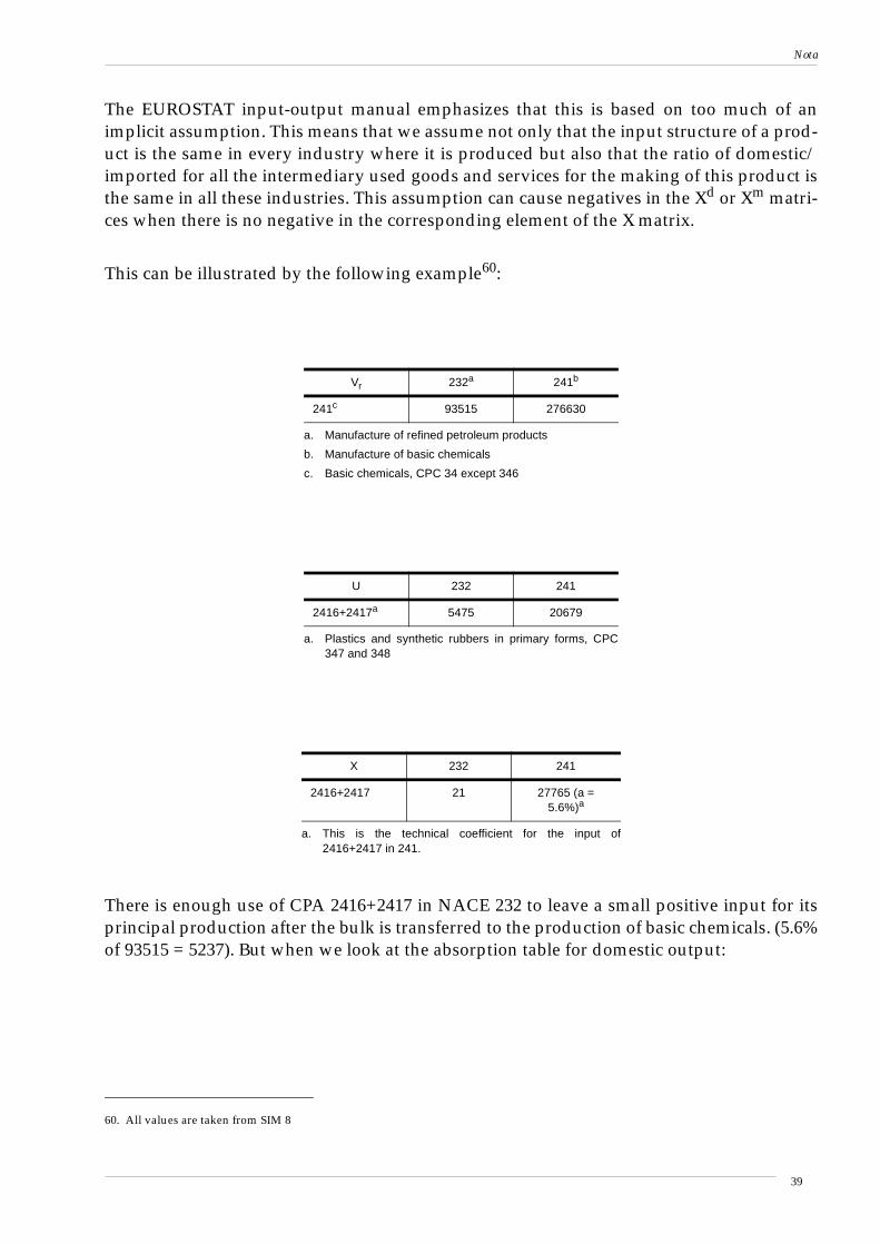
Nota

The EUROSTAT input-output manual emphasizes that this is based on too much of animplicit assumption. This means that we assume not only that the input structure of a prod-uct is the same in every industry where it is produced but also that the ratio of domestic/imported for all the intermediary used goods and services for the making of this product isthe same in all these industries. This assumption can cause negatives in the Xd or Xm matri-ces when there is no negative in the corresponding element of the X matrix.

This can be illustrated by the following example60:

There is enough use of CPA 2416+2417 in NACE 232 to leave a small positive input for itsprincipal production after the bulk is transferred to the production of basic chemicals. (5.6%of 93515 = 5237). But when we look at the absorption table for domestic output:

60. All values are taken from SIM 8

Vr 232a

a. Manufacture of refined petroleum products

241b

b. Manufacture of basic chemicals

241c

c. Basic chemicals, CPC 34 except 346

93515 276630

U 232 241

2416+2417a

a. Plastics and synthetic rubbers in primary forms, CPC347 and 348

5475 20679

X 232 241

2416+2417 21 27765 (a =5.6%)a

a. This is the technical coefficient for the input of2416+2417 in 241.

39

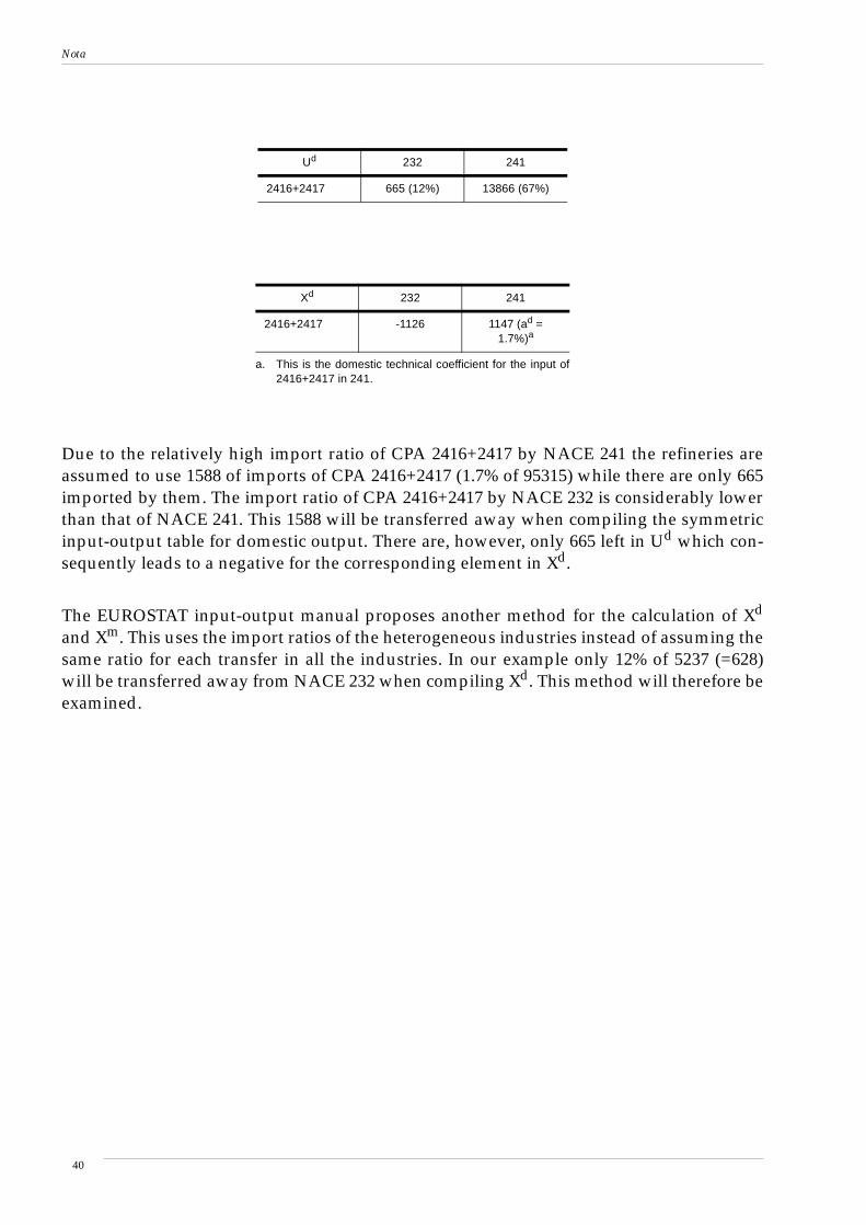
Nota

Due to the relatively high import ratio of CPA 2416+2417 by NACE 241 the refineries areassumed to use 1588 of imports of CPA 2416+2417 (1.7% of 95315) while there are only 665imported by them. The import ratio of CPA 2416+2417 by NACE 232 is considerably lowerthan that of NACE 241. This 1588 will be transferred away when compiling the symmetricinput-output table for domestic output. There are, however, only 665 left in Ud which con-sequently leads to a negative for the corresponding element in Xd.

The EUROSTAT input-output manual proposes another method for the calculation of Xd

and Xm. This uses the import ratios of the heterogeneous industries instead of assuming thesame ratio for each transfer in all the industries. In our example only 12% of 5237 (=628)will be transferred away from NACE 232 when compiling Xd. This method will therefore beexamined.

Ud 232 241

2416+2417 665 (12%) 13866 (67%)

Xd 232 241

2416+2417 -1126 1147 (ad =1.7%)a

a. This is the domestic technical coefficient for the input of2416+2417 in 241.

40

Nota

Bibliography

1. Almon C., Investment in input-output models and the treatment of secondary prod-ucts, Bródy A, Carter A. P. (eds.), Applications of input-output analysis, North-Hol-land, Amsterdam, 1970.

2. Almon C., How to make a product-to-product input-output table, paper presented atthe 12th International conference on input-output techniques, New York, 1998.

3. Almon C., Product-to-product tables via product-technology with no negative flows,Economic Systems Research, volume 12, number 1, March 2000, pp. 27-43.

4. Bacharach M., Biproportional matrices and input-output change, Cambridge Univer-sity Press, Cambridge, 1970.

5. CE, Réglement (CE) n° 2223/96 du Conseil du 25 juin 1996 portant sur le systémeeuropéen de comptes nationaux et régionaux au sein de la Communauté, Journal Offi-ciel des Communautés européennes (L310) du 30 novembre 1996.

6. CE, EURATOM, Réglement (CE, EURATOM) n° 58/97 du Conseil du 20 décembre1996 portant sur des statistiques structurelles des entreprises, Journal Officiel des Com-munautés européennes du 17 janvier 1997.

7. Commision of the European Communities, HERMES: harmonised econometricresearch for modelling economic systems, North-Holand, Amsterdam - London - NewYork - Tokyo, 1993.

8. EUROSTAT, Système Européen de comptes économiques integrés, Luxembourg, 1970.

9. EUROSTAT, European system of integrated economic accounts, Luxembourg, 1979.

10. EUROSTAT, NACE Rev. 1, Council regulation, (EEC) No 3037/90 (O.J. L 293 of24.10.90) as modified by Commission regulation (EEC) No761/93 (O.J.L. 83 of 3.4.93).

11. EUROSTAT, European system of national accounts, ESA 1995, Luxembourg, 1995.

12. EUROSTAT, Eurostat input-output manual, draft, Luxembourg, July 2001.

13. Gigantes T., The representation of technology models in input-output systems, CarterA.P., Brody A. (eds.), Contribution to input-output analysis, North-Holland, Amster-dam, 1970, pg. 270-290.

14. INS, Comptes nationaux 1953-1962, Etudes statistiques et économétriques, numéro 4,1963.

15. Konijn P.J.A, The make and use of commodities by industries, Universiteit Twente,Enschede, 1994.

16. Konijn P.J.A., Steenge A.E., Compilation of input-output data from the nationalaccounts, Economic Systems Research, Vol. 7, No. 1, 1995, pg. 421-435.

17. Kop Jansen P., ten Raa T., The choice of model in the construction of input-output coef-ficients matrices, International Economic Review, vol. 31, No 1, February 1990.

18. OECE, Système normalisé de comptabilité nationale, Paris, 1952.

19. Rainer N., Descriptive versus analytical make-use systems: -some Austrian experi-ences-, Miller R. E., Polenske K., R., Rose A. Z. (eds.), Frontiers of input-output analy-sis, Oxford University Press, New York, Oxford, 1989, pp. 51-64.

20. Rainer N., Richter J., Some aspects of the analytical use of descriptive make andabsorption tables, Economic Systems Research, Vol. 4, No. 2, 1992, pp. 159-172.

41

Nota

21. Stone R., Bates J., Bacharach M. (eds.), A prigram for growth 3, input-output relation-ships 1954-1966, Hapman & Hall, 163.

22. UN, A system of national accounts and supporting tables, Series F, No. 2, New York,1953.

23. UN, A system of national accounts, Series F, No. 2, Rev. 3, New York, 1968.

24. UN, Input-output tables and analysis, Studies in methods, series F., No. 14, rev. 1, NewYork, 1973.

25. UN, International standard industrial classification of all economic activities, thirdrevision, Statistical Papers, Series M, No. 4, Rev. 3, New York, 1990.

26. UN, Provisional central product classification, Statistical Papers, Series M, No. 77, NewYork, 1991.

27. UN, EUROSTAT, IMF, OECD, WB, A system of national accounts 1993, Brussels/Lux-embourg, New York, Paris, Washington, D.C., 1993.

28. UN, Handbook of input-output table compilation and analysis, Studies in methods,series F, No. 74, New York 1999.

29. Van den Cruyce B., An integrated approach to compile the use of imported goods andthe use side trade margins table, paper to be presented at the fourteenth InternationalConference on Input-Output Techniques, Montreal, October 10-15 2002.

42

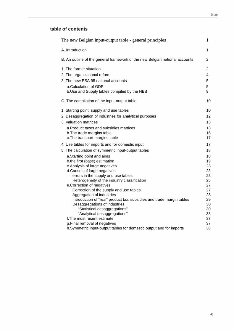
Nota

table of contents

The new Belgian input-output table - general principles 1

A. Introduction 1

B. An outline of the general framework of the new Belgian national accounts 2

1. The former situation 2

2. The organizational reform 4

3. The new ESA 95 national accounts 5

a.Calculation of GDP 5b.Use and Supply tables compiled by the NBB 9

C. The compilation of the input-output table 10

1. Starting point: supply and use tables 10

2. Desaggregation of industries for analytical purposes 12

3. Valuation matrices 13

a.Product taxes and subsidies matrices 13b.The trade margins table 16c.The transport margins table 17

4. Use tables for imports and for domestic input 17

5. The calculation of symmetric input-output tables 18

a.Starting point and aims 18b.the first (base) estimation 19c.Analysis of large negatives 23d.Causes of large negatives 23

errors in the supply and use tables 23Heterogeneity of the industry classification 25

e.Correction of negatives 27Correction of the supply and use tables 27Aggregation of industries 28Introduction of “real” product tax, subsidies and trade margin tables 29Desaggregations of industries 30

“Statistical desaggregations” 30“Analytical desaggregations” 33

f.The most recent estimate 37g.Final removal of negatives 37h.Symmetric input-output tables for domestic output and for imports 38

43