Embed Size (px)
Citation preview
MULTIVARIATE BEHAVIORAL RESEARCH 1
Multivariate Behavioral Research, 37 (1), 1-36Copyright © 2002, Lawrence Erlbaum Associates, Inc.
The Noncentral Chi-square Distribution in MisspecifiedStructural Equation Models:
Finite Sample Results from a Monte Carlo Simulation
Patrick J. CurranUniversity of North Carolina, Chapel Hill
Kenneth A. BollenDepartment of Sociology
University of North Carolina, Chapel Hill
Pamela PaxtonDepartment of Sociology
Ohio State University
James KirbyAgency for Health Care Policy and Research
Feinian ChenDepartment of Sociology
University of North Carolina, Chapel Hill
The noncentral chi-square distribution plays a key role in structural equation modeling(SEM). The likelihood ratio test statistic that accompanies virtually all SEMsasymptotically follows a noncentral chi-square under certain assumptions relating tomisspecification and multivariate distribution. Many scholars use the noncentral chi-squaredistribution in the construction of fit indices, such as Steiger and Lind’s (1980) Root MeanSquare Error of Approximation (RMSEA) or the family of baseline fit indices (e.g., RNI,CFI), and for the computation of statistical power for model hypothesis testing. Despite thiswide use, surprisingly little is known about the extent to which the test statistic follows anoncentral chi-square in applied research. Our study examines several hypotheses about thesuitability of the noncentral chi-square distribution for the usual SEM test statistic underconditions commonly encountered in practice. We designed Monte Carlo computersimulation experiments to empirically test these research hypotheses. Our experimental
This work was funded in part by grant DA13148 awarded by the National Institute onDrug Abuse to the first two authors. The authors would like to thank Steve Gregorich forseveral helpful discussions on this topic. Correspondence should be addressed to PatrickCurran, Department of Psychology, University of North Carolina-Chapel Hill, ChapelHill, NC, 27599-3270. Electronic mail may be sent to [email protected].
P. Curran, K. Bollen, P. Paxton, J. Kirby, and F. Chen
2 MULTIVARIATE BEHAVIORAL RESEARCH
conditions included seven sample sizes ranging from 50 to 1000, and three distinct modeltypes, each with five specifications ranging from a correct model to the severely misspecifieduncorrelated baseline model. In general, we found that for models with small to moderatemisspecification, the noncentral chi-square distribution is well approximated when thesample size is large (e.g., greater than 200), but there was evidence of bias in both mean andvariance in smaller samples. A key finding was that the test statistics for the uncorrelatedvariable baseline model did not follow the noncentral chi-square distribution for any modeltype across any sample size. We discuss the implications of our findings for the SEM fitindices and power estimation procedures that are based on the noncentral chi-squaredistribution as well as potential directions for future research.
Introduction
Structural equation modeling (SEM) represents a broad class of modelsthat allows simultaneous estimation of the relations between observed andlatent variables and among the latent variables themselves (Bollen, 1989).The SEM framework subsumes a remarkable variety of analytic methodsincluding the simple t-test, ANOVA, regression, confirmatory factoranalysis and beyond (Bentler, 1980, 1983; Jöreskog, 1971a, 1971b; Jöreskog& Sörbom, 1978). Most of the statistical estimators for SEMs share the goalof minimizing the difference between the covariance matrix observed in thesample and the covariance matrix implied by the model parameters, wherethe minimization is with respect to a “fitting function,” F. If we denote $Fas the value of the sample fitting function at its minimum, then we have ascalar that ranges from 0 to infinity and equals 0 only when the estimatedimplied covariance matrix exactly reproduces the sample covariance matrix.Larger values of $F reflect greater discrepancies between the observed andimplied matrices.
The maximum likelihood fitting function leads to a test statistic T formedby multiplying $F by N - 1, where N represents sample size.1 This test statisticT asymptotically follows a central chi-square distribution under a set ofstandard assumptions. Key among these is that the specified model iscorrect. That is, the covariance matrix implied by the model exactlyreproduces the observed variables’ population covariance matrix. However,researchers have long recognized that no model is without error and allmodels are misspecified to some unknown degree (e.g., Cudeck & Browne,1983; Meehl, 1967). In their seminal early work on this topic, both Steigerand Lind (1980) and Browne (1984) demonstrated that in the typical case ofa misspecified model, the test statistic T does not follow a central chi-squaredistribution. Instead, under certain known conditions T asymptotically
1 The test statistic T is commonly referred to as the “model �2 test” both in the literatureand in nearly all SEM computer packages. However, we will refer to this as T throughoutbecause this test statistic may or may not actually follow a chi-square distribution.
P. Curran, K. Bollen, P. Paxton, J. Kirby, and F. Chen
MULTIVARIATE BEHAVIORAL RESEARCH 3
follows a noncentral chi-square distribution defined by degrees of freedomdf and noncentrality parameter �. The noncentrality parameter � carriesimportant information about the degree of model misspecification, and thusthe noncentral chi-square distribution has come to play an important role instructural equation modeling.
Despite the prominence of the noncentral chi-square distribution instructural equation modeling, little empirical work has examined the extentto which the test statistic T follows the expected distribution in appliedresearch. The purpose of this article is to empirically evaluate theappropriateness of using a noncentral chi-square distribution for T under arange of model misspecifications and sample sizes commonly encounteredin practice. We test three key research hypotheses using data generatedfrom Monte Carlo simulations and compare the obtained T statistics both tothe population chi-square distributions and to a large set of random drawsfrom the known population distributions. Prior to presenting the specifics ofour study, we will first review the important role of the noncentral chi-squaredistribution in structural equation modeling.
The Noncentral Chi-Square Distribution in SEM
Evidence of the ubiquitous role of the noncentral chi-square distributionin SEM is reflected in the development of numerous measures of overallmodel fit. For example, Steiger and Lind (1980) originally proposed theRMSEA (Root Mean Square Error of Approximation) to calibrate theomnibus fit of a SEM. Not only does the computation of the point estimateof the RMSEA depend on the sample estimate of T, but a critical feature thatthey introduced was the ability to form confidence intervals for the RMSEAdirectly based on the noncentral chi-square distribution. Extending this work,Browne and Cudeck (1993) proposed using the RMSEA and the noncentralchi-square distribution to form hypothesis tests of approximate fit rather thanthe traditional tests of exact fit. Steiger, Shapiro, and Browne (1985) usethe noncentral chi-square distribution in their analysis of test statistics forstand alone factor analysis models and comparisons of nested model fit.Steiger (1989) and Maiti and Mukherjee (1990) apply the noncentral chi-square distribution to develop the sampling distribution of the GFI fit statistic.Bentler (1990), McDonald and Marsh (1990), and others form fit indices thatcompare a “baseline” model to a specific hypothesized model, and underlyingtheir proposal is treating the test statistics from both models as if they follownoncentral chi-square distributions. It is clear that assuming that T followsa noncentral chi-square distribution is critical to the computation andinterpretation of all of these measures of fit.
P. Curran, K. Bollen, P. Paxton, J. Kirby, and F. Chen
4 MULTIVARIATE BEHAVIORAL RESEARCH
Another important application of the noncentral chi-square distribution isin the study of statistical power in SEM. For instance, Satorra and Saris(1985) and Matsueda and Bielby (1986) used the noncentral chi-squaredistribution to determine the power of the usual chi-square test statistic fora hypothesized model when a specified alternative model actually holds in thepopulation. These methods have been extended in a variety of directionsover the past 15 years. For example, MacCallum, Browne, and Sugawara(1996) rely on the noncentral chi-square distribution when computing thepower of ‘close’ and ‘exact’ fit based upon the RMSEA, and Muthén andCurran (1997) extended the methods of Satorra and Saris (1985) to computestatistical power for a broad class of longitudinal models. Taken together,all of these techniques are based on the premise that the test statistic T fora misspecified model follows an underlying noncentral chi-squaredistribution.
The Validity of the Distributional Assumptions for T
Whether it is the development of new fit indices or the study of statisticalpower, the noncentral chi-square distribution has moved from a little usedstatistical distribution in SEM to a key feature of contemporary applications.Given this prominence, it is surprising that there is so little work on whether,and under what conditions, the test statistic T does and does not follow anoncentral chi-square distribution. Some suggest that the test statisticfollows a noncentral chi-square distribution whenever a model is incorrectwhile others claim that the asymptotic noncentral chi-square distributionholds only if certain conditions are met. For example, Steiger et al. (1985)note “...the noncentral Chi-square approximation will be reasonablyeffective so long as the noncentrality parameter is not ‘too large’” (p. 259,quotes in original). And when discussing the role of the noncentral chi-square distribution of T for his proposed comparative fit index, Bentler (1990)notes “It is possible that the null model of independence may be so differentfrom the true model that another distribution could be more appropriate attimes” (p. 245).
Specifically, a noncentral chi-square distribution for T rests on a seriesof assumptions. Chief among these is that “systematic errors due to lack offit of the model to the population covariance matrix are not large relative torandom sampling errors in S” (where S represents the sample covariancematrix) (Browne, 1984, p. 66). See also Satorra (1989), Steiger et al. (1985),and Browne and Cudeck (1993) for additional details on this issue. However,it is difficult to know when the systematic errors or the misspecifications aremild enough to justify this assumption. Furthermore, these are asymptotic
P. Curran, K. Bollen, P. Paxton, J. Kirby, and F. Chen
MULTIVARIATE BEHAVIORAL RESEARCH 5
or large sample results so it is unclear as to how large N must practically befor this approximation to hold.
A number of simulation studies examined the empirical samplingdistributions of T for correct model specification. A typical finding is that thevalue of T tends to be higher than it should be for a chi-square variable atsmaller sample sizes, but that this bias disappears as the sample size grows(e.g., Anderson & Gerbing, 1984; Boomsma, 1982; Curran, West, & Finch,1996; Hu, Bentler, & Kano, 1992). A smaller number of studies haveexamined the T statistic under various misspecified models, and results haveindicated similar patterns of findings to those under proper modelspecification (e.g., Curran et al., 1996; Fan, Thompson, & Wang, 1999).Finally, Rigdon (1998) presented the only published study of which we areaware that provides an example of the empirical distribution of T for theuncorrelated variable model that is part of baseline fit indices. Although hisresults indicated that the distribution of T for the uncorrelated variable modelmay not follow the noncentral chi-square distribution, the external validity ofthis finding is limited given the consideration of a single model and a singlesample size.
The small amount of existing research of the empirical distribution of Tunder proper and improper specification tends to be hampered by two keylimitations. The first is that, with few exceptions, researchers only comparethe means of the empirical distributions of T to that expected for thecorresponding population distributions. Rarely are measures of dispersioncompared, and this could be critical when using the noncentral chi-square tocompute confidence intervals. Second, studies of misspecified models havenot considered severe misspecifications, the condition under which T is leastlikely to follow the noncentral distribution. More specifically, almost nothingis known about the distribution of T for the uncorrelated variable model that iscommonly used in the computation of many baseline fit indices (e.g., TLI, IFI,or CFI). Thus the validity of treating the test statistic T as if it follows a centralor noncentral chi-square distribution in situations commonly encountered inapplied research is open to question. The purpose of our article is to empiricallyevaluate the validity of employing this distribution in practice.
Proposed Research Hypotheses
We use extensive Monte Carlo computer simulations to empiricallyevaluate hypotheses based on statistical theory and prior research. Toisolate the impact of misspecification and sample size from problems causedby the distribution of variables, all observed variables are generated frommultinormal distributions. Our three key research hypotheses are as follows.
P. Curran, K. Bollen, P. Paxton, J. Kirby, and F. Chen
6 MULTIVARIATE BEHAVIORAL RESEARCH
1. Drawing on Browne (1984) and others, we propose that under propermodel specification, the test statistic T will follow a central chi-squaredistribution with mean df and variance 2df, but only at moderate to largesample sizes; T will follow some other (unknown) distribution at smallersample sizes.
2. Drawing on Steiger et al. (1985) and others, we propose that undersmall to moderate model misspecification, the test statistic T will follow anoncentral chi-square distribution with noncentrality parameter �, mean df+ � and variance 2df + 4�. However, this will only hold at moderate to largesample sizes; T will follow some other (unknown) distribution at smallersample sizes.
3. Also drawing on Steiger et al. (1985) and others, we propose that undersevere model misspecification, especially the uncorrelated variable model,the test statistic T will not follow either the central nor the noncentral chi-square distribution, and this will occur across all sample sizes; T will followsome other (unknown) distribution regardless of sample size.
To maximize the external validity of our study, we utilized 15 separatespecifications of three general model types that represent a broad samplingof common models. Further, we evaluate these models using sample sizesranging from very small to very large to further understand these issuesacross a spectrum of applied research settings. Finally, we test both themean and the variance of the empirical distribution of T relative to thepopulation distributions to evaluate the implications of potential bias in thecalculation of both point estimates and confidence intervals. Taken together,we believe our methodological design and analytic strategy provide arigorous empirical evaluation of our proposed research hypotheses.
Technical Background
Prior to presenting the design of the simulation study, we will brieflyreview some basic technical issues to provide background context and toconcretely define terms and clarify notation.
The Central and Noncentral Chi-Square Distribution. The centralchi-square (�2) distribution is a common distribution in inferential statistics.The central �2 distribution is defined by a single parameter df, or degreesof freedom, and is a special case of the broader family of gammadistributions (Freund, 1992). We can express a random variable that isdistributed as a central chi-square as the sum of df squared random normaldeviates z such that
P. Curran, K. Bollen, P. Paxton, J. Kirby, and F. Chen
MULTIVARIATE BEHAVIORAL RESEARCH 7
(1) �df jj
df
z2 2
1
==
∑
where df = degrees of freedom. The mean of �2df is df and the variance is 2df.
A less widely utilized variant of the central �2 distribution is the noncentral chi-square distribution (commonly denoted ��2). Whereas the central �2 is the sumof one or more squared normal deviates, the noncentral ��2 is the sum of oneor more squared normal deviates plus a constant c such that
(2) ′ = +=
∑�df j jj
df
z c2 2
1
( )
The noncentral chi-square is defined by two parameters, df and thenoncentrality parameter � (where � = �c2
j). The mean of ��2
df is df + � and
the variance is 2df + 4�.Structural Equation Modeling. Within the SEM framework, �, the
population covariance matrix of the observed variables, equals an impliedcovariance matrix, �(�) where the values of � represent the regressioncoefficients, factor loadings, and covariance matrices of the specified model[e.g., for further details see Chapter 2 of Bollen, 1989, for notation, andChapter 8 for �(�)]. This covariance structure is fitted to the observedcovariance matrix S by means of minimizing a given fit function F[S, �(�)]with respect to �. This minimization results in $� which is a vector of modelparameter estimates, and $ $� �= �d i which is the covariance structure impliedby the parameter estimates. The goal of the estimation procedure is to selectvalues for $� that minimize the difference between S and $� . Thediscrepancy function F[S,�(�)] is thus a scalar value that ranges from 0 to∞ and is equal to 0 when S = � $�d i . There are several discrepancy functionsfrom which to choose (see, e.g., Browne, 1984), but the most widely used inapplied research is maximum likelihood estimation.
Maximum Likelihood Estimation. The maximum likelihood fittingfunction is:
(3) $ $ $F tr S S pML = + − −−log| ( )| [ ( )] log| |� �� �1
where p represents the total number of observed measured variables.Assuming no excessive kurtosis, adequate sample size, and proper modelspecification, ML parameter estimates are asymptotically unbiased,consistent, and efficient (see, e.g., Bollen, 1989). Further, a test statistic is
P. Curran, K. Bollen, P. Paxton, J. Kirby, and F. Chen
8 MULTIVARIATE BEHAVIORAL RESEARCH
(4) T F NML= −$ ( )1
which, given the above assumptions, is asymptotically distributed as a centralchi-square with df = 1/2(p)(p + 1)-t where t is the number of parameters tobe estimated. This test statistic and corresponding df permit tests of the nullhypothesis H
0: � = �(�). Under the assumptions of no excessive kurtosis,
adequate sample size, and improper model specification (but not severelyso), the test statistic T instead follows a noncentral chi-square distributiondefined by df and noncentrality parameter �. The noncentrality parameter� provides a basis for evaluating the degree of model misfit.
Method
Given space limitations, we provide a general summary of the simulationdesign and methods here. A comprehensive presentation of this informationis available in Paxton, Curran, Bollen, Kirby and Chen (2001). As will bedescribed below, we generated two sets of data to test our hypotheses. Thefirst data set was comprised of the T statistics estimated from the SEMsimulations across a variety of experimental conditions. The second data setwas comprised of random draws from a known central and noncentral chi-square distribution, the generation of which was entirely independent of theSEM simulations. A key component of our analytic strategy is to comparethe distribution of the simulated T statistics with (a) the population momentsof the known underlying distribution, and (b) the sample moments of thevariates randomly drawn from the same known underlying distribution. Thissecond comparison was necessary given that the parametric tests comparingthe T test statistics to the underlying population distribution parametersassumes normality, and we know a priori that the T statistics will not followa normal distribution. We thus combine parametric and nonparametriccomparisons to allow for a comprehensive evaluation of the proposedresearch hypotheses.
We will now describe the selection of the target models and the methodused to generate the two simulated data sets.
Model Types and Experimental Conditions
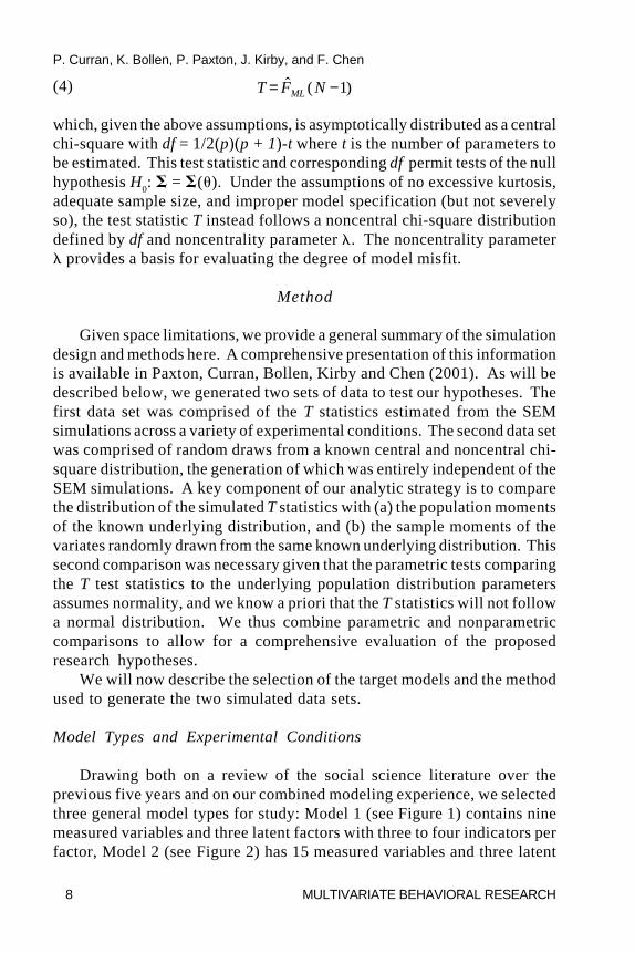
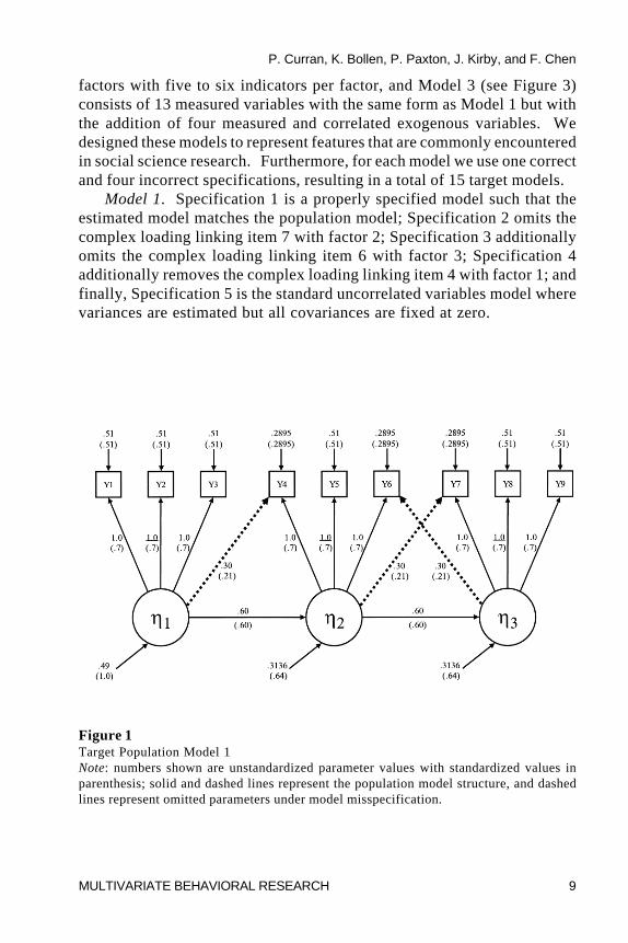
Drawing both on a review of the social science literature over theprevious five years and on our combined modeling experience, we selectedthree general model types for study: Model 1 (see Figure 1) contains ninemeasured variables and three latent factors with three to four indicators perfactor, Model 2 (see Figure 2) has 15 measured variables and three latent
P. Curran, K. Bollen, P. Paxton, J. Kirby, and F. Chen
MULTIVARIATE BEHAVIORAL RESEARCH 9
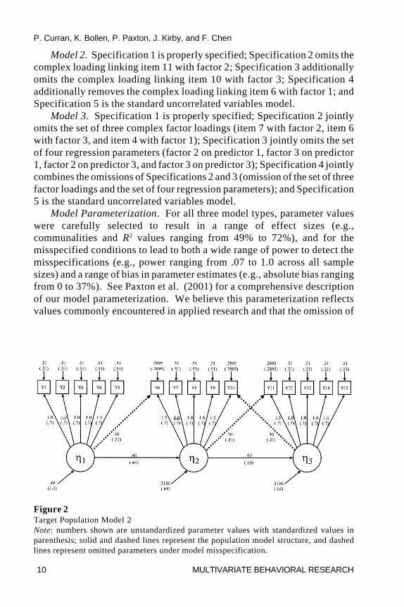
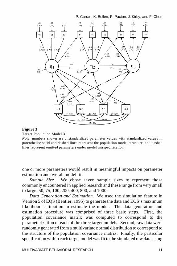
factors with five to six indicators per factor, and Model 3 (see Figure 3)consists of 13 measured variables with the same form as Model 1 but withthe addition of four measured and correlated exogenous variables. Wedesigned these models to represent features that are commonly encounteredin social science research. Furthermore, for each model we use one correctand four incorrect specifications, resulting in a total of 15 target models.
Model 1. Specification 1 is a properly specified model such that theestimated model matches the population model; Specification 2 omits thecomplex loading linking item 7 with factor 2; Specification 3 additionallyomits the complex loading linking item 6 with factor 3; Specification 4additionally removes the complex loading linking item 4 with factor 1; andfinally, Specification 5 is the standard uncorrelated variables model wherevariances are estimated but all covariances are fixed at zero.
Figure 1Target Population Model 1Note: numbers shown are unstandardized parameter values with standardized values inparenthesis; solid and dashed lines represent the population model structure, and dashedlines represent omitted parameters under model misspecification.
P. Curran, K. Bollen, P. Paxton, J. Kirby, and F. Chen
10 MULTIVARIATE BEHAVIORAL RESEARCH
Model 2. Specification 1 is properly specified; Specification 2 omits thecomplex loading linking item 11 with factor 2; Specification 3 additionallyomits the complex loading linking item 10 with factor 3; Specification 4additionally removes the complex loading linking item 6 with factor 1; andSpecification 5 is the standard uncorrelated variables model.
Model 3. Specification 1 is properly specified; Specification 2 jointlyomits the set of three complex factor loadings (item 7 with factor 2, item 6with factor 3, and item 4 with factor 1); Specification 3 jointly omits the setof four regression parameters (factor 2 on predictor 1, factor 3 on predictor1, factor 2 on predictor 3, and factor 3 on predictor 3); Specification 4 jointlycombines the omissions of Specifications 2 and 3 (omission of the set of threefactor loadings and the set of four regression parameters); and Specification5 is the standard uncorrelated variables model.
Model Parameterization. For all three model types, parameter valueswere carefully selected to result in a range of effect sizes (e.g.,communalities and R2 values ranging from 49% to 72%), and for themisspecified conditions to lead to both a wide range of power to detect themisspecifications (e.g., power ranging from .07 to 1.0 across all samplesizes) and a range of bias in parameter estimates (e.g., absolute bias rangingfrom 0 to 37%). See Paxton et al. (2001) for a comprehensive descriptionof our model parameterization. We believe this parameterization reflectsvalues commonly encountered in applied research and that the omission of
Figure 2Target Population Model 2Note: numbers shown are unstandardized parameter values with standardized values inparenthesis; solid and dashed lines represent the population model structure, and dashedlines represent omitted parameters under model misspecification.
P. Curran, K. Bollen, P. Paxton, J. Kirby, and F. Chen
MULTIVARIATE BEHAVIORAL RESEARCH 11
one or more parameters would result in meaningful impacts on parameterestimation and overall model fit.
Sample Size. We chose seven sample sizes to represent thosecommonly encountered in applied research and these range from very smallto large: 50, 75, 100, 200, 400, 800, and 1000.
Data Generation and Estimation. We used the simulation feature inVersion 5 of EQS (Bentler, 1995) to generate the data and EQS’s maximumlikelihood estimation to estimate the model. The data generation andestimation procedure was comprised of three basic steps. First, thepopulation covariance matrix was computed to correspond to theparameterization of each of the three target models. Second, raw data wererandomly generated from a multivariate normal distribution to correspond tothe structure of the population covariance matrix. Finally, the particularspecification within each target model was fit to the simulated raw data using
Figure 3Target Population Model 3Note: numbers shown are unstandardized parameter values with standardized values inparenthesis; solid and dashed lines represent the population model structure, and dashedlines represent omitted parameters under model misspecification.
P. Curran, K. Bollen, P. Paxton, J. Kirby, and F. Chen
12 MULTIVARIATE BEHAVIORAL RESEARCH
ML estimation. We used the population values for each parameter as initialstart values, and we allowed a maximum of 100 iterations to achieveconvergence. This method permitted us to fit a model that differed instructure from the model that generated the data . See Bentler (1995) forfurther details about EQS data generation procedures.
Distribution. We generated data from a multivariate normaldistribution.
Replications. There were a total of 105 experimental conditions (threemodels, five specifications, and seven sample sizes), and we generated up to500 replications for each condition.
Convergence. We eliminated any replication that failed to convergewithin 100 iterations, or did converge but resulted in an out of boundsparameter estimate (e.g., “Heywood Case”) or a linear dependency amongparameters. To maintain 500 replications per condition, we generated aninitial set of up to 650 replications. We then fit the models to the generateddata and selected the first 500 proper solutions, or selected as many propersolutions as existed when the total number of replications was reached. Thisresulted in 500 proper solutions for all properly specified and mostmisspecified experimental conditions, but there were several misspecifiedconditions that resulted in fewer than 500 proper solutions. Of the 105experimental conditions, 82 (78%) contained 500 replications and 23 (22%)contained fewer than 500 replications. Of those 23 conditions containingfewer than 500 replications, the number of replications ranged from 443 to499 with a median of 492, and the smallest number of 443 replications wasfor Model 3, Specification 4, N = 50. Whether improper solutions should beexcluded or removed from the simulation design is a debatable issue. Wechose to exclude improper solutions to mimic the lowered chance of resultswith improper solutions being reported. Fortunately, no differences werefound in any results when including or excluding improper solutions (seeAnderson & Gerbing, 1984, for further discussion of this topic). Elsewherewe have examined the causes and consequences of improper solutions inmore detail ( Chen, Bollen, Paxton, Curran, & Kirby, 2001).
Outcome Measures. The outcome measures of key interest here is thelikelihood ratio test statistic T (commonly referred to as the “model �2”)estimated for each replicated model and the corresponding degrees offreedom for the estimated model. We obtained these values directly fromEQS in which the T statistic is computed as the product of the minimum ofthe ML fit function and N - 1, and the df is computed as the differencebetween the total number of unique variances and covariances minus thetotal number of estimated parameters.
P. Curran, K. Bollen, P. Paxton, J. Kirby, and F. Chen
MULTIVARIATE BEHAVIORAL RESEARCH 13
Simulated Data Drawn from the Noncentral Chi-Square Distribution
Data Generation. A key research question posed here is whether themodel test statistics T computed from the simulated structural equationmodels follow the expected underlying central or noncentral chi-squaredistribution. As part of the empirical evaluation of this question, we generatedadditional simulated data drawn directly from the known population chi-square distributions using Version 7.0 of the SAS data system (SAS Inc.,1999). As mentioned earlier, we did this to allow for nonparametric tests thatdo not assume that the test statistics are normally distributed, a condition thatlikely does not hold here. We generated random variates from expectedpopulation distributions using a combination of the gamma and normaldistribution functions in SAS. When � was zero, this resulted in random drawsfrom the central chi-square distribution; when � was greater than zero, thisresulted in random draws from the noncentral chi-square distribution.
Experimental Conditions. The mean and variance of the central andnoncentral chi-square distributions vary as a function of degrees of freedomand the noncentrality parameter �. Thus, we drew 105 separate samplesfrom 105 different population distributions, one corresponding to each SEMexperimental condition under study.
Replications. To achieve stable sample estimates of the underlyingpopulation distributions, we made 5000 draws for each of the 105experimental conditions. Thus, all means and variances reported below arebased on 5000 independent draws for each experimental condition.
Summary
In sum, we generated two complete sets of data to empirically evaluateour proposed research hypotheses. The first set was comprised of up to 500test statistics T (one drawn from each SEM replication) estimated withineach of 105 experimental conditions; we refer to these data as the SEMsimulations. The second set was comprised of 5000 random draws from105 different population central (for properly specified models) andnoncentral (for misspecified models) chi-square distributions, onedistribution corresponding to each SEM experimental condition under study;we refer to these data as the chi-square simulations. The core of our dataanalytic strategy is (a) the parametric comparison of the sample means andvariances of the T statistics from the SEM simulations with the knownpopulation counterparts, and (b) the nonparametric comparison of the meansand variances of the T statistics from the SEM simulations with the randomchi-square variates drawn from the known population distributions.
P. Curran, K. Bollen, P. Paxton, J. Kirby, and F. Chen
14 MULTIVARIATE BEHAVIORAL RESEARCH
Results
We empirically evaluated the proposed research hypotheses using threerelated methods. First, we computed one-sample z-tests of the sample meanof the SEM test statistics to the corresponding population mean with knownpopulation variance, and we used one-sample �2 tests of the sample varianceof the SEM test statistics to the corresponding population variance. Theseare parametric tests of the null hypothesis that the sample mean and varianceof the SEM test statistics equals the population mean and variance of theexpected underlying distributions, and both tests assume that the populationis normally distributed (Kanji, 1993). Second, because of the assumption ofnormality associated with the parametric tests, a condition that is notexpected to hold here,2 we used the nonparametric Wilcoxon Rank-Sum testof means and Siegel-Tukey test of variances to compare the empiricaldistributions of the SEM statistics with the corresponding empiricaldistributions from the chi-square simulations. The Wilcoxon Rank-Sum testevaluates the hypothesis that two random samples came from twopopulations with the same mean, and the Siegel-Tukey test evaluates thehypothesis that two random samples came from two populations with thesame variance. Both of these nonparametric tests only assume that the twopopulations have continuous frequency distributions (Kanji, 1993, p. 86).Finally, to augment the parametric and nonparametric statistical tests, wecomputed effect sizes based on absolute relative bias (observed value minusexpected value divided by expected value) and considered values of 5% orgreater to indicate meaningful bias. In sum, we utilized parametric tests,nonparametric tests, and measures of effect size to evaluate our researchhypotheses.
Tests of Central Tendency
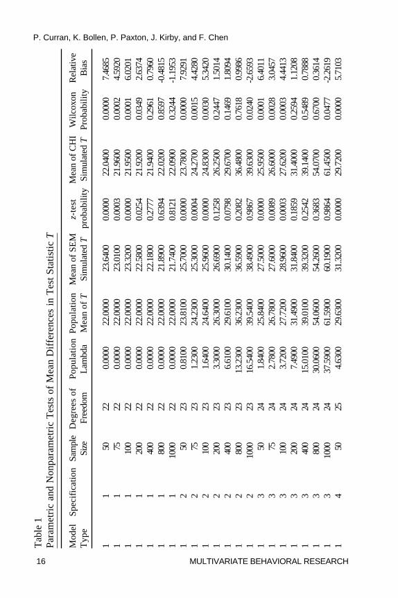
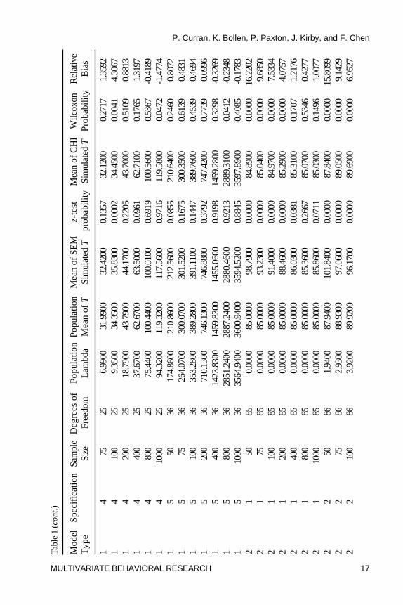
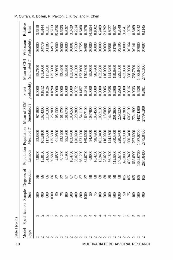
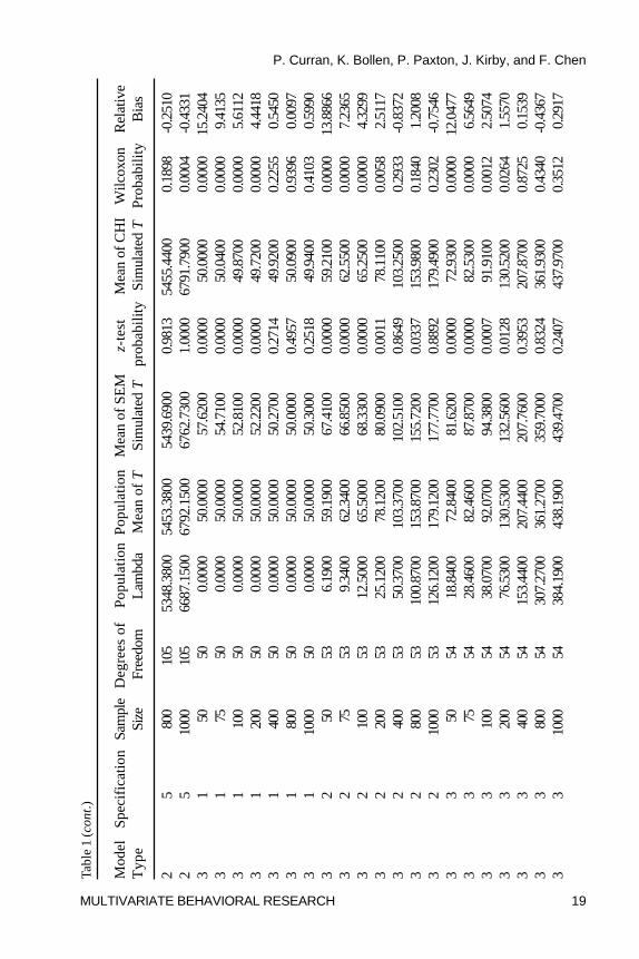
One Sample z-Test. Table 1 presents all summary statistics and theresults of the parametric (z) and nonparametric (Wilcoxon) tests for themeans of the population distribution, the SEM simulations, and the chi-squaresimulations. For each of the 105 experimental conditions, we compared thesample mean of the SEM test statistic T to the mean of the population
2 We do not expect the assumption of normality to hold here because the T statistics areexpected to follow a central or noncentral chi-square distribution which itself is not normal,at least under the conditions studied here. However, 103 of the 105 measures of univariatekurtosis of the sample distributions of T were below 1.0, and the largest value of kurtosiswas 1.1 (Model 3, Specification 1, N = 100). Based on these empirical results, it does notappear that the assumption of normality is excessively violated here.
P. Curran, K. Bollen, P. Paxton, J. Kirby, and F. Chen
MULTIVARIATE BEHAVIORAL RESEARCH 15
distribution that it is expected to follow given a known population variance.To control for inflated familywise error rate stemming from the 105 meancomparisons, we set the per comparison rate to � = .001 to maintain afamilywise rate of approximately � = .10. Using this significance criterion,3 arather clear pattern of results emerges across all conditions: the mean of theSEM test statistics systematically overestimated the mean of the expectedunderlying population distributions at the smaller sample sizes across all threemodel types. For Specifications 1 through 4 (the one proper and threeimproper specifications) of Model 1, this tended to occur at sample sizes of100 and below, and for Specifications 1 through 4 of Models 2 and 3, thistended to occur at sample sizes of 200 and below. Interestingly, there waslittle evidence of bias in the mean estimate for Specification 5 (theuncorrelated variables model) for Model 1, and there was modestoverestimation for Specification 5 of Models 2 and 3, but only at the smallestsample size of 50.
Relative Bias. To further understand these relations in terms of effectsizes, relative bias was computed for all conditions. For Model 1, significantrelative bias in the means (e.g., greater than 5%) was observed at samplesizes of N = 100 and below for the proper specification, at N = 50 for theimproper specifications, and no bias was observed for the uncorrelatedvariables null model. For Model 2, the significant relative bias in the meanswas observed for both the proper and improper specifications at N = 100 andbelow, and again there was no appreciable bias for the null model. Thispattern was also found for Model 3 but only at sample sizes of N = 75 andbelow. In general, the experimental conditions associated with significantrelative bias closely corresponded with those conditions identified using theparametric z-test, but the relative bias results were somewhat moreconservative compared to the parametric results. Thus, based on the 5%relative bias criterion, the means were systematically overestimated at thesmaller sample sizes for the proper and improper model specifications, andthe mean for the null model was unbiased across all sample sizes.
Wilcoxon Rank-Sum Test. The Wilcoxon Rank Sum test compared themean of the SEM test statistics with the mean of the 5000 random variatesdrawn from the corresponding population distribution that the test statisticsare expected to follow. Again, we used this method of comparison given the
3 It could be argued that there are actually 210 total tests (e.g., 105 tests of mean and 105tests of variance), or even 420 total tests given the inclusion of the nonparametric mean andvariance comparisons. We chose to correct for 105 tests because these were the totalnumber of comparisons that focused on one particular parameter within one particularstatistical test. However, we present exact p-values for each individual test so that thereader may make any correction they so desire.
P. Curran, K. Bollen, P. Paxton, J. Kirby, and F. Chen
16 MULTIVARIATE BEHAVIORAL RESEARCH
Tab
le 1
Par
amet
ric
and
Non
para
met
ric
Tes
ts o
f M
ean
Dif
fere
nces
in
Tes
t S
tati
stic
T
Mod
elSp
ecif
icat
ion
Sam
ple
Deg
rees
of
Pop
ulat
ion
Pop
ulat
ion
Mea
n of
SE
Mz-
test
Mea
n of
CH
IW
ilcox
onR
elat
ive
Typ
eSi
ze F
reed
omL
ambd
aM
ean
of T
Sim
ulat
ed T
pro
babi
lity
Sim
ulat
ed T
Prob
abili
tyB
ias
11
5022
0.00
0022
.000
023
.640
00.
0000
22.0
400
0.00
007.
4685
11
7522
0.00
0022
.000
023
.010
00.
0003
21.9
600
0.00
024.
5920
11
100
220.
0000
22.0
000
23.3
200
0.00
0021
.950
00.
0001
6.02
011
120
022
0.00
0022
.000
022
.580
00.
0254
21.9
200
0.03
492.
6374
11
400
220.
0000
22.0
000
22.1
800
0.27
7721
.940
00.
2961
0.79
601
180
022
0.00
0022
.000
021
.890
00.
6394
22.0
200
0.85
97-0
.481
51
110
0022
0.00
0022
.000
021
.740
00.
8121
22.0
900
0.32
44-1
.195
31
250
230.
8100
23.8
100
25.7
000
0.00
0023
.780
00.
0000
7.92
911
275
231.
2300
24.2
300
25.3
000
0.00
0424
.270
00.
0015
4.42
801
210
023
1.64
0024
.640
025
.960
00.
0000
24.8
300
0.00
305.
3420
12
200
233.
3000
26.3
000
26.6
900
0.12
5826
.250
00.
2447
1.50
141
240
023
6.61
0029
.610
030
.140
00.
0798
29.6
700
0.14
691.
8094
12
800
2313
.230
036
.230
036
.590
00.
2082
36.4
800
0.76
180.
9986
12
1000
2316
.540
039
.540
038
.490
00.
9867
39.6
300
0.02
40-2
.659
31
350
241.
8400
25.8
400
27.5
000
0.00
0025
.950
00.
0001
6.40
111
375
242.
7800
26.7
800
27.6
000
0.00
8926
.600
00.
0028
3.04
571
310
024
3.72
0027
.720
028
.960
00.
0003
27.6
200
0.00
034.
4413
13
200
247.
4900
31.4
900
31.8
400
0.18
5931
.400
00.
2594
1.12
081
340
024
15.0
100
39.0
100
39.3
200
0.25
4239
.140
00.
5489
0.78
881
380
024
30.0
600
54.0
600
54.2
600
0.36
8354
.070
00.
6700
0.36
141
310
0024
37.5
900
61.5
900
60.1
900
0.98
6461
.450
00.
0477
-2.2
619
14
5025
4.63
0029
.630
031
.320
00.
0000
29.7
200
0.00
005.
7103
P. Curran, K. Bollen, P. Paxton, J. Kirby, and F. Chen
MULTIVARIATE BEHAVIORAL RESEARCH 17
14
7525
6.99
0031
.990
032
.420
00.
1357
32.1
200
0.27
171.
3592
14
100
259.
3500
34.3
500
35.8
300
0.00
0234
.450
00.
0041
4.30
671
420
025
18.7
900
43.7
900
44.1
700
0.22
0543
.700
00.
5109
0.88
131
440
025
37.6
700
62.6
700
63.5
000
0.09
6162
.710
00.
1765
1.31
971
480
025
75.4
400
100.
4400
100.
0100
0.69
1910
0.56
000.
5367
-0.4
189
14
1000
2594
.320
011
9.32
0011
7.56
000.
9716
119.
5800
0.04
72-1
.477
41
550
3617
4.86
0021
0.86
0021
2.56
000.
0855
210.
6400
0.24
600.
8072
15
7536
264.
0700
300.
0700
301.
5200
0.16
7530
0.35
000.
6139
0.48
311
510
036
353.
2800
389.
2800
391.
1100
0.14
4738
9.76
000.
4539
0.46
941
520
036
710.
1300
746.
1300
746.
8800
0.37
9274
7.42
000.
7739
0.09
961
540
036
1423
.830
014
59.8
300
1455
.060
00.
9198
1459
.280
00.
3298
-0.3
269
15
800
3628
51.2
400
2887
.240
028
80.4
600
0.92
1328
89.3
100
0.04
12-0
.234
81
510
0036
3564
.940
036
00.9
400
3594
.520
00.
8845
3597
.890
00.
4085
-0.1
783
21
5085
0.00
0085
.000
098
.790
00.
0000
84.8
900
0.00
0016
.220
22
175
850.
0000
85.0
000
93.2
300
0.00
0085
.040
00.
0000
9.68
502
110
085
0.00
0085
.000
091
.400
00.
0000
84.9
700
0.00
007.
5334
21
200
850.
0000
85.0
000
88.4
600
0.00
0085
.290
00.
0000
4.07
572
140
085
0.00
0085
.000
086
.030
00.
0381
85.3
100
0.17
071.
2176
21
800
850.
0000
85.0
000
85.3
600
0.26
6785
.070
00.
5346
0.42
772
110
0085
0.00
0085
.000
085
.860
00.
0711
85.0
300
0.14
961.
0077
22
5086
1.94
0087
.940
010
1.84
000.
0000
87.8
400
0.00
0015
.809
92
275
862.
9300
88.9
300
97.0
600
0.00
0089
.050
00.
0000
9.14
292
210
086
3.92
0089
.920
096
.170
00.
0000
89.6
900
0.00
006.
9527
Tabl
e 1
(con
t.)
Mod
elSp
ecif
icat
ion
Sam
ple
Deg
rees
of
Pop
ulat
ion
Pop
ulat
ion
Mea
n of
SE
Mz-
test
Mea
n of
CH
IW
ilcox
onR
elat
ive
Typ
eSi
ze F
reed
omL
ambd
aM
ean
of T
Sim
ulat
ed T
pro
babi
lity
Sim
ulat
ed T
Prob
abili
tyB
ias
P. Curran, K. Bollen, P. Paxton, J. Kirby, and F. Chen
18 MULTIVARIATE BEHAVIORAL RESEARCH
22
200
867.
8800
93.8
800
97.1
900
0.00
0093
.710
00.
0000
3.52
102
240
086
15.8
100
101.
8100
102.
4300
0.18
1210
1.90
000.
4779
0.61
442
280
086
31.6
500
117.
6500
118.
6300
0.10
2611
7.27
000.
1185
0.83
312
210
0086
39.5
800
125.
5800
126.
3000
0.18
9012
5.39
000.
4919
0.57
132
350
874.
0500
91.0
500
105.
1300
0.00
0090
.960
00.
0000
15.4
536
23
7587
6.12
0093
.120
010
1.17
000.
0000
93.4
200
0.00
008.
6425
23
100
878.
1900
95.1
900
101.
6700
0.00
0095
.330
00.
0000
6.80
972
320
087
16.4
700
103.
4700
106.
6500
0.00
0010
3.48
000.
0001
3.07
292
340
087
33.0
200
120.
0200
120.
2800
0.36
7212
0.19
000.
7530
0.22
142
380
087
66.1
200
153.
1200
154.
1100
0.14
5715
3.08
000.
2725
0.64
602
310
0087
82.6
700
169.
6700
169.
7100
0.48
1417
0.13
000.
6981
0.02
762
450
886.
9000
94.9
000
108.
7800
0.00
0095
.060
00.
0000
14.6
254
24
7588
10.4
200
98.4
200
106.
4500
0.00
0098
.490
00.
0000
8.16
022
410
088
13.9
400
101.
9400
108.
3100
0.00
0010
2.25
000.
0000
6.24
892
420
088
28.0
200
116.
0200
118.
5000
0.00
0511
6.00
000.
0039
2.13
922
440
088
56.1
800
144.
1800
144.
7500
0.26
3814
4.34
000.
5801
0.39
272
480
088
112.
5000
200.
5000
201.
2600
0.25
0619
9.63
000.
1769
0.37
572
410
0088
140.
6700
228.
6700
229.
3200
0.29
6322
9.16
000.
9196
0.28
482
550
105
328.
0000
433.
0000
449.
3800
0.00
0043
3.05
000.
0000
3.78
412
575
105
495.
3400
600.
3400
606.
5100
0.00
1659
8.93
000.
0164
1.02
762
510
010
566
2.69
0076
7.69
0077
4.19
000.
0033
768.
7500
0.01
410.
8469
25
200
105
1332
.070
014
37.0
700
1437
.130
00.
4928
1438
.040
00.
7900
0.00
422
540
010
526
70.8
400
2775
.840
027
79.0
200
0.24
8127
77.1
000
0.70
970.
1145
Tabl
e 1
(con
t.)
Mod
elSp
ecif
icat
ion
Sam
ple
Deg
rees
of
Pop
ulat
ion
Pop
ulat
ion
Mea
n of
SE
Mz-
test
Mea
n of
CH
IW
ilcox
onR
elat
ive
Typ
eSi
ze F
reed
omL
ambd
aM
ean
of T
Sim
ulat
ed T
pro
babi
lity
Sim
ulat
ed T
Prob
abili
tyB
ias
P. Curran, K. Bollen, P. Paxton, J. Kirby, and F. Chen
MULTIVARIATE BEHAVIORAL RESEARCH 19
25
800
105
5348
.380
054
53.3
800
5439
.690
00.
9813
5455
.440
00.
1898
-0.2
510
25
1000
105
6687
.150
067
92.1
500
6762
.730
01.
0000
6791
.790
00.
0004
-0.4
331
31
5050
0.00
0050
.000
057
.620
00.
0000
50.0
000
0.00
0015
.240
43
175
500.
0000
50.0
000
54.7
100
0.00
0050
.040
00.
0000
9.41
353
110
050
0.00
0050
.000
052
.810
00.
0000
49.8
700
0.00
005.
6112
31
200
500.
0000
50.0
000
52.2
200
0.00
0049
.720
00.
0000
4.44
183
140
050
0.00
0050
.000
050
.270
00.
2714
49.9
200
0.22
550.
5450
31
800
500.
0000
50.0
000
50.0
000
0.49
5750
.090
00.
9396
0.00
973
110
0050
0.00
0050
.000
050
.300
00.
2518
49.9
400
0.41
030.
5990
32
5053
6.19
0059
.190
067
.410
00.
0000
59.2
100
0.00
0013
.886
63
275
539.
3400
62.3
400
66.8
500
0.00
0062
.550
00.
0000
7.23
653
210
053
12.5
000
65.5
000
68.3
300
0.00
0065
.250
00.
0000
4.32
993
220
053
25.1
200
78.1
200
80.0
900
0.00
1178
.110
00.
0058
2.51
173
240
053
50.3
700
103.
3700
102.
5100
0.86
4910
3.25
000.
2933
-0.8
372
32
800
5310
0.87
0015
3.87
0015
5.72
000.
0337
153.
9800
0.18
401.
2008
32
1000
5312
6.12
0017
9.12
0017
7.77
000.
8892
179.
4900
0.23
02-0
.754
63
350
5418
.840
072
.840
081
.620
00.
0000
72.9
300
0.00
0012
.047
73
375
5428
.460
082
.460
087
.870
00.
0000
82.5
300
0.00
006.
5649
33
100
5438
.070
092
.070
094
.380
00.
0007
91.9
100
0.00
122.
5074
33
200
5476
.530
013
0.53
0013
2.56
000.
0128
130.
5200
0.02
641.
5570
33
400
5415
3.44
0020
7.44
0020
7.76
000.
3953
207.
8700
0.87
250.
1539
33
800
5430
7.27
0036
1.27
0035
9.70
000.
8324
361.
9300
0.43
40-0
.436
73
310
0054
384.
1900
438.
1900
439.
4700
0.24
0743
7.97
000.
3512
0.29
17
Tabl
e 1
(con
t.)
Mod
elSp
ecif
icat
ion
Sam
ple
Deg
rees
of
Pop
ulat
ion
Pop
ulat
ion
Mea
n of
SE
Mz-
test
Mea
n of
CH
IW
ilcox
onR
elat
ive
Typ
eSi
ze F
reed
omL
ambd
aM
ean
of T
Sim
ulat
ed T
pro
babi
lity
Sim
ulat
ed T
Prob
abili
tyB
ias
P. Curran, K. Bollen, P. Paxton, J. Kirby, and F. Chen
20 MULTIVARIATE BEHAVIORAL RESEARCH
34
5057
26.3
100
83.3
100
92.1
000
0.00
0083
.490
00.
0000
10.5
594
34
7557
39.7
300
96.7
300
101.
6000
0.00
0096
.770
00.
0000
5.03
543
410
057
53.1
500
110.
1500
112.
4800
0.00
2010
9.86
000.
0015
2.11
793
420
057
106.
8400
163.
8400
165.
3500
0.07
3316
4.29
000.
3195
0.92
273
440
057
214.
2200
271.
2200
270.
1000
0.78
7527
0.99
000.
4441
-0.4
103
34
800
5742
8.97
0048
5.97
0048
6.44
000.
4022
485.
8500
0.58
370.
0976
34
1000
5753
6.34
0059
3.34
0059
2.83
000.
5954
593.
1200
0.74
77-0
.086
63
550
7826
8.81
0034
6.81
0036
1.20
000.
0000
346.
9100
0.00
004.
1472
35
7578
405.
9600
483.
9600
492.
1800
0.00
0048
4.22
000.
0018
1.69
753
510
078
543.
1100
621.
1100
623.
7800
0.10
8262
1.08
000.
3759
0.42
993
520
078
1091
.710
011
69.7
100
1174
.380
00.
0606
1168
.690
00.
1011
0.39
893
540
078
2188
.910
022
66.9
100
2271
.550
00.
1364
2267
.210
00.
3924
0.20
443
580
078
4383
.310
044
61.3
100
4468
.900
00.
1014
4460
.530
00.
1779
0.17
003
510
0078
5480
.510
055
58.5
100
5567
.340
00.
0924
5560
.000
00.
2206
0.15
87
Mod
elSp
ecif
icat
ion
Sam
ple
Deg
rees
of
Pop
ulat
ion
Pop
ulat
ion
Mea
n of
SE
Mz-
test
Mea
n of
CH
IW
ilcox
onR
elat
ive
Typ
eSi
ze F
reed
omL
ambd
aM
ean
of T
Sim
ulat
ed T
pro
babi
lity
Sim
ulat
ed T
Prob
abili
tyB
ias
Tabl
e 1
(con
t.)
P. Curran, K. Bollen, P. Paxton, J. Kirby, and F. Chen
MULTIVARIATE BEHAVIORAL RESEARCH 21
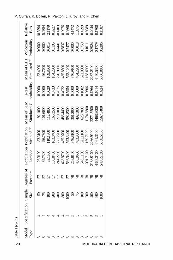
likely failure of the T statistics to meet the assumption of normality requiredby the z-test. As expected, the nonparametric tests tended to demonstratelower power relative to the parametric counterparts. However, nearlywithout exception, every condition for which a meaningful difference resultsusing the parametric tests, this same condition is identified in thenonparametric tests (based on the corrected � = .001).
Summary of Tests of Central Tendency. Based on the correctedsignificance levels of the parametric and nonparametric tests as well as themagnitude of relative bias, we concluded that the mean of the SEM teststatistics consistently overestimated the mean of the expected underlyingpopulation distribution for Specifications 1 through 4 for all three model types(the properly specified and three misspecified conditions), but only at thesmallest sample sizes (e.g., 100 to 200 and below). At samples above 200,we found no appreciable bias across any condition. Further, we found nosignificant overestimation of the population mean for Specification 5 (theuncorrelated variables model) for any model type at any sample size.
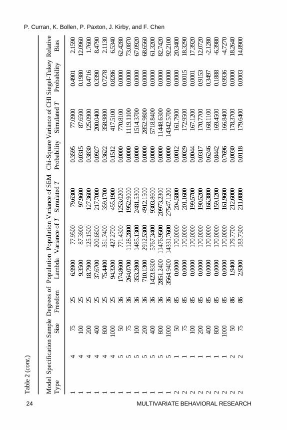
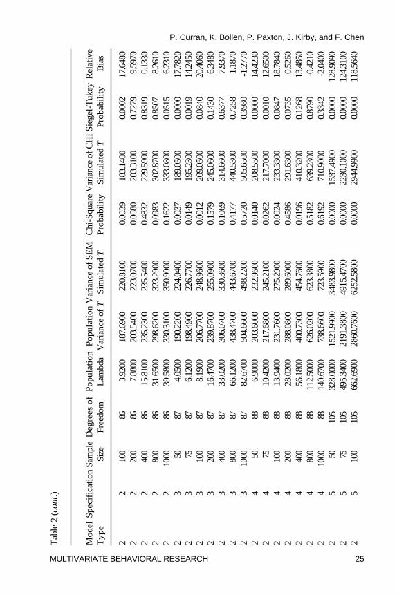
Tests of Dispersion
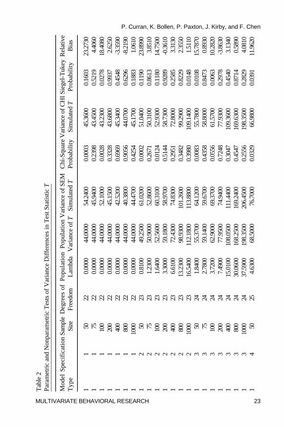
One Sample �2-Test. Table 2 presents all summary statistics, parametric(�2) and nonparametric (Siegel-Tukey) tests, and relative bias for the variancesof the population distribution, the SEM simulations, and the chi-squaresimulations. Again using a per comparison rate of � = .001 to control for multipletesting, the variance of the T statistics for Model 1 only significantly varied fromthe expected population value at the smallest sample size for the properlyspecified and the most minor improper specification (Specifications 1 and 2); incontrast, the variance was significantly overestimated across all sample sizesfor the uncorrelated variable baseline model (Specification 5). A similar patternof results was found for both Model 2 and Model 3. Thus, although there wasevidence of significant overestimation of the sample variance of T relative to theexpected underlying distribution at N = 50 for the proper and minor improperspecifications, the variance of the uncorrelated variable baseline model wassignificantly overestimated at every sample size for every model type even usingthe adjusted � = .001 per comparison error rate.
Relative Bias. Unlike the tests of central tendency that indicated alarger number of biased conditions based on the parametric test resultscompared to the relative bias results, for the tests of dispersion a largernumber of biased conditions were identified based upon the relative biasresults compared to the parametric test results. For Specifications 1 through4 for all three model types, the variance of the SEM test statisticsoverestimated the expected variance of the population distributions at the
P. Curran, K. Bollen, P. Paxton, J. Kirby, and F. Chen
22 MULTIVARIATE BEHAVIORAL RESEARCH
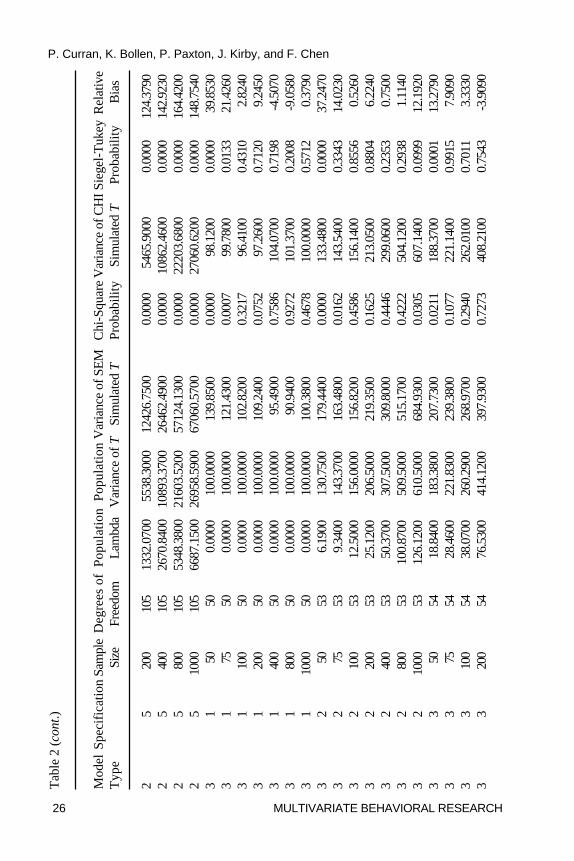
smaller sample sizes. Relative bias exceeded 5% at samples of N = 100and below for Model 1,4 at about N = 200 and below for Model 2, and atabout N = 75 and below for Model 3. Indeed, at the smallest sample sizeof N = 50, relative bias ranged from 12% up to 39% indicating substantialoverestimation of the corresponding population parameter.5 Of key interestis the finding that for Specification 5 (the uncorrelated variables model), thesample variance of the SEM test statistics significantly overestimated thepopulation counterpart at every sample size across all three model types withrelative bias ranging from a minimum of 32% to a remarkable 164%. Indeed,for Model 2, bias was 120% or higher across all sample sizes. Thus, for theuncorrelated variables model, there was not one instance in which the sampleestimates of the SEM test statistics showed evidence of following thedispersion of the expected noncentral chi-square population distribution.
Siegel-Tukey Test. As with the z-test of the means, the parametric �2
test of the variances also assumes normality thus necessitating the use of thenonparametric equivalents. The Siegel-Tukey nonparametric test ofvariance (Kanji, 1993, p. 87) compared the variance of the SEM teststatistics and the variance of the N = 5000 random variates drawn from theexpected underlying population distribution, and this test only assumes thatthe population distributions are continuous. In general, as was found with theWilcoxon Rank-Sum test of central tendency, the results of the Siegel-Tukeytest of dispersion closely corresponded with those of the �2 test, althoughagain there is some evidence of the lower power of the nonparametric test.In general, the Siegel-Tukey results indicated overestimation of the varianceat the smallest sample size for nearly all of the properly and improperlyspecified models, and indicated significant overestimation at all sample sizesfor all three model types for the uncorrelated variable baseline model.
Summary of Tests of Dispersion. Results from the parametric andnonparametric tests in combination with the magnitude of the absoluterelative bias lead us to two key patterns of results. First, for Specifications
4 An odd pattern of findings was evident for the first four Specifications of Model 1 at N = 75in which the estimated variance of the SEM test statistics was smaller at N = 75 comparedto the N = 50 and N = 100 conditions. We suspected that this was an error in datageneration, but extensive exploration of these conditions coupled with the generation ofadditional data revealed no errors. We found that there is much sampling variability in theestimation of the variance of the SEM test statistics at the smaller sample sizes, and thesomewhat odd pattern of results for this one particular condition is most likely attributableto this random variability.5 One interesting finding to note is that at N = 400 and N = 800 of Specification 3 of Model3, the relative bias was actually a negative value (both approximately -18%). This findingwas not predicted, but also was not consistent across model or specification. It is thus notimmediately clear what this limited evidence of underestimation of variance implies, ifanything at all.
P. Curran, K. Bollen, P. Paxton, J. Kirby, and F. Chen
MULTIVARIATE BEHAVIORAL RESEARCH 23
Tab
le 2
Para
met
ric
and
Non
para
met
ric
Tes
ts o
f V
aria
nce
Dif
fere
nces
in T
est S
tatis
tic T
Mod
elSp
ecif
icat
ion
Sam
ple
Deg
rees
of
Pop
ulat
ion
Pop
ulat
ion
Var
ianc
e of
SE
MC
hi-S
quar
eV
aria
nce
of C
HI
Sieg
el-T
ukey
Rel
ativ
eT
ype
Size
Free
dom
Lam
bda
Var
ianc
e of
TSi
mul
ated
TPr
obab
ility
Sim
ulat
ed T
Prob
abili
tyB
ias
11
5022
0.00
0044
.000
054
.240
00.
0003
45.3
600
0.16
0323
.273
01
175
220.
0000
44.0
000
45.9
400
0.23
9843
.450
00.
5219
4.40
601
110
022
0.00
0044
.000
052
.100
00.
0028
43.2
300
0.02
7818
.408
01
120
022
0.00
0044
.000
045
.150
00.
3328
43.6
800
0.99
372.
6250
11
400
220.
0000
44.0
000
42.5
200
0.69
6945
.340
00.
4548
-3.3
590
11
800
220.
0000
44.0
000
40.3
800
0.90
5644
.070
00.
6296
-8.2
190
11
1000
220.
0000
44.0
000
44.4
700
0.42
5445
.170
00.
1883
1.06
101
250
230.
8100
49.2
500
61.0
200
0.00
0251
.040
00.
1190
23.8
990
12
7523
1.23
0050
.900
052
.860
00.
2671
50.3
100
0.86
133.
8510
12
100
231.
6400
52.5
600
60.3
100
0.01
2452
.930
00.
1180
14.7
500
12
200
233.
3000
59.1
800
58.9
700
0.51
4458
.730
00.
9289
-0.3
610
12
400
236.
6100
72.4
300
74.8
300
0.29
5172
.800
00.
2585
3.31
301
280
023
13.2
300
98.9
300
101.
2600
0.34
8299
.290
00.
8229
2.35
501
210
0023
16.5
400
112.
1800
113.
8800
0.39
8010
9.14
000.
0148
1.51
101
350
241.
8400
55.3
700
64.1
200
0.00
8355
.780
00.
0108
15.7
870
13
7524
2.78
0059
.140
059
.670
00.
4358
58.8
000
0.84
730.
8930
13
100
243.
7200
62.9
000
69.3
700
0.05
5661
.570
00.
0063
10.2
820
13
200
247.
4900
77.9
500
74.9
400
0.72
4877
.930
00.
2978
-3.8
630
13
400
2415
.010
010
8.05
0011
1.44
000.
3047
109.
3600
0.45
403.
1340
13
800
2430
.060
016
8.25
0016
9.24
000.
4547
169.
6300
0.87
140.
5890
13
1000
2437
.590
019
8.35
0020
6.45
000.
2556
198.
3500
0.28
294.
0810
14
5025
4.63
0068
.500
076
.700
00.
0329
66.9
800
0.03
9111
.962
0
P. Curran, K. Bollen, P. Paxton, J. Kirby, and F. Chen
24 MULTIVARIATE BEHAVIORAL RESEARCH
Mod
elSp
ecif
icat
ion
Sam
ple
Deg
rees
of
Pop
ulat
ion
Pop
ulat
ion
Var
ianc
e of
SE
MC
hi-S
quar
eV
aria
nce
of C
HI
Sieg
el-T
ukey
Rel
ativ
eT
ype
Size
Free
dom
Lam
bda
Var
ianc
e of
TSi
mul
ated
TPr
obab
ility
Sim
ulat
ed T
Prob
abili
tyB
ias
14
7525
6.99
0077
.950
079
.630
00.
3595
77.0
900
0.49
012.
1590
14
100
259.
3500
87.3
900
97.9
600
0.03
1587
.650
00.
1980
12.0
960
14
200
2518
.790
012
5.15
0012
7.36
000.
3830
125.
0900
0.47
161.
7600
14
400
2537
.670
020
0.68
0021
7.70
000.
0927
200.
0400
0.33
908.
4790
14
800
2575
.440
035
1.74
0035
9.17
000.
3622
358.
9800
0.72
782.
1130
14
1000
2594
.320
042
7.27
0045
5.19
000.
1512
417.
5100
0.82
866.
5340
15
5036
174.
8600
771.
4300
1253
.020
00.
0000
770.
8100
0.00
0062
.428
01
575
3626
4.07
0011
28.2
800
1952
.900
00.
0000
1119
.110
00.
0000
73.0
870
15
100
3635
3.28
0014
85.1
300
2481
.530
00.
0000
1514
.370
00.
0000
67.0
920
15
200
3671
0.13
0029
12.5
300
4912
.150
00.
0000
2852
.980
00.
0000
68.6
560
15
400
3614
23.8
300
5767
.340
093
03.8
600
0.00
0057
18.8
400
0.00
0061
.320
01
580
036
2851
.240
011
476.
9500
2097
3.23
000.
0000
1144
8.63
000.
0000
82.7
420
15
1000
3635
64.9
400
1433
1.76
0027
547.
1200
0.00
0014
342.
5700
0.00
0092
.210
02
150
850.
0000
170.
0000
204.
5800
0.00
1216
1.79
000.
0000
20.3
400
21
7585
0.00
0017
0.00
0020
1.16
000.
0029
172.
9500
0.00
1518
.329
02
110
085
0.00
0017
0.00
0019
9.57
000.
0044
167.
1200
0.00
0117
.392
02
120
085
0.00
0017
0.00
0019
0.52
000.
0317
170.
7700
0.91
5312
.072
02
140
085
0.00
0017
0.00
0016
6.38
000.
6246
168.
1100
0.34
97-2
.128
02
180
085
0.00
0017
0.00
0015
9.12
000.
8442
169.
4500
0.18
88-6
.398
02
110
0085
0.00
0017
0.00
0016
1.96
000.
7696
166.
8400
0.99
36-4
.727
02
250
861.
9400
179.
7700
212.
6000
0.00
3017
8.37
000.
0000
18.2
640
22
7586
2.93
0018
3.73
0021
1.08
000.
0118
179.
6400
0.00
0314
.890
0
Tab
le 2
(co
nt.)
P. Curran, K. Bollen, P. Paxton, J. Kirby, and F. Chen
MULTIVARIATE BEHAVIORAL RESEARCH 25
Mod
elSp
ecif
icat
ion
Sam
ple
Deg
rees
of
Pop
ulat
ion
Pop
ulat
ion
Var
ianc
e of
SE
MC
hi-S
quar
eV
aria
nce
of C
HI
Sieg
el-T
ukey
Rel
ativ
eT
ype
Size
Free
dom
Lam
bda
Var
ianc
e of
TSi
mul
ated
TPr
obab
ility
Sim
ulat
ed T
Prob
abili
tyB
ias
22
100
863.
9200
187.
6900
220.
8100
0.00
3918
3.14
000.
0002
17.6
480
22
200
867.
8800
203.
5400
223.
0700
0.06
8020
3.31
000.
7279
9.59
702
240
086
15.8
100
235.
2300
235.
5400
0.48
3222
9.59
000.
8319
0.13
302
280
086
31.6
500
298.
6200
323.
2900
0.09
8330
2.87
000.
8507
8.26
102
210
0086
39.5
800
330.
3100
350.
9000
0.16
2233
3.08
000.
0515
6.23
102
350
874.
0500
190.
2200
224.
0400
0.00
3718
9.05
000.
0000
17.7
820
23
7587
6.12
0019
8.49
0022
6.77
000.
0149
195.
2300
0.00
1914
.245
02
310
087
8.19
0020
6.77
0024
8.96
000.
0012
209.
0500
0.08
4020
.406
02
320
087
16.4
700
239.
8700
255.
0900
0.15
7924
5.06
000.
1430
6.34
802
340
087
33.0
200
306.
0700
330.
3600
0.10
6931
4.66
000.
6377
7.93
702
380
087
66.1
200
438.
4700
443.
6700
0.41
7744
0.53
000.
7258
1.18
702
310
0087
82.6
700
504.
6600
498.
2200
0.57
2050
5.65
000.
3980
-1.2
770
24
5088
6.90
0020
3.60
0023
2.96
000.
0140
208.
5500
0.00
0014
.423
02
475
8810
.420
021
7.68
0024
5.21
000.
0262
217.
7000
0.00
1012
.650
02
410
088
13.9
400
231.
7600
275.
2900
0.00
2423
3.33
000.
0847
18.7
840
24
200
8828
.020
028
8.08
0028
9.60
000.
4586
291.
6300
0.07
350.
5260
24
400
8856
.180
040
0.73
0045
4.76
000.
0196
410.
3200
0.12
6813
.485
02
480
088
112.
5000
626.
0200
623.
3800
0.51
8263
9.23
000.
8790
-0.4
210
24
1000
8814
0.67
0073
8.66
0072
3.59
000.
6192
710.
9000
0.33
42-2
.040
02
550
105
328.
0000
1521
.990
034
83.9
800
0.00
0015
37.4
900
0.00
0012
8.90
902
575
105
495.
3400
2191
.380
049
15.4
700
0.00
0022
30.1
000
0.00
0012
4.31
002
510
010
566
2.69
0028
60.7
600
6252
.580
00.
0000
2944
.990
00.
0000
118.
5640
Tab
le 2
(co
nt.)
P. Curran, K. Bollen, P. Paxton, J. Kirby, and F. Chen
26 MULTIVARIATE BEHAVIORAL RESEARCH
Mod
elSp
ecif
icat
ion
Sam
ple
Deg
rees
of
Pop
ulat
ion
Pop
ulat
ion
Var
ianc
e of
SE
MC
hi-S
quar
eV
aria
nce
of C
HI
Sieg
el-T
ukey
Rel
ativ
eT
ype
Size
Free
dom
Lam
bda
Var
ianc
e of
TSi
mul
ated
TPr
obab
ility
Sim
ulat
ed T
Prob
abili
tyB
ias
25
200
105
1332
.070
055
38.3
000
1242
6.75
000.
0000
5465
.900
00.
0000
124.
3790
25
400
105
2670
.840
010
893.
3700
2646
2.49
000.
0000
1086
2.46
000.
0000
142.
9230
25
800
105
5348
.380
021
603.
5200
5712
4.13
000.
0000
2220
3.68
000.
0000
164.
4200
25
1000
105
6687
.150
026
958.
5900
6706
0.57
000.
0000
2706
0.62
000.
0000
148.
7540
31
5050
0.00
0010
0.00
0013
9.85
000.
0000
98.1
200
0.00
0039
.853
03
175
500.
0000
100.
0000
121.
4300
0.00
0799
.780
00.
0133
21.4
260
31
100
500.
0000
100.
0000
102.
8200
0.32
1796
.410
00.
4310
2.82
403
120
050
0.00
0010
0.00
0010
9.24
000.
0752
97.2
600
0.71
209.
2450
31
400
500.
0000
100.
0000
95.4
900
0.75
8610
4.07
000.
7198
-4.5
070
31
800
500.
0000
100.
0000
90.9
400
0.92
7210
1.37
000.
2008
-9.0
580
31
1000
500.
0000
100.
0000
100.
3800
0.46
7810
0.00
000.
5712
0.37
903
250
536.
1900
130.
7500
179.
4400
0.00
0013
3.48
000.
0000
37.2
470
32
7553
9.34
0014
3.37
0016
3.48
000.
0162
143.
5400
0.33
4314
.023
03
210
053
12.5
000
156.
0000
156.
8200
0.45
8615
6.14
000.
8556
0.52
603
220
053
25.1
200
206.
5000
219.
3500
0.16
2521
3.05
000.
8804
6.22
403
240
053
50.3
700
307.
5000
309.
8000
0.44
4629
9.06
000.
2353
0.75
003
280
053
100.
8700
509.
5000
515.
1700
0.42
2250
4.12
000.
2938
1.11
403
210
0053
126.
1200
610.
5000
684.
9300
0.03
0560
7.14
000.
0999
12.1
920
33
5054
18.8
400
183.
3800
207.
7300
0.02
1118
8.37
000.
0001
13.2
790
33
7554
28.4
600
221.
8300
239.
3800
0.10
7722
1.14
000.
9915
7.90
903
310
054
38.0
700
260.
2900
268.
9700
0.29
4026
2.01
000.
7011
3.33
303
320
054
76.5
300
414.
1200
397.
9300
0.72
7340
8.21
000.
7543
-3.9
090
Tab
le 2
(co
nt.)
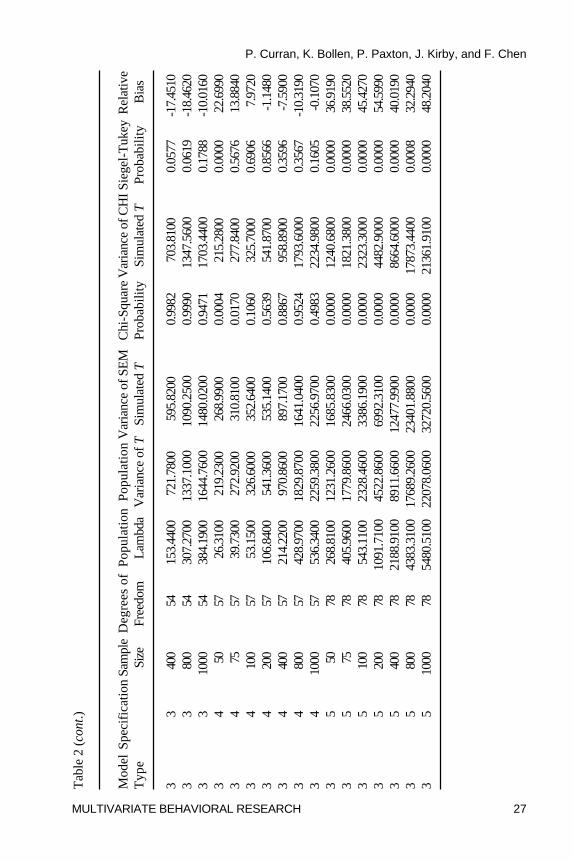
P. Curran, K. Bollen, P. Paxton, J. Kirby, and F. Chen
MULTIVARIATE BEHAVIORAL RESEARCH 27
Mod
elSp
ecif
icat
ion
Sam
ple
Deg
rees
of
Pop
ulat
ion
Pop
ulat
ion
Var
ianc
e of
SE
MC
hi-S
quar
eV
aria
nce
of C
HI
Sieg
el-T
ukey
Rel
ativ
eT
ype
Size
Free
dom
Lam
bda
Var
ianc
e of
TSi
mul
ated
TPr
obab
ility
Sim
ulat
ed T
Prob
abili
tyB
ias
33
400
5415
3.44
0072
1.78
0059
5.82
000.
9982
703.
8100
0.05
77-1
7.45
103
380
054
307.
2700
1337
.100
010
90.2
500
0.99
9013
47.5
600
0.06
19-1
8.46
203
310
0054
384.
1900
1644
.760
014
80.0
200
0.94
7117
03.4
400
0.17
88-1
0.01
603
450
5726
.310
021
9.23
0026
8.99
000.
0004
215.
2800
0.00
0022
.699
03
475
5739
.730
027
2.92
0031
0.81
000.
0170
277.
8400
0.56
7613
.884
03
410
057
53.1
500
326.
6000
352.
6400
0.10
6032
5.70
000.
6906
7.97
203
420
057
106.
8400
541.
3600
535.
1400
0.56
3954
1.87
000.
8566
-1.1
480
34
400
5721
4.22
0097
0.86
0089
7.17
000.
8867
958.
8900
0.35
96-7
.590
03
480
057
428.
9700
1829
.870
016
41.0
400
0.95
2417
93.6
000
0.35
67-1
0.31
903
410
0057
536.
3400
2259
.380
022
56.9
700
0.49
8322
34.9
800
0.16
05-0
.107
03
550
7826
8.81
0012
31.2
600
1685
.830
00.
0000
1240
.680
00.
0000
36.9
190
35
7578
405.
9600
1779
.860
024
66.0
300
0.00
0018
21.3
800
0.00
0038
.552
03
510
078
543.
1100
2328
.460
033
86.1
900
0.00
0023
23.3
000
0.00
0045
.427
03
520
078
1091
.710
045
22.8
600
6992
.310
00.
0000
4482
.900
00.
0000
54.5
990
35
400
7821
88.9
100
8911
.660
012
477.
9900
0.00
0086
64.6
000
0.00
0040
.019
03
580
078
4383
.310
017
689.
2600
2340
1.88
000.
0000
1787
3.44
000.
0008
32.2
940
35
1000
7854
80.5
100
2207
8.06
0032
720.
5600
0.00
0021
361.
9100
0.00
0048
.204
0
Tab
le 2
(co
nt.)
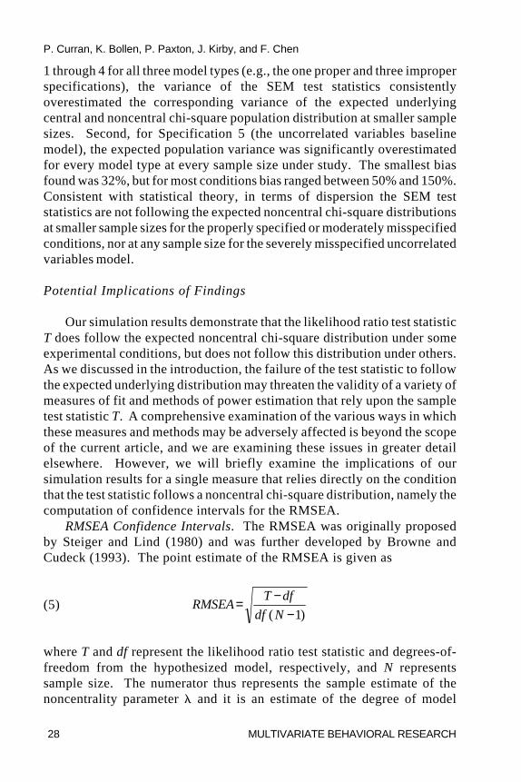
P. Curran, K. Bollen, P. Paxton, J. Kirby, and F. Chen
28 MULTIVARIATE BEHAVIORAL RESEARCH
1 through 4 for all three model types (e.g., the one proper and three improperspecifications), the variance of the SEM test statistics consistentlyoverestimated the corresponding variance of the expected underlyingcentral and noncentral chi-square population distribution at smaller samplesizes. Second, for Specification 5 (the uncorrelated variables baselinemodel), the expected population variance was significantly overestimatedfor every model type at every sample size under study. The smallest biasfound was 32%, but for most conditions bias ranged between 50% and 150%.Consistent with statistical theory, in terms of dispersion the SEM teststatistics are not following the expected noncentral chi-square distributionsat smaller sample sizes for the properly specified or moderately misspecifiedconditions, nor at any sample size for the severely misspecified uncorrelatedvariables model.
Potential Implications of Findings
Our simulation results demonstrate that the likelihood ratio test statisticT does follow the expected noncentral chi-square distribution under someexperimental conditions, but does not follow this distribution under others.As we discussed in the introduction, the failure of the test statistic to followthe expected underlying distribution may threaten the validity of a variety ofmeasures of fit and methods of power estimation that rely upon the sampletest statistic T. A comprehensive examination of the various ways in whichthese measures and methods may be adversely affected is beyond the scopeof the current article, and we are examining these issues in greater detailelsewhere. However, we will briefly examine the implications of oursimulation results for a single measure that relies directly on the conditionthat the test statistic follows a noncentral chi-square distribution, namely thecomputation of confidence intervals for the RMSEA.
RMSEA Confidence Intervals. The RMSEA was originally proposedby Steiger and Lind (1980) and was further developed by Browne andCudeck (1993). The point estimate of the RMSEA is given as
(5) RMSEAT df
df N= −
−( )1
where T and df represent the likelihood ratio test statistic and degrees-of-freedom from the hypothesized model, respectively, and N representssample size. The numerator thus represents the sample estimate of thenoncentrality parameter � and it is an estimate of the degree of model
P. Curran, K. Bollen, P. Paxton, J. Kirby, and F. Chen
MULTIVARIATE BEHAVIORAL RESEARCH 29
misspecification. A unique characteristic of the RMSEA is that, under theassumptions that lead the test statistic to follow a noncentral chi-squaredistribution, the sampling distribution is known. This allows for thecomputation of confidence intervals (CIs) around the point estimate. TheCIs for the RMSEA are computed using appropriate upper and lowerpercentile limits of a noncentral chi-square distribution for given degrees-of-freedom and noncentrality parameter � (see Equation 14, Browne &Cudeck, 1993). The CIs are asymmetric around the point estimate and rangefrom zero to positive infinity.
A key condition for the computation of these CIs is that the test statisticT from the tested model follows a noncentral chi-square distribution. Oursimulation results suggest that T does indeed follow a noncentral chi-squaredistribution under some experimental conditions, but not under others. Tobriefly examine the potential impact of these findings on the computation ofthe CIs for the RMSEA, we compared the percent of sample CIs from theSEM simulations that covered the known population RMSEA value for twoconditions under which we found T to follow a noncentral chi-squaredistribution and for two conditions under which it did not. Under conditionsin which the test statistic follows the population noncentral chi-squaredistribution, we expect that approximately 90% of the 90% CIs would coverthe known population value of the RMSEA.
Recall that the simulation results indicated that the likelihood ratio teststatistic T closely followed the noncentral chi-square distribution in terms ofboth central tendency and dispersion for the moderately misspecified Model3 (the full SEM), Specification 2 (omitting three cross loadings) at N = 400and N = 800. For Specification 2 of Model 3, 91% and 90% of the sample90% CIs covered the population RMSEA value for N = 400 and N = 800,respectively. Thus, under conditions in which T does follow the expectedunderlying distribution, the 90% CIs appear to be covering the populationRMSEA at the expected rate. In contrast, recall that the simulated teststatistics failed to follow a noncentral chi-square distribution for the sameModel 3, Specification 2 at N = 50 and N = 75 in terms of both centraltendency and dispersion. Here, 79% and 86% of the sample 90% CIscovered the population RMSEA value for N = 50 and N = 75, respectively.Thus, under experimental conditions in which T does not follow the expectednoncentral chi-square distribution, the computed CIs based on this underlyingdistribution are not covering the population parameter at the expected rate.
Summary. This brief exploration of the RMSEA CIs suggests that thedeparture of T from the expected noncentral chi-square distribution mayindeed exert a negative influence on other measures of fit based on T, at leastunder the conditions studied here. The RMSEA confidence intervals are
P. Curran, K. Bollen, P. Paxton, J. Kirby, and F. Chen
30 MULTIVARIATE BEHAVIORAL RESEARCH
only one of many measures of fit and methods of power estimation that mightbe influenced by the departures of T from the expected underlyingdistribution. Future research is necessary to fully understand theimplications of these findings across a much broader range of outcomes.
Discussion
A central goal of our article was to empirically evaluate the degree towhich the SEM likelihood ratio test statistic T follows a central chi-squaredistribution under proper model specification, and a noncentral chi-squaredistribution under improper model specification. This is a critically importantissue to better understand given the reliance on the test statistic following thisknown distribution across many areas of SEM applications and research,particularly in terms of fit indices and statistical power. Drawing onstatistical theory and prior research, we proposed three research hypothesesthat we empirically evaluated using data generated from Monte Carlosimulations. Experimental conditions included 15 different models varyingboth in complexity and in degree of misspecification, as well as a range ofsample sizes falling between 50 and 1000. Though we feel that we exercisedconsiderable care in the selection of our experimental conditions, we ofcourse need to keep in mind the usual limitations that must accompany anyMonte Carlo simulation design. That is, we cannot be certain about thedegree to which we can extrapolate from our conditions to other modelingconditions; however, given the close correspondence of our findings to whatwas predicted from statistical theory, we feel confident that these findingsdo generalize across many research settings commonly encountered inpractice. Keeping these caveats in mind, we find several interesting results.
Proposed Research Hypotheses
Hypothesis 1. Our first hypothesis predicted that for properly specifiedmodels, the SEM test statistic T would follow a central chi-square distributionwith mean df and variance 2df, but only at moderate to large sample sizes.Consistent with both statistical theory (e.g., Browne, 1984) and prior researchfindings (e.g., Curran et al., 1996; Hu et al., 1992), our results supported thishypothesis. In terms of bias in the central tendency of the distribution, the meanof the sample estimates of T consistently overestimated the mean of theexpected population distribution at the smaller sample sizes. This bias in themean became negligible at sample sizes of N = 200 and higher. A similarpattern of bias was found in terms of the dispersion of the distribution such thatthe variance of the sample estimates of T significantly overestimated the
P. Curran, K. Bollen, P. Paxton, J. Kirby, and F. Chen
MULTIVARIATE BEHAVIORAL RESEARCH 31
variance of the expected population distribution at the smaller sample sizes forall three properly specified models. Although these results replicate severalprevious studies of similar research questions, the vast majority of thesestudies only examined the distribution of T in terms of central tendency. Weextend these findings by demonstrating important departures in the distributionof T in terms of variance as well. This finding has important potentialimplications for the computation of confidence intervals, a point that we willdiscuss further below.
Hypothesis 2. Our second hypothesis was that under small to moderatemodel misspecification, the test statistic T would follow a noncentral chi-square distribution with noncentrality parameter �, mean df + � and variance2df + 4�, but this was expected to only hold at moderate to large samples.Again consistent with both statistical theory (e.g., Steiger et al., 1985) andprior research (e.g., Curran et al., 1996; Fan et al., 1999), our results clearlydemonstrated that for models that were misspecified, but not severely so, thedistribution of T did indeed follow the expected underlying noncentral chi-square distribution. However, this only held for moderate to large samples,and T did not follow a noncentral chi-square distribution at smaller samplesizes. As was found for the properly specified conditions, both the mean andvariance of the empirical distribution of T showed significant bias relative tothe expected population distribution, but the magnitude of bias was larger forthe variance compared to the mean of T.
Hypothesis 3. Our third and final hypothesis was that under severemodel misspecification, especially the uncorrelated variable model, the teststatistic T would follow neither the central nor the noncentral chi-squaredistribution, and we expected this to occur across all sample sizes.Consistent with both statistical theory (e.g., Steiger et al., 1985) and somelimited prior research (e.g., Rigdon, 1998), our findings indicated that theempirical distribution of the test statistic T did not follow the expectednoncentral chi-square distribution for any model at any sample size.However, there was an intriguing aspect about this pattern of bias. Whencomparing the mean of the empirical distribution of T to the expectedpopulation counterpart, there was no evidence of bias found based on theparametric, nonparametric, or effect size estimates. Again, prior simulationstudies have typically only considered departures of T from the expecteddistribution in terms of central tendency. When comparing the variance ofthe empirical distribution of T to the expected population counterpart, therewas significant bias evident across all models and all sample sizes. Indeed,relative bias in the variance of T ranged from 32% to 164% with a medianbias of 69% across all sample sizes and model types. Thus, if bias were onlyconsidered in terms of central tendency, it would be concluded that T did not
P. Curran, K. Bollen, P. Paxton, J. Kirby, and F. Chen
32 MULTIVARIATE BEHAVIORAL RESEARCH
depart from the expected underlying distribution. However, when measuringbias in terms of dispersion, there were pervasive and significant departuresof T from the expected underlying distribution across all modeling conditions.
Implications
We briefly explored the potential implications of these findings on asingle measure of fit and demonstrated that the failure of T to follow theexpected underlying distribution may indeed have negative consequences forother applications in SEM. Other areas in SEM that might be adverselyaffected include the computation of many fit indices and correspondingconfidence intervals, as well as several power estimation procedures. Forexample, many relative fit indices incorporate the test statistic from theuncorrelated variables baseline model in the computation of the index, andare based on the condition that T follows a noncentral chi-square distribution(e.g., RNI, CFI).6 However, our results provide strong evidence that thiscondition is not valid under any condition studied here. The variance of theT statistic for the null baseline model departs from that of the correspondingexpected noncentral chi-square distribution across every sample sizeconsidered, although the mean of T showed only negligible bias. From oneperspective, the lack of strong bias in the mean suggests that the pointestimates of these relative fit indices might not greatly suffer as long as thesample is not small. On the other hand, the relative fit indices are nonlinearfunctions of the test statistics for the uncorrelated baseline and thehypothesized structure and this nonlinear structure complicates theassessment of the potential impact of the bias. Further, one goal has beento work toward the development of confidence intervals around the pointestimates of these relative fit indices (e.g., Bentler, 1990). So, although thelack of bias in the mean of T may allow for appropriate point estimation, thesubstantial bias in the variance of T may have a much greater impact on theability to compute corresponding confidence intervals. Further research isneeded to more fully address these implications.
In contrast to the relative fit indices, the computation of the RMSEA doesnot involve a baseline chi-square test statistic. Since the RMSEA onlyassumes a noncentral chi-square distribution of T for the hypothesized model,our results imply that the greatest possible bias will occur in the smallersample sizes where the test statistic does not appear to follow the noncentralchi-square distribution. An important finding here is that at sample sizes of
6 An exception is the IFI where Bollen (1989, p. 305) suggests that the test statistic for thebaseline model will not always follow a noncentral chi-square distribution and thus usesthe baseline chi-square rather than the noncentrality estimate in the IFI calculation.
P. Curran, K. Bollen, P. Paxton, J. Kirby, and F. Chen
MULTIVARIATE BEHAVIORAL RESEARCH 33
around N = 100 and above, the mean of the T statistic was not biased evenunder the most severe misspecification of a model that might be consideredtheoretically tenable in practice. However, a significant advantage of theRMSEA is the direct calculation of corresponding confidence intervals (e.g.,Browne & Cudeck, 1993; Steiger & Lind, 1980). Our results indicate thatthe variance of T closely corresponds to that of the underlying noncentral chi-square distribution, but only at sample sizes above around N = 200. Thus, wemight expect that both the point estimates and the confidence intervals of theRMSEA are well validated for use in practical research applications givenmoderate to large sample sizes, but may be biased at smaller sample sizes.Our ongoing work is directly exploring these very issues with regard to pointestimation, Type I error, and power of the RMSEA.
Finally, our results indicate that power estimation procedures thatdepend on the condition that T follows a noncentral chi-square distributionrequire special care when N is small. It was beyond the scope of this articleto examine the power of the likelihood ratio test statistic to reject an incorrectmodel, but our findings imply that the accuracy of methods such as thoseproposed by Satorra and Saris (1985), MacCallum et al. (1996), and Muthénand Curran (1997) may degrade as a function of decreasing sample size andincreasing model misspecification. Further empirical work is needed tobetter understand the conditions under which these power estimates maybecome inaccurate.
It is important to stress that, although there is strong evidence that thereare key experimental conditions under which T does not follow a noncentralchi-square distribution, given the scope of this article we have not explicitlyconsidered the robustness of T not following this underlying distribution onthe baseline fit indices, stand-alone measures such as the RMSEA, or powerestimation procedures. It is possible that even though the test statisticsignificantly departs from the noncentral chi-square, it may very well be agood enough approximation for practical utilization. Our study providesimportant insights into this potential problem in terms of the distribution of T,but caution dictates that additional research is needed that focuses explicitlyon each of these particular applications that utilize T.
Limitations and Future Directions
As we raised earlier, an inherent limitation to any computer simulationstudy is that it is possible that the resultant findings can not be generalizedbeyond the experimental conditions under study. We endorse this as apotential limitation, but we also took great care in designing our experimentalconditions to reflect a wide variety of sample sizes and model types
P. Curran, K. Bollen, P. Paxton, J. Kirby, and F. Chen
34 MULTIVARIATE BEHAVIORAL RESEARCH
commonly encountered in applied behavioral research. Given this, findingsmay differ with variations in factors such as model complexity, modelparameterization, and degree of misspecification, and future research will dowell to further explore these issues. A related limitation of our study is thatwe examined only data generated from a multivariate normal distribution.Prior research has indicated that it is important to also consider non-normallydistributed data (e.g., Muthén & Kaplan, 1985, 1992), but an examination ofthis was beyond the scope of the current manuscript. Given that non-normaldistributions are a significant problem in social science research (e.g.,Micceri, 1989), much can be learned about the distribution of T undercombinations of sample size, model specification, and multivariatedistribution. These limitations should warrant some caution in overgeneralizing from our results, but we feel our findings provide an importantfirst glimpse into the empirical distribution of T and may serve as a startingpoint for future research in this important area of structural equationmodeling.
References
Anderson, J. C. & Gerbing, D. W. (1984). The effect of sampling error on convergence,improper solutions, and goodness-of-fit indices for maximum likelihood confirmatoryfactor analysis. Psychometrika, 49, 155-173.
Bentler, P. M. (1980). Multivariate analysis with latent variables: Causal modeling.Annual Review of Psychology, 31, 419-456.
Bentler, P. M. (1983). Some contributions to efficient statistics for structural models:Specification and estimation of moment structures. Psychometrika, 48, 493-517.
Bentler, P. M. (1990). Comparative fit indexes in structural models. PsychologicalBulletin, 107, 238-246.
Bentler, P. M. (1995). EQS: Structural equations program manual, Version 5.0 [Computersoftware]. Los Angeles: BMDP Statistical Software.
Bollen, K. A. (1989). Structural equations with latent variables. New York: John Wiley& Sons.
Boomsma, A. (1982). The robustness of LISREL against small sample sizes in factoranalysis models. In K. G. Jöreskog & H. Wolds (Eds.), Systems under indirectobservation: Causality, structure, prediction (Part 1). Amsterdam: North-Holland.
Browne, M. W. (1984). Asymptotic distribution free methods in the analysis ofcovariance structures. British Journal of Mathematical and Statistical Psychology, 37,127-141.
Browne, M. W. & Cudeck, R. (1993). Alternative ways of assessing model fit. In K.Bollen and K. Long (Eds.) Testing structural equation models (pp.136-162).Newbury Park: Sage.
Chen, F., Bollen, K., Paxton, P., Curran, P. J., & Kirby, J. (2001). Improper solutions instructural equation models: Causes consequences, and strategies. SociologicalMethods and Research, 29, 468-508.
Cudeck, R. & Browne, M. W. (1983). Cross-validation of covariance structures.Multivariate Behavioral Research, 18, 141-167.
P. Curran, K. Bollen, P. Paxton, J. Kirby, and F. Chen
MULTIVARIATE BEHAVIORAL RESEARCH 35
Curran, P. J., West, S. G., & Finch, J. F. (1996). The robustness of test statistics tononnormality and specification error in confirmatory factor analysis. PsychologicalMethods, 1, 16-29.
Fan, X., Thompson, B., & Wang, L. (1999). Effects of sample size, estimation methods,and model specification on structural equation modeling fit indexes. StructuralEquation Modeling, 6, 56-83.
Freund, J. E. (1992). Mathematical statistics, fifth edition. Englewood Cliffs, NJ: PrenticeHall.
Hu, L., Bentler, P. M., & Kano, Y. (1992). Can test statistics in covariance structureanalysis be trusted? Psychological Bulletin, 112, 351-362.
Jöreskog, K. G. (1971a). Statistical analysis of sets of congeneric tests. Psychometrika,36, 109-133.
Jöreskog, K. G. (1971b). Simultaneous factor analysis in several populations. Psychometrika,36, 409-426.
Jöreskog, K. G. & Sörbom, D. (1978). Advances in factor analysis and structural equationmodels. Cambridge, MA: Abt Books.
Kanji, G. K. (1993). 100 statistical tests. Thousand Oaks, CA: Sage.MacCallum, R. C., Browne, M. W., & Sugawara, H. M. (1996). Power analysis and
determination of sample size for covariance structure modeling. PsychologicalMethods, 1, 130-149.
Maiti, S. S. & Mukherjee, B. N. (1990). A note on distributional properties of theJoreskog-Sorbom fit indices. Psychometrika, 55, 721-726.
Matsueda, R. L. & Bielby, W. T. (1986). Statistical power in covariance structure models.In N. Tuma (Ed.), Sociological methodology 1986 (pp. 120-158). Washington, DC:American Sociological Association
McDonald, R. P. & Marsh, H. W. (1990). Choosing a multivariate model: Noncentralityand goodness of fit. Psychological Bulletin, 107, 247-255.
Meehl, P. E. (1967). Theory testing in psychology and physics: A methodologicalparadox. Philosophy of Science, 34, 103-115.
Micceri, T. (1989). The unicorn, the normal curve, and other improbable creatures.Psychological Bulletin, 105, 156-166.
Muthén, B. O. & Curran, P. J. (1997). General longitudinal modeling of individualdifferences in experimental designs: A latent variable framework for analysis andpower estimation. Psychological Methods, 2, 371–402.
Muthén, B. O. & Kaplan, D. (1985). A comparison of some methodologies for the factoranalysis of non-normal Likert variables. British Journal of Mathematical andStatistical Psychology, 38, 171-189.
Muthén, B. O. & Kaplan, D. (1992). A comparison of some methodologies for the factoranalysis of non-normal Likert variables: A note on the size of the model. BritishJournal of Mathematical and Statistical Psychology, 45, 19-30.
Paxton, P., Curran, P. J., Bollen, K. A., Kirby, J., & Chen, F. (2001). Monte Carloexperiments: Design and implementation. Structural Equation Modeling, 8, 287-312.
Rigdon, E. E. (1998). The equal correlation baseline model for comparative fit assessmentin structural equation modeling. Structural Equation Modeling, 5, 63-77.
SAS (1999). SAS/STAT user’s guide: Version 7. Cary, NC: Author.Satorra, A. (1989). Alternative test criteria in covariance structure analysis: A unified
approach. Psychometrika, 54, 131-151.Satorra, A. & Saris, W. (1985). Power of the likelihood ratio test in covariance structure
analysis. Psychometrika, 51, 83-90.
P. Curran, K. Bollen, P. Paxton, J. Kirby, and F. Chen
36 MULTIVARIATE BEHAVIORAL RESEARCH
Steiger, J. H. (1989). EzPath: A supplementary module for SYSTAT and SYGRAPH.Evanston, IL: SYSTAT.
Steiger, J. H. & Lind, J. C. (1980, May). Statistically based tests for the number of commonfactors. Article presented at the annual meeting of the Psychometric Society, IowaCity, IA.
Steiger, J. H., Shapiro, A., & Browne, M. W. (1985). On the multivariate asymptoticdistribution of sequential chi-square statistics. Psychometrika, 50, 253-263.
Accepted December, 2000.