The Nonlinear Evolution of Vortex Sheets with Surface

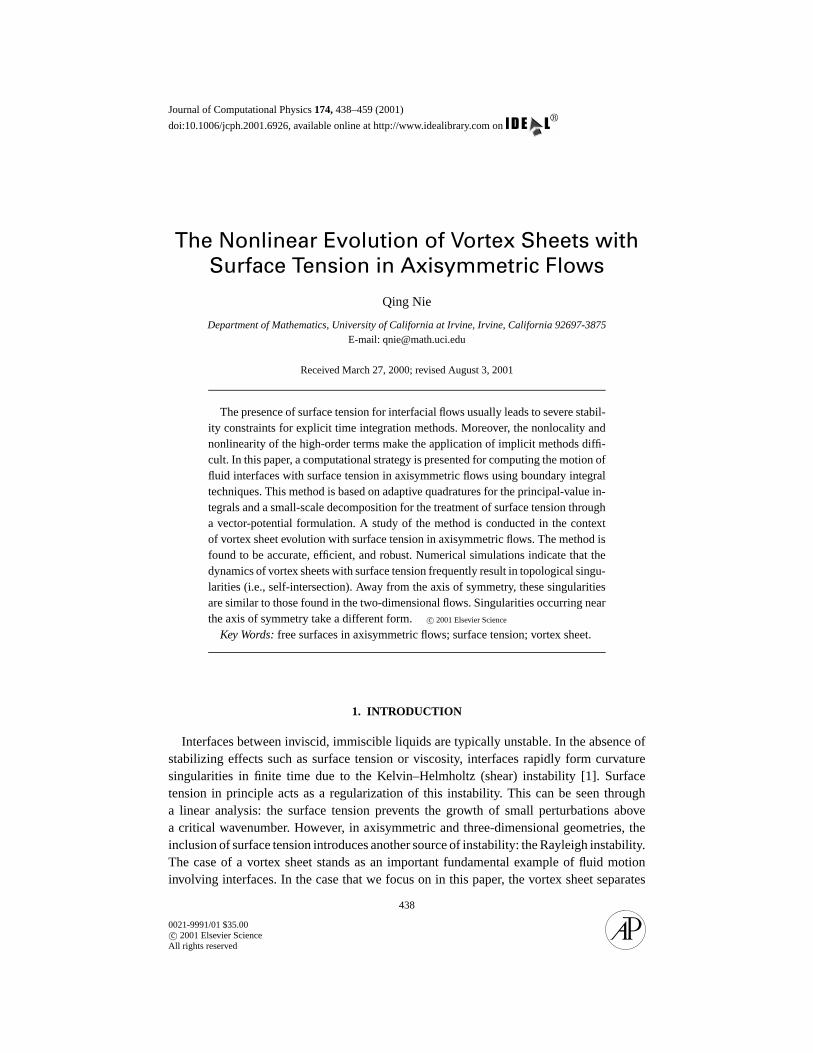
Journal of Computational Physics 174, 438–459 (2001)

doi:10.1006/jcph.2001.6926, available online at http://www.idealibrary.com on

The Nonlinear Evolution of Vortex Sheets with

Surface Tension in Axisymmetric Flows

Qing Nie

Department of Mathematics, University of California at Irvine, Irvine, California 92697-3875E-mail: [email protected]

Received March 27, 2000; revised August 3, 2001

The presence of surface tension for interfacial flows usually leads to severe stabil-ity constraints for explicit time integration methods. Moreover, the nonlocality andnonlinearity of the high-order terms make the application of implicit methods diffi-cult. In this paper, a computational strategy is presented for computing the motion offluid interfaces with surface tension in axisymmetric flows using boundary integraltechniques. This method is based on adaptive quadratures for the principal-value in-tegrals and a small-scale decomposition for the treatment of surface tension througha vector-potential formulation. A study of the method is conducted in the contextof vortex sheet evolution with surface tension in axisymmetric flows. The method isfound to be accurate, efficient, and robust. Numerical simulations indicate that thedynamics of vortex sheets with surface tension frequently result in topological singu-larities (i.e., self-intersection). Away from the axis of symmetry, these singularitiesare similar to those found in the two-dimensional flows. Singularities occurring nearthe axis of symmetry take a different form. c© 2001 Elsevier Science

Key Words: free surfaces in axisymmetric flows; surface tension; vortex sheet.

1. INTRODUCTION

Interfaces between inviscid, immiscible liquids are typically unstable. In the absence ofstabilizing effects such as surface tension or viscosity, interfaces rapidly form curvaturesingularities in finite time due to the Kelvin–Helmholtz (shear) instability [1]. Surfacetension in principle acts as a regularization of this instability. This can be seen througha linear analysis: the surface tension prevents the growth of small perturbations abovea critical wavenumber. However, in axisymmetric and three-dimensional geometries, theinclusion of surface tension introduces another source of instability: the Rayleigh instability.The case of a vortex sheet stands as an important fundamental example of fluid motioninvolving interfaces. In the case that we focus on in this paper, the vortex sheet separates

438

0021-9991/01 $35.00c© 2001 Elsevier Science

All rights reserved

VORTEX SHEETS IN AXISYMMETRIC FLOWS 439

two immiscible and density-matched fluids, and there is competition only between the shearinstability and the surface tension.

Boundary integral techniques provide a popular approach to computing the evolution ofinterfaces with surface tension. One of the major features of boundary integral techniquesis that the equations of motion may be reposed entirely along the interface, thus reducingthe complexity of the problem by one dimension. In addition, boundary integral techniquesare particularly convenient for the treatment of surface tension that requires the calculationof curvature [2–4].

For two-dimensional flows, surface tension has now been included in numerical studiesof many free-surface problems. These include the study of the rising gas bubble [5], vortexsheets with surface tension [6–11], the Rayleigh–Taylor instability [7, 8, 12, 13], and thegeneration of capillary waves [14]. See the recent review article by Hou et al. [4].

Until recently, it has been problematic to obtain stable numerical methods, even in twodimensions. In the context of the motion of vortex sheets with surface tension, Baker andNachbin [9] have demonstrated through linear analysis and nonlinear computations that themain cause of instability (the growth of the sawtooth mode) is the failure of the mesh torepresent vorticity created by the surface tension. They then developed a stable numericalmethod in which this instability is removed by using a midpoint rule to approximate theboundary integrals. Independently, Beale et al. [15, 16], and subsequently Ceniceros andHou [13] analyzed this numerical instability using a slightly different formulation andproposed alternative stable methods.

In addition, the presence of surface tension requires small time steps when an explicitmethod is used, and results in a strong stability constraint, 1t ≤ C(1s)3/2, where 1s isthe smallest arclength between two computational mesh points on the sheet. This is due tothe interface curvature that appears in the boundary condition for the vortex sheet strength.As an example, an explicit method based on Lagrangian motion accumulates the markersnear a stagnation point on the interface (reducing 1s as a result) and forces the use of anever-decreasing time step [7–9, 16].

In 1994, Hou et al. (HLS94) [10] introduced a new formulation and methods based ona small-scale decomposition of nonlinear equations. The main idea in this approach is toseparate the most singular part (e.g., the part with the highest derivative) of the equationfrom the rest and treat the singular part implicitly through a change of variable. In particular,the interface location is represented in terms of its local arclength s and its tangent angleθ . The most singular part of the normal velocity of the interface is found to be a Hilberttransformation of the vortex sheet strength, which can be diagonalized in Fourier space.As a result, it can be treated implicitly and efficiently along with the curvature θs . The newformulation has all the nice properties of time integration methods that are associated withhaving a linear highest-order term. The resulting methods do not have the severe stabilityconstraints usually associated with surface tension. This method has been successfully usedto study the long-time evolution of vortex sheets with surface tension [11].

In three dimensions, the study of vortex sheet motion has been restricted to the cases with-out surface tension. There is evidence for the formation of singularities in the axisymmetricgeometry [17–19] and for certain three-dimensional perturbations of a plane vortex sheet[20, 21]. In addition, by form-fitting the Fourier coefficients of the numerical solutions, it isfound that there exists curvature singularity and that singularity formations in axisymmet-ric and two-dimensional vortex sheets are very similar [18, 22, 23]. In this paper, we areinterested in simulations of vortex sheet motion with surface tension in axisymmetric flows.

440 QING NIE

Computing the motion of vortex sheets in axisymmetric flows using boundary integralmethods is more difficult than it is in two dimensions for several reasons. First, the principal-value integrals involve complete elliptic integrals and contain logarithmic singularities.Further, the integrand has large variation near the axis of symmetry [19, 24, 25] whenthe vortex sheets cross or approach the axis of symmetry. Consequently the design of anaccurate quadrature is difficult for axisymmetric flows. For example, the high-order method[26] designed for treating the logarithmic singularities in the integrand in 2-D loses itsaccuracy near the axis of symmetry and becomes a first-order method [19]. In 1998, Nieand Baker (NB98) [18] introduced a new quadrature technique for axisymmetric flows basedon a dipole representation of the vortex sheet through the vector-potential formulation. Inthis approach, high-order adaptive numerical quadratures are incorporated to ensure theaccurate calculation of the principal-value integrals by inserting more quadrature pointswhere the integrand has large variation.

The second major numerical difficulty is the strong time-step stability constraint thatarises due to the presence of surface tension. This is similar to the two-dimensional case.Until very recently, this stability constraint has been somewhat modified by regriddingthe interface markers at every time step or after several time steps and imposing surfacesmoothing in ad-hoc ways [27–29]. Experience shows that this does not entirely eliminatethe stability constraints and it only partially improves the computations.

In this study, we combine the small-scale decomposition technique presented for two-dimensional flows in HLS94 and the strategy using adaptive quadratures for axisymmetricflows in NB98 to develop accurate and efficient methods that can be used to study vortexsheets with surface tension in axisymmetric flows. We note that very recently Cenicerosand Si [30] developed a related algorithm that uses quadratures presented in [19] and thesmall-scale decomposition technique to study axisymmetric porous media flows. In [30]the effect of small surface tension on the dynamics of an axisymmetric flow is studied.

As shown in HLS94 the central reasons for using the small-scale decomposition techniqueare that the most singular terms in the equations can be identified, treated implicitly intemporal integration, and computed efficiently. Fortunately, we find this is achievable in theaxisymmetric case. In particular, the Lagrangian velocity of the vortex sheet is found to bedominated by a Hilbert transform of vortex sheet strength at small scales, similar to the two-dimensional case. For the surface tension term, the curvature in the axisymmetric geometryis a sum of curvatures in the meridian direction and in the azimuthal direction. At smallscales, this sum is dominated by its two-dimensional counterpart, the one from meridiandirection, because it contains the highest number of derivatives. In order to treat the termsimplicitly in the temporal scheme, we represent the vortex sheet in the meridian plane usingthe tangent angle θ and equal arclength L similar to the two-dimensional case (HLS94).The velocity for the vortex sheet is computed using a dipole representation through thevector-potential formulation (NB98). Adaptive quadratures are implemented for the sakeof efficiency and of accuracy for the calculations of principal-value integrals.

We use this method to calculate the evolution of an initially spherical vortex sheet andstudy the evolution of the vortex sheet for different values of surface tension and for differentchoices of the initial vortex sheet strength. The method is found to be robust and accurate.The computations show that the evolution of the vortex sheet sensitively depends on thesurface tension. In particular, for small surface tensions, the sheet develops a rolled-upstructure and the interface self-intersects (pinches off) away from the axis of symmetry.This type of pinch-off is found to be similar to the analogous pinch-off that occurs in


two-dimensional flows. For large surface tensions, the sheet necks down and the pinch-offoccurs at the axis of symmetry (r = 0). For this case we notice an overturning of the interface,which is not observed for the two-dimensional flows. For moderately sized surface tensions,the sheet evolves via a combination of spirals, necks, and pinch-offs.

The organization of the paper is as follows. In Section 2, we derive a formulation basedon the small-scale decomposition for axisymmetric flows. In Section 3, we describe thenumerical techniques and discuss the details of the implementation. In Section 4, we studythe accuracy of the numerical method and present the results. In Section 5, we present theconclusions and discussions.

2. FORMULATIONS

For an axisymmetric vortex sheet, we may represent the sheet position, denoted by 0, as

X = r(α, t)er + z(α, t)ez, (1)

using the cylindrical coordinates (r, z). The motion of 0 is given by

(rt , zt )= Vnn + T s, (2)

where n is the inward normal of the sheet with Vn as the inward normal velocity and s is thetangential direction of the sheet with T as a specified tangential velocity. We remark thatthe choice of T does not affect the motion of the sheet 0, and it only affects the definitionof α.

In the Lagrangian frame, the velocity of the sheet is given by the Biot–Savart integral[31]

ur =1

4πrP∫

γ ′(z′ − z)B0(α, α′)(F(k)+ B1(α, α

′)E(k)) dα′, (3)

uz =1

4πP∫

γ ′ B0(α, α′)(F(k)+ B2(α, α

′)E(k)) dα′, (4)

where F(k) and E(k) are the complete elliptic integrals of the first and second kind, re-spectively, with

k2 =4rr ′

(z − z′)2 + (r + r ′)2, B0(α, α

′) =2

((z − z′)2 + (r + r ′)2)1/2, (5)

B1(α, α′) = −

(z′ − z)2 + r ′2 + r2

(z − z′)2 + (r − r ′)2, B2(α, α

′) =r ′2 − r2 − (z′ − z)2

(z − z′)2 + (r − r ′)2, (6)

where r ′ = r(α′, t), etc. The vortex sheet strength γ (α, t) ≡ µα(α, t) can be determinedthrough the dipole sheet strength µ (NB98), which evolves via

∂µ

∂t= (T − s · u)µs − σκmean, (7)

442 QING NIE

where sα ≡√

r2α + z2

α and κmean ≡ κ + κ∞ is twice the mean curvature. Here κ and κ∞ arethe curvatures in the meridian and azimuthal directions, respectively:

κ =rαzαα − rααzα

s3α

κ∞ =zαrsα

. (8)

The normal velocity then is obtained from

Vn = u · n. (9)

The choice T = s · u corresponds to the Lagrangian frame.The motion of 0 can be reposed in terms of its local arclength derivatives sα and its

tangent angle θ defined implicitly from the definition of the tangent vector,

s(α, t)= (rα, zα)/sα = (cos θ(α, t), sin θ(α, t)). (10)

Then θ and sα satisfy

sαt = Tα − θαVn (11)

θt =Vnα + T θα

sα(12)

with T as yet unspecified.Because κ contains higher derivative of r and z than κ∞ in κmean, we obtain, after taking

a derivative of Eq. (7) with respect to α,

γt ∼ −σκα, (13)

where f ∼ g means that the difference between f and g is smoother than f and g. Thiscan be seen by an argument similar to that used for the small-scale decomposition in thetwo-dimensional case (HLS94).

Next we examine the leading-order behavior for Vn . From the Biot–Savart integrals for(ur , uz), with n = (−zs, rs), we obtain

Vn = (ur , uz) · (−zs, rs)∼ −1

2πsαP∫

γ ′

α − α′dα′ as α → α′. (14)

Here, we have used the fact that for r ≡ r(α) 6= 0 the leading order terms of the integrandsin (3) and (4) are

−2rγ ′zα

s2α(α

′ − α)and

2γ ′rαs2α(α

′ − α), (15)

respectively.Consequently, we regroup Vn as

Vn = −1

2sαH(γ )+ remainder, (16)


where H is the Hilbert transform and the remaining term is smoother than the Hilberttransform.

Using the fact that θs = κ , we obtain the small-scale decomposition equation for theaxisymmetric vortex sheet,

θt = −1

2

1

sα

(

1

sαH(γ )

)

α

+ P (17)

γt = −σ

(

θα

sα

)

α

+ Q, (18)

where

P ≡1

2

1

sα

(

1

sαH(γ )

)

α

+Vnα + T θα

sα(19)

Q ≡ ((T − s · u)µs − σκ∞)α. (20)

The form of the equations is exactly the same as in the two-dimensional case except thatP and Q are different. In the two-dimensional case, P and Q involve only Birkhoff–Rottintegrals while for the axisymmetric case κ∞ is present in Q. Moreover, Vn and u are moredifficult to compute.

3. NUMERICAL METHODS

Following HLS94, we use a semiimplicit temporal scheme for Eq. (17) and (18). To avoidsolving a linear system during the time integration, we require sα to be a function of time only,

sα(α, t)=L(t)

2π≡ 1/M(t). (21)

This can be achieved by choosing the special tangential velocity

T (α, t)=α

2π

∫ 2π

0θα′ Vn dα′ −

∫ α

0θα′ Vn dα′. (22)

Consequently, Eq. (11) for sα becomes

L t =

∫ 2π

0θα′ Vn dα′. (23)

Denote f (k) to be the Fourier coefficient of f . By applying the Crank–Nicholson dis-cretization to the leading-order term in the Fourier space in Eq. (17) and (18), we obtainthe following diagonalized system in Fourier space:

θ (k)n+1 − θ (k)n−1

21t= −

|k|

4((Mn+1)2γ (k)n+1 + (Mn−1)2γ (k)n−1)+ Pn(k) (24)

γ (k)n+1 − γ (k)n−1

21t= σ

k2

2(Mn+1θ (k)n+1 + Mn−1θ (k)n−1)+ Qn(k). (25)

The quantities θn+1(k) and γ n+1(k) can be calculated explicitly by inverting a 2 × 2 matrix.

444 QING NIE

L should be updated by an explicit method such as the second-order Adams–Bashforthdiscretization of Eq. (23). The computations of θ and γ will require this updated L . OnceL and θ are known, we can numerically integrate Eq. (10) to obtain (r, z). Similarly, we cancalculate µ through the numerical integration of γ .

The above formulation is the same as in HLS94 except that Vn, P , and Q are different.For P and Q, the essential parts involve Vn and u. As studied in NB98, one of the majorchallenges of using the boundary integral technique to compute free surfaces in an axisym-metric flow is the accurate evaluations of the velocity integrals. This is particularly true forthe motion of vortex sheets with small surface tensions σ because for σ = 0 the govern-ing equation is ill-posed. In NB98, we developed a very efficient and accurate strategy tocompute Vn and u based on a vector-potential formulation with an adaptive quadrature. Weimplement the same method for σ 6= 0 in this paper. Below, we present a brief sketch ofthis technique.

The normal velocity is computed through a vector potential by

Vn =ψα

r(26)

and (3) and (4) can be rewritten as

ur =

(

φαrα −ψα

rzα

)

1

s2α

, (27)

uz =

(

φαzα +ψα

rrα

)

1

s2α

, (28)

where the potential function φ and the vector potential function ψ have the followingintegral representations,

φ(α) =1

4πP∫

(µ′ −µ)B0(α, α′)(z′

αF(k)+ C1(α, α′)E(k)) dα′ +

1

2µ, (29)

ψ(α) =1

4πP∫

(µ′ −µ)B0(α, α′)([r ′

αr ′ − z′α(z − z′)]F(k)+ C2(α, α

′)E(k)) dα′, (30)

with

C1(α, α′) = −

(z − z′)[z′α(z − z′)− 2r ′r ′

α] + (r2 − r ′2)z′α

(z − z′)2 + (r − r ′)2(31)

and

C2(α, α′)=

(z − z′)([z′α(z − z′)− r ′

αr ′](z − z′)+ z′α(r

2 + r ′2))+ (r2 − r ′2)r ′αr ′

(z − z′)2 + (r − r ′)2. (32)

The integrands in (29) and (30) exhibit the following asymptotic behavior,

−zαµα

r(α′ − α) ln |α − α′| and −2µαr, (33)

respectively, compared with the pole singularities 1/(α′ − α) for the integrands in (3) and(4). This property of the integrands allows one to use more sophisticated quadratures to


compute the integrals and improve the accuracy. In particular, the difficulty arising fromlarge variations of the integrand near the axis, r = 0, which in turn causes large loss ofresolution, can be overcome by inserting more quadrature points around r = 0.

One special class of quadratures we employed in NB98 was the Gauss–Kronrod quadra-ture [32, 33]. The major difference between this quadrature and standard ones is its progres-sive nature for the construction of the quadrature; i.e., one rule can be generated by addingnew points to another Gaussian rule. This progressive property is crucial for any adaptivestrategies. In this study, we use a 7- to 15-point, Gauss–Kronrod quadrature. We bisect theintegration intervals and estimate the error of the numerical integration over each intervalby measuring the difference between the 7-point Gauss quadrature and 15-point Kronrodrule. A globally adaptive strategy is to bisect the interval with the largest error estimate untilthe error is less than a prescribed tolerance. We used the freely available software packageQuadpack [34] to implement this strategy. The recursive formulae [35, p. 297] are used forthe evaluation of both F(k) and E(k).

Another strategy, which exploits the logarithmic behavior of the integrands in (29) and(30), is also implemented using Clenshaw–Curtis quadrature [36, 37]. This method is basedon an expansion of the integrand in a series of Chebyshev polynomials. The method variesthe number of terms in the series to reach a specified level of accuracy, and thus is naturallyadaptive.

We approximate the closed surface by a set of boundary nodes along the contour in the(r, z) meridional plane, (ri , zi ) ≡ (r(αi ), z(αi )) for i = 1, . . . , N , where αi = iπ/(N − 1).We calculate φ and ψ at those points, denoted by φi and ψi . Although the integrands in(29) and (30) are continuous when α=α′, their derivatives are not. So we split the integrals(29) and (30) into two parts: one integrated from 0 to αi , another one from αi to π , with thefollowing form:

∫ π

0f (α, α′) dα′ +

∫ α

0g1(α, α

′) ln(α − α′) dα′ +

∫ π

α

g2(α, α′) ln(α′ − α) dα′. (34)

Next, we employ the Gauss–Kronrod rule on the first integral in (34), and modifiedClenshaw–Curtis rule on the second and third integrals in (34). For (r, z) that are not atthe collocation point αi during the integral evaluations, we approximate them throughinterpolation using a quintic spline [38]. Consequently, the order of the accuracy for thismethod is O(N−6).

Once φi and ψi are evaluated, their derivatives are obtained using fast Fourier transfor-mation (FFT). Derivatives such as zα, rα are also calculated using FFT. The evaluation ofψα/r at r = 0 is treated separately by computing ψαα/rα .

It has been found that for two-dimensional free-surface flows with surface tension [9, 16],using splines for numerical derivatives introduces numerical instability. However, this nume-rical instability can be suppressed by filtering [16]. In all computations presented, we employa similar spectral Fourier filter,

e−c0(|k|/N )pf (k), (35)

with a cutoff filter [39] which sets all Fourier coefficients below a filter level ε f to zero.We typically chose c0 = 10, p = 15, and ε f = 10−12 unless otherwise specified. This filteris implemented at every time step for z, r , and γ ; i.e., each Fourier coefficient of z, r , andγ is replaced by Eq. (35) and furthermore, all coefficients below ε f are set to zero.

446 QING NIE

4. NUMERICAL RESULTS

We follow previous work [17, 40] using a sphere as the initial shape of vortex sheetthroughout this paper. The parameterization of the sphere surface is

r(α, 0)= sin(α) z(α, 0)= −cos(α) α ∈ [0, π ]. (36)

We first consider

µ(α, 0) = −cos(α) α ∈ [0, π ] (37)

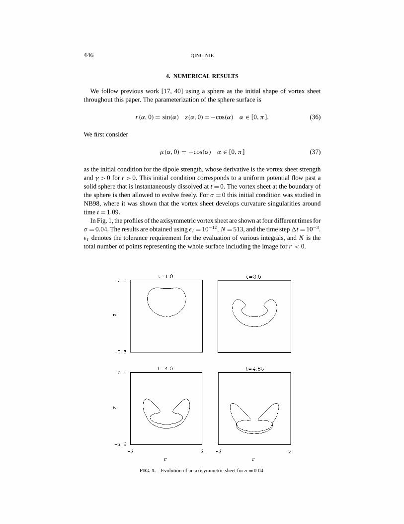
as the initial condition for the dipole strength, whose derivative is the vortex sheet strengthand γ > 0 for r > 0. This initial condition corresponds to a uniform potential flow past asolid sphere that is instantaneously dissolved at t = 0. The vortex sheet at the boundary ofthe sphere is then allowed to evolve freely. For σ = 0 this initial condition was studied inNB98, where it was shown that the vortex sheet develops curvature singularities aroundtime t = 1.09.

In Fig. 1, the profiles of the axisymmetric vortex sheet are shown at four different times forσ = 0.04. The results are obtained using εI = 10−12, N = 513, and the time step1t = 10−3.εI denotes the tolerance requirement for the evaluation of various integrals, and N is thetotal number of points representing the whole surface including the image for r < 0.

FIG. 1. Evolution of an axisymmetric sheet for σ = 0.04.


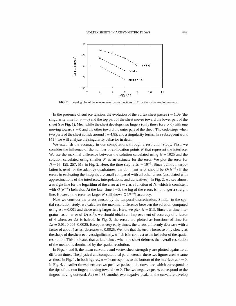
FIG. 2. Log–log plot of the maximum errors as functions of N for the spatial resolution study.

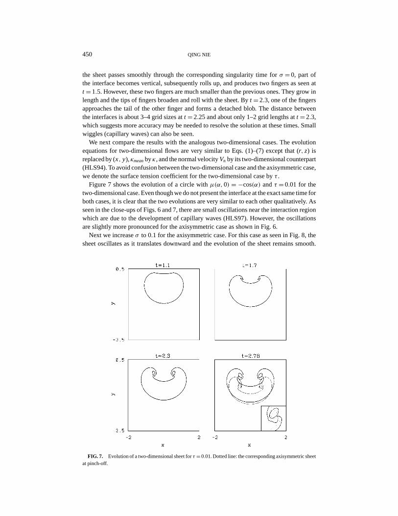
In the presence of surface tension, the evolution of the vortex sheet passes t = 1.09 (thesingularity time for σ = 0) and the top part of the sheet moves toward the lower part of thesheet (see Fig. 1). Meanwhile the sheet develops two fingers (only those for r > 0) with onemoving toward r = 0 and the other toward the outer part of the sheet. The code stops whentwo parts of the sheet collide around t = 4.85, and a singularity forms. In a subsequent work[41], we will analyze the singularity behavior in detail.

We establish the accuracy in our computations through a resolution study. First, weconsider the influence of the number of collocation points N that represent the interface.We use the maximal difference between the solution calculated using N = 1025 and thesolution calculated using smaller N as an estimate for the error. We plot the error forN = 65, 129, 257, 513 in Fig. 2. Here, the time step is 1t = 10−3. Since quintic interpo-lation is used for the adaptive quadratures, the dominant error should be O(N−6) if theerrors in evaluating the integrals are small compared with all other errors (associated withapproximations of the interfaces, interpolations, and derivatives). In Fig. 2, we see almosta straight line for the logarithm of the error at t = 2 as a function of N , which is consistentwith O(N−6) behavior. At the later time t = 3, the log of the errors is no longer a straightline. However, the error for larger N still shows O(N−6) accuracy.

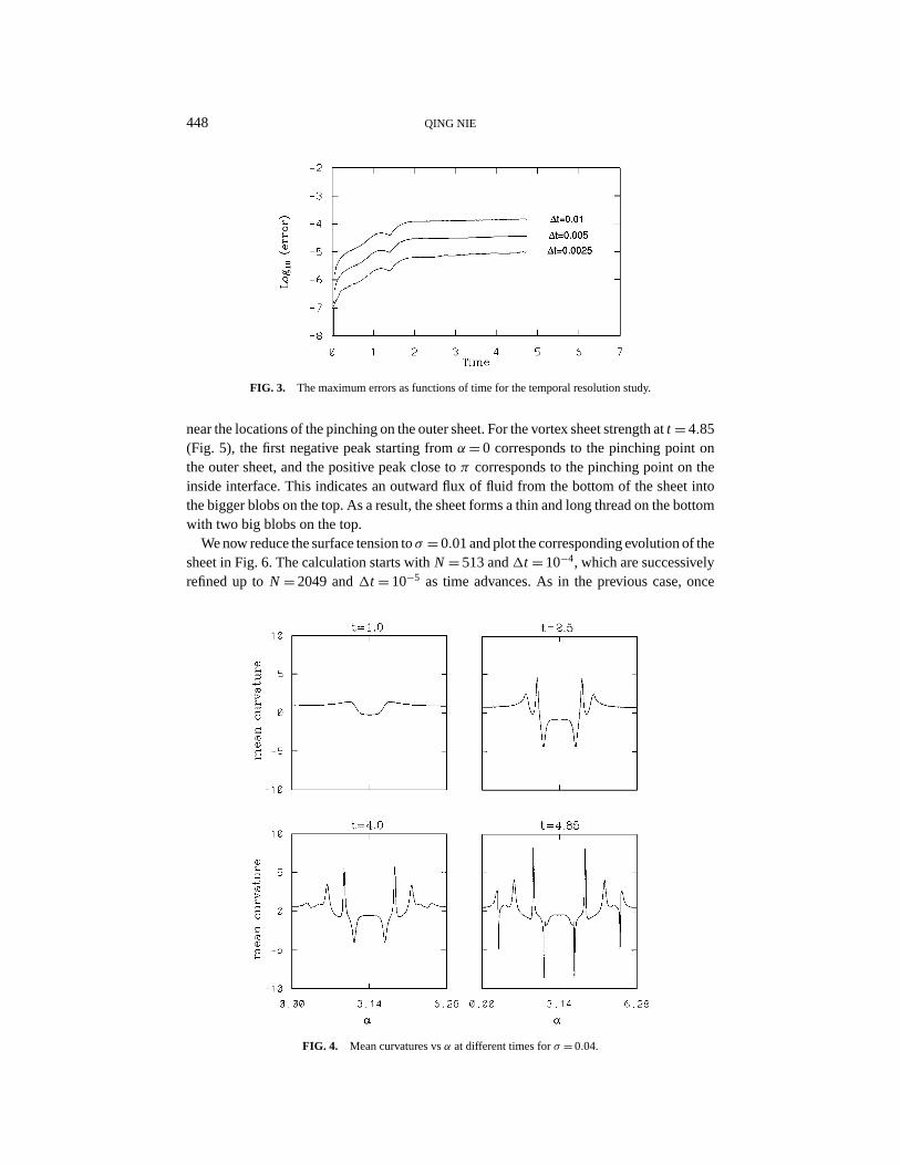
Next we consider the errors caused by the temporal discretization. Similar to the spa-tial resolution study, we calculate the maximal difference between the solution computedusing 1t = 0.001 and those using larger 1t . Here, we pick N = 513. Since our time inte-grator has an error of O(1t2), we should obtain an improvement of accuracy of a factorof 4 whenever 1t is halved. In Fig. 3, the errors are plotted as functions of time for1t = 0.01, 0.005, 0.0025. Except at very early times, the errors uniformly decrease with afactor of about 4 as1t decreases to 0.0025. We note that the errors increase only slowly asthe shape of the sheet evolves significantly, which is in contrast to the behavior of the spatialresolution. This indicates that at later times when the sheet deforms the overall resolutionof the method is dominated by the spatial resolution.

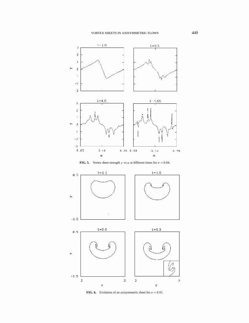
In Figs. 4 and 5, the mean curvature and vortex sheet strength γ are plotted against α atdifferent times. The physical and computational parameters in these two figures are the sameas those in Fig. 1. In both figures, α= 0 corresponds to the bottom of the interface at r = 0.In Fig. 4, at earlier times there are two positive peaks of the curvature, which correspond tothe tips of the two fingers moving toward r = 0. The two negative peaks correspond to thefingers moving outward. At t = 4.85, another two negative peaks in the curvature develop

448 QING NIE

FIG. 3. The maximum errors as functions of time for the temporal resolution study.

near the locations of the pinching on the outer sheet. For the vortex sheet strength at t = 4.85(Fig. 5), the first negative peak starting from α= 0 corresponds to the pinching point onthe outer sheet, and the positive peak close to π corresponds to the pinching point on theinside interface. This indicates an outward flux of fluid from the bottom of the sheet intothe bigger blobs on the top. As a result, the sheet forms a thin and long thread on the bottomwith two big blobs on the top.

We now reduce the surface tension to σ = 0.01 and plot the corresponding evolution of thesheet in Fig. 6. The calculation starts with N = 513 and1t = 10−4, which are successivelyrefined up to N = 2049 and 1t = 10−5 as time advances. As in the previous case, once

FIG. 4. Mean curvatures vs α at different times for σ = 0.04.


FIG. 5. Vortex sheet strength γ vs α at different times for σ = 0.04.


450 QING NIE

the sheet passes smoothly through the corresponding singularity time for σ = 0, part ofthe interface becomes vertical, subsequently rolls up, and produces two fingers as seen att = 1.5. However, these two fingers are much smaller than the previous ones. They grow inlength and the tips of fingers broaden and roll with the sheet. By t = 2.3, one of the fingersapproaches the tail of the other finger and forms a detached blob. The distance betweenthe interfaces is about 3–4 grid sizes at t = 2.25 and about only 1–2 grid lengths at t = 2.3,which suggests more accuracy may be needed to resolve the solution at these times. Smallwiggles (capillary waves) can also be seen.

We next compare the results with the analogous two-dimensional cases. The evolutionequations for two-dimensional flows are very similar to Eqs. (1)–(7) except that (r, z) isreplaced by (x, y), κmean by κ , and the normal velocity Vn by its two-dimensional counterpart(HLS94). To avoid confusion between the two-dimensional case and the axisymmetric case,we denote the surface tension coefficient for the two-dimensional case by τ .

Figure 7 shows the evolution of a circle with µ(α, 0) = −cos(α) and τ = 0.01 for thetwo-dimensional case. Even though we do not present the interface at the exact same time forboth cases, it is clear that the two evolutions are very similar to each other qualitatively. Asseen in the close-ups of Figs. 6 and 7, there are small oscillations near the interaction regionwhich are due to the development of capillary waves (HLS97). However, the oscillationsare slightly more pronounced for the axisymmetric case as shown in Fig. 6.

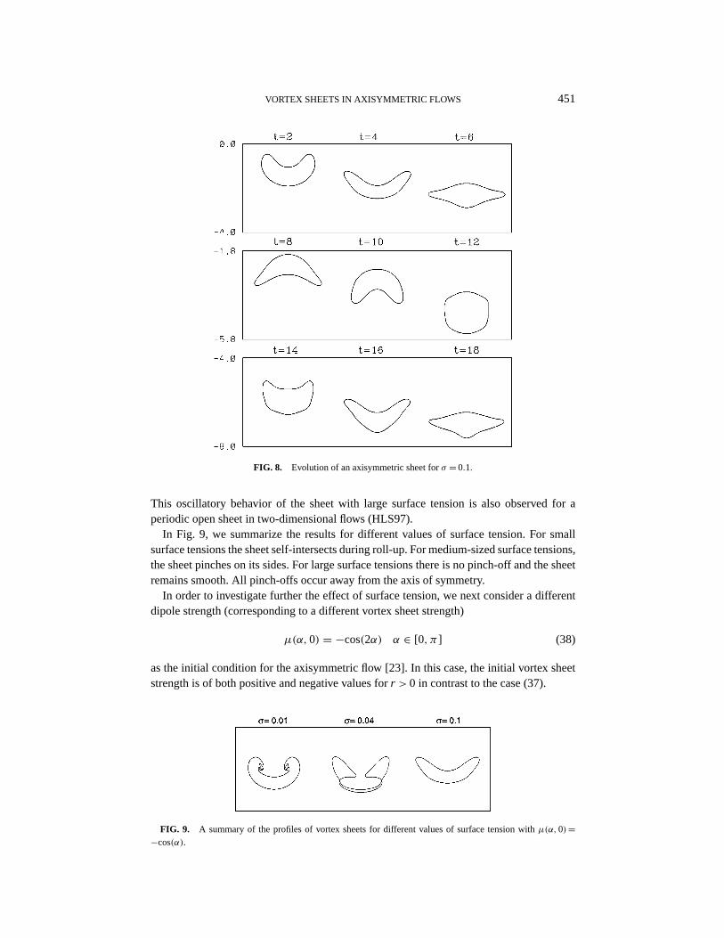
Next we increase σ to 0.1 for the axisymmetric case. For this case as seen in Fig. 8, thesheet oscillates as it translates downward and the evolution of the sheet remains smooth.

FIG. 7. Evolution of a two-dimensional sheet for τ = 0.01. Dotted line: the corresponding axisymmetric sheetat pinch-off.



This oscillatory behavior of the sheet with large surface tension is also observed for aperiodic open sheet in two-dimensional flows (HLS97).

In Fig. 9, we summarize the results for different values of surface tension. For smallsurface tensions the sheet self-intersects during roll-up. For medium-sized surface tensions,the sheet pinches on its sides. For large surface tensions there is no pinch-off and the sheetremains smooth. All pinch-offs occur away from the axis of symmetry.

In order to investigate further the effect of surface tension, we next consider a differentdipole strength (corresponding to a different vortex sheet strength)

µ(α, 0) = −cos(2α) α ∈ [0, π ] (38)

as the initial condition for the axisymmetric flow [23]. In this case, the initial vortex sheetstrength is of both positive and negative values for r > 0 in contrast to the case (37).

FIG. 9. A summary of the profiles of vortex sheets for different values of surface tension with µ(α, 0)=−cos(α).

452 QING NIE

FIG. 10. Evolution of an axisymmetric sheet for σ = 0.2 and µ(α, 0)= −cos(2α).

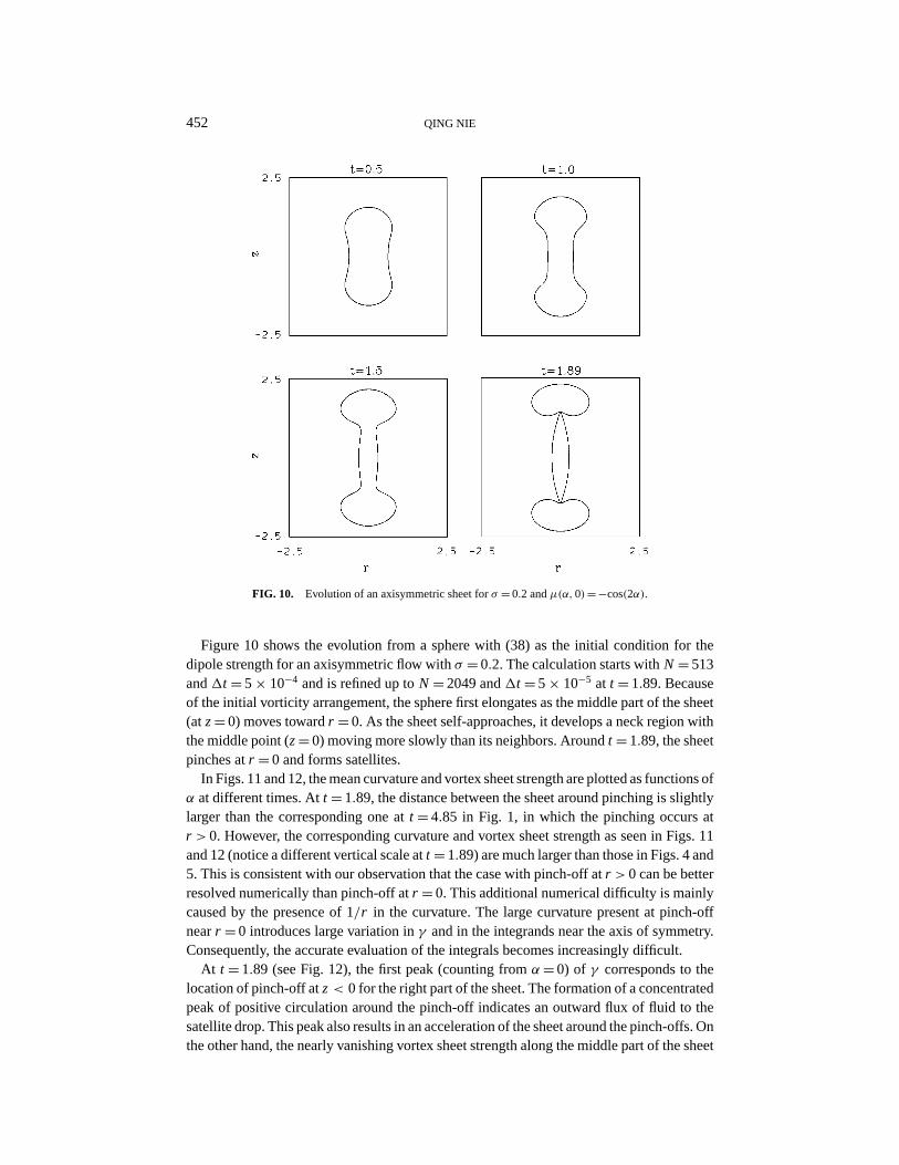
Figure 10 shows the evolution from a sphere with (38) as the initial condition for thedipole strength for an axisymmetric flow with σ = 0.2. The calculation starts with N = 513and 1t = 5 × 10−4 and is refined up to N = 2049 and 1t = 5 × 10−5 at t = 1.89. Becauseof the initial vorticity arrangement, the sphere first elongates as the middle part of the sheet(at z = 0) moves toward r = 0. As the sheet self-approaches, it develops a neck region withthe middle point (z = 0) moving more slowly than its neighbors. Around t = 1.89, the sheetpinches at r = 0 and forms satellites.

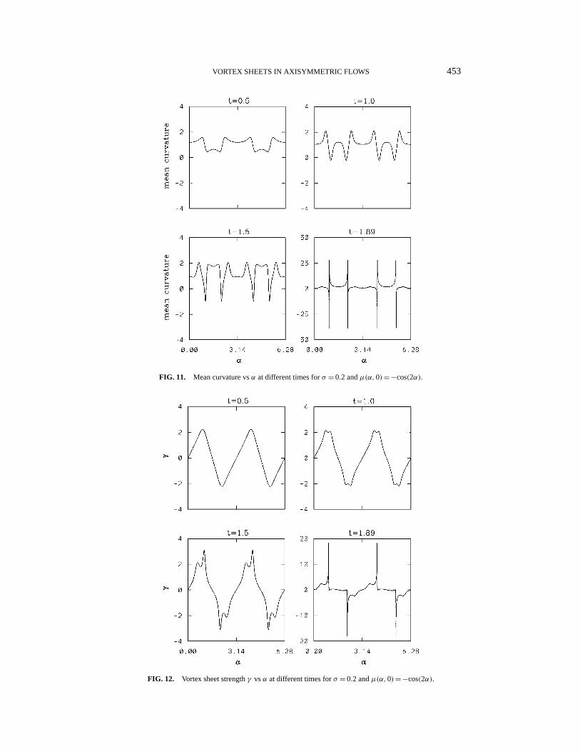
In Figs. 11 and 12, the mean curvature and vortex sheet strength are plotted as functions ofα at different times. At t = 1.89, the distance between the sheet around pinching is slightlylarger than the corresponding one at t = 4.85 in Fig. 1, in which the pinching occurs atr > 0. However, the corresponding curvature and vortex sheet strength as seen in Figs. 11and 12 (notice a different vertical scale at t = 1.89) are much larger than those in Figs. 4 and5. This is consistent with our observation that the case with pinch-off at r > 0 can be betterresolved numerically than pinch-off at r = 0. This additional numerical difficulty is mainlycaused by the presence of 1/r in the curvature. The large curvature present at pinch-offnear r = 0 introduces large variation in γ and in the integrands near the axis of symmetry.Consequently, the accurate evaluation of the integrals becomes increasingly difficult.

At t = 1.89 (see Fig. 12), the first peak (counting from α= 0) of γ corresponds to thelocation of pinch-off at z < 0 for the right part of the sheet. The formation of a concentratedpeak of positive circulation around the pinch-off indicates an outward flux of fluid to thesatellite drop. This peak also results in an acceleration of the sheet around the pinch-offs. Onthe other hand, the nearly vanishing vortex sheet strength along the middle part of the sheet


FIG. 11. Mean curvature vs α at different times for σ = 0.2 and µ(α, 0)= −cos(2α).

FIG. 12. Vortex sheet strength γ vs α at different times for σ = 0.2 and µ(α, 0)= −cos(2α).

454 QING NIE

FIG. 13. Evolution of a two-dimensional sheet for τ = 0.2 and µ(α, 0)= −cos(2α). Dotted line: the corre-sponding axisymmetric sheet at pinch-off.

(the part between the two peaks with opposite signs) is responsible for its slower motion.As a result the sheet around the pinching region accelerates to r = 0 with the middle partof the sheet left behind, and the formation of a satellite drop becomes inevitable.

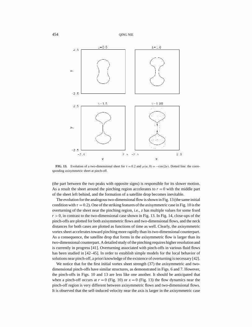
The evolution for the analogous two-dimensional flow is shown in Fig. 13 (the same initialcondition with τ = 0.2). One of the striking features of the axisymmetric case in Fig. 10 is theoverturning of the sheet near the pinching region, i.e., z has multiple values for some fixedr > 0, in contrast to the two-dimensional case shown in Fig. 13. In Fig. 14, close-ups of thepinch-offs are plotted for both axisymmetric flows and two-dimensional flows, and the neckdistances for both cases are plotted as functions of time as well. Clearly, the axisymmetricvortex sheet accelerates toward pinching more rapidly than its two-dimensional counterpart.As a consequence, the satellite drop that forms in the axisymmetric flow is larger than itstwo-dimensional counterpart. A detailed study of the pinching requires higher resolution andis currently in progress [41]. Overturning associated with pinch-offs in various fluid flowshas been studied in [42–45]. In order to establish simple models for the local behavior ofsolutions near pinch-off, a priori knowledge of the existence of overturning is necessary [42].

We notice that for the first initial vortex sheet strength (37) the axisymmetric and two-dimensional pinch-offs have similar structures, as demonstrated in Figs. 6 and 7. However,the pinch-offs in Figs. 10 and 13 are less like one another. It should be anticipated thatwhen a pinch-off occurs at r = 0 (Fig. 10) or x = 0 (Fig. 13) the flow dynamics near thepinch-off region is very different between axisymmetric flows and two-dimensional flows.It is observed that the self-induced velocity near the axis is larger in the axisymmetric case

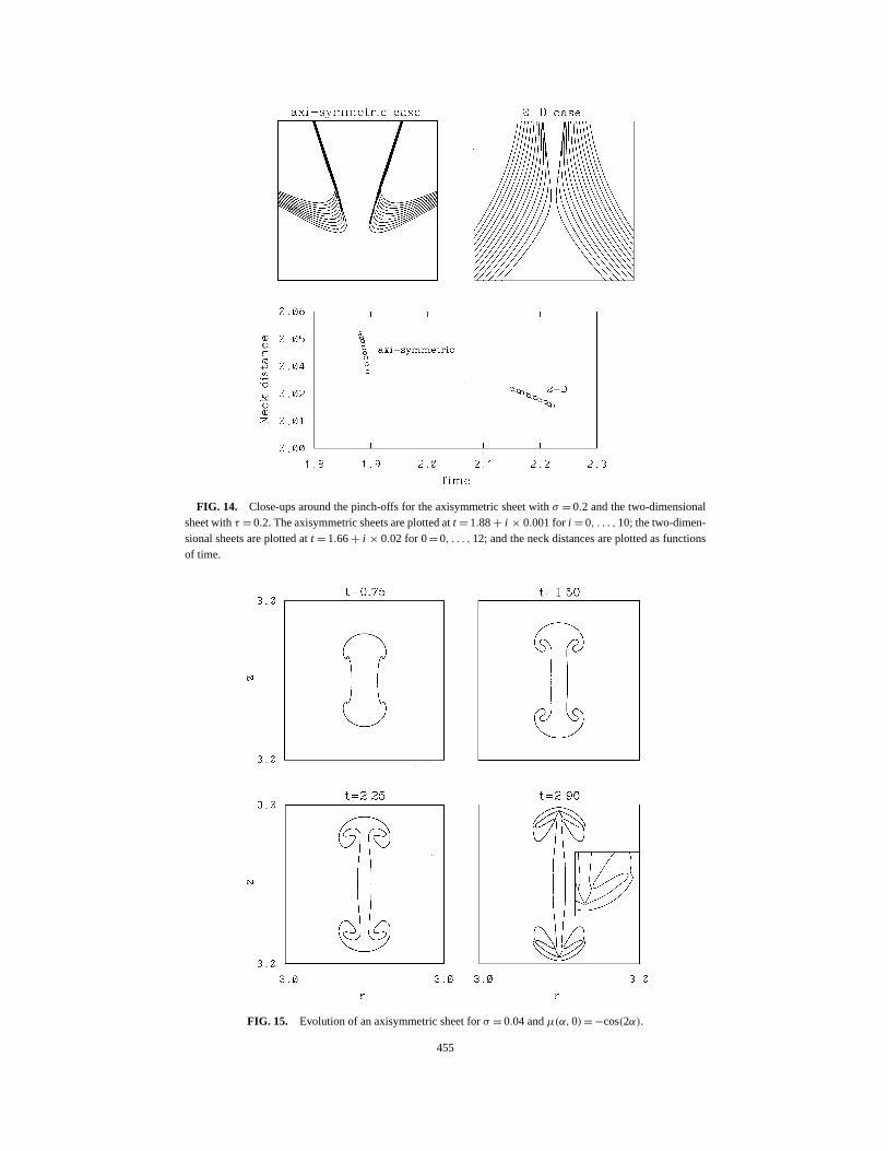
FIG. 14. Close-ups around the pinch-offs for the axisymmetric sheet with σ = 0.2 and the two-dimensionalsheet with τ = 0.2. The axisymmetric sheets are plotted at t = 1.88 + i × 0.001 for i = 0, . . . , 10; the two-dimen-sional sheets are plotted at t = 1.66 + i × 0.02 for 0 = 0, . . . , 12; and the neck distances are plotted as functionsof time.


455

456 QING NIE


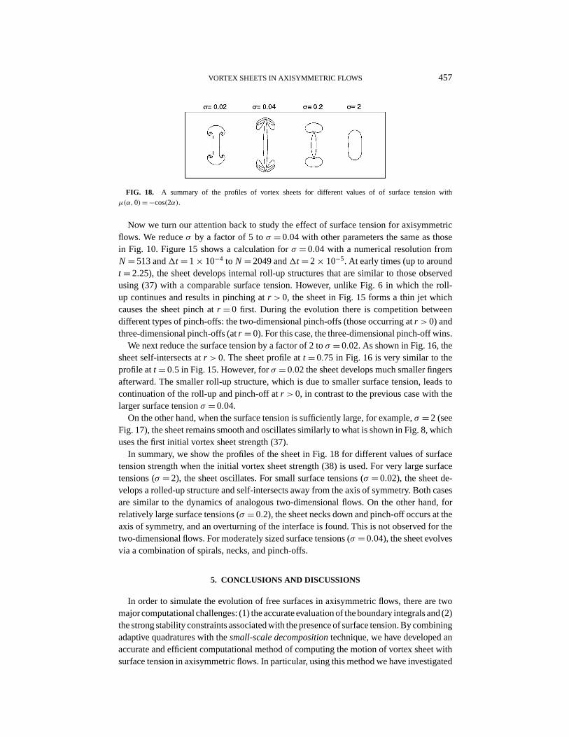
than in the two-dimensional case, and as a result, stronger local jets develop and acceleratethe pinch-off. Consequently there is overturning in the axisymmetric case and not in thetwo-dimensional case. The reason for the larger self-induced velocity in the axisymmetriccase is likely due to the filament curvature, which is large near the axis. Away from theaxis, the axisymmetric curvature is closer to the planar one and as a result, the self-inducedvelocities as well as the shapes of the pinch-offs are more comparable.

FIG. 17. Evolution of an axisymmetric sheet for σ = 2 and µ(α, 0)= −cos(2α).


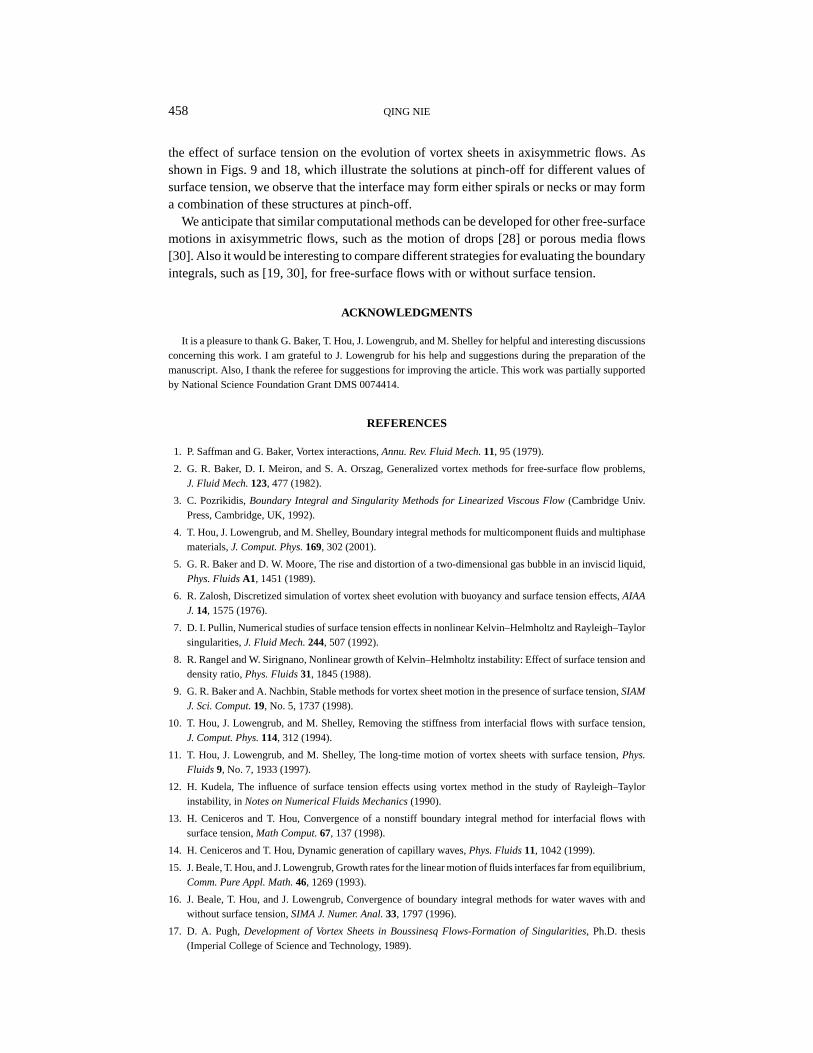
FIG. 18. A summary of the profiles of vortex sheets for different values of of surface tension withµ(α, 0)= −cos(2α).

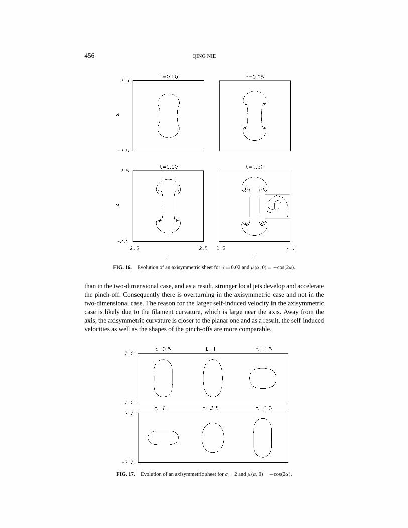
Now we turn our attention back to study the effect of surface tension for axisymmetricflows. We reduce σ by a factor of 5 to σ = 0.04 with other parameters the same as thosein Fig. 10. Figure 15 shows a calculation for σ = 0.04 with a numerical resolution fromN = 513 and1t = 1 × 10−4 to N = 2049 and1t = 2 × 10−5. At early times (up to aroundt = 2.25), the sheet develops internal roll-up structures that are similar to those observedusing (37) with a comparable surface tension. However, unlike Fig. 6 in which the roll-up continues and results in pinching at r > 0, the sheet in Fig. 15 forms a thin jet whichcauses the sheet pinch at r = 0 first. During the evolution there is competition betweendifferent types of pinch-offs: the two-dimensional pinch-offs (those occurring at r > 0) andthree-dimensional pinch-offs (at r = 0). For this case, the three-dimensional pinch-off wins.

We next reduce the surface tension by a factor of 2 to σ = 0.02. As shown in Fig. 16, thesheet self-intersects at r > 0. The sheet profile at t = 0.75 in Fig. 16 is very similar to theprofile at t = 0.5 in Fig. 15. However, for σ = 0.02 the sheet develops much smaller fingersafterward. The smaller roll-up structure, which is due to smaller surface tension, leads tocontinuation of the roll-up and pinch-off at r > 0, in contrast to the previous case with thelarger surface tension σ = 0.04.

On the other hand, when the surface tension is sufficiently large, for example, σ = 2 (seeFig. 17), the sheet remains smooth and oscillates similarly to what is shown in Fig. 8, whichuses the first initial vortex sheet strength (37).

In summary, we show the profiles of the sheet in Fig. 18 for different values of surfacetension strength when the initial vortex sheet strength (38) is used. For very large surfacetensions (σ = 2), the sheet oscillates. For small surface tensions (σ = 0.02), the sheet de-velops a rolled-up structure and self-intersects away from the axis of symmetry. Both casesare similar to the dynamics of analogous two-dimensional flows. On the other hand, forrelatively large surface tensions (σ = 0.2), the sheet necks down and pinch-off occurs at theaxis of symmetry, and an overturning of the interface is found. This is not observed for thetwo-dimensional flows. For moderately sized surface tensions (σ = 0.04), the sheet evolvesvia a combination of spirals, necks, and pinch-offs.

5. CONCLUSIONS AND DISCUSSIONS

In order to simulate the evolution of free surfaces in axisymmetric flows, there are twomajor computational challenges: (1) the accurate evaluation of the boundary integrals and (2)the strong stability constraints associated with the presence of surface tension. By combiningadaptive quadratures with the small-scale decomposition technique, we have developed anaccurate and efficient computational method of computing the motion of vortex sheet withsurface tension in axisymmetric flows. In particular, using this method we have investigated

458 QING NIE

the effect of surface tension on the evolution of vortex sheets in axisymmetric flows. Asshown in Figs. 9 and 18, which illustrate the solutions at pinch-off for different values ofsurface tension, we observe that the interface may form either spirals or necks or may forma combination of these structures at pinch-off.

We anticipate that similar computational methods can be developed for other free-surfacemotions in axisymmetric flows, such as the motion of drops [28] or porous media flows[30]. Also it would be interesting to compare different strategies for evaluating the boundaryintegrals, such as [19, 30], for free-surface flows with or without surface tension.

ACKNOWLEDGMENTS

It is a pleasure to thank G. Baker, T. Hou, J. Lowengrub, and M. Shelley for helpful and interesting discussionsconcerning this work. I am grateful to J. Lowengrub for his help and suggestions during the preparation of themanuscript. Also, I thank the referee for suggestions for improving the article. This work was partially supportedby National Science Foundation Grant DMS 0074414.

REFERENCES

1. P. Saffman and G. Baker, Vortex interactions, Annu. Rev. Fluid Mech. 11, 95 (1979).

2. G. R. Baker, D. I. Meiron, and S. A. Orszag, Generalized vortex methods for free-surface flow problems,J. Fluid Mech. 123, 477 (1982).

3. C. Pozrikidis, Boundary Integral and Singularity Methods for Linearized Viscous Flow (Cambridge Univ.Press, Cambridge, UK, 1992).

4. T. Hou, J. Lowengrub, and M. Shelley, Boundary integral methods for multicomponent fluids and multiphasematerials, J. Comput. Phys. 169, 302 (2001).

5. G. R. Baker and D. W. Moore, The rise and distortion of a two-dimensional gas bubble in an inviscid liquid,Phys. Fluids A1, 1451 (1989).

6. R. Zalosh, Discretized simulation of vortex sheet evolution with buoyancy and surface tension effects, AIAAJ. 14, 1575 (1976).

7. D. I. Pullin, Numerical studies of surface tension effects in nonlinear Kelvin–Helmholtz and Rayleigh–Taylorsingularities, J. Fluid Mech. 244, 507 (1992).

8. R. Rangel and W. Sirignano, Nonlinear growth of Kelvin–Helmholtz instability: Effect of surface tension anddensity ratio, Phys. Fluids 31, 1845 (1988).

9. G. R. Baker and A. Nachbin, Stable methods for vortex sheet motion in the presence of surface tension, SIAMJ. Sci. Comput. 19, No. 5, 1737 (1998).

10. T. Hou, J. Lowengrub, and M. Shelley, Removing the stiffness from interfacial flows with surface tension,J. Comput. Phys. 114, 312 (1994).

11. T. Hou, J. Lowengrub, and M. Shelley, The long-time motion of vortex sheets with surface tension, Phys.Fluids 9, No. 7, 1933 (1997).

12. H. Kudela, The influence of surface tension effects using vortex method in the study of Rayleigh–Taylorinstability, in Notes on Numerical Fluids Mechanics (1990).

13. H. Ceniceros and T. Hou, Convergence of a nonstiff boundary integral method for interfacial flows withsurface tension, Math Comput. 67, 137 (1998).

14. H. Ceniceros and T. Hou, Dynamic generation of capillary waves, Phys. Fluids 11, 1042 (1999).

15. J. Beale, T. Hou, and J. Lowengrub, Growth rates for the linear motion of fluids interfaces far from equilibrium,Comm. Pure Appl. Math. 46, 1269 (1993).

16. J. Beale, T. Hou, and J. Lowengrub, Convergence of boundary integral methods for water waves with andwithout surface tension, SIMA J. Numer. Anal. 33, 1797 (1996).

17. D. A. Pugh, Development of Vortex Sheets in Boussinesq Flows-Formation of Singularities, Ph.D. thesis(Imperial College of Science and Technology, 1989).


18. Q. Nie and G. R. Baker, Application of adaptive quadrature to axi-symmetric vortex sheet motion, J. Comput.Phys. 143, 49 (1998).

19. M. Nitsche, Axi-symmetric vortex sheet motion: Accurate evaluation of the principal value integral, SIAM J.Sci. Comput. 21, No. 3, 1066 (1999).

20. T. Ishihara and Y. Kaneda, Singularity formation in three-dimensional motion of a vortex sheet, J. FluidsMech. 300, 339 (1995).

21. M. Brady and D. I. Pullin, On singularity formation in three-dimensional vortex sheet evolution, Phys. Fluids11, No. 11, 3198 (1999).

22. M. Nitsche, Singularity Formation in a Cylindrical and a Spherical Vortex Sheet, Preprint (2001).

23. G. R. Baker and Q. Nie, Singularity Formation in Axi-Symmetric Vortex Sheets, In preparation.

24. G. R. Baker, D. I. Meiron, and S. A. Orszag, Boundary integral methods for axisymmetric and three-dimensional Rayleigh–Taylor instability problems, Physical D 12, 19 (1984).

25. B. Bernadinis and D. W. Moore, A ring-vortex representation of an axi-symmetric vortex sheet, in Studies ofVortex Dominated Flows (Springer-Verlag, Berlin/New York, 1987), p. 33.

26. A. Sidi and M. Israeli, Quadrature methods for singular and weakly fredholm integral equations, J. Sci.Comput. 3, 201 (1988).

27. D. Dommermuth and D. Yue, Numerical simulations of nonlinear axi-symmetric flows with a free-surface,J. Fluid Mech. 178, 195 (1987).

28. T. S. Lundgren and N. N. Mansour, Oscillations of drops in zero gravity with weak viscous effects, J. FluidMech. 194, 479 (1988).

29. O. Hasan and A. Prosperetti, Bubble entrainment by the impact of drops on liquid surfaces, J. Fluid Mech.1219, 143 (1990).

30. H. Ceniceros and H. Si, Computation of axi-symmetric suction flow through poros media in the presence ofsurface tension, J. Comput. Phys. 165, 237 (2000).

31. R. E. Caflisch and Xiao-Fan Li, Lagrangian theory for 3D vortex sheets with axial or helical symmetry,Transport Theory Stat. Phys. 21, 559 (1992).

32. A. S. Kronrod, Nodes and Weights of Quadrature Formulas (Consultants Bureau, New York, 1965).

33. T. N. Patterson, The optimum addition of points to quadrature formulae, Math. Comput. 22, 847 (1968).

34. R. Piessens, E. de Doncker-Kapenga, C. W. Uberhuber, and D. K. Kahaner. Quadpack (Springer-Verlag,Berlin/New York, 1983).

35. Paul F. Byrd and Morris D. Friedman, Handbook of Elliptic Integrals for Engineers and Physicists (Springer-Verlag, Berlin/New York, 1953).

36. C. Clenshaw and A. R. Curtis, A method for numerical integration on an automatic computer, Numer. Math.12, 197 (1960).

37. R. Piessens and M. Branders, The evaluation and application of some modified moments, BIT 13, 443 (1973).

38. M. J. Shelley and G. R. Baker, Order conserving approximation to derivatives of periodic function usingiterated splines, SIAM J. Numer. Anal. 25, 1442 (1988).

39. R. Krasny, A study of singularity formation in a vortex sheet by the point vortex approximation, J. FluidMech. 167, 65 (1986).

40. M. Nitsche, Evolution of a cylindrical and spherical vortex sheet, in Proceedings of Second InternationalWorkshop on Vortex Flows and Related Numerical Methods, 1995.

41. J. Lowengrub and Q. Nie, The long-time motion of vortex sheets with surface tension in axi-symmetric flows,In preparation.

42. J. Eggers, Nonlinear dynamics and breakup of free-surface flows, Rev. Modern Phys. 69, No. 3, 865 (1997).

43. R. Day, J. Hinch, and J. Lister, Self-similar capillary pinchoff of an inviscid fluid, Phys. Rev. Lett. 80, 704(1998).

44. E. Wilkes, S. Phillips, and O. Basaran, Computational and experimental analysis of dynamics of drop forma-tion, Phys. Fluids 11, No. 12, 3577 (1999).

45. P. Notz, A. Chen, and O. Basaran, Satellite drops: Unexpected dynamics and change of scaling during pinch-off, Phys. Fluids 13, No. 3, 549 (2001).

Documents

The Nonlinear Evolution of Vortex Sheets with Surface