Embed Size (px)
Citation preview
arX
iv:m
ath/
0511
070v
1 [
mat
h.A
P] 3
Nov
200
5
THE NONLINEAR SCHRODINGER EQUATION WITH
COMBINED POWER-TYPE NONLINEARITIES
TERENCE TAO, MONICA VISAN, AND XIAOYI ZHANG
Abstract. We undertake a comprehensive study of the nonlinear Schrodingerequation
iut +∆u = λ1|u|p1u+ λ2|u|
p2u,
where u(t, x) is a complex-valued function in spacetime Rt × Rnx , λ1 and λ2
are nonzero real constants, and 0 < p1 < p2 ≤ 4
n−2. We address questions
related to local and global well-posedness, finite time blowup, and asymptoticbehaviour. Scattering is considered both in the energy space H1(Rn) and inthe pseudoconformal space Σ := f ∈ H1(Rn); xf ∈ L2(Rn). Of particularinterest is the case when both nonlinearities are defocusing and correspond tothe L2
x-critical, respectively H1x-critical NLS, that is, λ1, λ2 > 0 and p1 = 4
n,
p2 = 4
n−2. The results at the endpoint p1 = 4
nare conditional on a con-
jectured global existence and spacetime estimate for the L2x-critical nonlinear
Schrodinger equation.As an off-shoot of our analysis, we also obtain a new, simpler proof of
scattering in H1x for solutions to the nonlinear Schrodinger equation
iut +∆u = |u|pu,
with 4
n< p < 4
n−2, which was first obtained by J. Ginibre and G. Velo, [9].
Contents
1. Introduction 22. Preliminaries 73. Local theory 124. Global well-posedness 184.1. Kinetic energy control 194.2. ‘Good’ local well-posedness 205. Scattering results 235.1. The interaction Morawetz inequality 235.2. Global bounds in the case 4
n = p1 < p2 < 4n−2 and λ1, λ2 > 0 28
5.3. Ode to Morawetz 315.4. Global bounds in the case 4
n < p1 < p2 = 4n−2 and λ1, λ2 > 0 32
5.5. Global bounds for p1 = 4n , p2 = 4
n−2 , and λ1, λ2 > 0 35
5.6. Global bounds for 4n ≤ p1 < p2 = 4
n−2 , λ2 > 0, λ1 < 0, and small mass 43
5.7. Global bounds for 4n ≤ p1 < p2 < 4
n−2 , λ2 > 0, λ1 < 0, and small mass 455.8. Finite global Strichartz norms imply scattering 476. Finite time blowup 487. Scattering in Σ 51References 54
The third author was supported in part by NSF grant No. 10426029.
1
2 TERENCE TAO, MONICA VISAN, AND XIAOYI ZHANG
1. Introduction
We study the initial value problem for the nonlinear Schrodinger equation withtwo power-type nonlinearities,
(1.1)
iut +∆u = λ1|u|p1u+ λ2|u|p2u
u(0, x) = u0(x),
where u(t, x) is a complex-valued function in spacetime Rt ×Rnx , n ≥ 3, the initial
data u0 belongs to H1x (or Σ), λ1, λ2 are nonzero real constants, and 0 < p1 < p2 ≤
4n−2 .
This equation has Hamiltonian
(1.2) E(u(t)) :=
∫
Rn
[12 |∇u(t, x)|2 + λ1
p1+2 |u(t, x)|p1+2 + λ2
p2+2 |u(t, x)|p2+2
]dx.
As (1.2) is preserved1 by the flow corresponding to (1.1), we shall refer to it as theenergy and often write E(u) for E(u(t)).
A second conserved quantity we will rely on is the mass M(u(t)) := ‖u(t)‖2L2x(R
n).
As the mass is conserved, we will often write M(u) for M(u(t)).In this paper, we will systematically study the initial value problem (1.1). We
are interested in local and global well-posedness, asymptotic behaviour (scatter-ing), and finite time blowup. More precisely, we will prove that under certainassumptions on the parameters λ1, λ2, p1, p2, we have the phenomena mentionedabove.
One of the motivations for considering this problem is the failure of the equationto be scale invariant. For p > 0, there is a natural scaling associated to the nonlinearSchrodinger equation
iut +∆u = |u|pu,(1.3)
which leaves the equation invariant. More precisely, the map
u(t, x) 7→ λ− 2p u
( t
λ2,x
λ
)(1.4)
maps a solution to (1.3) to another solution to (1.3). In the case when p = 4n , the
scaling (1.4) also leaves the mass invariant, which is why the nonlinearity |u|4n u is
called L2x-critical. When p = 4
n−2 , the scaling (1.4) leaves the energy invariant and
hence, the nonlinearity |u|4
n−2u is called H1x- or energy-critical. As our combined
nonlinearity obeys p1 < p2, there is no scaling that leaves (1.1) invariant. On theother hand, one can use scaling and homogeneity to normalize both λ1 and λ2 tohave magnitude one without difficulty.
The classical techniques used to prove local and global well-posedness in H1x
for (1.3) (i.e., Picard’s fixed point theorem combined with a standard iterativeargument) do not distinguish between the various values of p as long as the nonlin-earity |u|pu is energy-subcritical, that is, 0 < p < 4
n−2 ; for details see, for example,
1To justify the energy conservation rigorously, one can approximate the data u0 by smooth
data, and also approximate the non-linearity by a smooth nonlinearity, to obtain a smooth ap-proximate solution, obtain an energy conservation law for that solution, and then take limits,using the well-posedness and perturbation theory in Section 3. We omit the standard details.Similarly for the mass conservation law and Morawetz type inequalities.
NLS WITH COMBINED POWER-TYPE NONLINEARITIES 3
[12, 5]. However, the proof of global well-posedness for the energy-critical nonlinearSchrodinger equation,
(1.5)
(i∂t +∆)w = |w|
4n−2w
w(0, x) = w0(x) ∈ H1x
relies heavily on the scale invariance for this equation; see [6, 23, 30]. Hence, addingan energy-subcritical perturbation to (1.5), which destroys the scale invariance,is of particular interest. This particular problem was first pursued by the thirdauthor, [31], who considered the case n = 3. The perturbative approach usedin [31] extends easily to dimensions n = 4, 5, 6. However, in higher dimensions(n > 6) new difficulties arise, mainly related to the low power of the energy-criticalnonlinearity. For instance, the continuous dependence of solutions to (1.5) upon theinitial data in energy-critical spaces is no longer Lipschitz. Until recently, it was noteven known whether one has uniform continuity of the solution upon the initial datain energy-critical spaces. This issue was settled by the first two authors, [27], whoestablished a local well-posedness and stability theory which is Holder continuous(of order 4
n−2 ) in energy-critical spaces and that applies even for large initial data,provided a certain spacetime norm is known to be bounded. Basing our analysison the stability theory developed in [27], specifically Theorem 1.4, we will treat alldimensions n ≥ 3 in a unified manner.
The local theory for (1.1) is considered in Section 3. Standard techniques involv-ing Picard’s fixed point theorem can be used to construct local-in-time solutions to(1.1); in the case when an energy-critical nonlinearity is present, that is, p2 = 4
n−2 ,the time of existence for these local solutions depends on the profile of the data,rather than on its H1
x-norm. After reviewing these classical statements, we willdevelop a stability theory for the L2
x-critical nonlinear Schrodinger equation andrecord the stability result for the energy-critical NLS obtained by the first twoauthors, [27].
Our first main result addresses the question of global well-posedness for (1.1) inthe energy space:
Theorem 1.1 (Global well-posedness). Let u0 ∈ H1x. Then, there exists a unique
global solution to (1.1) in each of the following cases:
(1) 0 < p1 < p2 < 4n and λ1, λ2 ∈ R;
(2) 0 < p1 < p2 ≤ 4n−2 and λ1 ∈ R, λ2 > 0.
Moreover, for all compact intervals I, the global solution satisfies the followingspacetime bound2:
‖u‖S1(I×Rn) ≤ C(|I|, ‖u0‖H1
x
).(1.6)
We prove this theorem in Section 4. The global existence of solutions to (1.1)under the hypotheses of Theorem 1.1 is obtained as a consequence of three factors:the conservation of mass, an a priori estimate on the kinetic energy, and a ‘good’local well-posedness statement, by which we mean that the time of existence for localsolutions to (1.1) in the two cases described in Theorem 1.1 depends only on the H1
x-norm of the initial data. This ‘good’ local well-posedness statement coincides with
2In this paper we use C to denote various large finite constants, which depend on the dimen-sion n, the exponents p1, p2, the coefficients λ1, λ2, and any other quantities indicated by theparentheses (in this case, |I| and ‖u0‖H1
x). The exact value of C will vary from line to line.
4 TERENCE TAO, MONICA VISAN, AND XIAOYI ZHANG
the standard local well-posedness statement when 0 < p1 < p2 < 4n−2 . However,
when p2 = 4n−2 further analysis is needed as the standard local well-posedness
statement asserts that the time of existence for local solutions depends instead onthe profile of the initial data. In order to upgrade the standard statement to the‘good’ statement we will make use of the stability result in [27].
In Section 5, we consider the asymptotic behaviour of these global solutions. Wewill be able to obtain unconditional results in the regime 4
n < p1 < p2 ≤ 4n−2 . It is
natural to also seek the endpoint p1 = 4n for these results, but there is a difficulty
because the defocusing L2x-critical NLS,
(1.7)
ivt +∆v = |v|
4n v
v(0, x) = v0(x)
is not currently known to have a good scattering theory (except when the massis small). However, we will be able to obtain conditional results in the p1 = 4
ncase assuming that a good theory for (1.7) exists. More precisely, we will need thefollowing
Assumption 1.2. Let v0 ∈ H1x. Then, there exists a unique global solution v to
(1.7) and moreover,
‖v‖L
2(n+2)n
t,x (R×Rn)≤ C(‖v0‖L2
x).
We can now state our second main result.
Theorem 1.3 (Energy space scattering). Let u0 ∈ H1x,
4n ≤ p1 < p2 ≤ 4
n−2 , and
let u be the unique solution to (1.1). If p1 = 4n , then we also assume Assumption
1.2. Then, there exists unique u± ∈ H1x such that
‖u(t)− eit∆u±‖H1x→ 0 as t → ±∞
in each of the following two cases:
(1) λ1, λ2 > 0;(2) λ1 < 0, λ2 > 0, and we have the small mass condition M ≤ c(‖∇u0‖2) for
some suitably small quantity c(‖∇u0‖2) > 0 depending only on ‖∇u0‖2.
Remark 1.4. Note that in each of the two cases described in Theorem 1.3, theunique solution to (1.1) is global by Theorem 1.1.
We prove this theorem in Section 5. The scattering result for case (1) of thetheorem is obtained in three stages:
First, we develop an a priori interaction Morawetz estimate; see subsection 5.1.This estimate is particularly useful when both nonlinearities are defocusing (that is,both λ1 and λ2 are positive) and, as such, is an expression of dispersion (quantifyinghow mass is interacting with itself). As a consequence of the interaction Morawetz
inequality, we obtain |∇|−n−34 u ∈ L4
t,x. Interpolating between this estimate and theestimate on the kinetic energy (which is obviously bounded when both nonlinearitiesare defocusing by the conservation of energy), we obtain control over the solution
in the Ln+1t L
2(n+1)n−1
x -norm.The second step is to upgrade this bound to a global Strichartz bound using the
stability results for the L2x-critical and the energy-critical NLS; see subsection 5.2
through 5.5. When both nonlinearities are defocusing and 4n < p1 < p2 = 4
n−2 ,
NLS WITH COMBINED POWER-TYPE NONLINEARITIES 5
we view (1.1) as a perturbation to the energy-critical NLS (1.5), which is globallywellposed (see [6, 23, 30]) and moreover, the global solution satisfies
‖w‖L
2(n+2)n−2
t,x (R×Rn)
≤ C(‖w0‖H1x).
Whenever the two nonlinearities are defocusing and 4n = p1 < p2 < 4
n−2 , we view
(1.1) as a perturbation to the pure power equation (1.7) (normalizing λ1 = 1).Of particular interest (and difficulty) is the case when the nonlinearities are
defocusing and p1 = 4n , p2 = 4
n−2 . In this case, the low frequencies of the solution
are well approximated by the L2x-critical problem, while the high frequencies are
well approximated by the energy-critical problem. The medium frequencies willeventualy be controlled by a Morawetz estimate. Thus, in this case, the globalStrichartz bounds we derive are again conditional upon a satisfactory theory forthe L2
x-critical NLS, that is, we need Assumption 1.2.In the intermediate case 4
n < p1 < p2 < 4n−2 , we reprove the classical scattering
(in H1x) result for solutions to (1.3) with 4
n < p < 4n−2 due to J. Ginibre and
G. Velo, [9]. The proof we present in subsection 5.3 (Ode to Morawetz) is a newand simpler one based on the interaction Morawetz estimate.
The last step required to obtain scattering under the assumptions describedin Case 1) of Theorem 1.3 is to prove that finite global Strichartz bounds implyscattering; see subsection 5.8.
In order to obtain finite global Strichartz norms that imply scattering in thesecond case described in Theorem 1.3, we make use of the small mass assumption(as a substitute for the interaction Morawetz estimate) and of the stability resultfor the energy-critical NLS. See subsections 5.6 and 5.7.
In the remaining two sections, we present our results on finite time blowup andglobal well-posedness and scattering for (1.1) with initial data u0 ∈ Σ, where Σ isthe space of all functions on Rn whose norm
‖f‖Σ := ‖f‖H1x+ ‖xf‖L2
x
is finite (as usual, we identify functions which agree almost everywhere).The finite time blowup result is a consequence of an argument of Glassey’s, [8];
in Section 6 we prove the following
Theorem 1.5 (Blowup). Let u0 ∈ Σ, λ2 < 0, and 4n < p2 ≤ 4
n−2 . Let y0 :=
Im∫Rn ru0∂ru0dx denote the weighted mass current and assume y0 > 0. Then
blowup occurs in each of the following three cases:1) λ1 > 0, 0 < p1 < p2, and E(u0) < 0;2) λ1 < 0, 4
n < p1 < p2, and E(u0) < 0;
3) λ1 < 0, 0 < p1 ≤ 4n , and E(u0) + CM(u0) < 0 for some suitably large constant
C (depending as usual on n, p1, p2, λ1, λ2).
More precisely, in any of the above cases there exists 0 < T∗ ≤ C‖xu0‖2
2
y0such that
limt→T∗
‖∇u(t)‖L2x= ∞.
Remark 1.6. When comparing the conditions in Case 1) and Case 3) of Theo-rem 1.5, one might be puzzled at first by the fact that we need stronger assumptions
6 TERENCE TAO, MONICA VISAN, AND XIAOYI ZHANG
to prove blowup in the case of a focusing nonlinearity than in the case of a defocus-ing nonlinearity. However, one should notice that the condition
E(t) =
∫
Rn
[12 |∇u(t, x)|2 + λ1
p1+2 |u(t, x)|p1+2 + λ2
p2+2 |u(t, x)|p2+2
]dx < 0
is easier to satisfy when λ1 < 0 and λ2 < 0. Specifically, even when the kinetic en-ergy of u is small, which, in particular, implies that there is no blowup for ‖∇u(t)‖2,the energy E can still be made negative just by requiring that the mass be sufficientlylarge. Hence, in order to obtain blowup of the kinetic energy in this case, it is nec-essary to add a size restriction on the mass of the initial data.
Remark 1.7. In Theorem 1.5, we do not treat the endpoint p2 = 4n . For the
focusing L2x-critical nonlinear Schrodinger equation, it is known that the blowup
criterion is intimately related to the properties of the unique spherically-symmetric,positive ground state of the elliptic equation
−∆Q+ λ2|Q|4nQ = −Q.
For results on this problem and a more detailed list of references see [17, 18].
In Section 7 we prove scattering in Σ for solutions to (1.1) with defocusingnonlinearities and initial data u0 ∈ Σ. More precisely, we obtain the following
Theorem 1.8 (Pseudoconformal space scattering). Let u0 ∈ Σ, λ1 and λ2 bepositive numbers, and α(n) < p1 < p2 ≤ 4
n−2 where α(n) is the Strauss exponent
α(n) := 2−n+√n2+12n+42n . Let u be the unique global solution to (1.1). Then, there
exist unique scattering states u± ∈ Σ such that
‖e−it∆u(t)− u±‖Σ → 0 as t → ±∞.
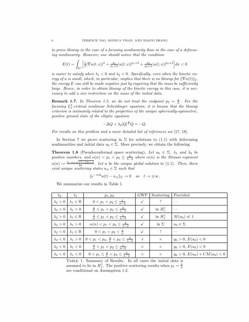
We summarize our results in Table 1.
λ2 λ1 p1, p2 GWP Scattering Provided
λ2 > 0 λ1 ∈ R 0 < p1 < p2 ≤ 4n−2 X ? —
λ2 > 0 λ1 > 0 4n ≤ p1 < p2 ≤ 4
n−2 X in H1x —
λ2 > 0 λ1 ∈ R 4n ≤ p1 < p2 ≤ 4
n−2 X in H1x M(u0) ≪ 1
λ2 > 0 λ1 > 0 α(n) < p1 < p2 ≤ 4n−2 X in Σ u0 ∈ Σ
λ2 < 0 λ1 ∈ R 0 < p1 < p2 < 4n X ? —
λ2 < 0 λ1 > 0 0 < p1 < p2,4n < p2 ≤ 4
n−2 × × y0 > 0, E(u0) < 0
λ2 < 0 λ1 < 0 4n < p1 < p2 ≤ 4
n−2 × × y0 > 0, E(u0) < 0
λ2 < 0 λ1 < 0 0 < p1 ≤ 4n < p2 ≤ 4
n−2 × × y0 > 0, E(u0) + CM(u0) < 0
Table 1. Summary of Results. In all cases the initial data isassumed to lie in H1
x. The positive scattering results when p1 = 4n
are conditional on Assumption 1.2.
NLS WITH COMBINED POWER-TYPE NONLINEARITIES 7
2. Preliminaries
We will often use the notation X . Y whenever there exists some constant Cso that X ≤ CY ; as before, C can depend on n, p1, p2, λ1, λ2. Similarly, we willuse X ∼ Y if X . Y . X . We use X ≪ Y if X ≤ cY for some small constant c.The derivative operator ∇ refers to the space variable only. We will occasionallyuse subscripts to denote spatial derivatives and will use the summation conventionover repeated indices.
We use Lrx(R
n) to denote the Banach space of functions f : Rn → C whose norm
‖f‖r :=(∫
Rn
|f(x)|rdx) 1
r
is finite, with the usual modifications when r = ∞, and identifying functions whichagree almost everywhere. For any non-negative integer k, we denote by W k,r(Rn)the Sobolev space defined as the closure of test functions in the norm
‖f‖Wk,r(Rn) :=∑
|α|≤k
∥∥∥ ∂α
∂xαf∥∥∥r.
We use LqtL
rx to denote the spacetime norm
‖u‖LqtL
rx(R×Rn) :=
(∫
R
(∫
Rn
|u(t, x)|rdx)q/r
dt)1/q
,
with the usual modifications when q or r is infinity, or when the domain R × Rn
is replaced by some smaller spacetime region. When q = r we abbreviate LqtL
rx by
Lqt,x.We define the Fourier transform on Rn to be
f(ξ) :=
∫
Rn
e−2πix·ξf(x)dx.
We will make use of the fractional differentiation operators |∇|s defined by
|∇|sf(ξ) := |ξ|sf(ξ).
These define the homogeneous Sobolev norms
‖f‖Hsx:= ‖|∇|sf‖L2
x.
Let eit∆ be the free Schrodinger propagator. In physical space this is given bythe formula
eit∆f(x) =1
(4πit)n/2
∫
Rn
ei|x−y|2/4tf(y)dy
for t 6= 0 (using a suitable branch cut to define (4πit)n/2), while in frequency spaceone can write this as
(2.1) eit∆f(ξ) = e−4π2it|ξ|2 f(ξ).
In particular, the propagator obeys the dispersive inequality
(2.2) ‖eit∆f‖L∞x
. |t|−n2 ‖f‖L1
x
for all times t 6= 0.We also recall Duhamel’s formula
u(t) = ei(t−t0)∆u(t0)− i
∫ t
t0
ei(t−s)∆(iut +∆u)(s)ds.(2.3)
8 TERENCE TAO, MONICA VISAN, AND XIAOYI ZHANG
We say that a pair of exponents (q, r) is Schrodinger-admissible if 2q +
nr = n
2 and
2 ≤ q, r ≤ ∞. If I × Rn is a spacetime slab, we define the S0(I × Rn) Strichartznorm by
(2.4) ‖u‖S0(I×Rn) := sup ‖u‖LqtL
rx(I×Rn)
where the sup is taken over all admissible pairs (q, r). We define the S1(I × Rn)Strichartz norm to be
‖u‖S1(I×Rn) := ‖∇u‖S0(I×Rn).
We also use N0(I × Rn) to denote the dual space of S0(I × Rn) and
N1(I × Rn) := u; ∇u ∈ N0(I × R
n).
By definition and Sobolev embedding, we obtain
Lemma 2.1. For any S1 function u on I × Rn, we have
‖∇u‖L∞t L2
x+ ‖∇u‖
L
2(n+2)n−2
t L
2n(n+2)
n2+4x
+ ‖∇u‖L
2(n+2)n
t,x
+ ‖∇u‖L2
tL2n
n−2x
+ ‖u‖L∞
t L2n
n−2x
+ ‖u‖L
2(n+2)n−2
t,x
+ ‖u‖L
2(n+2)n
t L
2n(n+2)
n2−2n−4x
. ‖u‖S1
where all spacetime norms are on I × Rn.
Let us also record the following standard Strichartz estimates that we will invokethroughout the paper (for a proof see [14]):
Lemma 2.2. Let I be a compact time interval, k = 0, 1, and let u : I × Rn → C
be an Sk solution to the forced Schrodinger equation
iut +∆u = F
for a function F . Then we have
(2.5) ‖u‖Sk(I×Rn) . ‖u(t0)‖Hk(Rn) + ‖F‖Nk(I×Rn),
for any time t0 ∈ I.
We will also need some Littlewood-Paley theory. Specifically, let ϕ(ξ) be asmooth bump supported in the ball |ξ| ≤ 2 and equalling one on the ball |ξ| ≤ 1.For each dyadic number N ∈ 2Z we define the Littlewood-Paley operators
P≤Nf(ξ) := ϕ(ξ/N)f(ξ),
P>Nf(ξ) := [1− ϕ(ξ/N)]f (ξ),
PNf(ξ) := [ϕ(ξ/N)− ϕ(2ξ/N)]f(ξ).
Similarly we can define P<N , P≥N , and PM<·≤N := P≤N −P≤M , whenever M andN are dyadic numbers. We will frequently write f≤N for P≤Nf and similarly forthe other operators. We recall some standard Bernstein type inequalities:
NLS WITH COMBINED POWER-TYPE NONLINEARITIES 9
Lemma 2.3. For any 1 ≤ p ≤ q ≤ ∞ and s > 0, we have
‖P≥Nf‖Lpx. N−s‖|∇|sP≥Nf‖Lp
x
‖|∇|sP≤Nf‖Lpx. Ns‖P≤Nf‖Lp
x
‖|∇|±sPNf‖Lpx∼ N±s‖PNf‖Lp
x
‖P≤Nf‖Lqx. N
np−n
q ‖P≤Nf‖Lpx
‖PNf‖Lqx. N
np−n
q ‖PNf‖Lpx.
For our analysis and the sake of the exposition, it is convenient to introduce anumber of function spaces. We will need the following Strichartz spaces defined ona slab I × Rn as the closure of the test functions under the appropriate norms:
‖u‖V (I) := ‖u‖L
2(n+2)n
t,x (I×Rn)
‖u‖W (I) := ‖u‖L
2(n+2)n−2
t,x (I×Rn)
‖u‖Z(I) := ‖u‖Ln+1
t L
2(n+1)n−1
x (I×Rn)
.
Definition 2.4. Let I × Rn be an arbitrary spacetime slab. For 0 < p1 < p2 < 4n−2 ,
we define the space
X0(I) := ∩i=1,2Lγi
t Lρix (I × R
n),
and
X1(I) := u; ∇u ∈ X0(I), X1(I) := X0(I) ∩ X1(I),
where γi := 4(pi+2)pi(n−2) , ρi := n(pi+2)
n+pi. It is not hard to check that (γi, ρi) is a
Schrodinger admissible pair and thus S0 ⊂ X0.In the case 0 < p1 < p2 = 4
n−2 , we define the spaces
X0(I) := Lγ1
t Lρ1x (I × R
n) ∩ L2(n+2)n−2
t L2n(n+2)
n2+4x (I × R
n) ∩ V (I)
and
X1(I) := u; ∇u ∈ X0(I), X1(I) := X0(I) ∩ X1(I).
Define ρ∗i := n(pi+2)n−2 and let γ′
i, ρ′i be the dual the exponents of γi, respectively
ρi introduced in Definition 2.4. It is easy to verify that the following identities hold:
1
γ′i
= 1−pi(n− 2)
4+
pi + 1
γ(2.6)
1
ρ′i=
1
ρi+
p
ρ∗i(2.7)
1
ρ∗i=
1
ρi−
1
n.(2.8)
Using (2.6) through (2.8) as well as Holder and Sobolev embedding, we derivethe first estimates for our nonlinearity.
Lemma 2.5. Let I be a compact time interval, 0 < p1 < p2 ≤ 4n−2 , λ1 and λ2 be
nonzero real numbers, and k = 0, 1. Then,∥∥λ1|u|
p1u+ λ2|u|p2u
∥∥Nk(I×Rn)
.∑
i=1,2
|I|1−pi(n−2)
4 ‖u‖pi
X1(I)‖u‖Xk(I)
10 TERENCE TAO, MONICA VISAN, AND XIAOYI ZHANG
and∥∥(λ1|u|
p1u+ λ2|u|p2u
)−(λ1|v|
p1v + λ2|v|p2v
)∥∥N0(I×Rn)
.∑
i=1,2
|I|1−pi(n−2)
4
(‖u‖pi
X1(I)+ ‖v‖pi
X1(I)
)‖u− v‖X0(I).
When the length of the time interval I is infinite, the estimates in Lemma 2.5are useless. In this case we will use instead the following
Lemma 2.6. Let I × Rn be an arbitrary spacetime slab, 4n ≤ p ≤ 4
n−2 , and k = 0, 1.Then
(2.9) ‖|u|pu‖Nk(I×Rn) . ‖u‖2−p(n−2)
2
V (I) ‖u‖np2 −2
W (I) ‖|∇|ku‖V (I).
Proof. By the boundedness of the Riesz potentials on any Lpx, 1 < p < ∞, Holder,
and interpolation, we estimate
‖|u|pu‖Nk(I×Rn) .∥∥|∇|k(|u|pu)
∥∥L
2(n+2)n+4
t,x (I×Rn)
. ‖|u|p‖L
n+22
t,x (I×Rn)‖|∇|ku‖
L2(n+2)
nt,x (I×Rn)
. ‖u‖p
L(n+2)p
2t,x (I×Rn)
‖|∇|ku‖L
2(n+2)n
t,x (I×Rn)
. ‖u‖2−p(n−2)
2
L2(n+2)
nt,x (I×Rn)
‖u‖np2 −2
L
2(n+2)n−2
t,x (I×Rn)
‖|∇|ku‖L
2(n+2)n
t,x (I×Rn),
which proves (2.9).
When deriving global spacetime bounds that imply scattering, we would liketo involve the Z-norm which corresponds to the control given by the a priori in-teraction Morawetz estimate. For k = 0, 1 and 4
n < p < 4n−2 , applying Holder’s
inequality we estimate∥∥|∇|k(|u|pu)
∥∥L2
tL2n
n+2x (I×Rn)
. ‖|∇|ku‖L2
tL2n
n−2x (I×Rn)
‖u‖pL∞
t Lnp2
x (I×Rn)
. ‖|∇|ku‖L2
tL2n
n−2x (I×Rn)
‖u‖2−p(n−2)
2
L∞t L2
x(I×Rn)‖u‖np−4
2
L∞t L
2nn−2x (I×Rn)
.
In order to use the a priori Ln+1t L
2(n+1)n−1
x control (given to us by the interactionMorawetz estimate in the case when both nonlinearities are defocusing), we would
like to replace the L∞t L
np2x -norm by a norm which belongs to the open triangle deter-
mined by the mass (L∞t L2
x), the potential energy (L∞t L
2nn−2x ), and the Ln+1
t L
2(n+1)n−1
x -
norm. This can be achieved by increasing the time exponent in the L2tW
k, 2nn−2
x -normby a tiny amount, while maintaining the scaling (by which we mean replacing thepair (2, 2n
n−2 ) by another Schrodinger-admissible pair). We obtain the following
NLS WITH COMBINED POWER-TYPE NONLINEARITIES 11
Lemma 2.7. Let k = 0, 1 and 4n < p < 4
n−2 . Then, there exists θ > 0 large enoughsuch that on every slab I × Rn we have
∥∥|∇|k(|u|pu)∥∥L2
tL2n
n+2x
. ‖|∇|ku‖L
2+1θ
t L
2n(2θ+1)n(2θ+1)−4θx
‖u‖n+1
2(2θ+1)
Ln+1t L
2(n+1)n−1
x
‖u‖α(θ)L∞
t L2x‖u‖
β(θ)
L∞t L
2nn−2x
. ‖u‖Sk(I×Rn)‖u‖n+1
2(2θ+1)
Z(I) ‖u‖α(θ)L∞
t L2x‖u‖
β(θ)
L∞t L
2nn−2x
,(2.10)
where
α(θ) := p(1− n
2
)+ 8θ+1
2(2θ+1) and β(θ) := n2
(p− n+8θ+2
n(2θ+1)
).
Proof. First note that the pair (2 + 1θ ,
2n(2θ+1)n(2θ+1)−4θ ) is Schrodinger-admissible.
Once α(θ) and β(θ) are positive, (2.10) is a direct consequence of Holder’s in-equality, as the reader can easily check. It is not hard to see that θ 7→ α(θ) andθ 7→ β(θ) are increasing functions and moreover,
α(θ) → p(1− n2 ) + 2 and β(θ) → n
2 (p−4n ) as θ → ∞.
As 4n < p < 4
n−2 , the two limits are positive. Thus, for θ sufficiently large we obtain
α(θ) > 0 and β(θ) > 0.
This concludes the proof of the lemma.
When p = 4n−2 , we can still control the N0-norm of |u|pu in terms of the Z-norm.
The idea is simple: Note that by Holder, we have
‖|u|4
n−2u‖N0(I×Rn) . ‖|u|4
n−2u‖L2
tL2n
n+2x (I×Rn)
. ‖u‖L2
tL2n
n−2x (I×Rn)
‖u‖4
n−2
L∞t L
2nn−2x (I×Rn)
.(2.11)
In order to get a small fractional power of ‖u‖Z(I) on the right-hand side of (2.11),we need to perturb the above estimate a little bit. More precisely, we will replace
the norm L2tL
2nn−2x by L2+ε
t L2n
n−2−εx for a small constant ε > 0. The latter norm inter-
polates between the S0-norm L2+εt L
2n(2+ε)n(2+ε)−4x and the S1-norm L2+ε
t L2n(2+ε)
n(2+ε)−2(4+ε)x ,
provided ε is sufficiently small. Thus,
‖u‖L2+ε
t L2n
n−2−εx (I×Rn)
. ‖u‖S1(I×Rn),(2.12)
provided ε is chosen sufficiently small. Keeping the L2tL
2nn+2x -norm on the left-hand
side of (2.11), this change forces us to replace the norm L∞t L
2nn−2x (which appears on
the right-hand side of (2.11)) with a norm which lies in the open triangle determined
by the potential energy (L∞t L
2nn−2x ), the mass (L∞
t L2x), and the Z-norm. Therefore,
we have the following
Lemma 2.8. Let I × Rn be a spacetime slab. Then, there exists a small constant0 < θ < 1 such that
‖|u|4
n−2u‖N0(I×Rn) . ‖u‖θZ(I)‖u‖n+2n−2−θ
S1(I×Rn).(2.13)
12 TERENCE TAO, MONICA VISAN, AND XIAOYI ZHANG
Proof. We will in fact prove the following estimate
‖|u|4
n−2u‖L2
tL2n
n+2x
. ‖u‖L2+ε
t L2n
n−2−εx
‖u‖(n+1)ε2(2+ε)
Z(I) ‖u‖a(ε)L∞
t L2x‖u‖
b(ε)
L∞t L
2nn−2x
,(2.14)
which holds for ε > 0 sufficiently small. Here, all spacetime norms are on the slabI × Rn and
a(ε) :=(1 + ε)ε
2(2 + ε)and b(ε) :=
4
n− 2−
(n+ 2 + ε)ε
2(2 + ε).
In order to prove (2.14), we just need to check that for ε > 0 sufficiently small,a(ε) and b(ε) are positive, since then the estimate is a simple consequence of Holder’sinequality.
It is easy to see that as functions of ε, a is increasing and a(0) = 0, while b isdecreasing and b(0) = 4
n−2 . Thus, taking ε > 0 sufficiently small, we have a(ε) > 0
and b(ε) > 0, which yields (2.14) for the reasons discussed above.
Taking θ := (n+1)ε2(2+ε) and using (2.12), we obtain (2.13).
Remark 2.9. An easy consequence of (2.14) are estimates for nonlinearities of
the form |u|4
n−2 v. More precisely, on every spacetime slab I × Rn we have
‖|u|4
n−2 v‖N0(I×Rn) . ‖u‖θZ(I)‖u‖4
n−2−θ
S1(I×Rn)‖v‖S1(I×Rn)
and
‖|u|4
n−2 v‖N0(I×Rn) . ‖v‖θZ(I)‖u‖4
n−2
S1(I×Rn)‖v‖1−θS1(I×Rn).
3. Local theory
In this section we present the local theory for the initial value problem (1.1). Westart by recording the local well-posedness statements. As the material is classical,we prefer to omit the proofs and instead send the reader to the detailed expositionsin [4, 5, 12, 13].
Proposition 3.1 (Local well-posedness for (1.1) with H1x-subcritical nonlineari-
ties).Let u0 ∈ H1
x, λ1 and λ2 be nonzero real constants, and 0 < p1 < p2 < 4n−2 . Then,
there exists T = T (‖u0‖H1x) such that (1.1) with the parameters given above admits
a unique strong H1x-solution u on [−T, T ]. Let (−Tmin, Tmax) be the maximal time
interval on which the solution u is well-defined. Then, u ∈ S1(I × Rn) for everycompact time interval I ⊂ (−Tmin, Tmax) and the following properties hold:• If Tmax < ∞, then
limt→Tmax
‖u(t)‖H1x= ∞;
similarly, if Tmin < ∞, then
limt→−Tmin
‖u(t)‖H1x= ∞.
• The solution u depends continuously on the initial data u0 in the following sense:
There exists T = T (‖u0‖H1x) such that if u
(m)0 → u0 in H1
x and if u(m) is the solution
to (1.1) with initial data u(m)0 , then u(m) is defined on [−T, T ] for m sufficiently
large and u(m) → u in S1([−T, T ]× Rn).
NLS WITH COMBINED POWER-TYPE NONLINEARITIES 13
Proposition 3.2 (Local well-posedness for (1.1) with a H1x-critical nonlinearity).
Let u0 ∈ H1x, λ1 and λ2 be nonzero real constants, and 0 < p1 < p2 = 4
n−2 . Then,
for every T > 0, there exists η = η(T ) such that if
‖eit∆u0‖X1([−T,T ]) ≤ η,
then (1.1) with the parameters given above admits a unique strong H1x-solution
u defined on [−T, T ]. Let (−Tmin, Tmax) be the maximal time interval on whichu is well-defined. Then, u ∈ S1(I × Rn) for every compact time interval I ⊂(−Tmin, Tmax) and the following properties hold:• If Tmax < ∞, then
either limt→Tmax
‖u(t)‖H1x= ∞ or ‖u‖S1((0,Tmax)×Rn) = ∞.
Similarly, if Tmin < ∞, then
either limt→−Tmin
‖u(t)‖H1x= ∞ or ‖u‖S1((−Tmin,0)×Rn) = ∞.
• The solution u depends continuously on the initial data u0 in the following sense:The functions Tmin and Tmax are lower semicontinuous from H1
x to (0,∞]. More-
over, if u(m)0 → u0 in H1
x and if u(m) is the maximal solution to (1.1) with initial
data u(m)0 , then u(m) → u in Lq
tH1x([−S, T ]×Rn) for every q < ∞ and every interval
[−S, T ] ⊂ (−Tmin, Tmax).
We record also the following companion to Proposition 3.2.
Lemma 3.3 (Blowup criterion). Let u0 ∈ H1x and let u be the unique strong H1
x-solution to (1.1) with p2 = 4
n−2 on the slab [0, T0]× Rn such that
‖u‖X1([0,T0])< ∞.
Then, there exists δ = δ(u0) > 0 such that the solution u extends to a strongH1
x-solution on the slab [0, T0 + δ]× Rn.
The proof is standard (see, for example, [5]). In the contrapositive, this lemmaasserts that if a solution cannot be continued strongly beyond a time T0, then theX1-norm (and all other S1-norms) must blow up at that time.
Next, we will establish a stability result for the L2x-critical NLS, by which we
mean the following property: Given an approximate solutionivt +∆v = |v|
4n v + e
v(0, x) = v0(x) ∈ L2(Rn)
to (1.7), with e small in a suitable space and v0 − v0 small in L2x, there exists a
genuine solution v to (1.7) which stays very close to v in L2x-critical norms.
Lemma 3.4 (Short-time perturbations). Let I be a compact interval and let v bean approximate solution to (1.7) in the sense that
(i∂t +∆)v = |v|4n v + e,
for some function e. Assume that
‖v‖L∞t L2
x(I×Rn) ≤ M(3.1)
14 TERENCE TAO, MONICA VISAN, AND XIAOYI ZHANG
for some positive constant M . Let t0 ∈ I and let v(t0) close to v(t0) in the sensethat
‖v(t0)− v(t0)‖L2x≤ M ′(3.2)
for some M ′ > 0. Assume also the smallness conditions
‖v‖V (I) ≤ ε0(3.3)∥∥ei(t−t0)∆
(v(t0)− v(t0)
)∥∥V (I)
≤ ε(3.4)
‖e‖N0(I×Rn) ≤ ε,(3.5)
for some 0 < ε ≤ ε0 where ε0 = ε0(M,M ′) > 0 is a small constant. Then, thereexists a solution v to (1.7) on I × Rn with initial data v(t0) at time t = t0 satisfying
‖v − v‖V (I) . ε(3.6)
‖v − v‖S0(I×Rn) . M ′(3.7)
‖v‖S0(I×Rn) . M +M ′(3.8)
‖(i∂t +∆)(v − v) + e‖N0(I×Rn) . ε.(3.9)
Remark 3.5. Note that by Strichartz,∥∥ei(t−t0)∆
(v(t0)− v(t0)
)∥∥V (I)
. ‖v(t0)− v(t0)‖L2x,
so the hypothesis (3.4) is redundant if M ′ = O(ε).
Proof. By time symmetry, we may assume t0 = inf I. Let z := v − v. Then zsatisfies the following initial value problem
izt +∆z = |v + z|
4n (v + z)− |v|
4n v − e
z(t0) = v(t0)− v(t0).
For t ∈ I define
S(t) := ‖(i∂t +∆)z + e‖N0([t0,t]×Rn).
By (3.3), we have
S(t) . ‖(i∂t +∆)z + e‖L
2(n+2)n+4
t,x ([t0,t]×Rn)
. ‖z‖1+ 4
n
V ([t0,t])+ ‖z‖V ([t0,t])‖v‖
4n
V ([t0,t])
. ‖z‖1+ 4
n
V ([t0,t])+ ε
4n
0 ‖z‖V ([t0,t]).(3.10)
On the other hand, by Strichartz, (3.4), and (3.5), we get
‖z‖V ([t0,t]) . ‖ei(t−t0)∆z(t0)‖V ([t0,t]) + S(t) + ‖e‖N0([t0,t]×Rn)
. S(t) + ε.(3.11)
Combining (3.10) and (3.11), we obtain
S(t) . (S(t) + ε)1+4n + ε
4n
0 (S(t) + ε) + ε.
A standard continuity argument then shows that if ε0 = ε0(M,M ′) is taken suffi-ciently small, then
S(t) ≤ ε for any t ∈ I,
NLS WITH COMBINED POWER-TYPE NONLINEARITIES 15
which implies (3.9). Using (3.9) and (3.11), one easily derives (3.6). Moreover, byStrichartz, (3.2), (3.5), and (3.9),
‖z‖S0(I×Rn) . ‖z(t0)‖L2x+ ‖(i∂t +∆)z + e‖N0(I×Rn) + ‖e‖N0([t0,t]×Rn)
. M ′ + ε,
which establishes (3.7).To prove (3.8), we use Strichartz, (3.1), (3.2), (3.3), (3.5), and (3.9):
‖v‖S0(I×Rn) . ‖v(t0)‖L2x+ ‖(i∂t +∆)v‖N0(I×Rn)
. ‖v(t0)‖L2x+ ‖v(t0)− v(t0)‖L2
x+ ‖(i∂t +∆)(v − v) + e‖N0(I×Rn)
+ ‖(i∂t +∆)v‖N0(I×Rn) + ‖e‖N0(I×Rn)
. M +M ′ + ε+ ‖(i∂t +∆)v‖L
2(n+2)n+4
t,x (I×Rn)
. M +M ′ + ‖v‖1+ 4
n
V (I)
. M +M ′ + ε1+ 4
n
0
. M +M ′.
Building upon the previous lemma, we have the following
Lemma 3.6 (L2x-critical stability result). Let I be a compact interval and let v be
an approximate solution to (1.7) in the sense that
(i∂t +∆)v = |v|4n v + e,
for some function e. Assume that
‖v‖L∞t L2
x(I×Rn) ≤ M(3.12)
‖v‖V (I) ≤ L(3.13)
for some positive constants M and L. Let t0 ∈ I and let v(t0) close to v(t0) in thesense that
‖v(t0)− v(t0)‖L2x≤ M ′(3.14)
for some M ′ > 0. Moreover, assume the smallness conditions∥∥ei(t−t0)∆
(v(t0)− v(t0)
)∥∥V (I)
≤ ε(3.15)
‖e‖N0(I×Rn) ≤ ε,(3.16)
for some 0 < ε ≤ ε1 where ε1 = ε1(M,M ′, L) > 0 is a small constant. Then, thereexists a solution v to (1.7) on I × Rn with initial data v(t0) at time t = t0 satisfying
‖v − v‖V (I) ≤ εC(M,M ′, L)(3.17)
‖v − v‖S0(I×Rn) ≤ C(M,M ′, L)M ′(3.18)
‖v‖S0(I×Rn) ≤ C(M,M ′, L).(3.19)
Remark 3.7. By Strichartz, the hypothesis (3.15) is redundant if M ′ = O(ε);see Remark 3.5. Assumption 1.2 is not explicitly used in the proof of this lemma,although in practice one needs an assumption like this if one wishes to obtain thehypothesis (3.13).
16 TERENCE TAO, MONICA VISAN, AND XIAOYI ZHANG
Proof. Subdivide I into N ∼ (1 + Lε0)
2(n+2)n subintervals Ij = [tj , tj+1] such that
‖v‖V (Ij) ∼ ε0,
where ε0 = ε0(M, 2M ′) is as in Lemma 3.4. We need to replace M ′ by 2M ′ as themass of the difference v − v might grow slightly in time.
Choosing ε1 sufficiently small depending on N , M , and M ′, we can applyLemma 3.4 to obtain for each j and all 0 < ε < ε1
‖v − v‖V (Ij) . C(j)ε
‖v − v‖S0(Ij×Rn) . C(j)M ′
‖v‖S0(Ij×Rn) . C(j)(M +M ′)
‖(i∂t +∆)(v − v) + e‖N0(Ij×Rn) . C(j)ε,
provided we can prove that (3.14) and (3.15) hold with t0 replaced by tj . In orderto verify this, we use an inductive argument. By Strichartz, (3.14), (3.16), and theinductive hypothesis,
‖v(tj)− v(tj)‖L2x. ‖v(t0)− v(t0)‖L2
x+ ‖(i∂t +∆)(v − v) + e‖N0([t0,tj]×Rn)
+ ‖e‖N0([t0,tj]×Rn)
. M ′ +j∑
k=0
C(k)ε+ ε.
Similarly, by Strichartz, (3.15), (3.16), and the inductive hypothesis,∥∥ei(t−tj)∆
(v(tj)− v(tj)
)∥∥V (I)
.∥∥ei(t−t0)∆
(v(t0)− v(t0)
)∥∥V (I)
+‖e‖N0([t0,tj]×Rn)
+ ‖(i∂t +∆)(v − v) + e‖N0([t0,tj]×Rn)
. ε+
j∑
k=0
C(k)ε.
Here, C(k) depends on k, M , M ′, and ε0. Choosing ε1 sufficiently small dependingon N , M , and M ′, we can continue the inductive argument.
The corresponding stability result for the H1x-critical NLS in dimensions 3 ≤
n ≤ 6 is derived by similar techniques as the ones presented above. However, thehigher dimensional case, n > 6, is more delicate as derivatives of the nonlinearity aremerely Holder continuous of order 4
n−2 rather than Lipschitz. A stability theory for
the H1x-critical NLS in higher dimensions was established by the first two authors,
[27]. They made use of exotic Strichartz estimates and fractional chain rule typeestimates in order to avoid taking a full derivative, but still remain energy-criticalwith respect to the scaling3. We record their result below.
Lemma 3.8 (H1x-critical stability result). Let I be a compact time interval and let
w be an approximate solution to (1.5) on I × Rn in the sense that
(i∂t +∆)w = |w|4
n−2 w + e
3A very similar technique was employed by K. Nakanishi, [22], for the energy-critical non-linearKlein-Gordon equation in high dimensions.
NLS WITH COMBINED POWER-TYPE NONLINEARITIES 17
for some function e. Assume that
‖w‖W (I) ≤ L(3.20)
‖w‖L∞t H1
x(I×Rn) ≤ E0(3.21)
for some constants L,E0 > 0. Let t0 ∈ I and let w(t0) close to w(t0) in the sensethat
‖w(t0)− w(t0)‖H1x≤ E′(3.22)
for some E′ > 0. Assume also the smallness conditions(∑
N
‖PN∇ei(t−t0)∆(w(t0)− w(t0)
)‖2
L
2(n+2)n−2
t L
2n(n+2)
n2+4x (I×Rn)
)1/2
≤ ε(3.23)
‖∇e‖N0(I×Rn) ≤ ε(3.24)
for some 0 < ε ≤ ε2, where ε2 = ε2(E0, E′, L) is a small constant. Then, there
exists a solution w to (1.5) on I × Rn with the specified initial data w(t0) at timet = t0 satisfying
‖∇(w − w)‖L
2(n+2)n−2
t L
2n(n+2)
n2+4x (I×Rn)
≤ C(E0, E′, L)
(ε+ ε
7(n−2)2
)(3.25)
‖w − w‖S1(I×Rn) ≤ C(E0, E′, L)
(E′ + ε+ ε
7(n−2)2
)(3.26)
‖w‖S1(I×Rn) ≤ C(E0, E′, L).(3.27)
Here, C(E0, E′, L) > 0 is a non-decreasing function of E0, E
′, L, and the dimen-sion n.
Remark 3.9. By Strichartz and Plancherel, on the slab I × Rn we have(∑
N
‖PN∇ei(t−t0)∆(w(t0)− w(t0)
)‖2
L
2(n+2)n−2
t L
2n(n+2)
n2+4x (I×Rn)
)1/2
.(∑
N
‖PN∇(w(t0)− w(t0))‖2L∞
t L2x
)1/2
. ‖∇(w(t0)− w(t0))‖L∞
t L2x
. E′,
so the hypothesis (3.23) is redundant if E′ = O(ε).
We end this section with two well-posedness results concerning the L2x-critical
and the H1x-critical nonlinear Schrodinger equations. More precisely, we show that
control of the solution in a specific norm (‖ · ‖V for the L2x-critical NLS and ‖ · ‖W
for the H1x-critical NLS), yields control of the solution in all the S1-norms .
Lemma 3.10. Let k = 0, 1, I be a compact time interval, and let v be the uniquesolution to (1.7) on I × Rn obeying the bound
‖v‖V (I) ≤ L.(3.28)
Then, if t0 ∈ I and v(t0) ∈ Hkx , we have
‖v‖Sk(I×Rn) ≤ C(L)‖v(t0)‖Hkx.(3.29)
18 TERENCE TAO, MONICA VISAN, AND XIAOYI ZHANG
Proof. Subdivide the interval I into N ∼ (1 + Lη )
2(n+2)n subintervals Ij = [tj , tj+1]
such that
‖v‖V (Ij) ≤ η,
where η is a small positive constant to be chosen momentarily. By Strichartz, oneach Ij we obtain
‖v‖Sk(Ij×Rn) . ‖v(tj)‖Hkx+ ‖|∇|k
(|v|
4n v
)‖L
2(n+2)n+4
t,x (Ij×Rn)
. ‖v(tj)‖Hkx+ ‖v‖
4n
V (Ij)‖v‖Sk(Ij×Rn)
. ‖v(tj)‖Hkx+ η
4n ‖v‖Sk(Ij×Rn).
Choosing η sufficiently small, we obtain
‖v‖Sk(Ij×Rn) . ‖v(tj)‖Hkx.
Adding these estimates over all the subintervals Ij , we obtain (3.29).
Lemma 3.11. Let k = 0, 1, I be a compact time interval, and let w be the uniquesolution to (1.5) on I × Rn obeying the bound
‖w‖W (I) ≤ L.(3.30)
Then, if t0 ∈ I and w(t0) ∈ Hkx , we have
‖w‖Sk(I×Rn) ≤ C(L)‖w(t0)‖Hkx.(3.31)
Proof. The proof is similar to that of Lemma 3.10. Subdivide the interval I into
N ∼ (1 + Lη )
2(n+2)n−2 subintervals Ij = [tj , tj+1] such that
‖w‖W (Ij) ≤ η,
where η is a small positive constant to be chosen later. By Strichartz, on each Ijwe obtain
‖w‖Sk(Ij×Rn) . ‖w(tj)‖Hkx+ ‖|∇|k
(|w|
4n−2w
)‖L
2(n+2)n+4
t,x (Ij×Rn)
. ‖w(tj)‖Hkx+ ‖w‖
4n−2
W (Ij)‖w‖Sk(Ij×Rn)
. ‖w(tj)‖Hkx+ η
4n−2 ‖w‖Sk(Ij×Rn).
Choosing η sufficiently small, we obtain
‖w‖Sk(Ij×Rn) . ‖w(tj)‖Hkx.
The conclusion (3.31) follows by adding these estimates over all subintervals Ij .
4. Global well-posedness
Our goal in this section is to prove Theorem 1.1. We shall abbreviate the energyE(u) as E, and the mass M(u) as M .
There are two ingredients to proving the existence of global solutions to (1.1) inthe cases described in Theorem 1.1. One of them is a ‘good’ local well-posednessstatement, by which we mean that the time of existence of an H1
x-solution dependsonly on the H1
x-norm of its initial data. The second ingredient is an a priori bound
on the kinetic energy of the solution, i.e., its H1x-norm. These two ingredients
NLS WITH COMBINED POWER-TYPE NONLINEARITIES 19
together with the conservation of mass are sufficient to yield the existence of globalsolutions via the standard iterative argument.
Before we continue with our proof, we should make a few remarks:The existence of global L2
x-solutions for (1.1) when both nonlinearities are L2x-
subcritical, i.e., 0 < p1 < p2 < 4n , follows from the local theory for these equations
and the conservation of mass. Indeed, the time of existence of local solutions to(1.1) in this case depends only on the L2
x-norm of the initial data and global well-posedness in L2
x follows from the conservation of mass via the standard iterativeargument. For details see [12, 13, 5]. However, we are interested in the existenceof global H1
x-solutions so, in order to iterate, we also need to control the incrementof the kinetic energy in time.
Moreover, while in the case when both nonlinearities are energy-subcritical thetime of existence of H1
x-solutions depends on the H1x-norm of the initial data, in the
presence of an energy-critical nonlinearity, i.e., p2 = 4n−2 , the local theory asserts
that the time of existence for H1x-solutions depends instead on the profile of the
initial data. In order to prove a ‘good’ local well-posedness statement in the lattercase, we will treat the energy-subcritical nonlinearity |u|p1u as a perturbation tothe energy-critical NLS, which is globally wellposed (see [6, 23, 30]).
4.1. Kinetic energy control. In this subsection we prove an a priori bound onthe kinetic energy of the solution, which is uniform over the time of existence andwhich depends only on the energy and the mass of the initial data. More precisely,we prove that for all times t for which the solution is defined, we have
‖u(t)‖H1x≤ C(E,M).(4.1)
As the energy
E(u(t)) =
∫
Rn
[12 |∇u(t, x)|2 + λ1
p1+2 |u(t, x)|p1+2 + λ2
p2+2 |u(t, x)|p2+2
]dx
is conserved, we immediately see that when both λ1 and λ2 are positive, we obtain
‖∇u(t)‖22 . E,
uniformly in time.Whenever λ1 < 0 and λ2 > 0, we remark the inequality
−|λ1|
p1 + 2|u(t, x)|p1+2 +
|λ2|
p2 + 2|u(t, x)|p2+2 ≥ −C(λ1, λ2)|u(t, x)|
2,
which immediately yields
‖∇u(t)‖22 . E +M,
uniformly over the time of existence.When both λ1 and λ2 are negative, the hypotheses of Theorem 1.1 also force
0 < p1 < p2 < 4n . By interpolation and Sobolev embedding, for all times t we
obtain
‖u(t)‖pi+2 . ‖u(t)‖1− pin
2(pi+2)
2 ‖u(t)‖npi
2(pi+2)
2nn−2
. M12−
pin
4(pi+2) ‖∇u(t)‖npi
2(pi+2)
2 ,
where i = 1, 2. Thus,
‖u(t)‖pi+2pi+2 . M1− (n−2)pi
4 ‖∇u(t)‖npi2
2 .(4.2)
20 TERENCE TAO, MONICA VISAN, AND XIAOYI ZHANG
Next, we make use of Young’s inequality,
(4.3) ab . εaq + ε−q′
q bq′
,
valid for any a, b, ε > 0, with 1 < q < ∞ and q′ the dual exponent to q. Taking
a = ‖∇u(t)‖npi2
2 , b = 1, and q = 4npi
, we obtain
‖u(t)‖pi+2pi+2 . M1− (n−2)pi
4 ‖∇u(t)‖pin
22
. M1− (n−2)pi4 (ε‖∇u(t)‖22 + ε
− npi4−pin ).
Choosing ε sufficiently small, more precisely ε = c2M(n−2)pi
2 −2 for some positiveconstant c ≪ 1, we get
‖u(t)‖pi+2pi+2 ≤ c‖∇u(t)‖22 + C(M)
Thus, by the conservation of energy,
‖∇u(t)‖2 ≤ C(E,M)
uniformly in t.
4.2. ‘Good’ local well-posedness. In this subsection we prove a ‘good’ local well-posedness statement for (1.1) in the presence of an energy-critical nonlinearity, i.e.,p2 = 4
n−2 . More precisely, we will find T = T (‖u0‖H1x) such that in this case, (1.1)
admits a unique strong solution u ∈ S1([−T, T ]× Rn) and moreover,
‖u‖S1([−T,T ]×Rn) ≤ C(E,M).(4.4)
In the case when both nonlinearities are energy-subcritical, this is a consequenceof Proposition 3.1. The bound (1.6) follows easily from (4.4) by subdividing theinterval I into subintervals of length T , deriving the corresponding S1-bounds oneach of these subintervals, and finally adding these bounds.
To simplify notation we assume without loss of generality that |λ1| = |λ2| =1. Moreover, by the local theory (see Section 2, specifically Proposition 3.2 and
Lemma 3.3) it suffices to prove a priori X1-bounds on u on a time interval whosesize depends only on the H1
x-norm of the initial data. That is, we may assume thatthere exists a strong solution u to (1.1) with p2 = 4
n−2 on the slab [−T, T ] × Rn
and show that u has finite X1-bounds on this slab as long as T = T (‖u0‖H1x) is
sufficiently small.In establishing this local well-posedness result, our approach is entirely pertur-
bative. More precisely, we view the first nonlinearity |u|p1u as a perturbation tothe energy-critical NLS, which is globally wellposed, [6, 23, 30].
Let therefore w be the unique strong global solution to the energy-critical equa-tion (1.5) with initial data w0 = u0 at time t = 0. By the main results in [6, 23, 30],we know that such a w exists and moreover,
‖w‖S1(R×Rn) ≤ C(‖u0‖H1x).(4.5)
Furthermore, by Lemma 3.11, we also have
‖w‖S0(R×Rn) ≤ C(‖u0‖H1x)‖u0‖L2
x≤ C(E,M).
By time reversal symmetry it suffices to solve the problem forward in time. By(4.5), we can subdivide R+ into J = J(E, η) subintervals Ij = [tj , tj+1] such that
‖w‖X1(Ij)∼ η(4.6)
NLS WITH COMBINED POWER-TYPE NONLINEARITIES 21
for some small η to be specified later.We are only interested in those subintervals Ij that have a nonempty intersection
with [0, T ]. We may assume (renumbering, if necessary) that there exists J ′ < Jsuch that for any 0 ≤ j ≤ J ′ − 1, [0, T ] ∩ Ij 6= ∅. Thus, we can write
[0, T ] = ∪J′−1j=0 ([0, T ] ∩ Ij).
The nonlinear evolution w being small on the interval Ij implies that the free
evolution ei(t−tj)∆w(tj) is small on Ij . Indeed, this follows from Strichartz, Sobolevembedding, and (4.6):
‖ei(t−tj)∆w(tj)‖X1(Ij)≤ ‖w‖X1(Ij)
+ ‖∇(|w|4
n−2w)‖L
2(n+2)n+4
t,x (Ij×Rn)
≤ ‖w‖X1(Ij)+ C‖∇w‖
L2(n+2)
nt,x (Ij×Rn)
‖w‖4
n−2
L
2(n+2)n−2
t,x (Ij×Rn)
≤ η + C‖w‖n+2n−2
X1(Ij)
≤ η + Cηn+2n−2 ,
where C is an absolute constant that depends on the Strichartz constant. Thus,taking η sufficiently small, for any 0 ≤ j ≤ J ′ − 1, we obtain
‖ei(t−tj)∆w(tj)‖X1(Ij)≤ 2η.(4.7)
Next, we use (4.6) and (4.7) to derive estimates on u. On the interval I0, recallingthat u(0) = w(0) = u0, we use Lemma 2.5 to estimate
‖u‖X1(I0)≤ ‖eit∆u0‖X1(I0)
+ C|I0|1− p1(n−2)
4 ‖u‖p1+1
X1(I0)+ C‖u‖
n+2n−2
X1(I0)
≤ 2η + CT 1− (n−2)p14 ‖u‖p1+1
X1(I0)+ C‖u‖
n+2n−2
X1(I0).
Assuming η and T are sufficiently small, a standard continuity argument then yields
‖u‖X1(I0)≤ 4η.(4.8)
Thus, (3.20) holds on I := I0 for L := 4Cη. Moreover, in the previous subsection weproved that (3.21) holds with E0 := C(E,M). Also, as (3.22) holds with E′ := 0,we are in the position to apply the stability result Lemma 3.8 provided the error,which in this case is the first nonlinearity, is sufficiently small. As by Holder and(4.8),
‖∇e‖N0(I0×Rn) . T 1− (n−2)p14 ‖u‖p1+1
X1(I0). T 1− (n−2)p1
4 ηp1+1,(4.9)
we see that by choosing T sufficiently small (depending only on the energy and themass of the initial data), we get
‖∇e‖N0(I0×Rn) < ε,
where ε = ε(E,M) is a small constant to be chosen later. Thus, taking ε sufficientlysmall, the hypotheses of Lemma 3.8 are satisfied, which implies that the conclusionholds. In particular,
‖u− w‖S1(I0×Rn) ≤ C(E,M)εc(4.10)
for a small positive constant c that depends only on the dimension n.
22 TERENCE TAO, MONICA VISAN, AND XIAOYI ZHANG
By Strichartz, (4.10) implies
‖u(t1)− w(t1)‖H1x≤ C(E,M)εc,(4.11)
‖ei(t−t1)∆(u(t1)− w(t1))‖X1(I1)≤ C(E,M)εc.(4.12)
Using (4.7), (4.11), (4.12), and Strichartz, we estimate
‖u‖X1(I1)≤ ‖ei(t−t1)∆u(t1)‖X1(I1)
+ C|I1|1− p1(n−2)
4 ‖u‖p1+1
X1(I1)+ C‖u‖
n+2n−2
X1(I1)
≤ ‖ei(t−t1)∆w(t1)‖X1(I1)+ ‖ei(t−t1)∆(u(t1)− w(t1))‖X1(I1)
+ CT 1−p1(n−2)4 ‖u‖p1+1
X1(I1)+ C‖u‖
n+2n−2
X1(I1)
≤ 2η + C(E,M)εc + CT 1− (n−2)p14 ‖u‖p1+1
X1(I1)+ C‖u‖
n+2n−2
X1(I1).
A standard continuity argument then yields
‖u‖X1(I1)≤ 4η,
provided ε is chosen sufficiently small depending on E and M , which amountsto taking T sufficiently small depending on E and M . Thus (4.9) holds with I0replaced by I1 and we are again in the position to apply Lemma 3.8 on I := I1 toobtain
‖u− w‖S1(I1)≤ C(E,M)εc
2
.
By induction, for every 0 ≤ j ≤ J ′ − 1 we obtain
‖u‖X1(Ij)≤ 4η,(4.13)
provided ε (and hence T ) is sufficiently small depending on the energy and themass of the initial data. Adding (4.13) over all 0 ≤ j ≤ J ′ − 1 and recalling thatJ ′ < J = J(E, η), we get
‖u‖X1([0,T ]) . 4J ′η ≤ C(E).(4.14)
Next, we show that (4.14) implies S1-control over the solution u on the slab[0, T ]× Rn. This type of argument will appear repeatedly in Section 5. Howevereach time, the hypotheses will be slightly different; this is why we choose not toencapsulate it into a lemma.
By Strichartz, Lemma 2.5, (4.1), (4.14), and recalling that T = T (E,M), weobtain
‖u‖S1([0,T ]×Rn) . ‖u0‖H1x+ T 1−p1(n−2)
4 ‖u‖1+p1
X1([0,T ])+ ‖u‖
n+2n−2
X1([0,T ])
≤ C(E,M).(4.15)
Similarly,
‖u‖S0([0,T ]×Rn) . ‖u0‖L2x+ T 1−p1(n−2)
4 ‖u‖p1
X1([0,T ])‖u‖X0([0,T ])
+ ‖u‖4
n−2
X1([0,T ])‖u‖X0([0,T ])
. M12 + C(E,M)‖u‖p1
X1([0,T ])‖u‖S0([0,T ]×Rn)(4.16)
+ ‖u‖4
n−2
X1([0,T ])‖u‖S0([0,T ]×Rn).
NLS WITH COMBINED POWER-TYPE NONLINEARITIES 23
Subdividing [0, T ] into N = N(E,M, δ) subintervals Jk such that
‖u‖X1(Jk)∼ δ
for some small constant δ > 0, the computations that lead to (4.16) now yield
‖u‖S0(Jk×Rn) . M12 + C(E,M)δp1‖u‖S0(Jk×Rn) + δ
4n−2 ‖u‖S0(Jk×Rn).
Choosing δ sufficiently small depending on E and M , we obtain
‖u‖S0(Jk×Rn) ≤ C(E,M)
on every subinterval Jk. Adding these bounds over all subintervals Jk, we get
‖u‖S0([0,T ]×Rn) ≤ C(E,M).(4.17)
Collecting (4.15) and (4.17), we obtain
‖u‖S1([0,T ]) ≤ C(E,M).
This concludes the proof of Theorem 1.1.
5. Scattering results
In this section we prove Theorem 1.3. As before we shall abbreviate the energyE(u) as E, and the mass M(u) as M . The key ingredient is a good spacetimebound; scattering then follows by standard techniques (see subsection 4.8).
In the case when both nonlinearities are defocusing, i.e., λ1, λ2 > 0, an a priorispacetime estimate for the solution is provided by the interaction Morawetz inequal-ity, which we develop in subsection 5.1. In subsections 5.2 through 5.5, we upgradethis bound to a spacetime bound that implies scattering, thus covering Case 1) ofTheorem 1.3. Case 2) is treated in subsections 5.6 and 5.7. In subsection 5.8 weconstruct the scattering states and prove the scattering result.
5.1. The interaction Morawetz inequality. The goal of this subsection is toprove
Proposition 5.1 (Morawetz control). Let I be a compact interval, λ1 and λ2
positive real numbers, and u a solution to (1.1) on the slab I × Rn. Then
‖u‖Ln+1
t L
2(n+1)n−1
x (I×Rn)
. ‖u‖L∞t H1
x(I×Rn).(5.1)
We will derive Proposition 5.1 from the following:
Proposition 5.2 (The interaction Morawetz estimate). Let I be a compact timeinterval and u a solution to (1.1) on the slab I × Rn. Then, we have the followinga priori estimate:
− (n− 1)
∫
I
∫
Rn
∫
Rn
∆(
1|x−y|
)|u(t, y)|2|u(t, x)|2dx dy dt
+∑
i=1,2
2(n− 1)λipipi + 2
∫
I
∫
Rn
∫
Rn
|u(t, y)|2|u(t, x)|pi+2
|x− y|dx dy dt
≤ 4‖u‖4L∞t H1
x(I×Rn).
24 TERENCE TAO, MONICA VISAN, AND XIAOYI ZHANG
Proof. The calculations in this section are difficult to justify without additionalassumptions (particularly, smoothness) of the solution. This obstacle can be dealtwith in the standard manner: mollify the initial data and the nonlinearity to makethe interim calculations valid and observe that the mollifications can be removedat the end using the local well-posedness theory. For clarity, we omit these detailsand keep all computations on a formal level.
We start by recalling the standard Morawetz action centered at a point. Let abe a spatial function and u satisfy
iut +∆u = N(5.2)
on I × Rn. For t ∈ I, we define the Morawetz action centered at zero to be
M0a (t) = 2
∫
Rn
aj(x)Im(u(t, x)uj(t, x))dx.
A computation establishes the following
Lemma 5.3.
∂tM0a =
∫
Rn
(−∆∆a)|u|2 + 4
∫
Rn
ajkRe(ujuk) + 2
∫
Rn
ajN , ujp,
where we define the momentum bracket to be f, gp := Re(f∇g−g∇f) and repeatedindices are implicitly summed.
Note that in the particular case when the nonlinearity is N :=∑
i=1,2 λi|u|piu,
we have N , up = −∑
i=1,2λipi
pi+2∇(|u|pi+2).
Now let a(x) := |x|. For this choice of the function a, one should interpretM0
a as a spatial average of the radial component of the L2x-mass current. Easy
computations show that in dimension n ≥ 3 we have the following identities:
aj(x) =xj
|x|
ajk(x) =δjk|x|
−xjxk
|x|3
∆a(x) =n− 1
|x|
−∆∆a(x) =− (n− 1)∆( 1
|x|
)
and hence
∂tM0a = −(n− 1)
∫
Rn
∆( 1
|x|
)|u(x)|2dx+ 4
∫
Rn
(δjk|x|
−xjxk
|x|3
)Re(ujuk)(x)dx
+ 2
∫
Rn
xj
|x|N , ujp(x)dx
= −(n− 1)
∫
Rn
∆( 1
|x|
)|u(x)|2dx+ 4
∫
Rn
1
|x||∇0u(x)|
2dx
+ 2
∫
Rn
x
|x|N , up(x)dx,
where we use ∇0 to denote the complement of the radial portion of the gradient,that is, ∇0 := ∇− x
|x|(x|x| · ∇).

NLS WITH COMBINED POWER-TYPE NONLINEARITIES 25
We may center the above argument at any other point y ∈ Rn. Choosing a(x) :=|x− y|, we define the Morawetz action centered at y to be
Mya (t) = 2
∫
Rn
x− y
|x− y|Im(u(t, x)∇u(t, x))dx.
The same considerations now yield
∂tMya = −(n− 1)
∫
Rn
∆( 1
|x− y|
)|u(x)|2dx+ 4
∫
Rn
1
|x− y||∇yu(x)|
2dx
+ 2
∫
Rn
x− y
|x− y|N , up(x)dx.
We are now ready to define the interaction Morawetz potential, which is a wayof quantifying how mass is interacting with (moving away from) itself:
M interact(t) :=
∫
Rn
|u(t, y)|2Mya (t)dy
= 2Im
∫
Rn
∫
Rn
|u(t, y)|2x− y
|x− y|∇u(t, x)u(t, x)dx dy.
One obtains immediately the easy estimate
|M interact(t)| ≤ 2‖u(t)‖3L2x‖u(t)‖H1
x.
Calculating the time derivative of the interaction Morawetz potential, we get thefollowing virial-type identity:
∂tMinteract =− (n− 1)
∫
Rn
∫
Rn
∆( 1
|x− y|
)|u(y)|2|u(x)|2dx dy(5.3)
+ 4
∫
Rn
∫
Rn
|u(y)|2|∇yu(x)|2
|x− y|dx dy(5.4)
+ 2
∫
Rn
∫
Rn
|u(y)|2x− y
|x− y|N , up(x)dx dy(5.5)
+ 2
∫
Rn
∂ykIm(uuk)(y)M
ya dy(5.6)
+ 4Im
∫
Rn
∫
Rn
N , um(y)x− y
|x − y|∇u(x)u(x)dx dy,(5.7)
where the mass bracket is defined to be f, gm := Im(f g). Note that for the non-linearity of interest N :=
∑i=1,2 λi|u|piu, we have N , um = 0.
As far as the terms in the above identity are concerned, we will establish
Lemma 5.4. (5.6) ≥ –(5.4).
Thus, integrating with respect to time over a compact interval I, we get
26 TERENCE TAO, MONICA VISAN, AND XIAOYI ZHANG
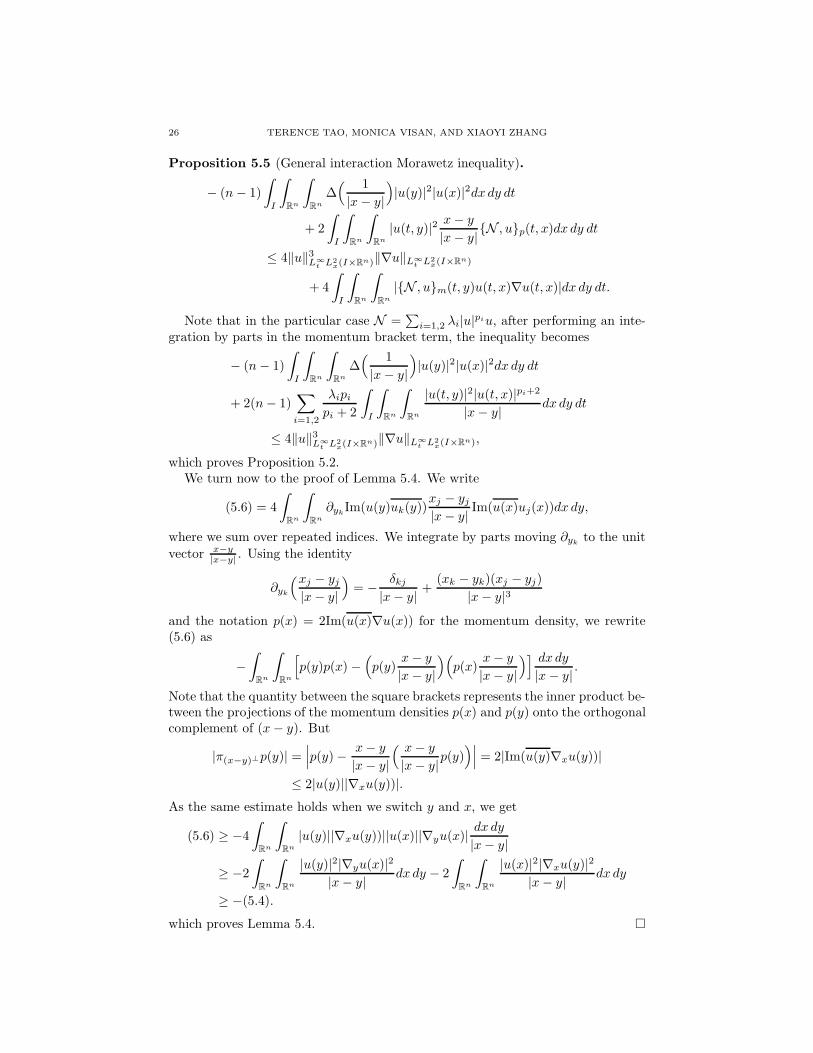
Proposition 5.5 (General interaction Morawetz inequality).
− (n− 1)
∫
I
∫
Rn
∫
Rn
∆( 1
|x− y|
)|u(y)|2|u(x)|2dx dy dt
+ 2
∫
I
∫
Rn
∫
Rn
|u(t, y)|2x− y
|x− y|N , up(t, x)dx dy dt
≤ 4‖u‖3L∞t L2
x(I×Rn)‖∇u‖L∞t L2
x(I×Rn)
+ 4
∫
I
∫
Rn
∫
Rn
|N , um(t, y)u(t, x)∇u(t, x)|dx dy dt.
Note that in the particular case N =∑
i=1,2 λi|u|piu, after performing an inte-
gration by parts in the momentum bracket term, the inequality becomes
− (n− 1)
∫
I
∫
Rn
∫
Rn
∆( 1
|x− y|
)|u(y)|2|u(x)|2dx dy dt
+ 2(n− 1)∑
i=1,2
λipipi + 2
∫
I
∫
Rn
∫
Rn
|u(t, y)|2|u(t, x)|pi+2
|x− y|dx dy dt
≤ 4‖u‖3L∞t L2
x(I×Rn)‖∇u‖L∞t L2
x(I×Rn),
which proves Proposition 5.2.We turn now to the proof of Lemma 5.4. We write
(5.6) = 4
∫
Rn
∫
Rn
∂ykIm(u(y)uk(y))
xj − yj|x− y|
Im(u(x)uj(x))dx dy,
where we sum over repeated indices. We integrate by parts moving ∂ykto the unit
vector x−y|x−y| . Using the identity
∂yk
(xj − yj|x− y|
)= −
δkj|x− y|
+(xk − yk)(xj − yj)
|x− y|3
and the notation p(x) = 2Im(u(x)∇u(x)) for the momentum density, we rewrite(5.6) as
−
∫
Rn
∫
Rn
[p(y)p(x)−
(p(y)
x− y
|x− y|
)(p(x)
x− y
|x− y|
)] dx dy
|x− y|.
Note that the quantity between the square brackets represents the inner product be-tween the projections of the momentum densities p(x) and p(y) onto the orthogonalcomplement of (x− y). But
|π(x−y)⊥p(y)| =∣∣∣p(y)− x− y
|x− y|
( x− y
|x− y|p(y)
)∣∣∣ = 2|Im(u(y)∇xu(y))|
≤ 2|u(y)||∇xu(y))|.
As the same estimate holds when we switch y and x, we get
(5.6) ≥ −4
∫
Rn
∫
Rn
|u(y)||∇xu(y))||u(x)||∇yu(x)|dx dy
|x− y|
≥ −2
∫
Rn
∫
Rn
|u(y)|2|∇yu(x)|2
|x− y|dx dy − 2
∫
Rn
∫
Rn
|u(x)|2|∇xu(y)|2
|x− y|dx dy
≥ −(5.4).
which proves Lemma 5.4.
NLS WITH COMBINED POWER-TYPE NONLINEARITIES 27
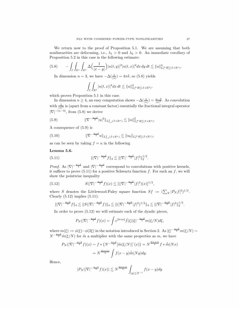
We return now to the proof of Proposition 5.1. We are assuming that bothnonlinearities are defocusing, i.e., λ1 > 0 and λ2 > 0. An immediate corollary ofProposition 5.2 in this case is the following estimate:
−
∫
I
∫
Rn
∫
Rn
∆( 1
|x− y|
)|u(t, y)|2|u(t, x)|2dx dy dt . ‖u‖4L∞
t H1x(I×Rn).(5.8)
In dimension n = 3, we have −∆( 1|x|) = 4πδ, so (5.8) yields
∫
I
∫
R3
|u(t, x)|4dx dt . ‖u‖4L∞t H1
x(I×R3),
which proves Proposition 5.1 in this case.In dimension n ≥ 4, an easy computation shows −∆( 1
|x|) =n−3|x|3 . As convolution
with 1|x|3 is (apart from a constant factor) essentially the fractional integral operator
|∇|−(n−3), from (5.8) we derive
‖∇−n−32 |u|2‖L2
t,x(I×Rn) . ‖u‖2L∞t H1
x(I×Rn).(5.9)
A consequence of (5.9) is
‖∇−n−34 u‖L4
t,x(I×Rn) . ‖u0‖L∞t H1
x(I×Rn),(5.10)
as can be seen by taking f = u in the following
Lemma 5.6.
‖|∇|−n−34 f‖4 . ‖|∇|−
n−32 |f |2‖
1/22 .(5.11)
Proof. As |∇|−n−34 and |∇|−
n−32 correspond to convolutions with positive kernels,
it suffices to prove (5.11) for a positive Schwartz function f . For such an f , we willshow the pointwise inequality
S(|∇|−n−34 f)(x) . [(|∇|−
n−32 |f |2)(x)]1/2,(5.12)
where S denotes the Littlewood-Paley square function Sf := (∑
N |PNf |2)1/2.Clearly (5.12) implies (5.11):
‖|∇|−n−34 f‖4 . ‖S(|∇|−
n−34 f)‖4 . ‖(|∇|−
n−32 |f |2)1/2‖4 . ‖|∇|−
n−32 |f |2‖
1/22 .
In order to prove (5.12) we will estimate each of the dyadic pieces,
PN (|∇|−n−34 f)(x) =
∫e2πixξf(ξ)|ξ|−
n−34 m(ξ/N)dξ,
wherem(ξ) := φ(ξ)−φ(2ξ) in the notation introduced in Section 2. As |ξ|−n−34 m(ξ/N) ∼
N−n−34 m(ξ/N) for m a multiplier with the same properties as m, we have
PN (|∇|−n−34 f)(x) ∼ f ∗
(N−n−3
4 [m(ξ/N)] (x))= N
3(n+1)4 f ∗ ˇm(Nx)
= N3(n+1)
4
∫f(x− y) ˇm(Ny)dy.
Hence,
|PN (|∇|−n−34 f)(x)| . N
3(n+1)4
∫
|y|≤N−1
f(x− y)dy
28 TERENCE TAO, MONICA VISAN, AND XIAOYI ZHANG
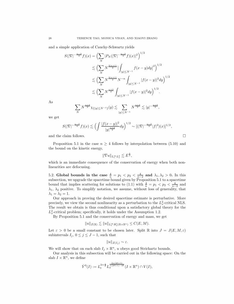
and a simple application of Cauchy-Schwartz yields
S(|∇|−n−34 f)(x) =
(∑
N
|PN (|∇|−n−34 f)(x)|2
)1/2
.(∑
N
N3(n+1)
2
∣∣∫
|y|≤N−1
f(x− y)dy∣∣2)1/2
.(∑
N
N3(n+1)
2 N−n
∫
|y|≤N−1
|f(x− y)|2dy)1/2
.(∑
N
Nn+32
∫
|y|≤N−1
|f(x− y)|2dy)1/2
.
As ∑
N
Nn+32 χ|y|≤N−1(y) .
∑
|y|≤N−1
Nn+32 . |y|−
n+32 ,
we get
S(|∇|−n−34 f)(x) .
(∫ |f(x− y)|2
|y|n+32
dy)1/2
∼ [(|∇|−n−32 |f |2)(x)]1/2,
and the claim follows.
Proposition 5.1 in the case n ≥ 4 follows by interpolation between (5.10) andthe bound on the kinetic energy,
‖∇u‖L∞t L2
x. E
12 ,
which is an immediate consequence of the conservation of energy when both non-linearities are defocusing.
5.2. Global bounds in the case 4n = p1 < p2 < 4
n−2 and λ1, λ2 > 0. In thissubsection, we upgrade the spacetime bound given by Proposition 5.1 to a spacetimebound that implies scattering for solutions to (1.1) with 4
n = p1 < p2 < 4n−2 and
λ1, λ2 positive. To simplify notation, we assume, without loss of generality, thatλ1 = λ2 = 1.
Our approach in proving the desired spacetime estimate is perturbative. Moreprecisely, we view the second nonlinearity as a perturbation to the L2
x-critical NLS.The result we obtain is thus conditional upon a satisfactory global theory for theL2x-critical problem; specifically, it holds under the Assumption 1.2.By Proposition 5.1 and the conservation of energy and mass, we get
‖u‖Z(R) . ‖u‖L∞t H1
x(R×Rn) ≤ C(E,M).
Let ε > 0 be a small constant to be chosen later. Split R into J = J(E,M, ε)subintervals Ij , 0 ≤ j ≤ J − 1, such that
‖u‖Z(Ij) ∼ ε.
We will show that on each slab Ij × Rn, u obeys good Strichartz bounds.Our analysis in this subsection will be carried out in the following space: On the
slab I × Rn, we define
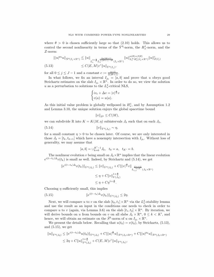
Y 0(I) := L2+ 1
θ
t L2n(2θ+1)
n(2θ+1)−4θx (I × R
n) ∩ V (I),
NLS WITH COMBINED POWER-TYPE NONLINEARITIES 29
where θ > 0 is chosen sufficiently large so that (2.10) holds. This allows us to
control the second nonlinearity in terms of the Y 0-norm, the H1x-norm, and the
Z-norm:
‖|u|p2u‖N0(Ij×Rn) . ‖u‖L
2+1θ
t L
2n(2θ+1)n(2θ+1)−4θx (Ij×Rn)
‖u‖α(θ)+β(θ)L∞
t H1x(Ij×Rn)‖u‖
cZ(Ij)
≤ C(E,M)εc‖u‖Y 0(Ij),(5.13)
for all 0 ≤ j ≤ J − 1 and a constant c := n+12(2θ+1) .
In what follows, we fix an interval Ij0 = [a, b] and prove that u obeys goodStrichartz estimates on the slab Ij0 × Rn. In order to do so, we view the solutionu as a perturbation to solutions to the L2
x-critical NLS,ivt +∆v = |v|
4n v
v(a) = u(a).
As this initial value problem is globally wellposed in H1x, and by Assumption 1.2
and Lemma 3.10, the unique solution enjoys the global spacetime bound
‖v‖S0 ≤ C(M),
we can subdivide R into K = K(M, η) subintervals Jk such that on each Jk,
‖v‖Y 0(Jk)∼ η,(5.14)
for a small constant η > 0 to be chosen later. Of course, we are only interested inthose Jk = [tk, tk+1] which have a nonempty intersection with Ij0 . Without loss ofgenerality, we may assume that
[a, b] = ∪K′−1k=0 Jk, t0 = a, tK′ = b.
The nonlinear evolution v being small on Jk×Rn implies that the linear evolutionei(t−tk)∆v(tk) is small as well. Indeed, by Strichartz and (5.14), we get
‖ei(t−tk)∆v(tk)‖Y 0(Jk)≤ ‖v‖Y 0(Jk)
+ C‖|v|4n v‖
L
2(n+2)n+4
t,x (Jk×Rn)
≤ η + C‖v‖1+ 4
n
V (Jk)
≤ η + Cη1+4n .
Choosing η sufficiently small, this implies
‖ei(t−tk)∆v(tk)‖Y 0(Jk)≤ 2η.(5.15)
Next, we will compare u to v on the slab [t0, t1]×Rn via the L2x-stability lemma
and use the result as an input in the conditions one needs to check in order tocompare u to v (again, via Lemma 3.6) on the slab [t1, t2] × Rn. By iteration, wewill derive bounds on u from bounds on v on all slabs Jk × Rn, 0 ≤ k < K ′, andhence, we will obtain an estimate on the S0-norm of u on Ij0 × Rn.
We present the details below. Recalling that u(t0) = v(t0), by Strichartz, (5.13),and (5.15), we get
‖u‖Y 0(J0)≤ ‖ei(t−t0)∆u(t0)‖Y 0(J0)
+ C‖|u|4nu‖N0(J0×Rn) + C‖|u|p2u‖N0(J0×Rn)
≤ 2η + C‖u‖1+ 4
n
Y 0(J0)+ C(E,M)εc‖u‖Y 0(J0)
,
30 TERENCE TAO, MONICA VISAN, AND XIAOYI ZHANG
which, by a standard continuity argument, yields
‖u‖Y 0(J0)≤ 4η,(5.16)
provided η and ε = ε(E,M) are chosen sufficiently small. Therefore, in order toapply Lemma 3.6, we just need to check that the error term e = |u|p2u is small in
N0(J0 × Rn). As by (5.13),
(5.17) ‖e‖N0(J0×Rn) ≤ C(E,M)εc‖u‖Y 0(J0)≤ C(E,M)ηεc,
choosing ε sufficiently small depending only on E and M , we obtain
‖u− v‖S0(J0×Rn) ≤ εc/2.
By Strichartz, this implies
‖u(t1)− v(t1)‖L2x≤ εc/2,(5.18)
‖ei(t−t1)∆(u(t1)− v(t1))‖Y 0(J1). εc/2.(5.19)
Before turning to the second interval, J1, let us also remark the following S1-control on u on the slab J0 × Rn. Indeed, by Strichartz, (5.13), and (5.16), wehave
‖u‖S1(J0×Rn) . ‖u(a)‖H1x+ ‖u‖
4n
V (J0)‖u‖S1(J0×Rn) + ‖|u|p2u‖N1(J0×Rn)
. C(E) + (4η)4n ‖u‖S1(J0×Rn) + C(E,M)εc‖u‖S1(J0×Rn),
which for η and ε = ε(E,M) sufficiently small yields
‖u‖S1(J0×Rn) ≤ C(E).
Next, we use (5.18) and (5.19) to estimate u on the slab J1×Rn. By Strichartz,(5.13), (5.15), and (5.19), we estimate
‖u‖Y 0(J1)≤ ‖ei(t−t1)∆v(t1)‖Y 0(J1)
+ ‖ei(t−t1)∆(u(t1)− v(t1))‖Y 0(J1)
+ C‖u‖1+ 4
n
Y 0(J1)+ C(E,M)εc‖u‖Y 0(J1)
≤ 2η + εc/2 + C‖u‖1+ 4
n
Y 0(J1)+ C(E,M)εc‖u‖Y 0(J1)
.
A standard continuity argument yields
‖u‖Y 0(J1)≤ 4η,
provided η and ε = ε(E,M) are chosen sufficiently small. This implies that theerror, i.e., |u|p1u, obeys (5.17) with J0 replaced by J1. Choosing ε sufficiently smalldepending on E and M , we can apply Lemma 3.6 to derive
‖u− v‖S0(J1×Rn) ≤ εc/4.
The same arguments as before also yield
‖u‖S1(J1×Rn) ≤ C(E).
By induction, taking ε smaller with each step, for each 0 ≤ k ≤ K ′−1 we obtain
‖u− v‖S0(Jk×Rn) ≤ εc/2k+1
and
‖u‖S1(Jk×Rn) ≤ C(E).
NLS WITH COMBINED POWER-TYPE NONLINEARITIES 31
Adding these estimates over all the intervals Jk which have a nontrivial intersectionwith Ij0 , we obtain
‖u‖S0(Ij0×Rn) . ‖v‖S0(Ij0×Rn) +
K′−1∑
k=0
‖u− v‖S0(Jk×Rn) ≤ C(E,M),
‖u‖S1(Ij0×Rn) .
K′−1∑
k=0
‖u‖S1(Jk×Rn) ≤ C(E,M).
As the interval Ij0 was arbitrarily chosen, we get
‖u‖S0(R×Rn) .
J−1∑
j=0
‖u‖S0(Ij×Rn) . JC(E,M) ≤ C(E,M),
‖u‖S1(R×Rn) .
J−1∑
j=0
‖u‖S1(Ij×Rn) . JC(E,M) ≤ C(E,M),
and hence
‖u‖S1(R×Rn) ≤ C(E,M).
5.3. Ode to Morawetz. In this subsection we upgrade the bound (5.1) to goodStrichartz bounds in the case 4
n < p1 < p2 < 4n−2 and λ1, λ2 positive. For simplicity,
we only derive spacetime bounds for solutions to the initial value problem
(5.20)
iut +∆u = |u|pu
u(0) = u0 ∈ H1x,
with 4n < p < 4
n−2 . Treating the NLS with finitely many such nonlinearitiesintroduces only notational difficulties.
Scattering in H1x for solutions to (5.20) was first proved by J. Ginibre and G.
Velo, [9]. Below, we present a new, simpler proof that relies on the interactionMorawetz estimate.
By Theorem 1.1, the initial value problem (5.20) is globally wellposed. Moreover,by Proposition 5.2 and the conservation of energy (E) and mass (M), the uniqueglobal solution satisfies
‖u‖Ln+1
t L
2(n+1)n−1
x (R×Rn)
. ‖u‖L∞t H1
x(R×Rn) ≤ C(E,M).
Let η > 0 be a small constant to be chosen later and divide R into J = J(E,M, η)subintervals Ij = [tj , tj+1] such that
‖u‖Ln+1
t L2(n+1)n−1
x (Ij×Rn)
∼ η.
Then, on Ij u satisfies the integral equation
u(t) = ei(t−tj)∆u(tj)− i
∫ t
tj
ei(t−s)∆(|u|pu
)(s)ds.
By Strichartz,
‖u‖S1(Ij×Rn) . ‖u(tj)‖H1x+ ‖|u|pu‖
L2tW
1, 2nn+2
x (Ij×Rn),
32 TERENCE TAO, MONICA VISAN, AND XIAOYI ZHANG
which by Lemma 2.7 yields
‖u‖S1(Ij×Rn) . ‖u‖L∞t H1
x(Ij×Rn) + ηn+1
2(2θ+1) ‖u‖α(θ)+β(θ)L∞
t H1x(Ij×Rn)‖u‖S1(Ij×Rn),
provided θ is chosen sufficiently large. From the conservation of energy and mass,and choosing η sufficiently small (depending on E and M), we get
‖u‖S1(Ij×Rn) ≤ C(E,M).
Summing these bounds over all intervals Ij , we obtain
‖u‖S1(R×Rn) . JC(E,M) ≤ C(E,M).
5.4. Global bounds in the case 4n < p1 < p2 = 4
n−2 and λ1, λ2 > 0. In thissubsection we upgrade the spacetime estimate given by the interaction Morawetzinequality, (5.1), to spacetime bounds that imply scattering. The approach is sim-ilar to that used in subsection 5.2; this time, we view the first nonlinearity as aperturbation to the energy-critical NLS. Without loss of generality, we may assumeλ1 = λ2 = 1.
Let ε be a small constant to be chosen later. As by Proposition 5.1 and theconservation of energy and mass,
‖u‖Z(R) = ‖u‖Ln+1
t L
2(n+1)n−1
x (R×Rn)
. ‖u‖L∞t H1
x(R×Rn) ≤ C(E,M),
we can split R into J = J(E,M, ε) intervals Ij , 0 ≤ j ≤ J − 1, such that
‖u‖Z(Ij) ∼ ε.(5.21)
We will show that on each slab Ij × Rn, u obeys good Strichartz bounds.For a spacetime slab I × Rn, we define the spaces
Y 0(I) := L2+ 1
θ
t L2n(2θ+1)
n(2θ+1)−4θx (I × R
n) ∩ L2(n+2)
n
t,x (I × Rn) ∩ L
2(n+2)n−2
t L2n(n+2)
n2+4x (I × R
n),
Y 1(I) := u : ∇u ∈ Y 0(I), and Y 1(I) := Y 0(I) ∩ Y 1(I)
with the usual topology. Here, θ is a sufficiently large constant so that (2.10) holds;that is, on each slab Ij × Rn,
‖∇(|u|p1u
)‖L2
tL2n
n+2x (Ij×Rn)
. ‖∇u‖L
2+1θ
t L
2n(2θ+1)n(2θ+1)−4θx (Ij×Rn)
‖u‖n+1
2(2θ+1)
Z(Ij)‖u‖
α(θ)+β(θ)L∞
t H1x(Ij×Rn)
≤ C(E,M)εn+1
2(2θ+1) ‖u‖Y 1(Ij).(5.22)
Moreover, in this notation we also have (by Sobolev embedding)
‖∇(|u|
4n−2u
)‖L
2(n+2)n+4
t,x (Ij×Rn)
. ‖∇u‖L
2(n+2)n
x,t (Ij×Rn)‖u‖
4n−2
L
2(n+2)n−2
x,t (Ij×Rn)
. ‖u‖n+2n−2
Y 1(Ij),
(5.23)
for each 0 ≤ j ≤ J − 1.Fix Ij0 := [a, b]. On the slab Ij0 × Rn, we treat the first nonlinearity as a
perturbation to the energy-critical NLS
(5.24)
iwt +∆w = |w|
4n−2w
w(a) = u(a).
NLS WITH COMBINED POWER-TYPE NONLINEARITIES 33
By the global well-posedness results in [6, 23, 30], there exists a unique globalsolution w to (5.24) with initial data u(a) at time t = a and moreover,
‖w‖S1(R×Rn) ≤ C(‖u(a)‖H1x) ≤ C(E).(5.25)
By Lemma 3.11, (5.25) implies
‖w‖S0(R×Rn) ≤ C(‖u(a)‖H1x)‖u(a)‖L2
x≤ C(E,M).
Given (5.25), we can split R into K = K(E, η) subintervals Jk = [tk, tk+1] suchthat
‖w‖Y 1(Jk)∼ η,(5.26)
for some small constant η > 0 to be chosen later. Using (5.26) and Strichartz,it is easy to see that the free evolution ei(t−tk)∆w(tk) is small on Jk for every0 ≤ k ≤ K − 1. Indeed,
‖ei(t−tk)∆w(tk)‖Y 1(Jk)≤ ‖w‖Y 1(Jk)
+∥∥∥∫ t
tk
ei(t−s)∆(|w|
4n−2w
)(s)ds
∥∥∥Y 1(Jk)
≤ ‖w‖Y 1(Jk)+ C‖w‖
n+2n−2
Y 1(Jk)
≤ 2η,(5.27)
provided η is chosen sufficiently small.Of course, we are only interested in those Jk that have a nonempty intersection
with Ij0 ; we assume, without loss of generality, that for 0 ≤ k ≤ K ′−1, Jk∩ [a, b] 6=∅, and write
[a, b] = ∪K′−1k=0 Jk = ∪K′−1
k=0 [tk, tk+1], t0 = a, tK′ = b.
We are going to estimate u on each Jk × Rn.First we estimate u on J0×Rn. Noting that w(t0) = w(a) = u(a), by Strichartz,
(5.22), (5.23), (5.26), and (5.27), we get
‖u‖Y 1(J0)≤ ‖ei(t−a)∆u(a)‖Y 1(J0)
+ C(E,M)εn+1
2(2θ+1) ‖u‖Y 1(J0)+ C‖u‖
n+2n−2
Y 1(J0)
≤ 2η + C(E,M)εn+1
2(2θ+1) ‖u‖Y 1(J0)+ C‖u‖
n+2n−2
Y 1(J0).
Choosing η and ε = ε(E,M) sufficiently small, a standard continuity argumentyields
‖u‖Y 1(J0)≤ 4η.
In order to apply Lemma 3.8 on the interval J0, we are left to check that the errorterm e = |u|p1u is small. As by (5.22),
‖∇e‖N0(J0×Rn) ≤ C(E,M)εn+1
2(2θ+1) ‖u‖Y 1(J0)≤ C(E,M)ε
n+12(2θ+1) η,(5.28)
choosing ε sufficiently small (depending only on the energy and the mass), we mayapply Lemma 3.8 to obtain
‖u− w‖S1(J0×Rn) ≤ C(E)εc,
where c = c(n, θ) is a small constant. By the triangle inequality and (5.25), thisimplies
‖u‖S1(J0×Rn) ≤ C(E),
34 TERENCE TAO, MONICA VISAN, AND XIAOYI ZHANG
while by Strichartz, it implies
‖u(t1)− w(t1)‖H1x≤ C(E)εc,
‖ei(t−t1)∆(u(t1)− w(t1))‖Y 1(J1)≤ C(E)εc.(5.29)
Now, we can use these last two estimates to control u on J1. By Strichartz, (5.22),(5.23), (5.27), and (5.29), we get
‖u‖Y 1(J1)≤ ‖ei(t−t1)∆u(t1)‖Y 1(J1)
+ C(E,M)εn+1
2(2θ+1) ‖u‖Y 1(J1)+ C‖u‖
n+2n−2
Y 1(J1)
≤ ‖ei(t−t1)∆w(t1)‖Y 1(J1)+ ‖ei(t−t1)∆(w(t1)− u(t1))‖Y 1(J1)
+ C(E,M)εn+1
2(2θ+1) ‖u‖Y 1(J1)+ C‖u‖
n+2n−2
Y 1(J1)
≤ 2η + C(E)εc + C(E,M)εn+1
2(2θ+1) ‖u‖n+2n−2
Y 1(J1)+ C‖u‖
n+2n−2
Y 1(J1).
Another continuity argument yields
‖u‖Y 1(J1)≤ 4η,
provided η and ε = ε(E,M) are chosen sufficiently small. Thus (5.28) holds withJ0 replaced by J1. Applying again Lemma 3.8 on I := J1, we obtain
‖u− w‖S1(J1×Rn) ≤ C(E)εc2
2
and hence also
‖u‖S1(J1×Rn) ≤ C(E).
Choosing ε sufficiently small depending on E and M , for any 0 ≤ k ≤ K ′ − 1 weobtain, by induction,
‖u‖Y 1(Jk)≤ 4η
and
‖u‖S1(Jk×Rn) ≤ C(E).
Adding all these estimates together, we get
‖u‖Y 1([a,b]) .
K′−1∑
k=0
‖u‖Y 1(Jk). 4K ′η ≤ C(E)
‖u‖S1([a,b]) .
K′−1∑
k=0
‖u‖S1(Jk). K ′C(E) ≤ C(E).
Thus, as the interval Ij0 = [a, b] was arbitrarily chosen, we get
‖u‖Y 1(R) .
J−1∑
j=0
‖u‖Y 1(Ij)≤ JC(E) ≤ C(E,M)
‖u‖S1(R×Rn) .
J−1∑
j=0
‖u‖S1(Ij×Rn) ≤ JC(E) ≤ C(E,M).(5.30)
Moreover, by Strichartz and Lemma 2.7 we have
‖u‖S0(R×Rn) . ‖u0‖L2x+ C(E,M)‖u‖
n+12(2θ+1)
Z(R) ‖u‖S0(R×Rn) + ‖u‖4
n−2
Y 1(R)‖u‖S0(R×Rn).
NLS WITH COMBINED POWER-TYPE NONLINEARITIES 35
So, subdividing R into subintervals where both the Z-norm and the Y 1-norm aresufficiently small depending on E and M , we obtain S0-bounds on u on each ofthese subintervals that depend only on E and M . Adding these bounds, we get
‖u‖S0(R×Rn) ≤ C(E,M).(5.31)
Putting together (5.30) and (5.31), we obtain
‖u‖S1(R×Rn) ≤ C(E,M).
5.5. Global bounds for p1 = 4n , p2 = 4
n−2 , and λ1, λ2 > 0. In this subsection we
prove spacetime bounds that imply scattering for solutions to (1.1) in the case whenboth nonlinearities are defocusing and p1 = 4
n , p2 = 4n−2 . Without loss of generality,
we may assume λ1 = λ2 = 1. In this case we cannot apply Lemma 2.7; thisalready suggests that we cannot treat the L2
x-critical nonlinearity as a perturbationto the energy-critical NLS, nor can we treat the energy-critical nonlinearity as aperturbation to the L2
x-critical NLS. However, we can successfully compare the lowfrequencies of the solution to the L2
x-critical problem and the high frequencies to
the H1x-critical problem. The result is hence conditional upon a satisfactory theory
for the L2x-critical NLS; specifically, we obtain a good spacetime bound on u under
the Assumption 1.2.We will need a few small parameters for our argument. More precisely, we will
need
0 < η3 ≪ η2 ≪ η1 ≪ 1,
where each ηj is allowed to depend on the energy and the mass of the initial data,as well as on any of the larger η’s. We will choose ηj small enough such that, inparticular, it will be smaller than any constant depending on the larger η’s.
By Theorem 1.1, it follows that under our hypotheses, (1.1) admits a uniqueglobal solution u. Moreover, by Proposition 5.1 and conservation of energy andmass, we have
‖u‖Z(R) ≤ C(E,M).
We split R into K = K(E,M, η3) subintervals Jk such that on each slab Jk × Rn
we have
‖u‖Z(Jk) ∼ η3.(5.32)
We will show that on every slab Jk × Rn the solution u obeys good Strichartzbounds. Fix, therefore, Jk0 = [a, b]. For every t ∈ Jk0 , we split u(t) = ulo(t)+uhi(t),where ulo(t) := P<η−1
2u(t) and uhi(t) := P≥η−1
2u(t).
On the slab Jk0 × Rn, we compare ulo(t) to the following L2x-critical problem,
(5.33)
ivt +∆v = |v|
4n v
v(a) = ulo(a),
which is globally wellposed in H1x and moreover, by Assumption 1.2,
‖v‖V (R) ≤ C(‖ulo(a)‖L2x) ≤ C(M).
By Lemma 3.10, this implies
‖v‖S0(R×Rn) ≤ C(M)(5.34)
‖v‖S1(R×Rn) ≤ C(E,M).(5.35)
36 TERENCE TAO, MONICA VISAN, AND XIAOYI ZHANG
We divide Jk0 = [a, b] into J = J(M, η1) subintervals Ij = [tj−1, tj ] with t0 = aand tJ = b, such that
‖v‖V (Ij) ∼ η1.(5.36)
By induction, we will establish that for each j = 1, · · · , J , we have
(5.37) P (j) :
‖ulo − v‖S0(I1∪···∪Ij)≤ η1−2δ
2
‖uhi‖S1(Il)≤ L(E), for every 1 ≤ l ≤ j
‖u‖S1(I1∪···∪Ij) ≤ C(η1, η2),
where δ > 0 is a small constant to be specified later, and L(E) is a certain largequantity to be chosen later that depends only on E (but not on the ηj). As themethod of checking that (5.37) holds for j = 1 is similar to that of the inductionstep, i.e., showing that P (j) implies P (j + 1), we will only prove the latter.
Assume therefore that (5.37) is true for some 1 ≤ j < J . Then, we will showthat
(5.38)
‖ulo − v‖S0(I1∪···∪Ij+1)≤ η1−2δ
2
‖uhi‖S1(Il)≤ L(E), for every 1 ≤ l ≤ j + 1
‖u‖S1(I1∪···∪Ij+1) ≤ C(η1, η2).
In order to prove (5.38), we use a bootstrap argument. Let Ω1 be the set of alltimes T ∈ Ij+1 such that
‖ulo − v‖S0(I1∪···∪Ij∪[tj ,T ]) ≤ η1−2δ2(5.39)
‖uhi‖S1([tj ,T ]) ≤ L(E)(5.40)
‖u‖S1(I1∪···∪Ij∪[tj ,T ]) ≤ C(η1, η2).(5.41)
We need to show that Ω1 = Ij+1. First, we notice that Ω1 is a nonempty4 (astj ∈ Ω1 by the inductive hypothesis) closed (by Fatou) set. In order to concludeΩ1 = Ij+1, we just need to show that Ω1 is an open set as well. Let therefore Ω2
be the set of all times T ∈ Ij+1 such that
‖ulo − v‖S0(I1∪···∪Ij∪[tj,T ]) ≤ 2η1−2δ2(5.42)
‖uhi‖S1([tj ,T ]) ≤ 2L(E)(5.43)
‖u‖S1(I1∪···∪Ij∪[tj,T ]) ≤ 2C(η1, η2).(5.44)
We will prove that Ω2 ⊂ Ω1, which will conclude the argument.
Lemma 5.7. Let T ∈ Ω2. Then, the low frequencies of the solution satisfy
‖ulo‖V (I) . η1, where I ∈ Il, 1 ≤ l ≤ j ∪ [tj, T ],(5.45)
‖ulo‖S0([t0,T ]×Rn) ≤ C(M),(5.46)
‖ulo‖W ([tj,T ]) . η2,(5.47)
‖ulo‖S1(I×Rn) . E, where I ∈ Il, 1 ≤ l ≤ j ∪ [tj , T ],(5.48)
‖ulo‖S1([t0,T ]×Rn) ≤ C(η1)E,(5.49)
4When proving P (1), this follows immediately provided L(E) is sufficiently large dependingon the energy of the initial data and C(η1, η2) is sufficiently large depending on the energy andthe mass of the initial data.
NLS WITH COMBINED POWER-TYPE NONLINEARITIES 37
while the high frequencies satisfy
‖uhi‖S0(I×Rn) . η2L(E), where I ∈ Il, 1 ≤ l ≤ j ∪ [tj , T ],(5.50)
‖uhi‖S0([t0,T ]×Rn) ≤ η2C(η1)L(E),(5.51)
‖uhi‖S1([t0,T ]×Rn) ≤ C(η1)L(E).(5.52)
Proof. Using the triangle inequality, Bernstein, (5.34), (5.36), (5.37) as well as(5.42) and (5.43), we easily check (5.45), (5.46), and (5.50):
‖ulo‖V (I) ≤ ‖v − ulo‖V (I) + ‖v‖V (I)
. ‖v − ulo‖S0(I×Rn) + ‖v‖V (I)
. η1−2δ2 + η1 . η1,
‖ulo‖S0([t0,T ]×Rn) ≤ ‖v − ulo‖S0([t0,T ]×Rn) + ‖v‖S0([t0,T ]×Rn)
. η1−2δ2 + C(M) ≤ C(M),
‖uhi‖S0(I×Rn) . η2‖uhi‖S1(I×Rn) . η2L(E),
where I ∈ Il, 1 ≤ l ≤ j ∪ [tj , T ]. Moreover, as J = O(η−C1 ), we get (5.52):
‖uhi‖S1([t0,T ]×Rn) .
j∑
l=1
‖uhi‖S1(Il×Rn) + ‖uhi‖S1([tj ,T ]×Rn) ≤ C(η1)L(E),
which, by Bernstein, implies (5.51):
‖uhi‖S0([t0,T ]×Rn) . η2‖uhi‖S1([t0,T ]×Rn) ≤ η2C(η1)L(E).
Hence, we are left to prove (5.47) through (5.49). Of course, (5.49) follows from
(5.48) and the fact that J = O(η−C1 ). Let therefore I ∈ Il, 1 ≤ l ≤ j ∪ [tj , T ].
On the slab I × Rn, ulo satisfies the equation
ulo(t) = ei(t−tl)∆ulo(tl)− i
∫ t
tl
ei(t−s)∆Plo(|u|4n u+ |u|
4n−2u)(s)ds,
where 0 ≤ l ≤ j. By Strichartz, this implies
‖ulo‖S1(I×Rn) . ‖ulo(tl)‖H1x+ ‖Plo(|u|
4n u)‖N1(I×Rn) + ‖Plo(|u|
4n−2u)‖N1(I×Rn).
(5.53)
By Bernstein, (5.32), (5.44), and Lemma 2.8, choosing θ > 0 sufficiently small, weget
‖Plo(|u|4
n−2u)‖N1(I×Rn) . η−12 ‖|u|
4n−2u‖N0(I×Rn)
. η−12 ‖u‖θZ(I)‖u‖
n+2n−2−θ
S1(I×Rn)
. η−12 ηθ3C(η1, η2) ≤ η2,
provided η3 is chosen sufficiently small depending on η1 and η2.
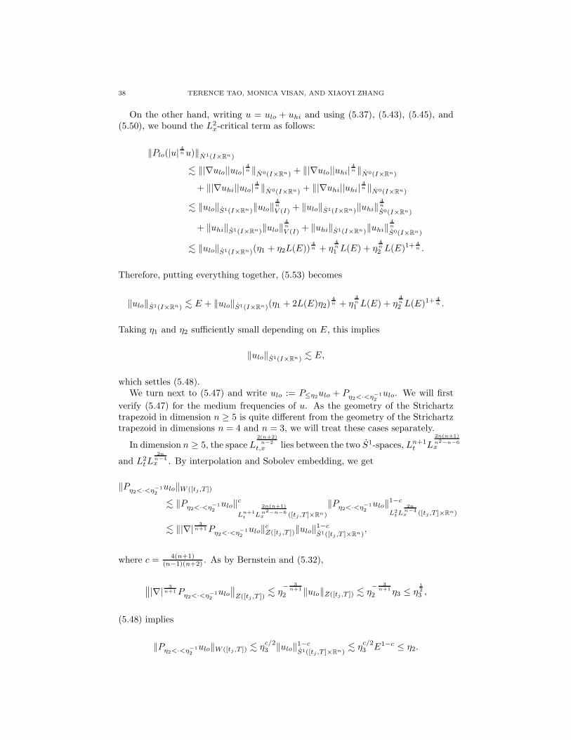
38 TERENCE TAO, MONICA VISAN, AND XIAOYI ZHANG
On the other hand, writing u = ulo + uhi and using (5.37), (5.43), (5.45), and(5.50), we bound the L2
x-critical term as follows:
‖Plo(|u|4n u)‖N1(I×Rn)
. ‖|∇ulo||ulo|4n ‖N0(I×Rn) + ‖|∇ulo||uhi|
4n ‖N0(I×Rn)
+ ‖|∇uhi||ulo|4n ‖N0(I×Rn) + ‖|∇uhi||uhi|
4n ‖N0(I×Rn)
. ‖ulo‖S1(I×Rn)‖ulo‖4n
V (I) + ‖ulo‖S1(I×Rn)‖uhi‖4n
S0(I×Rn)
+ ‖uhi‖S1(I×Rn)‖ulo‖4n
V (I) + ‖uhi‖S1(I×Rn)‖uhi‖4n
S0(I×Rn)
. ‖ulo‖S1(I×Rn)(η1 + η2L(E))4n + η
4n
1 L(E) + η4n
2 L(E)1+4n .
Therefore, putting everything together, (5.53) becomes
‖ulo‖S1(I×Rn) . E + ‖ulo‖S1(I×Rn)(η1 + 2L(E)η2)4n + η
4n
1 L(E) + η4n
2 L(E)1+4n .
Taking η1 and η2 sufficiently small depending on E, this implies
‖ulo‖S1(I×Rn) . E,
which settles (5.48).We turn next to (5.47) and write ulo := P≤η2ulo + Pη2<·<η−1
2ulo. We will first
verify (5.47) for the medium frequencies of u. As the geometry of the Strichartztrapezoid in dimension n ≥ 5 is quite different from the geometry of the Strichartztrapezoid in dimensions n = 4 and n = 3, we will treat these cases separately.
In dimension n ≥ 5, the space L2(n+2)n−2
t,x lies between the two S1-spaces, Ln+1t L
2n(n+1)
n2−n−6x
and L2tL
2nn−4x . By interpolation and Sobolev embedding, we get
‖Pη2<·<η−12ulo‖W ([tj ,T ])
. ‖Pη2<·<η−12
ulo‖c
Ln+1t L
2n(n+1)
n2−n−6x ([tj,T ]×Rn)
‖Pη2<·<η−12ulo‖
1−c
L2tL
2nn−4x ([tj ,T ]×Rn)
. ‖|∇|3
n+1Pη2<·<η−12
ulo‖cZ([tj ,T ])‖ulo‖
1−c
S1([tj ,T ]×Rn),
where c = 4(n+1)(n−1)(n+2) . As by Bernstein and (5.32),
∥∥|∇|3
n+1Pη2<·<η−12ulo
∥∥Z([tj ,T ])
. η− 3
n+1
2 ‖ulo‖Z([tj,T ]) . η− 3
n+1
2 η3 ≤ η123 ,
(5.48) implies
‖Pη2<·<η−12ulo‖W ([tj ,T ]) . η
c/23 ‖ulo‖
1−c
S1([tj ,T ]×Rn). η
c/23 E1−c ≤ η2.
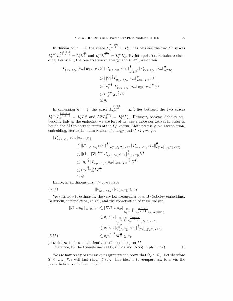
NLS WITH COMBINED POWER-TYPE NONLINEARITIES 39
In dimension n = 4, the space L2(n+2)n−2
t,x = L6t,x lies between the two S1 spaces
Ln+1t L
2n(n+1)
n2−n−6x = L5
tL203x and L∞
t L2n
n−2x = L∞
t L4x. By interpolation, Sobolev embed-
ding, Bernstein, the conservation of energy, and (5.32), we obtain
‖Pη2<·<η−12ulo‖W ([tj ,T ]) . ‖Pη2<·<η−1
2ulo‖
56
L5tL
203
x
‖Pη2<·<η−12ulo‖
16
L∞t L4
x
. ‖|∇|35Pη2<·<η−1
2ulo‖
56
Z([tj ,T ])E16
.(η− 3
52 ‖Pη2<·<η−1
2ulo‖Z([tj ,T ])
) 56E
16
. (η− 3
52 η3)
56E
16
≤ η2.
In dimension n = 3, the space L2(n+2)n−2
t,x = L10t,x lies between the two spaces
Ln+1t L
2n(n+1)
n2−n−6x = L4
tL∞x and L∞
t L2n
n−2x = L∞
t L6x. However, because Sobolev em-
bedding fails at the endpoint, we are forced to take ε more derivatives in order tobound the L4
tL∞x -norm in terms of the L4
t,x-norm. More precisely, by interpolation,embedding, Bernstein, conservation of energy, and (5.32), we get
‖Pη2<·<η−12
ulo‖W ([tj,T ])
. ‖Pη2<·<η−12ulo‖
25
L4tL
∞x ([tj ,T ])×Rn‖Pη2<·<η−1
2ulo‖
35
L∞t L6
t ([tj ,T ]×Rn)
. ‖(1 + |∇|)34+ǫPη2<·<η−1
2ulo‖
25
Z([tj,T ])E35
.(η− 3
42 ‖Pη2<·<η−1
2ulo‖Z([tj ,T ])
) 25E
35
. (η− 3
42 η3)
25E
35
≤ η2.
Hence, in all dimensions n ≥ 3, we have
‖uη2<·<η−12‖W ([tj ,T ]) ≤ η2.(5.54)
We turn now to estimating the very low frequencies of u. By Sobolev embedding,Bernstein, interpolation, (5.46), and the conservation of mass, we get
‖P≤η2ulo‖W ([tj ,T ]) . ‖∇P≤η2ulo‖L
2(n+2)n−2
t L
2n(n+2)
n2+4x ([tj ,T ]×Rn)
. η2‖ulo‖L
2(n+2)n−2
t L
2n(n+2)
n2+4x ([tj ,T ]×Rn)
. η2‖ulo‖n−2n
V ([tj ,T ])‖ulo‖2n
L∞t L2
x([tj ,T ]×Rn)
. η2ηn−2n
1 M2n ≤ η2,(5.55)
provided η1 is chosen sufficiently small depending on M .Therefore, by the triangle inequality, (5.54) and (5.55) imply (5.47).
We are now ready to resume our argument and prove that Ω2 ⊂ Ω1. Let thereforeT ∈ Ω2. We will first show (5.39). The idea is to compare ulo to v via theperturbation result Lemma 3.6.
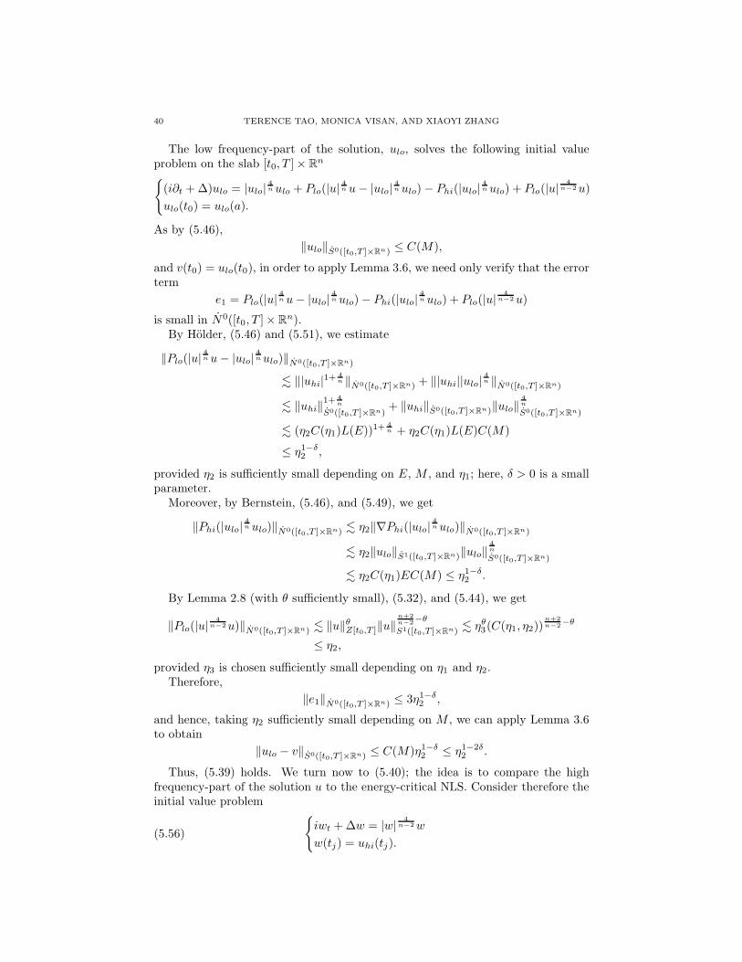
40 TERENCE TAO, MONICA VISAN, AND XIAOYI ZHANG
The low frequency-part of the solution, ulo, solves the following initial valueproblem on the slab [t0, T ]× Rn
(i∂t +∆)ulo = |ulo|
4n ulo + Plo(|u|
4n u− |ulo|
4n ulo)− Phi(|ulo|
4n ulo) + Plo(|u|
4n−2u)
ulo(t0) = ulo(a).
As by (5.46),
‖ulo‖S0([t0,T ]×Rn) ≤ C(M),
and v(t0) = ulo(t0), in order to apply Lemma 3.6, we need only verify that the errorterm
e1 = Plo(|u|4n u− |ulo|
4n ulo)− Phi(|ulo|
4n ulo) + Plo(|u|
4n−2u)
is small in N0([t0, T ]× Rn).By Holder, (5.46) and (5.51), we estimate
‖Plo(|u|4n u− |ulo|
4nulo)‖N0([t0,T ]×Rn)
. ‖|uhi|1+ 4
n ‖N0([t0,T ]×Rn) + ‖|uhi||ulo|4n ‖N0([t0,T ]×Rn)
. ‖uhi‖1+ 4
n
S0([t0,T ]×Rn)+ ‖uhi‖S0([t0,T ]×Rn)‖ulo‖
4n
S0([t0,T ]×Rn)
. (η2C(η1)L(E))1+4n + η2C(η1)L(E)C(M)
≤ η1−δ2 ,
provided η2 is sufficiently small depending on E, M , and η1; here, δ > 0 is a smallparameter.
Moreover, by Bernstein, (5.46), and (5.49), we get
‖Phi(|ulo|4n ulo)‖N0([t0,T ]×Rn) . η2‖∇Phi(|ulo|
4nulo)‖N0([t0,T ]×Rn)
. η2‖ulo‖S1([t0,T ]×Rn)‖ulo‖4n
S0([t0,T ]×Rn)
. η2C(η1)EC(M) ≤ η1−δ2 .
By Lemma 2.8 (with θ sufficiently small), (5.32), and (5.44), we get
‖Plo(|u|4
n−2u)‖N0([t0,T ]×Rn) . ‖u‖θZ[t0,T ]‖u‖n+2n−2−θ
S1([t0,T ]×Rn) . ηθ3(C(η1, η2))n+2n−2−θ
≤ η2,
provided η3 is chosen sufficiently small depending on η1 and η2.Therefore,
‖e1‖N0([t0,T ]×Rn) ≤ 3η1−δ2 ,
and hence, taking η2 sufficiently small depending on M , we can apply Lemma 3.6to obtain
‖ulo − v‖S0([t0,T ]×Rn) ≤ C(M)η1−δ2 ≤ η1−2δ
2 .
Thus, (5.39) holds. We turn now to (5.40); the idea is to compare the highfrequency-part of the solution u to the energy-critical NLS. Consider therefore theinitial value problem
(5.56)
iwt +∆w = |w|
4n−2w
w(tj) = uhi(tj).
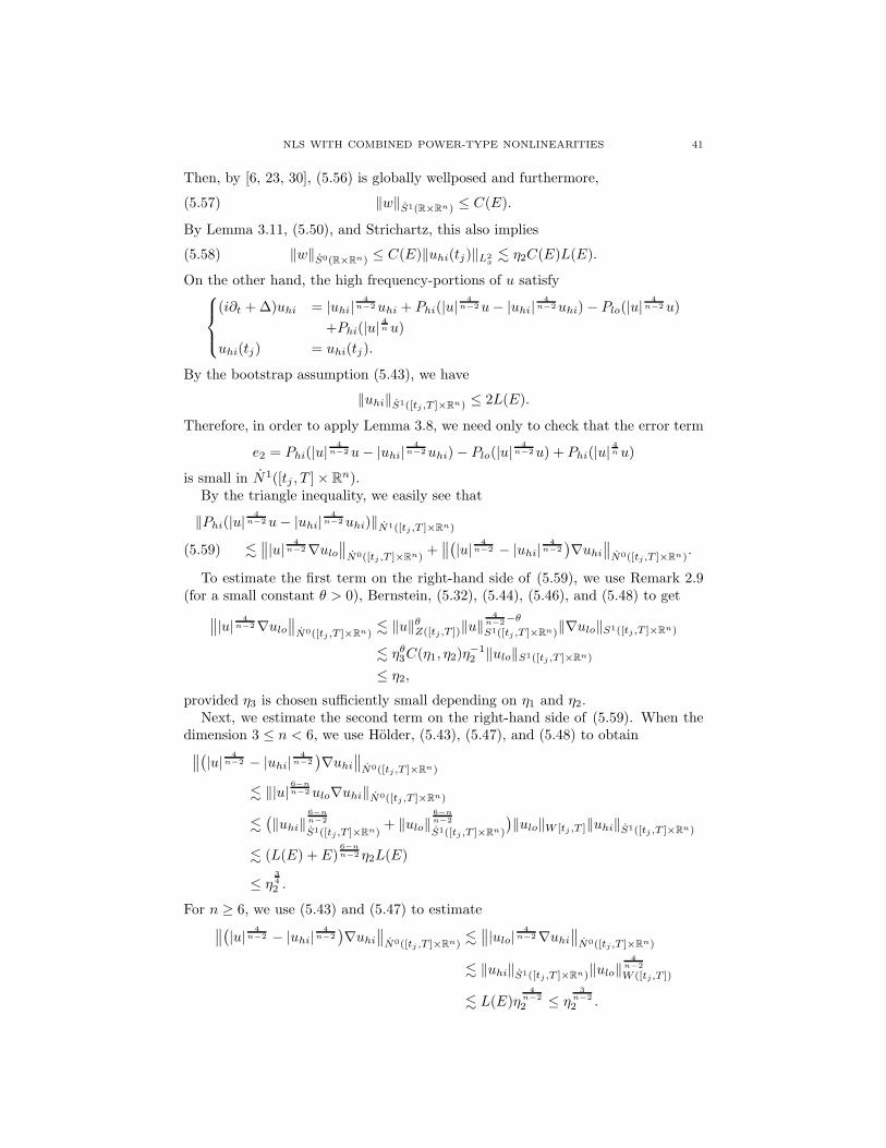
NLS WITH COMBINED POWER-TYPE NONLINEARITIES 41
Then, by [6, 23, 30], (5.56) is globally wellposed and furthermore,
‖w‖S1(R×Rn) ≤ C(E).(5.57)
By Lemma 3.11, (5.50), and Strichartz, this also implies
‖w‖S0(R×Rn) ≤ C(E)‖uhi(tj)‖L2x. η2C(E)L(E).(5.58)
On the other hand, the high frequency-portions of u satisfy
(i∂t +∆)uhi = |uhi|4
n−2uhi + Phi(|u|4
n−2u− |uhi|4
n−2uhi)− Plo(|u|4
n−2u)
+Phi(|u|4n u)
uhi(tj) = uhi(tj).
By the bootstrap assumption (5.43), we have
‖uhi‖S1([tj ,T ]×Rn) ≤ 2L(E).
Therefore, in order to apply Lemma 3.8, we need only to check that the error term
e2 = Phi(|u|4
n−2u− |uhi|4
n−2uhi)− Plo(|u|4
n−2u) + Phi(|u|4n u)
is small in N1([tj , T ]× Rn).By the triangle inequality, we easily see that
‖Phi(|u|4
n−2u− |uhi|4
n−2uhi)‖N1([tj ,T ]×Rn)
.∥∥|u| 4
n−2∇ulo
∥∥N0([tj ,T ]×Rn)
+∥∥(|u| 4
n−2 − |uhi|4
n−2)∇uhi
∥∥N0([tj,T ]×Rn)
.(5.59)
To estimate the first term on the right-hand side of (5.59), we use Remark 2.9(for a small constant θ > 0), Bernstein, (5.32), (5.44), (5.46), and (5.48) to get
∥∥|u| 4n−2∇ulo
∥∥N0([tj ,T ]×Rn)
. ‖u‖θZ([tj,T ])‖u‖4
n−2−θ
S1([tj ,T ]×Rn)‖∇ulo‖S1([tj ,T ]×Rn)
. ηθ3C(η1, η2)η−12 ‖ulo‖S1([tj ,T ]×Rn)
≤ η2,
provided η3 is chosen sufficiently small depending on η1 and η2.Next, we estimate the second term on the right-hand side of (5.59). When the
dimension 3 ≤ n < 6, we use Holder, (5.43), (5.47), and (5.48) to obtain∥∥(|u| 4
n−2 − |uhi|4
n−2
)∇uhi
∥∥N0([tj,T ]×Rn)
. ‖|u|6−nn−2ulo∇uhi‖N0([tj ,T ]×Rn)
.(‖uhi‖
6−nn−2
S1([tj ,T ]×Rn)+ ‖ulo‖
6−nn−2
S1([tj ,T ]×Rn)
)‖ulo‖W [tj ,T ]‖uhi‖S1([tj ,T ]×Rn)
. (L(E) + E)6−nn−2 η2L(E)
≤ η342 .
For n ≥ 6, we use (5.43) and (5.47) to estimate∥∥(|u| 4
n−2 − |uhi|4
n−2
)∇uhi
∥∥N0([tj ,T ]×Rn)
.∥∥|ulo|
4n−2∇uhi
∥∥N0([tj ,T ]×Rn)
. ‖uhi‖S1([tj ,T ]×Rn)‖ulo‖4
n−2
W ([tj,T ])
. L(E)η4
n−2
2 ≤ η3
n−2
2 .
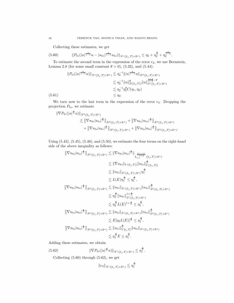
42 TERENCE TAO, MONICA VISAN, AND XIAOYI ZHANG
Collecting these estimates, we get
‖Phi(|u|4
n−2u− |uhi|4
n−2uhi)‖N1([tj ,T ]×Rn) ≤ η2 + η342 + η
3n−2
2 .(5.60)
To estimate the second term in the expression of the error e2, we use Bernstein,Lemma 2.8 (for some small constant θ > 0), (5.32), and (5.44):
‖Plo(|u|4
n−2u)‖N1([tj ,T ]×Rn) . η−12 ‖|u|
4n−2u‖N0([tj ,T ]×Rn)
. η−12 ‖u‖θZ([tj,T ])‖u‖
n+2n−2−θ
S1([tj ,T ]×Rn)
. η−12 ηθ3C(η1, η2)
≤ η2.(5.61)
We turn now to the last term in the expression of the error e2. Dropping theprojection Phi, we estimate
‖∇Phi(|u|4n u)‖N0([tj ,T ]×Rn)
.∥∥∇uhi|ulo|
4n
∥∥N0([tj,T ]×Rn)
+∥∥∇uhi|uhi|
4n
∥∥N0([tj ,T ]×Rn)
+∥∥∇ulo|uhi|
4n
∥∥N0([tj ,T ]×Rn)
+∥∥∇ulo|ulo|
4n
∥∥N0([tj ,T ]×Rn)
.
Using (5.43), (5.45), (5.48), and (5.50), we estimate the four terms on the right-handside of the above inequality as follows:
∥∥∇uhi|ulo|4n
∥∥N0([tj ,T ]×Rn)
. ‖∇uhi|ulo|4n ‖
L
2(n+2)n+4
t,x ([tj ,T ]×Rn)
. ‖∇uhi‖V ([tj ,T ])‖ulo‖4n
V ([tj ,T ])
. ‖uhi‖S1([tj ,T ]×Rn)η4n
1
. L(E)η4n
1 ≤ η3n
1 ,∥∥∇uhi|uhi|
4n
∥∥N0([tj ,T ]×Rn)
. ‖uhi‖S1([tj ,T ]×Rn)‖uhi‖4n
S0([tj,T ]×Rn)
. η4n
2 ‖uhi‖1+ 4
n
S1([tj ,T ]×Rn)
. η4n
2 L(E)1+4n ≤ η
3n
1 ,∥∥∇ulo|uhi|
4n
∥∥N0([tj ,T ]×Rn)
. ‖ulo‖S1([tj ,T ]×Rn)‖uhi‖4n
S0([tj ,T ]×Rn)
. E[η2L(E)]4n ≤ η
3n
1 ,∥∥∇ulo|ulo|
4n
∥∥N0([tj ,T ]×Rn)
. ‖ulo‖4n
V [tj ,T ]‖ulo‖S1([tj ,T ]×Rn)
. η4n
1 E ≤ η3n
1 .
Adding these estimates, we obtain
‖∇Phi(|u|4n u)‖N1([tj ,T ]×Rn) . η
3n
1 .(5.62)
Collecting (5.60) through (5.62), we get
‖e2‖N1([tj ,T ]×Rn) . η3n
1
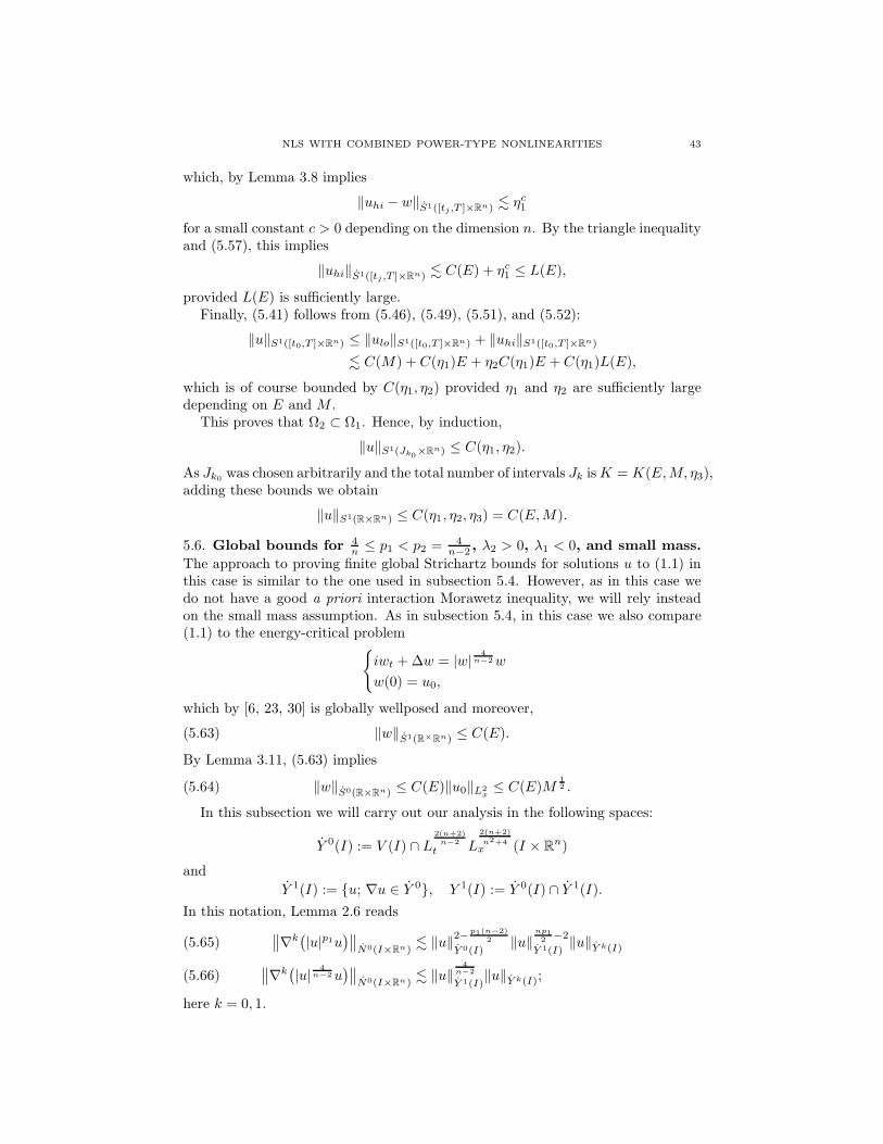
NLS WITH COMBINED POWER-TYPE NONLINEARITIES 43
which, by Lemma 3.8 implies
‖uhi − w‖S1([tj,T ]×Rn) . ηc1
for a small constant c > 0 depending on the dimension n. By the triangle inequalityand (5.57), this implies
‖uhi‖S1([tj ,T ]×Rn) . C(E) + ηc1 ≤ L(E),
provided L(E) is sufficiently large.Finally, (5.41) follows from (5.46), (5.49), (5.51), and (5.52):
‖u‖S1([t0,T ]×Rn) ≤ ‖ulo‖S1([t0,T ]×Rn) + ‖uhi‖S1([t0,T ]×Rn)
. C(M) + C(η1)E + η2C(η1)E + C(η1)L(E),
which is of course bounded by C(η1, η2) provided η1 and η2 are sufficiently largedepending on E and M .
This proves that Ω2 ⊂ Ω1. Hence, by induction,
‖u‖S1(Jk0×Rn) ≤ C(η1, η2).
As Jk0 was chosen arbitrarily and the total number of intervals Jk isK = K(E,M, η3),adding these bounds we obtain
‖u‖S1(R×Rn) ≤ C(η1, η2, η3) = C(E,M).
5.6. Global bounds for 4n ≤ p1 < p2 = 4
n−2 , λ2 > 0, λ1 < 0, and small mass.
The approach to proving finite global Strichartz bounds for solutions u to (1.1) inthis case is similar to the one used in subsection 5.4. However, as in this case wedo not have a good a priori interaction Morawetz inequality, we will rely insteadon the small mass assumption. As in subsection 5.4, in this case we also compare(1.1) to the energy-critical problem
iwt +∆w = |w|
4n−2w
w(0) = u0,
which by [6, 23, 30] is globally wellposed and moreover,
‖w‖S1(R×Rn) ≤ C(E).(5.63)
By Lemma 3.11, (5.63) implies
‖w‖S0(R×Rn) ≤ C(E)‖u0‖L2x≤ C(E)M
12 .(5.64)
In this subsection we will carry out our analysis in the following spaces:
Y 0(I) := V (I) ∩ L2(n+2)n−2
t L2(n+2)
n2+4x (I × R
n)
and
Y 1(I) := u; ∇u ∈ Y 0, Y 1(I) := Y 0(I) ∩ Y 1(I).
In this notation, Lemma 2.6 reads
∥∥∇k(|u|p1u
)∥∥N0(I×Rn)
. ‖u‖2−p1(n−2)
2
Y 0(I)‖u‖
np12 −2
Y 1(I)‖u‖Y k(I)(5.65)
∥∥∇k(|u|
4n−2u
)∥∥N0(I×Rn)
. ‖u‖4
n−2
Y 1(I)‖u‖Y k(I);(5.66)
here k = 0, 1.
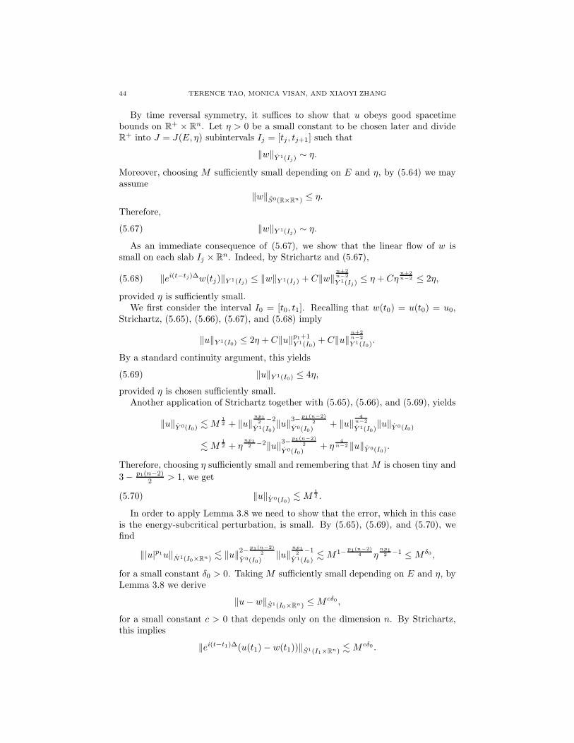
44 TERENCE TAO, MONICA VISAN, AND XIAOYI ZHANG
By time reversal symmetry, it suffices to show that u obeys good spacetimebounds on R+ × Rn. Let η > 0 be a small constant to be chosen later and divideR+ into J = J(E, η) subintervals Ij = [tj , tj+1] such that
‖w‖Y 1(Ij)∼ η.
Moreover, choosing M sufficiently small depending on E and η, by (5.64) we mayassume
‖w‖S0(R×Rn) ≤ η.
Therefore,
‖w‖Y 1(Ij) ∼ η.(5.67)
As an immediate consequence of (5.67), we show that the linear flow of w issmall on each slab Ij × Rn. Indeed, by Strichartz and (5.67),
‖ei(t−tj)∆w(tj)‖Y 1(Ij) ≤ ‖w‖Y 1(Ij) + C‖w‖n+2n−2
Y 1(Ij)≤ η + Cη
n+2n−2 ≤ 2η,(5.68)
provided η is sufficiently small.We first consider the interval I0 = [t0, t1]. Recalling that w(t0) = u(t0) = u0,
Strichartz, (5.65), (5.66), (5.67), and (5.68) imply
‖u‖Y 1(I0) ≤ 2η + C‖u‖p1+1Y 1(I0)
+ C‖u‖n+2n−2
Y 1(I0).
By a standard continuity argument, this yields
‖u‖Y 1(I0) ≤ 4η,(5.69)
provided η is chosen sufficiently small.Another application of Strichartz together with (5.65), (5.66), and (5.69), yields
‖u‖Y 0(I0). M
12 + ‖u‖
np12 −2
Y 1(I0)‖u‖
3−p1(n−2)2
Y 0(I0)+ ‖u‖
4n−2
Y 1(I0)‖u‖Y 0(I0)
. M12 + η
np12 −2‖u‖
3−p1(n−2)
2
Y 0(I0)+ η
4n−2 ‖u‖Y 0(I0)
.
Therefore, choosing η sufficiently small and remembering that M is chosen tiny and
3− p1(n−2)2 > 1, we get
‖u‖Y 0(I0). M
12 .(5.70)
In order to apply Lemma 3.8 we need to show that the error, which in this caseis the energy-subcritical perturbation, is small. By (5.65), (5.69), and (5.70), wefind
‖|u|p1u‖N1(I0×Rn) . ‖u‖2−p1(n−2)
2
Y 0(I0)‖u‖
np12 −1
Y 1(I0). M1−p1(n−2)
4 ηnp12 −1 ≤ M δ0 ,
for a small constant δ0 > 0. Taking M sufficiently small depending on E and η, byLemma 3.8 we derive
‖u− w‖S1(I0×Rn) ≤ M cδ0 ,
for a small constant c > 0 that depends only on the dimension n. By Strichartz,this implies
‖ei(t−t1)∆(u(t1)− w(t1))‖S1(I1×Rn) . M cδ0 .
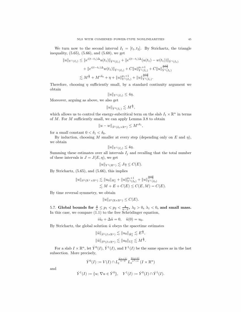
NLS WITH COMBINED POWER-TYPE NONLINEARITIES 45
We turn now to the second interval I1 = [t1, t2]. By Strichartz, the triangleinequality, (5.65), (5.66), and (5.68), we get
‖u‖Y 1(I1) ≤ ‖ei(t−t1)∆u(t1)‖Y 0(I1)+ ‖ei(t−t1)∆(u(t1)− w(t1))‖Y 1(I1)
+ ‖ei(t−t1)∆w(t1)‖Y 1(I1)+ C‖u‖p1+1
Y 1(I1)+ C‖u‖
n+2n−2
Y 1(I1)
. M12 +M cδ0 + η + ‖u‖p1+1
Y 1(I1)+ ‖u‖
n+2n−2
Y 1(I1).
Therefore, choosing η sufficiently small, by a standard continuity argument weobtain
‖u‖Y 1(I1) ≤ 4η.
Moreover, arguing as above, we also get
‖u‖Y 0(I1). M
12 ,
which allows us to control the energy-subcritical term on the slab I1 ×Rn in termsof M . For M sufficiently small, we can apply Lemma 3.8 to obtain
‖u− w‖S1(I0×Rn) ≤ M cδ1 ,
for a small constant 0 < δ1 < δ0.By induction, choosing M smaller at every step (depending only on E and η),
we obtain
‖u‖Y 1(Ij) ≤ 4η.
Summing these estimates over all intervals Ij and recalling that the total numberof these intervals is J = J(E, η), we get
‖u‖Y 1(R+) . Jη ≤ C(E).
By Strichartz, (5.65), and (5.66), this implies
‖u‖S1(R+×Rn) . ‖u0‖H1x+ ‖u‖p1+1
Y 1(I0)+ ‖u‖
n+2n−2
Y 1(I0)
. M + E + C(E) ≤ C(E,M) = C(E).
By time reversal symmetry, we obtain
‖u‖S1(R×Rn) ≤ C(E).
5.7. Global bounds for 4n ≤ p1 < p2 < 4
n−2 , λ2 > 0, λ1 < 0, and small mass.
In this case, we compare (1.1) to the free Schrodinger equation,
iut +∆u = 0, u(0) = u0.
By Strichartz, the global solution u obeys the spacetime estimates
‖u‖S1(I×Rn) . ‖u0‖H1x. E
12 ,
‖u‖S0(I×Rn) . ‖u0‖L2x. M
12 .
For a slab I × Rn, let Y 0(I), Y 1(I), and Y 1(I) be the same spaces as in the lastsubsection. More precisely,
Y 0(I) := V (I) ∩ L2(n+2)n−2
t L2(n+2)
n2+4x (I × R
n)
and
Y 1(I) := u; ∇u ∈ Y 0, Y 1(I) := Y 0(I) ∩ Y 1(I).
46 TERENCE TAO, MONICA VISAN, AND XIAOYI ZHANG
We divide R+ into J = J(E, η) subintervals Ij such that on each Ij = [tj , tj+1],
‖u‖Y 1(Ij)∼ η,
where η > 0 is a small parameter. Choosing M small enough depending on η, wemay assume that on each slab Ij × Rn, we have
‖u‖Y 1(Ij) ∼ η.
We will prove that u obeys good spacetime bounds on each slab Ij×Rn. Considerthe first interval, I0 = [t0, t1]. As u(t0) = u(t0) = u0, by Strichartz and Lemma 2.6,
‖u‖Y 1(I0) ≤ ‖u‖Y 1(I0) + C(λ1, λ2)∑
i=1,2
‖u‖pi+1Y 1(I0)
≤ η + C(λ1, λ2)∑
i=1,2
‖u‖pi+1Y 1(I0)
.
A standard continuity argument yields
‖u‖Y 1(I0) ≤ 2η,
provided η is chosen sufficiently small. Hence, another application of Strichartz andLemma 2.6 implies
‖u‖Y 0(I0). M
12 + C(λ1, λ2)
∑
i=1,2
‖|u|piu‖N0(I0×Rn)
. M12 + C(λ1, λ2)
∑
i=1,2
‖u‖3−pi(n−2)
2
Y 0(I0)‖u‖
npi2 −2
Y 1(I0)
. M12 + C(λ1, λ2)
∑
i=1,2
‖u‖3−pi(n−2)
2
Y 0(I0)η
npi2 −2.
Therefore,
‖u‖Y 0(I0). M
12 ,(5.71)
provided M is chosen sufficiently small.By Strichartz and (5.71), we can now compute the difference between u and u
on the slab I0 × Rn:
‖u− u‖S1(I0×Rn) . C(λ1, λ2)∑
i=1,2
‖u‖2−pi(n−2)
2
Y 0(I0)‖u‖
npi2 −1
Y 1(I0)
. M δ∑
i=1,2
ηnpi2 −1
≤ M δ,
where δ > 0 is a small constant, provided η is chosen sufficiently small. ByStrichartz, this implies
‖ei(t−t1)∆(u(t1)− u(t1))‖S1(I1×Rn) . M δ.(5.72)
We turn now to the second interval, I1 = [t1, t2]. By Strichartz, the triangleinequality, Lemma 2.6, and (5.72), we get
‖u‖Y 1(I1) ≤ ‖ei(t−t1)∆u(t1)‖Y 0(I1)+ ‖ei(t−t1)∆u(t1)‖Y 1(I1)
+ ‖ei(t−t1)∆(u(t1)− u(t1))‖Y 1(I1)+ C(λ1, λ2)
∑
i=1,2
‖u‖pi+1Y 1(I1)
. M12 + η +M δ + C(λ1, λ2)
∑
i=1,2
‖u‖pi+1Y 1(I1)
.
NLS WITH COMBINED POWER-TYPE NONLINEARITIES 47
Another continuity argument yields
‖u‖Y 1(I1) ≤ 2η,(5.73)
provided η and M are chosen sufficiently small. By the same arguments as thoseused to establish (5.71), this implies
‖u‖Y 0(I1). M
12 .(5.74)
Therefore, we can now control the difference between u and u on I1 ×Rn. Indeed,by Strichartz, Lemma 2.6, (5.72), (5.73), and (5.74),
‖u− u‖S1(I1×Rn) . ‖ei(t−t1)∆(u(t1)− u(t1))‖S1(I1×Rn)
+ ‖λ1|u|p1u+ λ2|u|
p2u‖N1(I1×Rn)
. M δ + C(λ1, λ2)∑
i=1,2
‖u‖2−pi(n−2)
2
Y 0(I1)‖u‖
npi2 −1
Y 1(I1)
. M δ + C(λ1, λ2)∑
i=1,2
M1−pi(n−2)
4 ηnpi2 −1
. M δ,
provided δ > 0 is chosen sufficiently small. By Strichartz, this immediately implies
‖ei(t−t2)∆(u(t2)− u(t2))‖Y 1(I2). M δ
and hence one can repeat the argument on the next slab, that is, I2 × Rn. Byinduction, on every slab Ij × Rn, we get
‖u‖Y 1(Ij) ≤ 2η.
Adding these estimates over all intervals Ij and recalling that the total number ofthese intervals is J = J(E, η), we get
‖u‖Y 1(R+) ≤ C(E).
Strichartz estimates and time reversal symmetry (see the end of subsection 5.6)yield the global spacetime bound
‖u‖S1(R×Rn) ≤ C(E).
5.8. Finite global Strichartz norms imply scattering. In this subsection weshow that finite global Strichartz norms imply scattering. As the techniques areclassical, we will only present the construction of the scattering states u± and showthat their linear flow approximates well the solution as t → ±∞ in H1
x. Standardarguments can also be employed to construct the wave operators; for details see,for example, [5].
For simplicity, we will only construct the scattering state in the positive timedirection. Similar arguments can be used to construct the scattering state in thenegative time direction.
For 0 < t < ∞, we define
u+(t) = u0 − i
∫ t
0
e−is∆(λ1|u|p1u+ λ2|u|
p2u)(s)ds.
48 TERENCE TAO, MONICA VISAN, AND XIAOYI ZHANG
As u ∈ S1(R × Rn), Strichartz estimates and Lemma 2.6 imply that u+(t) ∈ H1x
for all t ∈ R+. We will show that u+(t) converges in H1x as t → ∞. Indeed, for
0 < τ < t, we have
‖u+(t)− u+(τ)‖H1x=
∥∥∥∫ t
τ
e−is∆(λ1|u|p1u+ λ2|u|
p2u)(s)ds∥∥∥H1
x
.∥∥∥∫ t
τ
ei(t−s)∆(λ1|u|p1u+ λ2|u|
p2u)(s)ds∥∥∥L∞
t H1x([τ,t]×Rn)
,
which by Strichartz and (2.9) implies
‖u+(t)− u+(τ)‖H1x. C(λ1, λ2)
∑
i=1,2
‖u‖2−pi(n−2)
2
V ([τ,t]) ‖u‖npi2 −2
W ([τ,t])‖(1 + |∇|)u‖V ([τ,t]).
As
‖u‖S1(R×Rn) < ∞,(5.75)
we see that for ε > 0 there exists Tε > 0 such that
‖u+(t)− u+(τ)‖H1x≤ ε
for any t, τ > Tε. Thus, u+(t) converges in H1x as t → ∞ to some function u+.
Moreover, Strichartz and (2.9) imply that
u+ := u0 − i
∫ ∞
0
e−is∆(λ1|u|p1u+ λ2|u|
p2u)(s)ds.
Next, we show that the linear evolution eit∆u+ approximates u(t) in H1x as
t → ∞. Indeed, by Strichartz and Lemma 2.6,
‖e−it∆u(t)− u+‖H1x=
∥∥∥∫ ∞
t
e−is∆(λ1|u|p1u+ λ2|u|
p2u)(s)ds∥∥∥H1
x
=∥∥∥∫ ∞
t
ei(t−s)∆(λ1|u|p1u+ λ2|u|
p2u)(s)ds∥∥∥H1
x
.∑
i=1,2
‖u‖2−pi(n−2)
2
V ([t,∞)) ‖u‖npi2 −2
W ([t,∞))‖(1 + |∇|)u‖V ([t,∞)),
which obviously tends to 0 as t → ∞ (see (5.75)).
6. Finite time blowup
To prove blowup under the assumptions on the nonlinearities described in The-orem 1.5, we will follow the convexity method of Glassey, [8]. More precisely, wewill consider the variance
V (t) =
∫
Rn
|x|2|u(t, x)|2dx
and show that as a function of t > 0, it is decreasing and concave, which suggeststhe existence of a blowup time T∗ at which V (T∗) = 0.
For strong H1x-solutions u to (1.1) with initial data u0 ∈ Σ, it is known that
V ∈ C2(−Tmin, Tmax); see, for example, [5]. Formal computations (which aremade rigorous in [5]) prove
NLS WITH COMBINED POWER-TYPE NONLINEARITIES 49
Lemma 6.1. For all t ∈ (−Tmin, Tmax), we have
V ′(t) = −4y(t),(6.1)
where
y(t) = −Im
∫
Rn
ruur(t)dx.
Moreover,
V ′′(t) = −4y′(t) = 8‖∇u(t)‖22 +4nλ1p1
p1+2 ‖u(t)‖p1+2p1+2 +
4nλ2p2
p2+2 ‖u(t)‖p2+2p2+2.(6.2)
In what follows, we will show that the first and second derivatives of the varianceare negative for positive times t. More precisely, in each of the three cases describedin Theorem 1.5, we will show that
(6.3) y′(t) ≥ c‖∇u(t)‖22 > 0
for a small positive constant c. Thus, by (6.2) it follows that V ′′(t) < 0 for all timest ∈ (−Tmin, Tmax), which implies that V (t) is concave. Moreover, as by hypothesis
y(0) = y0 > 0,
(6.3) implies that y(t) > y(0) > 0, for all times t > 0. By (6.1), this yields V ′(t) < 0for positive times t and hence, V (t) is decreasing for t > 0.
Alternatively, by Holder, for all times t ∈ (−Tmin, Tmax),
y(t) ≤ ‖xu(t)‖2‖∇u(t)‖2
and hence,
(6.4) ‖∇u(t)‖2 ≥y(t)
‖xu0‖2.
By (6.3) and (6.4), we derive a first order ODE for y,
(6.5)
y′(t) ≥ c y2(t)
‖xu0‖22
y(0) = y0 > 0,
which implies that there exists 0 < T∗ ≤ ‖xu0‖22
cy0such that
limt→T∗
‖∇u(t)‖2 = ∞.
For the remainder of the section, we will derive (6.3) in each of the three casesdescribed in Theorem 1.5.
Case 1): λ1 > 0 , 0 < p1 < p2, and E < 0.By (6.2), the conservation of energy, and our assumptions, we get
y′(t) = −2‖∇u(t)‖22 + p2n
12‖∇u(t)‖22 +
λ1
p1+2‖u(t)‖p1+2p1+2 − E
− nλ1p1
p1+2 ‖u(t)‖p1+2p1+2
= p2n−42 ‖∇u(t)‖22 +
p2nλ1
p1+2 − p1nλ1
p1+2
‖u(t)‖p1+2
p1+2 − p2nE
≥ p2n−42 ‖∇u(t)‖22 +
nλ1(p2−p1)p1+2 ‖u(t)‖p1+2
p1+2
≥ p2n−42 ‖∇u(t)‖22,
and hence (6.3) holds with c := p2n−42 .
50 TERENCE TAO, MONICA VISAN, AND XIAOYI ZHANG
Case 2): λ1 < 0, 4n < p1 < p2, and E < 0.
In this case, by (6.2) and the conservation of energy, we obtain
y′(t) = −2‖∇u(t)‖22 + p1n
12‖∇u(t)‖22 +
λ2
p2+2‖u(t)‖p2+2p2+2 − E
− p2nλ2
p2+2 ‖u(t)‖p2+2p2+2
= p1n−42 ‖∇u(t)‖22 +
nλ2(p1−p2)p2+2 ‖u(t)‖p2+2
p2+2 − p1nE
≥ p1n−42 ‖∇u(t)‖22,
which implies (6.3) with c := p1n−42 .
Case 3): λ1 < 0, 0 < p1 ≤ 4n , and E + CM < 0 for some constant C =
C(λ1, λ2, p1, p2, n) to be specified momentarily.The idea is to use part of the contribution coming from the higher power nonlin-
earity to obtain a positive multiple of the kinetic energy and the rest to annihilatethe effect of the resulting lower power term. The details are as follows.
As p2 > 4n , we can find a small constant ε such that p2 > 2(2+ε)
n . It is immediate
that θ := 2(2+ε)p2n
< 1. Therefore, from the conservation of energy, we get
y′(t) = −2‖∇u(t)‖22 −nλ2p2θp2+2 ‖u(t)‖p2+2
p2+2 −nλ2p2(1−θ)
p2+2 ‖u(t)‖p2+2p2+2 −
nλ1p1
p1+2 ‖u‖p1+2p1+2
≥ −2‖∇u(t)‖22 + p2nθ
12‖∇u(t)‖22 +
λ1
p1+2‖u(t)‖p1+2p1+2 − E
− nλ2p2(1−θ)p2+2 ‖u(t)‖p2+2
p2+2 −nλ1p1θp1+2 ‖u(t)‖p1+2
p1+2
≥−2 + p2nθ
2
‖∇u(t)‖22 +
nλ1θ(p2−p1)p1+2 ‖u(t)‖p1+2
p1+2 − p2nθE
− nλ2p2(1−θ)p2+2 ‖u(t)‖p2+2
p2+2
= ε‖∇u(t)‖22 +nλ1θ(p2−p1)
p1+2 ‖u(t)‖p1+2p1+2 −
nλ2p2(1−θ)p2+2 ‖u(t)‖p2+2
p2+2 − p2nθE.
By Young’s inequality, for any positive constants a and δ,
ap1+2 ≤ C(δ)a2 + δap2+2.
Hence,
n|λ1|θ(p2−p1)p1+2 ‖u(t)‖p1+2
p1+2 ≤ C(δ)n|λ1|θ(p2−p1)p1+2 ‖u(t)‖22 + δ nθ|λ1|(p2−p1)
p1+2 ‖u(t)‖p2+2p2+2.
Choosing δ > 0 sufficiently small such that
δnθ|λ1|(p2 − p1)
p1 + 2<
np2|λ2|(1− θ)
p2 + 2,
we obtain
y′(t) ≥ ε‖∇u(t)‖22 − C(λ1, λ2, p1, p2, n)M − p2nθE,
which, as long as
p2nθE + C(λ1, λ2, p1, p2, n)M < 0,
yields
y′(t) ≥ ε‖∇u(t)‖22.
This proves (6.3) in this case.Hence, (6.3) holds in all three cases described in Theorem 1.5, which implies for
the reasons given above the existence of a time T∗ ≤ ‖xu0‖22
y0such that
limt→T∗
‖∇u(t)‖2 = ∞.
NLS WITH COMBINED POWER-TYPE NONLINEARITIES 51
7. Scattering in Σ
In this section we prove Theorem 1.8. When α(n) < p1 < p2 < 4n−2 , the result
is well-known (see [28, 11, 5]) and we will not revisit the proof here. Instead, wewill present the proof of Theorem 1.8 in the case α(n) < p1 < p2 = 4
n−2 , which isnot covered by these earlier results.
As both nonlinearities are assumed defocusing, without loss of generality we mayassume λ1 = λ2 = 1. We will also write p instead of p1 to ease notation. Notethat under our assumptions, Theorem 1.1 implies the existence of a unique globalsolution u. Moreover, on every slab I × Rn u obeys the following estimate:
‖u‖S1(I×Rn) ≤ C(‖u0‖H1x, |I|).(7.1)
Next, we introduce the Galilean operator associated with the linear Schrodingeroperator i∂t +∆,
H(t) := x+ 2it∇.
Note that we can also write
H(t) = 2itei|x|2
4 t∇(e−i|x|2
4 t·) = eit∆xe−it∆.(7.2)
From the first identity in (7.2) we see that H(t) behaves morally like a deriva-
tive when applied to the Hamiltonian nonlinearity F (u) = |u|pu + |u|4
n−2u, whichcommutes with phase rotations. More precisely, we have
H(t)F (u) = ∂zF (u)H(t)u− ∂zF (u)H(t)u.(7.3)
The first step to prove scattering in Σ is to use the local spacetime bound (7.1)
and the fact that xu0 ∈ L2x to derive S0 spacetime bounds on Hu on every slab
I × Rn. By time reversal symmetry, we may assume I = [0, T ]. By (7.1), we cansplit [0, T ] into J = J(‖u0‖H1
x, T, η) subintervals Ij = [tj , tj+1] such that
‖u‖X1(Ij)∼ η,(7.4)
where η > 0 is a small constant to be chosen later. We will derive Strichartz boundson Hu on every slab Ij × Rn.
Fix therefore Ij ; on this interval u satisfies
u(t) = ei(t−tj)∆u(tj)− i
∫ t
tj
ei(t−s)∆(|u|pu+ |u|4
n−2u)(s)ds.
By (7.2), this yields
H(t)u(t) = ei(t−tj)∆H(tj)u(tj)− i
∫ t
tj
ei(t−s)∆H(s)(|u|pu+ |u|4
n−2u)(s)ds,
By Strichartz, Lemma 2.5, (7.3), and (7.4), we estimate
‖Hu‖S0(Ij×Rn) . ‖H(tj)u(tj)‖L2x+ |Ij |
1− p(n−2)4 ‖u‖p
X1(Ij)‖Hu‖S0(Ij×Rn)
+ ‖u‖4
n−2
X1(Ij)‖Hu‖S0(Ij×Rn)
. ‖H(tj)u(tj)‖L2x+ T 1−p(n−2)
4 ηp‖Hu‖S0(Ij×Rn)
+ η4
n−2 ‖Hu‖S0(Ij×Rn),
which implies‖Hu‖S0(Ij×Rn) . ‖H(tj)u(tj)‖L2
x,
52 TERENCE TAO, MONICA VISAN, AND XIAOYI ZHANG
provided η is chosen sufficiently small depending on |I| = T . By induction, for eachj we get
‖Hu‖S0(Ij×Rn) . ‖xu0‖L2x.
Therefore, adding these estimates over all subintervals Ij , we obtain
‖Hu‖S0(I×Rn) ≤ C(‖xu0‖L2x, |I|).(7.5)
In order to prove scattering, rather than a local spacetime bound, one needs toderive global spacetime bounds. To accomplish this, we will use the pseudoconfor-mal identity to prove that the global solution u decays as t → ∞. More precisely,we will show that t 7→ ‖u(t)‖ 2n
n−2and t 7→ ‖u(t)‖p+2 are decreasing.
Introduce the pseudoconformal energy
h(t) := ‖H(t)u(t)‖22 + 8t2(
1p+2‖u(t)‖
p+2p+2 +
n−22n ‖u(t)‖
2nn−22n
n−2
).
A standard computation (see e.g. [24]) shows that
(7.6) h′(t) = t( 4(4−pn)
p+2 ‖u(t)‖p+2p+2 −
16n ‖u(t)‖
2nn−22n
n−2
):= tθ(t).
Again, we can justify this computation in the class Σ (treating h′(t) as a weakderivative of h(t)) by first mollifying u0 and the nonlinearity and then taking limitsat the end using the well-posedness theory; we omit the standard details.
If 4n ≤ p < 4
n−2 , we integrate (7.6) with respect to the time variable over the
compact interval [0, t] to obtain
‖H(t)u(t)‖22 +8t2
p+2‖u(t)‖p+2p+2 +
4(n−2)t2
n ‖u(t)‖2n
n−22n
n−2
(7.7)
= ‖xu0‖22 +
4(4−pn)p+2
∫ t
0
s
∫
Rn
|u(s, x)|p+2dxds− 16n
∫ t
0
s
∫
Rn
|u(s, x)|2n
n−2 dxds.
Thus, in this case,
‖u(t)‖p+2p+2 + ‖u(t)‖
2nn−22n
n−2
. t−2.(7.8)
If 0 < p < 4n , we integrate (7.6) over the compact interval [1, t]; we get
h(t) = h(1) +
∫ t
1
sθ(s)ds, for t ≥ 1.
In particular,
8t2
p+2‖u(t)‖p+2p+2 ≤ h(1) + 4(4−pn)
p+2
∫ t
1
s‖u(s)‖p+2p+2ds,
which by Grownwall’s inequality implies
‖u(t)‖p+2p+2 . t−
pn2 .
Combining this with (7.7), we obtain
h(t) . 1 + t2−pn2
and hence,
‖u(t)‖2n
n−22n
n−2
. t−pn2 , ∀t ≥ 1.
NLS WITH COMBINED POWER-TYPE NONLINEARITIES 53
Thus, for 0 < p < 4n and t ≥ 1 we get
‖u(t)‖p+2p+2 + ‖u(t)‖
2nn−22n
n−2
. t−pn2 .(7.9)
Collecting (7.8) and (7.9), we obtain
‖u(t)‖p+2p+2 + ‖u(t)‖
2nn−22n
n−2
. t−2 + t−pn2(7.10)
for all 0 < p < 4n−2 and t ≥ 1.
Next, we show that the decay estimate (7.10) implies that the Strichartz normsof the solution are small when measured over the slab [T,∞)×Rn for a large enoughtime T . Let δ be such that (δ, p + 2) is a Schrodinger admissible pair. An easycomputation shows that p > α(n) ⇔ 2p > δ − 2. Then, by (7.10), on the slab[T,∞)× Rn with T ≥ 1 we get
‖|u|pu‖Lδ′
t W1,
p+2p+1
x
. ‖u‖LδtW
1,p+2x
‖u‖p
Lδp
δ−2t Lp+2
x
. T−ν‖u‖S1(7.11)
‖|u|4
n−2u‖L2
tW1, 2n
n+2x
. ‖u‖4
n−2
L∞t L
2nn−2x
‖u‖L2
tW1, 2n
n−2x
. T−ν‖u‖S1(7.12)
for some ν > 0. As by (2.3), on [T,∞) u satisfies
u(t) = ei(t−T )∆u(T )− i
∫ ∞
T
ei(t−s)∆(|u|pu+ |u|4
n−2 )u(s)ds,
by Strichartz, (7.11), and (7.12), we get
‖u‖S1([T,∞)×Rn) . ‖u(T )‖H1x+ T−ν‖u‖S1([T,∞)×Rn).
Hence, taking T sufficiently large, by the conservation of energy and mass we obtain
‖u‖S1([T,∞)×Rn) . ‖u(T )‖H1x≤ C(‖u0‖H1
x).(7.13)
Similarly, by Strichartz, (7.2), (7.3), (7.11), and (7.12), we estimate
‖Hu‖S0([T,∞)×Rn) . ‖H(T )u(T )‖L2x+ T−ν‖Hu‖S0([T,∞)×Rn),
which taking T sufficiently large and using (7.5) yields
‖Hu‖S0([T,∞)×Rn) . ‖H(T )u(T )‖L2x≤ C(‖xu0‖L2
x).(7.14)
Combining (7.1) and (7.13), (7.5) and (7.14), and using the time reversal sym-metry, we get
‖u‖S1(R×Rn) ≤ C(‖u0‖H1x)(7.15)
‖Hu‖S0(R×Rn) ≤ C(‖u0‖Σ).(7.16)
Next, we construct the scattering state in the positive time direction. The scat-tering state in the negative time direction is constructed similarly. Let
u+(t) = u0 − i
∫ t
0
e−is∆(|u|pu+ |u|4
n−2u)(s)ds.
We will show that u+(t) is a Cauchy sequence in Σ when t → ∞. Take t1 < t2 < ∞.Then, by Strichartz, (7.2), the fact that eit∆ is unitary on L2
x, (7.11), and (7.12),
54 TERENCE TAO, MONICA VISAN, AND XIAOYI ZHANG
we estimate
‖u+(t1)− u+(t2)‖Σ =∥∥∥∫ t2
t1
e−is∆(|u|pu+ |u|4
n−2u)(s)ds∥∥∥Σ
.∥∥∥∫ t2
t1
e−is∆(|u|pu+ |u|4
n−2u)(s)ds∥∥∥H1
x
+∥∥∥x
∫ t2
t1
e−is∆(|u|pu+ |u|4
n−2u)(s)ds∥∥∥L2
x
.∥∥∥∫ t2
t1
ei(t−s)∆(|u|pu+ |u|4
n−2u)(s)ds∥∥∥H1
x
+∥∥∥∫ t2
t1
ei(t−s)∆H(s)(|u|pu+ |u|4
n−2u)(s)ds∥∥∥L2
x
. t−ν1
(‖u‖S1([t1,t2]×Rn) + ‖Hu‖S0([t1,t2]×Rn)
)
≤ t−ν1 C(‖u0‖Σ).
Therefore, u+(t) is a Cauchy sequence in Σ as t → ∞ and hence, it converges tosome function u+ ∈ Σ. Similar estimates show that
u+ = u0 − i
∫ ∞
0
e−is∆(|u|pu+ |u|4
n−2u)(s)ds.
Finally, we show that u+ is the asymptotic state of e−it∆u(t) as t → ∞. Indeed,similar computations as above yield
‖e−it∆u(t)− u+‖Σ ≤∥∥∥∫ ∞
t
e−is∆(|u|pu+ |u|4
n−2u)(s)ds∥∥∥Σ
. t−ν(‖u‖S1(R×Rn) + ‖Hu‖S0(R×Rn)
)
. t−νC(‖u0‖Σ)
which tends to 0 as t → ∞, as desired.
References
[1] J. Bourgain, Scattering in the energy space and below for 3D NLS, Journal D’Analyse Math-ematique,75 (1998), 267-297.
[2] J. Bourgain, Global well-posedness of defocusing 3D critical NLS in the radial case, JAMS12 (1999), 145–171.
[3] J. Bourgain, New global well-posedness results for non-linear Schrodinger equations, AMSPublications (1999).
[4] T. Cazenave, F.B. Weissler, Critical nonlinear Schrodinger Equation, Non. Anal. TMA 14
(1990), 807–836.[5] T. Cazenave, Semilinear Schrodinger equations, Courant Lecture Notes in Mathematics, 10.
American Mathematical Society, 2003.[6] J. Colliander, M. Keel, G. Staffilani, H. Takaoka, T. Tao, Global well-posedness and scattering
for the energy-critical nonlinear Schrodinger equation in R3, to appear Annals of Math.
[7] J. Colliander, M. Keel, G. Staffilani, H. Takaoka, T. Tao, Existence globale et diffusion pour
l’equation de Schrodinger nonlineaire repulsive cubique sur R3 en dessous l’espace d’energie,
Journees “Equations aux Derivees Partielles” (Forges-les-Eaux, 2002), Exp. No. X, 14, 2002.
[8] R. T. Glassey, On the blowing up of solution to the Cauchy problem for nonlinear Schrodinger
operators, J. Math. Phys. 8 (1977), 1794–1797.[9] J. Ginibre, G. Velo, Scattering theory in the energy space for a class of nonlinear Schrodinger
equations, J. Math. Pure. Appl. 64 (1985), 363–401.
NLS WITH COMBINED POWER-TYPE NONLINEARITIES 55
[10] M. Grillakis, On nonlinear Schrodinger equations., Comm. Partial Differential Equations 25
no. 9-10 (2000), 1827–1844.[11] N. Hayashi, Y. Tsutsumi, Remarks on the scattering problem for nonlinear Schrodinger
equations, Diff. Eq. Math. Phys., (1986), 162–168.[12] T. Kato, On nonlinear Schrodinger equations, Ann. Inst. H. Poincare Phys. Theor. 46 (1987),
113–129.[13] T. Kato, On nonlinear Schrodinger equations, II. Hs-solutions and unconditional well-
posedness, J. d’Analyse. Math. 67, (1995), 281–306.[14] M. Keel, T. Tao, Endpoint Strichartz Estimates, Amer. Math. J. 120 (1998), 955–980.[15] J. Lin, W. Strauss, Decay and scattering of solutions of a nonlinear Schrodinger equation,
Journ. Funct. Anal. 30 (1978), 245–263.[16] F. Merle, Determination of blow-up solutions with minimal mass for nonlinear Schrodinger
equations with critical power, Duke Math. J. 69 (1993), 427–454.[17] F. Merle, P. Raphael, The blow-up dynamic and upper bound on the blow-up rate for critical
nonlinear Schrodinger equation, Ann. of Math. 161 (2005), 157–222.[18] F. Merle, P. Raphael, Profiles and quantization of the blow up mass for critical nonlinear
Schrodinger equation, Comm. Math. Phys. 253 (2005), 675–704.[19] F. Merle, Y. Tsutsumi, L2-concentration of blow-up solutions for the nonlinear Schrodinger
equation with the critical power nonlinearity, J. Diffe. Equa. 84 (1990), 205-214.
[20] C. Morawetz, Time decay for the nonlinear Klein-Gordon equation, Proc. Roy. Soc. A 306
(1968), 291–296.[21] K. Nakanishi, Energy scattering for non-linear Klein-Gordon and Schrodinger equations in
spatial dimensions 1 and 2, JFA 169 (1999), 201–225.[22] K. Nakanishi, Scattering theory for nonlinear Klein-Gordon equation with Sobolev critical
power, IMRN 1 (1999), 31–60.[23] E. Ryckman, M. Visan Global well-posedness and scattering for the defocusing energy-critical
nonlinear Schrodinger equation in R1+4, preprint math.AP/0501462.
[24] C. Sulem, P.-L. Sulem, The nonlinear Schrodinger equation: Self-focusing and wave collapse,Springer-Verlag, New York, (1999), p. 25.
[25] T. Tao, On the asymptotic behavior of large radial data for a focusing non-linear Schrodinger
equation, preprint math.AP/0309428.[26] T. Tao, Global well-posedness and scattering for the higher-dimensional energy-critical non-
linear Schrodinger equation for radial data, New York Journal of Math., 11 (2005), 57-80.[27] T. Tao, M. Visan Stability of energy-critical nonlinear Schrodinger equations in high dimen-
sions, Electron. J. Diff. Eqns., 118 (2005), 1-28.[28] Y. Tsutsumi, Scattering problem for nonlinear Schrodinger equations, Ann. Inst. H. Poincar
Phys. Thor. 43 (1985), 321–347.[29] M. Visan, The defocusing energy-critical nonlinear Schrodinger equation in higher dimen-
sions, preprint math.AP/0508298.[30] M. Visan, The defocusing energy-critical nonlinear Schrodinger equation in dimensions four
and higher, Ph.D. Thesis, UCLA, in preparation.[31] X. Zhang, On Cauchy problem of 3-D energy critical Schrodinger equation with subcritical
perturbations, preprint.
University of California, Los Angeles
University of California, Los Angeles
Academy of Mathematics and System Sciences, Chinese Academy of Sciences


![Nonlinear stability of degenerate shock profilesphoward/papers/degnonlinshort.pdf · nonlinear Schrodinger equation and the Ginzburg–Landau equation [21]. The algebraic (and non-integrable)](https://img.pdfslide.net/doc/110x75/6086050bfe80cf0c283eca7c/nonlinear-stability-of-degenerate-shock-proiles-phowardpapers-nonlinear-schrodinger.jpg)