Embed Size (px)
DESCRIPTION
The Normal Distribution & Standard Normal Distribution. I The Normal Distribution AWhat is it? BWhy is it everywhere? Probability Theory is why CThe Skewed Normal Distribution DKurtosis IIThe Standard Normal Distribution AStandardizing a Normal Distribution - PowerPoint PPT Presentation
Citation preview
Anthony J Greene 1
The Normal Distribution & Standard Normal Distribution
I The Normal Distribution
A What is it?
B Why is it everywhere? Probability Theory is why
C The Skewed Normal Distribution
D Kurtosis
II The Standard Normal Distribution
A Standardizing a Normal Distribution
B Computing Proportions using Table B.1
Anthony J Greene 2
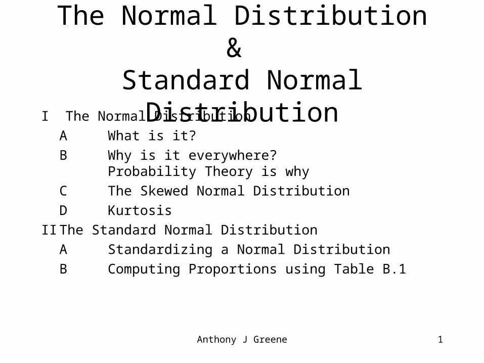
A Normal Distribution:Chest Sizes of Scottish Militia Men
0
200
400
600
800
1000
1200
33 34 35 36 37 38 39 40 41 42 43 44 45 46 47 48
Anthony J Greene 3
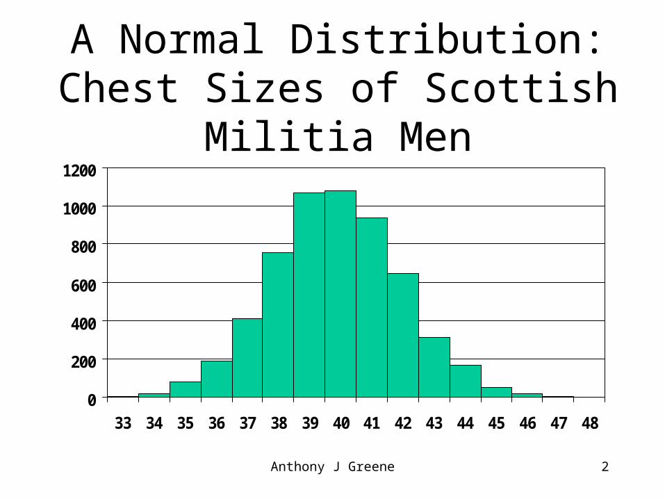
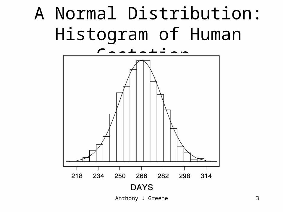
A Normal Distribution:Histogram of Human Gestation
Anthony J Greene 4
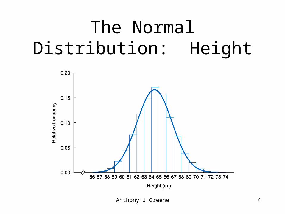
The Normal Distribution: Height
Anthony J Greene 5
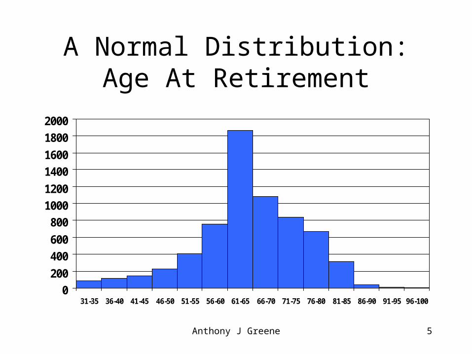
A Normal Distribution:Age At Retirement
0
200
400
600
800
1000
1200
1400
1600
1800
2000
31-35 36-40 41-45 46-50 51-55 56-60 61-65 66-70 71-75 76-80 81-85 86-90 91-95 96-100
Anthony J Greene 6
Normally Distributed Variables
• The most common continuous (interval/ratio) variable type
• Occurs predominantly in nature (biology, psychology, etc.)
• Determined by the principles of Probability

Anthony J Greene 7
Probability and the Normal Distribution
Probability is the Underlying Cause of the Normal Distribution
Anthony J Greene 8
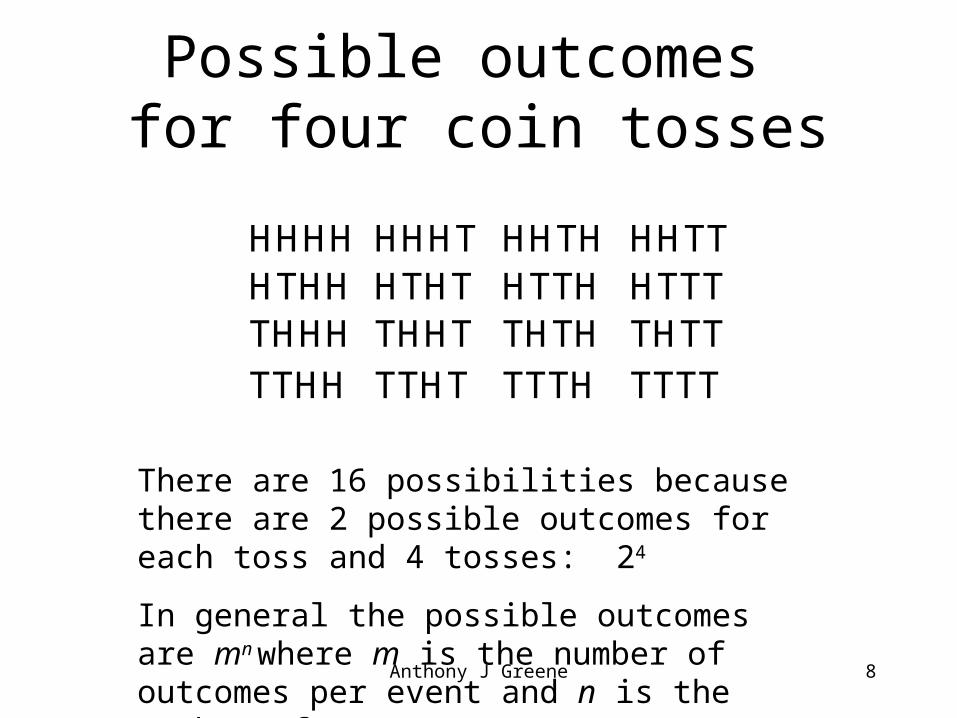
Possible outcomes for four coin tosses
HHHH HHHT HHTH HHTTHTHH HTHT HTTH HTTTTHHH THHT THTH THTTTTHH TTHT TTTH TTTT
There are 16 possibilities because there are 2 possible outcomes for each toss and 4 tosses: 24
In general the possible outcomes are mn where m is the number of outcomes per event and n is the number of events
Anthony J Greene 9
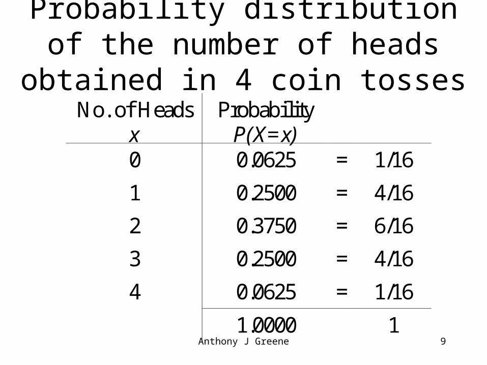
Probability distribution of the number of heads obtained in 4 coin tosses
No. of Headsx
ProbabilityP(X=x)
0 0.0625 = 1/16
1 0.2500 = 4/16
2 0.3750 = 6/16
3 0.2500 = 4/16
4 0.0625 = 1/16
1.0000 1
Anthony J Greene 10
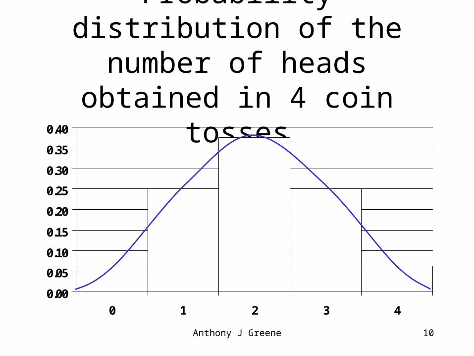
Probability distribution of the number of heads obtained in 4
coin tosses
0.00
0.05
0.10
0.15
0.20
0.25
0.30
0.35
0.40
0 1 2 3 4
Anthony J Greene 11
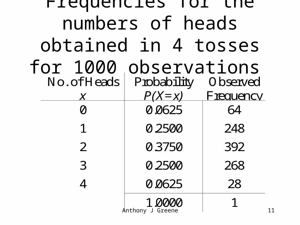
Frequencies for the numbers of heads obtained in 4 tosses for
1000 observations No. of Heads
xProbability
P(X=x)ObservedFrequency
0 0.0625 64
1 0.2500 248
2 0.3750 392
3 0.2500 268
4 0.0625 28
1.0000 1
Anthony J Greene 12
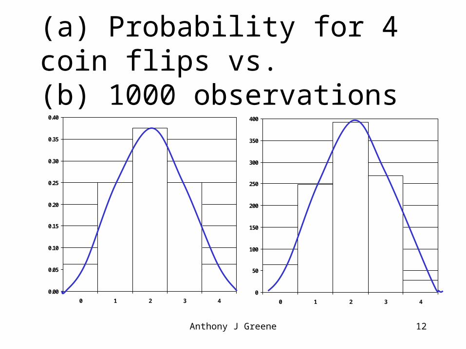
(a) Probability for 4 coin flips vs.
(b) 1000 observations
0.00
0.05
0.10
0.15
0.20
0.25
0.30
0.35
0.40
0 1 2 3 4
0
50
100
150
200
250
300
350
400
0 1 2 3 4
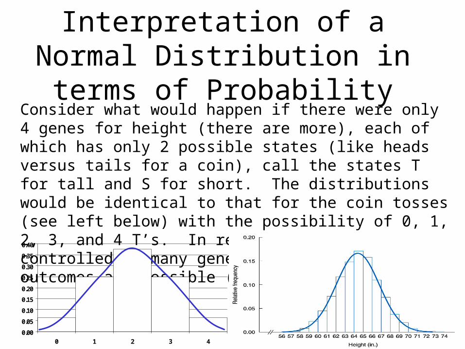
Interpretation of a Normal Distribution in terms of ProbabilityConsider what would happen if there were only 4 genes for height (there are more), each of which has only 2 possible states (like heads versus tails for a coin), call the states T for tall and S for short. The distributions would be identical to that for the coin tosses (see left below) with the possibility of 0, 1, 2, 3, and 4 T’s. In reality height is controlled by many genes so that more than 5 outcomes are possible (see right below).
0.00
0.05
0.10
0.15
0.20
0.25
0.30
0.35
0.40
0 1 2 3 4
Anthony J Greene 14
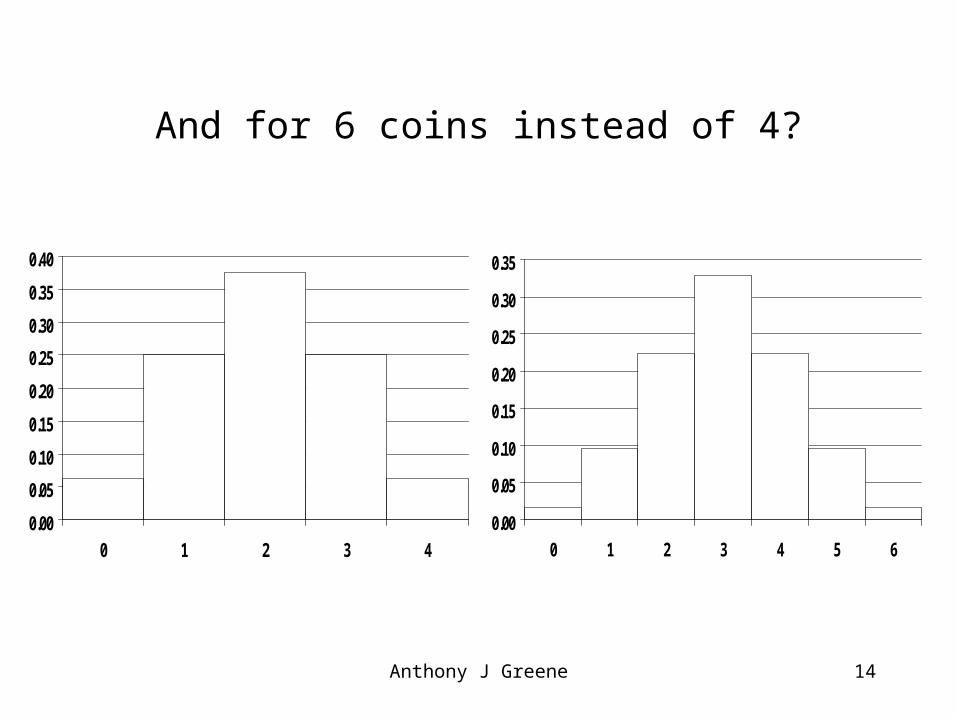
And for 6 coins instead of 4?
0.00
0.05
0.10
0.15
0.20
0.25
0.30
0.35
0.40
0 1 2 3 40.00
0.05
0.10
0.15
0.20
0.25
0.30
0.35
0 1 2 3 4 5 6
Anthony J Greene 15
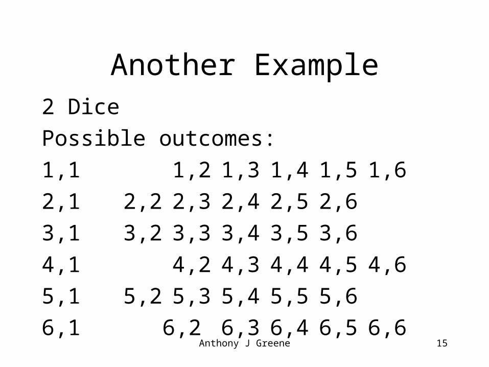
Another Example2 Dice
Possible outcomes:
1,1 1,2 1,3 1,4 1,5 1,6
2,1 2,2 2,3 2,4 2,5 2,6
3,1 3,2 3,3 3,4 3,5 3,6
4,1 4,2 4,3 4,4 4,5 4,6
5,1 5,2 5,3 5,4 5,5 5,6
6,1 6,2 6,3 6,4 6,5 6,6
Anthony J Greene 16
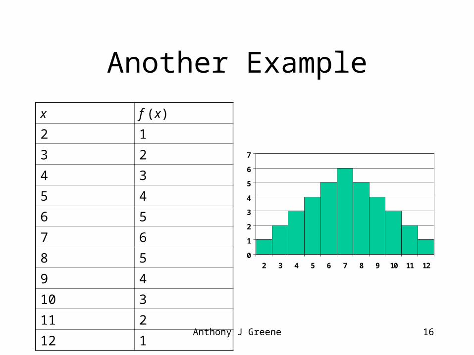
Another Example
x f (x)
2 1
3 2
4 3
5 4
6 5
7 6
8 5
9 4
10 3
11 2
12 1
0
1
2
3
4
5
6
7
2 3 4 5 6 7 8 9 10 11 12
Anthony J Greene 17
Examples of the Normal Distribution
• Age• Height• Weight• I.Q.• Sick Days per Year• Hours Sleep per Night• Words Read per
Minute
• Calories Eaten per Day• Hours of Work Done
per Day• Eyeblinks per Hour• Insulting Remarks per
Week• Number of Pairs of
Socks Owned
Anthony J Greene 18
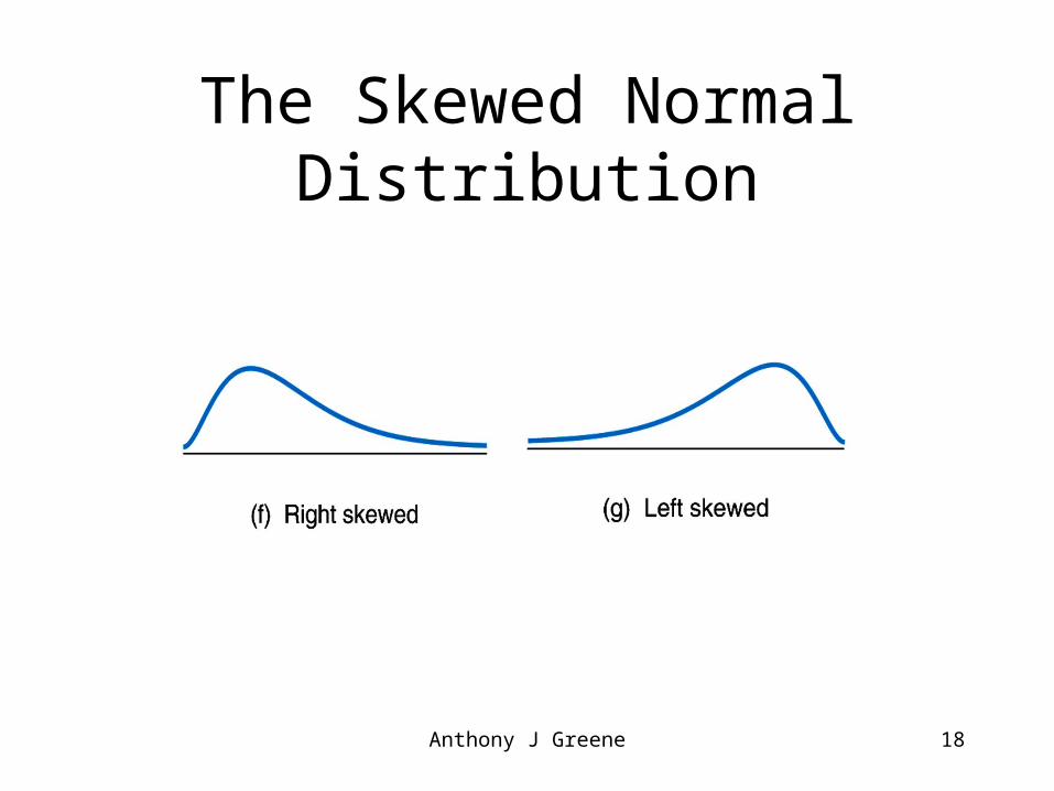
The Skewed Normal Distribution
Anthony J Greene 19
Examples of Skewed Normal Distributions
• Income• Number of Empty
Soda Cans in Car• Drug Use per Week• Car Accidents per
Year• Lifetime
Hospitalizations
• Number of Guitars Owned
• Consecutive Days Unemployed
• Hand-Washings per Day
• Number of Languages Spoken Fluently
• Hours of T.V. per Day
Anthony J Greene 20
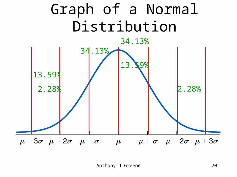
Graph of a Normal Distribution
34.13%
13.59%
2.28%
34.13%
13.59%
2.28%
Anthony J Greene 21
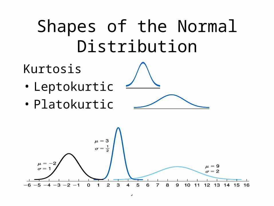
Shapes of the Normal Distribution
Kurtosis
• Leptokurtic
• Platokurtic
Anthony J Greene 22
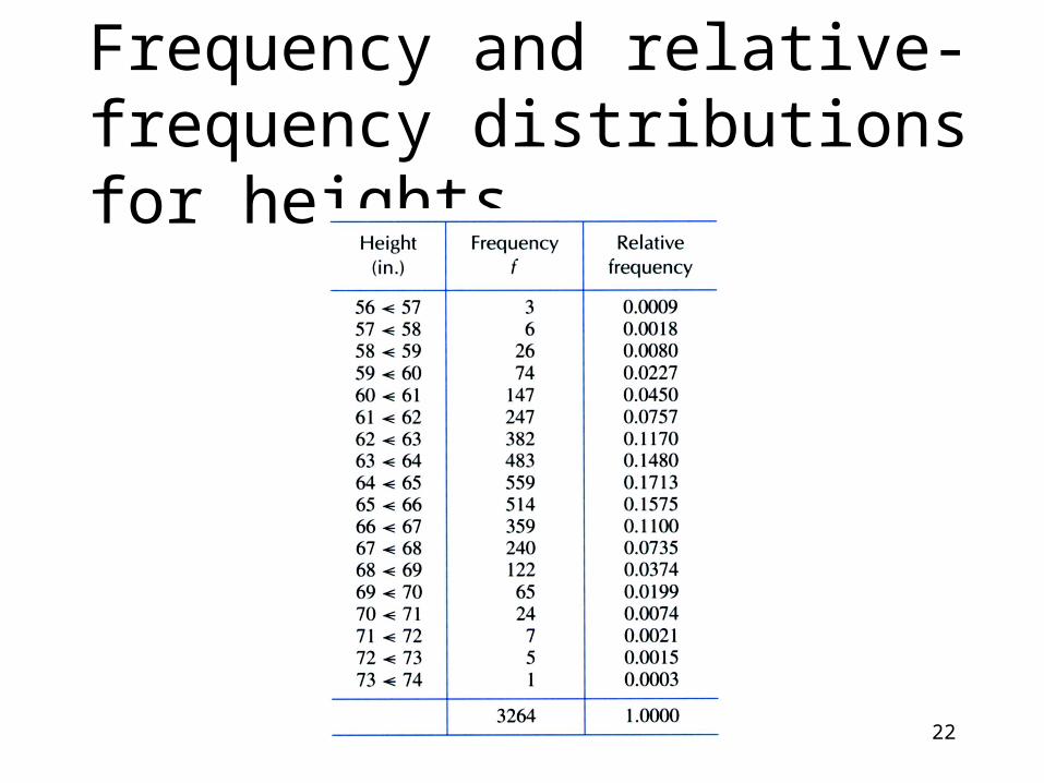
Frequency and relative-frequency distributions for heights
Anthony J Greene 23
What do we do with Normal Distributions?
1. Determine the position of a given score relative to all other scores.
2. Compare distributions.
Anthony J Greene 24
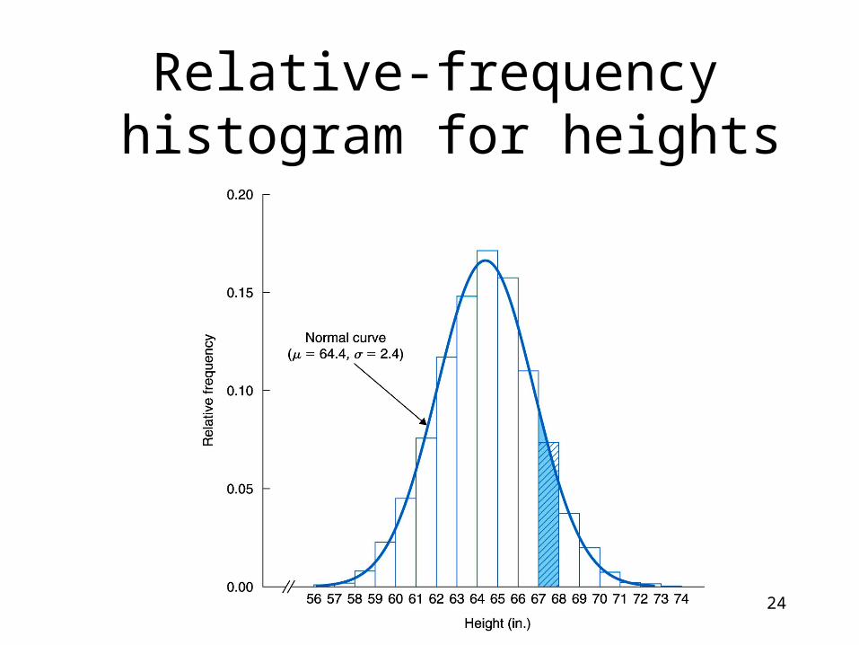
Relative-frequency histogram for heights
Anthony J Greene 25
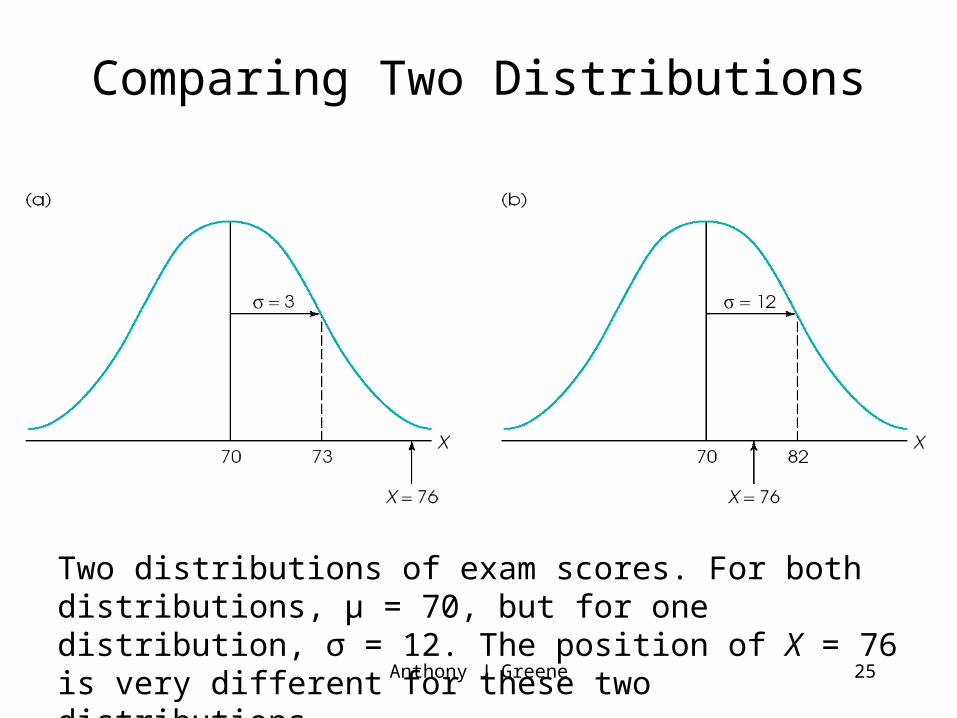
Comparing Two Distributions
Two distributions of exam scores. For both distributions, µ = 70, but for one distribution, σ = 12. The position of X = 76 is very different for these two distributions.
Anthony J Greene 26
Data Transformations are Reversible and Do not Alter the
Relations Among Items1) Add or Subtract a Constant From Each
Score2) Multiply Each Score By a Constant
• e.g., if you wanted to convert a group of Fahrenheit temperatures to Centigrade you would subtract 32 from each score then multiply by 5/9ths
Anthony J Greene 27
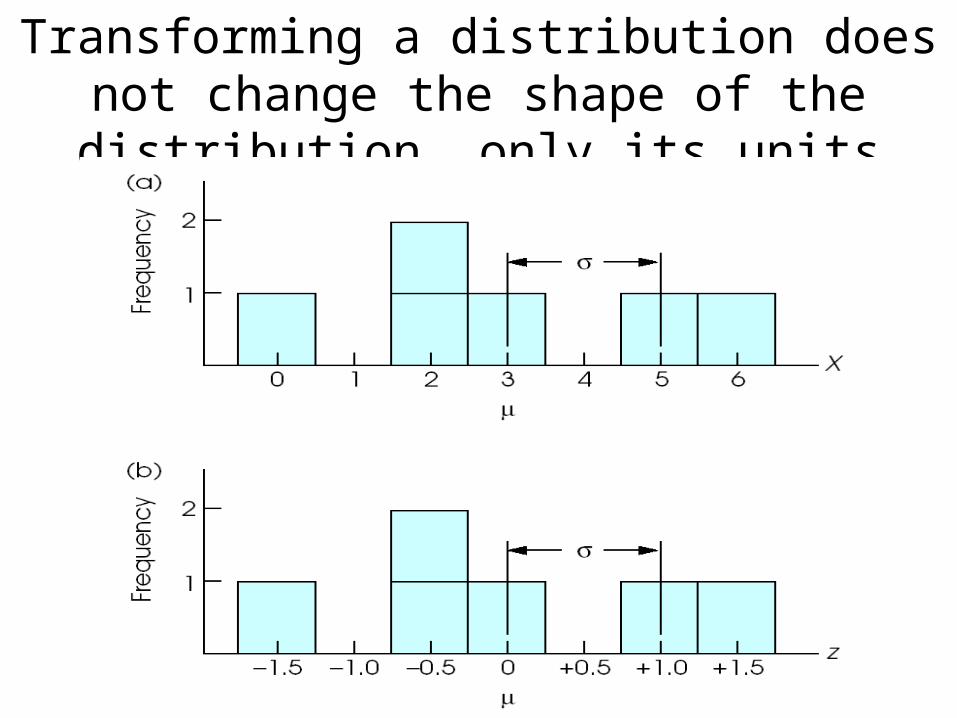
Transforming a distribution does not change the shape of the distribution, only its units
Anthony J Greene 28
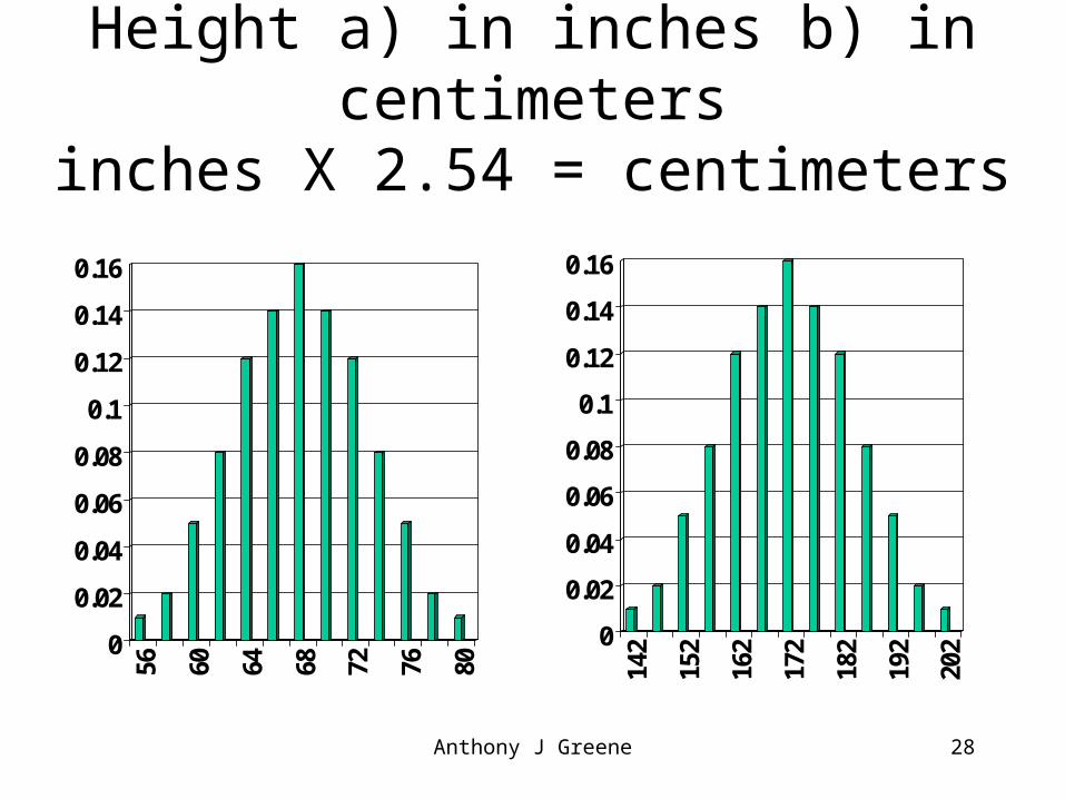
Height a) in inches b) in centimetersinches X 2.54 = centimeters
0
0.02
0.04
0.06
0.08
0.1
0.12
0.14
0.16
56 60 64 68 72 76 80
0
0.02
0.04
0.06
0.08
0.1
0.12
0.14
0.16
142
152
162
172
182
192
202
Anthony J Greene 29
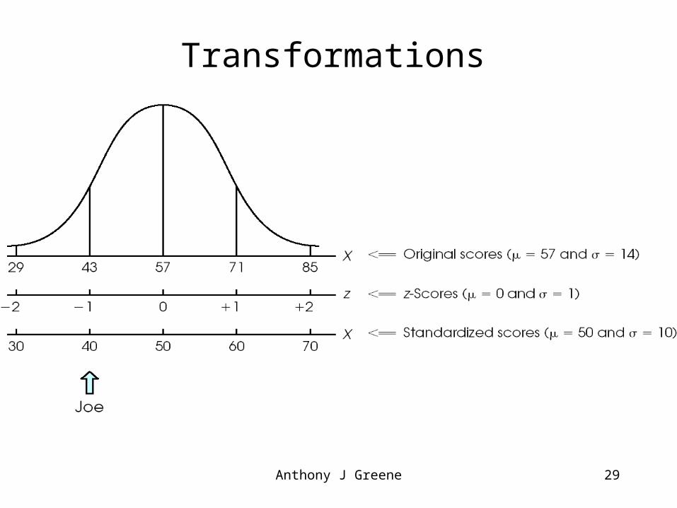
Transformations
Anthony J Greene 30
Standard Normal Distribution
A normally distributed variable having mean 0 and standard deviation 1 is said to have the standard normal distribution. Its associated normal curve is called the standard normal curve.
Anthony J Greene 31
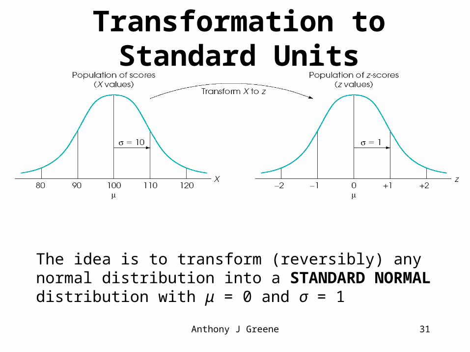
Transformation to Standard Units
The idea is to transform (reversibly) any normal distribution into a STANDARD NORMAL distribution with μ = 0 and σ = 1
Anthony J Greene 32
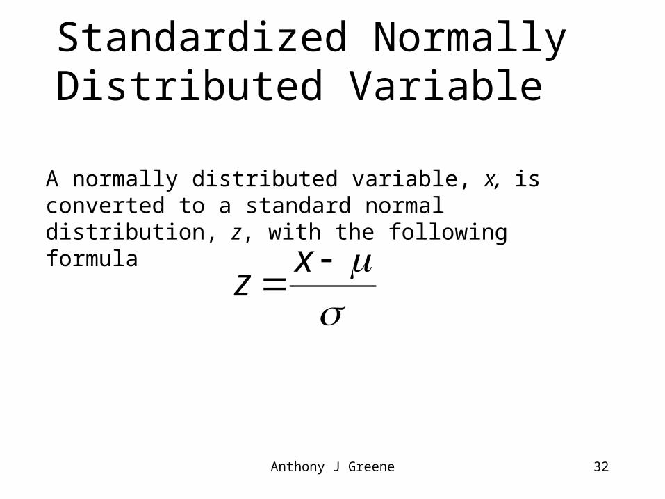
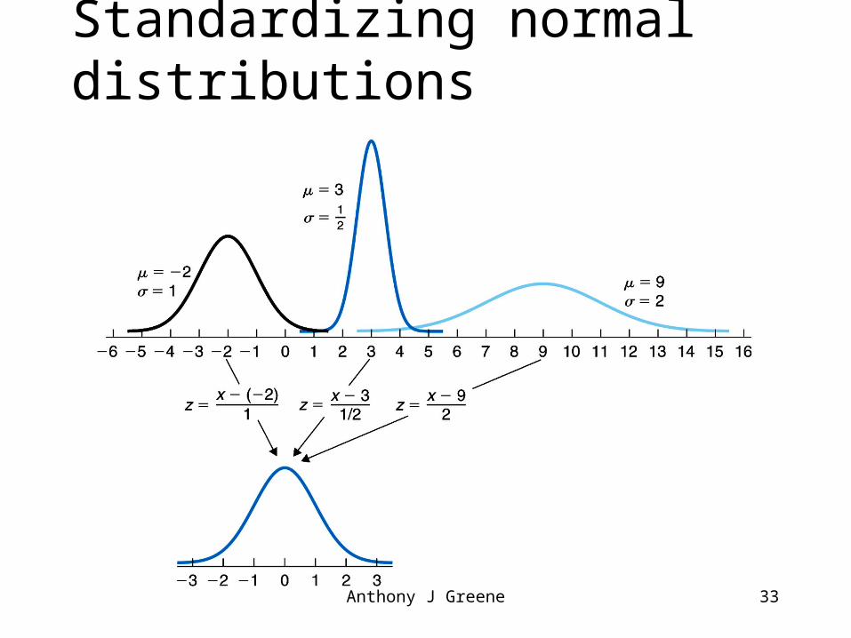
Standardized Normally Distributed Variable
A normally distributed variable, x, is converted to a standard normal distribution, z, with the following formula
x
z
Anthony J Greene 33
Standardizing normal distributions
Anthony J Greene 34
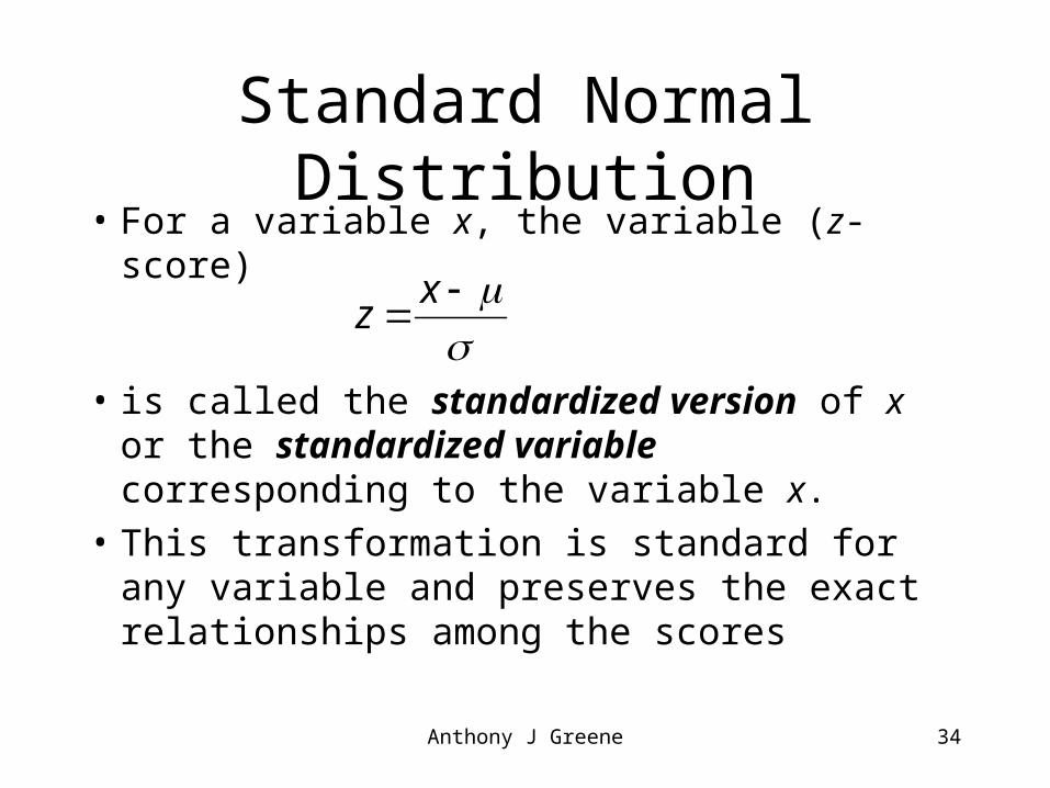
Standard Normal Distribution• For a variable x, the variable (z-score)
• is called the standardized version of x or the standardized variable corresponding to the variable x.
• This transformation is standard for any variable and preserves the exact relationships among the scores
x
z
Anthony J Greene 35
Standard Normal Distributions
• The z-score transformation is entirely reversible but allows any distribution to be compared (e.g., I.Q. and SAT score; does a top I.Q. score correspond to a top SAT score?)
• z-scores all have a mean of zero and a standard deviation of 1, which gives them the simplest possible mathematical properties.
Anthony J Greene 36
Standard Normal Distributions
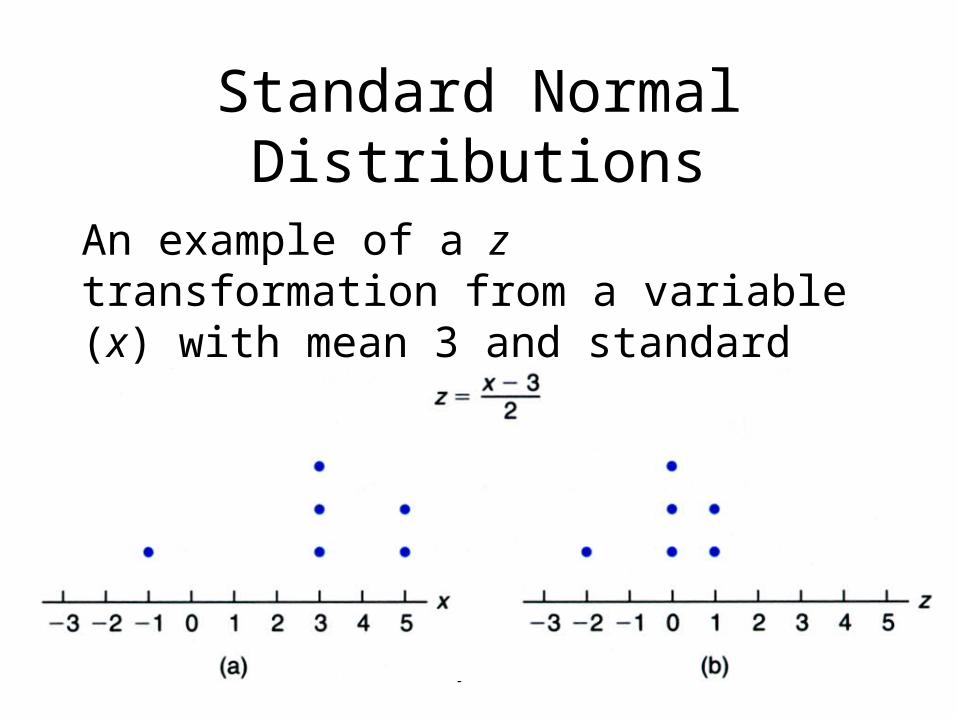
An example of a z transformation from a variable (x) with mean 3 and standard deviation 2
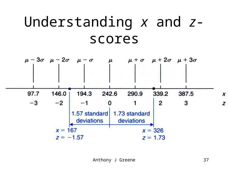
Anthony J Greene 37
Understanding x and z-scores
Anthony J Greene 38
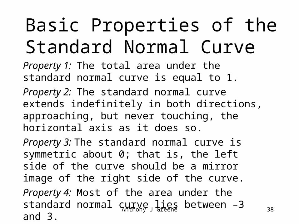
Basic Properties of the Standard Normal Curve Property 1: The total area under the standard normal curve is equal to 1.
Property 2: The standard normal curve extends indefinitely in both directions, approaching, but never touching, the horizontal axis as it does so.
Property 3: The standard normal curve is symmetric about 0; that is, the left side of the curve should be a mirror image of the right side of the curve.
Property 4: Most of the area under the standard normal curve lies between –3 and 3.
Anthony J Greene 39
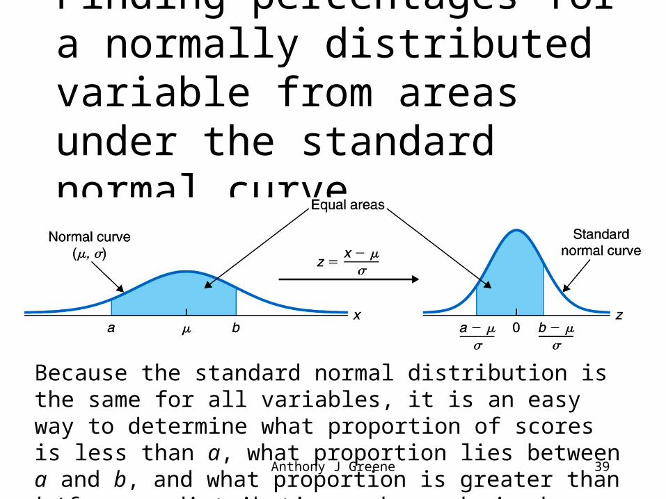
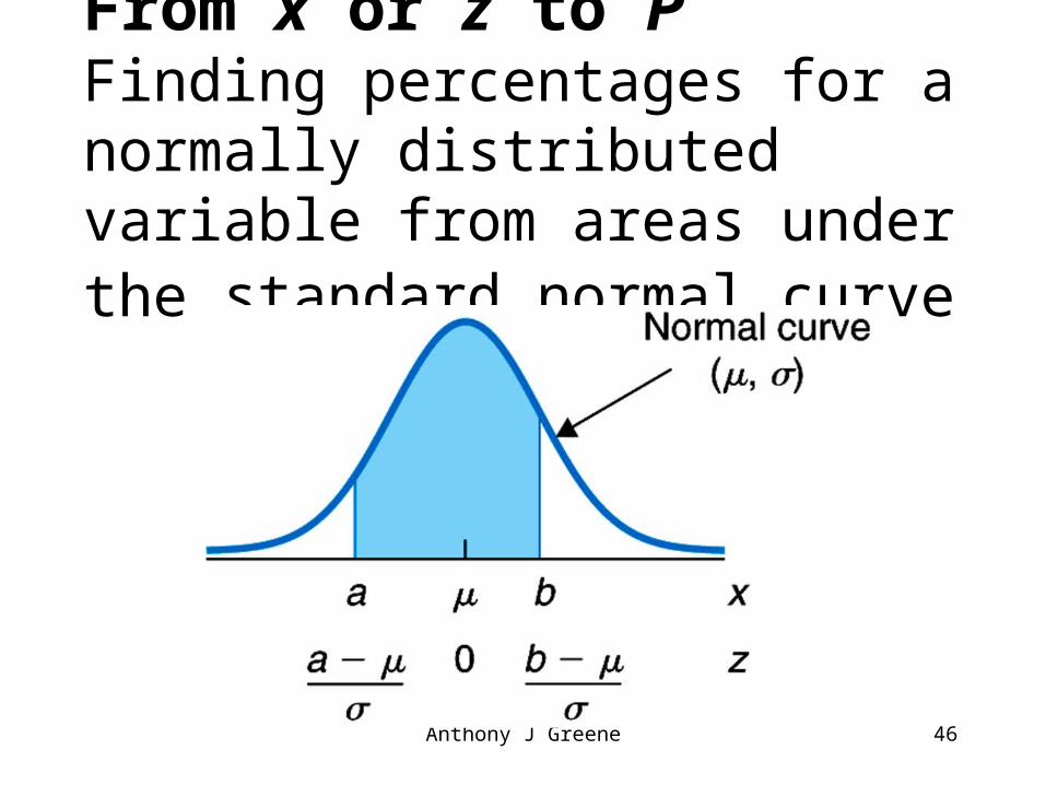
Finding percentages for a normally distributed variable from areas under the standard normal curve
Because the standard normal distribution is the same for all variables, it is an easy way to determine what proportion of scores is less than a, what proportion lies between a and b, and what proportion is greater than b (for any distribution and any desired points a and b).
Anthony J Greene 40
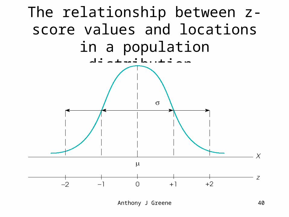
The relationship between z-score values and locations in a population
distribution.
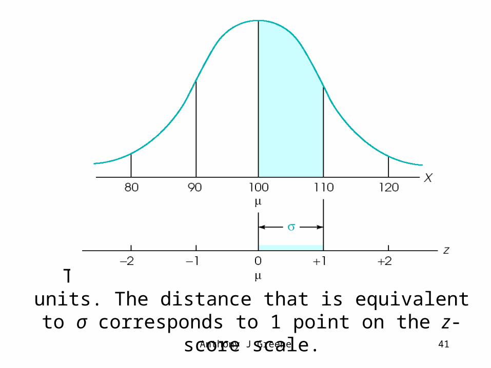
Anthony J Greene 41
The X-axis is relabeled in z-score units. The distance that is equivalent to σ corresponds to 1 point on the z-score scale.
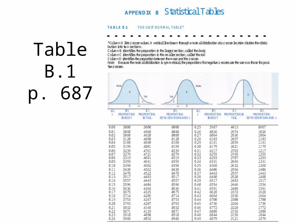
Table B.1
p. 687
Anthony J Greene 43
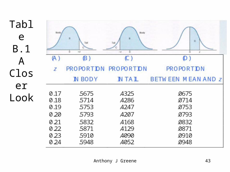
Table B.1A
Closer Look
Anthony J Greene 44
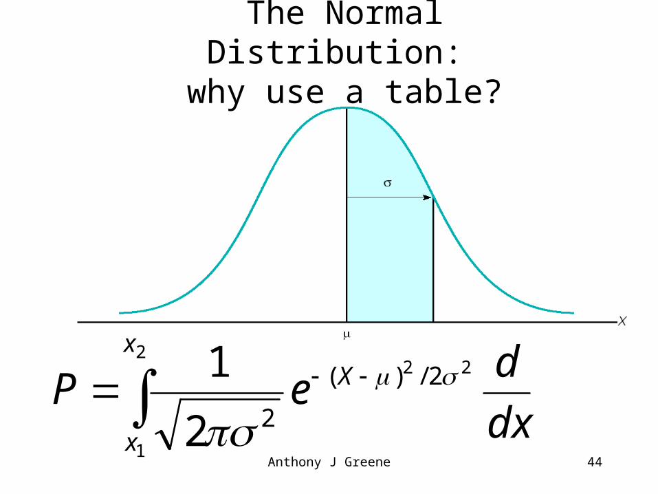
dx
deP
x
x
X 2
1
22 2/)(
22
1
The Normal Distribution: why use a table?
Anthony J Greene 45
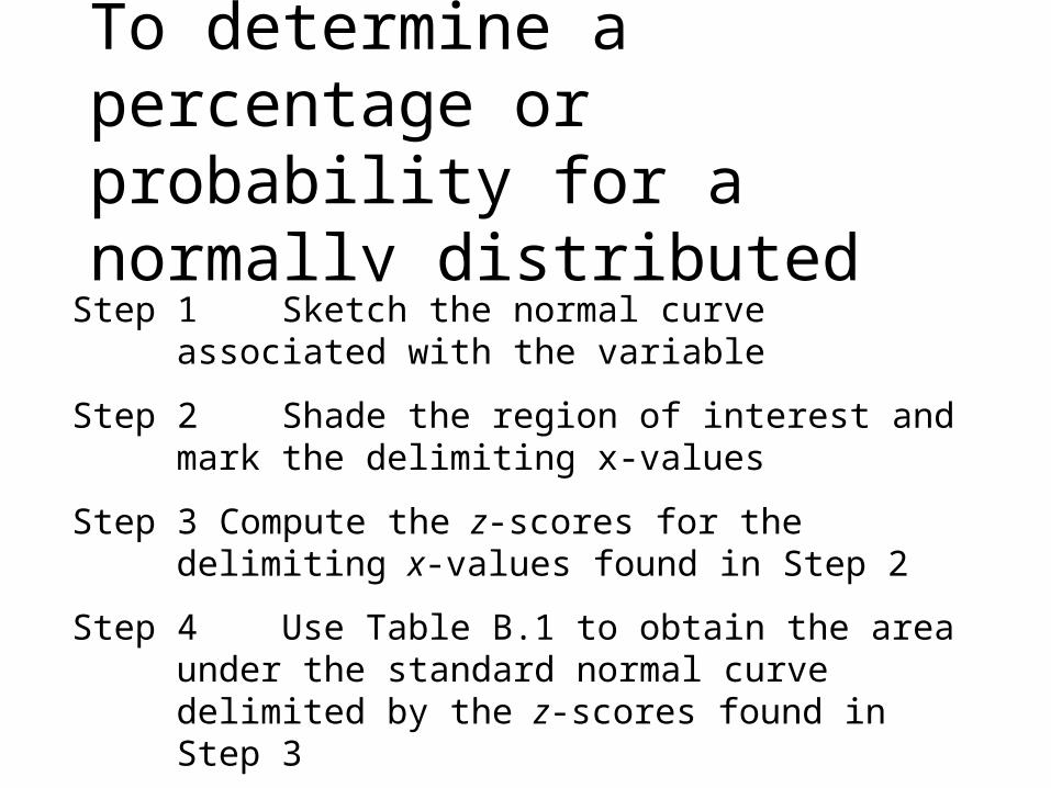
From x or z to PTo determine a percentage orprobability for a normally distributed variable
Step 1 Sketch the normal curve associated with the variable
Step 2 Shade the region of interest and mark the delimiting x-values
Step 3 Compute the z-scores for the delimiting x-values found in Step 2
Step 4 Use Table B.1 to obtain the area under the standard normal curve delimited by the z-scores found in Step 3
Use Geometry and remember that the total area under the curve is always 1.00.
Anthony J Greene 46
From x or z to PFinding percentages for a normally distributed variable from areas under the standard normal curve
Anthony J Greene 47
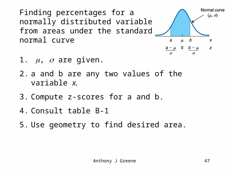
Finding percentages for a normally distributed variable from areas under the standard normal curve
1. , are given.
2. a and b are any two values of the variable x.
3. Compute z-scores for a and b.
4. Consult table B-1
5. Use geometry to find desired area.
Anthony J Greene 48
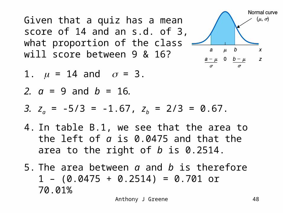
Given that a quiz has a mean score of 14 and an s.d. of 3, what proportion of the class will score between 9 & 16?
1. = 14 and = 3.
2. a = 9 and b = 16.
3. za = -5/3 = -1.67, zb = 2/3 = 0.67.
4. In table B.1, we see that the area to the left of a is 0.0475 and that the area to the right of b is 0.2514.
5. The area between a and b is therefore 1 – (0.0475 + 0.2514) = 0.701 or 70.01%
Anthony J Greene 49
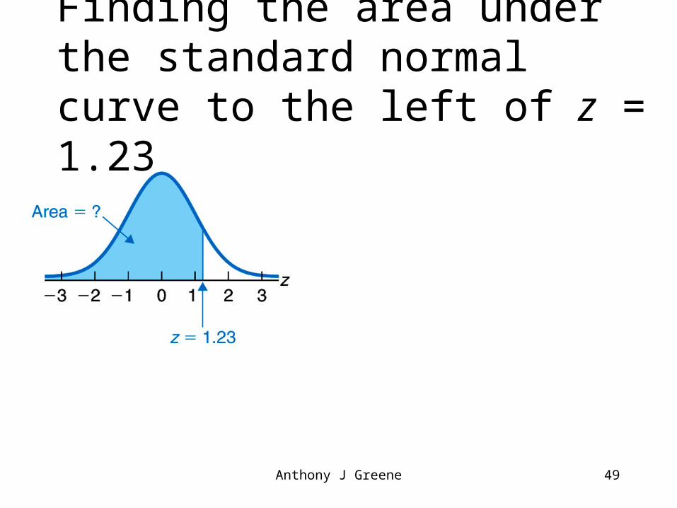
Finding the area under the standard normal curve to the left of z = 1.23
Anthony J Greene 50
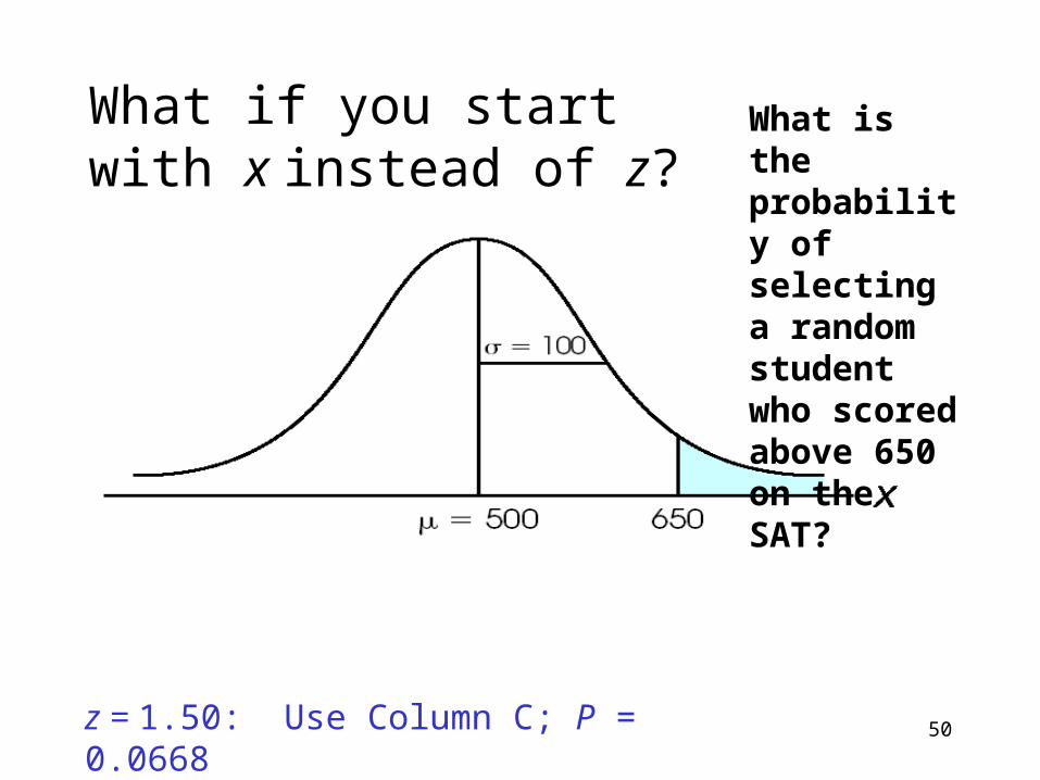
What if you start with x instead of z?
z = 1.50: Use Column C; P = 0.0668
What is the probability of selecting a random student who scored above 650 on the SAT?
Anthony J Greene 51
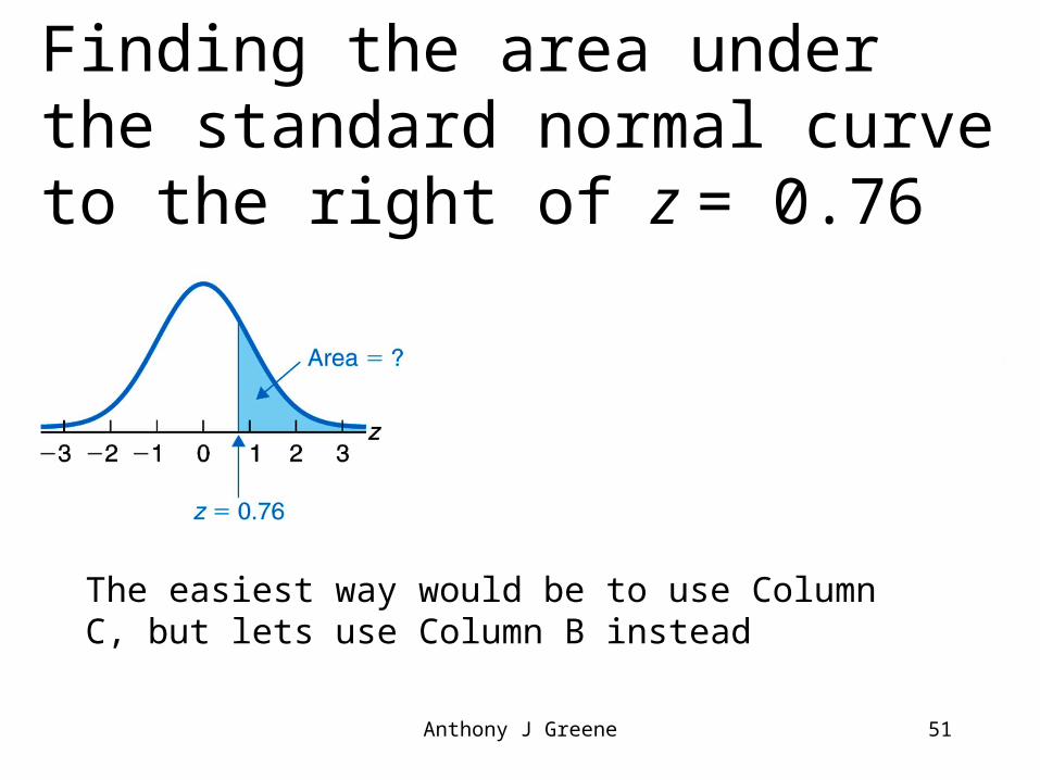
Finding the area under the standard normal curve to the right of z = 0.76
The easiest way would be to use Column C, but lets use Column B instead
Anthony J Greene 52
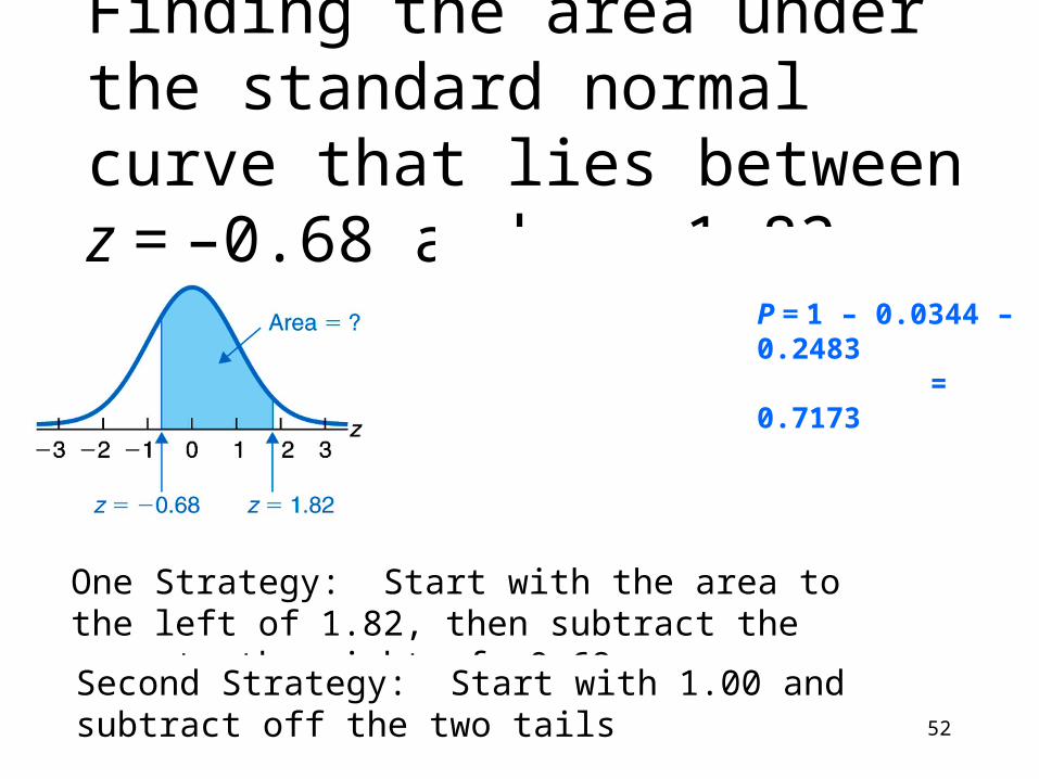
Finding the area under the standard normal curve that lies between z = –0.68 and z = 1.82
One Strategy: Start with the area to the left of 1.82, then subtract the area to the right of -0.68.
P = 1 – 0.0344 – 0.2483 = 0.7173
Second Strategy: Start with 1.00 and subtract off the two tails
Anthony J Greene 53
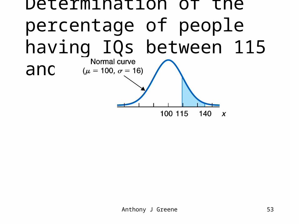
Determination of the percentage of people having IQs between 115 and 140
Anthony J Greene 54
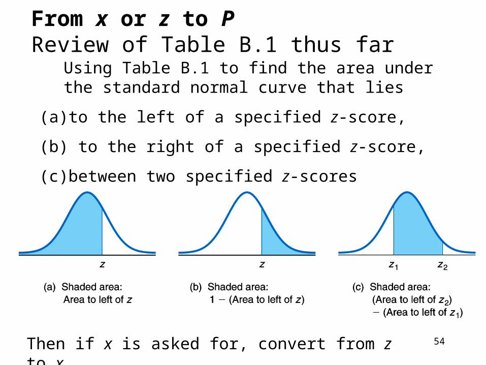
From x or z to PReview of Table B.1 thus far
Using Table B.1 to find the area under the standard normal curve that lies
(a) to the left of a specified z-score,
(b) to the right of a specified z-score,
(c) between two specified z-scores
Then if x is asked for, convert from z to x
Anthony J Greene 55
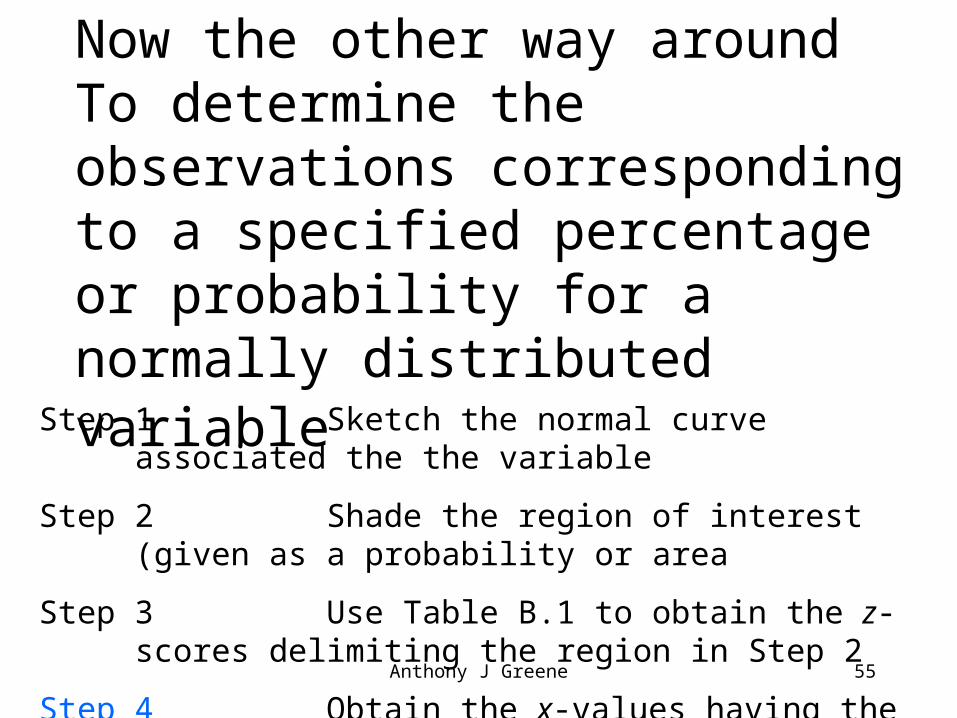
From P to z or x Now the other way around
To determine the observations corresponding to a specified percentage or probability for a normally distributed variable
Step 1 Sketch the normal curve associated the the variable
Step 2 Shade the region of interest (given as a probability or area
Step 3 Use Table B.1 to obtain the z-scores delimiting the region in Step 2
Step 4 Obtain the x-values having the z-scores found in Step 3
Anthony J Greene 56
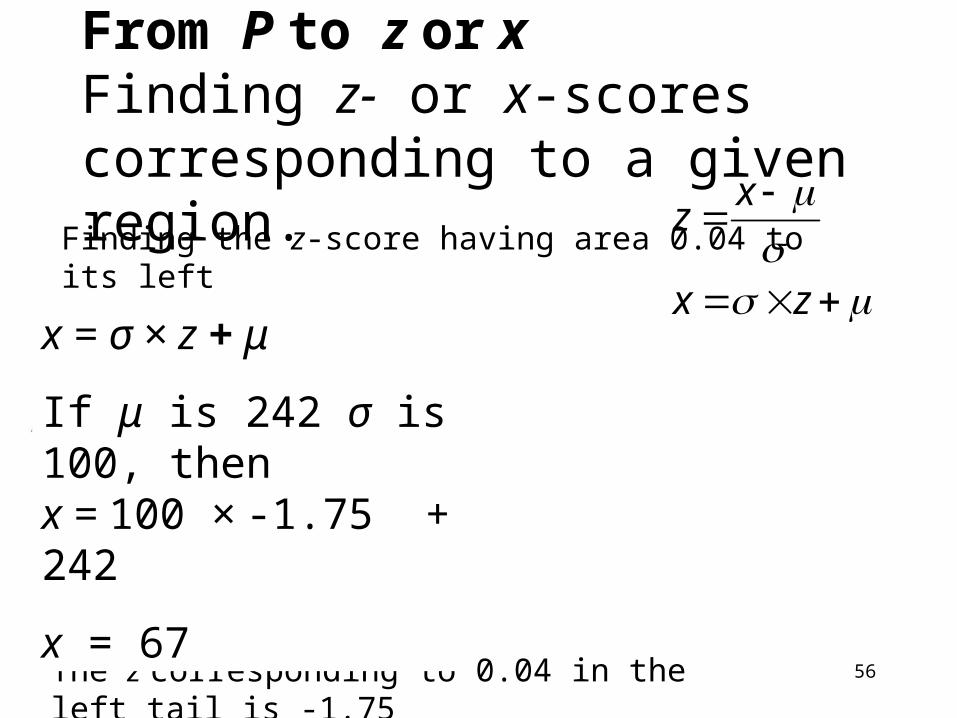
From P to z or xFinding z- or x-scores corresponding to a given region.
Finding the z-score having area 0.04 to its left
Use Column C: The z corresponding to 0.04 in the left tail is -1.75
x = σ × z + μ
If μ is 242 σ is 100, thenx = 100 × -1.75 + 242
x = 67
zx
xz
Anthony J Greene 57
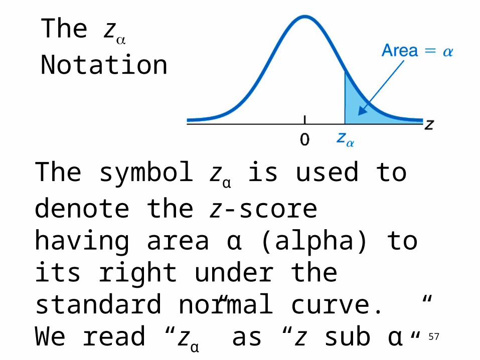
The z Notation
The symbol zα is used to denote the z-score having area α (alpha) to its right under the standard normal curve. We read “zα” as “z sub α” or more simply as “z α.”

Anthony J Greene 58
The z notation : P(X>x) = α
This is the z-score that demarks an area under the curve with P(X>x)= α
P(X>x)= α
Anthony J Greene 59
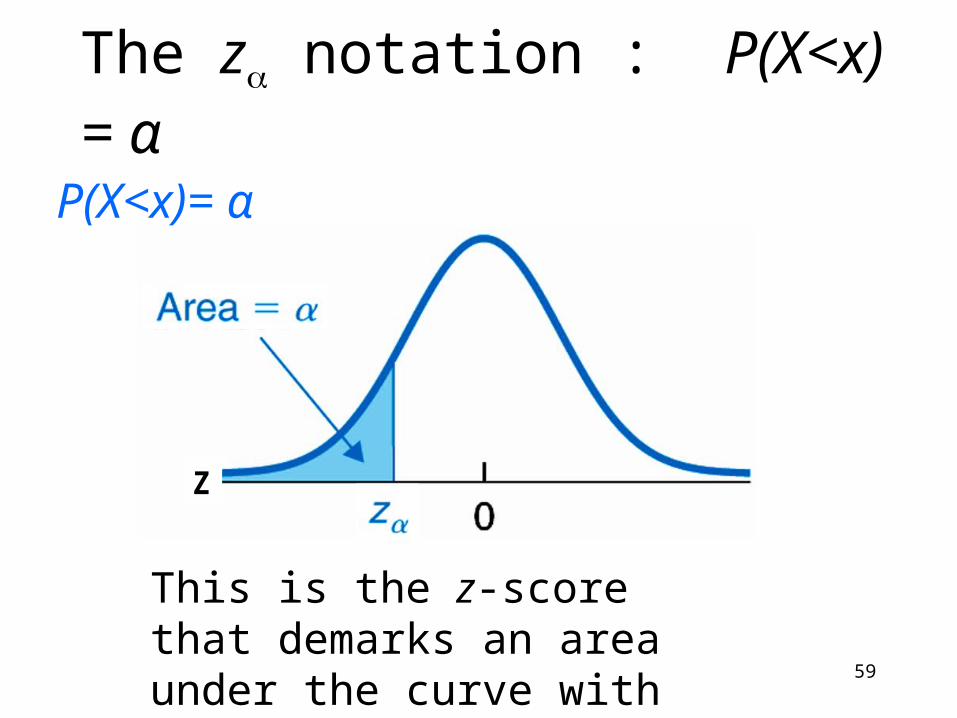
The z notation : P(X<x) = α
This is the z-score that demarks an area under the curve with P(X<x)= α
P(X<x)= α
Z
Anthony J Greene 60
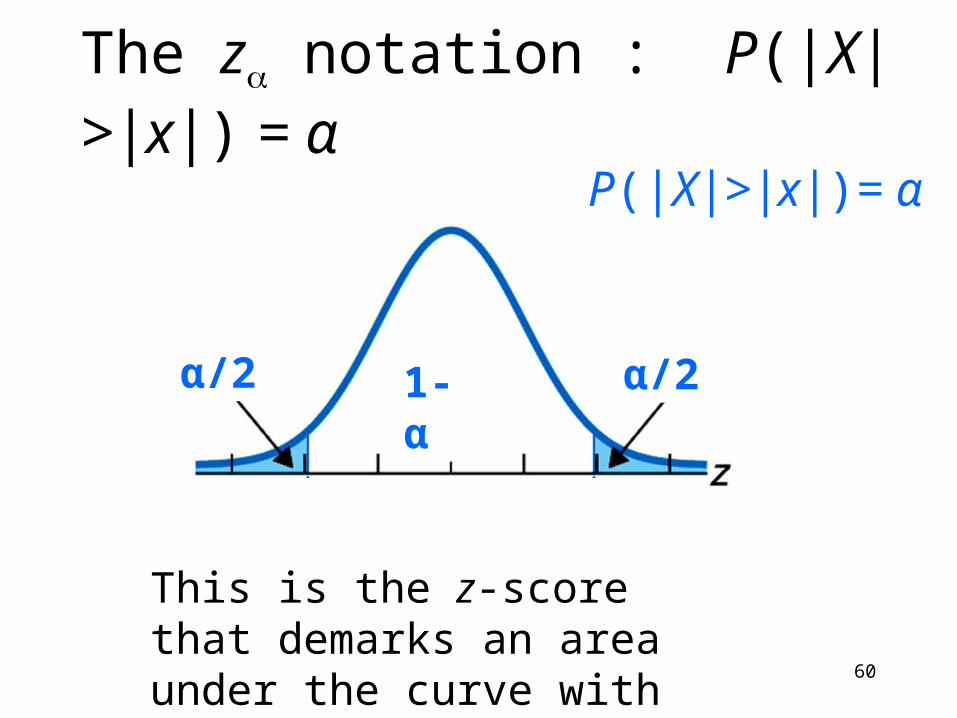
The z notation : P(|X|>|x|) = α
This is the z-score that demarks an area under the curve with P(|X|>|x|)= α
P(|X|>|x|)= α
α/2 α/21- α
Anthony J Greene 61
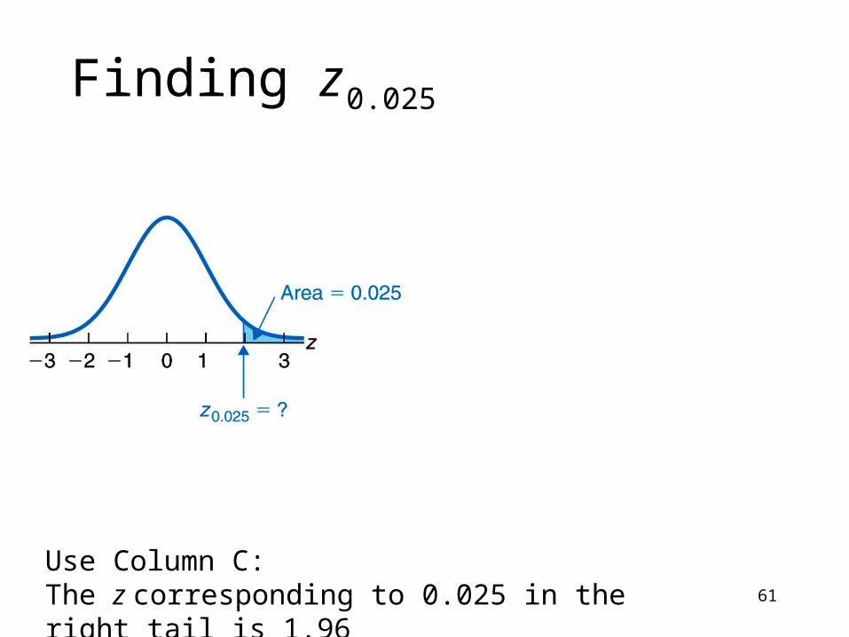
Finding z 0.025
Use Column C: The z corresponding to 0.025 in the right tail is 1.96
Anthony J Greene 62
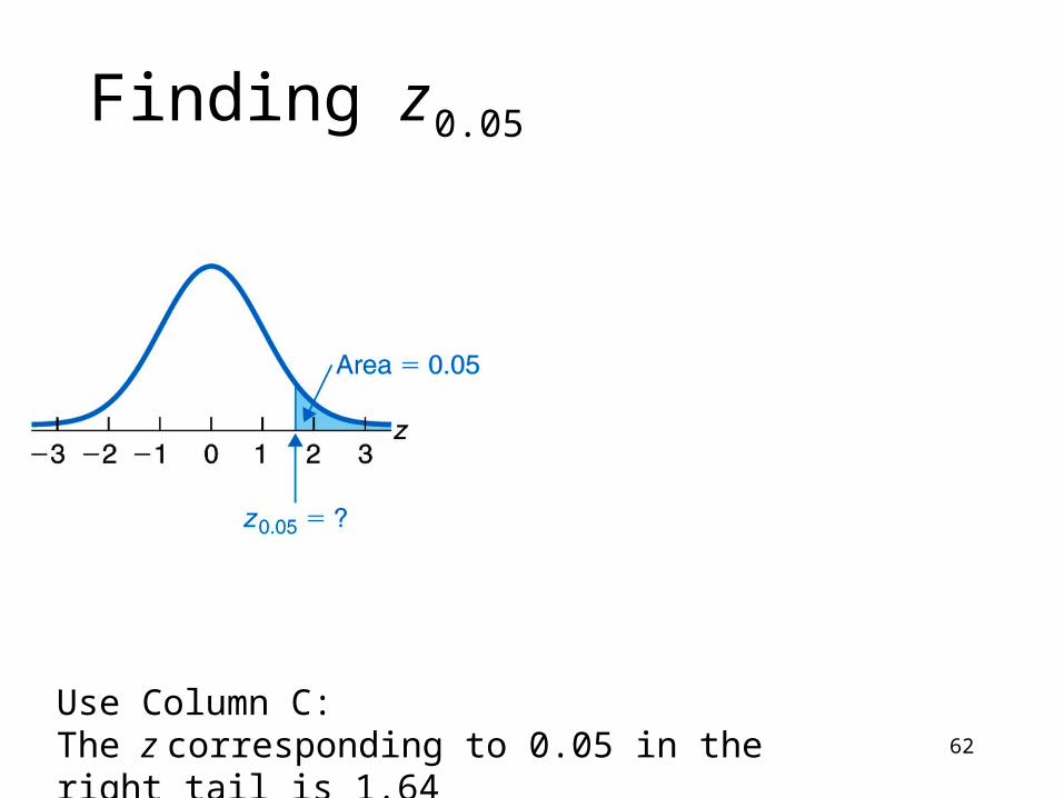
Finding z 0.05
Use Column C: The z corresponding to 0.05 in the right tail is 1.64
Anthony J Greene 63
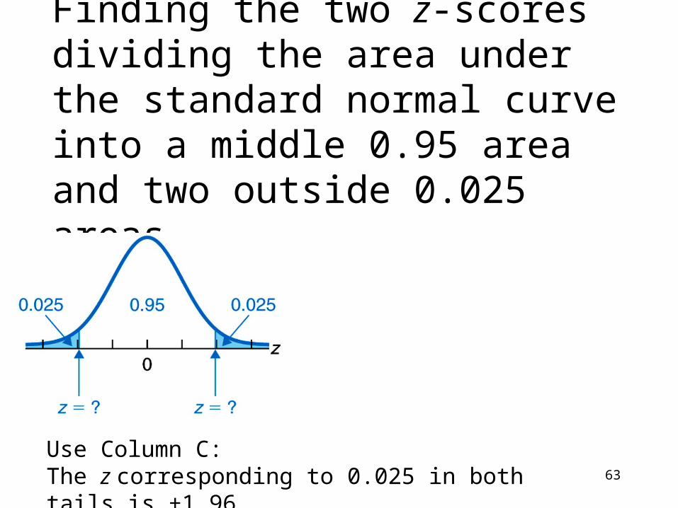
Finding the two z-scores dividing the area under the standard normal curve into a middle 0.95 area and two outside 0.025 areas
Use Column C: The z corresponding to 0.025 in both tails is ±1.96
Anthony J Greene 64
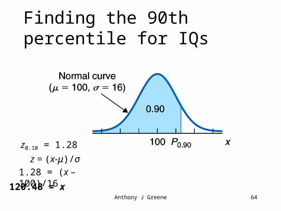
Finding the 90th percentile for IQs
z0.10 = 1.28
z = (x-μ)/σ
1.28 = (x – 100)/16
120.48 = x
Anthony J Greene 65
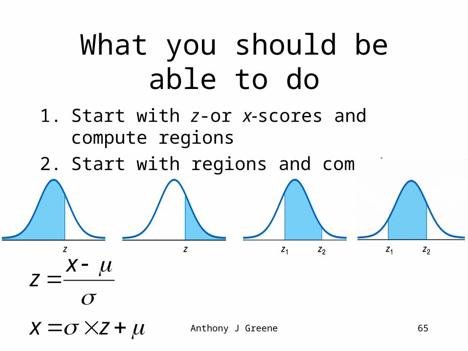
What you should be able to do
1. Start with z-or x-scores and compute regions
2. Start with regions and compute z- or x-scores
zx
xz
Anthony J Greene 66
DESCRIPTIVES EXERCISE & REVIEW
Anthony J Greene
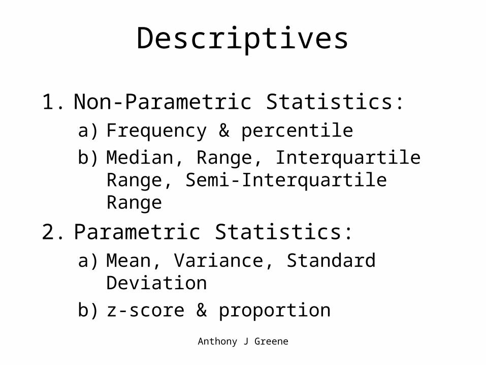
Descriptives
1. Non-Parametric Statistics: a) Frequency & percentile
b) Median, Range, Interquartile Range, Semi-Interquartile Range
2. Parametric Statistics: a) Mean, Variance, Standard Deviation
b) z-score & proportion
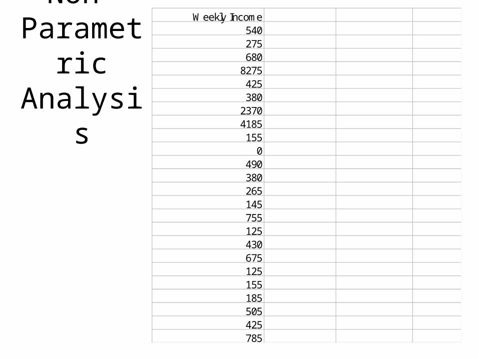
Non-Parametric Analysis
Weekly Income540275680
8275425380
23704185155
0490380265145755125430675125155185505425785
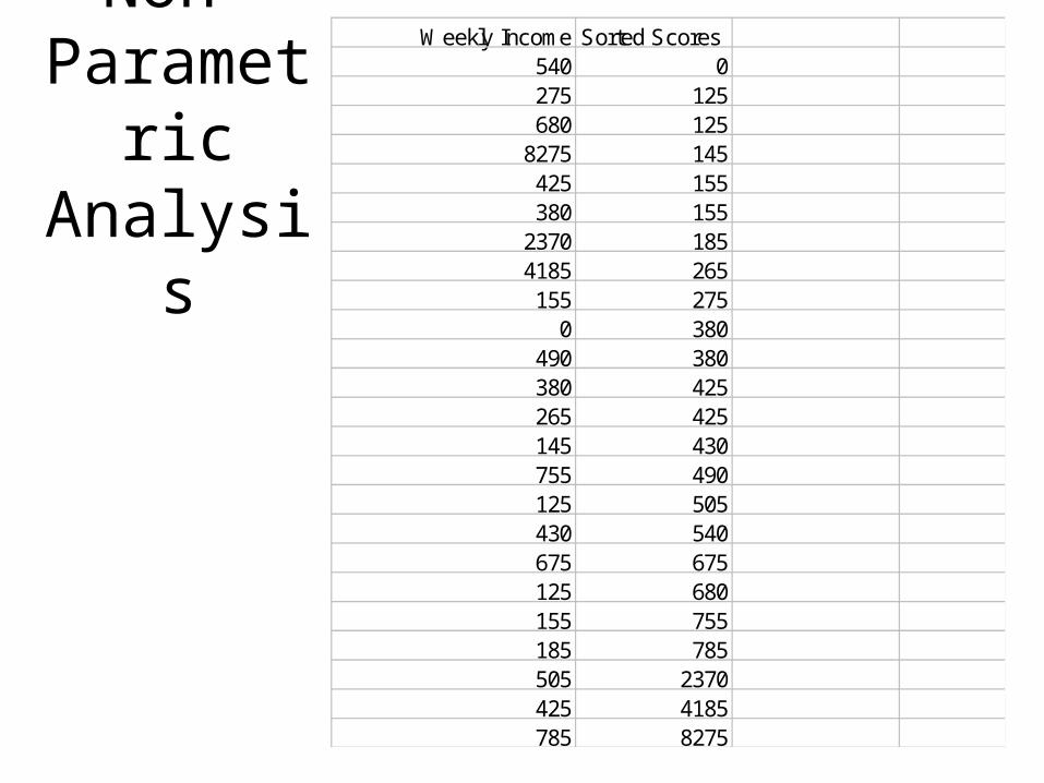
Non-Parametric Analysis
Weekly Income Sorted Scores540 0275 125680 125
8275 145425 155380 155
2370 1854185 265155 275
0 380490 380380 425265 425145 430755 490125 505430 540675 675125 680155 755185 785505 2370425 4185785 8275
Non-Parametric Analysis
Weekly Income Sorted Scores540 0275 125680 125
8275 145425 155380 155
2370 1854185 265155 275
0 380490 380380 425265 425145 430755 490125 505430 540675 675125 680155 755185 785505 2370425 4185785 8275
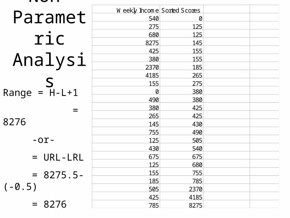
Range = H-L+1
= 8276
-or-
= URL-LRL
= 8275.5-(-0.5)
= 8276
Non-Parametric Analysis
Weekly Income Sorted Scores 25%, 50%, 75%540 0275 125680 125
8275 145425 155380 155 155
2370 185 1854185 265155 275
0 380490 380380 425 425265 425 425145 430755 490125 505430 540675 675 675125 680 680155 755185 785505 2370425 4185785 8275
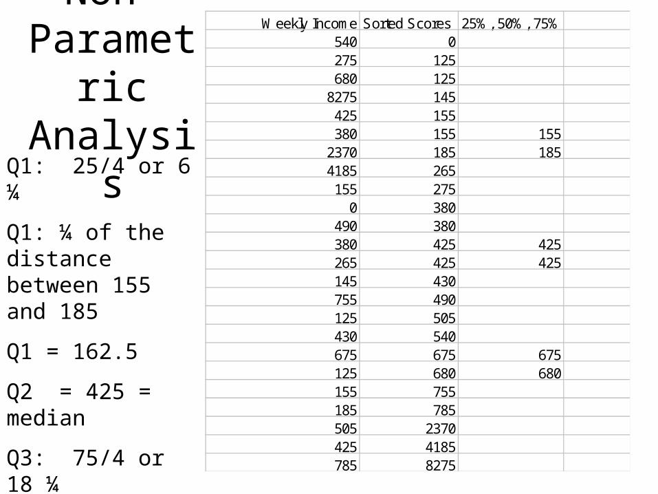
Q1: 25/4 or 6 ¼
Q1: ¼ of the distance between 155 and 185
Q1 = 162.5
Q2 = 425 = median
Q3: 75/4 or 18 ¼
Q3: ¼ of the distance between 675 and 680
Q3 = 676.25
Non-Parametric Analysis
Weekly Income Sorted Scores 25%, 50%, 75%540 0275 125680 125
8275 145425 155380 155 155
2370 185 1854185 265155 275
0 380490 380380 425 425265 425 425145 430755 490125 505430 540675 675 675125 680 680155 755185 785505 2370425 4185785 8275
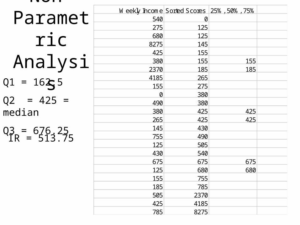
Q1 = 162.5
Q2 = 425 = median
Q3 = 676.25
IR = 513.75
Non-Parametric Analysis
Weekly Income Sorted Scores 25%, 50%, 75%540 0275 125680 125
8275 145425 155380 155 155
2370 185 1854185 265155 275
0 380490 380380 425 425265 425 425145 430755 490125 505430 540675 675 675125 680 680155 755185 785505 2370425 4185785 8275
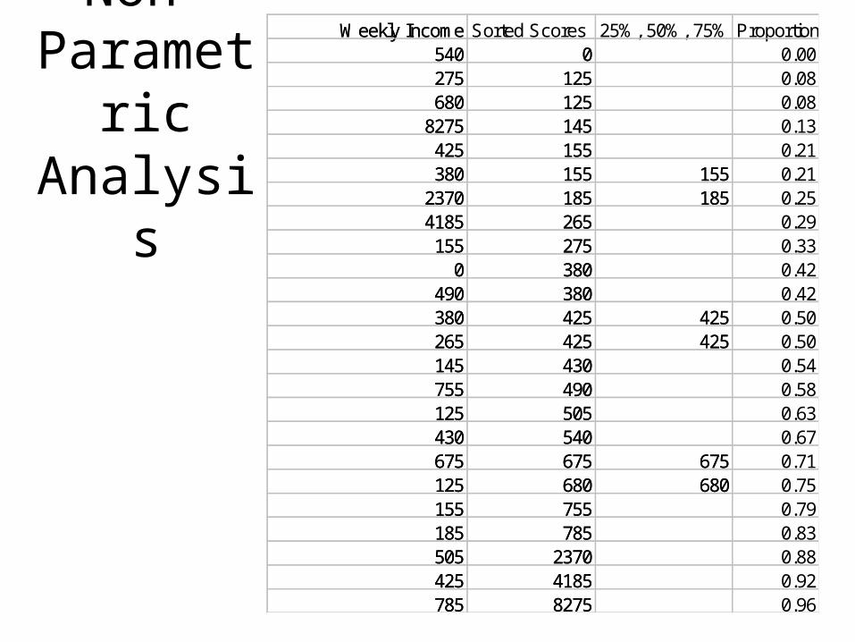
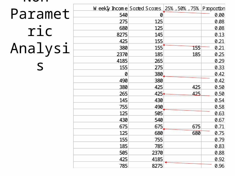
Weekly Income Proportion540 0 0.00275 125 0.08680 125 0.08
8275 145 0.13425 155 0.21380 155 155 0.21
2370 185 185 0.254185 265 0.29155 275 0.33
0 380 0.42490 380 0.42380 425 425 0.50265 425 425 0.50145 430 0.54755 490 0.58125 505 0.63430 540 0.67675 675 675 0.71125 680 680 0.75155 755 0.79185 785 0.83505 2370 0.88425 4185 0.92785 8275 0.96
Non-Parametric Analysis
Weekly Income Sorted Scores 25%, 50%, 75%540 0275 125680 125
8275 145425 155380 155 155
2370 185 1854185 265155 275
0 380490 380380 425 425265 425 425145 430755 490125 505430 540675 675 675125 680 680155 755185 785505 2370425 4185785 8275
Weekly Income Proportion540 0 0.00275 125 0.08680 125 0.08
8275 145 0.13425 155 0.21380 155 155 0.21
2370 185 185 0.254185 265 0.29155 275 0.33
0 380 0.42490 380 0.42380 425 425 0.50265 425 425 0.50145 430 0.54755 490 0.58125 505 0.63430 540 0.67675 675 675 0.71125 680 680 0.75155 755 0.79185 785 0.83505 2370 0.88425 4185 0.92785 8275 0.96
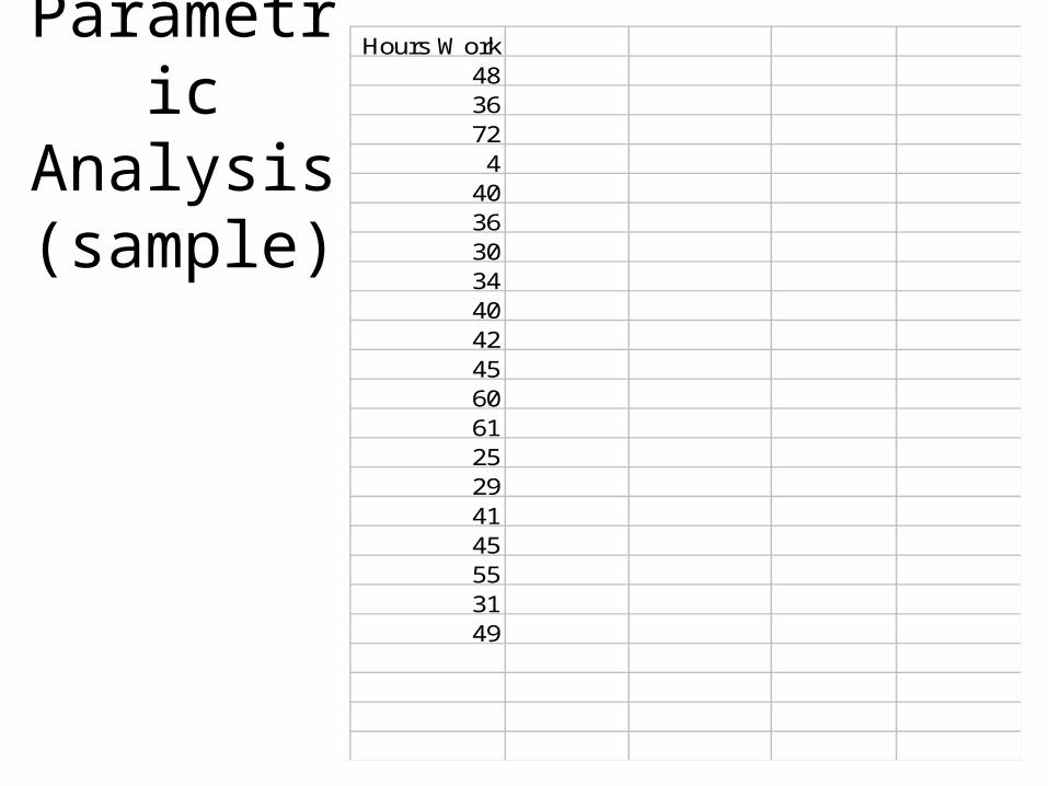
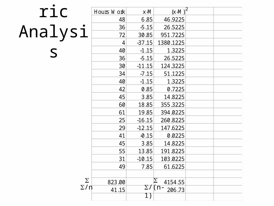
Parametric Analysis (sample)
Hours Work4836724
40363034404245606125294145553149
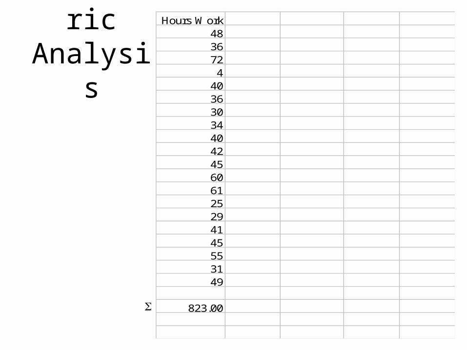
Parametric Analysis
Hours Work4836724
40363034404245606125294145553149
823.00
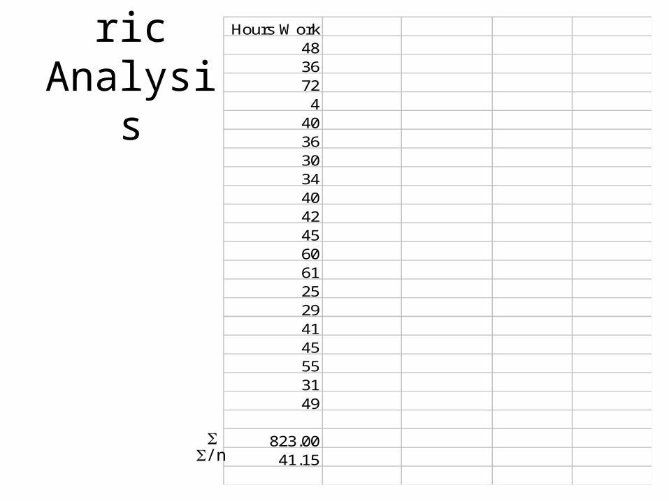
Parametric Analysis
Hours Work4836724
40363034404245606125294145553149
823.0041.15
/n

Parametric Analysis
Hours Work4836724
40363034404245606125294145553149
823.0041.15
/n
M
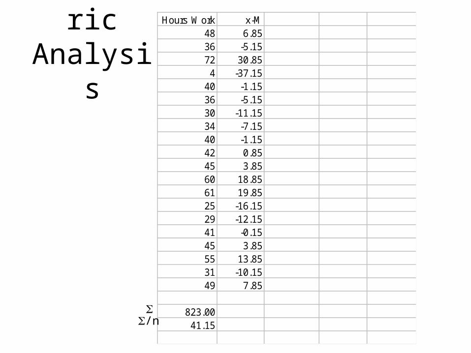
Parametric Analysis
Hours Work x-M48 6.8536 -5.1572 30.85
4 -37.1540 -1.1536 -5.1530 -11.1534 -7.1540 -1.1542 0.8545 3.8560 18.8561 19.8525 -16.1529 -12.1541 -0.1545 3.8555 13.8531 -10.1549 7.85
823.0041.15
/n
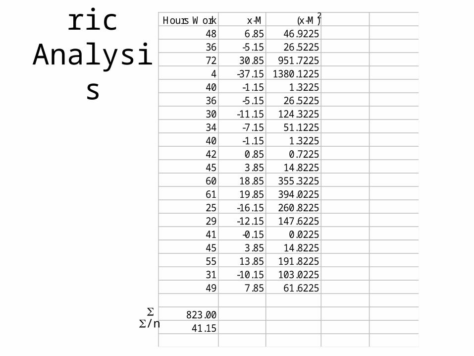
Parametric Analysis
Hours Work x-M (x-M)48 6.85 46.922536 -5.15 26.522572 30.85 951.7225
4 -37.15 1380.122540 -1.15 1.322536 -5.15 26.522530 -11.15 124.322534 -7.15 51.122540 -1.15 1.322542 0.85 0.722545 3.85 14.822560 18.85 355.322561 19.85 394.022525 -16.15 260.822529 -12.15 147.622541 -0.15 0.022545 3.85 14.822555 13.85 191.822531 -10.15 103.022549 7.85 61.6225
823.0041.15
2
/n
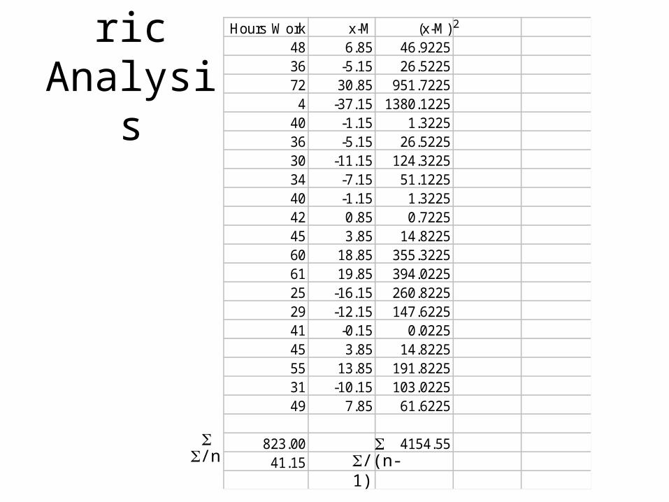
Parametric Analysis
Hours Work x-M (x-M)48 6.85 46.922536 -5.15 26.522572 30.85 951.7225
4 -37.15 1380.122540 -1.15 1.322536 -5.15 26.522530 -11.15 124.322534 -7.15 51.122540 -1.15 1.322542 0.85 0.722545 3.85 14.822560 18.85 355.322561 19.85 394.022525 -16.15 260.822529 -12.15 147.622541 -0.15 0.022545 3.85 14.822555 13.85 191.822531 -10.15 103.022549 7.85 61.6225
823.00 4154.5541.15
2
/n
/(n-1)
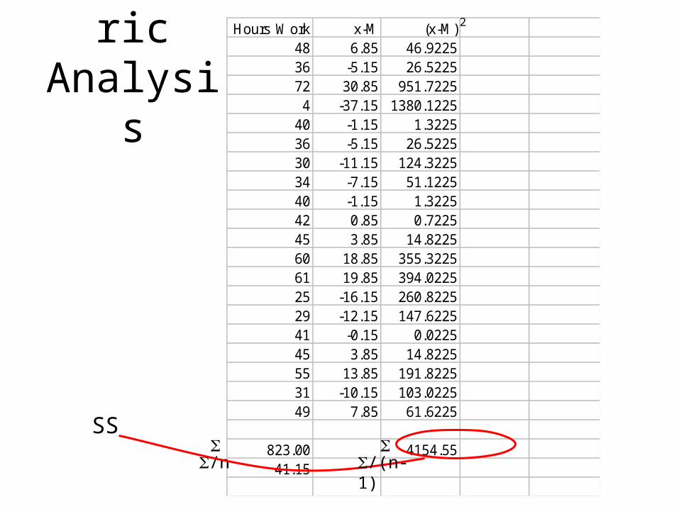
Parametric Analysis
Hours Work x-M (x-M)48 6.85 46.922536 -5.15 26.522572 30.85 951.7225
4 -37.15 1380.122540 -1.15 1.322536 -5.15 26.522530 -11.15 124.322534 -7.15 51.122540 -1.15 1.322542 0.85 0.722545 3.85 14.822560 18.85 355.322561 19.85 394.022525 -16.15 260.822529 -12.15 147.622541 -0.15 0.022545 3.85 14.822555 13.85 191.822531 -10.15 103.022549 7.85 61.6225
823.00 4154.5541.15
2
/n
SS
/(n-1)
Parametric Analysis
Hours Work x-M (x-M)48 6.85 46.922536 -5.15 26.522572 30.85 951.7225
4 -37.15 1380.122540 -1.15 1.322536 -5.15 26.522530 -11.15 124.322534 -7.15 51.122540 -1.15 1.322542 0.85 0.722545 3.85 14.822560 18.85 355.322561 19.85 394.022525 -16.15 260.822529 -12.15 147.622541 -0.15 0.022545 3.85 14.822555 13.85 191.822531 -10.15 103.022549 7.85 61.6225
823.00 4154.5541.15 206.73
2
/n
/(n-1)
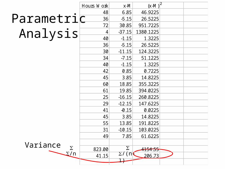
Parametric Analysis
/n
Variance /(n-1)
Hours Work x-M (x-M)48 6.85 46.922536 -5.15 26.522572 30.85 951.7225
4 -37.15 1380.122540 -1.15 1.322536 -5.15 26.522530 -11.15 124.322534 -7.15 51.122540 -1.15 1.322542 0.85 0.722545 3.85 14.822560 18.85 355.322561 19.85 394.022525 -16.15 260.822529 -12.15 147.622541 -0.15 0.022545 3.85 14.822555 13.85 191.822531 -10.15 103.022549 7.85 61.6225
823.00 4154.5541.15 206.73
2
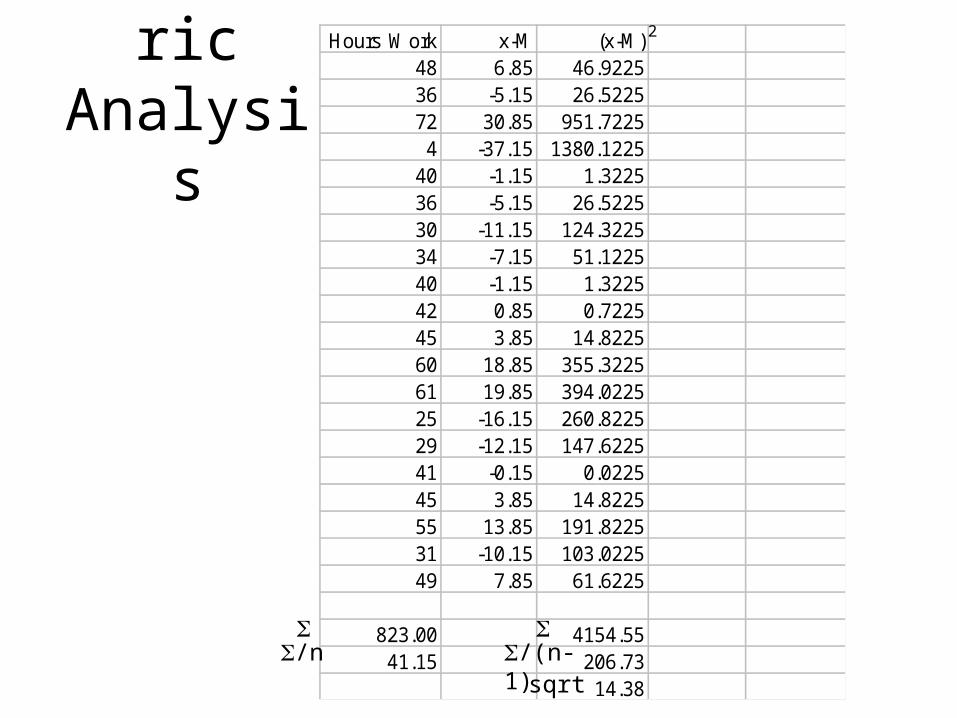
Parametric Analysis
Hours Work x-M (x-M)48 6.85 46.922536 -5.15 26.522572 30.85 951.7225
4 -37.15 1380.122540 -1.15 1.322536 -5.15 26.522530 -11.15 124.322534 -7.15 51.122540 -1.15 1.322542 0.85 0.722545 3.85 14.822560 18.85 355.322561 19.85 394.022525 -16.15 260.822529 -12.15 147.622541 -0.15 0.022545 3.85 14.822555 13.85 191.822531 -10.15 103.022549 7.85 61.6225
823.00 4154.5541.15 206.73
14.38
2
/n
sqrt
/(n-1)
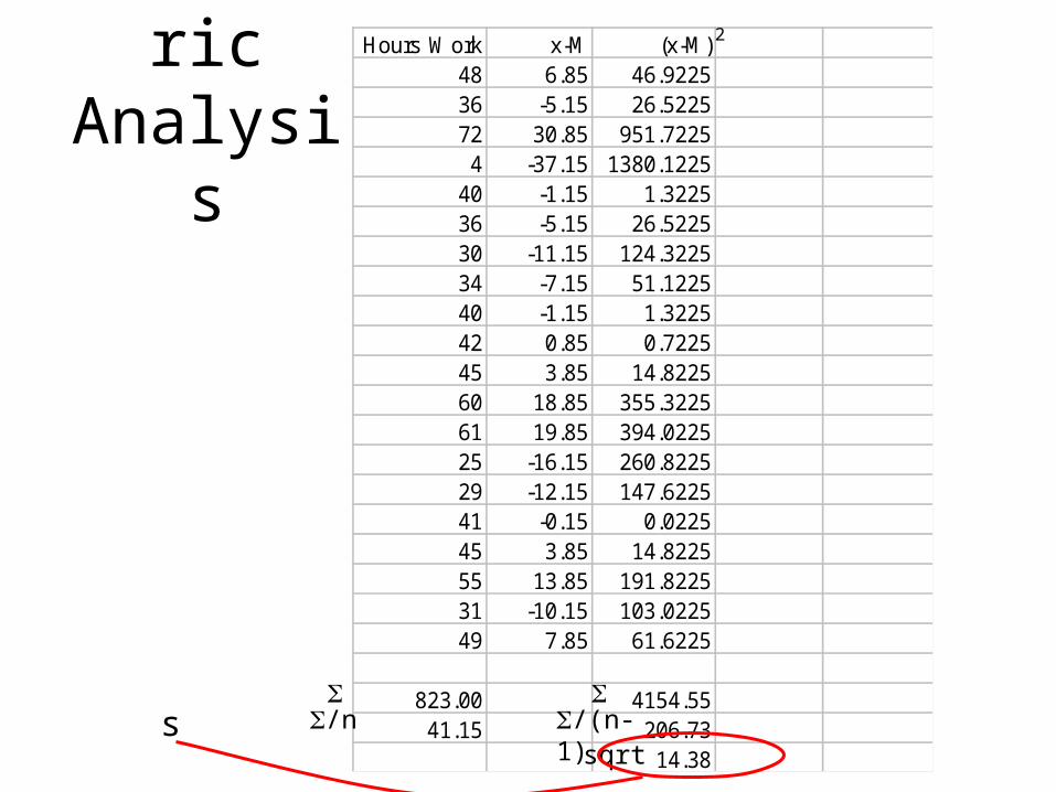
Parametric Analysis
Hours Work x-M (x-M)48 6.85 46.922536 -5.15 26.522572 30.85 951.7225
4 -37.15 1380.122540 -1.15 1.322536 -5.15 26.522530 -11.15 124.322534 -7.15 51.122540 -1.15 1.322542 0.85 0.722545 3.85 14.822560 18.85 355.322561 19.85 394.022525 -16.15 260.822529 -12.15 147.622541 -0.15 0.022545 3.85 14.822555 13.85 191.822531 -10.15 103.022549 7.85 61.6225
823.00 4154.5541.15 206.73
14.38
2
/n
sqrt
/(n-1)s
Parametric Analysis
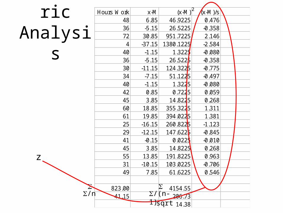
Hours Work x-M (x-M) (x-M)/s48 6.85 46.9225 0.47636 -5.15 26.5225 -0.35872 30.85 951.7225 2.146
4 -37.15 1380.1225 -2.58440 -1.15 1.3225 -0.08036 -5.15 26.5225 -0.35830 -11.15 124.3225 -0.77534 -7.15 51.1225 -0.49740 -1.15 1.3225 -0.08042 0.85 0.7225 0.05945 3.85 14.8225 0.26860 18.85 355.3225 1.31161 19.85 394.0225 1.38125 -16.15 260.8225 -1.12329 -12.15 147.6225 -0.84541 -0.15 0.0225 -0.01045 3.85 14.8225 0.26855 13.85 191.8225 0.96331 -10.15 103.0225 -0.70649 7.85 61.6225 0.546
823.00 4154.5541.15 206.73
14.38
2
/n
sqrt
z
/(n-1)
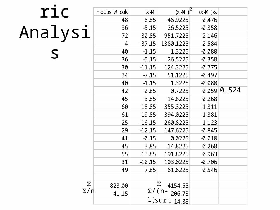
Parametric Analysis
Hours Work x-M (x-M) (x-M)/s48 6.85 46.9225 0.47636 -5.15 26.5225 -0.35872 30.85 951.7225 2.146
4 -37.15 1380.1225 -2.58440 -1.15 1.3225 -0.08036 -5.15 26.5225 -0.35830 -11.15 124.3225 -0.77534 -7.15 51.1225 -0.49740 -1.15 1.3225 -0.08042 0.85 0.7225 0.05945 3.85 14.8225 0.26860 18.85 355.3225 1.31161 19.85 394.0225 1.38125 -16.15 260.8225 -1.12329 -12.15 147.6225 -0.84541 -0.15 0.0225 -0.01045 3.85 14.8225 0.26855 13.85 191.8225 0.96331 -10.15 103.0225 -0.70649 7.85 61.6225 0.546
823.00 4154.5541.15 206.73
14.38
2
/n
sqrt
/(n-1)
0.524

Parametric Analysis
Hours Work x-M (x-M) (x-M)/s48 6.85 46.9225 0.47636 -5.15 26.5225 -0.35872 30.85 951.7225 2.146
4 -37.15 1380.1225 -2.58440 -1.15 1.3225 -0.08036 -5.15 26.5225 -0.35830 -11.15 124.3225 -0.77534 -7.15 51.1225 -0.49740 -1.15 1.3225 -0.08042 0.85 0.7225 0.05945 3.85 14.8225 0.26860 18.85 355.3225 1.31161 19.85 394.0225 1.38125 -16.15 260.8225 -1.12329 -12.15 147.6225 -0.84541 -0.15 0.0225 -0.01045 3.85 14.8225 0.26855 13.85 191.8225 0.96331 -10.15 103.0225 -0.70649 7.85 61.6225 0.546
823.00 4154.5541.15 206.73
14.38
2
/n
sqrt
/(n-1)
0.005
Parametric Analysis
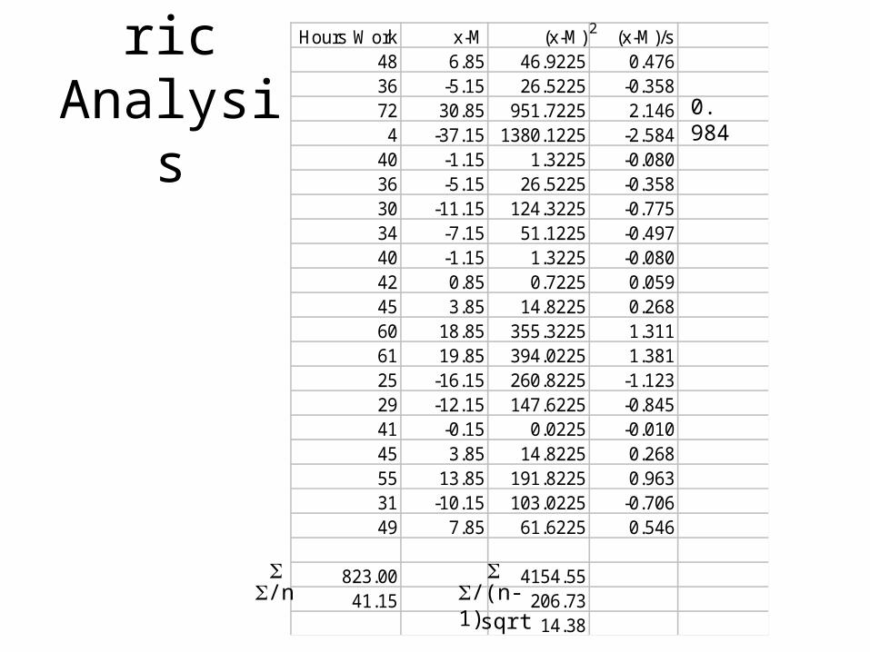
Hours Work x-M (x-M) (x-M)/s48 6.85 46.9225 0.47636 -5.15 26.5225 -0.35872 30.85 951.7225 2.146
4 -37.15 1380.1225 -2.58440 -1.15 1.3225 -0.08036 -5.15 26.5225 -0.35830 -11.15 124.3225 -0.77534 -7.15 51.1225 -0.49740 -1.15 1.3225 -0.08042 0.85 0.7225 0.05945 3.85 14.8225 0.26860 18.85 355.3225 1.31161 19.85 394.0225 1.38125 -16.15 260.8225 -1.12329 -12.15 147.6225 -0.84541 -0.15 0.0225 -0.01045 3.85 14.8225 0.26855 13.85 191.8225 0.96331 -10.15 103.0225 -0.70649 7.85 61.6225 0.546
823.00 4154.5541.15 206.73
14.38
2
/n
sqrt
/(n-1)
0. 984
Parametric Analysis
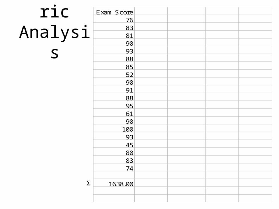
(population)
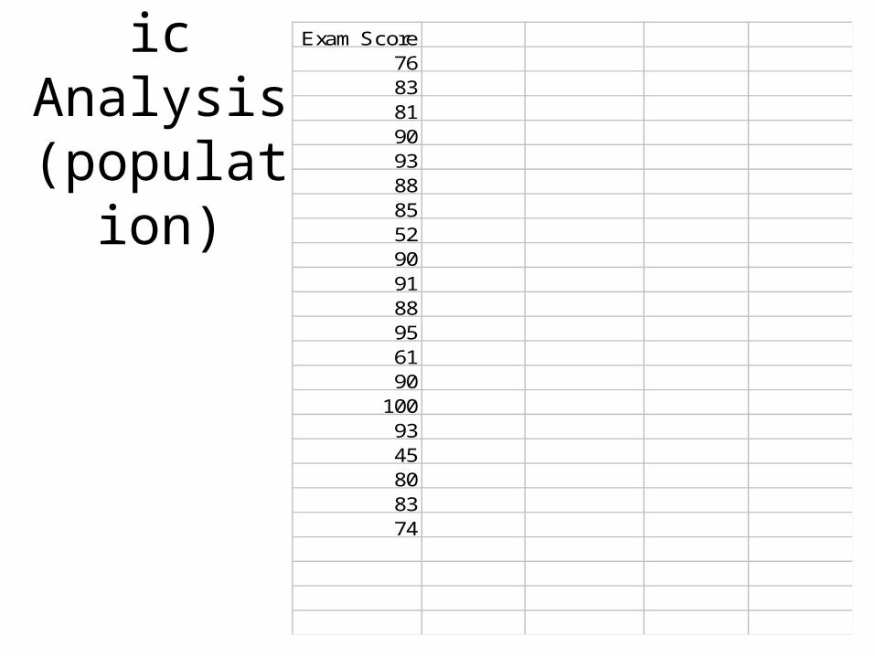
Exam Score7683819093888552909188956190
1009345808374
Parametric Analysis
Exam Score7683819093888552909188956190
1009345808374
1638.00
Parametric Analysis
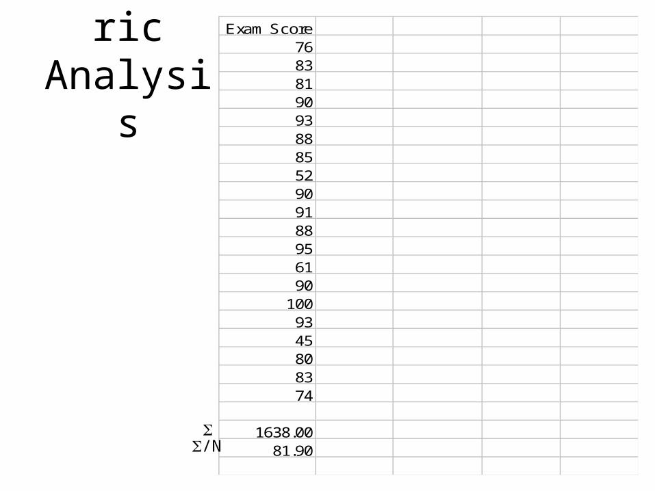
Exam Score7683819093888552909188956190
1009345808374
1638.0081.90
/N
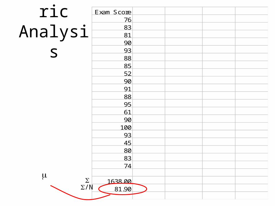
Parametric Analysis
Exam Score7683819093888552909188956190
1009345808374
1638.0081.90
/N
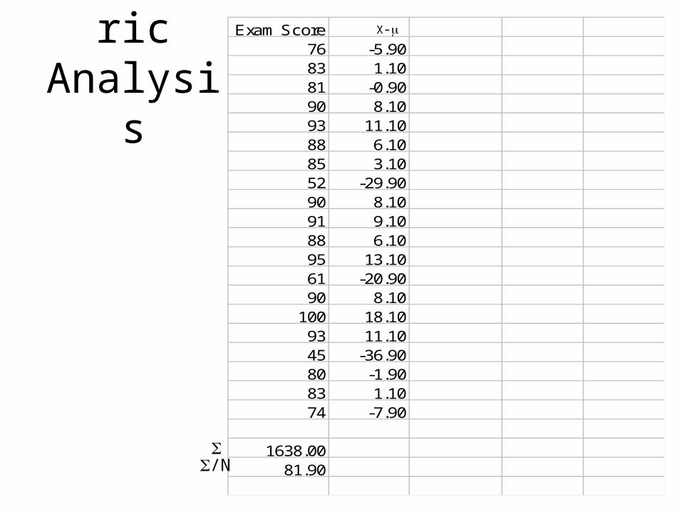
Parametric Analysis
Exam Score76 -5.9083 1.1081 -0.9090 8.1093 11.1088 6.1085 3.1052 -29.9090 8.1091 9.1088 6.1095 13.1061 -20.9090 8.10
100 18.1093 11.1045 -36.9080 -1.9083 1.1074 -7.90
1638.0081.90
/N
X-
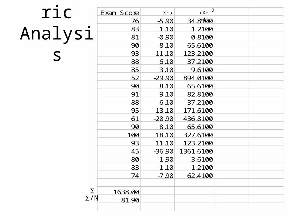
Exam Score76 -5.90 34.810083 1.10 1.210081 -0.90 0.810090 8.10 65.610093 11.10 123.210088 6.10 37.210085 3.10 9.610052 -29.90 894.010090 8.10 65.610091 9.10 82.810088 6.10 37.210095 13.10 171.610061 -20.90 436.810090 8.10 65.6100
100 18.10 327.610093 11.10 123.210045 -36.90 1361.610080 -1.90 3.610083 1.10 1.210074 -7.90 62.4100
1638.0081.90
(X-)Parametric Analysis
/N
X- 2
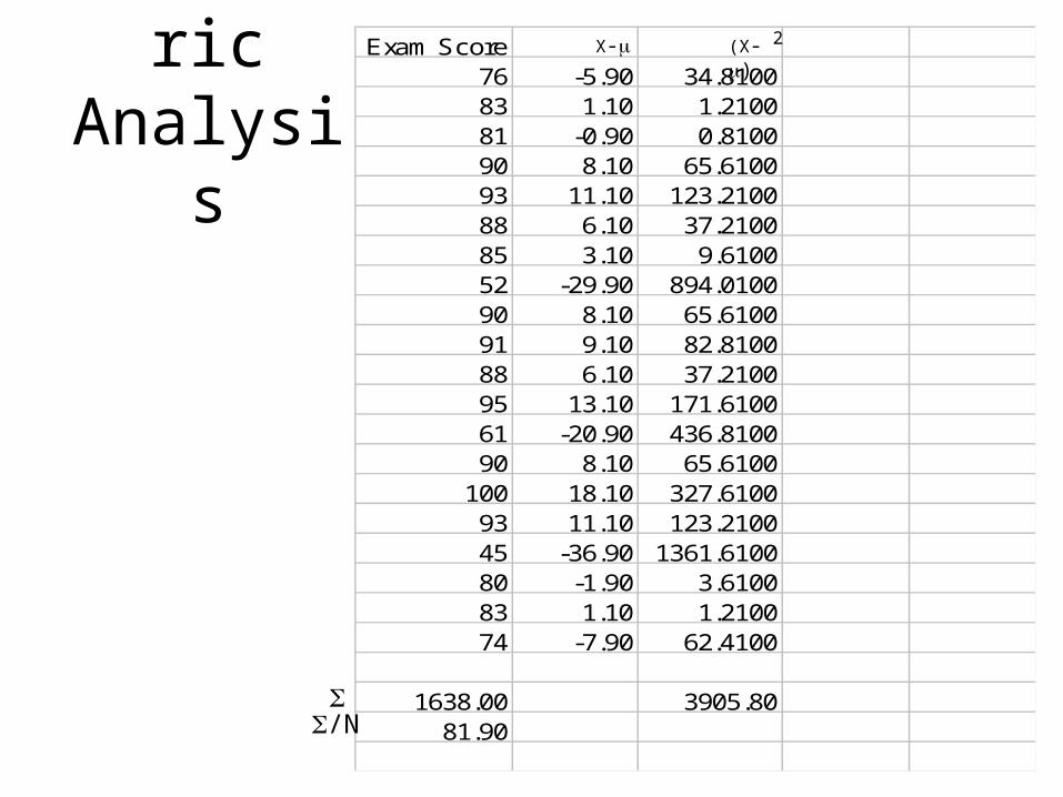
Parametric Analysis
Exam Score76 -5.90 34.810083 1.10 1.210081 -0.90 0.810090 8.10 65.610093 11.10 123.210088 6.10 37.210085 3.10 9.610052 -29.90 894.010090 8.10 65.610091 9.10 82.810088 6.10 37.210095 13.10 171.610061 -20.90 436.810090 8.10 65.6100
100 18.10 327.610093 11.10 123.210045 -36.90 1361.610080 -1.90 3.610083 1.10 1.210074 -7.90 62.4100
1638.00 3905.8081.90
/N
(X-)X- 2
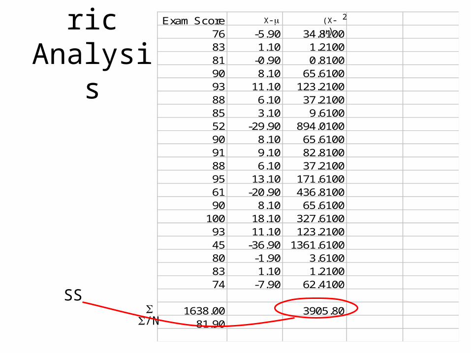
Parametric Analysis
Exam Score76 -5.90 34.810083 1.10 1.210081 -0.90 0.810090 8.10 65.610093 11.10 123.210088 6.10 37.210085 3.10 9.610052 -29.90 894.010090 8.10 65.610091 9.10 82.810088 6.10 37.210095 13.10 171.610061 -20.90 436.810090 8.10 65.6100
100 18.10 327.610093 11.10 123.210045 -36.90 1361.610080 -1.90 3.610083 1.10 1.210074 -7.90 62.4100
1638.00 3905.8081.90
/N
SS
(X-)X- 2
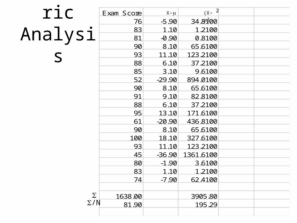
Parametric Analysis
Exam Score76 -5.90 34.810083 1.10 1.210081 -0.90 0.810090 8.10 65.610093 11.10 123.210088 6.10 37.210085 3.10 9.610052 -29.90 894.010090 8.10 65.610091 9.10 82.810088 6.10 37.210095 13.10 171.610061 -20.90 436.810090 8.10 65.6100
100 18.10 327.610093 11.10 123.210045 -36.90 1361.610080 -1.90 3.610083 1.10 1.210074 -7.90 62.4100
1638.00 3905.8081.90 195.29
/N
(X-)X- 2
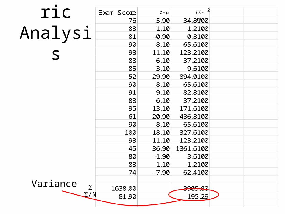
Parametric Analysis
Exam Score76 -5.90 34.810083 1.10 1.210081 -0.90 0.810090 8.10 65.610093 11.10 123.210088 6.10 37.210085 3.10 9.610052 -29.90 894.010090 8.10 65.610091 9.10 82.810088 6.10 37.210095 13.10 171.610061 -20.90 436.810090 8.10 65.6100
100 18.10 327.610093 11.10 123.210045 -36.90 1361.610080 -1.90 3.610083 1.10 1.210074 -7.90 62.4100
1638.00 3905.8081.90 195.29
/N
Variance
(X-)X- 2
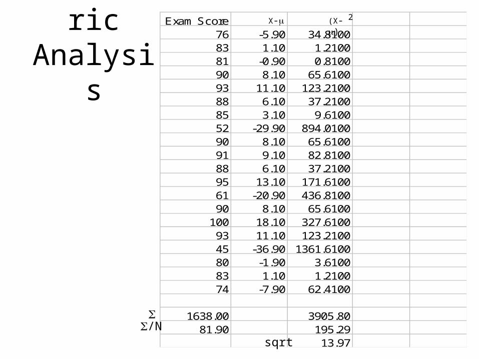
Parametric Analysis
Exam Score76 -5.90 34.810083 1.10 1.210081 -0.90 0.810090 8.10 65.610093 11.10 123.210088 6.10 37.210085 3.10 9.610052 -29.90 894.010090 8.10 65.610091 9.10 82.810088 6.10 37.210095 13.10 171.610061 -20.90 436.810090 8.10 65.6100
100 18.10 327.610093 11.10 123.210045 -36.90 1361.610080 -1.90 3.610083 1.10 1.210074 -7.90 62.4100
1638.00 3905.8081.90 195.29
13.97
/N
sqrt
(X-)X- 2
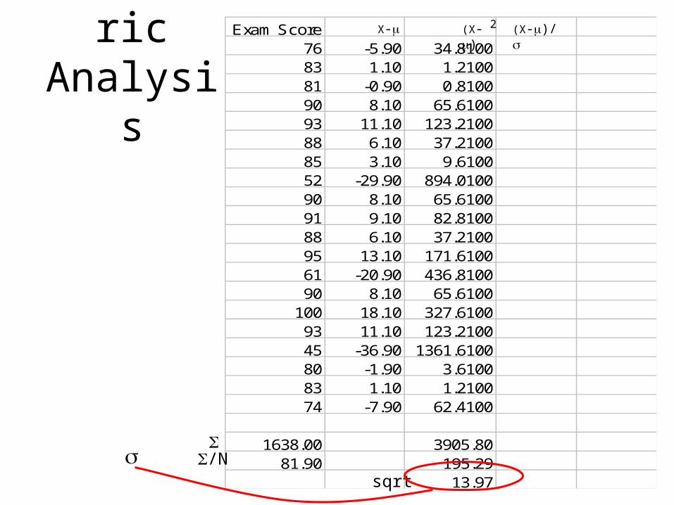
Parametric Analysis
Exam Score76 -5.90 34.810083 1.10 1.210081 -0.90 0.810090 8.10 65.610093 11.10 123.210088 6.10 37.210085 3.10 9.610052 -29.90 894.010090 8.10 65.610091 9.10 82.810088 6.10 37.210095 13.10 171.610061 -20.90 436.810090 8.10 65.6100
100 18.10 327.610093 11.10 123.210045 -36.90 1361.610080 -1.90 3.610083 1.10 1.210074 -7.90 62.4100
1638.00 3905.8081.90 195.29
13.97
/N
sqrt
(X-)X- 2 (X-)/
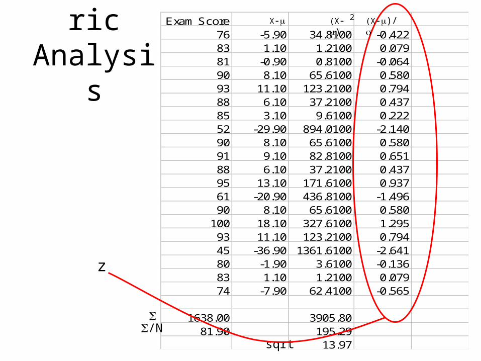
Parametric Analysis
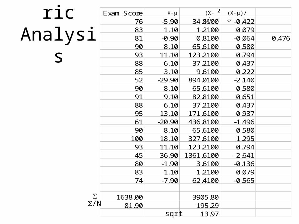
Exam Score76 -5.90 34.8100 -0.42283 1.10 1.2100 0.07981 -0.90 0.8100 -0.06490 8.10 65.6100 0.58093 11.10 123.2100 0.79488 6.10 37.2100 0.43785 3.10 9.6100 0.22252 -29.90 894.0100 -2.14090 8.10 65.6100 0.58091 9.10 82.8100 0.65188 6.10 37.2100 0.43795 13.10 171.6100 0.93761 -20.90 436.8100 -1.49690 8.10 65.6100 0.580
100 18.10 327.6100 1.29593 11.10 123.2100 0.79445 -36.90 1361.6100 -2.64180 -1.90 3.6100 -0.13683 1.10 1.2100 0.07974 -7.90 62.4100 -0.565
1638.00 3905.8081.90 195.29
13.97
/N
sqrt
z
(X-)X- 2 (X-)/
Parametric Analysis
Exam Score76 -5.90 34.8100 -0.42283 1.10 1.2100 0.07981 -0.90 0.8100 -0.064 0.47690 8.10 65.6100 0.58093 11.10 123.2100 0.79488 6.10 37.2100 0.43785 3.10 9.6100 0.22252 -29.90 894.0100 -2.14090 8.10 65.6100 0.58091 9.10 82.8100 0.65188 6.10 37.2100 0.43795 13.10 171.6100 0.93761 -20.90 436.8100 -1.49690 8.10 65.6100 0.580
100 18.10 327.6100 1.29593 11.10 123.2100 0.79445 -36.90 1361.6100 -2.64180 -1.90 3.6100 -0.13683 1.10 1.2100 0.07974 -7.90 62.4100 -0.565
1638.00 3905.8081.90 195.29
13.97
/N
sqrt
(X-)X- 2 (X-)/
Parametric Analysis
Exam Score76 -5.90 34.8100 -0.42283 1.10 1.2100 0.07981 -0.90 0.8100 -0.06490 8.10 65.6100 0.58093 11.10 123.2100 0.79488 6.10 37.2100 0.43785 3.10 9.6100 0.22252 -29.90 894.0100 -2.14090 8.10 65.6100 0.58091 9.10 82.8100 0.65188 6.10 37.2100 0.43795 13.10 171.6100 0.93761 -20.90 436.8100 -1.49690 8.10 65.6100 0.580
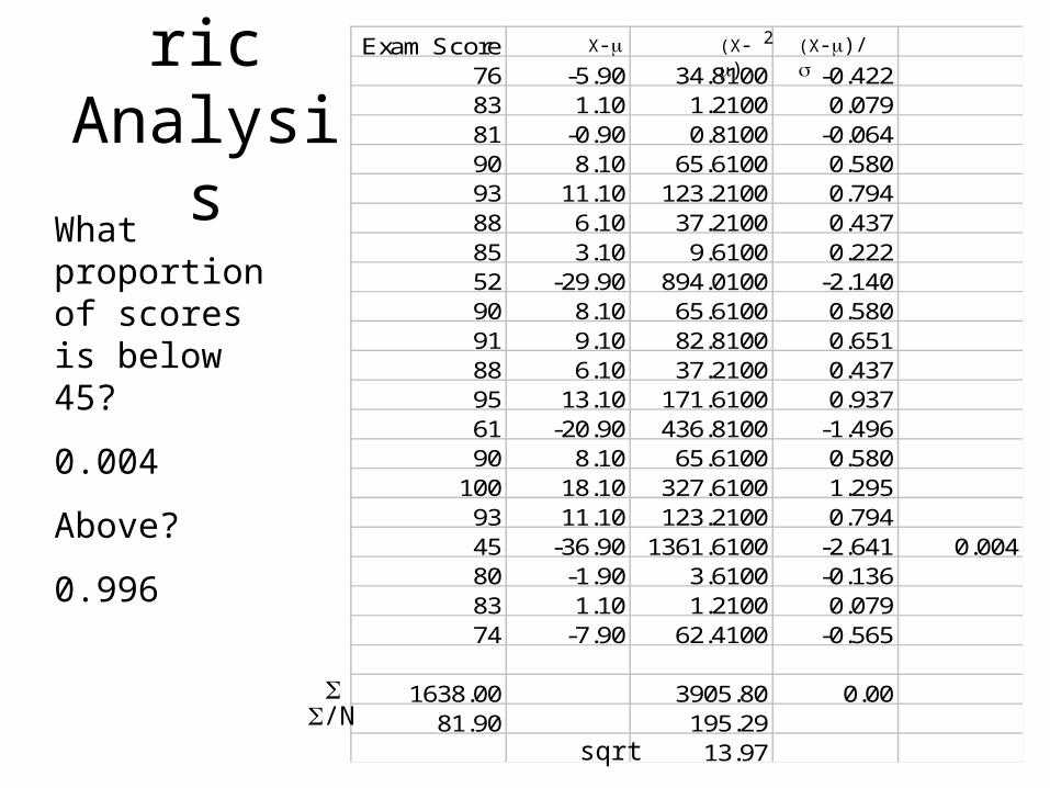
100 18.10 327.6100 1.29593 11.10 123.2100 0.79445 -36.90 1361.6100 -2.641 0.00480 -1.90 3.6100 -0.13683 1.10 1.2100 0.07974 -7.90 62.4100 -0.565
1638.00 3905.80 0.0081.90 195.29
13.97
/N
sqrt
What proportion of scores is below 45?
0.004
Above?
0.996
(X-)X- 2 (X-)/
Parametric Analysis
Exam Score76 -5.90 34.8100 -0.42283 1.10 1.2100 0.07981 -0.90 0.8100 -0.06490 8.10 65.6100 0.58093 11.10 123.2100 0.79488 6.10 37.2100 0.43785 3.10 9.6100 0.22252 -29.90 894.0100 -2.14090 8.10 65.6100 0.58091 9.10 82.8100 0.65188 6.10 37.2100 0.43795 13.10 171.6100 0.93761 -20.90 436.8100 -1.49690 8.10 65.6100 0.580
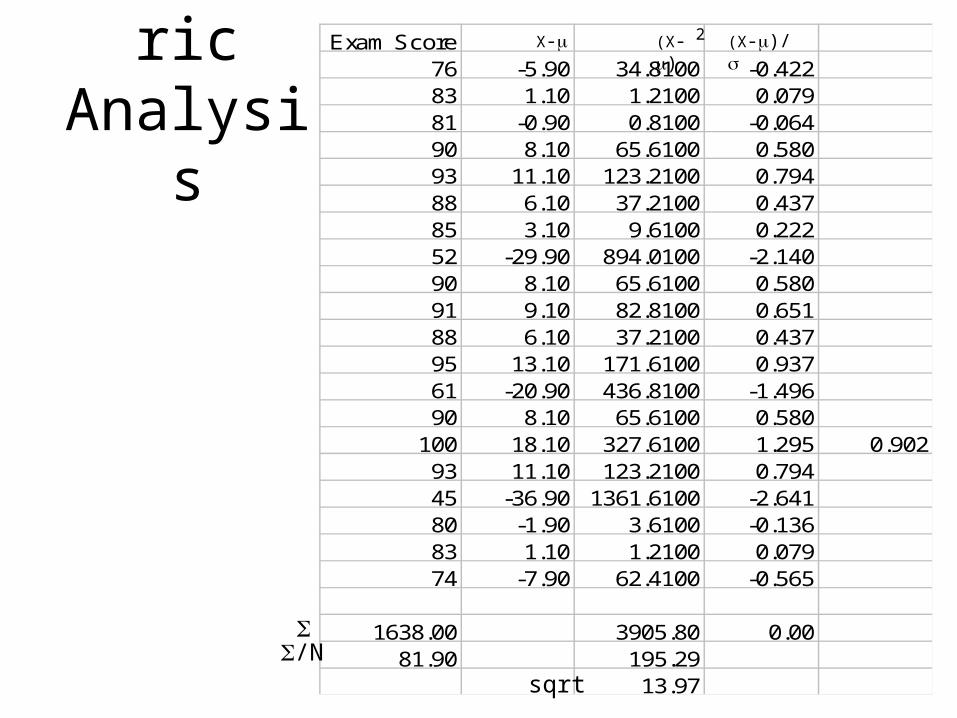
100 18.10 327.6100 1.295 0.90293 11.10 123.2100 0.79445 -36.90 1361.6100 -2.64180 -1.90 3.6100 -0.13683 1.10 1.2100 0.07974 -7.90 62.4100 -0.565
1638.00 3905.80 0.0081.90 195.29
13.97
/N
sqrt
(X-)X- 2 (X-)/
Parametric Analysis
Exam Score76 -5.90 34.8100 -0.42283 1.10 1.2100 0.07981 -0.90 0.8100 -0.06490 8.10 65.6100 0.58093 11.10 123.2100 0.79488 6.10 37.2100 0.43785 3.10 9.6100 0.22252 -29.90 894.0100 -2.14090 8.10 65.6100 0.58091 9.10 82.8100 0.65188 6.10 37.2100 0.43795 13.10 171.6100 0.93761 -20.90 436.8100 -1.49690 8.10 65.6100 0.580
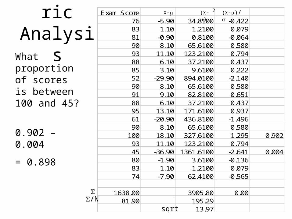
100 18.10 327.6100 1.295 0.90293 11.10 123.2100 0.79445 -36.90 1361.6100 -2.641 0.00480 -1.90 3.6100 -0.13683 1.10 1.2100 0.07974 -7.90 62.4100 -0.565
1638.00 3905.80 0.0081.90 195.29
13.97
/N
sqrt
What proportion of scores is between 100 and 45?
0.902 – 0.004
= 0.898
(X-)X- 2 (X-)/
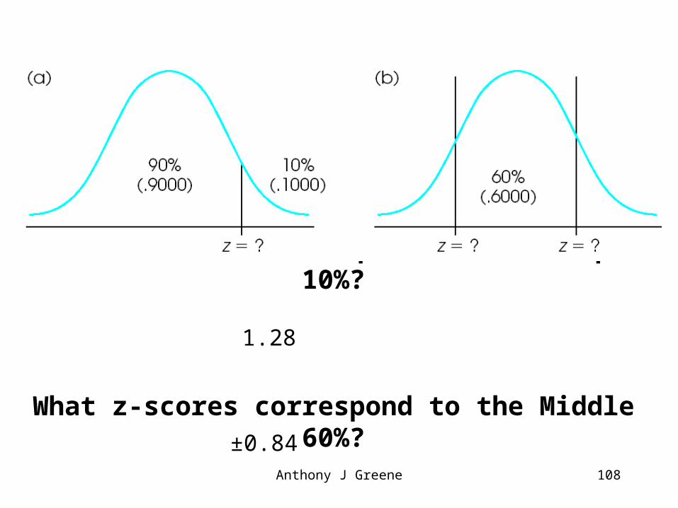
Anthony J Greene 108
What z-score corresponds to the Top 10%?
What z-scores correspond to the Middle 60%?
1.28
±0.84
Anthony J Greene 109
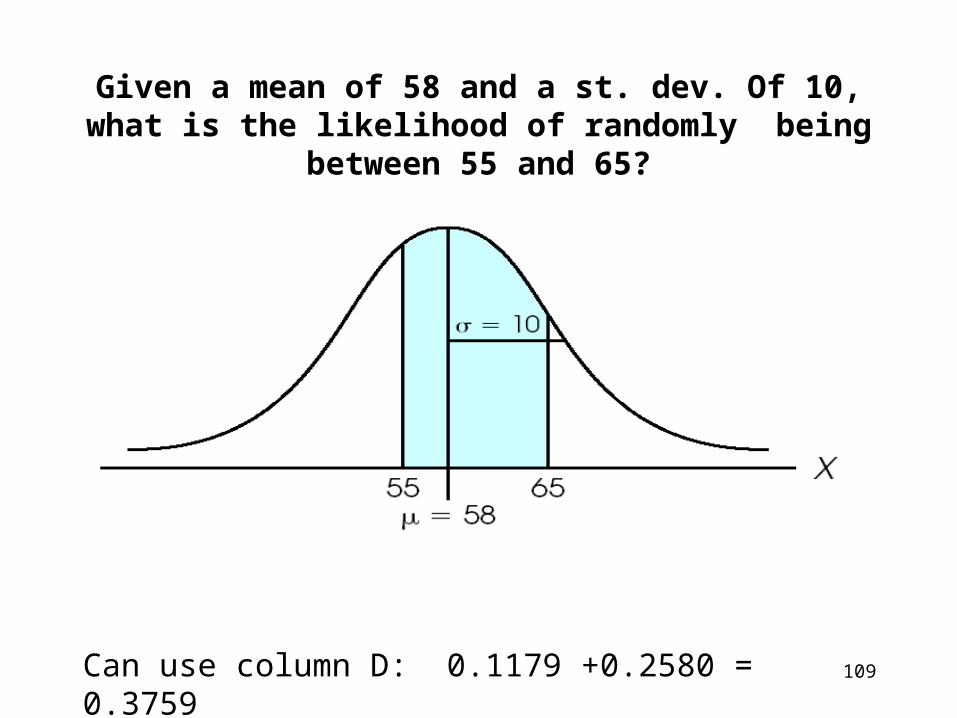
Given a mean of 58 and a st. dev. Of 10, what is the likelihood of randomly being between 55 and 65?
Can use column D: 0.1179 +0.2580 = 0.3759
Anthony J Greene 110
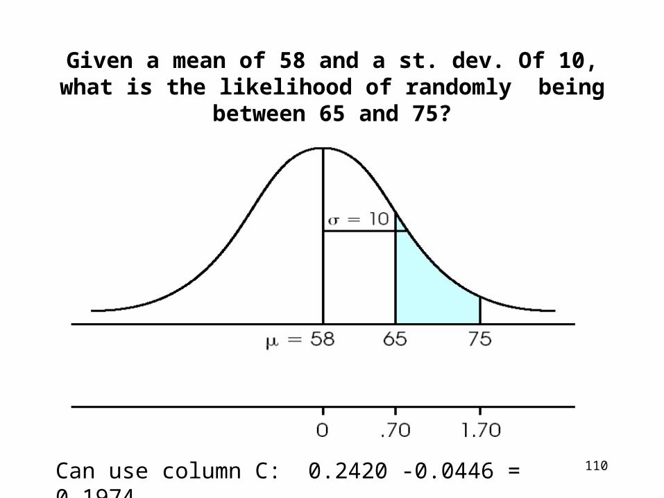
Given a mean of 58 and a st. dev. Of 10, what is the likelihood of randomly being between 65 and 75?
Can use column C: 0.2420 -0.0446 = 0.1974
Anthony J Greene 111
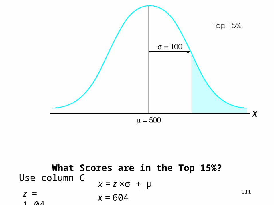
What Scores are in the Top 15%?
z = 1.04
Use column Cx = z ×σ + μ
x = 604
Anthony J Greene 112
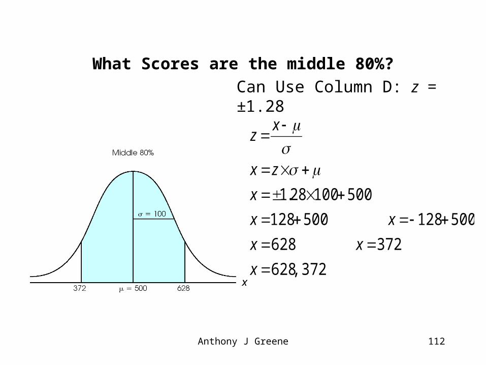
What Scores are the middle 80%?
Can Use Column D: z = ±1.28
372 ,628
372 628
500128 500128
50010028.1
x
xx
xx
x
zx
xz
Anthony J Greene 113
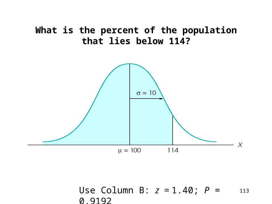
What is the percent of the population that lies below 114?
Use Column B: z = 1.40; P = 0.9192
Anthony J Greene 114
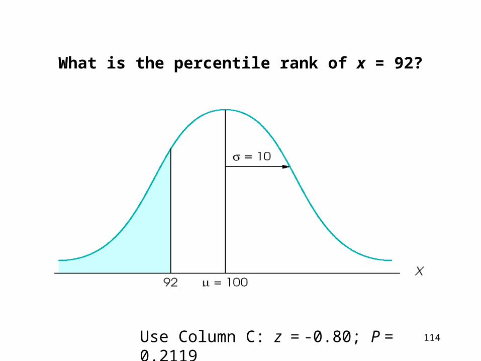
What is the percentile rank of x = 92?
Use Column C: z = -0.80; P = 0.2119
Anthony J Greene 115
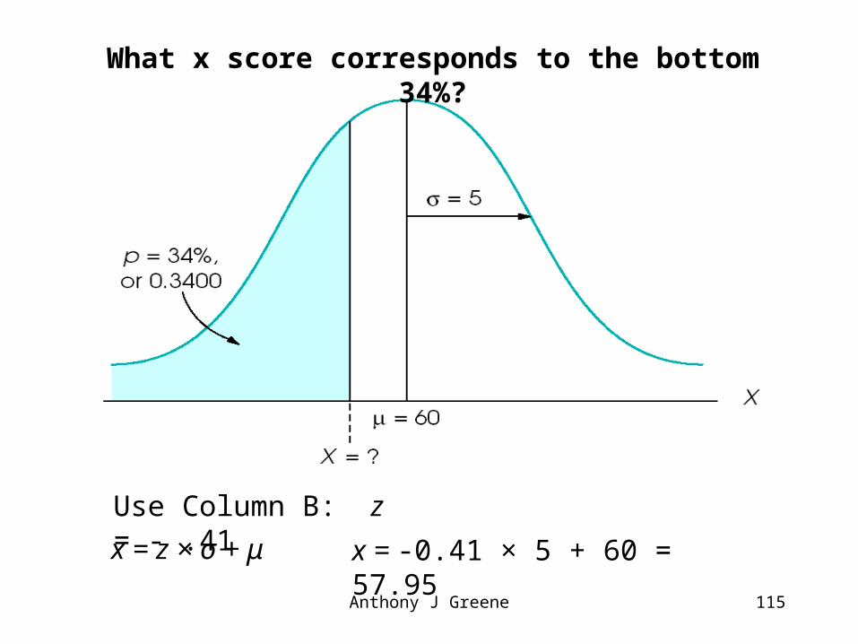
What x score corresponds to the bottom 34%?
Use Column B: z = - .41
x = z × σ + μ x = -0.41 × 5 + 60 = 57.95