Embed Size (px)
Citation preview
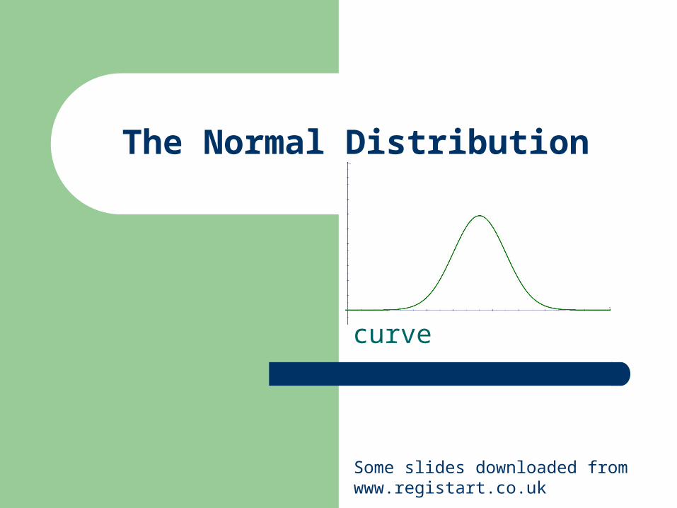
The Normal Distribution
“the bell curve”
Some slides downloaded from www.registart.co.uk

The Most Important Distribution in Statistics!
Describes the characteristics of many real-world data sets:– test scores for large groups of students– actual sizes (length, width) of jeans at Kohl’s– eyesight of all 20-year-olds in Kissimmee– actual lifetimes of 1000 AA batteries– testosterone level of all male students at GHS– length of middle finger of 250 students
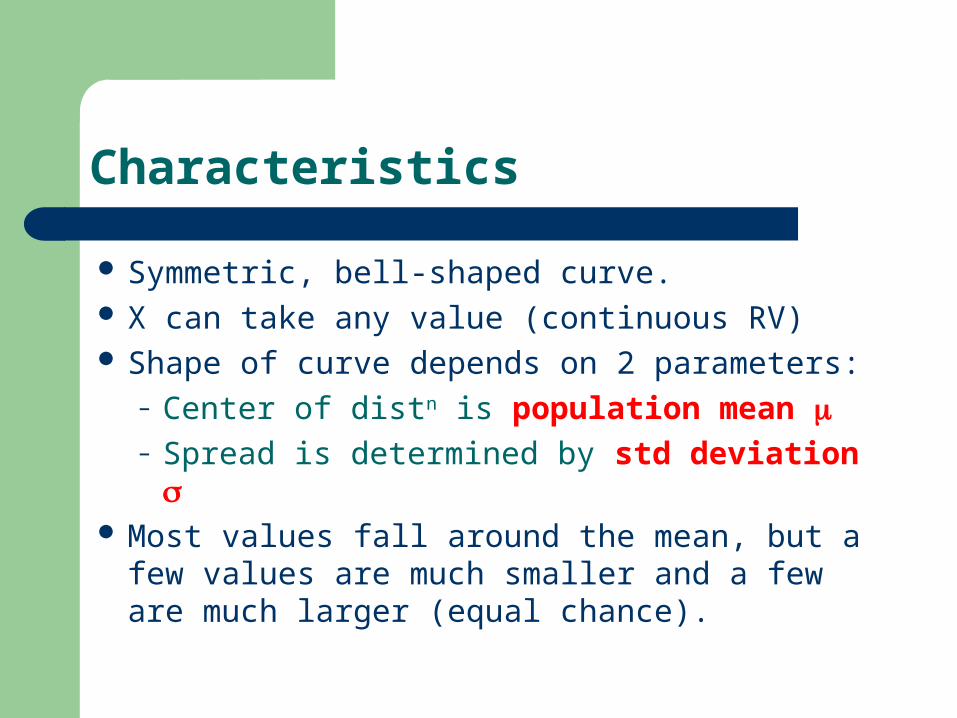
Characteristics
Symmetric, bell-shaped curve. X can take any value (continuous RV) Shape of curve depends on 2 parameters:
– Center of distn is population mean – Spread is determined by std deviation
Most values fall around the mean, but a few values are much smaller and a few are much larger (equal chance).
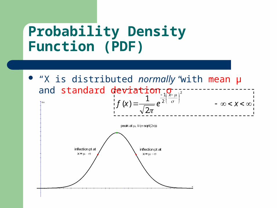
Probability Density Function (PDF)
“X is distributed normally with mean μ and standard deviation σ”
xexfx
2
2
1
2
1)(

Shape Depends on Mean, Std. Dev
40 50 60 70 80 90 100
0.00
0.01
0.02
0.03
0.04
0.05
0.06
0.07
0.08
Grades
Den
sity
Bell-shaped curve
Mean = 70 SD = 5
Mean = 70 SD = 10

As a Histogram(Area of rectangle = probability)
Symmetrical Binomial Distribution B(10, 0.5)
0
0.05
0.1
0.15
0.2
0.25
0.3
0 1 2 3 4 5 6 7 8 9 10
r
Pro
b
P(X=r)

Decrease interval size...Symmetrical Binomial Distribution
B(30, 0.5)
0
0.02
0.04
0.06
0.08
0.1
0.12
0.14
0.16
0 1 2 3 4 5 6 7 8 9 10 11 12 13 14 15 16 17 18 19 20 21 22 23 24 25 26 27 28 29 30
r
Pro
b
P(X=r)
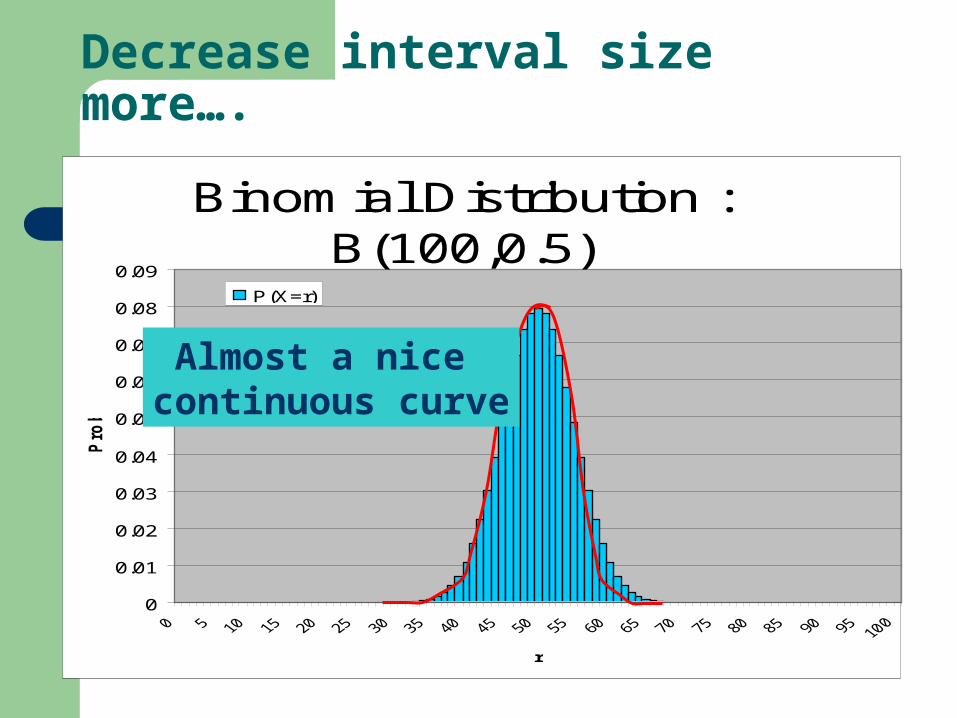
Decrease interval size more….
Binomial Distribution : B(100,0.5)
0
0.01
0.02
0.03
0.04
0.05
0.06
0.07
0.08
0.09
r
Pro
b
P(X=r)
Almost a nice continuous curve
Probability = Area under Curve
Curve describes probability of getting a range of values– e.g., P(X > 60), P(X < 30), P(20 < X < 50)
Area under whole curve = 1 Probability of getting specific number is 0, e.g. P(X=60) = 0
– so P(x < 60) is the same as P(x ≤ 60)
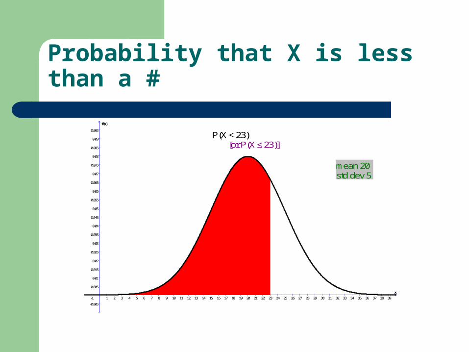
Probability that X is less than a #
-1 1 2 3 4 5 6 7 8 9 10 11 12 13 14 15 16 17 18 19 20 21 22 23 24 25 26 27 28 29 30 31 32 33 34 35 36 37 38 39
-0.005
0.005
0.01
0.015
0.02
0.025
0.03
0.035
0.04
0.045
0.05
0.055
0.06
0.065
0.07
0.075
0.08
0.085
0.09
0.095
x
f(x)
P(X < 23) [or P(X ≤ 23)]
mean 20std dev 5
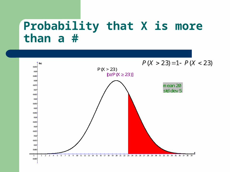
Probability that X is more than a #
-1 1 2 3 4 5 6 7 8 9 10 11 12 13 14 15 16 17 18 19 20 21 22 23 24 25 26 27 28 29 30 31 32 33 34 35 36 37 38 39
-0.005
0.005
0.01
0.015
0.02
0.025
0.03
0.035
0.04
0.045
0.05
0.055
0.06
0.065
0.07
0.075
0.08
0.085
0.09
0.095
x
f(x)
P(X > 23) [or P(X ≥ 23)]
mean 20std dev 5
)23(1)23( XPXP
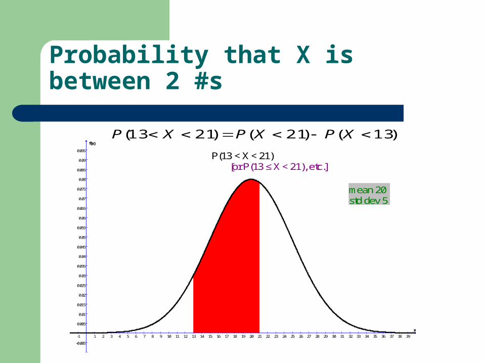
Probability that X is between 2 #s
-1 1 2 3 4 5 6 7 8 9 10 11 12 13 14 15 16 17 18 19 20 21 22 23 24 25 26 27 28 29 30 31 32 33 34 35 36 37 38 39
-0.005
0.005
0.01
0.015
0.02
0.025
0.03
0.035
0.04
0.045
0.05
0.055
0.06
0.065
0.07
0.075
0.08
0.085
0.09
0.095
x
f(x)
P(13 < X < 21) [or P(13 ≤ X < 21), etc.]
mean 20std dev 5
)13()21()2113( XPXPXP
Standard Deviation
Graph (H&H p.730)
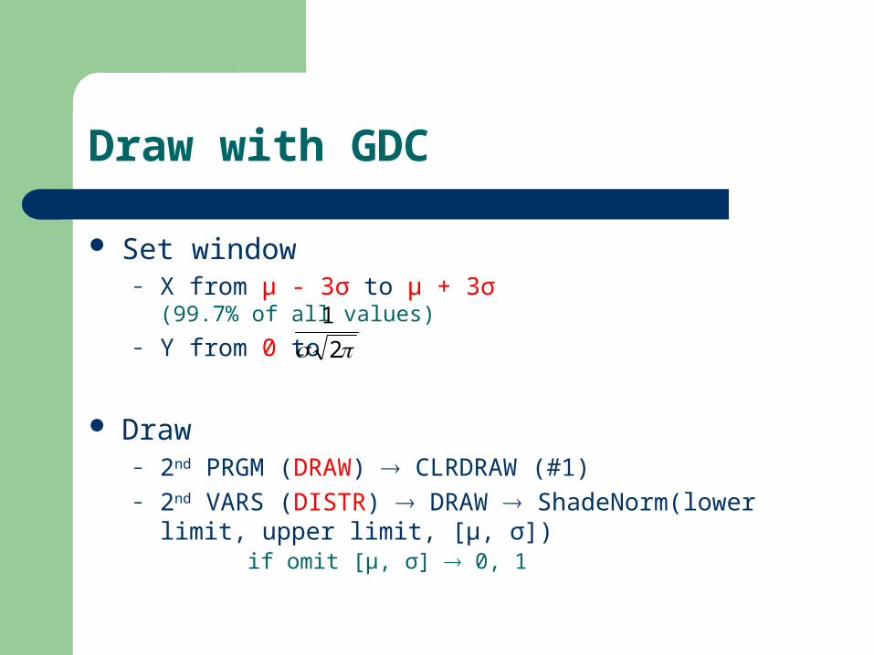
Draw with GDC
Set window– X from μ - 3σ to μ + 3σ (99.7% of all values)
– Y from 0 to
Draw– 2nd PRGM (DRAW) CLRDRAW (#1)– 2nd VARS (DISTR) DRAW ShadeNorm(lower limit,
upper limit, [μ, σ]) if omit [μ, σ] 0, 1
2
1

Draw with GDC (con’t)
For normally distributed X with mean 15, std dev 2:
P(8 ≤ X ≤ 12): use ShadeNorm(8, 12, 15, 2) P(X ≥ 17): use ShadeNorm(17, E99, 15, 2) P(X ≤ 16): use ShadeNorm(-E99, 16, 15,
2)
use E99 in place of ∞, -E99 in place of -∞
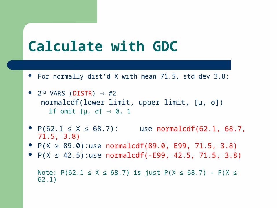
Calculate with GDC
For normally dist’d X with mean 71.5, std dev 3.8:
2nd VARS (DISTR) #2
normalcdf(lower limit, upper limit, [μ, σ])if omit [μ, σ] 0, 1
P(62.1 ≤ X ≤ 68.7): use normalcdf(62.1, 68.7, 71.5, 3.8) P(X ≥ 89.0): use normalcdf(89.0, E99, 71.5, 3.8) P(X ≤ 42.5): use normalcdf(-E99, 42.5, 71.5, 3.8)
Note: P(62.1 ≤ X ≤ 68.7) is just P(X ≤ 68.7) - P(X ≤ 62.1)
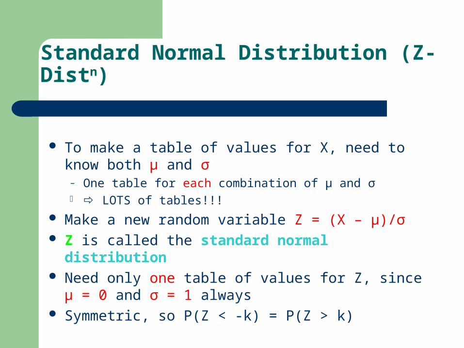
Standard Normal Distribution (Z-Distn)
To make a table of values for X, need to know both μ and σ
– One table for each combination of μ and σ LOTS of tables!!!
Make a new random variable Z = (X – μ)/σ Z is called the standard normal distribution Need only one table of values for Z, since μ = 0 and
σ = 1 always Symmetric, so P(Z < -k) = P(Z > k)
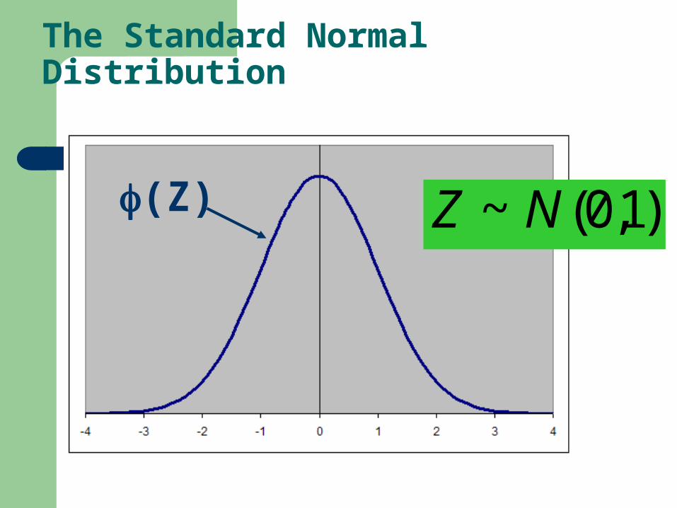
The Standard Normal Distribution
)1,0(~ NZ(Z)

Z-Values (“Z-Scores”)
Value of Z is just the # of standard deviations from the mean:– Z = -2 corresponds to X = μ - 2σ– Z = -1 corresponds to X = μ - σ– Z = 0 corresponds to X = μ– Z = 1 corresponds to X = μ + σ– Z = 2 corresponds to X = μ + 2σ
Etc.
(Insert graph of preceding slide)
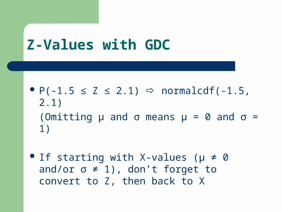
Z-Values with GDC
P(-1.5 ≤ Z ≤ 2.1) normalcdf(-1.5, 2.1)
(Omitting μ and σ means μ = 0 and σ = 1)
If starting with X-values (μ ≠ 0 and/or σ ≠ 1), don’t forget to convert to Z, then back to X
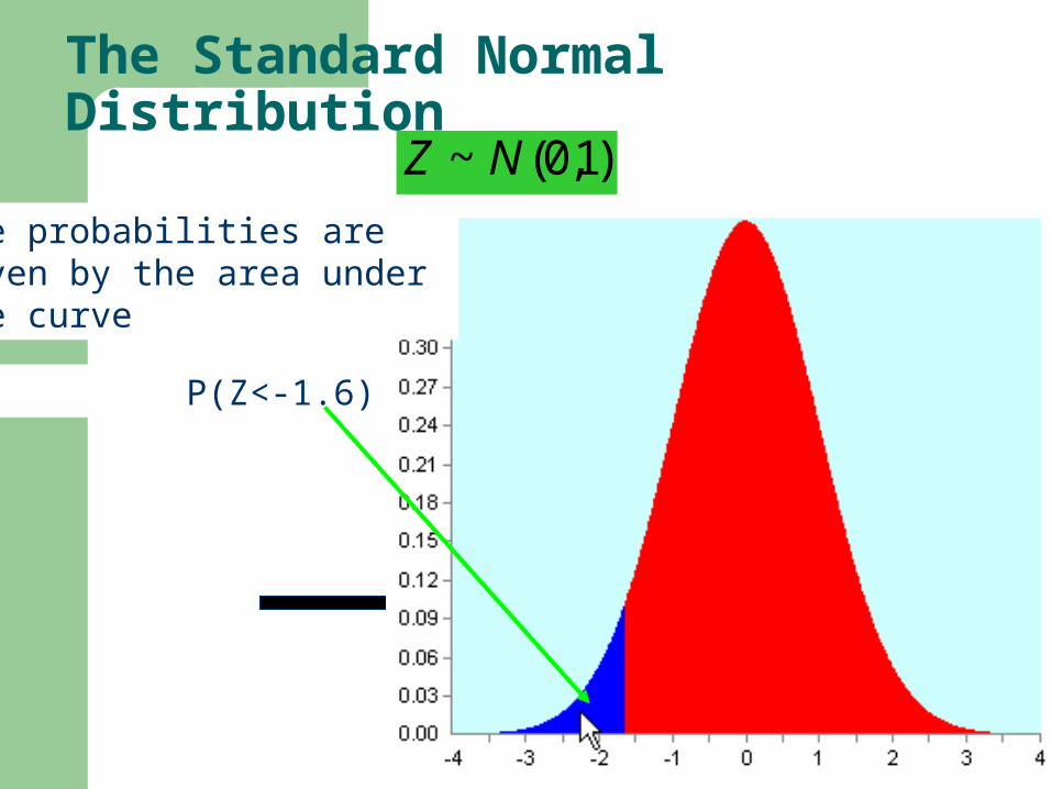
The Standard Normal Distribution)1,0(~ NZ
The probabilities are given by the area under the curve
P(Z<-1.6)
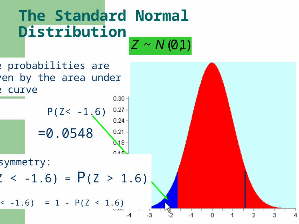
The Standard Normal Distribution)1,0(~ NZ
The probabilities are given by the area under the curve
P(Z< -1.6)
=0.0548
By symmetry:
P(Z < -1.6) = P(Z > 1.6) P(Z < -1.6) = 1 - P(Z < 1.6)
Z-Values from Tables
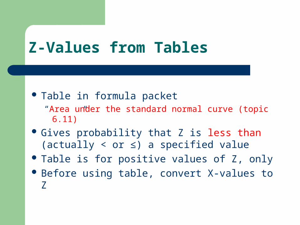
Table in formula packet“Area under the standard normal curve (topic 6.11)”
Gives probability that Z is less than (actually < or ≤) a specified value
Table is for positive values of Z, only Before using table, convert X-values to Z

Reading Table of Z-Values
(INSERT picture of table), with animations showing how to read z to 2 decimal places
Highlight Z-values on top and on left, highlight cross-indexed area

Example : Using Table of Z-Values
For X with mean μ = 26, std dev σ = 1.4,find P(X < 27.1)
Z = (X – μ)/σ = (27.1 – 26)/1.4 = 0.786 use Z = 0.79
P(X < 27.1) = P(Z < 0.79) = 0.7852
compare to answer from normalcdf(-E99, 27.1, 26, 1.4) P(X < 27.1) = 0.7840 (slightly different because we rounded Z)
P(X < 27.106) = P(Z < 0.79) (no rounding) = 0.7852 (to 4 d.p.’s)

Extending the Table
Table from formula packet only works for:– P(Z < z)– Positive Z-values
What to do if you want P(Z > z), or if Z is a negative value?
Think of the graph and which areas you should shade…
Calculating P(Z > z) from Table
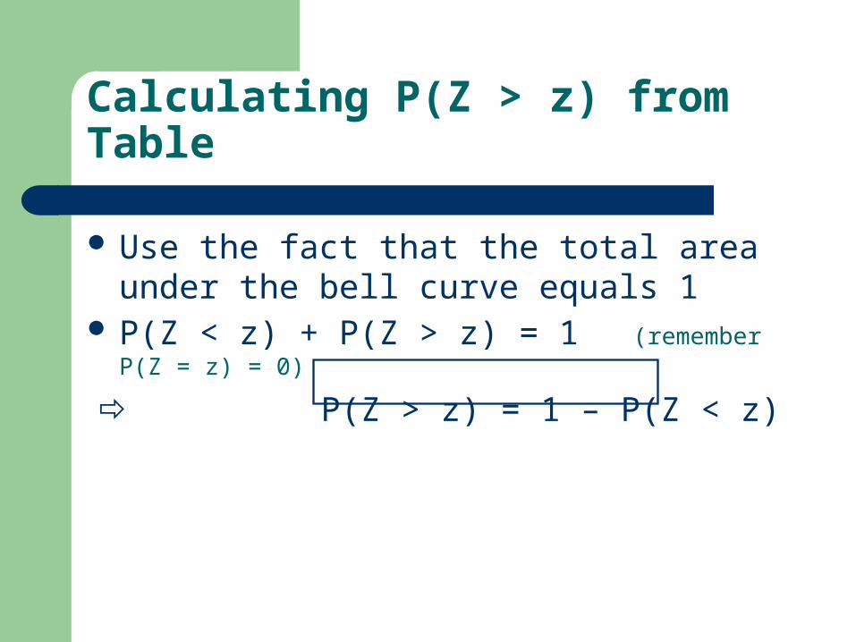
Use the fact that the total area under the bell curve equals 1
P(Z < z) + P(Z > z) = 1 (remember P(Z = z) = 0)
P(Z > z) = 1 – P(Z < z)
Example: P(Z > z) from Table
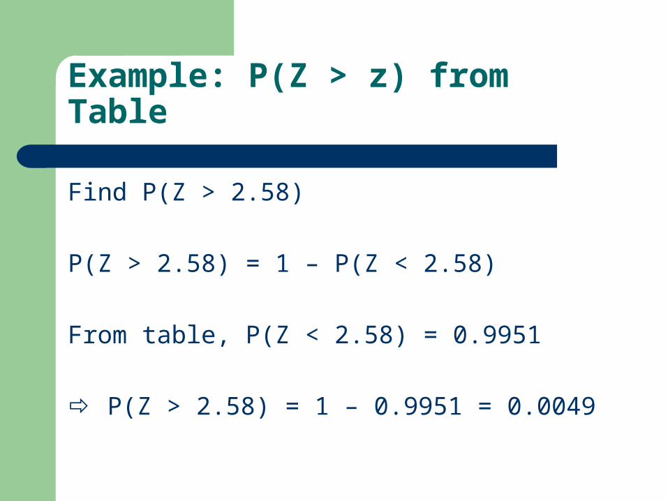
Find P(Z > 2.58)
P(Z > 2.58) = 1 – P(Z < 2.58)
From table, P(Z < 2.58) = 0.9951
P(Z > 2.58) = 1 – 0.9951 = 0.0049
Example: P(X > x)
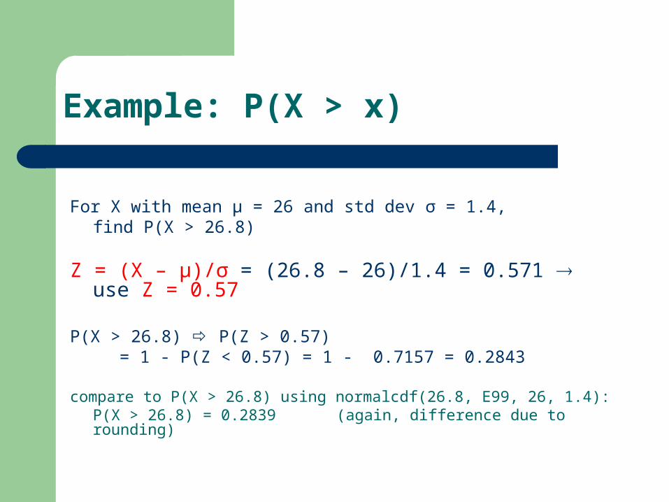
For X with mean μ = 26 and std dev σ = 1.4,find P(X > 26.8)
Z = (X – μ)/σ = (26.8 – 26)/1.4 = 0.571 use Z = 0.57
P(X > 26.8) P(Z > 0.57)= 1 - P(Z < 0.57) = 1 - 0.7157 =
0.2843
compare to P(X > 26.8) using normalcdf(26.8, E99, 26, 1.4):P(X > 26.8) = 0.2839 (again, difference due to rounding)
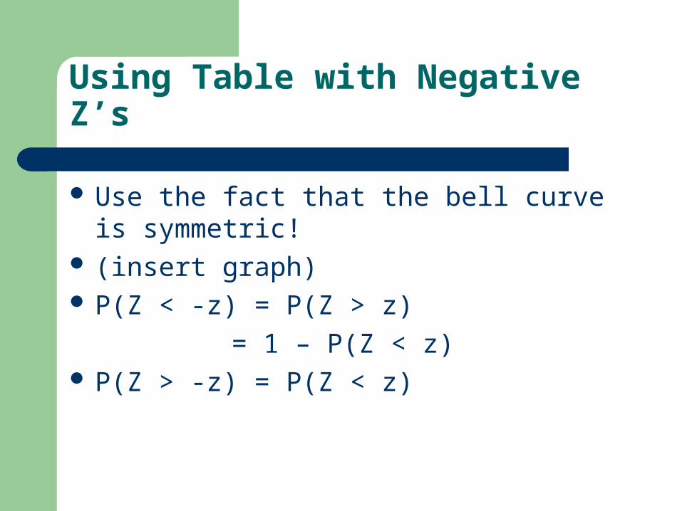
Using Table with Negative Z’s
Use the fact that the bell curve is symmetric! (insert graph) P(Z < -z) = P(Z > z)
= 1 – P(Z < z) P(Z > -z) = P(Z < z)
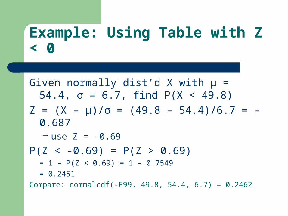
Example: Using Table with Z < 0
Given normally dist’d X with μ = 54.4, σ = 6.7, find P(X < 49.8)
Z = (X – μ)/σ = (49.8 – 54.4)/6.7 = -0.687 use Z = -0.69
P(Z < -0.69) = P(Z > 0.69)= 1 – P(Z < 0.69) = 1 – 0.7549
= 0.2451
Compare: normalcdf(-E99, 49.8, 54.4, 6.7) = 0.2462
Using Table for P(a < X < b)
Subtract the areas P(a < X < b) = P(X < b) – P(X < a) INSERT pictures
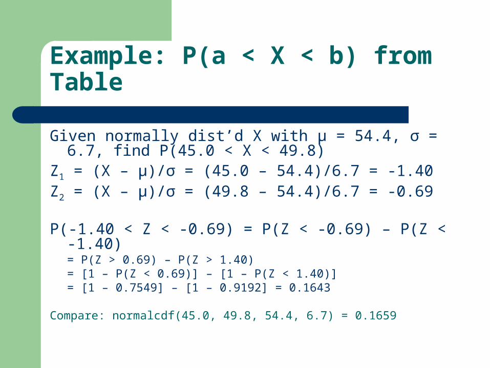
Example: P(a < X < b) from Table
Given normally dist’d X with μ = 54.4, σ = 6.7, find P(45.0 < X < 49.8)
Z1 = (X – μ)/σ = (45.0 – 54.4)/6.7 = -1.40Z2 = (X – μ)/σ = (49.8 – 54.4)/6.7 = -0.69
P(-1.40 < Z < -0.69) = P(Z < -0.69) – P(Z < -1.40)= P(Z > 0.69) – P(Z > 1.40)= [1 – P(Z < 0.69)] – [1 – P(Z < 1.40)]= [1 – 0.7549] – [1 – 0.9192] = 0.1643
Compare: normalcdf(45.0, 49.8, 54.4, 6.7) = 0.1659

Inverse Normal Probabilities
Now we work backwards:– know the probability– want to find corresponding value of X (or Z)
Examples of questions:– Find k such that P(X ≤ k) = 95.4%– If P(-0.10 < X < b) = 0.357 (i.e., 35.7%), find b– Find μ so that P(X > 0.771) = 80.8%
Could use trial and error, but there’s a better way
Inverse Normal Probabilities by GDC
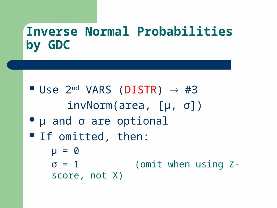
Use 2nd VARS (DISTR) #3
invNorm(area, [μ, σ]) μ and σ are optional If omitted, then:
μ = 0
σ = 1 (omit when using Z-score, not X)
Example: Inv. Normal Prob. by GDC
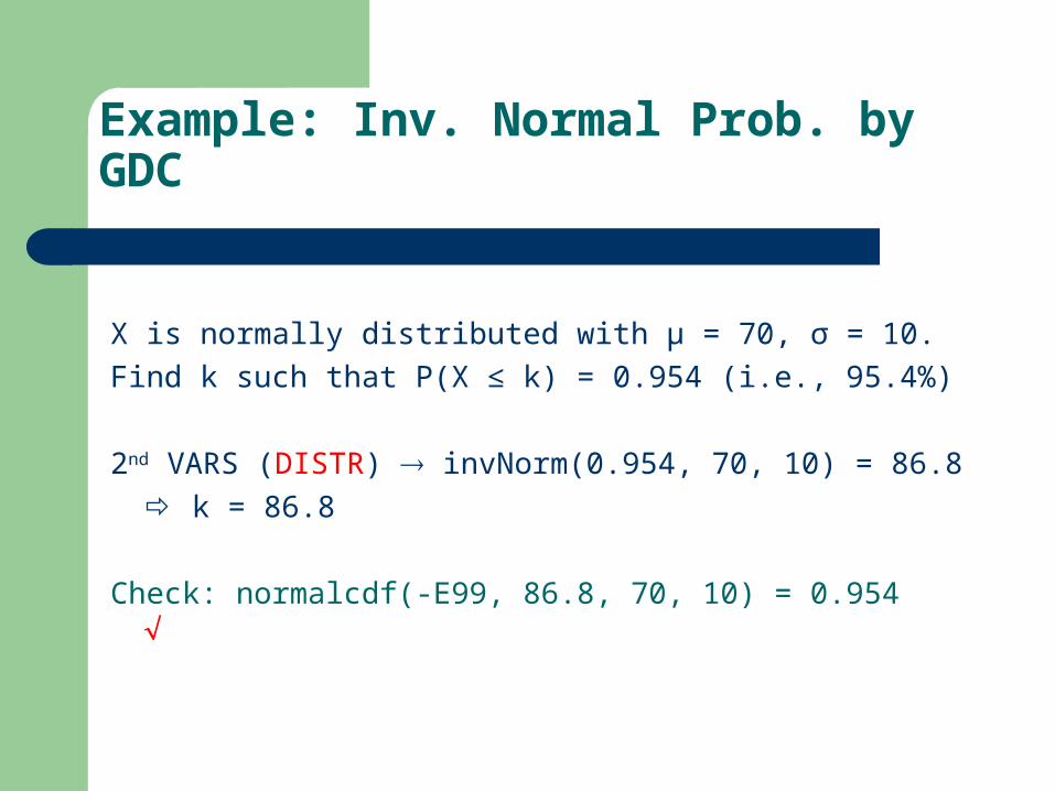
X is normally distributed with μ = 70, σ = 10.
Find k such that P(X ≤ k) = 0.954 (i.e., 95.4%)
2nd VARS (DISTR) invNorm(0.954, 70, 10) = 86.8
k = 86.8
Check: normalcdf(-E99, 86.8, 70, 10) = 0.954

Inverse Normal Probabilities by Table
Table in formula packet (2 pages)“Inverse Normal Probabilities (topic 6.11)”
Gives probability that Z is less than (actually < or ≤) a specified value
Table is for probabilities between 0.5 and 0.999, and only for positive values of Z
Before using table, convert X-values to Z
Reading Inverse Probability Table
(INSERT picture of table), with animations showing how to read z to 2 decimal places
Highlight probabilities on top and on left, highlight cross-indexed Z-score
Examples: Using Inverse Table
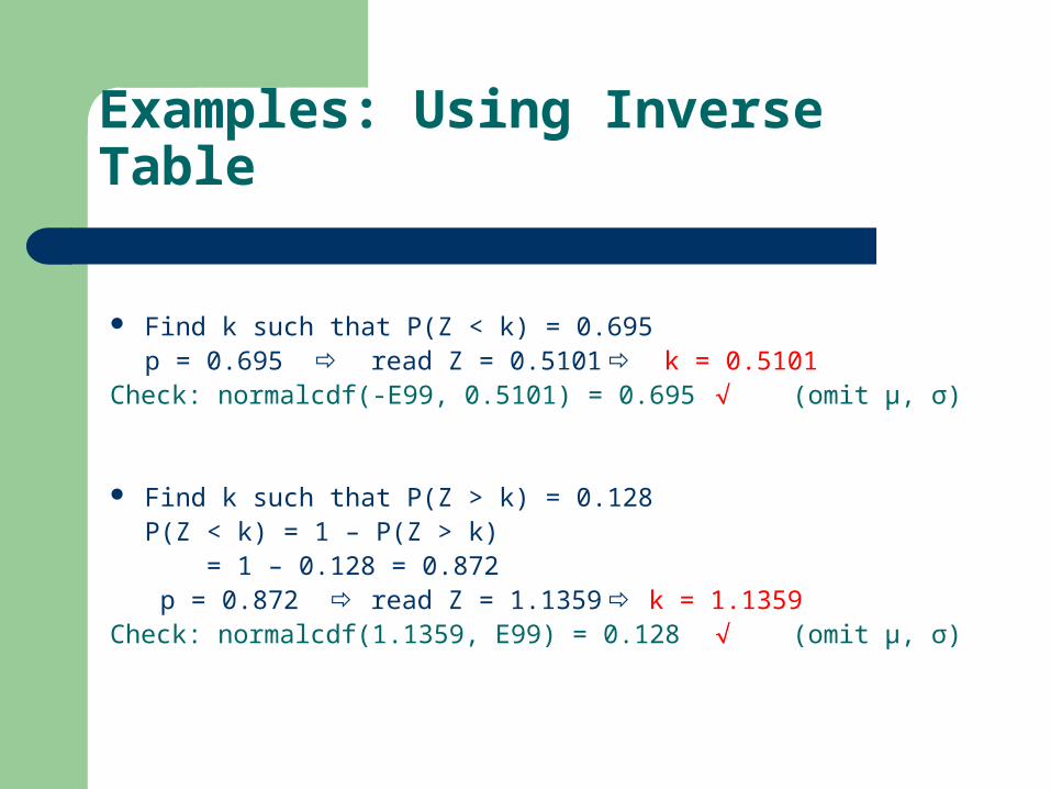
Find k such that P(Z < k) = 0.695p = 0.695 read Z = 0.5101 k = 0.5101
Check: normalcdf(-E99, 0.5101) = 0.695 (omit μ, σ)
Find k such that P(Z > k) = 0.128P(Z < k) = 1 – P(Z > k)
= 1 – 0.128 = 0.872 p = 0.872 read Z = 1.1359 k = 1.1359
Check: normalcdf(1.1359, E99) = 0.128 (omit μ, σ)

Example: Using Inverse Table for X
X is dist’d normally with μ = 24.6, σ = 0.8For what value of k is P(X < k) = 0.602?
p = 0.602 read Z = 0.2585 Z = (X – μ)/σ X = Zσ + μ
= (0.2585)(0.8) + 24.6 = 24.8
Check: normalcdf(-E99, 24.8, 24.6, 0.8) = 0.599 (difference due to rounding X)
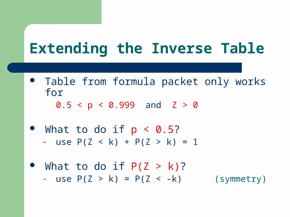
Extending the Inverse Table
Table from formula packet only works for0.5 < p < 0.999 and Z > 0
What to do if p < 0.5?– use P(Z < k) + P(Z > k) = 1
What to do if P(Z > k)?– use P(Z > k) = P(Z < -k) (symmetry)
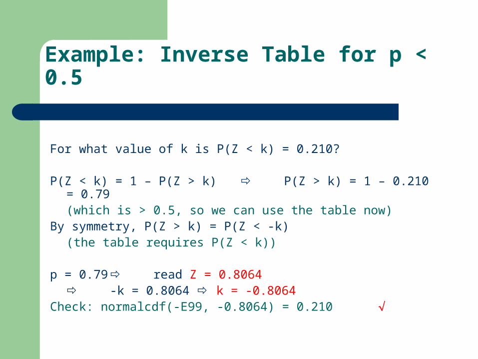
Example: Inverse Table for p < 0.5
For what value of k is P(Z < k) = 0.210?
P(Z < k) = 1 – P(Z > k) P(Z > k) = 1 – 0.210 = 0.79(which is > 0.5, so we can use the table now)
By symmetry, P(Z > k) = P(Z < -k)(the table requires P(Z < k))
p = 0.79 read Z = 0.8064 -k = 0.8064 k = -0.8064
Check: normalcdf(-E99, -0.8064) = 0.210
Example: Inverse Table, P(a < X < b)
Insert example…
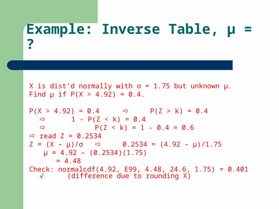
Example: Inverse Table, μ = ?
X is dist’d normally with σ = 1.75 but unknown μ.Find μ if P(X > 4.92) = 0.4.
P(X > 4.92) = 0.4 P(Z > k) = 0.4 1 - P(Z < k) = 0.4 P(Z < k) = 1 - 0.4 = 0.6
read Z = 0.2534Z = (X – μ)/σ 0.2534 = (4.92 – μ)/1.75
μ = 4.92 – (0.2534)(1.75) = 4.48
Check: normalcdf(4.92, E99, 4.48, 24.6, 1.75) = 0.401 (difference due to rounding X)