THE NRL MITE AIR VEHICLE

James Kellogg,1 Christopher Bovais,1 Jill Dahlburg,2 Richard Foch,1 John Gardner,3 Diana Gordon,4 Ralph Hartley4, Behrooz Kamgar-Parsi,4 Hugh McFarlane,1 Frank Pipitone,4 Ravi Ramamurti,3 Adam Sciambi,5 William Spears,4 Donald Srull,6 and Carol Sullivan1

ABSTRACT Micro Air Vehicles (MAVs) offer the promise of affordably expendable, covert sensor platforms for a range of close-in situational awareness activities. Since 1996, the US Naval Research Laboratory (NRL) has been developing technologies that will enable Navy-relevant missions with the smallest practical MAVs. This effort includes the development and integration of sensors, avionics, and advanced intelligent autopilots for flight control, with aerodynamic technologies. The NRL Micro Tactical Expendable (MITE) air vehicle is a result of this research. The operational MITE is a hand-launched, dual-propeller, fixed-wing air vehicle, with a 9-inch chord and a wingspan of 8 to 18 inches, depending on payload weight. The 14-inch MITE 2 can carry a one-ounce analog camera payload for mission flight durations in excess of 20 minutes, at air speeds of 10-20 miles/hour. While the MITE is presently a remote controlled air vehicle, both miniature �traditional� autopilots and also �advanced� autopilots, based on visual and spectral imaging techniques, are being developed. Autonomous MITEs will provide inexpensive, covert, highly portable sensor platforms for distribution and use in remote or urban environments. Multiple MITEs will provide distributed networks of roving and fixed sensor systems. 1Tactical Electronic Warfare Division, Naval Research Laboratory, Washington DC, USA 2General Atomics, San Diego CA, USA 3Laboratory for Computational Physics & Fluid Dynamics, Naval Research Laboratory, Washington DC, USA 4Artificial Intelligence Center, Naval Research Laboratory, Washington DC, USA 5Science & Engineering Apprentice Program, Naval Research Laboratory, Washington DC, USA 6CACI, Alexandria, Virginia, USA

Report Documentation Page Form ApprovedOMB No. 0704-0188

Public reporting burden for the collection of information is estimated to average 1 hour per response, including the time for reviewing instructions, searching existing data sources, gathering andmaintaining the data needed, and completing and reviewing the collection of information. Send comments regarding this burden estimate or any other aspect of this collection of information,including suggestions for reducing this burden, to Washington Headquarters Services, Directorate for Information Operations and Reports, 1215 Jefferson Davis Highway, Suite 1204, ArlingtonVA 22202-4302. Respondents should be aware that notwithstanding any other provision of law, no person shall be subject to a penalty for failing to comply with a collection of information if itdoes not display a currently valid OMB control number.

1. REPORT DATE 2001 2. REPORT TYPE

3. DATES COVERED 00-00-2001 to 00-00-2001

4. TITLE AND SUBTITLE The NRL Mite Air Vehicle

5a. CONTRACT NUMBER

5b. GRANT NUMBER

5c. PROGRAM ELEMENT NUMBER

6. AUTHOR(S) 5d. PROJECT NUMBER

5e. TASK NUMBER

5f. WORK UNIT NUMBER

7. PERFORMING ORGANIZATION NAME(S) AND ADDRESS(ES) Naval Research Laboratory,Artificial Intelligence Center,Washington,DC,20375

8. PERFORMING ORGANIZATIONREPORT NUMBER

9. SPONSORING/MONITORING AGENCY NAME(S) AND ADDRESS(ES) 10. SPONSOR/MONITOR’S ACRONYM(S)

11. SPONSOR/MONITOR’S REPORT NUMBER(S)

12. DISTRIBUTION/AVAILABILITY STATEMENT Approved for public release; distribution unlimited

13. SUPPLEMENTARY NOTES Proceedings of the Bristol RPV/AUV Systems Conference, Bristol, UK, April 2001

14. ABSTRACT Micro Air Vehicles (MAVs) offer the promise of affordably expendable, covert sensor platforms for arange of close-in situational awareness activities. Since 1996, the US Naval Research Laboratory (NRL) hasbeen developing technologies that will enable Navy-relevant missions with the smallest practical MAVs.This effort includes the development and integration of sensors, avionics, and advanced intelligentautopilots for flight control, with aerodynamic technologies. The NRL Micro Tactical Expendable (MITE)air vehicle is a result of this research. The operational MITE is a hand-launched, dual-propeller,fixed-wing air vehicle, with a 9-inch chord and a wingspan of 8 to 18 inches, depending on payload weight.The 14-inch MITE 2 can carry a one-ounce analog camera payload for mission flight durations in excess of20 minutes, at air speeds of 10-20 miles/hour. While the MITE is presently a remote controlled air vehicle,both miniature ’traditional’ autopilots and also ’advanced’ autopilots, based on visual and spectralimaging techniques, are being developed. Autonomous MITEs will provide inexpensive, covert, highlyportable sensor platforms for distribution and use in remote or urban environments. Multiple MITEs willprovide distributed networks of roving and fixed sensor systems.

15. SUBJECT TERMS

16. SECURITY CLASSIFICATION OF: 17. LIMITATION OF ABSTRACT Same as

Report (SAR)

18. NUMBEROF PAGES

13

19a. NAME OFRESPONSIBLE PERSON

a. REPORT unclassified

b. ABSTRACT unclassified

c. THIS PAGE unclassified

Standard Form 298 (Rev. 8-98) Prescribed by ANSI Std Z39-18

The Office of Naval Research has sponsored the Naval Research Laboratory (NRL) to conduct a Micro Air Vehicle (MAV) exploratory development research program. The goal of this MAV research is to develop and demonstrate MAV technology that supports Navy-specific applications and is complimentary and supplementary to the Defense Advanced Research Projects Administration (DARPA) MAV Program. Additional MAV requirements beyond the DARPA effort include Navy-specific applications, electric propulsion, non-Global Positioning System (GPS) navigation, and airframe size commensurate with operating conditions.

NRL developed a baseline design called the Micro Tactical Expendable (MITE) which consists of a low aspect ratio flying wing with dual, counter-rotating propellers mounted at the wing tips. This configuration was selected based on a tradeoff analysis that included aerodynamic performance, payload interface, launch and recovery methods, and compact storage. Specifically, the low wing aspect ratio is necessary to provide sufficient wing area within a compact wingspan. Although the low aspect ratio increases the induced drag of the wing, the increase in wing chord raises the Reynolds number, which improves the boundary layer characteristics, hence performance, of the airfoil. The dual propellers provide slipstream flow over nearly the entire wing for enhanced lift at low speeds. By counter rotating in the direction opposite of the wingtip vorticies, the Zimmerman Effect is produced, which reduces the induced drag to a value noticeably lower than expected for the low aspect ratio of the wing. Another benefit of counter-rotation is the balancing of torque and slipstream rotation effects, allowing high lateral stability at low speeds to enable easy hand launching of the MITE. As a flying wing, MITE uses elevon controls, which have enhanced effectiveness since they are also immersed in the slipstream. Payload location is in an unobstructed nose, which is ideal for imaging and accommodating a range of sensors. Despite being a flying wing with no geometric dihedral, the overall combination of design features results in a simple configuration possessing inherent stability about all three axes, good performance, ease of hand launch, and simple landing by gliding to the ground.

Wing Aspect Ratio vs. Reynolds Number for Minimum Drag

Fifty percent of the total drag for a well-

designed airplane, cruising at its best speed for range, is induced drag. When flying at best efficiency for endurance, the induced drag component is an even greater percentage of the total drag. The profile drag of the airfoil shape is a relatively small component of the overall airplane�s drag. Consequently, while airfoil designers strive to minimize profile drag, airplane designers must minimize induced drag to maximize range and endurance.

The induced drag of a wing is a result of a spanwise component of the airflow near the wingtips caused by the finite span of a wing. Induced drag is a function of the square of the lift coefficient and inversely proportional to the wing aspect ratio. Since the optimal cruise lift coefficient is a function of the airfoil, reducing induced drag requires increasing the aspect ratio, i.e. increasing the wing span-to-wing chord ratio. For a given wing loading, increasing the wing aspect ratio results in a reduction of the wing chord. Typically, the wing aspect ratio is as large as structural considerations allow, since reducing the chord reduces the wing thickness in proportion, while at the same time increasing the wing root bending moment since the wingspan is increased.

Fig. 1. Typical values of MAV wing chord Reynolds number.

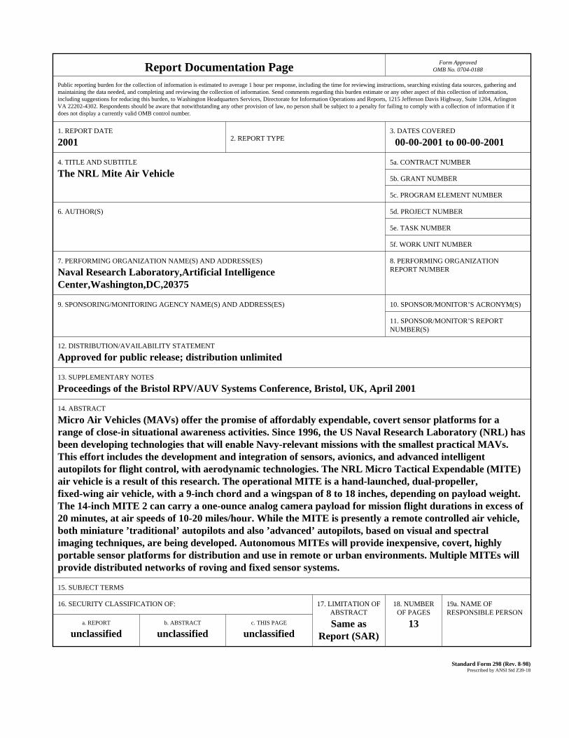
Unlike large aircraft, the maximum value of wing aspect ratio for an MAV is limited by airfoil aerodynamics before the structural limit is reached. The value of profile drag for a large aircraft is relatively constant with Reynolds number variations. However, in the aerodynamic regime of MAV airfoils, the profile drag coefficient increases in inverse proportion to the cube root of the Reynolds number. As the value of the airfoil�s profile drag begins to rise, a point is reached where it is no longer a minor drag component. As such, the design of an efficient MAV wing requires an optimization between minimizing induced drag without significantly increasing the airfoil profile drag. An empirical equation (Figure 2) was derived at NRL that can be used to determine an optimal tradeoff between induced drag and profile drag for MAVs. This equation substantiates why MAVs typically perform well with wings having lower aspect ratio than larger aircraft.

MAV Research Platforms

A number of exploratory miniature flight test vehicles have been designed and built to explore various vehicle design configurations, including a range of propulsion and control approaches. Design focused on minimum size air vehicles that were capable of performing potentially useful military missions. Maximum use was to be made of available, commercial items, while exploiting emerging, high pay-off technology where appropriate. The vehicles were also available to support the initial flight-testing of prototype and breadboard payload components and modules.

The test vehicles ranged in size from 8 inches to 18 inches, with gross weights of 1.5 to 12 ounces.

Early tests of miniature internal combustion, liquid fuel engine propulsion were abandoned in order to concentrate on electric motors employing high energy-density primary (single use) and secondary (rechargeable) cells. Electric propulsion, while not as weight/energy efficient as chemical fueled internal combustion engines, offered the potential for highly reliable, totally silent field operations plus extremely rapid

commercial technological growth. Early flight-testing of various motor configurations also indicated that twin motor layouts, compared to single motors, could provide simplified launching capability and possible control and aerodynamic advantages. Plank-type flying wing configurations proved to be compact, sturdy, and stable MITE platforms. Elevon plus synchronized or differential motor speed control provides adequate vehicle control. The principal MITE vehicles are described below.

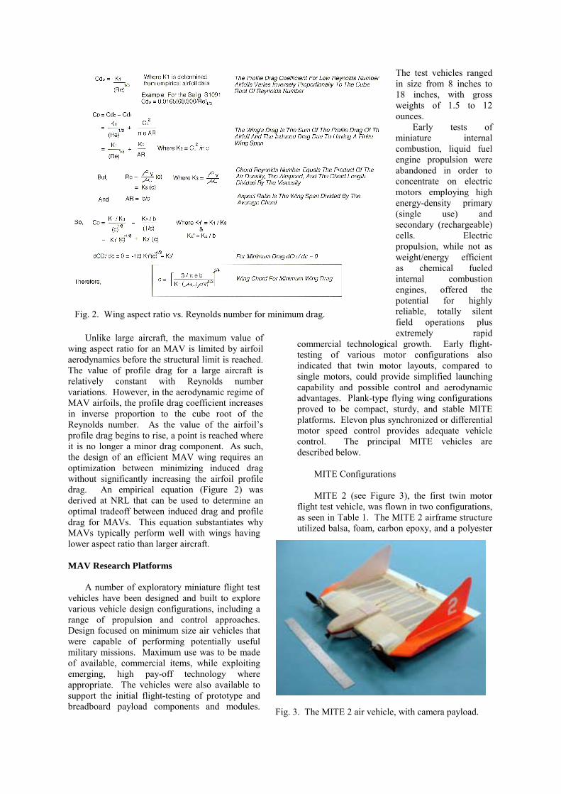
MITE Configurations MITE 2 (see Figure 3), the first twin motor

flight test vehicle, was flown in two configurations, as seen in Table 1. The MITE 2 airframe structure utilized balsa, foam, carbon epoxy, and a polyester

Fig. 2. Wing aspect ratio vs. Reynolds number for minimum drag.

Fig. 3. The MITE 2 air vehicle, with camera payload.

fiber covercells, it dabout 30 msmooth cam

A comon board vgleaned frvideo sysMITE 2 ve

MITEversion ofpowerful speed contversions alfor propulenergy andThese battmotor. Gounces.

MITEconfiguratidesigned tprototype to 4 ouncelarger wininches forpowerful (motors. Gto 9.0 oun

Span GrossMotoPropePropuCommPaylo

CommaControlMotor SMotorsProps BatteryCable HAirfram

Payload

Table 1 Configuration A Configuration B 14.5 inches 14.5 inches

Weight 4.5 ounces 7.5 ounces rs two 4 watt coreless, geared two 7 watt coreless, geared llers 7 inch dia., 8 inch pitch 7 inch dia., 8 inch pitch lsion Battery 9 volt LiSO2 primary (CR2) 12 volt Li SO2 primary (CR2) and Receiver single conv. FM 72Mhz dual conv. FM 72Mhz

ad none color video system

ing. In early tests using lithium primary emonstrated a maximum endurance of

inutes. It was a stable, and relatively era platform.

pack. Payloads of up to 3.5 ounces can be accommodated.

Motor/Battery System

The electric motors used in all MITE vehicles

to date are commercially available, coreless, permanent magnet motors. At relatively low output power levels of under 15 watts, coreless motors are lighter in weight and generally more efficient than conventional ferrite cored motors. Their electrical efficiency can be above 70%, although at power levels usually employed, 60% efficiencies are more common.

Because these motors are high RPM, low torque devices, gearing is used in all cases to turn efficient size propellers at lower speeds than the motor rotor. Gearing of up to 12:1 has been used, but current MITE vehicles typically use around 6:1 gear ratios to turn 7-inch diameter, 8-inch pitch propellers at speeds between 3,000 and 5,000 rpm. To achieve symmetrical propeller flow forces on

Table 2 MITE 2 Weight Breakdown

Item Weight, grams Ver. 2A Ver. 2B

nd Receiver 5 21 Servos 6 6 peed Control 5 6

25 25 7 7

Power Supply 34 45 arness, etc. 6 8 e Structure 41 41

sub-total 129 159 0 52

gross weight 129 211

petent pilot could fly the vehicle via the ideo system. Valuable experience was

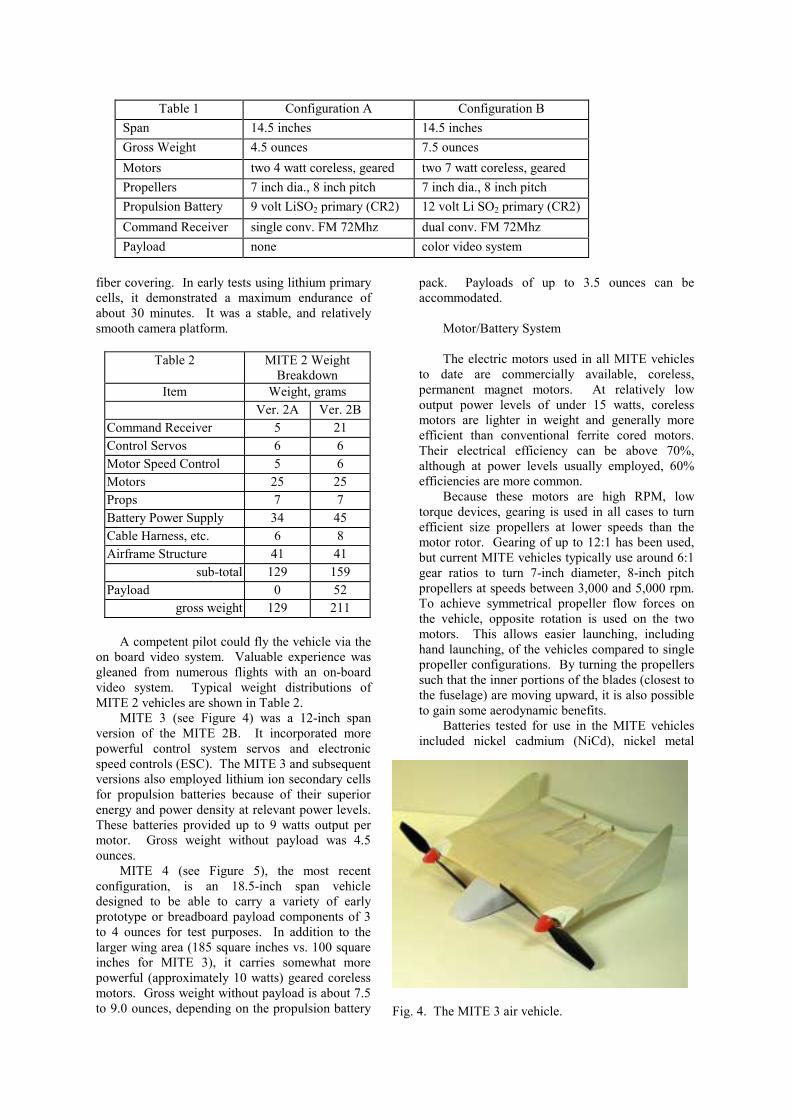
om numerous flights with an on-board tem. Typical weight distributions of hicles are shown in Table 2. 3 (see Figure 4) was a 12-inch span the MITE 2B. It incorporated more control system servos and electronic rols (ESC). The MITE 3 and subsequent so employed lithium ion secondary cells sion batteries because of their superior power density at relevant power levels. eries provided up to 9 watts output per ross weight without payload was 4.5

4 (see Figure 5), the most recent on, is an 18.5-inch span vehicle o be able to carry a variety of early or breadboard payload components of 3 s for test purposes. In addition to the

g area (185 square inches vs. 100 square MITE 3), it carries somewhat more approximately 10 watts) geared coreless ross weight without payload is about 7.5 ces, depending on the propulsion battery

the vehicle, opposite rotation is used on the two motors. This allows easier launching, including hand launching, of the vehicles compared to single propeller configurations. By turning the propellers such that the inner portions of the blades (closest to the fuselage) are moving upward, it is also possible to gain some aerodynamic benefits.

Batteries tested for use in the MITE vehicles included nickel cadmium (NiCd), nickel metal

Fig. 4. The MITE 3 air vehicle.

hydride (NiMH), and lithium ion secondary cells as well as lithium sulfur dioxide (LiSO2) primary cells. For discharge rates of 1 ampere or less, the lithium primary cells proved to be superior to all other cells tested. The nominal 3-volt, 750-mAh capacity CR2 cell, weighing less than 12 grams, was most efficient for use in the early lightweight MITE 2 test vehicles. For subsequent MITE vehicles, where higher power and current drains of 3 to 4 amperes was needed, lithium ion secondary cells of 430 and 800 mAh nominal capacity were used. As shown in Table 3, these cells provide much higher energy densities than comparable weight nickel cadmium or nickel metal hydride cells.

Table 3 Sample Cell Test Comparison Cell Weight,

gm Discharge

Rate, amps

Energy Capacity, watt min.

Energy Density,

watt min/gm

Av. Voltage

Delivered Capacity,

mAh

Cutoff Voltage

Cutoff Time, min.

430 mAh Tadiran 12.5 0.7 59.2 4.73 2.62 376 2.2 32.2 Lithium Rechargeable 1.0 44.9 3.59 2.53 294 2.2 17.7 1.5 32.0 2.56 2.47 216 2.2 8.6 2.0 18.3 1.47 2.36 130 2.2 3.9 800 mAh Tadiran 18.3 1.0 93.0 5.08 2.55 608 2.2 36.5 Lithium Rechargeable 1.5 82.6 4.50 2.56 538 2.2 21.5 2.0 71.7 3.92 2.51 476 2.2 14.3 2.5 60.2 3.29 2.39 420 2.2 10.1 3.0 46.7 2.55 2.40 324 2.2 6.5 750 mAh CR2 11.6 0.7 82.9 7.15 2.30 595 1.6 51.0 Lithium Primary 1.0 57.1 4.92 2.20 425 1.6 25.0 1.5 34.6 2.98 2.10 280 1.6 10.3 50 mAh Sanyo NiCd 3.6 0.5 4.7 1.31 1.14 35 0.8 4.1 1.0 1.8 0.50 0.99 31 0.8 1.8 1.5 1.1 0.29 0.99 27 0.8 1.1 80 mAh Sanyo NiCd 5.73 0.5 8.7 1.53 1.17 63 0.8 7.5 1.0 3.3 0.57 1.09 50 0.8 3.0 1.5 1.8 0.32 1.03 44 0.8 1.8 110 mAh Sanyo NiCd 7.3 0.5 6.7 0.91 1.19 94 0.8 11.3 0.7 6.7 0.91 1.16 90 0.8 7.8 1.0 6.1 0.82 1.12 90 0.8 5.4 1.5 5.5 0.74 1.07 86 0.8 3.5 2.0 5.2 0.70 1.00 82 0.8 2.5 120 mAh NiMH 3.5 0.7 7.1 2.00 1.01 105 0.8 9.1 1.0 5.7 1.60 0.95 92 0.8 5.6 1.5 4.9 1.40 0.94 84 0.8 3.4 270 mAh NiMH 7.5 1.5 17.0 2.30 1.03 278 0.8 11.1 2.0 15.0 2.00 0.95 255 0.8 7.7 2.5 13.0 1.70 0.93 234 0.8 5.6 3.0 10.0 1.30 88 135 0.8 3.7

Fig. 5. The MITE 4 air vehicle.

Computational Fluid Dynamics for MITE Vehicle Design

Computational fluid dynamics (CFD) plays an

important role in the design of low Reynolds number UAVs or MAVs. NRL has been using the FEFLO code, an unstructured finite element code based on tetrahedral elements, to investigate a range of small vehicles suitable for autonomous flight operation. CFD is used for two objectives. One is to determine optimal configurations from the aerodynamic performance point of view. The other is to determine the aerodynamic coefficients that serve as input to NRL�s six degrees of freedom flight simulator. This simulator is in turn used to evaluate stability, performance, and optimal control laws for the autopilot.

The CFD simulations are performed with the code FEFLO. This code was developed at NRL by Ravi Ramamurti and at The George Mason University, Fairfax, Virginia, by Rainald Löhner. The governing equations are the incompressible Navier-Stoles equations, which are solved in an Arbitrary Lagrangian Eulerian (ALE) formulation. The equations are discretized in time using an implicit time stepping procedure. It is important for the flow solver to be able to capture the unsteadiness in the flow field, if such exists. This is especially true in low Reynolds number vehicles where the separation bubble may be unsteady. The flow solver is time-accurate, allowing local timestepping as an option. The resulting expressions are subsequently discretized in space using a Galerkin procedure with linear tetrahedral elements. In order for the algorithm to be as fast as possible, the overhead in building element matrices, residual vectors, etc. must be kept to a minimum. This is accomplished by employing simple, low-order elements that have all the variables (three velocity components and pressure) at the same node location. The resulting matrix systems are solved iteratively using a

preconditioned conjugate gradient algorithm (PCG). The code has the options to be run Euler, laminar flow, or incorporate a Baldwin-Lomax turbulence model. The solver has been successfully evaluated for both two dimensional (2-D) and three dimensional (3-D), laminar and turbulent flow problems by Ramamuti et al. [1, 2].

Flow over small vehicles is significantly modified by the influence of the propeller. Time dependent simulation of the propeller would be very time consuming, and inconsistent with the desire to make many simulations of different configurations, at several vehicle attitudes, to determine the aerodynamic coefficients. Instead, it has been found to be adequate to model the propeller as an actuator disk with a distribution of axial and radial momentum sources that match the thrust and drag of the actual propeller.

Figure 6 shows the flow field over two different configurations. The first (Figure 6(a)) is the MITE vehicle with a wingspan of 6 inches and a span to wing cord aspect ratio of 1.25. The pressure contours on the body surface are shown. The dark regions indicate stagnation regions of high pressure. The high pressure in the stagnation regions around the wing body junction can be reduced by proper fairing. A number of configuration changes were looked at to find an optimal configuration. The inviscid calculations were performed with approximately 160K points and 860K tetraheda. For symmetric cases the simulations were performed over half of the vehicle assuming a symmetry plane at the axis. Figure 6(b) shows the MITE 2 configuration, a slightly larger vehicle with a wingspan of 14.5 inches and a cord of 10 inches. Also shown are the velocity contours for a simulation that included effects of the counter rotating propellers. The propeller rotation direction was chosen to counter the effect of the tip vortex and increase the effective aspect ratio. This simulation was at an angle of attack of 15 degrees. Note the induced

a. 6 inch span MITE b. MITE 2

Fig. 6. CFD simulations of the evolving NRL MITE air vehicles

separation at the wing body junction on the MITE realistic resolution and noise. The CFD

-0.60

-0.40

-0.20

0.00

0.20

0.40

0.60

0.80

1.00

-5.0 0.0 5.0 10.0 15.0 20.0

θ = 0°

θ = 5°

θ = 10°

θ = 15°

θ = -5°

θ = -10°

θ = -15°

θ = 0°, 5°

CL

αααα (deg.)

0.00

0.05

0.10

0.15

0.20

-5.0 0.0 5.0 10.0 15.0 20.0

θ = 0°θ = 5°θ = 10°θ = 15°θ = -5°θ = -10°θ = -15°θ = 0°, 5°

CD

αααα (deg.)

-0.40

-0.30

-0.20

-0.10

0.00

0.10

0.20

0.30

0.40

-5.0 0.0 5.0 10.0 15.0 20.0

θ = 0°θ = 5°θ = 10°θ = 15°θ = -5°θ = -10°θ = -15°θ = 0°, 5°

CM

z

αααα (deg.)

-0.05

0.00

0.05

-20.0 -15.0 -10.0 -5.0 0.0 5.0 10.0 15.0 20.0

α = 0°

α = 15°

CM

x

θθθθ (deg.)

Fig. 7. CFD derived aerodynamic coefficients for the MITE 2 configurations.

2 configuration at the high angle of attack. The results of the aerodynamic coefficients derived for the MITE 2 configurations are shown in Figure 7.

Autopilot Development

Autopilots provide a significant challenge for

small autonomous vehicles. While there are many UAV autopilots in production for operational systems, most commercial-off-the-shelf autopilots weigh 4-12 lb. This is much greater than the gross weight of the MITE class of vehicles. NRL has developed a number of autopilots in support of small UAVs. A recent example is the Lightweight Autopilot (LWAP), which, at 2 lb, meets the functional but not the physical requirements. In an attempt to reduce the weight of the autopilot we are pursuing a number of unconventional means of autopilot control. These are primarily aimed at reducing the number of sensors required to provide the necessary stability and directional control. To test these new algorithms, a six degree of freedom (6DOF) flight simulator was used, coupled to an autopilot routine that uses simulated sensors with

simulations are used to provide the aerodynamic coefficients and stability derivatives for the 6DOF code. Two types of algorithms are being pursued. One involves using data from optical sensors to provide attitude information or optical flow for collision avoidance. The other uses a more sophisticated processing of a more limited set of sensor input and relies on the inherent stability of the MITE 2 vehicle to achieve directional and altitude control. A control law has been found that will allow the MITE 2 vehicle to be flown autonomously with only altitude and heading information that can be provided by, for instance, a simple barometric pressure sensor and magnetic heading indicator. Additional sensors can be added that increase the functionality, albeit at the expense of additional weight.

Optical Flow Sensor Development for MAV Navigation

Optical flow sensing is a technique that allows a moving observer to sense the proximity of its surroundings and relative motion with a minimum

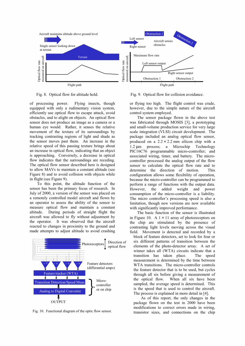
of processing power. Flying insects, though equipped with only a rudimentary vision system, efficiently use optical flow to escape attack, avoid obstacles, and to alight on objects. An optical flow sensor does not produce an image as a camera or a human eye would. Rather, it senses the relative movement of the texture of its surroundings by tracking contrasting regions of light and shade as the sensor moves past them. An increase in the relative speed of this passing texture brings about an increase in optical flow, indicating that an object is approaching. Conversely, a decrease in optical flow indicates that the surroundings are receding. The optical flow sensor described here is designed to allow MAVs to maintain a constant altitude (see Figure 8) and to avoid collision with objects while in flight (see Figure 9).

To this point, the altitude function of the sensor has been the primary focus of research. In July of 2000, a version of the sensor was placed on a remotely controlled model aircraft and flown by an operator to assess the ability of the sensor to measure optical flow and maintain a constant altitude. During periods of straight flight the aircraft was allowed to fly without adjustment by the operator. It was observed that the aircraft reacted to changes in proximity to the ground and made attempts to adjust altitude to avoid crashing

or flying too high. The flight control was crude, however, due to the simple nature of the aircraft control system employed.

The sensor package flown in the above test was fabricated through MOSIS [3], a prototyping and small-volume production service for very large scale integration (VLSI) circuit development. The package included an analog optical flow sensor, produced on a 2.2 × 2.2 mm silicon chip with a 1.2 µm process; a Microchip Technology PIC16C76 programmable micro-controller; and associated wiring, timer, and battery. The micro-controller processed the analog output of the flow sensor to calculate the optical flow rate and to determine the direction of motion. This configuration allows some flexibility of operation, because the micro-controller can be programmed to perform a range of functions with the output data. However, the added weight and power consumption of the micro-controller is a liability. The micro controller�s processing speed is also a limitation, though new versions are now available with significantly improved performance.

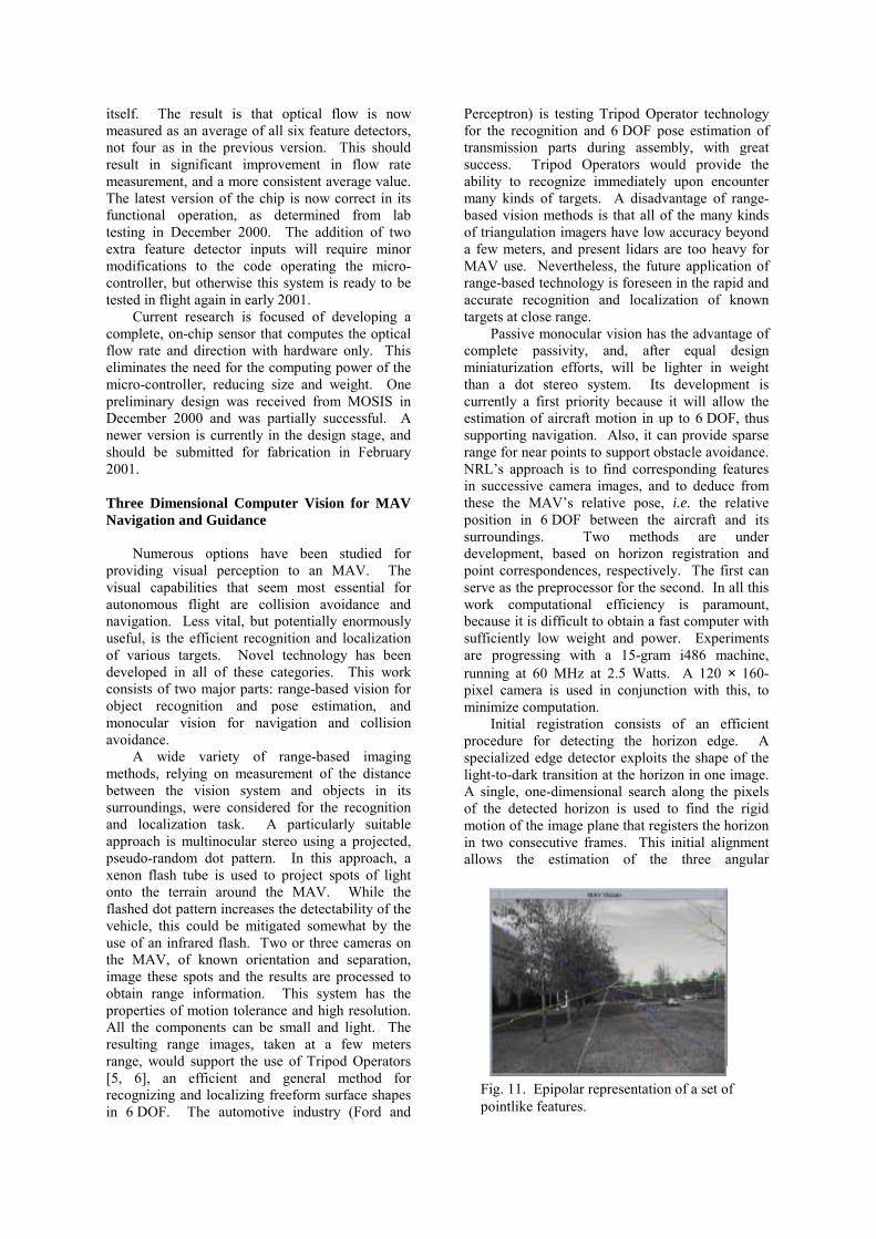
The basic function of the sensor is illustrated in Figure 10. A 1 × 11 array of photoreceptors on the chip are stimulated by the presence of contrasting light levels moving across the visual field. Movement is detected and recorded by a

block of feature detectors, set to look for four or six different patterns of transition between the elements of the photo-detector array. A set of winner takes all (WTA) circuits indicate that a transition has taken place. The speed measurement is determined by the time between WTA transitions. The micro-controller controls the feature detector that is to be used, but cycles through all six before giving a measurement of the optical flow. When all six have been sampled, the average speed is determined. This is the speed that is used to control the aircraft. The process is explained in more detail in [4].

As of this report, the only changes in the package flown on the test in 2000 have been modifications to correct errors made in wiring, transistor sizes, and connections on the chip

- + - + - + - +

Feature tracker (WTA)

Transition Detection/Speed Meas.

Analog to Digital Converter

OUTPUT

Direction ofoptical flow

Photoreceptors

Feature detectors(differential amps)

Micro-controlleror on chip

Fig. 10. Functional diagram of the optic flow sensor.

Terrain

Opt

ical

f low

rate

m

easu

r ed

on a

ircr a

ft

Flight path

Aircraft maintains altitude above ground level

Single sensor looking downat terrain

Opt

ical

flow

r ate

m

easu

r ed

on a

ircr a

ft

Flight path

Left sensor

Right sensor

Obstruction 2

Obstruction 1

Maximum flow rate

Left sensor output

Right sensor output

Obstruction 1 Obstruction 2

Aircraft sensesobstacles

Fig. 8. Optical flow for altitude hold. Fig. 9. Optical flow for collision avoidance.

itself. The result is that optical flow is now measured as an average of all six feature detectors, not four as in the previous version. This should result in significant improvement in flow rate measurement, and a more consistent average value. The latest version of the chip is now correct in its functional operation, as determined from lab testing in December 2000. The addition of two extra feature detector inputs will require minor modifications to the code operating the micro-controller, but otherwise this system is ready to be tested in flight again in early 2001.

Current research is focused of developing a complete, on-chip sensor that computes the optical flow rate and direction with hardware only. This eliminates the need for the computing power of the micro-controller, reducing size and weight. One preliminary design was received from MOSIS in December 2000 and was partially successful. A newer version is currently in the design stage, and should be submitted for fabrication in February 2001.

Three Dimensional Computer Vision for MAV Navigation and Guidance

Numerous options have been studied for

providing visual perception to an MAV. The visual capabilities that seem most essential for autonomous flight are collision avoidance and navigation. Less vital, but potentially enormously useful, is the efficient recognition and localization of various targets. Novel technology has been developed in all of these categories. This work consists of two major parts: range-based vision for object recognition and pose estimation, and monocular vision for navigation and collision avoidance.

A wide variety of range-based imaging methods, relying on measurement of the distance between the vision system and objects in its surroundings, were considered for the recognition and localization task. A particularly suitable approach is multinocular stereo using a projected, pseudo-random dot pattern. In this approach, a xenon flash tube is used to project spots of light onto the terrain around the MAV. While the flashed dot pattern increases the detectability of the vehicle, this could be mitigated somewhat by the use of an infrared flash. Two or three cameras on the MAV, of known orientation and separation, image these spots and the results are processed to obtain range information. This system has the properties of motion tolerance and high resolution. All the components can be small and light. The resulting range images, taken at a few meters range, would support the use of Tripod Operators [5, 6], an efficient and general method for recognizing and localizing freeform surface shapes in 6 DOF. The automotive industry (Ford and

Perceptron) is testing Tripod Operator technology for the recognition and 6 DOF pose estimation of transmission parts during assembly, with great success. Tripod Operators would provide the ability to recognize immediately upon encounter many kinds of targets. A disadvantage of range-based vision methods is that all of the many kinds of triangulation imagers have low accuracy beyond a few meters, and present lidars are too heavy for MAV use. Nevertheless, the future application of range-based technology is foreseen in the rapid and accurate recognition and localization of known targets at close range.

Passive monocular vision has the advantage of complete passivity, and, after equal design miniaturization efforts, will be lighter in weight than a dot stereo system. Its development is currently a first priority because it will allow the estimation of aircraft motion in up to 6 DOF, thus supporting navigation. Also, it can provide sparse range for near points to support obstacle avoidance. NRL�s approach is to find corresponding features in successive camera images, and to deduce from these the MAV�s relative pose, i.e. the relative position in 6 DOF between the aircraft and its surroundings. Two methods are under development, based on horizon registration and point correspondences, respectively. The first can serve as the preprocessor for the second. In all this work computational efficiency is paramount, because it is difficult to obtain a fast computer with sufficiently low weight and power. Experiments are progressing with a 15-gram i486 machine, running at 60 MHz at 2.5 Watts. A 120 × 160-pixel camera is used in conjunction with this, to minimize computation.

Initial registration consists of an efficient procedure for detecting the horizon edge. A specialized edge detector exploits the shape of the light-to-dark transition at the horizon in one image. A single, one-dimensional search along the pixels of the detected horizon is used to find the rigid motion of the image plane that registers the horizon in two consecutive frames. This initial alignment allows the estimation of the three angular

Fig. 11. Epipolar representation of a set of pointlike features.

coordinates of the aircraft�s frame-to-frame motion. In this application, frame-to-frame changes are very great, so that carefully designed matching procedures are necessary to find corresponding features in two frames.

After the change in the observed position of the horizon has provided an estimation of the MAV�s frame-to-frame change in attitude, the subsequent processes of estimating the MAV�s translational motion and of refining the three attitude angles is simplified. Using a carefully designed interest point detector, sparse pointlike features are detected in the two successive images. These could be the tips of tree branches or the corner of a building�features that can be easily and unambiguously localized as points. Not suitable are roof surfaces, road edges, tree limbs, and the like, or any object with a planar or linear appearance. With a small number of appropriately scattered points it is possible to compute the ranges of all the points, simultaneously with the change in pose of the aircraft, although one overall scale factor must be deduced, if it is desired, from presumed speed or from some known scene structure. The analysis is done in the context of epipolar geometry (see Figure 11). A description of this work is in Pipitone, et al [7]. The resulting pose estimates are then chained together to maintain a cumulative estimate of the aircraft�s motion. Given a known initial position and attitude at launch, the MAV is able to track its progress analogously to odometry with a ground robot, but in 6 DOF. The most useful of the pose parameters appears to be the azimuthal angle, since it provides the geographic bearing for navigation. Operating Swarms of MAVs

So far, this paper has not focused the problem

of operating a large number of vehicles in conjunction with each other. In this section, scenarios are considered in which one might need to control the behavior of swarms of vehicles, also called �agents.� A general framework is presented, which satisfies the objective of distributed control of a large number of agents that range in scale from neurons, nanobots, or micro-electromechanical systems (MEMS) to MAVs and satellites. It is assumed that an agent�s sensors perceive the world (including other agents), and an agent�s effectors make changes to that agent or the world (including other agents). Often, agents can only sense and affect nearby agents; thus the problem is usually one of �local� control. Sometimes control is also guided by global constraints and interactions.

One of the biggest problems is that is often unknown how to create the proper control rules for the operating scenarios. Agent behavior in these scenarios must satisfy challenging constraints. Not only does the desired global behavior of the agents

need to emerge from local agent interactions (i.e., self-assembly or self-organization), but there also needs to be some measure of fault-tolerance, i.e., the global behavior degrades very gradually if individual agents are damaged. Self-repair is also desirable, where a disrupted or damaged system repairs itself.

Self-assembly, fault-tolerance, and self-repair are precisely those principles exhibited by natural systems. Thus, many answers to the problems of distributed control may lie in the examination of the natural laws of physics.

This section proposes a general framework, called �physicomimetics,� for distributed control in which physics-inspired forces control agents. The term �physicomimetics� is used because the theory is motivated, but not restricted to, natural physical forces. Physicomimetics forces are not real forces; nevertheless the agents can act as if the forces are real. Thus the agent�s sensors must see enough to allow it to compute the virtual force to which it is reacting. The agent�s effectors must allow it to respond to this perceived force.

There are several potential advantages to this approach. First, in the real physical world, collections of small entities yield surprisingly complex behavior from very simple interactions. Thus there is a precedent for believing that complex control can be achieved through simple local interactions. This is required for very small agents (such as neurons or nanobots), since their sensors and effectors will necessarily be primitive. Also, since the approach is largely independent of the size and number of agents, the results should scale well to larger agents and larger sets of agents. Finally, such systems are potentially analyzable by physics analysis methods (e.g., statistical mechanics).

Physicomimetics Framework The motivation for this work stems from a

desire for swarms of MAVs to perform various tasks. This approach treats agents as physical particles, which could range in size from nanobots to satellites. A simple but realistic physical simulation of the particles� behavior was built. Particles exist in two (or three) dimensional worlds and are considered to be point-masses. Each particle p has position p = (x , y) and velocity v = (vx , vy). A discrete-time approximation to the continuous behavior of the particles is used, with time-step ∆t. At each time step, the position of each particle undergoes a perturbation ∆p. The perturbation depends on the current velocity ∆p = v ∆t. The velocity of each particle at each time step also changes by ∆v. The change in velocity is controlled by the force on the particle ∆v = F ∆t / m, where m is the mass of that particle and F is the

force on that particle. A frictional force is included, for self-stabilization.

For MAVs, the initial conditions are similar to those of a �big bang� � the MAVs are assumed to be released from a canister dropped from an airplane; they then spread outwards and perform their task. This is simulated by using a two-dimensional Gaussian random variable to initialize the positions of all particles (MAVs). Velocities of all particles are initialized to be 0, and masses are all 1 (although the framework does not require this). An example initial configuration for 100 particles is shown in Figure 12.

Given the initial conditions and some desired global behavior, the sensors, effectors, and force F laws need to be defined such that the desired behavior emerges. This is explored in the next few sections, for various tasks.

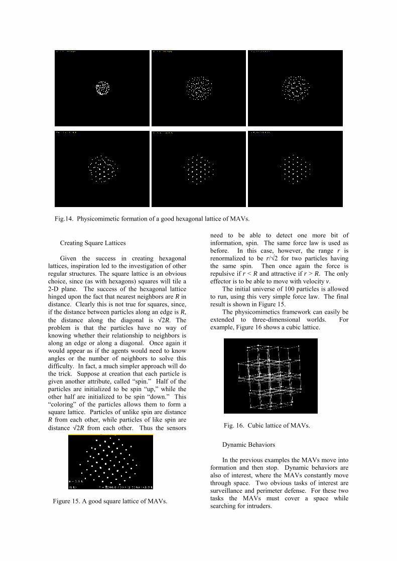
Creating Hexagonal Lattice Formations The example considered here is that of a

swarm of MAVs whose mission is to form a hexagonal lattice, which creates an effective sensing grid. Essentially, such a lattice will create a virtual antenna or synthetic aperture radar to improve the resolution of radar images. A virtual antenna is expected to be an important future application of MAVs. Currently, the technology for MAV swarms (and swarms of other micro-vehicles such as micro-satellites) is in the early research stage. Nevertheless we are developing the control software now so that we will be prepared.

Since MAVs have simple sensors and primitive CPUs, the goal was to provide the simplest possible control rules that require minimal sensors and effectors. At first blush, creating hexagons would appear to be somewhat complicated, requiring sensors that can calculate range, the number of neighbors, their angles, etc. However, it turns out that only range information is required. To understand this, recall an old high-school geometry lesson in which six circles of radius R can be drawn on the perimeter of a central circle of radius R (the fact that this can be done with only a compass and straight-edge can be proven with Galois theory). Figure 13 illustrates this construction. If the particles (shown as small circular spots) are deposited at the intersections of the circles, they form a hexagon.

To map this into a force law, imagine that each particle repels other particles that are closer than R, while attracting particles that are further than R in distance. Thus each particle can be considered to have a circular �potential well� around itself at radius R − neighboring particles will want to be at distance R from each other. The intersection of these potential wells is a form of constructive interference that creates �nodes� of very low

potential energy where the particles will be likely to reside (again these are the small circular spots in the previous figure). Thus the particles serve to create the very potential energy surface to which they respond. The entire potential energy surface is never actually computed. Particles only compute local force vectors for their current locations.

With this in mind a force law is defined F = G mi mj / r2

where F is the magnitude of the force between two particles i and j, and r is the range between the two particles. The �gravitational constant� G is set at initialization. The force is repulsive if r < R and attractive if r > R. Each particle has one sensor that can detect the range to nearby particles. The only effector is to be able to move with velocity v. To ensure that the force laws are as local as possible in nature, particles have a visual range of only 1.5R.

The initial universe of 100 particles (as shown in Figure 12) is now allowed to run, using this very simple force law. For a radius R of 50 we have found that a gravitational constant of G = 1200 provides good results, as can be seen in Figure 14.

The hexagonal lattice is not perfect � the final perimeter is not a hexagon, although this is not surprising, given the lack of global constraints. However, many hexagons are clearly embedded in the structure and the overall structure is quite hexagonal. It is also interesting to note that each node in the structure can have multiple particles (i.e., multiple particles can �cluster� together). Clustering was an emergent property that was not expected, and it provides increased robust behavior, because the disappearance (failure) of individual particles (agents) from a cluster will have minimal effect. This form of fault-tolerance is a result of the setting of G.

Fig. 12. The initial MAV universe at t = 0.

Figure 13. How circles can create hexagons.

Creating Square Lattices Given the success in creating hexagonal

lattices, inspiration led to the investigation of other regular structures. The square lattice is an obvious choice, since (as with hexagons) squares will tile a 2-D plane. The success of the hexagonal lattice hinged upon the fact that nearest neighbors are R in distance. Clearly this is not true for squares, since, if the distance between particles along an edge is R, the distance along the diagonal is √2R. The problem is that the particles have no way of knowing whether their relationship to neighbors is along an edge or along a diagonal. Once again it would appear as if the agents would need to know angles or the number of neighbors to solve this difficulty. In fact, a much simpler approach will do the trick. Suppose at creation that each particle is given another attribute, called �spin.� Half of the particles are initialized to be spin �up,� while the other half are initialized to be spin �down.� This �coloring� of the particles allows them to form a square lattice. Particles of unlike spin are distance R from each other, while particles of like spin are distance √2R from each other. Thus the sensors

need to be able to detect one more bit of information, spin. The same force law is used as before. In this case, however, the range r is renormalized to be r/√2 for two particles having the same spin. Then once again the force is repulsive if r < R and attractive if r > R. The only effector is to be able to move with velocity v.

The initial universe of 100 particles is allowed to run, using this very simple force law. The final result is shown in Figure 15.

The physicomimetics framework can easily be extended to three-dimensional worlds. For example, Figure 16 shows a cubic lattice.

Dynamic Behaviors In the previous examples the MAVs move into

formation and then stop. Dynamic behaviors are also of interest, where the MAVs constantly move through space. Two obvious tasks of interest are surveillance and perimeter defense. For these two tasks the MAVs must cover a space while searching for intruders.

Fig.14. Physicomimetic formation of a good hexagonal lattice of MAVs.

Figure 15. A good square lattice of MAVs.

Fig. 16. Cubic lattice of MAVs.

To achieve this the above framework is used, but with inter-agent attraction turned off. The agents repel each other, but are attracted to intruders that they can detect. They also require a means of sensing the limits of their operating area. The net effect is similar to a simulation of gas molecules in a container. Figures 17 and 18 show examples of MAVs performing surveillance and

perimeter defense. In both figures, an intruder is depicted by a small square. Note how some of the agents cluster in the square, thus �attacking� the intruder. These snapshots are static, and it is important to remember that the agents are in fact continually moving.

A nice aspect of this framework is its robustness. If agents are lost, the �gas� becomes more diffuse, but the agents still perform the task, although somewhat less efficiently. Moreover, the addition of new agents is also handled gracefully.

Future work will focus on other behaviors and formations. As applications arise, they will suggest new operating scenarios for which physicomimetics solutions will be derived.

References [1] RAMAMURTI, R and LÖHNER, R.,

Evaluation of an Incompressible Flow Solver Based on Simple Elements, Advances in Finite Element Analysis in Fluid Dynamics, 1992, FED Vol. 137, Editors: M.N. Dhaubhadel et al., ASME Publication, New York, pp. 33-42.

[2] RAMAMURTI, R., LÖHNER, R., and SANDBERG, W.C., Evaluation of Scalable 3-D Incompressible Finite Element Solver, AIAA paper No. 94-0756, 1994.

[3] MOSIS, Information Sciences Institute, University of Southern California, 4676 Admiralty Way, Marina del Rey CA, USA, 90292-6695, www.mosis.edu.

[4] MILLER and BARROWS, G., Feature Tracking Linear Optic Flow Sensor Chip, IEEE International Symposium on Circuits and Systems, 1999.

[5] PIPITONE, F., Tripod Operators for Realtime Recognition of Surface Shapes in Range Images, Proc. NASA Technology 2004 Symposium, Washington DC, November 1994.

[6] PIPITONE, F., A Method for Estimating the Pose of Surface Shapes in Six Degrees of Freedom from Range Images Using Tripod Operators, US Patent Pending, Navy Case Number 79822.

[7] PIPITONE, F., KAMGAR-PARSI, B., and HARTLEY, R., Three Dimensional Computer Vision for Micro Air Vehicles, Proc. SPIE 15th Aerosense Symposium, Conf. 4363, Enhanced and Synthetic Vision 2001, April 2001, Orlando FL.

Figure 17. MAVs performing area surveillance.

Figure 18. MAVs performing perimeter defense.