The Numerical Solution of Obstacle Problem by … Numerical Solution of Obstacle Problem by Self Adaptive Finite Element Method LIAN XUE, MINGHUI WU* Schood of Computer and Computing

The Numerical Solution of Obstacle Problem by Self Adaptive Finite

Element Method

LIAN XUE, MINGHUI WU*

Schood of Computer and Computing Science

Zhejiang University City College

Huzhou Street 51, Hangzhou 310015

P.R. CHINA

*corresponding author email: [email protected]

Abstract: - In this paper, the bisection of the local mesh refinement in self adaptive finite element is applied

to the obstacle problem of elliptic variational inequalities .We try to find the approximated region of the

contact in the obstacle problem efficiently .Numerical examples are given for the obstacle problem.

Key-Words: - obstacle problem, variational inequalities, self adaptive finite element, bisection, triangulation

refinement

1 Introduction The history of the study about self adaptive mesh is

more than 30 years, domestic and foreign

researchers have proposed various algorithms. The

self adaptive finite element method is a process

which estimates calculation error according to the

results of finite element method based on the

existing grid and then re-partition the grid where the

error is large and re-calculated. When the error is up

to the required value, the self adaptive process stops.

Therefore, effective error estimation and self

adaptive mesh generation are the two key

technologies of self adaptive finite element method.

The obstacle problem is one of the simplest

unilateral problems, it arises when modelling a

constrained membrane in the classical elasticity

theory. Many important problems, such as the

torsion of an elastic-plastic cylinder, the Stefan

problem can be formulated by transformation to an

obstacle problem. Several comprehensive

monographs can be consulted for the theory and

numerical solution of variational inequalities,

e.g.[1]-[4].Since obstacle problems are highly

nonlinear, it is difficult for the computation of

approximate solutions. The approximate solution of

obstacle problems is usually solved by variable

projection method, for example, the relaxation

method [2], multilevel projection method[5],

multigrid method[6]-[7] and projection method[8]

for nonlinear complementarity problems.

In most finite element methods that can be

applied to the obstacle problem, the error estimates

are acquired under regular and quasi-conforming

subdivision [9], but research on anisotropic

subdivision is less, which limits the application of

the finite element method in engineering. This paper

mainly discusses the numerical solution to elliptic

partial differential equations and the bisection

method is applied to the self adaptive finite element

method which will be applied to the obstacle

problem. The following is the variational principle

of elliptic boundary value problems. First of all,

consider the boundary value problem

*

,

0,

u f in

u on

= Ω

= ∂Ω

L

B (1)

WSEAS TRANSACTIONS on MATHEMATICS Lian Xue, Minghui Wu

ISSN: 1109-2769 285 Issue 5, Volume 9, May 2010

In this equation, Ω is the bounded

domain of dR , the border is Γ = ∂Ω , *∂Ω

can be the part of the border of ∂Ω or the

entire border. L is the linear differential

operators, B is the boundary operator.

The problem (1) is about how to find the

solution u in the sets of function that make (1)

meaningful. In this paper ,L is the uniform

operator of 2m orders, that is:

( ) ( )( )

( ) ( )( ) ( )

1 , ,

1 , principal part

d

m m

m

m

a x R

a x

β β ααβ

α β

β ααβ

α β

α β +≤ ≤

= =

= − ∂ ∂ ∈

= − ∂ ∂

∑ ∑

∑

0

L

L

(2)

And there is constant 0 0α > such that:

( )

( )

2 1

0 , ,

. . , ,

m d

m

d

a x m R R

a e x R a

α βαβ

α β

αβ

ξ α ξ α

ξ

++ +

= =

∞

≥ ∀ ∈ ∈

∀ ∈Ω ∈ ∈ Ω

∑

L

B is the homogeneous Dirichlet boundary

operator, that is on the ∂Ω ,

2 1

0, 0, 0, , 0

mu

u u uν ν ν

−∂ ∂ ∂ = = = = ∂ ∂ ∂

⋯

(3)

Here ( )1, , dν ν ν= ⋯ is the unit outer normal

vector on∂Ω . As long as ∂Ω is full-smooth,

(3) is meaningful. Especially when 1m = , (3) is

0u = . By the Sobolev space theory it’s easy to

know that conditions (3) can guarantee

( )0

mu∈ ΩH .

If ( ) ( )2

0

m mu∈ Ω ∩ ΩC H is the solution

of boundary value problem defined by (2) and

(3), in order to derive the variational form and

bilinear form, for any ( )0v ∞∈ ΩC , there is

( ) ( ) ( ) ( )0

,

, , 1a u v u v v a x udxβ β α

αβα β

Ω= = − ∂ ∂∑ ∫L

Here ( )0

,u vL is the inner product of ( )2 ΩL .

By the Green formula: for any 1, ( )u v∈ ΩC

, 1,2, ,i

i i

u vvdx u dx uv ds i d

x xν

Ω Ω ∂Ω

∂ ∂= − + =

∂ ∂∫ ∫ ∫ ⋯

(4)

We could get the variational form of elliptic

boundary value problems (2):

( ) ( ) ( )( ) ( )( )

( ) ( ) ( ) ( ) ( ),

00

,

,

m

a u v a x u x v x dx

f x v x dx f v F v v

α βαβ

α βΩ

≤

∞

Ω

= ∂ ∂

= = = ∀ ∈ Ω

∑ ∫

∫ C

Conversely, if ( )2mu∈ ΩC is the solution of

problem (4) whose boundary condition is (3). By

the Green formula (4), we can get

( ) ( )00,f u vdx v ∞

Ω− = ∀ ∈ Ω∫ L C

That is u f=L . In other words, the solution of

variational problem that meet the boundary

conditions (3) is the same as the original

boundary value problem’s. Therefore, for the

purposes of classical solutions, boundary value

problem and variational problem is equivalent,

but classical solution u of the boundary

conditions (3) satisfies ( ) ( )2

0

m mu∈ Ω ∩ ΩC H .

By the above-mentions the original

solution ( )0

mu∈ ΩH , also by the condition that

( )0

m ΩH is the closure of ( )2m ΩC under the

norm of ( )m ΩH . Therefore, the boundary

problem’s variational form or week form can be

written to: Finding ( )0

mu∈ ΩH such that

( ) ( )0

, ,a u v f v= ( )0

mv∀ ∈ ΩH (5)

The solution u of (5) is in ( )0

m ΩH and there



is not necessarily ( )2mu∈ ΩC , therefore, the

solution of (5) is the weak solution for the

boundary value problem (1).

The obstacle problem is a typical example of the

elliptic variational inequality of the first kind.

Consider the obstacle problem : Findu K∈ such

that

( ) inf ( )v K

E u E v∈

= (6)

Where

1

0K = H ( ) | . . v v a e inψ∈ Ω ≥ Ω (7)

21( ) ( | | )

2E v v fv dx

Ω= ∇ −∫ (8)

And the obstacle functionψ satisfies the condition 1( ) ( )H Cψ ∈ Ω Ω∩ and 0ψ ≤ onΓ , the boundary

of the domain Ω . Problems (6)-(8) describe the

equilibrium position u of an elastic membrane

constrained to lie above a given obstacleψ under an

external force 2( ) ( )f x L∈ Ω . It is well known that

the solution of (6)-(8) is characterized by the

following variational inequality: find u K∈ , such

that

( ) ( ) ,u v u dx f v u dx v KΩ Ω

∇ ⋅ ∇ − ≥ − ∀ ∈∫ ∫ (9)

If the solution 2 1

0( ) ( )u C H∈ Ω Ω∩ , then we have

1 2Ω = Ω Ω∪ －the coincidence set 1Ω and its

complement 2Ω ,

1, 0,u and u f inψ= − ∆ − > Ω (10)

2, 0,u and u f inψ> − ∆ − = Ω (11)

Notice that the region of contact

1 | ( ) ( )x u x xψΩ = ∈Ω = (12)

is an unknown a priori.

In this paper, we will apply the newest

bisection of the local mesh refinement in self

adaptive finite element method to solve the obstacle

problem (6)-(8). We first present the obstacle

problem and its numerical approximation by finite

element method. In section 2, we apply the self

adaptive finite element method to the obstacle

problem. In section 3, the self adaptive finite

element method is applied to one example of the

obstacle-free problem and the obstacle problem,

the implementation is achieved in MATLAB.

2 The Numerical Algorithm The finite element method is one of the most

commonly used discretization methods for the

numerical simulation of many practical models.

Now we apply the fininte element method to the

obstacle problem. We present the discreted obstacle

problem by the finite element method. Let

1

0 ( )hV H⊂ Ω be a linear finite element space. The

discrete adimissible set is

| ( ) ( ), h h h hK v V v x x for any node xψ= ∈ ≥ (13)

Then the approximation of problem (1)-(3) is to find

h hu K∈ such that

( ) inf ( )h h

h hv K

E u E v∈

= (14)

The error estimate in 1H norm or L∞

norm was

proved in [2,10,11].

Theorem 2.1 Assume that the solution u of (6)-( 8)

and the obstacle function ψ are in the space

2,W ∞ . Then, there exists a constant C

independent of h and solution hu of (8) satisfies

2

0, 2, 2,| log( ) | ( )hu u Ch h u ψ

∞ ∞ ∞− ≤ + (15)

To speed up computing numerical simulations,

AFEM (adaptive finite element method) is

introduced to reduce computational costs while

keeping optimal accuracy.

Now we discuss the self adaptive finite

element method and algorithm of this article. When

we do the mechanical analysis of engineering



structures, we did not know the extent of stress

concentration and its location. Mesh is refined in

the areas of large stress gradient only by virtue of

experience. But self adaptive finite element method

re-partition the grid through the error analysis of

finite element method so as to use the least degree

of freedom to obtain the best results in the range of

error allowed and avoid mesh density is too small

where stress gradient is large, or small stress

gradient is over the local mesh density. Here we

only discuss the tag strategy of triangulation in the

realization of the process.

2.1 Application of Bisection Method in the

self adaptive finite element method

We first introduced the two important properties of

triangulation.The triangulation hT of 2RΩ ⊂ (or

in grid) is the sets which divided Ω into a series

of triangles. Family Triangulation is conforming, if

the intersection of two triangles τ and 'τ in hT

is made up by the common vertex ix or edges E

or empty set (not intersect). Edge of a triangle is

called non-conforming, if there is a vertex, and it

falls on this edge, this vertex is called within the

next hanging point. To the suspension grid points, it

may need some specific base vector and matrix

assemblied complexly. For a conforming grid only

needs a set of base vectors of finite element. In the

following, we will have been used this property of

triangulation.

If ( )2diam

maxhτ

τσ

τ∈≤

T

that ( )diam τ is the

diameter of τ ， τ is the area of τ , we say family

triangulation is regular. If σ is independent of k

in the formula above, family triangulation is

uniformly regular. Regular triangulation ensure that

each corner of the triangular element are maintained

to0 π− . It’s important to the 1H norm estimates

of controlled error and the condition number of

stiffness matrix. After the marked triangle set is

refined, it needs to design a criterion for the

triangular element partitioned and marked so that

the refined grid remains the conformity and

regularity. Nowadays the most popular two methods

are as follow:

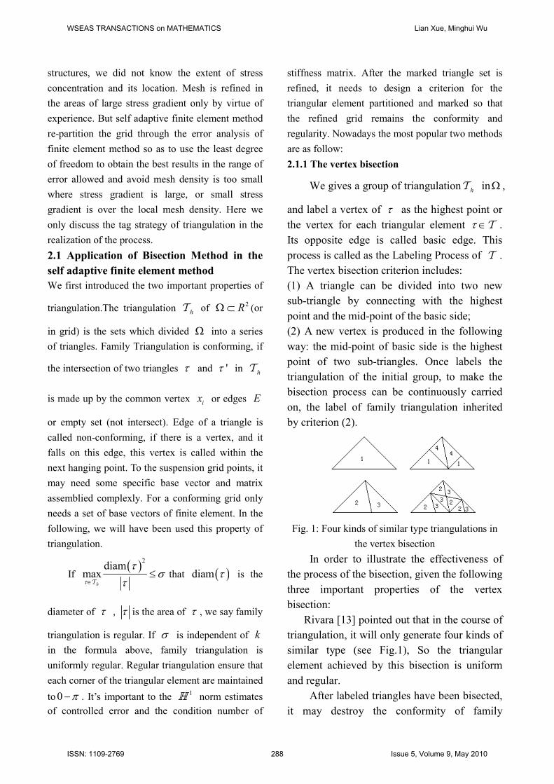
2.1.1 The vertex bisection

We gives a group of triangulation hT inΩ ,

and label a vertex of τ as the highest point or the vertex for each triangular element τ ∈T .

Its opposite edge is called basic edge. This

process is called as the Labeling Process of T .

The vertex bisection criterion includes:

(1) A triangle can be divided into two new

sub-triangle by connecting with the highest

point and the mid-point of the basic side;

(2) A new vertex is produced in the following

way: the mid-point of basic side is the highest

point of two sub-triangles. Once labels the

triangulation of the initial group, to make the

bisection process can be continuously carried

on, the label of family triangulation inherited

by criterion (2).

Fig. 1: Four kinds of similar type triangulations in

the vertex bisection

In order to illustrate the effectiveness of

the process of the bisection, given the following

three important properties of the vertex

bisection:

Rivara [13] pointed out that in the course of

triangulation, it will only generate four kinds of

similar type (see Fig.1), So the triangular

element achieved by this bisection is uniform

and regular.

After labeled triangles have been bisected,

it may destroy the conformity of family



triangulation. In order to restore conformity, in

the bisection process we should eliminate

hanging points, this process can be described as

perfection. The perfection process may generate

more hanging points, so it needs to stop the

process. This issue will be discussed in the

following. The last property for the AFEM

optimization problem is very important. It

points out that compared to the marked units,

the perfection process will not increase many

units.

2.1.2 The longest edge bisection

The longest edge bisection is proposed by

Rivara’s study group [16,17]. In this method,

the longest edge of the triangle is always used

for second-class subdivision. Every time the

maximum angle is divided in the longest edge

bisection. Therefore, we can expect that this

bisection can remain regularity.

In fact, Rosenberg and Stenger [20]

proved that in the process of dividing the

triangle the smallest angle is at least half of the

smallest angle of the initial triangle. Rivara

pointed out that this perfection process must be

terminated. It can be seen that the longest edge

bisection is a special case of the latest top

bisection in which different labels are used.

2.1.3 Labeling process to reduce error

We suppose 2 2

ττ

η η∈Τ

= ∑ is the cumulative

error index of local error contribution τη in a

triangular element τ . For the traditional labeling

strategy, it marks family triangulation so that:

( )* max , 0,1h

ττ τη θ η θ

∈Τ≥ ∀ ∈

This labeling strategy was first proposed by

Babuska and Vogelius [4].

Here we used the volume- marked strategy

raised by Dorfler. This strategy defines a tag

setM .so that

( )2 2 , 0,1M

ττ

η θη θ∈

≥ ∀ ∈∑

The larger θ makes more triangles to be

refined in a circle. Although the smaller θ can

lead to grid optimization in the result, it can lead to

more refined cycle. Generally, we choose

0.2 0.5θ = − .The advantage of the volume-

marked strategy is: For some elliptic problems, it

can prove that the approximation error of the fixed

factor for each cycle is diminishing. Therefore, this

partial refinement process is convergent. For many

degrees of freedom, its best numerical

approximation has been put forward.

2.1.4 Perfection

After the triangle has been marked by the

bisection, the major problem become: How to

maintain the conformity of the grid? We first

consider the process of the two basic approaches in

perfection, followed by a new strategy for edge

marking.

A standard iterative algorithm of perfection is

given as follows. Suggest, M is the triangle set

which need refinement. Mitchell proposed a more

efficient iterative algorithm, Kossaczky extend it to

3-D.

This approximation algorithm is based on the

following steps: If a triangle is non-conforming,

while we apply a single partition to the triangle

opposite to its highest point, it will become

conforming. Of course, its adjacent triangles may

also be non-conforming. Therefore, in this

algorithm it is repeatedly asked to check the

adjacent triangle, until we find a conforming

triangle. Because it always appears in the iteration

before the bisection, there always apper a pair of

conforming triangle when the second division is

occured(Except near its borders), and also to ensure

conformity. Mitchell proved that if the initial

triangulation is the label of conformity, this iteration

would be terminated.

2.1.5 marking the edge to Ensure conformity

In order to achieve conformity, we will put

forward the new approximation method in this part .

Noted that in the output of the grid, new nodes are

always those mid-points of some edges in the



inputed grid. Our labeling strategy is: If one side is

marked, basic sides of all the triangles sharing this

side will be marked.

It is only need slightly modified triangulation

( )τ , we will be able to achieve this tag by iteration.

Because in each iteration an edge must be marked,

and the number of edges of the triangulation is

limited, so the termination of this iterative algorithm

is obvious.

2.2 The numerical solution of obstacle

problem by the self adaptive finite element

method

AFEMs are now widely used in the numerical

solution of PDEs to achieve better accuracy with

minimum degrees of freedom. A typical loop of

AFEM through local refinement involves

solution error estimation

labeling triangular element refinement

→ →

→

More precisely to get a refined triangulation from

the current triangulation, we first solve the PDE to

get the solution on the current triangulation. The

error is estimated using the solution, and used to

mark a set of triangles that are to be refined.

Triangles are refined in such away to keep two most

important properties of the triangulations: shape

regularity and conformity.

Recently, several convergence and optimality

results have been obtained for adaptive finite

element methods on elliptic PDEs [12]-[17] which

justify the advantage of local refinement over

uniform refinement of the triangulations. In most of

those works, newest vertex bisection is used in the

refine step. It has been shown that the mesh

obtained by this dividing rule is conforming and

uniformly shape regular. In addition the number of

elements added in each step is under control which

is crucial for the optimality of the local refinement.

Therefore we mainly discuss vertex bisection in this

report and include another popular bisection rule,

longest edge bisection, as a variant of it.

From the paper [19,20], we can see that the

mesh is refined in the areas of large error by self

adaptive finite element method. The self adaptive

finite element method re-partition the grid through

the error analysis of finite element method so as to

use the least degree of freedom to obtain the best

results in the range of error allowed and avoid mesh

density is too small where stress gradient is large, or

small stress gradient is over the local mesh density.

In the paper [19,20], the author proposed bisection

method in the self adaptive finite element method

and prove its convergence. In the following, we will

apply this method to the discreted obstacle method,

which can be obtained by the numerical algorithm

in the paper [21] or [22].

Suggest 1( 1,2, , )i i mΓ = ⋯ is one

triangulation of Ω , Satisfying the regularity

conditions, ( )i ih diam= Γ . Denote iρ the

diameter of inscribed sphere of iΓ ,

11min i m ih h≤ ≤= . Let 2(1 )i i mΡ ≤ ≤ is all of the

nodes and 1(1 )iG i m≤ ≤ is all the units focus.

After giving the value 3(1 )i i mα ≤ ≤ of iΡ ,the

value 1(1 )i i mβ ≤ ≤ of iG , we can only get a

function of Ω by using the way we construct (9),

the function is hv ,and its set is hV .

In fact, if the mid-points of three edges are

denoted separately as 1 2 3 1, , (1 )i i iM M M i m≤ ≤ ,

and 0 1

0 ( )V = Η Ω , we can get the solution space

like



0 0

2 1

2 1

| , ( ) ( )

0,1 ,1

( ) ( ) ( ) ( ),

1 ,1 ,1 3

h h h h h i i

j

h i i h jk jk

K v v V or v P P

and i m j m

or v P P and v M M

i m j m k

χ

β

χ χ

= ∈ ≥

≥ ≤ ≤ ≤ ≤

≥ ≥

≤ ≤ ≤ ≤ ≤ ≤

For the ,h hu v of 0

hV , we can define:

1

1

( , ) , ( )m

h h h h h h

i

h

a u v u v dxdy f v

fv dxdy

Ω=

Ω

= ∇ ⋅∇

=

∑∫

∫

The same as the previous section, we consider the

discrete minimum problem: finding *

hu in 0

hK

such as

* * * 0( , ) ( ),h h h h h h h ha u v u f v u v K− ≥ − ∀ ∈ (16)

In the process, we adopt a typical cycle of

AFEM, a standard iterative algorithm of the

completion is the following. Let Γ denotes the set

of triangles to be refined. More precisely to get a

refined triangulation from the current triangulation,

we first solve the PDE to get the solution on the

current triangulation. The error is estimated using

the solution, and used to mark a set of of triangles

that are to be refined or coarsened. Triangles are

refined or coarsened in such away to keep two most

important properties of the triangulations: shape

regularity and conformity.

Algorithm 2.2

STEP1 Initialization: given initial mesh Γ and

0 , 1, 1.r ctol< Θ < Θ <

STEP 2 Solve: compute discrete solution hu .

STEP3 Estimate: compute local error estimator

Tη and set 2 2.TT

η η∈Γ

= ∑

STEP 4 IF tolη < THEN Return

ELSE Mark: find subsets , ,r cΓ Γ ⊂ Γ such that

2 2 2 2, ,r cT r T cT T

η η η η∈Γ ∈Γ

< Θ < Θ∑ ∑ and Tη small

enough for rT ∈Γ .

Refine / Coarsen: refine triangles rT ∈Γ and

coarsen triangles cT ∈Γ generate a new mesh Γ

Go to STEP 2.

END IF

This approach is based on an observation that

if a triangle is not compatible, then after a single

division of the the neighbor opposite the peak, it

will be. Of course, it may be possible that the

neighboring triangle is also not compatible, so the

algorithm recursively check the neighboring

triangle until a compatible triangle is found. The

recursion occurs before the division, so it always

bisect a pair of compatible triangles (except near the

boundary) and thus the conformity is ensured.

In the following, we discuss the

implementation of the vertex bisection and apply it

to the obstacle problem. For getting more exact

triangulation which is refined from the current

triangulation, First of all we must solve the PDE in

the current triangulation, and get the answer. Error

can be estimated with the current solution, and then,

we can label a series of triangles, and these will be

subdivided. When the triangles are subdivided, we

need to maintain two important properties of

triangulation: convergence and conformity.

3 Numerical Results In this section, numerical examples are given for the

obstacle-free problem and the obstacle problem for

a membrane. It is seen that the contact region of the

obstacle problem is approximated by implementing

the AFEM algorithm on the computer.

3.1 The obstacle-free problem

In the following, we mainly show self

adaptive finite element method with bisection

algorithm through a numerical example. We

consider the following elliptic partial



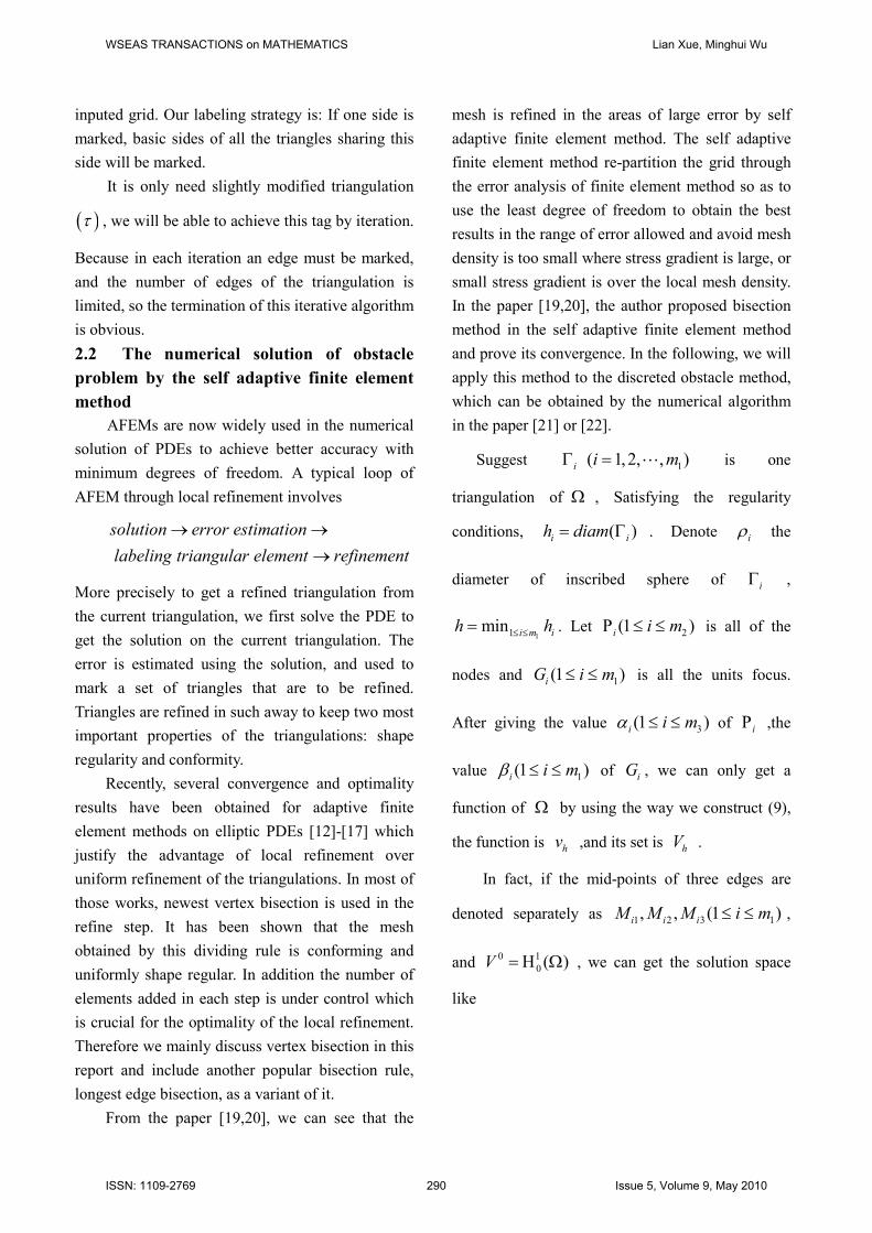
differential problem:

Suggest: 10 0 1, 0x y x yΩ = + < − ≤ ≤ = ,

finding the solution of the possion equation:

1 2,D

uu f in u u on g on

n

∂−∆ = Ω = Γ = Γ

∂ ,

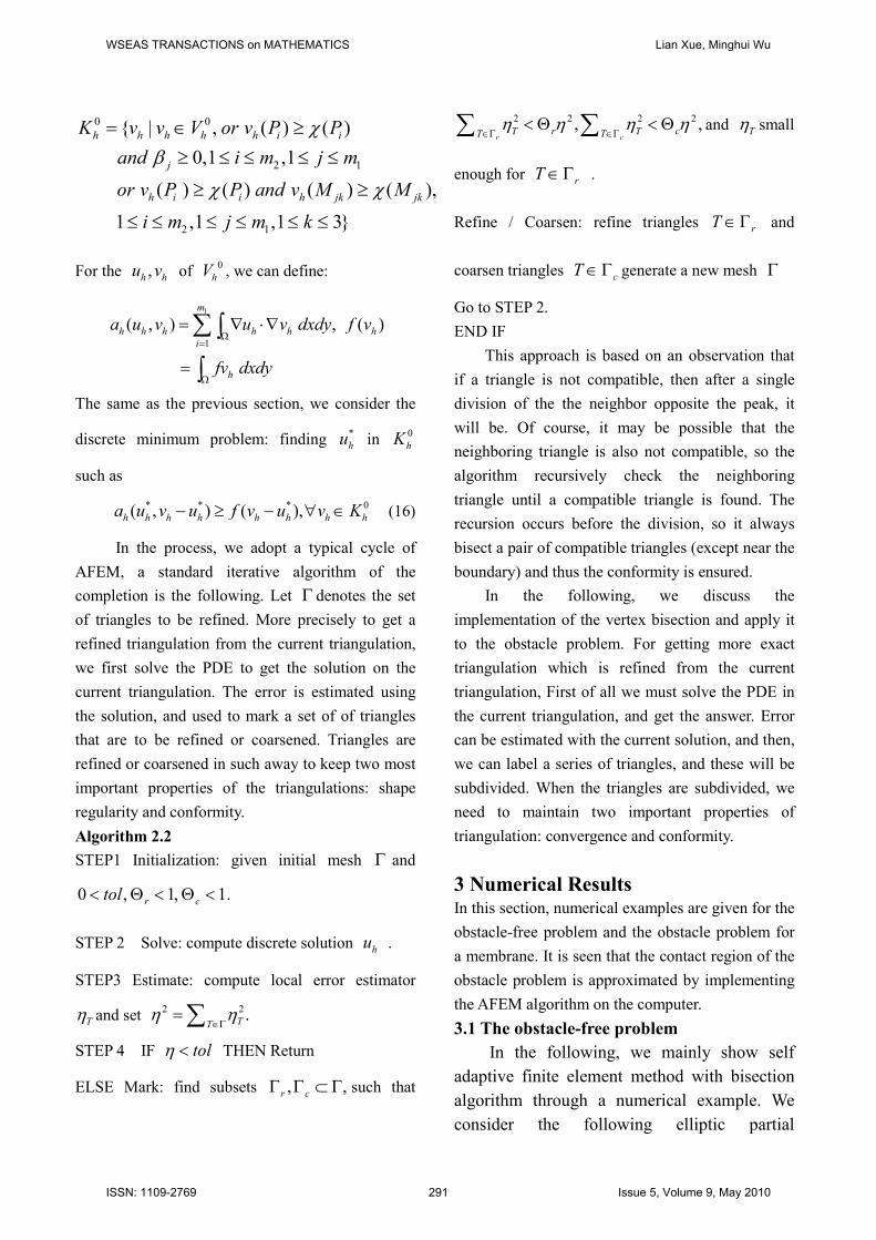
here 1 21, ,f = Γ = ∂Ω Γ = ∅ . The following

Fig.2 and Fig.3 are the solution graphics by a

different number of iterations in MATLAB.

-1

-0.5

0

0.5

1-1

-0.50

0.51

0

0.05

0.1

0.15

0.2

-1

-0.5

0

0.5

1-1

-0.5

0

0.5

1

Fig. 2: Numerical solution of obstacle-free problem

after 5 iterations

-1

-0.5

0

0.5

1-1

-0.50

0.51

0

0.05

0.1

0.15

0.2

-1

-0.5

0

0.5

1-1

-0.5

0

0.5

1

Fig. 3: Numerical solution of obstacle-free problem

after 10 iterations

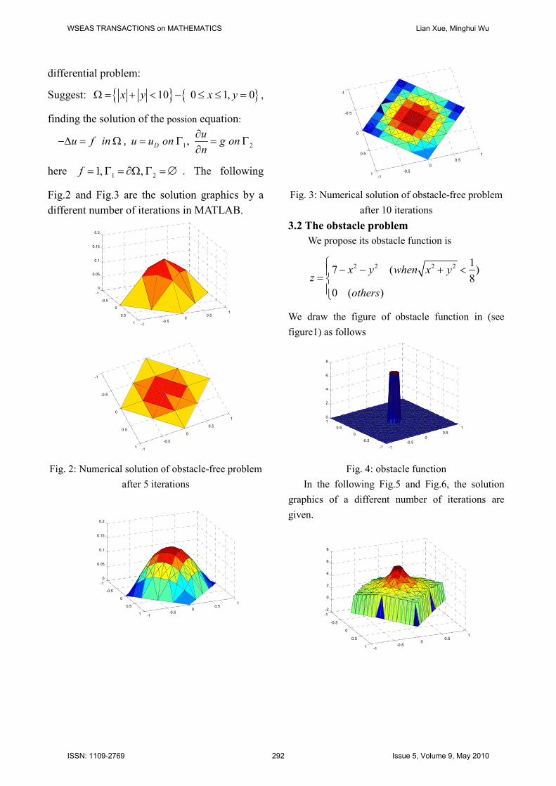
3.2 The obstacle problem

We propose its obstacle function is

2 2 2 2 17 ( )

8

0 ( )

x y when x yz

others

− − + <=

We draw the figure of obstacle function in (see

figure1) as follows

-1

-0.5

0

0.5

1

-1

-0.5

0

0.5

1

0

2

4

6

8

Fig. 4: obstacle function

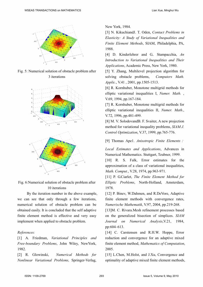
In the following Fig.5 and Fig.6, the solution

graphics of a different number of iterations are

given.

-1

-0.5

0

0.5

1-1

-0.50

0.51

-2

0

2

4

6

8



-1

-0.5

0

0.5

1-1

-0.5

0

0.5

1

Fig. 5: Numerical solution of obstacle problem after

3 iterations

-1

-0.5

0

0.5

1-1

-0.50

0.51

-2

0

2

4

6

8

-1

-0.5

0

0.5

1-1

-0.5

0

0.5

1

Fig. 6:Numerical solution of obstacle problem after

10 iterations

By the iteration number in the above example,

we can see that only through a few iterations,

numerical solution of obstacle problem can be

obtained easily. It is concluded that the self adaptive

finite element method is effective and very easy

implement when applied to obstacle problem.

References:

[1] A. Friedman, Variational Principles and

Free-boundary Problems, John Wiley, NewYork,

1982.

[2] R. Glowinski, Numerical Methods for

Nonlinear Variational Problems, Springer-Verlag,

New York, 1984.

[3] N. KikuchiandJ. T. Oden, Contact Problems in

Elasticity: A Study of Variational Inequalities and

Finite Element Methods, SIAM, Philadelphia, PA,

1988.

[4] D. Kinderlehrer and G.. Stampacchia, An

Introduction to Variational Inequalities and Their

Applications, Academic Press, New York, 1980.

[5] Y. Zhang, Multilevel projection algorithm for

solving obstacle problems, Computers Math.

Applic., V.41 , 2001, pp.1505-1513.

[6] R. Kornhuber, Monotone multigrid methods for

elliptic variational inequalities I, Numer. Math. ,

V.69, 1994, pp.167-184.

[7] R. Kornhuber, Monotone multigrid methods for

elliptic variational inequalities II, Numer. Math.,

V.72, 1996, pp.481-499.

[8] M. V. SolodovandB. F. Svaiter, A new projection

method for variational inequality problems, SIAM J.

Control Optimization, V.37, 1999, pp.765-776.

[9] Thomas Ape1. Anisotropic Finite Elements：

Local Estimates and Applications, Advances in

Numerical Mathematics. Stuttgart, Teubner, 1999.

[10] R. S. Falk, Error estimates for the

approximation of a class of variational inequalities,

Math. Comput., V.28, 1974, pp.963-971.

[11] P. G.Ciarlet, The Finite Element Method for

Elliptic Problems, North-Holland, Amsterdam,

1978.

[12] P. Binev, W.Dahmen, and R.DeVore, Adaptive

finite element methods with convergence rates,

Numerische Mathematik, V.97, 2004, pp.219-268.

[13]M. C. Rivara.Mesh refinement processes based

on the generalized bisection of simplices. SIAM

Journal on Numerical Analysis,V.21, 1984,

pp:604–613.

[14] C. Carstensen and R.H.W. Hoppe, Error

reduction and convergence for an adaptive mixed

finite element method, Mathematics of Computation,

2005.

[15] L.Chen, M.Holst, and J.Xu, Convergence and

optimality of adaptive mixed finite element methods,



Mathematics of Computation, V.78, 2009, pp.35-53.

[16] K.Mekchay and R.Nochetto, Convergence of

adaptive finite element methods for general second

or derlinear elliptic PDE, SIAM Journal on

Numerical Analysis, V.43, 2005, pp.1803-1827.

[17] P. Morin, R.H.Nochetto, and K.G.Siebert,

Convergence of adaptive finite element methods,

SIAM Review, V.44, 2002, pp.631-658.

[18] M. C. Rivara and GIribarren, The 4-triangles

longest-side partition of triangles and linear

renement algorithms, Mathematics of Computation,

V.65, 1996, pp.1485-1501.

[19] M.C.Rivara and M.Venere, Cost analysis of the

longest-side(triangle bisection) renement algorithms

for triangulations, Engineering with Computers,

V.12, 1996, pp.224-234.

[20]I. G. Rosenberg and F. Stenger. A lower bound

on the angles of triangles constructed by bisecting

the longest side. Mathematics of Computation, V.29,

1975, pp:390–395.

[21] X.L.Cheng, L.Xue,On the error estimate of

finite element dierence method for the obstacle

problem, Applied Mathematics and Computation,

V.183, 2006, pp.416-422.

[22] L.Xue, A New Iteration algorithm for the

obstacle problems,WSEAS Transactions on

Computers, V.6, 2007, pp.929-935.



Documents

The Numerical Solution of Obstacle Problem by … Numerical Solution of Obstacle Problem by Self Adaptive Finite Element Method LIAN XUE, MINGHUI WU* Schood of Computer and Computing