The Oilspill Risk Analysis Modelof the U.S. Geological Survey

G E O L O G I C A L S U R V E Y P R O F E S S I O N A L P A P E R 1 2 2 7

The Oilspill Risk Analysis Modelof the U.S. Geological Survey

By RICHARD A. SMITH, JAMES R. SLACK, TIMOTHY WYANT, a n dKENNETH J. LANFEAR

G E O L O G I C A L S U R V E Y P R O F E S S I O N A L P A P E R 1 2 2 7

I

U N I T E D S T A T E S G O V E R N M E N T P R I N T I N G O F F I C E , W A S H I N G T O N : 1 9 8 2

UNITED STATES DEPARTMENT OF THE INTERIOR

JAMES G. WATT, Secretary

GEOLOGICAL SURVEY

Dallas L. Peck, Director

For sale by the Branch of Distribution, U.S. Geological Survey.604 South Pickett Street. Alexandria, VA 22304

C O N T E N T S

FlbLRt 1-3

l, !,<

I L L U S T R A T I O N S

IV CONTENTS

TABLES

Page

b.7

8.[)

10.

st. qrTIc IIl In 30da Ys5 Output Iron) f)roqrdm FIR Sl” P.kS .Ave[aqe min imum. maximum, and mean [Imes-of-l ravel for oilspills occurring at s]te PI to contact

pru<r?s .

Li\tc]l rep,> rtsprepared for O(:Slcase stilranal\ sc'susiriq rllr(J)lsplll R1sk.Analysis Nlc>del.

Est[n)ate[i, oncijr L(>nalprr>t]abil i[]es.~nd txpcccedn ur~lt>er< ]lsp1lislarqcrthan l, OOOt)arrels reaching shore asaresult ofpe[roleun] develop.

METRIC CONVERSION FACTORS

S1 (International System of Units) is a modernized metric system of measurement. An asterisk after the last digit of the factorindicates that the conversion factor is exact and that all subsequent digits are zero, all other conversion factors have beenrounded to four significant digits.

To convert from — To Multiply by

inch (in) millimeter (mm) 25.4*foot (ft) meter (m) 0.3048mile (mi) kilometer (km) 1.609nautical mile kilometer (km} 1.852*acre m e t e r 2 ( mz) 4,047mile2 (m2) kilometer2 (km2) 2.590gallon (gal) meter 3 (m3) 0.003785barrel (bbl) meter3 (m3) 0.1590

(petroleum,1 bbl = 42 gal)

million gallons meter’ per second (m3/s) 0.04381per day (Mgal/d)

44

20

21

22

23

29

29

31

33

THE OILSPILL RISK ANALYSIS MODELOF THE U.S. GEOLOGICAL SURVEY

B y R I C H A R D A . SM I T H, JA M E S R . SL A C K,

T I M O T H Y W Y A N T, a n d KE N N E T H J . LA N F E A R

ABSTRACT

The U.S. Geological Survey has developed an oilspill risk analysismodel to aid in estimating the environmental hazards of developingoil resources in Outer Continental Shelf (OCS) lease areas. The large.computerized model analyzes the probability of spill occurrence, aswell as the likely paths or trajectories of spills in relation to the loca-tions of recreational and biological resources which may be vulner-able. The analytical methodology can easily incorporate estimatesof weathering rates, stick dispersion, and possible mitigating effectsof cleanup.

The probability of spill occurrence is estimated from informationon the anticipated level of oil production and method and route oftransport. Spill movement is modeled in Monte Carlo fashion with asample of 500 spills per season, each transported by monthly sur-face-current vectors and wind velocities sampled from 3-hour wind-transition matrices. Transition matrices are based on historic windrecords grouped in 41 wind velocity classes, and are constructedseasonally for up to six wind stations. Locations and monthly vul-nerabilities of up to 31 categories of environmental resources are di-gitized within an 800,000 km2 study area. Model output includestables of conditional impact probabilities (that is, the probability ofhitting a resource, given that a spill has occurred), as well as proba-bility distributions for oilspills occurring and contacting environ-mental resources within preselected vulnerability time horizons.

The model provides the U.S. Department of the Interior with amethod for realistically assessing oilspill risks associated with OCSdevelopment. To date, it has been used in oilspill risk assessmentsfor eight OCS lease sales with the results reported in Federal envi-ronmental impact statements. .4 summary of results is presentedherein. A ‘<real time” version was also used to forecast the move-ment of oil from the 1976-77 Argo Merchant oilspill. Additionalmodel runs are planned for future OCS lease sales in frontier areas,Other possible applications include analysis of OCS development al-ternatives and site selection for oilspill cleanup equipment.

I N T R O D U C T I O N

The past decade has been a period of rapid growth inthe offshore petroleum industry. The Department ofthe Interior currently conducts sales of mineral leases

for specific areas of the Outer Continental Shelf at therate of more than two per year, and it is anticipatedthat lease sales will continue, perhaps even at an in-creased rate, well into the 1980’s.

Oilspills are one of the major concerns associatedwith offshore oil development in all OCS lease saleareas. Concern is clearly strongest among those wholive in coastal areas and who depend, directly or in-directly, on coastal zone resources other than oil for alivelihood. Controversy over the risks and benefits ofoff-shore oil development inevitably gives rise to aneed for quantitative estimates of the oilspill risk in-volved in a particular development proposal. Withinthe Federal Government, oilspill risk estimates are re-quired prior to holding an OCS lease sale, at the timethe Secretary of the Interior makes decisions on tractsto be withheld from leasing because of unacceptableoilspill risk to specific environmental resources in theproposed sale area. At issue in the decisionmaking fora typical OCS lease sale are anywhere from 100 to 500nine-square-mile tracts which have been identified aspossible production areas by interested oil companies.Also at issue areas many as 20 or 30 specific resourceswhich have been identified by the Bureau of LandManagement or the U.S. Geological Survey as vulner-able to oilspills on the basis of research and communi-cation with local authorities.

An important fact that stands out when one at-tempts to predict oilspill damages for a proposed OCSlease area is that the problem is fundamentally proba-bilistic. A great deal of uncertainty exists not onlywith regard to the location, number, and size of spillsthat will occur during the course of development, butalso with regard to the wind and current conditionsthat will exist and give direction to the oil at the partic-ular times spills occur. While some of the uncertainty

1

2 OILSPILL RISK ANALYSIS MODEL OF U.S. GEOLOGICAL SURVEY

reflects incomplete or imperfect data, considerable un-certainty is simply inherent in the problem.

The Geological Survey has developed a model for as-sessing the oilspill risks associated with petroleum de-velopment in Federal OCS lease areas. The model isconstructed to deal with three fundamental and essen-tially independent factors which comprise the total oil-spill risk to coastal zone resources: ( 1 ) the probabilityof spill occurrence as a function of the quantity of oilwhich is to be produced and handled at individual pro-duction sites, pipelines, and tanker routes; (2) the prob-abilities of occurrence of various spill trajectories fromproduction sites and transportation routes as a func-tion of historical wind and current patterns for thearea: and (3) the location in space and time of vulner-able resources defined according to the same coordin-ate system used in spill trajectory simulation. Resultsof the individual parts of the analysis are combined toestimate the total oilspill risk associated with produc-tion and transportation at locations within a proposedlease area. This information is then used in making fi-nal tract selections prior to leasing. To date, risk analy-ses have been conducted for seven Federal lease areas,including sites offshore the North-, Mid-, and South-Atlantic Coasts, the Eastern Gulf of Mexico, SouthernCalifornia, and the Western and Northern Gulf of Alas-ka.

The purpose of this report is to describe how the Oil-spill Risk Analysis Model of the U.S. Geological Sur-vey works, both in theory and in actual operation. Itdiscusses the assumptions used in developing the mod-el and defines the role of each computer program.While not a detailed operating instruction manual, itprovides the broad understanding of the model whichis necessary for operating the model and properly in-terpreting the results.

The report begins with a discussion of how the database is developed, proceeds to describe how oilspillsare simulated, and then reviews the results to date.The section, “Representations of Physical Data,”’ des-cribes how winds, currents, and the locations of envi-ronmental resources, or targets, are represented as da-ta and put in the proper form for analysis. Simulationof oilspill movement is the topic of the section, “Oil-spill Trajectory Simulation,” and the probabilistic cal-culations of oilspill risk is covered in “Risk Calcula-tion.” The section, “Model Verification and Limita-tions,” places the accuracy of risk calculations in per-spective with discussions of sensitivity and verifica-tion studies. A summary of past results and ideas forfuture uses of the model are presented in the section,“Model Output and Case Examples." Discussion of“Practical Aspects of Operating and Managing theModel” concludes the paper.

REPRESENTATIONS OF PHYSICAL DATA

The model of the U.S. Geological Survey is designedto use a large amount of information about the physi-cal environment, including sizable files of wind andcurrent data and the locations of numerous environ-mental resources which may be adversely affected byoilspills. Model programs process all of this data andstore it in computer files before any trajectories arecomputed. All of the files are designed to allow rapidaccess to the data by subsequent computer programs.An extensive system of internal checks, along withgraphic displays and printouts, help ensure that physi-cal data are represented correctly. The following sec-tion describes how physical data are collected, pro-cessed, checked, and stored.

BASE MAP

A system for representing spatial locations is thefoundation of the trajectory simulation model. The mo-del employs a Cartesian coordinate system superim-posed over a base map of the study area. All stored da-ta are referenced to this system, and it is used for all in-ternal calculations.

The initial step in establishing a coordinate systemis the delineation of the area to be modeled. This areamust be large enough so that all oilspill targets likelyto be affected, such as land or biological resources, areincluded; at the same time, the map scale must not beso large that essential details are obscured. PreviousOCS lease sale analyses have typically examined areasof about 800 km by 800 km, and included 1,000 km ofcoastline. The base map boundaries are usually chosenso that the major origins of potential spills, such as thelease area and transportation routes, are centered; ifwinds or currents are expected to drive spills predomi-nantly in a certain direction, the map is shifted accord-ingly. Land need only be included to the extent neces-sary to define the shoreline, and to aid in visual recog-nition of the map.

Choice of a projection for the base map is particular-ly important, since representing the surface of theearth by a planar surface necessarily introduces somedistortion in scale, or direction, or both. The UniversalTransverse Mercator (UTM) projection system has rel-atively little scale distortion but has a directional dis-tortion of about 10 degrees. Because the equations forcorrecting this distortion are lengthy and too expen-sive to perform for each trajectory movement, earlierOCS lease sale analyses used UTM or Lambert projec-tions and neglected distortion. However, neglectingdistortion caused serious difficulties in combining dataobtained from different maps, and necessitated use ofa more general mapping system.

REPRESENTATIONS OF PHYSICAL. DATA 3

A useful property of the Mercator projection is thatthere is no distortion in direction; that is, a constantcompass direction is a straight line. This makes it ex-tremely easy to align a Mercator projection with a Car-tesian coordinate system. The penalty for this, how-ever, is extreme distortion in scale, particularly at highlatitudes. Fortunately, the correction factor is a rela-tively simple function of latitude, which the computercan calculate quickly and easily. Because of theseproperties, the Mercator projection is ideal for oilspillmodeling purposes, and is now used by the modelwhenever possible.

Once the base map has been selected, a Cartesian co-ordinate system is superimposed with its origin at thelower left-hand (southwest) corner of the map. Thelongest side of the map is usually assigned a length of480 units. The whole study area is then divided into amatrix of square cells of one unit each; the maximumsize of this matrix is 480X480 cells. For a typical an-alysis, each cell represents an area of approximately 2to 4 km’, which is thus the basic unit of resolution forspatial data.

Spatial data is stored in a set of 480x480 matrices.Elements of the matrices define, for every cell:

. Presence or absence of land, and land segments.● Presence or absence of up to 31 targets,. Identification of a wind station, for determining

the appropriate wind vector for oilspill move-ment (see subsection-Wind Data).

● Identification of a current polygon, for determin-ing the appropriate current vector for oilspillmovement (see subsection—Current DataChecking).

Processing data to construct large arrays is a compli-cated task requiring a great deal of automation. Like-wise, the practical limitations of computers require anefficient, though sometimes complex, storage and pag-ing scheme for handling these matrices. Other sectionsdescribe the matrices in “more detail.

LAND AND TARGETS

One primary function of the model is to relate oilspilltrajectory movements to the locations of wildlife popu-lations, fishing areas, and other potential “targets” incoastal and continental shelf areas. Environmental im-pact statements for Federal OCS leasing require col-lecting an enormous quantity of data about these re-sources, and a substantial part of this data basebecomes input for the model.

STORAGE OF TARGETS

T h e m o d e l s t o r e s i n d i c a t o r s o f t h e p r e s e n c e o rabsence of land and up to 31 other targets in each of a

quarter million grid cells. This is done in such a waythat each of perhaps 150,000 simulated spills arequickly checked at each step in the trajectory for possi-ble impact on each target.

Two features of the model allow a high level of per-formance in checking cells. When trajectories are beingsimulated by program SPILL (see section on "OilspillMovement,”) a paging system burdens computermemory with only a small, easily accessible fraction ofthe total grid at any time. Additionally, an effective ex-ploitation of IBM storage attributes provides a com-pact and efficient mechanism for handling data whichresides either in main memory or on permanent storagedevices.

More technically, each grid cell is assigned one4-byte integer to indicate the presence of up to 31categories of targets, and land. Each of the 32 bits(numbered O-31) corresponds to a different target, orland. Bit O, the sign bit, corresponds to land, and is“on” when land is present in the cell. Bit i representsthe target number i and the interger value 2**(3l-i);“on” signals that the target is present in the cell. Thusan integer value of, say, 9 (binary 000000000000000000000000 00001001) would indicate that targets 28and 31 are present. Simple subroutines can decodethese integers to suit various purposes.

TYPES OF TARGETS

Examples of spill-vulnerable targets which have beenincluded in past analyses appear in tables 1 and 2.Sample targets are shown in figures 1 and 2. A simu-lated spill registers either “hit” or’ ‘no hit” on a target.A hit is scored as soon as the simulated spill crosses acell occupied by the target. Multiple crossings by thesame spill count as a single hit.

The selection of targets is clearly of critical impor-tance if the model is to produce useful results, The sec-tion, “Model Output and Case Examples” further dis-cusses the targets considered in past risk analyses.

FURTHER REFINEMENTS OF TARGETS-SEASONAL VULNERABILITY

Passage of spilled oil through a target location doesnot necessarily imply an adverse impact on the target,since vulnerability of a single target may vary accor-ding to time of year. Many wildlife populations under-go migrations during the year, and seasonal reproduc-tive activities are often more susceptible to damagefrom spilled oil than other parts of the life cycle, Theeconomic impact of spilled oil on such targets asbeaches may also differ seasonally.

4 OILSPILL. RISK ANALYSIS MODEL OF THE U.S. GEOLOGICAL SURVEY

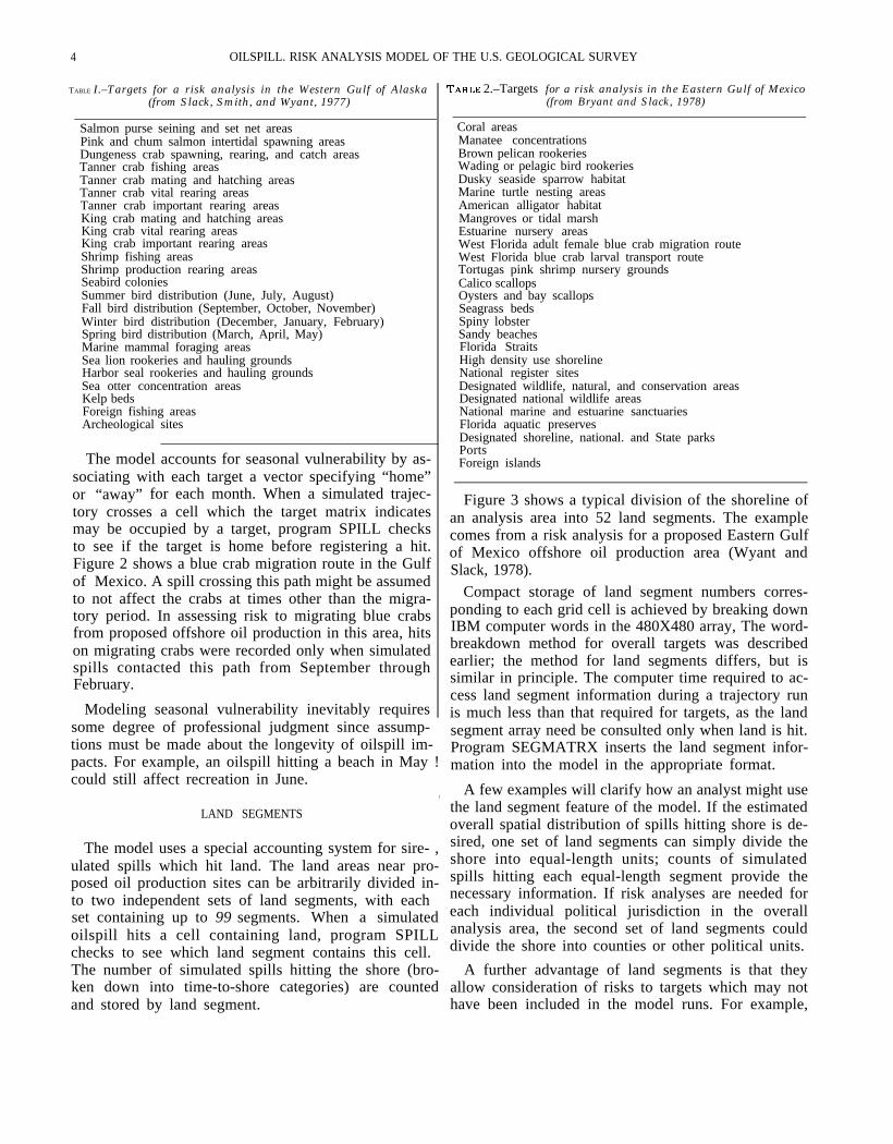
TABLE I.–Targets for a risk analysis in the Western Gulf of Alaska(from Slack, Smith, and Wyant, 1977)

Salmon purse seining and set net areasPink and chum salmon intertidal spawning areasDungeness crab spawning, rearing, and catch areasTanner crab fishing areasTanner crab mating and hatching areasTanner crab vital rearing areasTanner crab important rearing areasKing crab mating and hatching areasKing crab vital rearing areasKing crab important rearing areasShrimp fishing areasShrimp production rearing areasSeabird coloniesSummer bird distribution (June, July, August)Fall bird distribution (September, October, November)Winter bird distribution (December, January, February)Spring bird distribution (March, April, May)Marine mammal foraging areasSea lion rookeries and hauling groundsHarbor seal rookeries and hauling groundsSea otter concentration areasKelp bedsForeign fishing areasArcheological sites

The model accounts for seasonal vulnerability by as-sociating with each target a vector specifying “home”or “away” for each month. When a simulated trajec-tory crosses a cell which the target matrix indicatesmay be occupied by a target, program SPILL checksto see if the target is home before registering a hit.Figure 2 shows a blue crab migration route in the Gulfof Mexico. A spill crossing this path might be assumedto not affect the crabs at times other than the migra-tory period. In assessing risk to migrating blue crabsfrom proposed offshore oil production in this area, hitson migrating crabs were recorded only when simulatedspills contacted this path from September throughFebruary.

Modeling seasonal vulnerability inevitably requiressome degree of professional judgment since assump-tions must be made about the longevity of oilspill im- pacts. For example, an oilspill hitting a beach in May !could still affect recreation in June.

,LAND SEGMENTS

The model uses a special accounting system for sire- ,ulated spills which hit land. The land areas near pro-posed oil production sites can be arbitrarily divided in-to two independent sets of land segments, with eachset containing up to 99 segments. When a simulatedoilspill hits a cell containing land, program SPILLchecks to see which land segment contains this cell. The number of simulated spills hitting the shore (bro-ken down into time-to-shore categories) are countedand stored by land segment.

T.A~ LE 2.–Targets for a risk analysis in the Eastern Gulf of Mexico(from Bryant and Slack, 1978)

Coral areasManatee concentrationsBrown pelican rookeriesWading or pelagic bird rookeriesDusky seaside sparrow habitatMarine turtle nesting areasAmerican alligator habitatMangroves or tidal marshEstuarine nursery areasWest Florida adult female blue crab migration routeWest Florida blue crab larval transport routeTortugas pink shrimp nursery groundsCalico scallopsOysters and bay scallopsSeagrass bedsSpiny lobsterSandy beachesFlorida StraitsHigh density use shorelineNational register sitesDesignated wildlife, natural, and conservation areasDesignated national wildlife areasNational marine and estuarine sanctuariesFlorida aquatic preservesDesignated shoreline, national. and State parksPortsForeign islands

Figure 3 shows a typical division of the shoreline ofan analysis area into 52 land segments. The examplecomes from a risk analysis for a proposed Eastern Gulfof Mexico offshore oil production area (Wyant andSlack, 1978).

Compact storage of land segment numbers corres-ponding to each grid cell is achieved by breaking downIBM computer words in the 480X480 array, The word-breakdown method for overall targets was describedearlier; the method for land segments differs, but issimilar in principle. The computer time required to ac-cess land segment information during a trajectory runis much less than that required for targets, as the landsegment array need be consulted only when land is hit.Program SEGMATRX inserts the land segment infor-mation into the model in the appropriate format.

A few examples will clarify how an analyst might usethe land segment feature of the model. If the estimatedoverall spatial distribution of spills hitting shore is de-sired, one set of land segments can simply divide theshore into equal-length units; counts of simulatedspills hitting each equal-length segment provide thenecessary information. If risk analyses are needed foreach individual political jurisdiction in the overallanalysis area, the second set of land segments coulddivide the shore into counties or other political units.

A further advantage of land segments is that theyallow consideration of risks to targets which may nothave been included in the model runs. For example,

REPRE.SENTXIIOXS (>F PHYS1(:.A1. D A T A 5

1 —

I-Al

Ju

- G U L F O F A L A S K A

FIGURE 1.–.Map showing a sample target in the Western Gulf of Alaska. Hatched areas indicate foreign fishing areas.Rectangles are proposed lease tracts (Slack, et al, 19’77)

suppose that after the model has been run, a shorelinespecies is added to endangered species lists. Risk tothe species can be estimated by examining the landsegments in which the species resides.

Finally, the model is not applicable in many bays andestuaries. In a risk analysis for the Mid-Atlantic coast(Slack and Wyant, 1978), simulated spills were not per-mitted to enter the Chesapeake or Delaware estuarieswhere the trajectory assumptions of the model are notapplicable. To count simulated spills which would haveentered the bays, the bay entrances were treated asparts of the shoreline, and a land segment was associ-ated with each bay entrance. Counts of simulated spills

hitting these land segments allowed analysis of risk tothe bays as a whole without addressing the furtherproblems of spill movements within the bays.

CHECKING TARGETS AND LAND SEGMENT D\TA

The model is designed to allow treatment of exten-sive and intricate spatial information. In addition tocreating computer storage and run-time problems, thesize and complexity of the model’s basic data structurecreates validation problems. Inattention to errors in

data input can often lead to disastrously misleadingoutput. Given the time and tedium required for data

6 O[l,SPI1.I. R[SK .AX,AI.}’SIS N1ODEI. OF ‘1’HE L’ S. GEOI.OGIC.4L SCR1’Ei

GfJL

oL_L_ulYN A UT IC AL MIL ES

F o f ME

N

t

m v

C71-J

Xlco

TL ANTIC

O C E A N

FLGURE 2.–Map showing a sample target in the Eastern Gulf of Mexico. Hat,ched area indicates blue crab migration route.Rectangles are proposed lease tracts (Wyant and Slack, 1978),

checking and the greater intellectual satisfaction oftinkering with the analytical specifications of the mod-el, it is always tempting to pay too little attention tothis possibility. The computer programs have been de-signed to make data checking as complete and conven-ient as possible, and to prompt modelers to thoroughlycarry out this phase of an analysis. OBJECTS andother spatial data entry programs routinely providediagnostic information such as the number of points inthe overall grid system used to represent each target.A coded version of the array used to store the targetlocations is routinely printed in each run of OBJECTS.The most important checking routines, however, aregraphical.

Computer graphics provide a powerful tool for quick-ly and fully examining complex spatial data. This toolis exploited throughout the data entry phases of amodel run. Program DIGIPLOT plots each target as itresides on computer tape immediately after entry froma digitizer. (The target’s location at this stage is storedas a string of x-y coordinates representing locations

along the boundary of the target area on a map laid onthe plane of the digitizer table. See the next subsec-tion, “Insertion of Spatial Data into the Model, ” formore detail. ) Timely examination of freshly enteredspatial data using DIGIPLOT speeds the data entryphase of a model run and prevents costly cascading oferrors through subsequent programs.

When program OBJECTS has inserted target loca-tions into the final grid system, program OBJPLOTproduces plots such as figures 1 and 2. These plotsallow quick appraisal of how faithfully and completelytarget location in the final coordinate system agreeswith the target location on the original map. Theseplots also provide an immediate check on the correct-ness of the various map scalings, rotations, and projec-tions required to combine spatial information from dif-ferent maps and different sessions on the digitizer.

In addition to providing the key to thorough and eco-nomical data checking, these computer-graphics pro-grams are an invaluable tool for communicating thecontent and output of the Survey model. Model results

I+t. I’Rl sl, sI. \llo\s OF Pt{YslcA1. 1P. ].+

B

.0

G U L F

ol-u-l_dwNAUTICAL MILES

o f

4/’24F L O

25.-

[-34

30

I

LA,V TIC

O C E A N

—

-

I

FIGURE 3.–Map showing a typical division of the shoreline into land segments (Wyant and Slack, 1978).

must often be presented to users from a variety of tech-nical backgrounds. Pictures such as figures 1 and 2 areeasily understood.

INSERTION OF SPATIAL DATA INTO THE MODEL

This subsection describes the mechanical details ofinserting spatial data into the model.

Target location is originally provided on a map ofpart of the overall analysis area. Each map must havea pair of reference points corresponding to a pair of ref-erence points on the overall map of the area.

The map is laid on a digitizer table, and the outline ofa target is traced with the digitizers electrical cross-hairs. This converts the image of the outline to a se-quence of points expressed in digitizer table coordin-ates. The digitizer stores this sequence of coordinateson computer tape.

Program DIGIPRE screens the digitized locationsof reference points, targets, and shorelines and storesthem on a direct access disk pack in a form accessible

to program OBJECTS. Program DIG I PLOT createsdiagnostic plots of target locations from these diskfiles to check against the original maps.

Several options are available for entering spatialdata. Correct use of the options speeds the entry pro-cess and simplifies data organization and storage. Pro-grams DIG I PLOT and OBJECTS automaticallycheck for large gaps in the point sequences represen-ting target outlines. Thus, the outline of a target withmany discrete subareas, such as an island chain, can betraced on the digitizer table and the model will auto-matically recognize the individual islands. Targetsrepresentable as polygons can be entered simply bydigitizing the polygon vertices; they need not be tracedin their entirety. Some targets can also be entered asisolated points, but this presents some theoretical dif-ficulties, since oilspills are also represented as points.

Land segments are entered much the same as poly-gonal targets. The order in which the polygon verticesare digitized is important—a specific order is needed to

8 011. S1’11.1. RISK .AX.AI.YSIS \loDEL {)F THE U S GEOLOGICAL SUR\’E}

let subsequent programs produce plots like figure 3.Land segments are stored somewhat differently fromoverall targets and are processed by programsDIGICOPY and SEGMATRX rather than OBJECTSand DIGIPRES.

OBJECTS performs several functions. The sequenceof points representing a target outline on the digitizertable is scaled, rotated, and projected into the finalcoordinate system. The grid cells occupied by thesepoints are noted, and the grid outline of the target iscompletely connected using subroutines GETLIM,NBR, and TRACK. The grid cells inside the outline arethen found using subroutine FILL. Grid locations ofthe targets, or segments, are compactly stored in ar-rays using the compaction methods described pre-viously. The arrays are then stored on a direct accessdisk in such a way that they are accessible to the tra-jectory program SPILL via subroutine NEWBLK’spaging system. They are also accessed by program OB-JPLOT, to produce drawings of the target locations, asin figures 1 and 2. SEGMATRX performs an identicalfunction for land segments.

PAGING SYSTEM FOR LARGE ARRAYS

The 480 X 480 arrays identifying targets and landsegments occupy almost 1.4 megabytes of storage.Since only a small portion of each array is needed atany time, a paging system has proven economical in re-ducing computer core requirements.

Each large array is divided into 30X 30 blocks,which are stored as direct-access records on a disk. Thepaging system will retain the most recently usedblocks in core, and access the others as needed. A fur-ther refinement for the array of targets is to constructa 16 X 16 array (one element for each block of the tar-get array) that indicates presence or absence of targetcategories in each of the blocks. Thus, by checking thesmaller array, the computer can determine whether ornot it is necessary to read a block of the larger array.

WINDS

The subsections which follow explain how wind datais put into a form that can be used for oilspill simula-tion. Movement of oil under the influence of wind iscovered in "Oilspill Trajectory Simulation.”

STO~H.\STIC 510 DEL O F M“l SD D.\TA

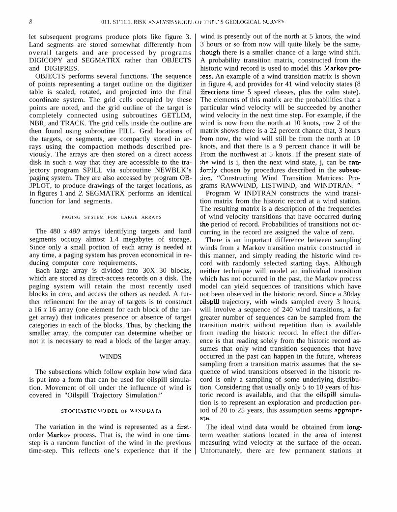
The variation in the wind is represented as a first-order Markov process. That is, the wind in one time-step is a random function of the wind in the previoustime-step. This reflects one’s experience that if the

wind is presently out of the north at 5 knots, the wind3 hours or so from now will quite likely be the same,though there is a smaller chance of a large wind shift.A probability transition matrix, constructed from thehistoric wind record is used to model this Markov pro-:ess. An example of a wind transition matrix is shownin figure 4, and provides for 41 wind velocity states (8~irections time 5 speed classes, plus the calm state).The elements of this matrix are the probabilities that aparticular wind velocity will be succeeded by anotherwind velocity in the next time step. For example, if thewind is now from the north at 10 knots, row 2 of thematrix shows there is a 22 percent chance that, 3 hoursfrom now, the wind will still be from the north at 10knots, and that there is a 9 percent chance it will beFrom the northwest at 5 knots. If the present state of:he wind is i, then the next wind state, j, can be ran-~omly chosen by procedures described in the subsec-tion, “Constructing Wind Transition Matrices: Pro-grams RAWWIND, LISTWIND, and WINDTRAN. ”

Program W INDTRAN constructs the wind transi-tion matrix from the historic record at a wind station.The resulting matrix is a description of the frequenciesof wind velocity transitions that have occurred duringthe period of record. Probabilities of transitions not oc-curring in the record are assigned the value of zero.

There is an important difference between samplingwinds from a Markov transition matrix constructed inthis manner, and simply reading the historic wind re-cord with randomly selected starting days. Althoughneither technique will model an individual transitionwhich has not occurred in the past, the Markov processmodel can yield sequences of transitions which havenot been observed in the historic record. Since a 30dayoilspill trajectory, with winds sampled every 3 hours,will involve a sequence of 240 wind transitions, a fargreater number of sequences can be sampled from thetransition matrix without repetition than is availablefrom reading the historic record. In effect the differ-ence is that reading solely from the historic record as-sumes that only wind transition sequences that haveoccurred in the past can happen in the future, whereassampling from a transition matrix assumes that the se-quence of wind transitions observed in the historic re-cord is only a sampling of some underlying distribu-tion. Considering that usually only 5 to 10 years of his-toric record is available, and that the oilspill simula-tion is to represent an exploration and production per-iod of 20 to 25 years, this assumption seems appropr-iate.

The ideal wind data would be obtained from long-term weather stations located in the area of interestmeasuring wind velocity at the surface of the ocean.Unfortunately, there are few permanent stations at

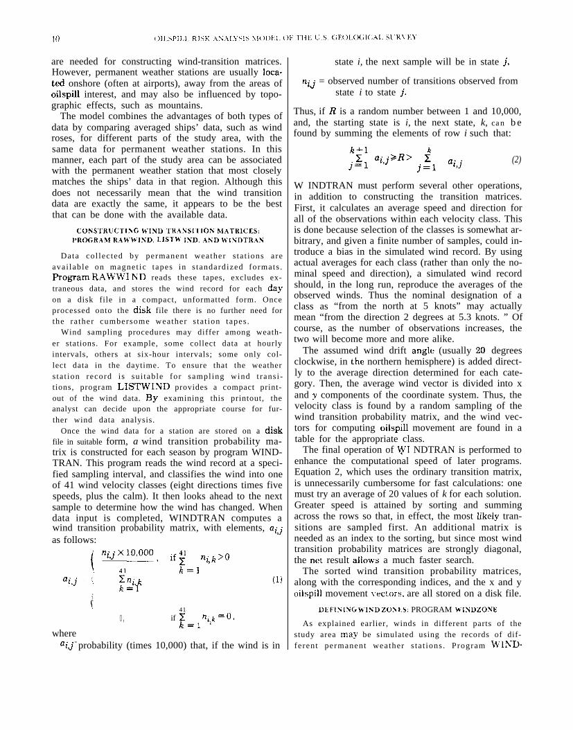
are needed for constructing wind-transition matrices.However, permanent weather stations are usually loca-ted onshore (often at airports), away from the areas ofoilspill interest, and may also be influenced by topo-graphic effects, such as mountains.

The model combines the advantages of both types ofdata by comparing averaged ships’ data, such as windroses, for different parts of the study area, with thesame data for permanent weather stations. In thismanner, each part of the study area can be associatedwith the permanent weather station that most closelymatches the ships’ data in that region. Although thisdoes not necessarily mean that the wind transitiondata are exactly the same, it appears to be the bestthat can be done with the available data.

CO~STRUCTIYG wI~D TR.4~S1TI05/ L1.4TR1CES:PROGR.4\f R.4~~ISD. LISTw I~D. AND ~I?4DTR.A~

Data col lec ted by permanent weather s ta t ions areavai lable on magnet ic tapes in s tandardized formats .ProgTam RAWW1 ND reads these tapes, excludes ex-traneous data, and stores the wind record for each dayon a disk file in a compact, unformatted form. Onceprocessed onto the disk file there is no further need forthe ra ther cumbersome weather s ta t ion tapes .

Wind sampling procedures may differ among weath-er stations. For example, some collect data at hourlyintervals, others at six-hour intervals; some only col-lect data in the daytime. To ensure that the weathers ta t ion record i s su i table for sampl ing wind t rans i -tions, program LISTWIND provides a compact print-out of the wind data. By examining this printout, theanalyst can decide upon the appropriate course for fur-ther wind data analysis.

Once the wind data for a station are stored on a diskfile in suitable form, a wind transition probability ma-trix is constructed for each season by program WIND-TRAN. This program reads the wind record at a speci-fied sampling interval, and classifies the wind into oneof 41 wind velocity classes (eight directions times fivespeeds, plus the calm). It then looks ahead to the nextsample to determine how the wind has changed. Whendata input is completed, WINDTRAN computes awind transition probability matrix, with elements, ai,jas follows:

( n~,j x 10,000, nik>()if? ~\ 41 k=]

ai,j = ‘,, ~Tli,k

ik=l

(1)

\ 41

0, if ~ Tllk=O,k=l ‘

whereai,~ = probability (times 10,000) that, if the wind is in

state i, the next sample will be in state j,

“ . = observed number of transitions observed from‘l,J

state i to state j.

Thus, if R is a random number between 1 and 10,000,and, the starting state is i, the next state, k, can b efound by summing the elements of row i such that:

k+l~ ~i,j>R> ~

‘ijjj=l j=l(2)

W INDTRAN must perform several other operations,in addition to constructing the transition matrices.First, it calculates an average speed and direction forall of the observations within each velocity class. Thisis done because selection of the classes is somewhat ar-bitrary, and given a finite number of samples, could in-troduce a bias in the simulated wind record. By usingactual averages for each class (rather than only the no-minal speed and direction), a simulated wind recordshould, in the long run, reproduce the averages of theobserved winds. Thus the nominal designation of aclass as “from the north at 5 knots” may actuallymean “from the direction 2 degrees at 5.3 knots. ” Ofcourse, as the number of observations increases, thetwo will become more and more alike.

The assumed wind drift angle (usually 20 degreesclockwise, in the northern hemisphere) is added direct-ly to the average direction determined for each cate-gory. Then, the average wind vector is divided into xand y components of the coordinate system. Thus, thevelocity class is found by a random sampling of thewind transition probability matrix, and the wind vec-tors for computing oilspill movement are found in atable for the appropriate class.

The final operation of ~1 NDTRAN is performed toenhance the computational speed of later programs.Equation 2, which uses the ordinary transition matrix,is unnecessarily cumbersome for fast calculations: onemust try an average of 20 values of k for each solution.Greater speed is attained by sorting and summingacross the rows so that, in effect, the most likely tran-sitions are sampled first. An additional matrix isneeded as an index to the sorting, but since most windtransition probability matrices are strongly diagonal,the net result allows a much faster search.

The sorted wind transition probability matrices,along with the corresponding indices, and the x and yoilspill movement \ectors, are all stored on a disk file.

DEFINING ~IXD ZO>ES: PROGRAM ~IXDZOSE

As explained earlier, winds in different parts of thestudy area may be simulated using the records of dif-ferent permanent weather s ta t ions . Program WIND-

()[1.>}’11.1. I’R,\,] E(YI’L)R’l’ sI\ful..i”l lox 11

ZONE assigns to each 10X lO block of grid cells aselected wind station number. By reading the wind sta-tion number, program SPILL can find the correct windstation L.o use for any location. Up to six sets of windtransition probability matrices, constructed from therecords of six permanent weather stations, are per-mitted. Figure 5 shows an example of wind zones usedfor OCS Lease Sale 48; this particular analysis usedfour weather stations.

CURRENTS

Ocean currents are represented in the model as vary--ing from month to month in a deterministic fashion.This is in contrast to the winds, which vary randomlyover a relatively short time period. Spatial variation ofcurrents is incorporated by dividing the study area in-to as many as 600 subareas, and assigning monthlycurrent vectors to each of these subareas.

The model does not actually model ocean currentsbut utilizes a current field determined by other means.Input data for currents, whether derived from mathe-matical models or from direct measurements, mustconform to the assumption (made in the preceding sec-tions) that winds and currents are uncorrelated withina given month. Therefore, the current field used for themodel is the baroclinic current, and all wind-inducedcurrents must be represented with the wind data.

Tidal currents are also not incIuded in the model.Generally, the waters in which tides are an importanttransport mechanism are not within the model’s in-tended scope of analysis.

CURRENT DATA ENTRY .41ND STORAGE:PROGRAMS CIJRPOLY AND CLJRMATRX

Current data are made available to the model frommaps of the study area showing the current field foreach month. The study area is then divided into sub-areas or polygons, with 600 the maximum number.Each polygon is assigned a current vector for everymonth. The polygons are, therefore, a finite-elementrepresentation of the current field.

The polygon configuration must be able to adequate-ly characterize the overall monthly current fields withthe fewest possible polygons, At present, the judg-ments of the analysts and modelers are the sole deter-minants of the polygon configuration for each analysis.lNo mechanical polygon construction routine exists.Figure 6 shows a monthly current field of 518 currentvectors used by the model in a run for a southernCalifornia risk analysis (see Slack, Wyant, and Lan-fear. 19781: figure 7 shows che 518 polygons.

The vertices of the current polygons are first digi-tized in the same manner as land segment polygons(see “Land and Targets’ ‘). Program DIG I COPY trans-

fers the digitized information into direct access diskdatasets. Program CURPOLY combines the informa-tion in these datasets into a single current polygon file.Program CURMATRX then carries out the final pro-cessing steps to make current data accessible to pro-gram SPILL: (1) The polygon vertices are scaled, ro-tated, and projected from digitizer table coordinates tothe final model coordinate system; (2) a 480 X 4802-byte integer array is filled with the current polygonidentification numbers corresponding to each grid cell:(3) this array is stored on a disk file accessible to pro-gram SPILL’s paging system; (4) the monthly currentvelocities associated with each polygon are read fromcards and stored in another disk file. CURMATRX al-so generates diagnostic plots for data checking and aprintout of the grid system showing the current poly-gon associated with each cell.

CURRENT DATA CHECKINGThe special requirements of the modeI and the occa-

sional need to obtain current data from several sourcesnecessitate the translation of large amounts of currentdata to the appropriate format at the beginning of eve-ry analysis. Several programs of the model enablequick and thorough graphical checking of the final-for-mat current data to detect translation errors. Graphicsare especially effective in detecting major errors. Pro-grams CURPLOT and CUR.MATRX provide plots ofpolygon locations, plots of spatial current fields, bymonth, and diagnostic printouts of the final 480 X 480current grid.

OILSPILL TRAJECTORY SIMULATIONMONTE CARLO SIMULATIONSOF OILSPILL TRAJECTORIES

For each selected launch point, a large number of hy-pothetical oilspills are released at randomly chosendays within the year and are moved about by randomlysampled winds and currents. With sufficient trials, thestatistical behavior of the trial spills will approximatethe statistical behavior of spills integrated over all pos-sible combinations of release times, winds, and cur-rents.

The model analyzes oilspill trajectories from a set ofpotential launch points which are chosen to representdifferent proposed oil production sites in the OCS leasearea and proposed transportation routes. A total of100 launch points may be selected. From each launchpoint, 500 hypothetical oilspills are simulated for eachseason of the year, resulting in as many as 200,000simulated oilspills for a model run, The next sectionshows how these simulation results are fur[her ana-lyzed to determine risks from various parts of the leasearea.

12 [)1 LSPIL1, RISK ,A\A[.>”SIS \lOl)E1, OF ‘1’HF; L’ S L; F:(JL(X; IC.A. L SL’R\’EY

-. SAN FRANCISCO

\

\ C A L I F O R N I A

PT’

--

P A C I F I C O C E A N

oU-l-L-d”NAUTICM MILES

{

*

M EXICO

FJ~ LRE .5. -~ind zones used for OCS Lease Sale 48–southern California. Four weather stations were used instead of six.Rectangles are proposed lease tracts (Slack, Wyant, and Lanfear, 19781,

A single Iaunch po in t may adequate ly por t ray a Igroup of proposed lease tracts, but additional pointsare of ten needed to represent p ipel ines and tankerroutes. An option of the model allows a launch point to

be specified as a straight line, rather than a singlepoint: the 500 spills per season are started from 100uniformly spaced locations along the line, 5 spills ateach location.

O1[. s1’11.1. Ilc+,]t.(: I-OR]” sl\!L’L.4110N13

FIGURE 6.– \lonthly current field for southern California (!.larch). Rectangles are proposed lease tracts. Lines representcurrent vectors (Slack, Wyant, and Lanfear, 1978).

EFFECTS OF WIND AND CURRENTON OILSPILL MOVEMENT 1

I

The effects of wind on a parcel of oil flowing on &hesea surface have been studied by a number of investi-g a t o r s (}lurray a n d o t h e r s , 1970; lIurty a n dKhandekar. 1973: Allen and Thanarajah, 1977: Phillips

and Groseva, 1977: Stolzenbach and others, 19’77;Zilitinkevich, 1978). There appears to be only partialagreement on the general theory of wind-induced oil-spill movement, probably because of the complexity Ofthe subject. Winds may transport oilspills throughwind-generated currents, wind-induced waves, and by

14 O1l .s l ’1 l . [ . RISK .As.\I.Ysl\ \lo Ilt.1. OF ‘l”li E L’ s (, E.olo(; I(. \l.” suR\’E}

L...-3

N I A

—._. ) \,..‘++~ &\

I \’ l——+——r

~t, LOS A..GI3ES

\’\-1 \ \ 1’ \“, /

N

—.—

y \+ MEXICOI \ w \ / / . \ \ / - - ’

o ’ 5 0 Ik!--”- /l Y--.\!Y

1 KNUI 15 .4

F l~ux~ 7.–Current polygons for southern California developed from the monthly current field. R=tangles not~on[ainlng a vector are proposed lease tracts (Slack. }T>ant. and Lanfear, 19781.

direct wind shear; these effects can combine in dif-ferent ways, depending on characteristics of the oil, seaconditions, and ocean-bottom topography.

Despite the theoretical difficulties. an empirical ap-proach to predicting oilspill movement has provedquite successful in practical trajectory modeling. Firstdescribed by Smith (1968) in a study of the Torrey Can-

yon spill off the coast of Great Britain, the method re-quires the following simple assumptions:

● The effects of wind and current on the oilspill actindependently, and can thus be described as asimple vector sum of velocities.

● The wind vector is a constant small fraction ofthe wind speed, but the direction of oilspill mo-

011> }’11 1. “l”}c.\]i[ 1 OR} sl\ll’1.,il”los 1.5

tion induced by the wind is at a nonzero angleto the direction of the wind due to Coriolisforces.

● The current vector is equal to the current veloc-ity.

Regarding the second assumption, the wind vectorhas been estimated empirically to equal 3.5 percent ofthe wind speed with a drift angle of 20 degrees to theright (clockwise) of the wind direction for the northernhemisphere (Smith. 1968; Stolzenbach and others,1977),

The independence of the effects of wind and currentallows the forces to be calculated separately and the re-sultant motion of the oil to be taken as the vector sum.This requires, of course, that the current field be free ofwind effects. Data on currents for past trajectory anal-yses using the model have come from many sources.Results of drift studies and the output of computermodels have been used. Precise assessments of thevalidity of either drift study results or mathematicalmodel outputs are hard to come by, but something canusually be said about the sensitivity of a set of oilspillrisk analysis model results to assumptions regardingcurrents. More exactly, it is important throughout ananalysis to remain aware of whether oilspill movementwould be current-dominated or wind-dominated. Often,dominance differs both seasonally and spatially.

Figure 8 contrasts spill movements dominated byeach mechanism. The figure shows 10 simulated trajec-tories launched from a point in a proposed oil produc-tion area off the Mid-At.lanLic coast (see Slack andWyant, 1978), For this area as a whole, average windspeed is 12.3 knots (based on lightship data). Assum-ing winds move oilspills at about 3.5 percent of thewinds’ own velocities, the winds in this area would, onthe average, induce a 0.43 knot speed in spill move-ments. The currents in the immediate vicinity of theproposed production area a re weak—O.l to 0.3knot s—and the meanderings in simulated trajectoriesinduced by shifts in the winds can be readily seen inthe figure, The Gulf Stream runs to the east of the pro-posed production area, with currents at 1.0-2.0 knots.As simulated spills leave the lease area to the east, cur-rents dominate over winds in influencing movement.Thus, the simulated spills in the eastern portion of thearea move rapidly eastward into the Atlantic Ocean,with little meandering,

OILSPILL ilOVEMENT

Program SPILL simulates oilspill movement as a Iseries of displacements over finite time-intervals. For ~each time step in the duration of a hypothetical spill, 1two vectors—one representing the effect of the wind

and the other that of the current—are summed to ob-tain the displacement of the spill’s center of mass. Thespill is then moved in a straight line between its oldand new grid coordinates as illustrated in figure 9, andany cells through which the spill passes are checked forthe presence of targets. The tracking of a hypotheticalspill continues in this manner until a time limit (usual-ly 30 or 60 days) is exceeded, or until the spill contactsland or leaves the area being modeled.

The choice of the time step is based on the sizes ofthe current polygons, the persistence of the wind data,and practical limits for computer run time. Since a cur-rent vector is selected only at the beginning of a timestep, a time step short enough LO consider the smallercurrent polygons must be chosen, or they will beskipped over and ignored. Assuming a spill movementspeed of 0.5 to 1.0 mls, a 3-hour time step usually ful-fills this condition; where current polygons are larger,a 6-hour time step may be satisfactory. A 3- to 6-hourtime step also appears to adequately characterize thewind data in that it makes the model sensitive to thevariability in synoptic weather patterns. Finally, a3-hour time step is a realistic limitation considering[he computational speed of program SPILL using exis-:ing Geological Surve~’ computer facilities.

Although program SPILL’s function–moving asimulated oilspill through cells, checking each cell forkirgets, and counting hits on the targets-is simple in con-;ept, it is a tedious and time-consuming task. A de-:ailed explanation of how program SPILL accom-plishes this, using a variety of programming techni-ques to increase its running speed, is not included inthis paper. To understand the probability calculations,~owever, it is important to know the rules used for re-:ording contacts (hits) of simulated oilspills with the:argets. These rules apply to each simulated oil spill:

c The spill may only be designated as hitting ormissing each of the 31 target classes: multiplehits on the same target class count as only onehit.

c SPI L’L automat ically determines which monthsa target is vulnerable to oilspill damage, andcounts hits only during these months.

● Upon first contacl of the spill with each targetclass, the simulated age of the spill is recorded.

● If a spill contacts a cell containing land, its simu-la~ion is terminated, and the land segmentcode of that cell is noted: thus the spill may hitno more than one land segment in each set ofland segments.

● If the spill mo\-es off of the _mid. its simulation isterminated and the direction in which it leftthe grid is recorded,

16 [)11. sPI1[. RISK A,N.41.}’s[s klol)l.1. OF “IHE L’ S [~ EOL(”)GIC.4L SURVEY

1

u

N

A T L A N T I C O C E A N

FIGURE 8.–Example oilspill trajectories for a spill site (F’41 near the center of the proposed ~fid”~tlantic IOCS Lease Sale 49} leasearea: summer conditions. ?4umber on trajectory is the time to the end point in days. (Slack and Wyant, 1978. )

Rlsli (.\l

● If a spill continues beyond a fixed Lime limit(usually 30 or 60 days), it is assumed to havedecayed, and its simulation is terminated.

● The final grid location of the spill is recorded.Program SPILL produces a record, on a disk file, of

the behavior of each hypothetical spill. A summary ofSPILL’s output is created by program SUM31ARY,which shows the results in groups of 100 spills, so thatthe variability of the Monte Carlo simulation can bechecked.

A variation of SPILL (identical to the main program,but containing plotting subroutines) is used to producegraphical displays of trajectory runs. Graphical dis-plays help the analyst ensure tha~ simulated spills be-have in a logical manner, and effectively detect errorssuch as improper scaling factors and reversed wind orcurrent fields. These displays, such as those shown infigures 8 and 10 are also useful as examples of the per-formance of the model. Conclusions about oilspill be-havior from such displays should be cautioned against,since a figure showing 10 spills represents only 0.5 per-cent of the 2000 spills launched. While average proba-bilities of hits by oilspills is a meaningful concept,there is no such thing as an “average” trajectory.

A paging system for storing and retrieving the largematrices containing current and land segment dataholds down the size of SPILL. Even so, its 500-kilo-byte size makes it the second largest of the model’sprograms. For a large OCS lease sale analysis, SPILLmay require more computer operating time than all ofthe model’s other programs combined. Because of itslong running time, SPILL is usually run in 5 to 20 in-dependent jobs, so that no one job uses more than one-half hour of centraI processing unit (CPU) time. Theoutput files of all the jobs are concatenated to form thecomplete output file. On an IBM 370/155 computer,SPILL can operate at a speed of 1 millisecond per timestep, or about ?4 second for a single 30-day oilspillsimulation.

RISK C.4LCULATIONCONDITIONAL PROBABILITIES

Program SPILL records, on a disk file, data aboutthe trajectories of 2,000 hypothetical oilspills from

[.,11”[os 17

certain events, such as contact with targets or landsegments, will occur if an oilspill occurs at a givenlaunch point.

Separating the conditional probability analysis fromthe Monte Carlo simulation permits the large and time-consuming program SPILL to remain relativelystraightforward, while its output can be tailored touser requirements with small, easily modified pro-grams. Two programs, HITPROB and LANDSEG,are used to calculate the conditional probabilities ofspills contacting targets and land segments, respec-tively. A third program, FIRSTPAS, analyzes thetravel times oilspills need to reach targets. All threeprograms operate in a similar manner, scanning thedisk output of SPILL to review the results of each tra-jectory run, and selecting and tabulating the necessaryinformation.

CO~DITlO~AL PROB.~BILITIES OF CONTACTING TARGETS:

PROGR.kNl H I T P R O B

Program H ITPROB calculates the probability that,if an oilspill occurs at a given launch point, it will, with-in a specified period of time, contact a target. Condi-tional probabilities are calculated for each launch pointfor oilspills with maximum ages of 3, 10, 30, and 60days. Typical output from HITPROB is shown in table3; this same information is stored on a disk for use byprogram NU, which calculates overall risks. (See sec-tion on “Probability y that an OiIspill will Occur andContact a Target, ” for elaboration of program NU).Since SPILL records a target as “hit” only if contactoccurs during a month in which it is vulnerable to oil-spill damage, the condition probabilities automaticallyreflect any seasonal vulnerability.

It is important to recognize that the conditional pro-babilities calculated by program HITPROB refer toeach target as a whole and imply nothing about the dis-tribution of risk among any subdivision of that target.For example, the target “sandy beaches” may extendfor several hundred miles of coastline, and risks to par-ticular beaches may differ. Program HITPRO13 wouldonly calculate the conditional probability that an oil-spill originating at a given point would land on a sandybeach somewhere in the study area; it would tell

each launch point and the contacts made by these tra- nothing about the likelihood of contacting a specificjectories on targets and land segments. SPILL does ~ beach (except that it is less than or equal to that of con-not perform any analysis or interpretation of this data: ~ tatting “sandy beaches” ). If such differentation is de-summations and statistical analyses are performed by sired, then each item should be defined as a single tar-a subsequent set of programs. These programs deter- ~ get or the land segment feature of the model should bemine the likelihood, or conditional probability. that used.

18 ()[[.s1’11.[. RISK Ax,\ LYsls 3101)F.1, (Ji “]”l]E L S C; EOLOGICA1. SL’RI”EY

-—— - ——— ——— ———-— ——--- -–—--—- —-—-- ———- .

!——————.———.

FIGURE 9.–Movement of a hypothetical oilspill through the model’sgrid system during one time step.

COYDITION.W PROBABILITIES OF CONTACTINGLAND SEGMENTS: PROGRAM LANDSEG

Program LANDSEG calculates the probability that,if an oilspill occurs at a given launch point, it will, with-in a specified period of time, contact a particular seg-ment of coastline. As in HITPROB, conditional proba-bilities are calculated for each launch point for oilspillswith maximum ages of 3, 10, 30, and 60 days. Each ofthe two sets of land segments is processed indepen-dently, using two slightly different versions ofLANDSEG, called LANDSEG 1 and LANDSEG 2.Typical output from L.ANDSEG is shown in table 4:the same type of information is stored on a disk for useby program NU, which calculates overall risks.

Identification of land segments does not explicity ac-count for spreading of the oil. Although a large oilspill,in reality, could affect several land segments, a “hit “’ isscored on only one; the user must examine neighboringsegments, as well as oilspill travel times, and separate-ly calculate the possible extent of spreading.

TR.41” EL T1!YIE5 FOR OIL SPILLS CONTACTING T.4RGETS:

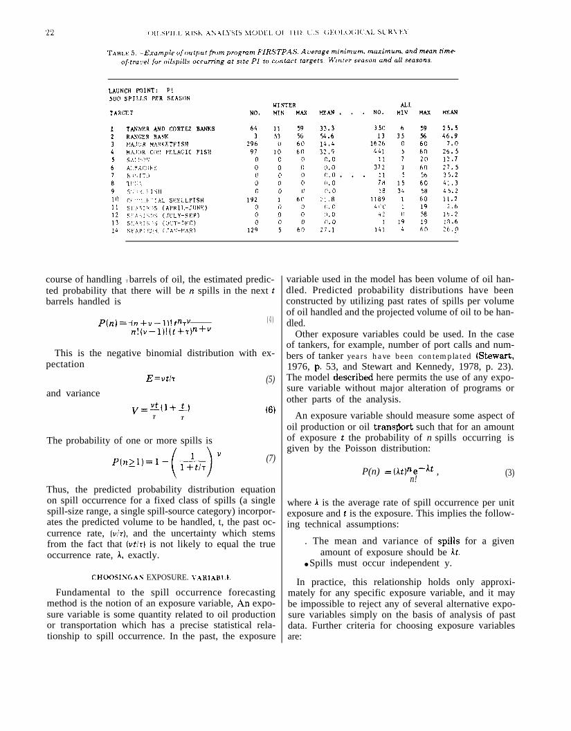
PROGR.4\1 FIRSTP.AS

Program FIRSTPAS calculates the a\,erage, mini-mum and maximum times-of-travel for oilspills occur-

ring at a given launch point to make first contact witha target. This tabulation, an example of which is shownin table 5, is presented by season as well as for the en-tire year. Spills which do not contact a target are notincluded in the statistics for that target.

Program FI RSTPAS was, in earlier versions of themodel, the only means of accounting for oilspill age.t$’hen H ITPROB was revised to present its results forspills of different travel times, FI RSTPAS becamepartially obsolete. However, it has still proven to be auseful program for checking the behavior of the modeland for helping to understand oilspill transport.

SPILL OCCURRENCE

This section describes how spill occurrence probabili-ties are estimated.

To construct the estimated probability distributionon spill occurrence for a fixed class of spills, certainsimplifying assumptions must be used which may beunsatisfactory in particular instances. The forecastingmethod used in the model is sufficiently flexible for in-corporation of new and specific assumptions, however,

The following were considered some desirable fea-t ures of a spill occurrence forecasting method:

1. The method should include an estimate of theuncertainty in the forecast by providing aprobability distribution rather than a pre-dicted number of spills.

2. The method should be consistent with past ob-servations and intuitively reasonable.

3. The dependence on past occurrence ratesshould be clear and explicit.

4. The method should be flexible; that is, changesin the assumptions concerning use of past oc-currence rates should be easily accommo-dated, and the method should be easy to up-date as new data are accumulated.

SOME B.4SIC FEATURES OF SPILL

O C C U R R E N C E F O R E C A S T I N G

Forecasts of oilspill occurrence are made via a pre-dicted probability distribution on the number of spillswhich might occur during the production life of a leasearea. The predicted distributions are constructed u s i n g13ayesian methods to incorporate the uncertainty dueto limited historic spill-incidence data. The appendixdescribes this method in detail.

Simple summary statistics to describe the frequencyof spills expected to occur during the production life ofa lease area must. be chosen to reflect, as best as pos-sible, the shape of the probability distribution. Consid-erable uncertainty in forecasting for a new offshorelease area is reflected in a predicted probability distri-

RISK (:.AL(:L’L.ATION

FICLRE 10.–Example oilspill trajectories for a spill site near southern California {OCS Lease Sale 48). Rectanglesare proposed lease tracts. Number on trajectory isLanfear. 1978).

bution with high variance, implying that one cannot ‘forecast a single number of future spills with muchconfidence. Presenting the “’expected number” of spillcan be misleading, as a wide range of possible spilltotals may be as likely to occur over the life of the leasearea as the “expected number, ” which is thehypothetical average over many lease area lifetimes.Thus, model forecasts are presented in terms of themost likely number of spills based on the predictedprobability distribution (in statistical terms, the mode

the time to the end point in days (Slack. Wyant, and

rather than the mean) as well as the predicted probabil-ity that one or more spills of a given size will occur inthe lifetime of a lease area.

Spill occurrence forecasts are made separately fordifferent spill-size categories. OilspiIIs of differentmagnitudes have different damage potentials, andmay be expected to exhibit different statistical proper-ties in their occurrence. The largest spills occur rela-tively rarely, but account for a large proportion of thetotal volume spilled. For example, the Argo Merchant

20 (J1l.SPll.L. RISK +S’+[.}”S[S il(_)l>E[. (JF 7-}{E U S (; EO1.(X,l CA[, SVR~’E~

TABLE 3.–Example of tvpical ou tput from program HITPROB, shouing pmbabitities (expressedin percent chancej that an oilspill starting at a particular locati”on usiil reach a certain ~rget in30 days

1., less than 0.5 percent chance ● , greater than 995 percent chance)

spilled 7.7 million gallons when it broke up off Nan.tucket in December 1976 (Grose and Mattson, eds.,1977, p. 1); by comparison, the total volume spilled in1975 by U.S. tankers was 7.8 million gallons in 587 in.cidents (Stewart, 1976, p. 60). The largest spills havethe most damage potential, and generally occur underdifferent circumstances from smaller spills. Majorblowouts of wells or complete ship breakups, for in-stance, are somewhat distinct from minor collisions orequipment malfunctions.

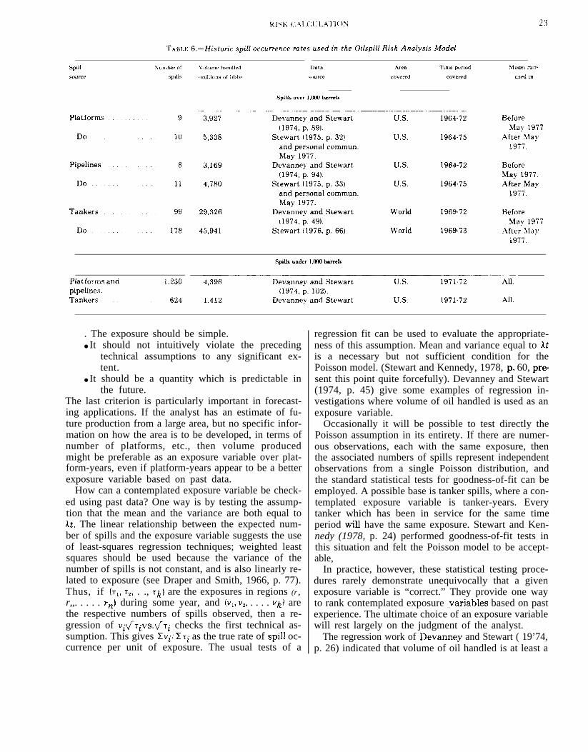
Spill occurrence forecasts are made separately fordifferent types of spill sources–tankers, pipeLines, andplatforms. It is reasonable to expect that spill occur-rence rates will differ for the various modes of produc-tion and transport, and past data support this conten-tion (see table 6). A principal use of the risk analysismodel has been to help compare transportation mech-anisms for given lease areas.

Continued accumulation of data may enable greaterrefinement of spill-source categorization in the future.

For example, tankers might be considered separatelyby age class (Stewart and Kennedy, 1978, p. 25), ordeep-water production rigs with single-buoy mooringsmight be considered separately from rigid, near-shorestructures. The exact approach taken for a given riskanalysis should depend on available data, the preciseconcerns of the analysis, and how the model results areto be interpreted; the model can be straightforwardlyapplied, using the same methodology, programs, andreporting structures as for the present pipeline-tankerbreakdown.

Spill occurrence forecasts, as well as any assessmentof risk from a given development program, depend fun-damentally on the estimated amount of oil to be pro-duced in a lwise area. First described by Devanney andStewart (1974), the Bayesian methodology used to con-struct the probability distributions on spill occurrenceutilizes past production and oilspill occurrence dataand future production estimates in a straight-forwardway. The following sections provide further details.

PREDICTED PROBABILITY DISTRIBL’TIOX FOR.4 FIXED CL.4SS OF SPILLS

This subsection describes the predicted probabilitydistribution for spill occurrence within a fixed class ofspills. A fixed class of spills consists of spills in a singles~e range (say, spills larger than a thousand barrels)originating from a single spill source (say, tankers).

A basic assumption of the method is that spills occuras a Poisson process, with volume of oil produced orhandled as the exposure variable. (Other exposure vari-ables can also be considered, as discussed in the nextsubsection. ) That is, the probability P, of observing nspills in the course of handling t barrels of oil is

13)

where A is the spill occurrence rate per unit exposure,(spills per million barrels of oil).

The Poisson assumption requires that spills occur in-dependently of each other. One could clearly questionthis assumption — if, for example, safety and inspec-tion standards were improved as a result of a particu-lar spill, several potentially subsequent spills might beaverted. hTonetheless, there is evidence that a Poissonmodel for spill occurrence provides a reasonable ap-proximation (see Stewart and Kennedy, 1978, p. 36}.

The spill occurrence rate, L is unknown. A Bayesianmethodology, described in detail in appendix A, pro-vides one way to w-eight the different possible values ofk, given the past frequency of spill occurrence for afixed class of spills by taking a weighted average of thedistributions (equation 3) over different values ofl. If uis the number of past spills in the fixed spill class in the

course of handling T barrels of oil, the estimated predic-ted probability that there will be n spills in the next tbarrels handled is

P(?z)= (~+v–l)!~nTvn!(~–l)!(t+T)n+v

(4)

This is the negative binomial distribution with ex-pectation

E=vth (5)

and variance

~=u(l+l) (6)T T

The probability of one or more spills is

(7)

Thus, the predicted probability distribution equationon spill occurrence for a fixed class of spills (a singlespill-size range, a single spill-source category) incorpor-ates the predicted volume to be handled, t, the past oc-currence rate, (v/T), and the uncertainty which stemsfrom the fact that (vt/T) is not likely to equal the trueoccurrence rate, L exactly.

CHOOSIXG AX EXPOSURE. V.+ RIABLE

Fundamental to the spill occurrence forecastingmethod is the notion of an exposure variable, An expo-sure variable is some quantity related to oil productionor transportation which has a precise statistical rela-tionship to spill occurrence. In the past, the exposure

variable used in the model has been volume of oil han-dled. Predicted probability distributions have beenconstructed by utilizing past rates of spills per volumeof oil handled and the projected volume of oil to be han-dled.

Other exposure variables could be used. In the caseof tankers, for example, number of port calls and num-bers of tanker years have been contemplated (Stewart,1976, p, 53, and Stewart and Kennedy, 1978, p. 23).The model describd here permits the use of any expo-sure variable without major alteration of programs orother parts of the analysis.

An exposure variable should measure some aspect ofoil production or oil trans@rt such that for an amountof exposure t the probability of n spills occurring isgiven by the Poisson distribution:

P(n) = (At)ne–At ,n!

(3)

where A is the average rate of spill occurrence per unitexposure and t is the exposure. This implies the follow-ing technical assumptions:

. The mean and variance of spi.lk for a givenamount of exposure should be it.

● Spills must occur independent y.

In practice, this relationship holds only approxi-mately for any specific exposure variable, and it maybe impossible to reject any of several alternative expo-sure variables simply on the basis of analysis of pastdata. Further criteria for choosing exposure variablesare:

. The exposure should be simple.● It should not intuitively violate the preceding

technical assumptions to any significant ex-tent.

● It should be a quantity which is predictable inthe future.

The last criterion is particularly important in forecast-ing applications. If the analyst has an estimate of fu-ture production from a large area, but no specific infor-mation on how the area is to be developed, in terms ofnumber of platforms, etc., then volume producedmight be preferable as an exposure variable over plat-form-years, even if platform-years appear to be a betterexposure variable based on past data.

How can a contemplated exposure variable be check-ed using past data? One way is by testing the assump-tion that the mean and the variance are both equal toAt. The linear relationship between the expected num-ber of spills and the exposure variable suggests the useof least-squares regression techniques; weighted leastsquares should be used because the variance of thenumber of spills is not constant, and is also linearly re-lated to exposure (see Draper and Smith, 1966, p. 77).Thus, if (1,, T,, . ., T~) are the exposures in regions (rl,r,,. . . . . rn) during some year, and (v,, v,. . . . . vh) arethe respective numbers of spills observed, then a re-gression of Vi~rTiVS. (Ti checks the first technical as-sumption. This gives Z~i/ X Ti as the true rate of spill oc-currence per unit of exposure. The usual tests of a

regression fit can be used to evaluate the appropriate-ness of this assumption. Mean and variance equal to Mis a necessary but not sufficient condition for thePoisson model. (Stewart and Kennedy, 1978, p, 60, present this point quite forcefully). Devanney and Stewart(1974, p. 45) give some examples of regression in-vestigations where volume of oil handled is used as anexposure variable.

Occasionally it will be possible to test directly thePoisson assumption in its entirety. If there are numer-ous observations, each with the same exposure, thenthe associated numbers of spills represent independentobservations from a single Poisson distribution, andthe standard statistical tests for goodness-of-fit can beemployed. A possible base is tanker spills, where a con-templated exposure variable is tanker-years. Everytanker which has been in service for the same timeperiod wilI have the same exposure. Stewart and Ken-nedy (1978, p. 24) performed goodness-of-fit tests inthis situation and felt the Poisson model to be accept-able,

In practice, however, these statistical testing proce-dures rarely demonstrate unequivocally that a givenexposure variable is “correct.” They provide one wayto rank contemplated exposure ,variables based on pastexperience. The ultimate choice of an exposure variablewill rest largely on the judgment of the analyst.

The regression work of Devanney and Stewart ( 19’74,p. 26) indicated that volume of oil handled is at least a

24 ()[LsPII.L RIsK .AY.+1.}’SIS iloi)E1. OF T-HE L.S (; EOL()(; I(:.AL SLRI’L}’

reasonable exposure variable. The variable is simple,bears a good intuitive connection to the number ofspills, and is relatively easy to predict in advance with-in known error limits. Recently, though, Stewart andKennedy (1978) have investigated the use of other ex-posure variables.

SPILL OCCL-RRENCE RATES AXD EXPOSURE V.$RI.4BLES

The sources for the spill occurrence rates used in themodel are Devanney and Stewart (1974), and Stewart(1975 and 1976). Those authors obtained data primari-ly from three sources: the Conservation Division of theU.S. Geological Survey, the U.S. Coast Guard, and asurvey of world-wide major tanker spills in 1969-1972(Devanney and Stewart, 1974, p. 1). In the past, therehave been many problems in screening and reconcilingthe information in these data sources; Stewart andDevanney have done much in this area and describe itin the above-cited reports. Table 6 gives the spill occur-rence information used to date in runs of the model.The occurrence rates were used to construct predictedprobability distributions on spill occurrence as des-cribed in the earlier subsection, “Predicted ProbabilityDistribution for a Fixed Class of Spills. ” For smallspills, pipelines and platform occurrences are lumpedtogether due to the data base ambiguity concerningthe precise division point between a platform and apipeline spill.

TRANSPORTATION SCENARIOS

The previous section presented a method for con-structing a probability distribution on spill occurrence.The next logical step is to show how site-specific de-tails are applied to calculations of spill occurrence.

COXSTRUCTION’ OF TR.4NSPORTATION SCEX.\RIOS:PROGR.4M SCEN.$R1O

The risks of oilspills resulting from OCS develop-ment do not arise solely from platform operations.Transporting oil to shore entails additional risks whichcan exceed the risks of extracting the oil. Therefore,each group of leasing tracts must be considered as partof an integrated production and transportation sys-tem; program SCENARIO provides a means of des-cribing this system so that spill occurrence probabilitydistributions can be calculated.

For each production site, a transportation routemust be defined by linking together any of the launchpoints analyzed by program SPILL with destinationpoints (see figure 11), The method of transport (that is,pipeline or tanker) must be specified for each transpor-tation route segment. It is not necessary for the routeto be strictly continuous, since this description is only

an approximation of an actual route. The modeler mustuse judgment in striking a balance between a preciseroute description and a reasonable computational ef-fort, and should be watchful against specifying a trans-portation route more detailed than justified by theresolution of the model. Figure 11 shows how oil produced from lease tract group P14 would be brought toland in tankers following a route starting at P14 andcontinuing through T21 and T20. At least onetransportation route must be defined for every leasetract group contained in an analysis, and the completeset of transportation routes is called the transporta-tion scenario. The coding of program SCENARIOallows the inclusion of sources of oilspill risk otherthan OCS leasing in a transportation scenario.

In the preceding subsection, “Spill Occurrence Ratesand Exposure Variables, ‘‘ it was explained that the ex-posure variable for transporting oil is the volume of oilhandled. That is, a given volume of oil, t, moved fromA to )3 can be expected to result in 1 t spills, regardlessof the distance between A and B. The route from A toB can be described as a series of launch points with theoilspill risks distributed among the route segments ac-cording to their length. (In figure 11, for example,typical weights may be 20 percent for P14, 40 percentfor T19, and 40 percent for T20, demonstrating a roughproportioning of risk to length.) Use of other exposurevariables would require a similar weighting of trans-portation route segments. To accomplish this, pro-gram SCENARIO is designed with a highly flexibleweighting process that allows the user to assign an ar-bitrary weight to each segment of a transportationroute. This flexibility allows the user to specify a com-plicated transportation route that involves multiplemovements of oil (e.g. “pipeline to port A, then tankerfrom port A to port B‘ ‘), or to divide the oil from a leasetract among several different transportation routes(that is, “half to port A, half to port B“). If deemed jus-tifiable, “high risk” transportation segments can evenbe assigned higher weights.

ESTI.~ATED VOLLl~ES OF OIL RESERVES

For calculating actual oilspill risks, it is necessary toinclude the volume of oil that is expected to be pro-duced from each lease tract group as input to programSCENARIO. This information is compiled by the Con-servation Division of the U.S. Geological Survey and isconsidered proprietary information.

PROBABILITY THAT AN OILSPILL WILLOCCUR AND CONTACT A TARGET

The model produces as an end result an estimatedprobability distribution for the number of spills con-

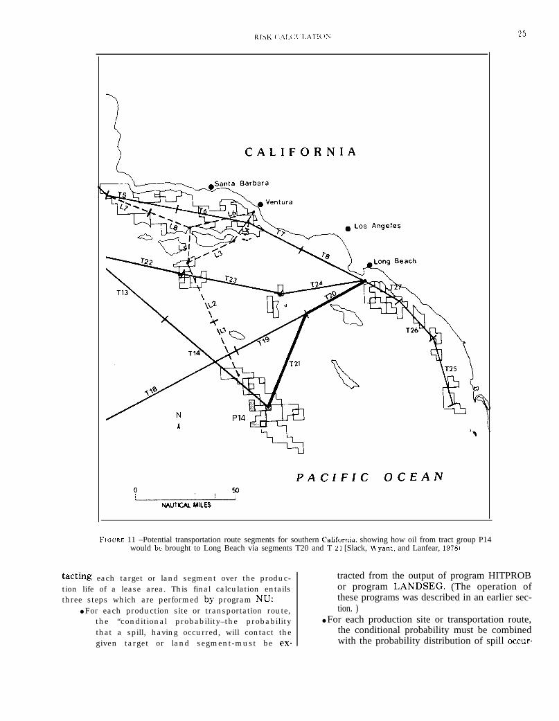
FIGURE 11 –Potential transportation route segments for southern Cahfornia, showing how oil from tract group P14would be brought to Long Beach via segments T20 and T 21 [Slack, Wyant. and Lanfear, 1978).

tacting each target or land segment over the produc-tion life of a lease area. This final calculation entailsthree steps which are performed by- program NW:

● For each production site or transportation route,the “conditional probability–the probabilitythat a spill, having occurred, will contact thegiven target or land segment-must be ex-

,,..3

tracted from the output of program HITPROBor program LANDSEG. (The operation ofthese programs was described in an earlier sec-tion. )

● For each production site or transportation route,the conditional probability must be combinedwith the probability distribution of spill occur-

2b 011. SP1l. I. R1\K ,\ NiI.}’s[s \lo L)EI. OF” ‘I-HE L“ s (; E()[.()GI(:.%1. sLR\”r.}

rence (estimated using the methods describedin the section “Spill Occurrence”) to yield asingle-source probability distribution for thenumber of hits on the target or land segment.This distribution may be arrived at by one oftwo methods, according to whether the singlesource is a “point” source, such as a produc-tion platform, or a “distributed’” source, suchas a tanker route where the oil could be re-leased anywhere along the route.

s All single-source estimated probability distribu-tions in a scenario (see the previous section)must be combined to yield the overall esti-mated probability distribution for the numberof hits on each target and(or) land segment.

The following subsections describe, in more detail, themethods employed,

PROB~BILIT1’ OF HITS OX .4 TARGETFROM A SINGLE SOURCE

Programs HITPROB, LANDSEG, SCENARIO,and NU communicate through files stored on perma-nently mounted disk packs. After obtaining the condi-tional probabilities for all targets and land segmentsfor each launch point, program NU begins to processthe transportation scenario, segment by segment.

Suppose that for production platforms, the esti-mated probability distribution of N’, the number ofspills occurring, is negative binomial. Then, followingfrom the section “Spill Occurrence, ”

P(N’–n) =(n+v–l)!t~U (4)n!(~—l)!(t+T)n+v

Suppose, further, that the conditional probability (ob-tained from HITPROB or LANDSEG) that a spillfrom a point source will hit a given target is p. Then,the estimated probability distribution of N’, thenumber of spills which both occur and hit the targetover exposure t, is negative binomial

P(N’=n)= (n +~ – l)!(pt)nTv (8)—.— -,

with mean

and var iance

o ’ =

Appendix A conta insSuit.

TZ!(U-l)!(@+T)n+v

i =VPt~T (9)

()V p t l+pt.— — . (10)~ ?\ /’

a rigorous derivation of this re-

For a distributed source defined by several transpor-tation route segments, suppose that the estimatedprobability distribution of spills is the negative bino-mial with parame~rs as before: v, the number of pastobserved tanker spills, T, the amount of past exposureobserved, and t, the predicted future exposure. Thesespills could occur at any point along the route. As theprevious sections pointed out, it is often desirable in arisk analysis to be able to weight points along a routein terms of that likelihood of spill occurrence. The con-straint on the weights is that the distribution of the to-tal number of spills along the route must be the above-mentioned negative binomial distribution, with mean

A= Vt/T (11)

and variance

( )~2=x 1+1 . (12)

T T

This constraint is satisfied by assuming that the distri-bution of spills at each transportation route segment isnegative binomial with parameters vi, Ti, an d ti, wherethe sum of the vi must be v. Appendix A demonstratesthat this structure satisfies the constraint.

To determine the estimated probability distributionfor hits on a target from spills along the whole route,the model first constructs the hit distribution for eachseparate point source along the route (using the pre-viously described methods for single point sources).The model then combines these distributions as des-cribed in the next section.

PROB.4BILITY OF HITS ON A TARGETFRO.M ?WCLTIPLE SPILL SOURCES

The overall estimated probability distribution forthe number of hits on a target is constructed as theconvolution of the appropriate single-source distribu-tions derived in previous steps. The meaning of thisstatement is best conveyed through an example: LetPI ,n be the probability of R spills hitting the targetfrom the first source, and P2,n be the probability of nspills hitting the target from a second source,

p =(~ +~i– l)!(Jl~ti)~Tivii, n

(13)n![Vi–l)!(pi~i+T~)n+vi

Let Pn represent the probability that n spills hit thetarget from both sources combined. Then,

P. =P, .P,,Q , (14)

P, = Pi ,P2,j+P:,oP2,,, (15)

\lo I)E1. \ FRIEl(:.\”I’i( )S 4S1) l. I\l[”I’.$”l’lo XS 27

P2 = P,,, P,,o + P,,, P,,, + P, ,P2,2, (16)

and,

Pn = i ~ ~ Pl,iP2(n–i) . (17)

The extension to more than two sources is similar.

Program NU carries out these calculations in themodel. Its design is such that the effects on a risk anal-ysis of different assumptions concerning incidencerates, production and transportation scenarios, or re-source estimates, can be determined simply andstraightforwardly by rerunning the program with dif-ferent parameter values.

M O D E L V E R I F I C A T I O NAND LIMITATIONS

FORhLAL ERROR ANALYSIS

Results of complex systems models are seldomamenable to formal error analysis, that is, to the ex-pression of error in the end result as a function of er-rors in input quantities. Often, the error as an inputquantity will be unobtainable or unquantifiable, or theerror’s effect on the overall analysis will be too ambi-guous. Furthermore, it is especially difficult to attacha single number representing “standard error” to theresults of a model run, when the results consist of a setof predicted probability distributions. In fact, the Bay-esian methods used in constructing the distributionsdescribed here explicitly incorporate some elements ofuncertainty (notably those in estimating spill inci-dence rate) and were developed, in part, for situationswhere classical error analysis seemed unsatisfactory.

This does not imply Lhat a useful assessment of mo-del reliability cannot be made, or that the results arecategorically unreliable. Three modes of testing areavailable to the model user: ( 1 ) an informal assessmentof individual model components is often satisfactory:(2) the sensitivity of the model results to particular as-sumptions can be tested by repeated runs with differ-ing inputs; and (3) parts of the model can be directlytested by comparison with actual spill trajectories.The following sections contain discussions of howthese modes of ei’aluation were applied to the modeldescribed here.

INFOR}fAL ERROR ANALYSIS

Several factors constrain the effective breadth of am o d e l ’ s a p p l i c a b i l i t y , T h e models s t ructure [how it

works, what it includes or excludes), the refinement of:he driving data, and the analytical treatment of thecomponent oilspill occurrence and movement pro-:esses all play a role. In a general purpose model, theselimitations will differ for each application of the model.This requires that the assumptions necessary for speci-fic areas be readily testable; different factors may limitthe precision of the results from case to case. As an ex-ample, unreliable current data may not seriously affectmodel output in situations where the movement of oilis largely wind-dominated (as in some proposed NorthAtlantic oil production areas–see Smith and others,1976b), but may critically affect model output wherecurrents are the primary mover (as in many proposedGulf of Mexico oil production areas–see Wyan~ andSlack, 1978), The computer programs of the modelhave been built to facilitate case-specific testing. Thishas been done by modularizing computer programs, byconcentrating on simple parameterizations of pro-cesses, and by restricting analytical representations ofphysical processes to those which are relatively simple,general, and widely accepted.

SP.ATI.4L RESOLUTION

The model cannot represent the locations of oilspillsor targets with any finer resolution than the cell size(about 1 nautical mile square) of the grid system. Thisis an artificial restriction, of course, in the sense thatthe model could be simply modified to diminish the cellsize. Increasing the spatial resolution of the model bythis means would, however, lead to a spurious and mis-leading impression of accuracy in the output, given thepresent accuracy with which the location of many tar-gets and the spreading of large spills can be depicted.

RISK FOR NE.+ R-SHORE.4XD CONFINED-ARE.{ SPILL SOURCES

The spill transport equation used in the model hasseveral virtues. It is simple, is widely accepted as a rea-sonable representation of oilspill movement in openwater (Stolzenbach and others, 1977, p. 5-47), and isvoid of any special assumptions which would disqual-ify the model for risk forecasting in most proposed off-shore production areas. However, due to the fact thatthe basic oil transport equation is designed to repre-sent the “average” movement of large spills in fairlyopen waters, the model cannot adequately representthe detailed movement of spills close to shore or in con-fined estuaries or bays, where tides and highly local-ized currents may dominate the movement of spilledoil.

SPRE.iDIXG

The model does not explicitly incorporate spreading.This deficiency is mitigated by several factors. First,because of the large regions over which the model is de-signed to operate and the resulting scale of model reso-lution, spreading is less important than overall advec-tion in determining risks. Second, the original digitiza-tion of targets and their insertion into the grid systemtends to expand the areas occupied by targets (any cellpartialIy occupied is treated as fully o c c u p i e d ) , a n dcauses “near misses” of oilspills to be counted as hits.T h i r d , r e c o r d i n g t h e t i m e - o f - c o n t a c t f o r e a c h h i tenables the analyst to estimate spreading effects inde-pendently, given information on oil type, sea state, andso on.

DEC.*Y

The modeling of spill decay presents the same diffi-culties as the modeling of spreading, in that knowledgeof factors such as oil type are integral to analytical des-criptions of the physical process. As with spreading,the model does not explicitly calculate decay, but isconstructed to provide information on spill travel time,thus enabling assessment of the extent to which decaymight mitigate predicted impacts, Contacts of spillswith targets are compiled in several elapsed-time cate-gories–up to 3 days, 3 to 10 days, 10 to 30 days, and30 to 60 days–to assist the analyst in this assessment.

SENSITIVITY ANALYSIS

Sensitivity analysis of model assumptions is a usefultechnique for assessing model strengths and weak-nesses. As suggested above, such analyses should betailored to particular situations: different features ofthe model are critical in different situations, and thedictates of economy require the appropriate selectionfrom the many possible sensitivity analyses. Designfeatures of the model make such analyses easy to carryout.

Two sensitivity analyses performed during a risk an-alysis for proposed North Atlantic OCS productionareas (Smith and other, 1976 b), exemplify the kinds ofanalyses which can be readily performed. The basictransport equation includes the wind drift angle, whichis the number of degrees wind-induced oil movementsare deflected from the direction of the wind by Coriolisacceleration. Some contro\’ersy surrounds the optimalvalue of this parameter for spill modeling, but mostsuggested values fall between O and 20 degrees clock-wise in the Northern Hemisphere (Stolzenbach andothers, 1977, p. 81). For the ?iorth Atlantic risk analy -

sis, two separate model runs were made using driftangles of O and 20 degrees clockwise. The resulting es-timates of probabilities of spills from the proposed oilproduction areas hitting shore were 21 and 8 percent,respectively.

In another sensitivity analysis for the same area, ac-tual historic wind sequences were substituted for sto-chastically generated ones (see the section on“Winds’ ‘). Table 7 shows the estimated probability ofhitting land for spills from one proposed North Atlan-tic oil production site by the two modes of model opera-tion.

These two studies convey the kinds of evaluationswhich can be conducted in the course of a risk analysis,and the sensitivity of results to certain key assump-tions. Different sensitivities to these particular as-sumptions can be obtained in different OCS areas.

DIRECT 310DEL VERIFIC.4TION

Clearly, predictions of expected numbers or probabil-ities of spill impacts for a given place and time cannotbe “proved” or “disproved” by a single spill. Nonethe-less, a limited verification of the trajectory model wasachieved for the area covered by the North AtlanticOCS oilspill risk analysis (Smith and others, 1976b). InDecember 1976 the Argo Merchant spilled 7.7 milliongallons of oil and the spill traveled in the direction thatthe model indicated was most likely (see fig. 12). Ex-tensive overflights and monitoring of this spill provialed data for a more thorough evaluation of compo-nents of the model, In particular, by comparing actualand simulated spill locations, the validity of current as-sumptions, transport equations, and wind data sourcechoices could be examined. This work, presented in de-tail in Grose and Mattson (1977), Pollack and Stolzen-bach (1978), and Wyant and Smith (1978), supportedthe general adequacy of the transport segment of themodel.

The spill occurred not as an idealized instantaneouspoint spill but rather was released over an extendedperiod of time. To facilitate comparisons of simulatedtrajectories with the actual spill, the spill was modeledas a set of sequentially released points, with each3-hourly wind applied to the entire, gradually enlarg-ing set. This enabled 2-dimensional construction ofspill representations such as that in figure 12. Runswere made using a variety of different parametervalues. Graphical output such as that in figure 12seems to be a particularly appropriate way to commun-icate the validity of risk forecasts to potential modelusers in that it quickly and concisely gives a feeling forthe model’s level of approximation.

\lo I)l.l< OL” I’I’L” I ,\\l) (’\sF: I: X,4 X1l’[, ES 1(]-.

TABLE 7,–Sensih’uify of predicted oilspills n“sks for the NorthAtlantic study area to the assumption that uinds can bemodeled as a first-order Markoc process.

Wmd sequence

.-Generated

from firstorderMarkovprocess.

Takendirectlyfromhistoricrecord.

\wnb+r of

shmulawd

wa]wmrtes

pm season Percent OF ~mndated trajectories hltt]ng shore

IYmter Spring Summer Fall Total

.500 1 8 19 3 8

300 0 12 8 0 5

MODEL OUTPUT AND CASE EXA,MPLES

REPORTS FOR OCS LEASING

For each application of the model to a Federal OCSlease sale, a final report is produced which includes thefollowing items:

● A discussion of the data sources whichwere used.

● Maps showing the location of the study areaand the locations of the targets and land segments.

● Tables of conditional probabilities giving, foreach launch point, the probabilities that an oil-spill Occurnng at a given production site willcontact targets or land segments within 3, 10,30, and 60 days.

● Tables and graphs showing the probabilities ofoilspills occurring.

● Tables showing the overall probabilities of oil-spills occurring and contacting targets or landsegments withid 3, 10, 30, and 60 days.

A list of reports prepared for seven previous analy-ses is presented in table 8.

S~%l}l.iRY OF RESULTS TO DATE

The model has been used to conduct oilspill risk anal-yses for eight OCS lease sales in six Federal leaseareas, which together represent only a small fraction ofthe total number of offshore tracts that may be devel-oped eventually. Nevertheless, the six areas studiedthus far are distributed among all four of the major

TA~LF- 8.–Reports prepared for OCS lease sale analyses using theOilspill Rwk Analysis Model of the U.S. Geological Surt,ey

An Oilspill Risk .4nalysis for the Southern California (Proposed SaleW) Outer Continental Shelf Lease Area: James R. Slack.Timothy Wyant, Kennth J. Lanfear; U.S. Geological SurveyWater-Resources Invest igat ions 78-80; 1978: 101 p.(Available from NTIS. )

An Oilspill Risk Analysis for the Mid-Atlantic ( Proposed Sale 49)Outer Continental Shelf Lease Area; James R, Slack andTimothy Wyant; U.S. Geological Survey Water-ResourcesInvestigation 78-56: 1978; 79 p. (Available from NTIS, )

An Oilspilf Risk Analysis for the Eastern Gulf of Mexico (ProposedSale 65) Outer Continental Shelf Lease Area; Timothy Wyantand James R. Slack. U.S. C,eological Survey Open-File Report78-132; 1978; 72 p.

.4n Oilspill Risk Analysis for the ~’estern Gulf of Alaska I KodiakIsland) Outer Continental Shelf Lease Area; James R. Slack,Richard A. Smith. and Timothy Wyant; U.S. GeologicalSurvey Open-File Report 77-212[ 1977; 57 p.

An Oilspilf Risk Analysis for the South Atlantic Outer ContinentalShelf Lease Area; James R. Slack and Richard A. Smith; U.S.Geological Survey Open-File Report 76-653; 1976:54 p.

An Oilspill Risk Analysis for the Mid. Atlantic Outer ContinentalShelf Lease Area; Richard A. Smith, James R. Slack, andRobert K. Davis: U.S. Geological Survey Open.File Report76-451: 1976a: 24 p.

.4n Oilspill Risk Analysis for the North Atlantic Outer ContinentalShelf Lease Area; Richard A. Smith, James R. Slack. andRobert K. Davis; U.S. Geological Survey Open-File Report76-620: 1976b; 25 p.

OCS regions which will experience oil and gas develop-ment (the Atlantic and Pacific coasts, the Gulf of Mex- ‘ice, and the Alaskan Peninsula) and will serve as focalpoints for further development in those regions.

The primary objective of oilspill risk analyses con-ducted by the Geological Survey is to determine therisks of petroleum development for the tracts within agiven lease area. Such information is useful to the Fed-eral Government in selecting tracts to offer for salefrom a list of tracts proposed for development by theoil industry. It is also of interest, however, to makecomparisons in oilspill risk between lease areas, sincethe sites represent the four major OCS regions and thepossibility of large differences in risk exists. An inter-regional comparison will be the emphasis of the sum-mary presented here. (For more detailed descriptionsof studies of individual lease areas, the reader is di-rected to the bibliography of oilspill risk reports intable 8.)

An important question concerning oilspill risk inFederal areas is whether there are significant geo-graphic differences in spill risk per unit of expected oilproduction. (Risk per unit production can be measuredas expected number of spill impacts on a given re-source or shoreline segment per billion barrels pro-

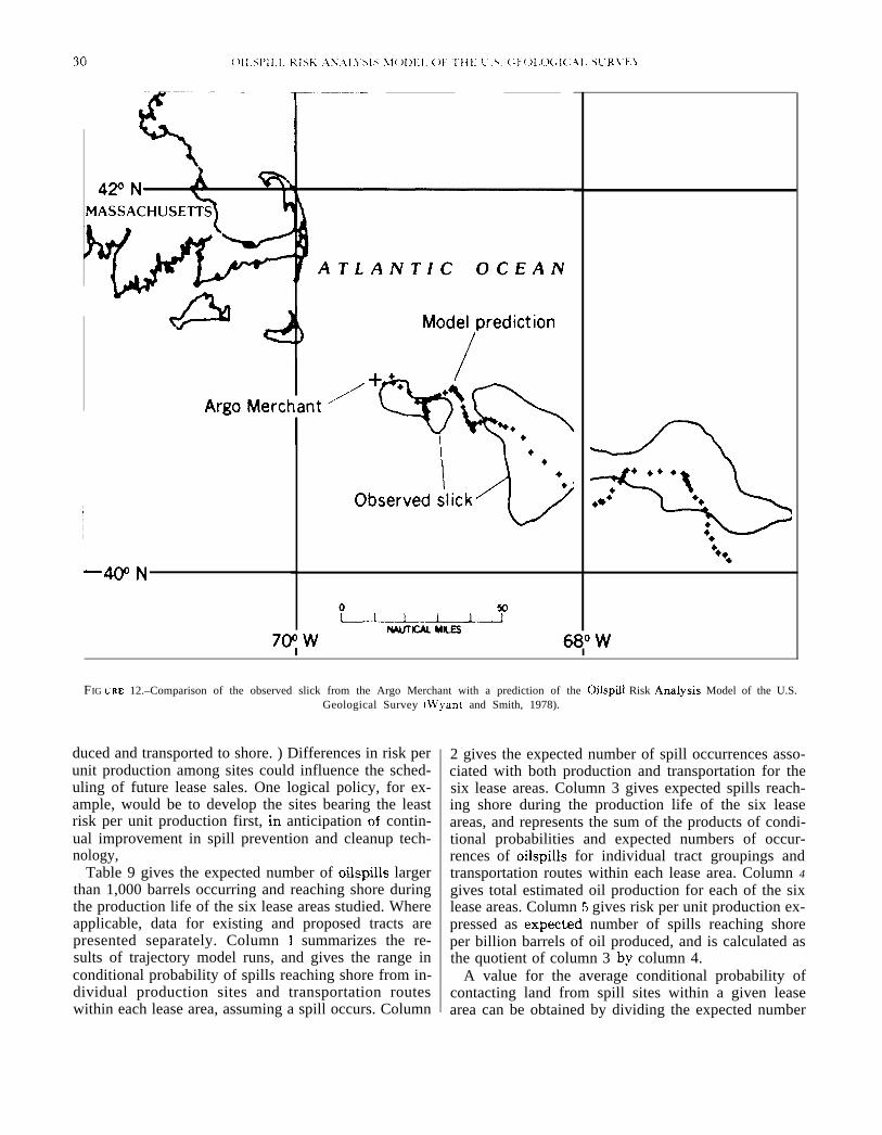
FIG CBE 12.–Comparison of the observed slick from the Argo Merchant with a prediction of the Oilspill Risk .4nalysis Model of the U.S.Geological Survey (Wyant and Smith, 1978).

duced and transported to shore. ) Differences in risk perunit production among sites could influence the sched-uling of future lease sales. One logical policy, for ex-ample, would be to develop the sites bearing the leastrisk per unit production first, in anticipation of contin-ual improvement in spill prevention and cleanup tech-nology,

Table 9 gives the expected number of oilspills largerthan 1,000 barrels occurring and reaching shore duringthe production life of the six lease areas studied. Whereapplicable, data for existing and proposed tracts arepresented separately. Column I summarizes the re-sults of trajectory model runs, and gives the range inconditional probability of spills reaching shore from in-dividual production sites and transportation routeswithin each lease area, assuming a spill occurs. Column

2 gives the expected number of spill occurrences asso-ciated with both production and transportation for thesix lease areas. Column 3 gives expected spills reach-ing shore during the production life of the six leaseareas, and represents the sum of the products of condi-tional probabilities and expected numbers of occur-rences of oilspills for individual tract groupings andtransportation routes within each lease area. Column 4

gives total estimated oil production for each of the sixlease areas. Column 5 gives risk per unit production ex-pressed as expectid number of spills reaching shoreper billion barrels of oil produced, and is calculated asthe quotient of column 3 by column 4.

A value for the average conditional probability ofcontacting land from spill sites within a given leasearea can be obtained by dividing the expected number

of spills reaching shore (column 3) by the expectednumber of spills occurring (column 2).1 In the NorthAtlantic, for example, the average conditional proba-bility of a spill reaching shore, given that one has oc-curred on a randomly selected tract, is 46 percent(1.1 - 2.4). It can be seen from table 9, column 1, thateven within the same lease area, the probability of oil-spills reaching shore from different tracts and trans-portation routes is quite variable. Ranging from lessthan 20 percent to nearly 80 percent in a majority oflease areas, the spread in conditional probability re-flects variability in wind and current patterns withineach area as well as geographic differences, such as thedistance of potential spill sites from shore. The varia-tion in risk among different potential drilling sites andtransportation routes is, in itself, evidence of the needfor an effective methodology for estimating risk priorto tract selection.

More to the point of the present summary, however,are the large differences in oilspill risk between thelease areas, as seen in table 9. By far, the lowest risk ofspills reaching shore exists in the Mid-Atlantic area,where the total expected number of spills reachingshore over the production life of both existing and pro-posed leases is only 0.19, In all other areas, the expec-tation of spills reaching shore is at last 6 times higherthan in the Mid-Atlantic, and for southern California,the expectation is more than 50 times higher. A majorreason for low risk values in the Mid-Atlantic area isclear in the results of trajectory model runs for that

area (Smith and others, 1976; Slack and Wyant, 1978):the predominance of westerly winds and the great dis-tance of tracts from shore (50 to 100 miles) combine tomake the conditional probability of reaching shorecomparatively low (1 to 42 percent).

The most significant comparison of oilspill riskamong Federal OCS areas is given in the figures for ex-pected contacts with shoreline per unit production(table 9, column 5). It is worth noting that values forexpected impacts per unit production are nearly inde-pendent of estimated oil production since productionestimates appear both in the denominator and numera-tor of the calculation. Thus any errors in predicting oilproduction are not carried over into this measure of oil-spill risk.

In terms of risk per unit production, the greatestcontrast is, again, between the Mid-Atlantic lease area,where the expectation of spills occurring and reachingshore is less than one per billion barrels produced, andthe southern California lease area, where the expecta-tion is more than five landings per billion barrels pro-duced. Overall, three lease areas stand out as havingcomparatively high risks of onshore impacts per unitproduction. These are the southern California easternGulf of Mexico, and South Atlantic areas-each withrisk values greater than 2,5 landings per billion barrelsproduced. The Gulf of Alaska and the North Atlantictogether compose a sort of medium risk category, withlanding expectations of 2.3 and 2,2 per billion barrels,respectively.

All of the above statistics refer to the risk of oilspillsreaching the shoreline within the boundaries of the dig-ital map used to track spill trajectories. Since so manyresources vulnerable to spilled oil are located on or

32 O1[. SPII. L ,RISK .AN.A. [.}’SIS \lo I)].1. ( ‘“ . . . . . . . . . . . . . . . . . . . . . . . . . .

near the shoreline, probability of contacting land isperhaps the best single descriptor of the risk of oilspilldamages in OCS lease areas. However, the probabilityof contacting land is not always an indicator of theprobability of impact on all the resources, and it is ad-visable to avoid condensing the description of oilspillrisk into a single number. For this reason oilspill riskanalyses have considered risk to an extensive list ofspecific resources (typically 20-30) for each lease area.

Table 10 compares OCS Lease areas on the basis ofoilspill risk to six general categories of coastal and ma-rine resources. The second part shows the expectednumber of contacts with each resource category perbillion barrels produced. For the most part, the oilspillrisk values in table 10 follow the same pattern estab-lished in table 9; that is, the lowest impact probabili-ties appear for the Mid-Atlantic lease area, and thehighest appear for the southern California lease area.There are three important instances in table 10, however, where oilspill risk is not highest for the southernCalifornia area. These are high-density resort and rec-reation areas (highest for the South Atlantic), criticalwaterfowl and seabird habitat (highest for the Gulf ofAlaska), and marine mammal concentration areas (alsohighest for the Gulf of Alaska).

OTHER POSSIBLE USES OF THE MODEL

Although the primary purpose of the model is to as-sess oilspill risks from OCS lease sales, it has severalother potential applications. Wyant and Smith (1978)described how the model was used in a “real time”mode to predict movement of oil spilled from the tank-er Argo Merchant. A lease sale analysis had ordy re-cently been completed that included the area of thegrounding, and the necessary data files were already inexistence. Because subsequent model runs have ex-panded the model’s data base to include major por-tions of”the U.S. Outer Continental Shelf, operation inthe real time mode would be possible in many other sit-uations. Conversion to real time operation is relativelysimple: data files must be retrieved from tape archives,and program SPILL must be modified so that eachMonte Carlo trajectory run begins with a “present”wind velocity. However, it must be emphasized thatsuch use is an extension beyond the original model de-sign, and may not be as efficient nor as technicallysound as using models designed specifically for oilspillcleanup.

The model’s risk assessment capabilities are not li-mited to risks of OCS lease sales; other potentialsources of oilspills, such as tanker import routes, canbe analyzed as well. Since data files must be estab-lished for OCS lease sales in any case, the marginalcosts of including other oilspill risks are small.

PRACTICAL ASPECTS OF OPERATINGAND lMANAGING THE MODEL

The model has been used to analyze oilspill risks ineight OCS lease sales, and its continued use is antici-pated for future sales. To give potential users a realis-tic appraisal of the effort involved in model operation,this section discusses the practical aspects of operat-ing the model. The management system which hasevolved over three years of modeling operations is des-cribed, and the necessary software and hardware sup-port for the model is identified.

MANAGEhiENT SYSTEM

The model is constructed as a network of modules, ortasks. Each module is designed to accomplish a singlespecific objective using, as input, output produced byearlier modules. The major elements of a completemodel run are illustrated in figure 13.

Modular construction is not unusual for large mo-dels, as it greatly simplifies the modification process.The internal workings of any module may be freelychanged, as long as its input and output remain com-patible with associated modules.

The network shown in figure 13 can produce an OCSlease sale analysis–from data input to final report–infour months. Initial priorities are to establish a refinedset of input data files for program SPILL, and to iden-tify alternative leasing and transportation scenarios.As program SPILL requires a substantial amount ofcomputer time, every effort is made to find and correcterrors in the data submitted to SPILL before the latteris executed. Trajectory test runs help to spot data er-rors and to identify a sat@ factory set of launch pointsfor potential spills. Program SPILL produces nothingmore than a disk file containing the outcome of each.Monte Carlo trajectory run, which subsequent pro-grams use to generate conditional probabilities. Thelatter are combined with leasing and transportationscenarios to determine overall probabilities.

The different stages of model development for a typi-cal sale may produce as many as 50 files. All of theseare saved on disk, so that the analysis can be restartedat any intermediate point. Printouts associated withcreating these files serve a valuable function in qualitycontrol, and help to document the progress of a modelrun.

SOFTWARE

There are 21 computer programs used in the presentversion of the model, all written in IBM FORTRANIV, Level H. An extensive library of subroutines andfunctions (written in either assembly language or FOR-TRAN), in addition to the system libraries, is also em-

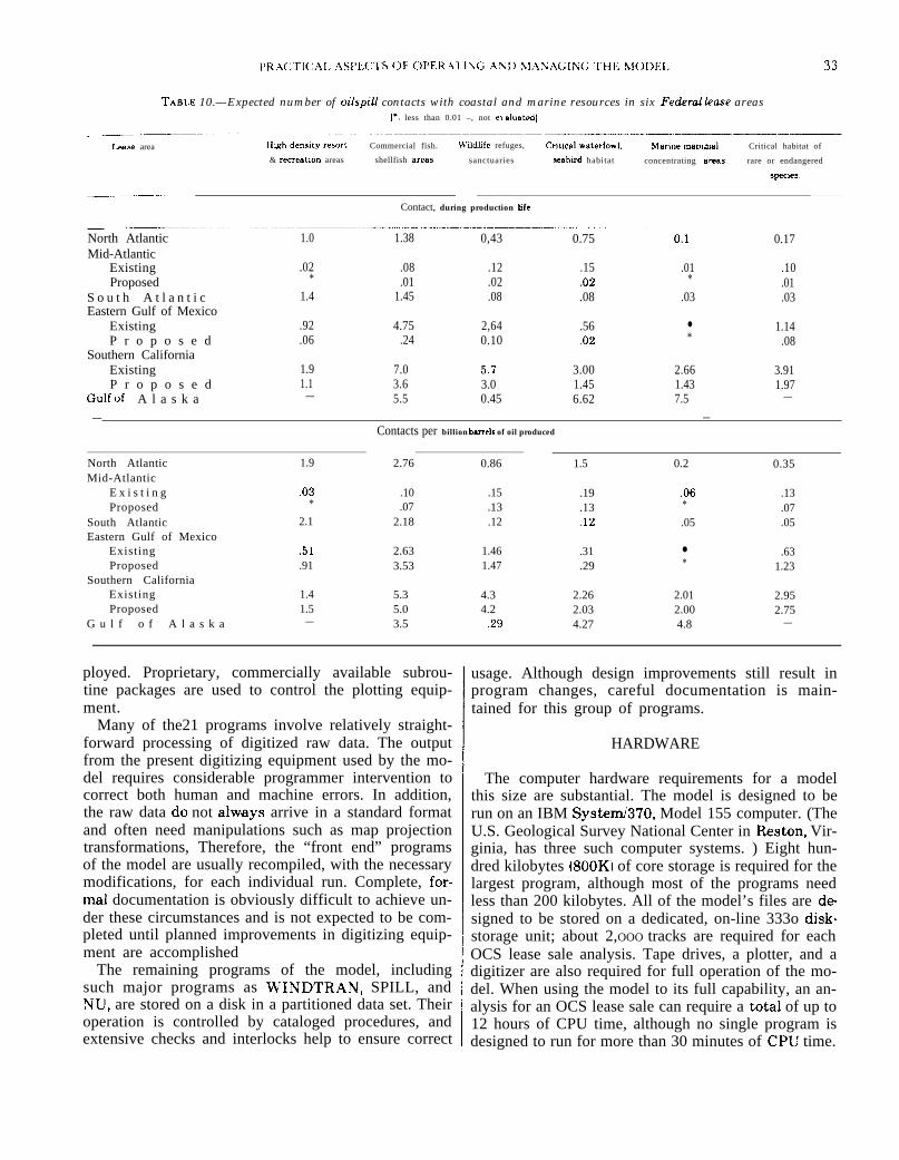
TABLE 10.—Expected number of oilspill contacts with coastal and marine resources in six Fedeml fease areas[“. less than 0.01 –, not e, AIF,w..3]

L.3se area High density resort Commercial fish. Wddfife refuges, CritIcaf wat.arfowl. .Marme mammnl Critical habitat of

& recreahon areas shellfish areas sanctuaries seabird habitat concentrating areas rare or endangered

Speclcls.

____— — ——

Contact, during production life

North Atlantic 1.0 1.38 0,43Mid-Atlantic

0.75 0.1 0.17

Existing .02 .08 .12 .15 .01Proposed

.10* .01 .02 .02 *

S o u t h A t l a n t i c.01

1.4 1.45 .08 .08 .03 .03Eastern Gulf of Mexico

Existing .92 4.75 2,64 .56 ●

P r o p o s e d1.14

.06 .24 0.10 ,02 * .08Southern California

Existing 1.9 7.0 5.7 3.00 2.66P r o p o s e d

3.911.1 3.6 3.0 1.45 1.43 1.97

Gulfof A l a s k a — 5.5 0.45 6.62 7.5 —

— —Contacts per billion barrele of oil produced

North Atlantic 1.9 2.76 0.86 1.5 0.2Mid-Atlantic

0.35

E x i s t i n g ,03 .10 .15 .19Proposed

.06 .13* .07 .13 .13 *

South Atlantic.07

2.1 2.18 .12 ,12 .05 .05Eastern Gulf of Mexico

Existing .51 2.63 1.46 .31 ●

Proposed.63

.91 3.53 1.47 .29 * 1.23Southern California

Existing 1.4 5.3 4.3 2.26 2.01 2.95Proposed 1.5 5.0 4.2 2.03 2.00 2.75

G u l f o f A l a s k a — 3.5 .29 4.27 4.8 —

ployed. Proprietary, commercially available subrou-tine packages are used to control the plotting equip-ment.

Many of the21 programs involve relatively straight-forward processing of digitized raw data. The outputfrom the present digitizing equipment used by the mo-del requires considerable programmer intervention tocorrect both human and machine errors. In addition,the raw data do not always arrive in a standard formatand often need manipulations such as map projectiontransformations, Therefore, the “front end” programsof the model are usually recompiled, with the necessarymodifications, for each individual run. Complete, for-mal documentation is obviously difficult to achieve un-der these circumstances and is not expected to be com-pleted until planned improvements in digitizing equip-ment are accomplished

The remaining programs of the model, includingsuch major programs as W’INDTRAN, SPILL, andN-U, are stored on a disk in a partitioned data set. Theiroperation is controlled by cataloged procedures, andextensive checks and interlocks help to ensure correct

usage. Although design improvements still result inprogram changes, careful documentation is main-tained for this group of programs.

HARDWARE

The computer hardware requirements for a modelthis size are substantial. The model is designed to berun on an IBM System1370, Model 155 computer. (TheU.S. Geological Survey National Center in Reston, Vir-ginia, has three such computer systems. ) Eight hun-dred kilobytes (800K) of core storage is required for thelargest program, although most of the programs needless than 200 kilobytes. All of the model’s files are designed to be stored on a dedicated, on-line 333o disk-storage unit; about 2,OOO tracks are required for eachOCS lease sale analysis. Tape drives, a plotter, and adigitizer are also required for full operation of the mo-del. When using the model to its full capability, an an-alysis for an OCS lease sale can require a total of up to12 hours of CPU time, although no single program isdesigned to run for more than 30 minutes of CPU time.

34

FIGURE 13.– Flow chart illustrating the major elements of a complete model run.

Programs requiring a longer time are broken into sev- placing a noticeable strain on computer center opera-eral jobs and the output files are concatenated. Some tions, and are usually scheduled for execution at off-programs, particularly program SPILL, are capable of peak hours.

sF.l, F,(: I“F,l) RF. FEREX(:ES 35

SELECTED REFERENCES

Allen, J., and Thanarajah, J. C. M., 1977, Laboratory studies of thevelocity of windon the movement of oil slicks: in Journal ofHydrauIic Research, v. 15, no. 4.

Blummer, M.. Sonza, S., and Sass, J., 1970, Hydro- carbon pollutionof edible sheUfishby an oil spill: Marine Biology Internation.al Journal on Life in Oceans and Coastal Waters, v. 5, no. 3, p.195-202.

Box, G. E. P., and Tiao, G. C., 1973, Bayesian inference in statisticalanalysis: Reading, Massachusetts, Addison-Wesley Publish-ing Company, 588 p.

Conrad, J. M., 1977, Oil spills: The policy of prevention and thestrategy of recovery: water Resources Research Center, Uni-versity of Massachusetts, Amherst, Publication No. 93.

Csanady. G. T., 1973, Turbulent diffusion in the environment: Bos-ton, D. Reidel Publishing Co., Geophysics and AstrophysicsMonographs, v. 3.

Danenberger, E. P.. 1976, Oil spills, 1971-75, Gulf of Niexico OuterContinental Shelf: U.S. Geological Survey Circular 741, 47 p.

Devanney, J. ~., III, and Stewart, R. J., 1974, Analysis of oilspillstatistics: Report to Council on Environmental Quality,Washington D. C., 126 p.

Draper. N. R.. and Smith, H., 1966, Applied regression analysis:New York, John Wiley, 407 p.

Feller, Wi~am, 1966, An introduction to probability theory and itsapphcations: New York, John Wiley, 461 p,

Grose, P. L., and Mattson, J. S. eds., 1977, The Argo MerchantOilspill; A Preliminary Scientific Report: NOA A

Jeffery, P. G.. 1973, Large-scale experiment on the spreading of oilat sea and its disappearance by natural forces, in Proceedingsof Conference on Prevention and Control of Oil Spills (1973):p. 469-474.

Kirwan, A. D., Jr., McNaHy, G., Pazan, S., and Jyert, R., 1979,Analysis of surface current response to wind: in Journal ofPhysical Oceanography, American Meteorological Society, V.9, no. 2.

Murray, S. P., Smith, W. G., and Shaw, C. J., 1970, Oceanographicobservations and theoretical analysis of oil slicks during the

Chevron spill, March 1970: Coastal Studies Institute, Louisi-ana State University, Baton Rouge, Louisiana, Technical Re-port no. 87.

Murty, T. S., and Khandekar, -M. L., 1973, Simulation of movementof oil slicks in the Strait of Georgia using simple atmosphericand ocean dynamics: in Proceedings of the 1973 Conferenceon the Prevention and Control of Oil Spills.

Nelson, W. L., 1958, Petroleum refinery engineering, New York,.McGraw-HiU.

Offshore Oil Task Group. 1973, The Georges Bank petroleum study,v. 11: Massachusetts Institute of Technolo~ Sea Grant Re-port, 311 p.

PhiUips, C, R., and Groseva V. N., 1977, The spreading of crudeoil spills across a lake: in Water, Air, and Soil Pollution, v. 8,no. 3, p. 353-360.

Pollack, A. Xl.. and StoLzenbach, K, D., 1978, Crisis science: investi-gations in response to the Argo Merchant oilspill: hlassachu-setts Institute of Tecttnolo~, Cambridge, }Iassachusetts.

Royer, T. R,, 1979, Personal communication to D. Amstutz, U.S.Bureau of Land Management, March 23, 1979.

Slack, J. R., and Smith, R. A., 1976, An oilspilf risk analysis for theSouth Atlantic Outer Continental Shelf lease area: U.S. Geo-logical Survey Open-File Report 76-653, 54 p.

Slack, J. R., Smith, R. A., and Wyant, Timothy, 1977, An oilspillrisk analysis for the Western Gulf of Alaska (Kodiak Island}Outer Continental Shelf lease area: US, Geological SurveyOpen-File Report 77-212.

Slack, J. R,, and W’yant, Timothy, 1978, An oilspill risk analysis forthe \lid.Atlantic (Proposed Sale 49) Outer Continental Shelflease area: U.S. Geological Survey Open-File Report 78-56.

Slack, J. R. Wyant, Timothy, and I.anfear, K. J,, 1978, An oilspillrisk analysis for the Southern California (Proposed Sale 48)Outer Continental Shelf lease area: U.S. Geological SurveyOpen-File Report 78-80,

Smith, J. E., cd., 1968, Torrey Canyon pollution and marine life:Cambridge Unit, ersity Press, Cambridge, United Kingdom.

Smith, R. A,, Slack, J. R., and Davis, R, K., 1976a, An oilspiU riskanalysis for the Mid-Atlantic Outer Continental Shelf leasearea: U.S. Geological Survey Open-File Report 76-451, 24 p.

Smith, R. .4., Slack, J. R,, and Davis, R. K., 19’76b, .4n oilspiU riskanalysis for the North Atlantic Outer Continental Shelf leasearea: U.S. Geological Survey Open-File Report 76-620, 50 p.

Stewart, R. J., 1975, Oil spiUage associated with the development ofoffshore petroleum resources, in Report to Organization forEconomic Co-operation and Development, 49 p.

Stewart, R. J., 1976, A survey and critical review of U.S. oil spilldata resources with application to the tanker pipeline contro-versy: Report to U.S. Department of the Interior, Washington D. C., 69 p.

Stewart, R. J., and Kennedy, M. B,, 1978, An analysis of U.S. tank-er and offshore petroleum production oil spiUage through1975: Report to Office of Policy Analysis, U.S. Department ofthe Interior, Contract Number 14-01-0001-2193.

Stolzenbach, K. D., Madsen, 0. S., Adams, E. E., PoUack, A. M., andCooper, C. K., 1977, A review and evaluation of basic tech-niques for predicting the behavior of surface oil slicks: RalphM. Parsons Laboratory, Report no. 222,

U.S. Department of the Interior, Bureau of Land Management,1977, Proposed 1977 Outer Continental Shelf oil and gaslease sale in the Western Gulf of Alaska: (OCS Draft Environ-mental Impact Statement), 4 volumes,

Wardley-Smith, J., cd., 1976, The control of oil pollution on the seaand inland waters, Graham and Trotman, Ltd., United Kingdom. 251 p.

W’yant, Timothy, and Slack, J. R.. 1978, An oilspiU risk analysis forthe Eastern Gulf of Mexico (Proposed Sale 65) Outer Contin-ental Shelf lease area: L1. S. Geological Survey OpenFife Report 78-132.

}$yant, Timothy, and Smith, R. .A., 197S, Risk forecasting for theArgo \lerchant spill: in Proceedings of a Symposium heldJanuary 11-13, 1978, at Khe Center for Ocean \lanagementStudies. L’niversity of Rhode Island. p. 2%.

Zilitinkevich, S. S., 1978, An evaluation of the oceanic surface driftcurrent speed and direction: in Boundary Layer Methodol-o~, v. l-i. no. 1.

APPENDIX

38 011.> P1[, I. R[SK AX. AI. }’SIS \I()[)EI, OF ‘I”}+F. I_’ s (; E()[LX;lC:,+l. S~R\” E}”

DISTRIBUTION THEORY OF SPILL INCIDENCE1. The derivation of the predicted probability distribu-tion

This appendix describes rigorously the derivation ofthe predicted probability distribution on spill occur-rence given as equation 4, in subsection “PredictedProbability y Distributions for a Fixed Class of Spills. ”The development is a Bayesian one; a good general de-scription of these Bayesian inference techniques maybe found in Box and Tiao, (1973, p. 1-73). The applica-tion of these methods to oilspill occurrence forecastingwas proposed and described in Devanney and Stewart,(1974).

We will use the following terminology:n = number of future spills,t = future exposure,i = true rate of spill occurrence per unit ex-

posure,u = number of spills observed in past,T = past exposure,

f(n) = a marginal probability density on n, andf(nl y) = the conditional probability density of n

given that the random variable y = y.

Assume that spills occur at random with some intensi-ty, p(n):

(A-1)

Suppose that, in the absence of information about A, wechoose to represent our uncertainty about thisparameter in the form of an “improper” prior densityon k

(A-2)

This says, in effect, that with no spills ever havingbeen observed, we place a good deal of faith on I beingequal to O, although we allow a priori the possibilitythat it may be any positive number. This may seem ar-tificial (as is often the case with Bayesian ignorancepriors), but note that in any case all it takes is one ob-servation of a spill to refute the notion that i = O. Ourprevious feelings in the absence of any data will beoverwhelmed by minimal experimental evidence.

Suppose we then observe v spills in T exposure andwish to update our estimate of 1. The Bayesian ap-proach is to represent our new estimate by a posteriordensity on A derived from our ignorance prior densityon A combined with experimental evidence. This is ac-complished through use of Bayes theorem:

This is the density on A in Devanney and Stewart(1974, p. 28) “through which our past spill experienceenters the analysis. ” It is, in Bayesian terms, the pos-terior density on L

If we were to gather more evidence, this posteriorwould now become the prior, and the same reasoningwould apply:

(A-4)

Note that this is exactly the same density on A wewould have obtained by adding the two exposures, T,,

and T2, and the two numbers of spills, v, and v*, andtreating it all as one piece of data.

Having done all this, if we desire the density of thephenomenon (oilspill occurrence) given our current un-certainty about A, we take the average of the Poissondensities weighted according to the posterior on A:

.\PPEsI)lx 39

‘1’hk is the negative binomial distribution given asquation 4, in the subsection “Predicted ProbabilityDistributions for a Fixed Class of Spills. ”2. Moment-generating functions

Results in the remainder of this appendix depend onthe use of generating finctions. Some standard resultsfrom probability theory will be reviewed,

If X is a discrete random variable with P(X = n) =pn, the generating function of X (Feller, 1957, p. 249)is

(A-6)

Moment generating functions for some common dis-tributions used in this analysis are as follows:Bernoulli random variable with probability p of “suc-cess”:

(A-7)

Poisson random variable with mean At:

Negative binomial random variable with mean ~t/T andvariance vt/T(l+ t/T)

(A-8)

If Xh is a sequence of random variables with P(Xk =n ) Pkn, and X is a random variable such that P(X = n)‘Pnf in order that Pkn ‘P for any fixed nt it is neces-sary and sufficient that

for all s in [0, 1] (Feller, 1957, p. 262).If Z = X + Y, and X and Y are independent, then

(Feller, 1957, p. 250). If Xi, i= 1, 2, 3,. . . . are inde-pendent and identically distributed,

(Feller, 1957, p. 268).

and that the predicted number of spills N’ is a negativebinomial random variable with generating function

(A-13)

where v is the number of spills observed in the past inthe course of exposure T, If the Poisson model holds,then the Law of Large Numbers guarantees that asT * m then VIT + A. Suppose we had adopted the nega-tive binomial model. Then

and, as T grows larger,

(A-14)

(A-15)

which approaches

as T (and hence v) grows larger. ‘Thus, if the Poisson model is correct, the analyst will

be led to the Poisson model as enough data accumu-lates even while formally adopting the negative bino-mial model. Spill incidence could be modeled quitesimply and directly using the Poisson distributionwith A set equal to v/T, This convergence to the truemodel is an example of ‘ ‘Bayesian consistency. ” Theadvantage of the negative binomial model, as derivedthrough the Bayesian methodology of this appendix, isthat it incorporates the uncertainty about ~ for a finiteexposure T, since vi t will never equal A exactly. The un-certainty is reflected in a broader distribution on spillincidence due to the larger variance of the negative bi-nomial distribution—a wider range of spill incident to-tals has non-neglible probability. The variance of N’ is

()Vt l+t3. Convergence of the negative binomial to the ~~ , the variance of N is ~, and the differencePoissonLet N be the number of spills in an exposure t, and

is v (~)z, Thus the increase in uncertainty (as measured

assume (following the first-part of this appendix) thatN is a Poisson random variable with generating func-tion

by the difference in variances) is proportional to thesquared ratio of estimated future exposure, t, toobserved past exposure, T.

40 OILSPIL1. RISK AS.\ LYSIS \lOI)F.L OF “1’HE 1-’ S (; F,(>L(XIC.AL SUR\’EY

This is only one measure of the closeness of the twomodels, of course. Of more interest is a direct comparis-on of the summary features presented in the OilspillRisk Analysis Model of the U.S. Geological Survey,particularly in calculating the probability that nospills will occur. The expectations of N and N’ are }hesame under the two models, vt/T. Let

Pp = PIO spills [Poisson model]=e ‘vt~’ (A-17)

Pnb =fiO spills/Negative binomial model)=

( 1 P’. (A-18)1 + t/T

Consequently, dividing the two equations and apply-ing a Taylor’s expansion yields

~npnb _—––(–:)+( –:+112VQ’)P p

=+v2”&, (A-19)

where

or

O<@< (tiT)2 (A-20)

~ ~ pnb<el,2v(t,T,2

‘ P

(A-21)

Thus the difference in the probability of no spills occur-ring under two models (and hence the difference in theprobabilities of one or more spills) is again directly re-lated to the size of (t/T)2.4. Distribution of the total number of spills from mul-tiple sources

L-et N, and N, be negative binomial distributed ran-dom variables with generating functions

@N, (S)= T, V1 (A-22)tl+TI—t, S ‘

T2 V2@N, (S) = (A-23)

t2+T2–t2S “

Then, if N= N, + N2,

ON(S) =@N{S)@N, (S), (A-24)

following equation A-10. In general, this will not be asimple distribution. However, if t, = t2 = t and T, = TZ =r, then

T V1+V2,@N(S)= (A-25)

t+T–tS

so N is distributed as a negative binomial random vari-able with mean

1=( V,+ V2); (A-26)

and variance

O’=(vl+v,)+(l++). (A-27)

5. Distribution of the number of hitsLet N, the total number of spills, be distributed as

above, that is, negative binomial with parameters v, t,T. For each spill that occurs, associate a random vari~able X which takes the value 1 if a specified event oc-curs (such as the spill hitting land and O otherwise. LetX be a Bernoulli random variable.

P(X=l)=P

Let T be the total number of eventsspills originate from a single source,

NT = ~ Xi

i = l

From section 2 of this appendix, thetion of T is

@T(S) ‘@N(@x(S))

From equations A-6 and A-8

(A-28)

that occur when

(A-29)

generating func-

(A-30)

@jP(S)=T v

t+ T–t(l–p+JM)

T v= (A-31)

pt+T–ptS

Thus, the distribution of T, the number of events, is inturn negative binomial, but with parameters v, pt, and1,