The Oort constants

Bachelor ThesisJussi Rikhard Hedemäki

2436627Department of Physics

Oulun yliopistoFall 2017

Contents

1 Introduction 2

2 The Milky Way Galaxy 2

2.1 Is the Milky Way the whole universe? . . . . . . . . . . . . . . 22.2 The Great Debate . . . . . . . . . . . . . . . . . . . . . . . . . 32.3 The Galactic rotation . . . . . . . . . . . . . . . . . . . . . . . 5

3 Derivation of Oort Constants 5

3.1 The Oort constant A . . . . . . . . . . . . . . . . . . . . . . . 53.2 The Oort constant B . . . . . . . . . . . . . . . . . . . . . . . 8

4 Calculating the Oort constants 9

5 Discussion 11

References 13

1 INTRODUCTION 2

1 Introduction

In my Bachelor Thesis I will look at the Oort constants that were derived inthe early 1900s. I will rather briey go through the history of their discovery,how they helped to probe the rotation curve of the galaxy, and what wasdone in order to nd them. In my thesis I will go through the mathematicalderivation of Oort constants in order to show how these constants can befound.

After a brief look at the history, I will use new data obtained from theGaia satellite to study the rotation curve of our galaxy. In order to do this,I will write my own code with IDL. The main point of this thesis is to studythe rotation curve locally around the Sun with the new data.

In my thesis I have used as a reference a few sources. These are listed inthe end, and I will also refer to them in my text.

2 The Milky Way Galaxy

2.1 Is the Milky Way the whole universe?

This chapter is based on the chapter 5 of the book The Cosmic Century [2].To be able to understand the distribution of stars and other content of ourgalaxy, and the internal mechanics, one requires knowledge of the distancesand motions of said objects. In the early 1700s, Edmund Halley (1656-1742)managed to measure the proper motions of stars. He noted that some stars(for example Betelgeuse) had dierent positions than those mentioned in theAlmagest(second century AD), but Halley was not sure of the exact causeof this dierence. Later in 1700s, in 1783, William Herschel was able tomeasure the mean motion of the Sun, as was Friedrich Argelander in 1837.Both achieved the same estimate, Argelander only had a bigger sample ofproper motions of stars.

In the end of 1800s and early 1900s, dierent researchers with dierentobservations noted that stars did not move randomly but had systematic mo-tions (Kobold 1895, Kapteyn 1904). A few years later, Eddington suggested,based on his observations, that these systematic motions of stars are a resultof two dierent streams of stars (Eddington, 1908). Proper motions aloneare not enough to evaluate the structure of the galaxy, so knowing the com-ponents, radial and tangential, of any objects space velocity is important.James E. Keeler and William Campbell made the study of radial velocitiesthrough spectroscopic measurements a priority in the Lick Observatory. Itwas understood that studying radial velocities was very necessary to elimi-

2 THE MILKY WAY GALAXY 3

nate all systematic errors in the observations. In 1928, the radial velocitiesfor stars with magnitudes < 5.51 were estimated for 2771 stars by Campbelland Moore.

In 1906, Kapteyn decided on a plan to nd the number density of starsand their proper motions in selected areas. To know the number density ofstars, one requires knowledge of the luminosity distribution in certain vol-umes of space. This luminosity function for the stars near the Sun was de-termined by Kapteyn and Pieter Van Rhijn (1886-1960) by 1920. Using thismodel they were able to work out the distribution of stars in dierent direc-tions (Kapteyn, 1922). These observations seemed to show that our galaxyis attened. In this model, the Sun is slightly o-centered.

Kapteyn was not the only one who wanted to nd out the structureof our galaxy. Harlow Shapley used the Cepheid variables and their intrinsicperiod-luminosity relation to nd out the distance of globular clusters. Theseclusters were thought to belong to the Milky Way. By knowing the distanceto clusters one could determine the size of our galaxy (and the universe, if theMilky Way is the whole universe). Shapley found out that the most distantcluster was located at 67 kpc from us, and that they were not centered on ourSolar System. In fact, Shapley found out that the clusters are centered onSagittarius, and that the Solar System is on the edge of the globular clustersystem (Shapley, 1918). Thus, Shapley's picture of our galaxy was dierentfrom Kapteyn's Sun-centered Universe (galaxy).

2.2 The Great Debate

The dierence in the scale of our galaxy between Shapley and Kapteyn wasone of the reasons for The Great Debate, which was between Shapley andCurtis. The other question concerned the spiral nebulae, and their nature.Were these `island universes', or part of our galaxy? By a happenstance,George W. Ritchey (1864-1945) discovered a nova in a spiral nebula NGC6946 in 1917. A search was conducted, to nd out if any other novae hadbeen captured onto the plates in observatories. Eleven had been captured, ofwhich 4 had been observed in the Andromeda Nebula (Curtis, 1917; Shapley,1917). It was Curtis who noticed that novae in our galaxy were brighter thanthose in the spiral nebulae, and this fact would mean that the nebulae have adistance much greater than those of objects in our galaxy. Shapley estimatedthat the Andromeda nebula was as far as 300 kpc away from us.

There were also two problems to be solved. One was that a very brightnova had been observed in the Andromeda nebula, and if the distance de-ned from the other novae was correct, this nova would have been 100 timesbrighter than the rest. The second problem was introduced by Adriaan Van

2 THE MILKY WAY GALAXY 4

Maanen (1884-1946). He had observed the radial and rotational motions ofstars in the arms of spiral nebulae, and noted that the time it would take forthe stars to rotate around the centre of the nebula would be between 45 000 to160 000 years. If the nebulae were extragalactic and thus physically large, thestars would rotate faster than the speed of light. It was later proved by EdwinHubble's observations (Hubble, 1935) that the proper motions observed wereincorrect.

Over the debate, Shapley agreed on the ndings of van Maanen, andthought that the spiral nebulae were a part of the halo of the Galaxy. ForShapley, the universe was the globular cluster system, which had a radius ofabout ∼ 150 kpc. He also noted that the surface brightnesses of the nebulaewere far greater than the surface brightness of the plane of our Galaxy nearthe Sun. So, one could not say with certainty that the nebulae were compa-rable to our galaxy. Curtis questioned the observations of van Maanen, andbelieved that novae could be used as distance indicators. For him, the novaof 1885 was not like the other novae. He also noted, that the observable starsare concentrated towards the galactic plane. For him, groups and clustersof stars belonged to our galaxy; Only the spiral nebulae were concentratedelsewhere, and these "seem clearly a class apart" (Curtis).

Both parties, in their defence of their model for the galaxy, had overlookedtwo things; the interstellar extinction and the accuracy of the local luminosityfunction, regarding the whole galaxy. Eventually, the questions regardingthe dierent models began to have answers. Knut Lundmark (1889-1958)observed over 20 novae between 1917-1919, and used these to nd a distanceof 200 kpc to the Andromeda galaxy (Lundmark, 1920). He also identiedtwo classes for novae; a lower class, which were more regular, and upperclass, which included the 1885 nova. The novae of upper class would be latercalled `super-novae' (Baade and Zwicky, 1934). In 1921, using spectroscopy,Lundmark found the absolute magnitudes for the brighter stars of the nebulaeM33 to be -6, putting it at a distance of 300 kpc. Another evidence to supportthe argument that nebulae such as M31 and M33 did not belong to the MilkyWay was brought forward by Ernst Öpik. He showed that if the mass-to-lightratio of the M31 nebula were the same as that of the stars in our Galaxy, thedistance would be 480 kpc (Öpik, 1922)

Finally, Hubble's ndings gave light to the question regarding the natureof spiral nebulae. Hubble discovered 22 Cepheid variables in M33 and 12in M31, which had the same period-luminosity relation as the Cepheids inMagellanic Clouds. These gave the most accurate distances to the nebulaeof that time, 285 kpc (Hubble, 1925). This meant, that these spiral nebulaewere extragalactic objects.

3 DERIVATION OF OORT CONSTANTS 5

2.3 The Galactic rotation

Before the Great Debate, at the start of 20th century, the Lick and theMount Wilson Obsrvatories had carried out research on radial velocities ofstars. At Lick, researcher Campbell noted that a few stars had larger radialvelocities than most; the average radial velocity was 50 kms−1, these few had> 76 kms−1 (Campbell, 1901). Later it was noticed that greater amount ofthese high-velocity stars were moving towards our Solar-System rather thanoutwards. Benjamin Boss (1880-1970) found out that all the stars with nega-tive velocities were between Galactic longitude 140−340 (Boss, 1918). Theresult was conrmed by other observers as well (Adam, Alfred Joy, GustafStrömberg). In addition, Strömberg suggested that maybe these high-velocitystars were in fact at rest and that the Sun and other nearby stars were movingthrough them at high speed.

An idea comparable to that of Strömberg was suggested by Bertil Lind-blad (1895-1965); maybe the local system of stars is rotating about the Galac-tic centre (Lindblad, 1925). He thought that the Milky Way was divided indierent groups and clusters of stars, all rotating at dierent velocities aboutthe Galactic centre. In his model, the high-velocity stars dened the localstandard of rest, and the local stars are drifting through this frame. Linbladfound using his model a local rotational velocity of 350 kms−1.

Jan Oort (1900-1992) followed Lindblad's footsteps, and wanted to nd away to test Lindblad's model. This would be possible by looking at the dier-ential rotation of local stellar velocities. A dierential rotation was expected,as in the model the stars should not rotate as a solid body.

3 Derivation of Oort Constants

Next, we shall derive the Oort constants. This section is based on pages 96-99of The Cosmic Century [2] and on the lecture notes of the course Galaxies,presented by Sébastien Comerón[3], which are based on the book Galaxiesin the Universe[4].

3.1 The Oort constant A

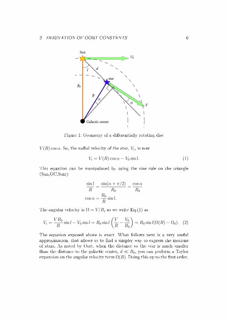
Fig. 1 shows how objects (stars) rotate dierentially in a disc. Dierentialrotation means that the angular velocity is a function of the radius. First,let's nd the radial component of a velocity for a star in a location depictedby the picture. The velocity of the Sun towards the star (the dotted line)is V0 cos(π/2 − l) = V0 sin l. The velocity of the star on the same line is

3 DERIVATION OF OORT CONSTANTS 6

Figure 1: Geometry of a dierentially rotating disc

V (R) cosα. So, the radial velocity of the star, Vr, is now

Vr = V (R) cosα− V0 sin l. (1)

This equation can be manipulated by using the sine rule on the triangle(Sun,GC,Star):

sin l

R=

sin(α + π/2)

R0

=cosα

R0

cosα =R0

Rsin l.

The angular velocity is Ω = V/R, so we write Eq.(1) as

Vr =V R0

Rsin l − V0 sin l = R0 sin l

(V

R− V0R0

)= R0 sin l(Ω(R) − Ω0). (2)

The equation exposed above is exact. What follows next is a very usefulapproximation, that allows us to nd a simpler way to express the motionsof stars. As noted by Oort, when the distance to the star is much smallerthan the distance to the galactic center, d R0, you can perform a Taylorexpansion on the angular velocity term Ω(R). Doing this up to the rst order,

3 DERIVATION OF OORT CONSTANTS 7

we obtain

Ω(R) = Ω0 +

(dΩ0

dR

)(R−R0)

Ω(R) − Ω0 =

[d

dR

(V (R)

R

)R0

](R−R0). (3)

Now we can write Eq.(2) as

Vr = R0 sin l

[d

dR

(V (R)

R

)R0

](R−R0). (4)

Because d is small, (R − R0) ≈ −d cos l, which follows from the cosine rule.Applying the rule to the same triangle as before we obtain

R2 = R20 + d2 − 2R0d cos l

R =√

(R20 + d2 − 2R0d cos l) = R0

√(1 + (d/R0)2 − 2(d/R0) cos l)

R ≈ R0

√1 − 2(d/R0) cos l) ≈ R0 − d cos l

R−R0 ≈ −d cos l, (5)

where the term (d/R0)2 ≈ 0 because d R0. Inserting Eq.(5) into Eq.(4),

and writing said equation a bit dierently we get

Vr =1

R0

d sin l cos l

[V0 −R0

(dV (R)

dR

)R0

]

= d sin l cos l

[V0R0

−(dV (R)

dR

)R0

]

= d sin(2l)1

2

[V0R0

−(dV (R)

dR

)R0

], (6)

orVr = Ad sin(2l), (7)

where A is the rst Oort constant

A =1

2

[V0R0

−(dV (R)

dR

)R0

].

3 DERIVATION OF OORT CONSTANTS 8

3.2 The Oort constant B

The velocity of the Sun and a star perpendicular to the dotted line in thepicture is V0 sin(π/2 − l) = V0 cos l and V (R) cos(π/2 − α) = V (R) sinα,respectively, so we get

Vt = V (R) sinα− V0 cos l. (8)

Also, let's look at the dotted line from GC that connects with the dottedline from the Sun through the star, and to which it is perpendicular. Let'smark this connection point as P. Now we have a triangle (Sun,GC,P). Thelength of the line from Sun to P is given by R0 cos l, but it is also given byd+R sinα, so we have

R0 cos l = d+R sinα

R sinα = R0 cos l − d. (9)

Inserting this into Eq.(8) we get

Vt =V (R)R0 cos l

R− V (R)d

R− V0 cos l

= R0 cos l

(V (R)

R− V0R0

)− V (R)

Rd. (10)

Using again the Taylor expansion and the fact that R − R0 = −d cos l, wecan write Eq.(10)

Vt ≈ d cos2 l

[V0R0

−(dV (R)

dR

)R0

]− V (R)

Rd. (11)

Using the identity cos(2l) = 2 cos2 l − 1, we can write Eq.(11) as

Vt ≈ d cos(2l)1

2

[V0R0

−(dV (R)

dR

)R0

]+

1

2d

[V0R0

−(dV (R)

dR

)R0

]− V0R0

d

Vt ≈ d[A cos(2l) + B], (12)

where B is the second Oort constant

B = −1

2

[V0R0

+

(dV (R)

dR

)R0

]. (13)

As can be seen from the constants, at least locally, the stars do not rotateabout the galactic centre as a solid body. If they did, and the angular velocitywere the same for every object, A = 0. As can be seen in the next chapter,this is not the case. These constants show that the rotation is dierential.

4 CALCULATING THE OORT CONSTANTS 9

4 Calculating the Oort constants

This work has made use of data from the European Space Agency (ESA)mission Gaia (https://www.cosmos.esa.int/gaia), processed by the GaiaData Processing and Analysis Consortium (DPAC, https://www.cosmos.esa.int/web/gaia/dpac/consortium). Funding for the DPAC has been pro-vided by national institutions, in particular the institutions participating inthe GaiaMultilateral Agreement. In particular, I've used the Gaia DR1 data,and information about the data and Gaia mission as a whole can be foundin papers[5][6].

In order to calculate the Oort Constants, I downloaded a table consistinglocal stars (distance < 500 pc), and for which the following attributes hadbeen observed: Right ascension, declination, parallax, proper motions for RAand Dec and Galactic longitude and latitude. I have also limited the data toonly include stars which are located in the galactic plane (−10 ≤ b ≤ 10).Because of this, the table included ∼ 266000 stars.

The way to obtain the constants is to plot the tangential velocity pro-jected in the galactic plane divided by the distance as a function of thegalactic longitude, or, Vt/d as a function of l. Then, to this plot, the functionA sin(2l) + B can be tted using the mpt procedure.

The required tangential velocity can be obtained from knowing the dis-tance and the proper motion on the galactic longitude axis, Vt = µld. It isimportant to note, that this tangential velocity includes the eect of Sun'smovement around the galactic centre. In other words, the Oort constants arecalculated with respect to the local standard of rest, LSR. So, in order tond the true tangential velocities, one must rst nd the velocity of the Sunwith respect to the LSR.

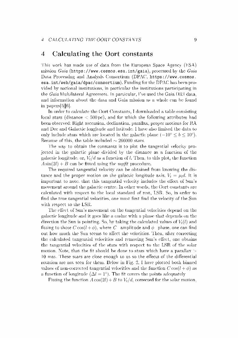
The eect of Sun's movement on the tangential velocities depend on thegalactic longitude and it goes like a cosine with a phase that depends on thedirection the Sun is pointing. So, by taking the calculated values of Vt(l) andtting to those C cos(l+φ), where C=amplitude and φ=phase, one can ndout how much the Sun seems to aect the velocities. Then, after correctingthe calculated tangential velocities and removing Sun's eect, one obtainsthe tangential velocities of the stars with respect to the LSR of the solarmotion. Note, that the t should be done to stars which have a parallax >10 mas. These stars are close enough to us so the eects of the dierentialrotation are not seen for them. Below in Fig. 2, I have plotted both binnedvalues of non-corrected tangential velocities and the function C cos(l+ φ) asa function of longitude (∆l = 1). The t covers the points adequately

Fitting the function A cos(2l) +B to Vt/d, corrected for the solar motion,

4 CALCULATING THE OORT CONSTANTS 10

Figure 2: Tangential velocities and a t C cos(l+φ) as a function of longitude.Bins made with ∆l = 1.

I obtained the following values for the constants:

A = 13.35 km s−1 kpc−1 (14)

B = −8.62 km s−1 kpc−1. (15)

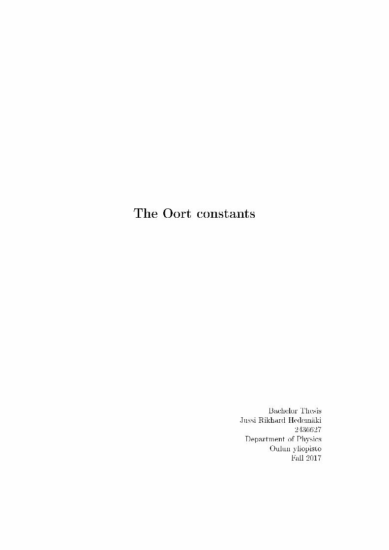
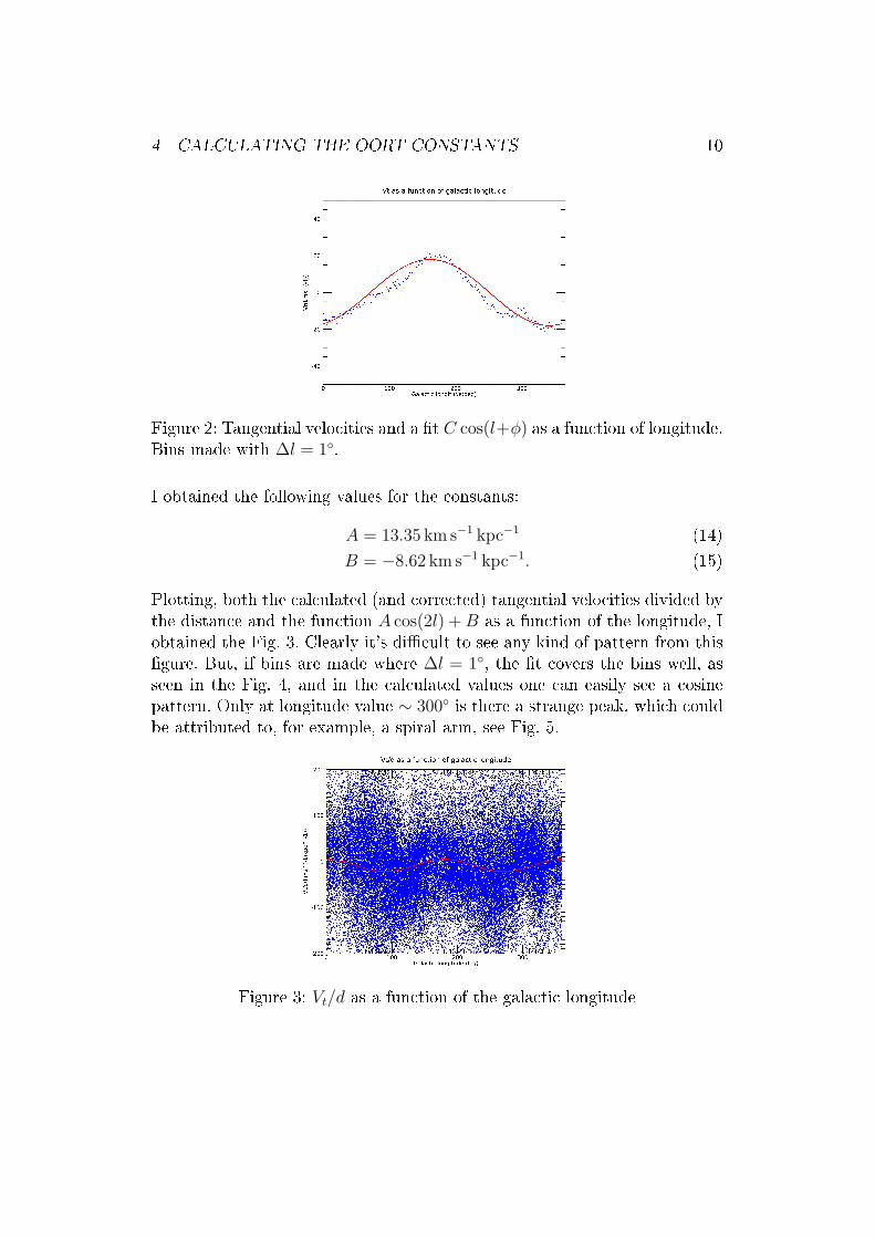
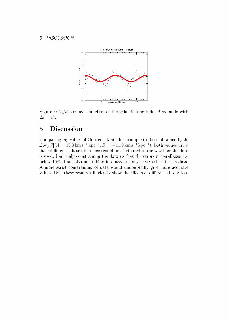
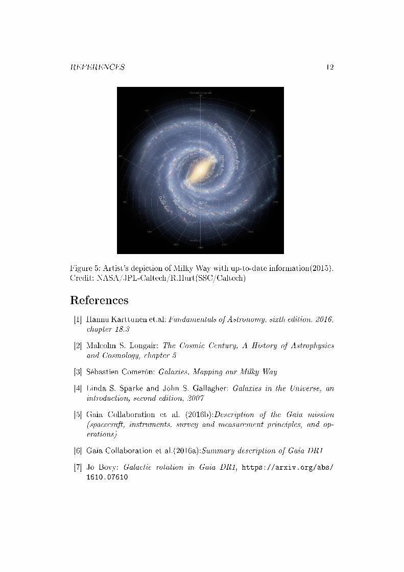
Plotting, both the calculated (and corrected) tangential velocities divided bythe distance and the function A cos(2l) +B as a function of the longitude, Iobtained the Fig. 3. Clearly it's dicult to see any kind of pattern from thisgure. But, if bins are made where ∆l = 1, the t covers the bins well, asseen in the Fig. 4, and in the calculated values one can easily see a cosinepattern. Only at longitude value ∼ 300 is there a strange peak, which couldbe attributed to, for example, a spiral arm, see Fig. 5.

Figure 3: Vt/d as a function of the galactic longitude

5 DISCUSSION 11

Figure 4: Vt/d bins as a function of the galactic longitude. Bins made with∆l = 1.

5 Discussion

Comparing my values of Oort constants, for example to those obtained by JoBovy[7](A = 15.3 km s−1 kpc−1, B = −11.9 km s−1 kpc−1), both values are alittle dierent. These dierences could be attributed to the way how the datais used. I am only constraining the data so that the errors in parallaxes arebelow 10%. I am also not taking into account any error values in the data.A more strict constraining of data would undoubtedly give more accuratevalues. But, these results still clearly show the eects of dierential rotation.

REFERENCES 12

Figure 5: Artist's depiction of Milky Way with up-to-date information(2015).Credit: NASA/JPL-Caltech/R.Hurt(SSC/Caltech)

References

[1] Hannu Karttunen et.al: Fundamentals of Astronomy, sixth edition, 2016,chapter 18.3

[2] Malcolm S. Longair: The Cosmic Century, A History of Astrophysicsand Cosmology, chapter 5

[3] Sébastien Comerón: Galaxies, Mapping our Milky Way

[4] Linda S. Sparke and John S. Gallagher: Galaxies in the Universe, anintroduction, second edition, 2007

[5] Gaia Collaboration et al. (2016b):Description of the Gaia mission(spacecraft, instruments, survey and measurement principles, and op-erations)

[6] Gaia Collaboration et al.(2016a):Summary description of Gaia DR1

[7] Jo Bovy: Galactic rotation in Gaia DR1, https://arxiv.org/abs/

1610.07610