The Optics Of Spectroscopy...2.3 Czerny Turner Configuration 2.4 Czerny Turner/Fastie Ebert PGS Aberrations 2.4.1 Aberration Correcting Plane Gratings 2.5 Concave Aberration Corrected

THE OPTICS OF SPECTROSCOPYA TUTORIAL By J.M. Lerner and A. Thevenon

TABLE OF CONTENTS

Section 1:DIFFRACTION GRATINGS RULED &HOLOGRAPHIC

1.1 Basic Equations●

1.2 Angular Dispersion●

1.3 Linear Dispersion●

1.4 Wavelength and Order●

1.5 Resolving "Power"●

1.6 Blazed Gratings

1.6.1 Littrow Condition❍

1.6.2 Efficiency Profiles❍

1.6.3 Efficiency and Order❍

●

1.7 Diffraction Grating Stray Light

1.7.1 Scattered Light❍

1.7.2 Ghosts❍

●

1.8 Choice of Gratings

1.8.1 When to Choose a Holographic Grating❍

1.8.2 When to Choose a Ruled Grating❍

●

Section 2:MONOCHROMATORS &SPECTROGRAPHS

2.1 Basic Designs●

2.2 FastieEbert Configuration●

2.3 CzernyTurner Configuration●

2.4 CzernyTurner/FastieEbert PGS Aberrations

2.4.1 Aberration Correcting Plane Gratings❍

●

2.5 Concave Aberration Corrected Holographic Gratings●

2.6 Calculating alpha and beta in a Monochromator Configuration●

The Optics Of Spectroscopy

file:///J|/isainc/OSD/OOS/OOSedited.HTM (1 of 4) [3/27/2002 9:35:27 AM]

2.7 Monochromator System Optics●

2.8 Aperture Stops and Entrance and Exit Pupils●

2.9 Aperture Ratio (f/value,F.Number),and Numerical Aperture (NA)

2.9.1 f/value of a Lens System❍

2.9.2 f/value of a Spectrometer❍

2.9.3 Magnification and Flux Density❍

●

2.10 Exit Slit Width and Anamorphism●

2.11 Slit Height Magnification●

2.12 Bandpass and Resolution

2.12.1 Influence of the Slits❍

2.12.2 Influence of Diffraction❍

2.12.3 Influence of Aberrations❍

2.12.4 Determination of the FWHM of the Instrumental Profile❍

2.12.5 Image Width and Array Detectors❍

2.12.6 Discussion of the Instrumental Profile❍

●

2.13 Order and Resolution●

2.14 Dispersion and Maximum Wavelength●

2.15 Order and Dispersion●

2.16 Choosing a Monochromator/Spectrograph●

Section 3: SPECTROMETER THROUGHPUT &ETENDUE

3.1 Definitions

3.1.1 Introduction to Etendue❍

●

3.2 Relative System Throughput

3.2.1 Calculation of the Etendue❍

●

3.3 Flux Entering the Spectrometer●

3.4 Example of Complete System Optimization with a Small Diameter Fiber Optic Light Source●

3.5 Example of Complete System Optimization with an Extended Light Source●

3.6 Variation of Throughput and Bandpass with Slit Widths

3.6.1 Continuous Spectral Source❍

3.6.2 Discrete Spectral Source❍

●



Section 4: OPTICAL SIGNALTONOISE RATIO ANDSTRAY LIGHT

4.1 Random Stray Light

4.1.1 Optical SignaltoNoise Ratio in a Spectrometer❍

4.1.2 The Quantification of Signal❍

4.1.3 The Quantification of Stray Light and S/N Ratio❍

4.1.4 Optimization of SignaltoNoise Ratio❍

4.1.5 Example of S/N Optimization❍

●

4.2 Directional Stray Light

4.2.1 Incorrect Illumination of the Spectrometer❍

4.2.2 Reentry Spectra❍

4.2.3 Grating Ghosts❍

●

4.3 S/N Ratio and Slit Dimensions

4.3.1 The Case for a SINGLE Monochromator and a CONTINUUM Light Source❍

4.3.2 The Case for a SINGLE Monochromator and MONOCHROMATIC Light❍

4.3.3 The Case for a DOUBLE Monochromator and a CONTINUUM Light Source❍

4.3.4 The Case for a DOUBLE Monochromator and a MONOCHROMATIC Light Source❍

●

Section 5: THE RELATIONSHIP BETWEENWAVELENGTH AND PIXEL POSITION ON ANARRAY

5.1 The Determination of Wavelength at a Given Location on a Focal Plane

5.1.1 Discussion of Results❍

5.1.2 Determination of the Position of a Known Wavelength in the Focal Plane❍

●

Section 6: ENTRANCE OPTICS

6.1 Choice of Entrance Optics

6.1.1 Review of Basic Equations❍

●

6.2 Establishing the Optical Axis of the Monochromator System

6.2.1. Materials❍

6.2.2 Procedure❍

●



6.3 Illuminating a Spectrometer●

6.4 Entrance Optics Examples

6.4.1 Aperture Matching a Small Source❍

6.4.2 Aperture Matching an Extended Source❍

6.4.3 Demagnifying a Source❍

●

6.5 Use of Field Lenses●

6.6 Pinhole Camera Effect●

6.7 Spatial Filters●

References



Section 1: Diffraction Gratings Ruled &Holographic

Diffraction gratings are manufactured either classically with the use of a ruling engine by burnishinggrooves with a diamond stylus or holographically with the use of interference fringes generated at theintersection of two laser beams. (For more details see Diffraction Gratings Ruled & HolographicHandbook, Reference 1.)

Classically ruled gratings may be plano or concave and possess grooves each parallel with the next.Holographic grating grooves may be either parallel or of unequal distribution in order that systemperformance may be optimized. Holographic gratings are generated on plano, spherical, toroidal, andmany other surfaces.

Regardless of the shape of the surface or whether classically ruled or holographic, the text that follows isequally applicable to each. Where there are differences, these are explained.

1.1 Basic EquationsBefore introducing the basic equations, a brief note on monochromatic light and continuous spectra mustfirst be considered.

Monochromatic light has infinitely narrow spectral width. Good sources which approximate such lightinclude single mode lasers and very low pressure, cooled spectral calibration lamps. These are alsovariously known as "line" or "discrete line" sources.

A continuous spectrum has finite spectral width, e.g. "white light". In principle all wavelengths arepresent, but in practice a "continuum" is almost always a segment of a spectrum. Sometimes a continuousspectral segment may be only a few parts of a nanometer wide and resemble a line spectrum.

The equations that follow are for systems in air where µ0 = 1. Therefore,λ = λ0 = wavelength in air.

Definitions Units

alpha - angle of incidence degreesbeta - angle of diffraction degreesk - diffraction order integern - groove density grooves/mmDV - the included angle degrees (or deviation angle)µ0 - refractive indexλ - wavelength in vacuum nanometers (nary)λ0 - wavelength in medium of refractive index, µ0, where λ0 = λm0

1 nm = 10-6 mm; 1 micrometer = 10-3 mm; 1 A = 10-7 mm

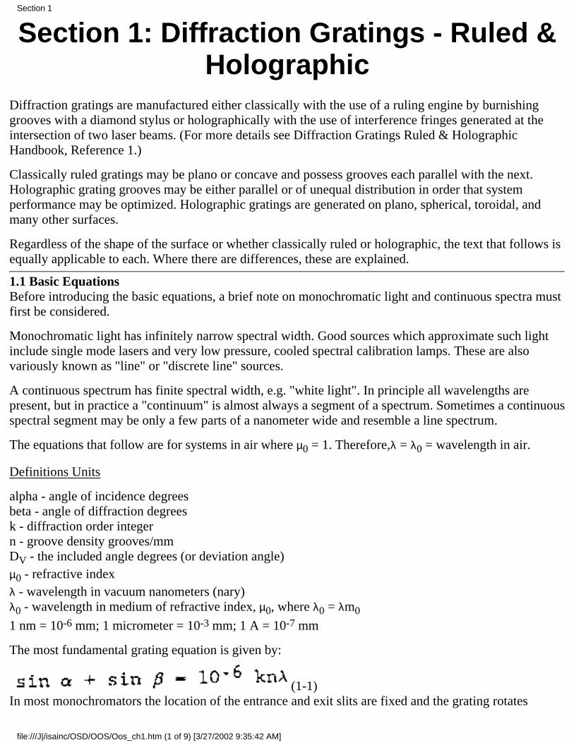
The most fundamental grating equation is given by:

(11)In most monochromators the location of the entrance and exit slits are fixed and the grating rotates

Section 1

file:///J|/isainc/OSD/OOS/Oos_ch1.htm (1 of 9) [3/27/2002 9:35:42 AM]

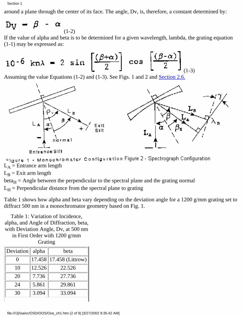
around a plane through the center of its face. The angle, Dv, is, therefore, a constant determined by:

(12)If the value of alpha and beta is to be determined for a given wavelength, lambda, the grating equation(11) may be expressed as:

(1-3)Assuming the value Equations (12) and (1-3). See Figs. 1 and 2 and Section 2.6.

LA = Entrance arm lengthLB = Exit arm lengthbetaH = Angle between the perpendicular to the spectral plane and the grating normalLH = Perpendicular distance from the spectral plane to grating

Table 1 shows how alpha and beta vary depending on the deviation angle for a 1200 g/mm grating set todiffract 500 nm in a monochromator geometry based on Fig. 1.

Table 1: Variation of Incidence,alpha, and Angle of Diffraction, beta,with Deviation Angle, Dv, at 500 nm

in First Order with 1200 g/mmGrating

Deviation alpha beta

0 17.458 17.458 (Littrow)

10 12.526 22.526

20 7.736 27.736

24 5.861 29.861

30 3.094 33.094

Section 1


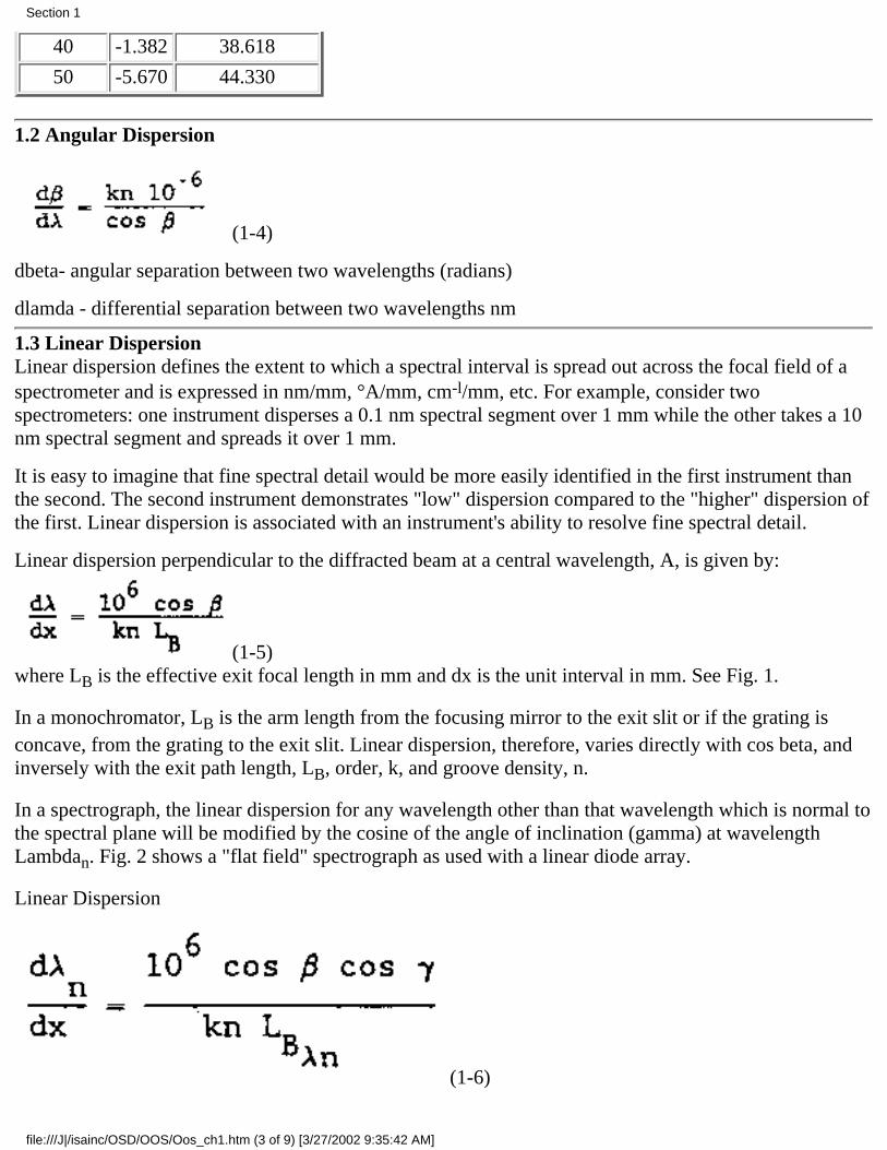
40 -1.382 38.618

50 -5.670 44.330

1.2 Angular Dispersion

(14)

dbeta angular separation between two wavelengths (radians)

dlamda differential separation between two wavelengths nm

1.3 Linear DispersionLinear dispersion defines the extent to which a spectral interval is spread out across the focal field of aspectrometer and is expressed in nm/mm, °A/mm, cm-l/mm, etc. For example, consider twospectrometers: one instrument disperses a 0.1 nm spectral segment over 1 mm while the other takes a 10nm spectral segment and spreads it over 1 mm.

It is easy to imagine that fine spectral detail would be more easily identified in the first instrument thanthe second. The second instrument demonstrates "low" dispersion compared to the "higher" dispersion ofthe first. Linear dispersion is associated with an instrument's ability to resolve fine spectral detail.

Linear dispersion perpendicular to the diffracted beam at a central wavelength, A, is given by:

(15)where LB is the effective exit focal length in mm and dx is the unit interval in mm. See Fig. 1.

In a monochromator, LB is the arm length from the focusing mirror to the exit slit or if the grating isconcave, from the grating to the exit slit. Linear dispersion, therefore, varies directly with cos beta, andinversely with the exit path length, LB, order, k, and groove density, n.

In a spectrograph, the linear dispersion for any wavelength other than that wavelength which is normal tothe spectral plane will be modified by the cosine of the angle of inclination (gamma) at wavelengthLambdan. Fig. 2 shows a "flat field" spectrograph as used with a linear diode array.

Linear Dispersion

(16)

Section 1


(17)

(18)

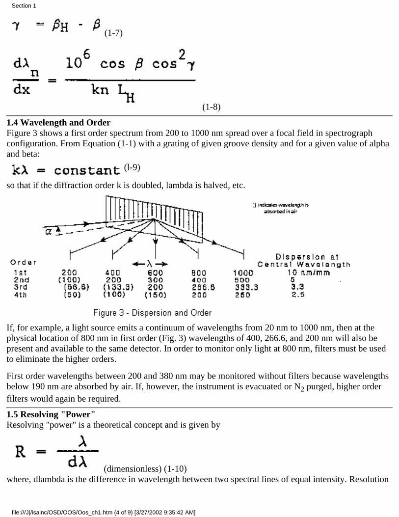
1.4 Wavelength and OrderFigure 3 shows a first order spectrum from 200 to 1000 nm spread over a focal field in spectrographconfiguration. From Equation (11) with a grating of given groove density and for a given value of alphaand beta:

(l9)

so that if the diffraction order k is doubled, lambda is halved, etc.

If, for example, a light source emits a continuum of wavelengths from 20 nm to 1000 nm, then at thephysical location of 800 nm in first order (Fig. 3) wavelengths of 400, 266.6, and 200 nm will also bepresent and available to the same detector. In order to monitor only light at 800 nm, filters must be usedto eliminate the higher orders.

First order wavelengths between 200 and 380 nm may be monitored without filters because wavelengthsbelow 190 nm are absorbed by air. If, however, the instrument is evacuated or N2 purged, higher orderfilters would again be required.

1.5 Resolving "Power"Resolving "power" is a theoretical concept and is given by

(dimensionless) (110)where, dlambda is the difference in wavelength between two spectral lines of equal intensity. Resolution

Section 1


is then the ability of the instrument to separate adjacent spectral lines. Two peaks are considered resolvedif the distance between them is such that the maximum of one falls on the first minimum of the other.This is called the Rayleigh criterion.

It may be shown that:

(111)

lambda - the central wavelength of the spectral line to be resolved

Wg the illuminated width of the grating

N the total number of grooves on the grating

The numerical resolving power "R" should not be confused with the resolution or bandpass of aninstrument system (See Section 2).

Theoretically, a 1200 g/mm grating with a width of 110 mm that is used in first order has a numericalresolving power R = 1200 x 110 = 132,000. Therefore, at 500 nm, the bandpass

In a real instrument, however, the geometry of use is fixed by Equation (11). Solving for k:

(112)

But the ruled width, Wg, of the grating:

(113)

where (114)

after substitution of (112) and (113) in (111).

Resolving power may also be expressed as:

Section 1


(115)

Consequently, the resolving power of a grating is dependent on:

* The width of the grating

* The center wavelength to be resolved

* The geometry of the use conditions

Because bandpass is also determined by the slit width of the spectrometer and residual systemaberrations, an achieved bandpass at this level is only possible in diffraction limited instrumentsassuming an unlikely 100% of theoretical. See Section 2 for further discussion.

1.6 Blazed GratingsBlaze: The concentration of a limited region of the spectrum into any order other than the zero order.Blazed gratings are manufactured to produce maximum efficiency at designated wavelengths. A gratingmay, therefore, be described as "blazed at 250 nm" or "blazed at 1 micron" etc. by appropriate selectionof groove geometry.

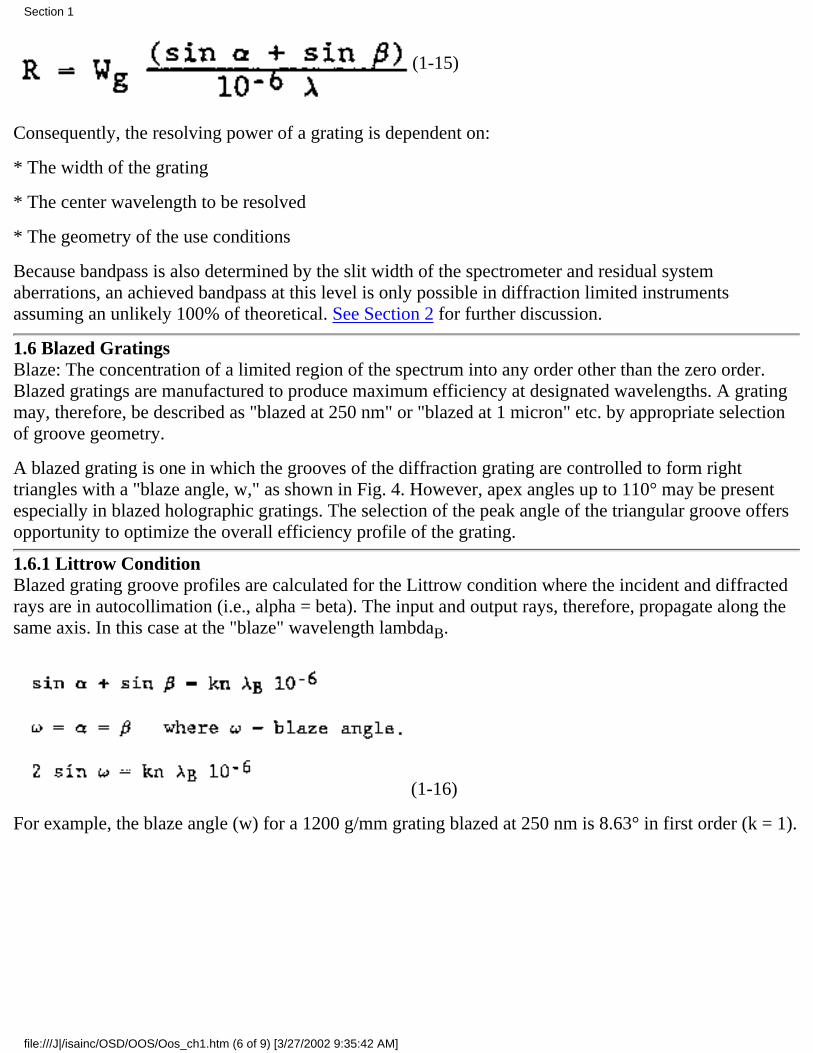
A blazed grating is one in which the grooves of the diffraction grating are controlled to form righttriangles with a "blaze angle, w," as shown in Fig. 4. However, apex angles up to 110° may be presentespecially in blazed holographic gratings. The selection of the peak angle of the triangular groove offersopportunity to optimize the overall efficiency profile of the grating.

1.6.1 Littrow ConditionBlazed grating groove profiles are calculated for the Littrow condition where the incident and diffractedrays are in autocollimation (i.e., alpha = beta). The input and output rays, therefore, propagate along thesame axis. In this case at the "blaze" wavelength lambdaB.

(116)

For example, the blaze angle (w) for a 1200 g/mm grating blazed at 250 nm is 8.63° in first order (k = 1).

Section 1


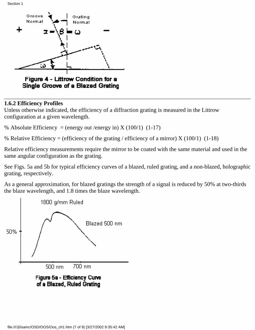
1.6.2 Efficiency ProfilesUnless otherwise indicated, the efficiency of a diffraction grating is measured in the Littrowconfiguration at a given wavelength.

% Absolute Efficiency = (energy out /energy in) X (100/1) (117)

% Relative Efficiency = (efficiency of the grating / efficiency of a mirror) X (100/1) (1-18)

Relative efficiency measurements require the mirror to be coated with the same material and used in thesame angular configuration as the grating.

See Figs. 5a and 5b for typical efficiency curves of a blazed, ruled grating, and a nonblazed, holographicgrating, respectively.

As a general approximation, for blazed gratings the strength of a signal is reduced by 50% at twothirdsthe blaze wavelength, and 1.8 times the blaze wavelength.

Section 1


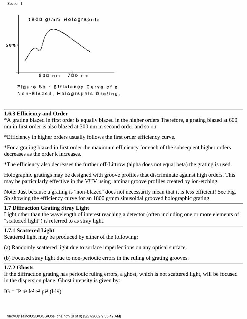
1.6.3 Efficiency and Order*A grating blazed in first order is equally blazed in the higher orders Therefore, a grating blazed at 600nm in first order is also blazed at 300 nm in second order and so on.

*Efficiency in higher orders usually follows the first order efficiency curve.

*For a grating blazed in first order the maximum efficiency for each of the subsequent higher ordersdecreases as the order k increases.

*The efficiency also decreases the further offLittrow (alpha does not equal beta) the grating is used.

Holographic gratings may be designed with groove profiles that discriminate against high orders. Thismay be particularly effective in the VUV using laminar groove profiles created by ionetching.

Note: Just because a grating is "nonblazed" does not necessarily mean that it is less efficient! See Fig.Sb showing the efficiency curve for an 1800 g/mm sinusoidal grooved holographic grating.

1.7 Diffraction Grating Stray LightLight other than the wavelength of interest reaching a detector (often including one or more elements of"scattered light") is referred to as stray light.

1.7.1 Scattered LightScattered light may be produced by either of the following:

(a) Randomly scattered light due to surface imperfections on any optical surface.

(b) Focused stray light due to nonperiodic errors in the ruling of grating grooves.

1.7.2 GhostsIf the diffraction grating has periodic ruling errors, a ghost, which is not scattered light, will be focusedin the dispersion plane. Ghost intensity is given by:

IG = IP n2 k2 e2 pi2 (ll9)

Section 1


where,

IG =ghost intensity

IP = parent intensity

n = groove density

k =order

e =error in the position of the grooves

Ghosts are focused and imaged in the dispersion plane of the monochromator.●

Stray light of a holographic grating is usually up to a factor of ten times less than that of aclassically ruled grating, typically nonfocused, and when present, radiates through 2pi steradians.

●

Holographic gratings show no ghosts because there are no periodic ruling errors and, therefore,often represent the best solution to ghost problems.

●

1.8 Choice of Gratings

1.8.1 Uhen to Choose a Holographic Grating(1) When grating is concave.(2) When laser light is present, e.g., Raman, laser fluorescence, etc.(3) Any time groove density should be 1200 g/mm or more (up to 6000 g/mm and 120 mm x 140 mm insize) for use in near UV , VIS, and near IR.(4) When working in the W below 200 nm down to 3 nm.(5) For high resolution when high groove density will be superior to a low groove density grating used inhigh order (k > 1).(6) Whenever an ionetched holographic grating is available.

1.8.2 When to Choose a Ruled Grating(1) When working in IR above 1.2 um, if an ionetched holographic grating is unavailable.(2) When working with very low groove density, e.g., less than 600 g/mm.

Remember, ghosts and subsequent stray light intensity are proportional to the square of order and groovedensity (n2 and k2 from Equation (118)). Beware of using ruled gratings in high order or with highgroove density.

[Go to Section 2] [Return to Table of Contents]

Section 1


Section 2:Monochromators &Spectrographs

2.1 Basic DesignsMonochromator and spectrograph systems form an image of the entrance slit in the exit plane at the wavelengthspresent in the light source. There are numerous configurations by which this may be achieved -- only the mostcommon are discussed in this document and includes Plane Grating Systems (PGS) and Aberration CorrectedHolographic Grating (ACHG) systems.

DefinitionsLA - entrance arm lengthLB - exit arm lengthh - height of entrance slith' - height of image of the entrance slitalpha - angle of incidencebeta - angle of diffractionw - width of entrance slitw' - width of entrance slit imageDg - diameter of a circular gratingWg - width of a rectangular gratingHg - height of a rectangular grating

2.2 Fastie-Ebert ConfigurationA Fastie-Ebert instrument consists of one large spherical mirror and one plane diffraction grating (see Fig. 6).

A portion of the mirror first collimates the light which will fall upon the plane grating. A separate portion of themirror then focuses the dispersed light from the grating into images of the entrance slit in the exit plane.

It is an inexpensive and commonly used design, but exhibits limited ability to maintain image quality offaxisdue to system aberrations such as spherical aberration, coma, astigmatism, and a curved focal field.

Section 2

file:///J|/isainc/OSD/OOS/OOS_CH2.HTM (1 of 19) [3/27/2002 9:36:02 AM]

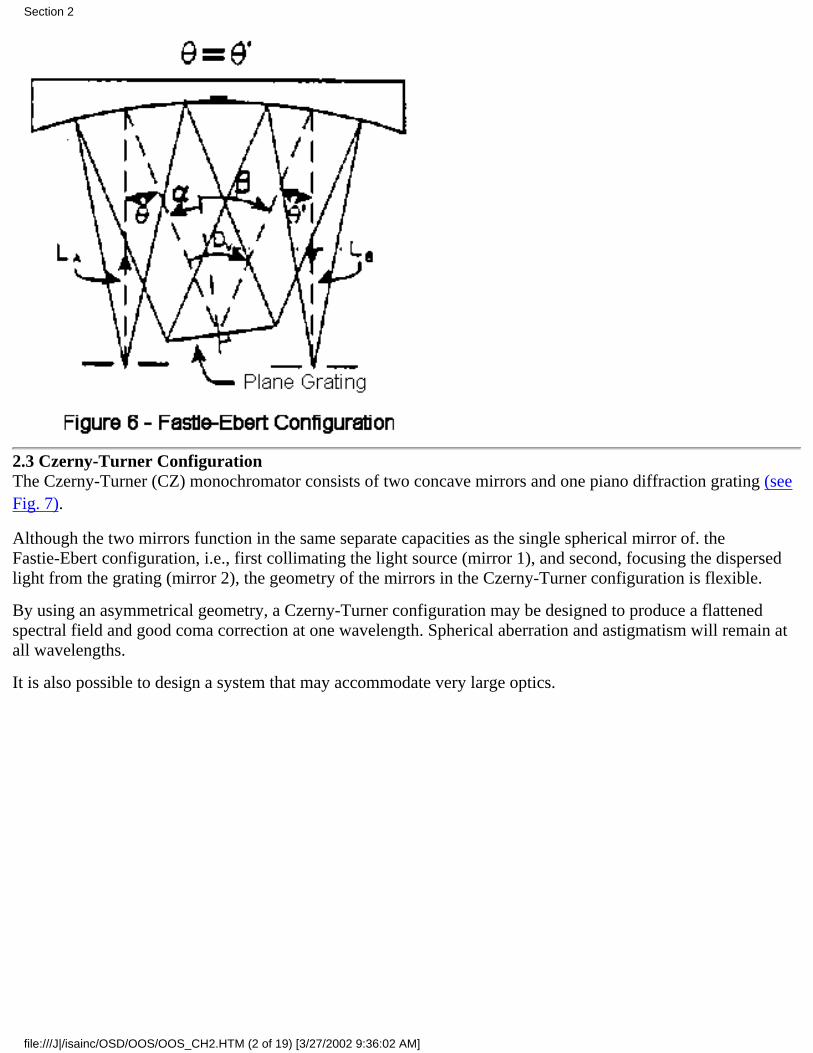
2.3 Czerny-Turner ConfigurationThe Czerny-Turner (CZ) monochromator consists of two concave mirrors and one piano diffraction grating (seeFig. 7).

Although the two mirrors function in the same separate capacities as the single spherical mirror of. theFastie-Ebert configuration, i.e., first collimating the light source (mirror 1), and second, focusing the dispersedlight from the grating (mirror 2), the geometry of the mirrors in the Czerny-Turner configuration is flexible.

By using an asymmetrical geometry, a Czerny-Turner configuration may be designed to produce a flattenedspectral field and good coma correction at one wavelength. Spherical aberration and astigmatism will remain atall wavelengths.

It is also possible to design a system that may accommodate very large optics.

Section 2


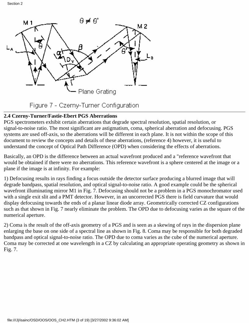
2.4 Czerny-Turner/Fastie-Ebert PGS AberrationsPGS spectrometers exhibit certain aberrations that degrade spectral resolution, spatial resolution, orsignaltonoise ratio. The most significant are astigmatism, coma, spherical aberration and defocusing. PGSsystems are used offaxis, so the aberrations will be different in each plane. It is not within the scope of thisdocument to review the concepts and details of these aberrations, (reference 4) however, it is useful tounderstand the concept of Optical Path Difference (OPD) when considering the effects of aberrations.

Basically, an OPD is the difference between an actual wavefront produced and a "reference wavefront thatwould be obtained if there were no aberrations. This reference wavefront is a sphere centered at the image or aplane if the image is at infinity. For example:

1) Defocusing results in rays finding a focus outside the detector surface producing a blurred image that willdegrade bandpass, spatial resolution, and optical signal-to-noise ratio. A good example could be the sphericalwavefront illuminating mirror M1 in Fig. 7. Defocusing should not be a problem in a PGS monochromator usedwith a single exit slit and a PMT detector. However, in an uncorrected PGS there is field curvature that woulddisplay defocusing towards the ends of a planar linear diode array. Geometrically corrected CZ configurationssuch as that shown in Fig. 7 nearly eliminate the problem. The OPD due to defocusing varies as the square of thenumerical aperture.

2) Coma is the result of the off-axis geometry of a PGS and is seen as a skewing of rays in the dispersion planeenlarging the base on one side of a spectral line as shown in Fig. 8. Coma may be responsible for both degradedbandpass and optical signal-to-noise ratio. The OPD due to coma varies as the cube of the numerical aperture.Coma may be corrected at one wavelength in a CZ by calculating an appropriate operating geometry as shown inFig. 7.

Section 2


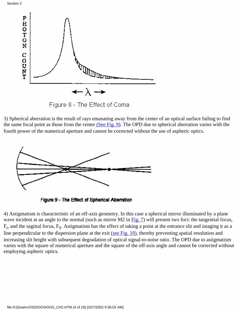
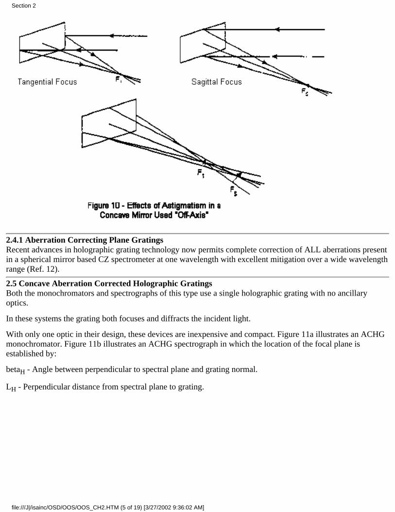
3) Spherical aberration is the result of rays emanating away from the center of an optical surface failing to findthe same focal point as those from the center (See Fig. 9). The OPD due to spherical aberration varies with thefourth power of the numerical aperture and cannot be corrected without the use of aspheric optics.

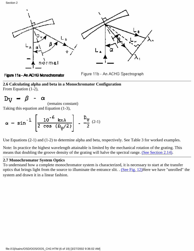
4) Astigmatism is characteristic of an off-axis geometry. In this case a spherical mirror illuminated by a planewave incident at an angle to the normal (such as mirror M2 in Fig. 7) will present two foci: the tangential focus,Ft, and the sagittal focus, FS. Astigmatism has the effect of taking a point at the entrance slit and imaging it as aline perpendicular to the dispersion plane at the exit (see Fig. 10), thereby preventing spatial resolution andincreasing slit height with subsequent degradation of optical signaltonoise ratio. The OPD due to astigmatismvaries with the square of numerical aperture and the square of the offaxis angle and cannot be corrected withoutemploying aspheric optics.

Section 2


2.4.1 Aberration Correcting Plane GratingsRecent advances in holographic grating technology now permits complete correction of ALL aberrations presentin a spherical mirror based CZ spectrometer at one wavelength with excellent mitigation over a wide wavelengthrange (Ref. 12).

2.5 Concave Aberration Corrected Holographic GratingsBoth the monochromators and spectrographs of this type use a single holographic grating with no ancillaryoptics.

In these systems the grating both focuses and diffracts the incident light.

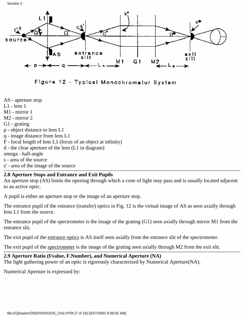
With only one optic in their design, these devices are inexpensive and compact. Figure 11a illustrates an ACHGmonochromator. Figure 11b illustrates an ACHG spectrograph in which the location of the focal plane isestablished by:

betaH - Angle between perpendicular to spectral plane and grating normal.

LH - Perpendicular distance from spectral plane to grating.

Section 2


2.6 Calculating alpha and beta in a Monochromator ConfigurationFrom Equation (1-2),

(remains constant)Taking this equation and Equation (1-3),

(21)

Use Equations (21) and (12) to determine alpha and beta, respectively. See Table 3 for worked examples.

Note: In practice the highest wavelength attainable is limited by the mechanical rotation of the grating. Thismeans that doubling the groove density of the grating will halve the spectral range. (See Section 2.14).

2.7 Monochromator System OpticsTo understand how a complete monochromator system is characterized, it is necessary to start at the transferoptics that brings light from the source to illuminate the entrance slit. . (See Fig. 12)Here we have "unrolled" thesystem and drawn it in a linear fashion.

Section 2


AS - aperture stopL1 - lens 1M1 - mirror 1M2 - mirror 2G1 - gratingp - object distance to lens L1q - image distance from lens L1F - focal length of lens L1 (focus of an object at infinity)d - the clear aperture of the lens (L1 in diagram)omega - half-angles - area of the sources' - area of the image of the source

2.8 Aperture Stops and Entrance and Exit PupilsAn aperture stop (AS) limits the opening through which a cone of light may pass and is usually located adjacentto an active optic.

A pupil is either an aperture stop or the image of an aperture stop.

The entrance pupil of the entrance (transfer) optics in Fig. 12 is the virtual image of AS as seen axially throughlens L1 from the source.

The entrance pupil of the spectrometer is the image of the grating (G1) seen axially through mirror M1 from theentrance slit.

The exit pupil of the entrance optics is AS itself seen axially from the entrance slit of the spectrometer.

The exit pupil of the spectrometer is the image of the grating seen axially through M2 from the exit slit.

2.9 Aperture Ratio (f/value, F.Number), and Numerical Aperture (NA)The light gathering power of an optic is rigorously characterized by Numerical Aperture(NA).

Numerical Aperture is expressed by:

Section 2


(22)

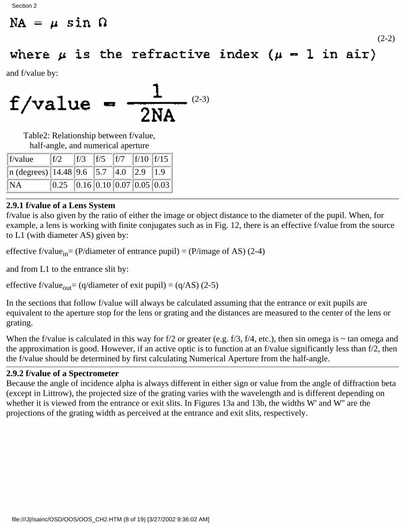
and f/value by:

(23)

Table2: Relationship between f/value,half-angle, and numerical aperture

f/value f/2 f/3 f/5 f/7 f/10 f/15

n (degrees) 14.48 9.6 5.7 4.0 2.9 1.9

NA 0.25 0.16 0.10 0.07 0.05 0.03

2.9.1 f/value of a Lens Systemf/value is also given by the ratio of either the image or object distance to the diameter of the pupil. When, forexample, a lens is working with finite conjugates such as in Fig. 12, there is an effective f/value from the sourceto L1 (with diameter AS) given by:

effective f/valuein= (P/diameter of entrance pupil) = (P/image of AS) (24)

and from L1 to the entrance slit by:

effective f/valueout= (q/diameter of exit pupil) = (q/AS) (25)

In the sections that follow f/value will always be calculated assuming that the entrance or exit pupils areequivalent to the aperture stop for the lens or grating and the distances are measured to the center of the lens orgrating.

When the f/value is calculated in this way for f/2 or greater (e.g. f/3, f/4, etc.), then sin omega is ~ tan omega andthe approximation is good. However, if an active optic is to function at an f/value significantly less than f/2, thenthe f/value should be determined by first calculating Numerical Aperture from the half-angle.

2.9.2 f/value of a SpectrometerBecause the angle of incidence alpha is always different in either sign or value from the angle of diffraction beta(except in Littrow), the projected size of the grating varies with the wavelength and is different depending onwhether it is viewed from the entrance or exit slits. In Figures 13a and 13b, the widths W' and W'' are theprojections of the grating width as perceived at the entrance and exit slits, respectively.

Section 2


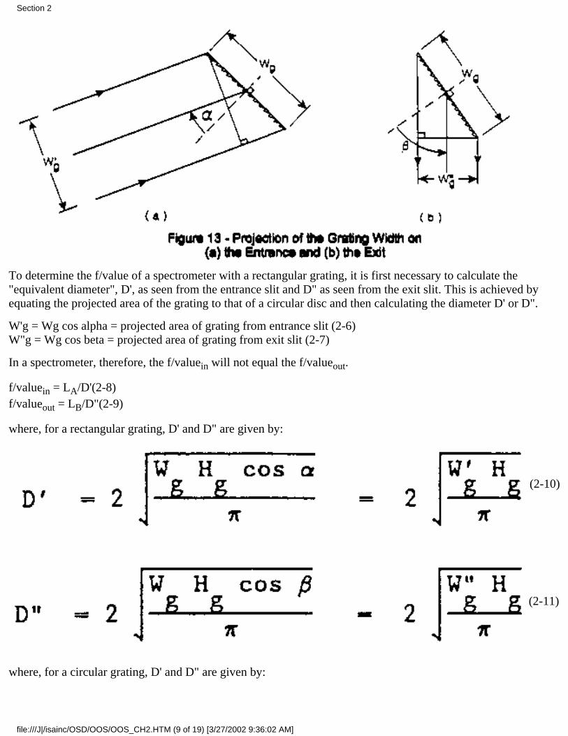
To determine the f/value of a spectrometer with a rectangular grating, it is first necessary to calculate the"equivalent diameter", D', as seen from the entrance slit and D" as seen from the exit slit. This is achieved byequating the projected area of the grating to that of a circular disc and then calculating the diameter D' or D".

W'g = Wg cos alpha = projected area of grating from entrance slit (26)W"g = Wg cos beta = projected area of grating from exit slit (27)

In a spectrometer, therefore, the f/valuein will not equal the f/valueout.

f/valuein = LA/D'(28)f/valueout = LB/D"(29)

where, for a rectangular grating, D' and D" are given by:

(210)

(211)

where, for a circular grating, D' and D" are given by:

Section 2


D' = Dg(cos alpha)^(1/2) (212)D" = Dg(cos beta)^(1/2) (213)

Table 3 shows how the f/value changes with wavelength.

Table 3 Calculated values for f/valuein and f/valueout for a Czerny-Turner configuration with 68 x 68 mm, 1800g/mm grating and LA = LB = F = 320 nm. Dv = 24 °.

Lambda(nm) alpha beta f/valuein f/valueout

200 1.40 22.60 4.17 4.34

320 5.12 29.12 4.18 4.46

500 15.39 39.39 4.25 4.74

680 26.73 50.73 4.41 5.24

800 35.40 59.40 4.62 5.84

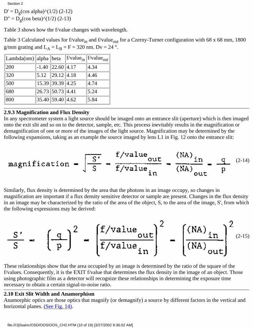
2.9.3 Magnification and Flux DensityIn any spectrometer system a light source should be imaged onto an entrance slit (aperture) which is then imagedonto the exit slit and so on to the detector, sample, etc. This process inevitably results in the magnification ordemagnification of one or more of the images of the light source. Magnification may be determined by thefollowing expansions, taking as an example the source imaged by lens L1 in Fig. 12 onto the entrance slit:

(214)

Similarly, flux density is determined by the area that the photons in an image occupy, so changes inmagnification are important if a flux density sensitive detector or sample are present. Changes in the flux densityin an image may be characterized by the ratio of the area of the object, S, to the area of the image, S', from whichthe following expressions may be derived:

(215)

These relationships show that the area occupied by an image is determined by the ratio of the square of thef/values. Consequently, it is the EXIT f/value that determines the flux density in the image of an object. Thoseusing photographic film as a detector will recognize these relationships in determining the exposure timenecessary to obtain a certain signal-to-noise ratio.

2.10 Exit Slit Width and AnamorphismAnamorphic optics are those optics that magnify (or demagnify) a source by different factors in the vertical andhorizontal planes. (See Fig. 14).

Section 2


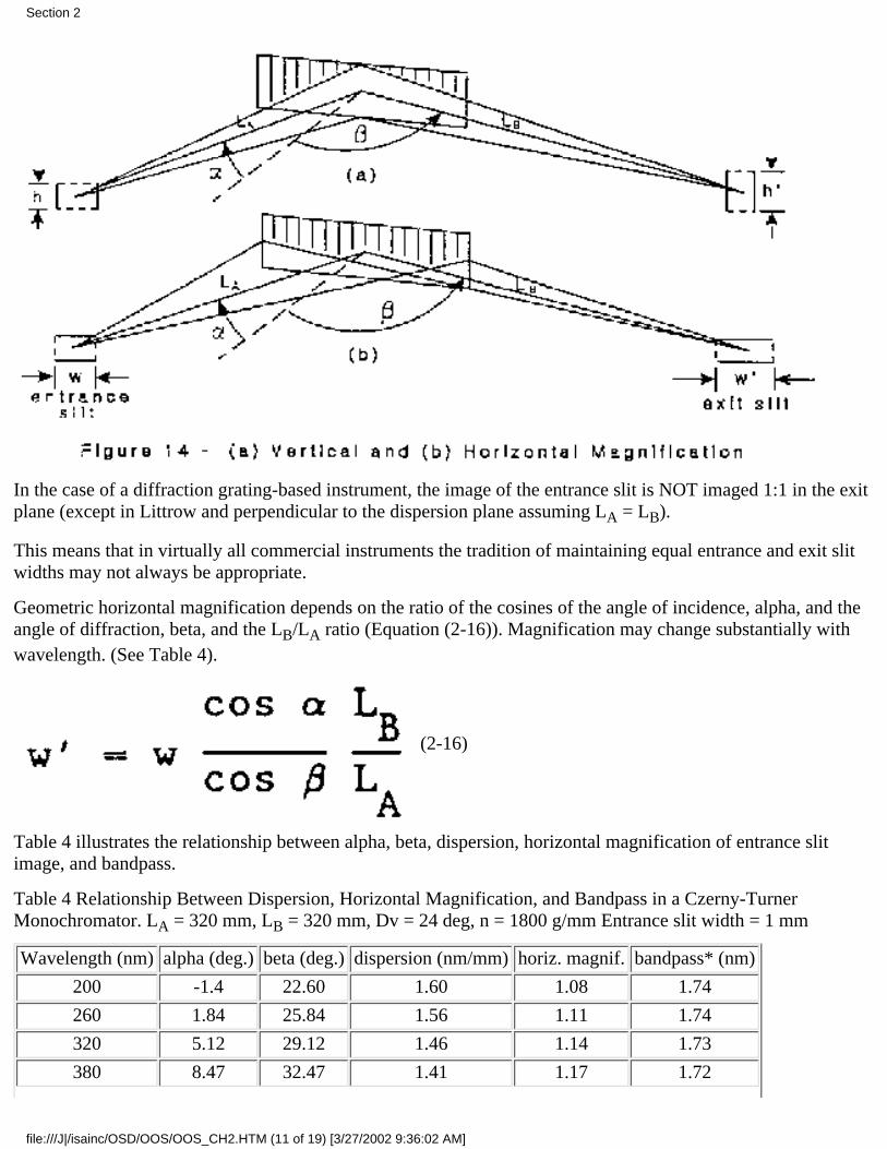
In the case of a diffraction grating-based instrument, the image of the entrance slit is NOT imaged 1:1 in the exitplane (except in Littrow and perpendicular to the dispersion plane assuming LA = LB).

This means that in virtually all commercial instruments the tradition of maintaining equal entrance and exit slitwidths may not always be appropriate.

Geometric horizontal magnification depends on the ratio of the cosines of the angle of incidence, alpha, and theangle of diffraction, beta, and the LB/LA ratio (Equation (216)). Magnification may change substantially withwavelength. (See Table 4).

(216)

Table 4 illustrates the relationship between alpha, beta, dispersion, horizontal magnification of entrance slitimage, and bandpass.

Table 4 Relationship Between Dispersion, Horizontal Magnification, and Bandpass in a CzernyTurnerMonochromator. LA = 320 mm, LB = 320 mm, Dv = 24 deg, n = 1800 g/mm Entrance slit width = 1 mm

Wavelength (nm) alpha (deg.) beta (deg.) dispersion (nm/mm) horiz. magnif. bandpass* (nm)

200 -1.4 22.60 1.60 1.08 1.74

260 1.84 25.84 1.56 1.11 1.74

320 5.12 29.12 1.46 1.14 1.73

380 8.47 32.47 1.41 1.17 1.72

Section 2


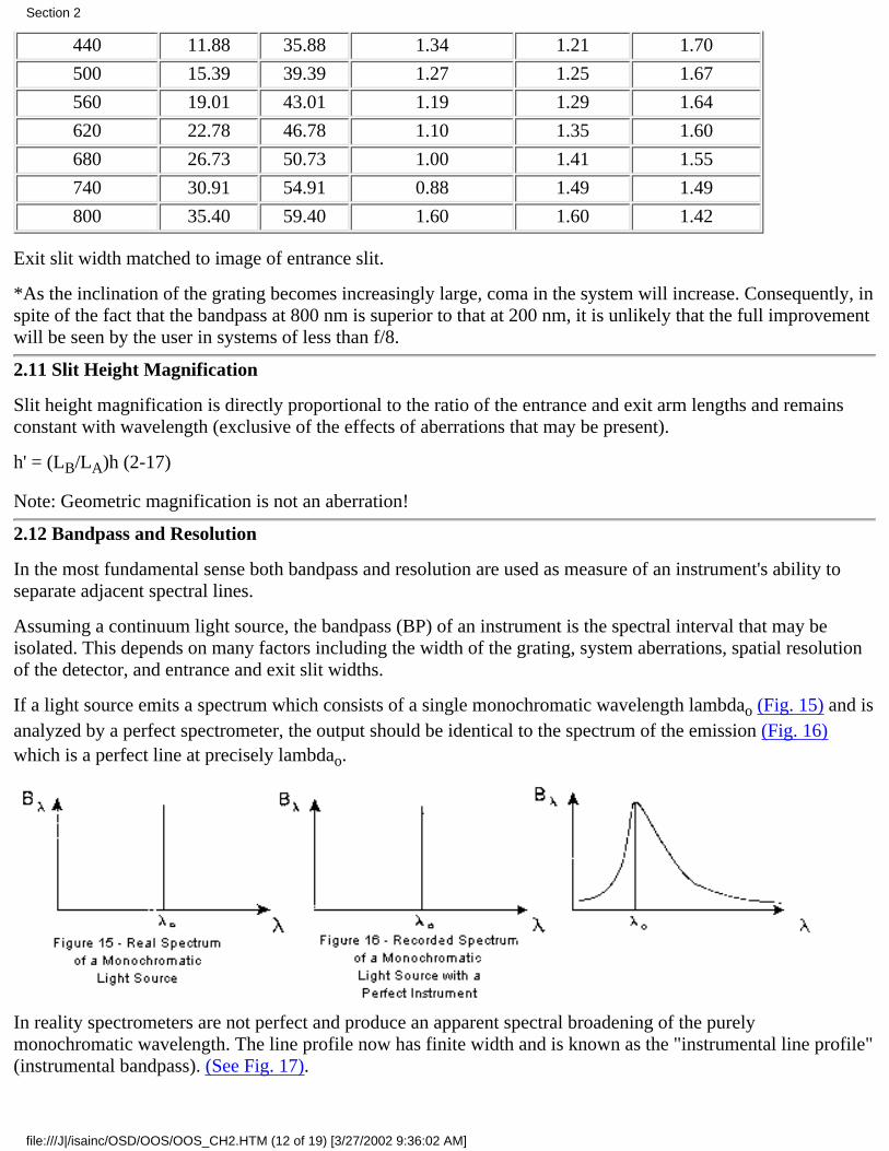
440 11.88 35.88 1.34 1.21 1.70

500 15.39 39.39 1.27 1.25 1.67

560 19.01 43.01 1.19 1.29 1.64

620 22.78 46.78 1.10 1.35 1.60

680 26.73 50.73 1.00 1.41 1.55

740 30.91 54.91 0.88 1.49 1.49

800 35.40 59.40 1.60 1.60 1.42

Exit slit width matched to image of entrance slit.

*As the inclination of the grating becomes increasingly large, coma in the system will increase. Consequently, inspite of the fact that the bandpass at 800 nm is superior to that at 200 nm, it is unlikely that the full improvementwill be seen by the user in systems of less than f/8.

2.11 Slit Height Magnification

Slit height magnification is directly proportional to the ratio of the entrance and exit arm lengths and remainsconstant with wavelength (exclusive of the effects of aberrations that may be present).

h' = (LB/LA)h (217)

Note: Geometric magnification is not an aberration!

2.12 Bandpass and Resolution

In the most fundamental sense both bandpass and resolution are used as measure of an instrument's ability toseparate adjacent spectral lines.

Assuming a continuum light source, the bandpass (BP) of an instrument is the spectral interval that may beisolated. This depends on many factors including the width of the grating, system aberrations, spatial resolutionof the detector, and entrance and exit slit widths.

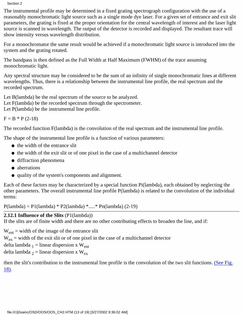
If a light source emits a spectrum which consists of a single monochromatic wavelength lambdao (Fig. 15) and isanalyzed by a perfect spectrometer, the output should be identical to the spectrum of the emission (Fig. 16)which is a perfect line at precisely lambdao.

In reality spectrometers are not perfect and produce an apparent spectral broadening of the purelymonochromatic wavelength. The line profile now has finite width and is known as the "instrumental line profile"(instrumental bandpass). (See Fig. 17).

Section 2


The instrumental profile may be determined in a fixed grating spectrograph configuration with the use of areasonably monochromatic light source such as a single mode dye laser. For a given set of entrance and exit slitparameters, the grating is fixed at the proper orientation for the central wavelength of interest and the laser lightsource is scanned in wavelength. The output of the detector is recorded and displayed. The resultant trace willshow intensity versus wavelength distribution.

For a monochromator the same result would be achieved if a monochromatic light source is introduced into thesystem and the grating rotated.

The bandpass is then defined as the Full Width at Half Maximum (FWHM) of the trace assumingmonochromatic light.

Any spectral structure may be considered to be the sum of an infinity of single monochromatic lines at differentwavelengths. Thus, there is a relationship between the instrumental line profile, the real spectrum and therecorded spectrum.

Let B(lambda) be the real spectrum of the source to be analyzed.Let F(lambda) be the recorded spectrum through the spectrometer.Let P(lambda) be the instrumental line profile.

F = B * P (218)

The recorded function F(lambda) is the convolution of the real spectrum and the instrumental line profile.

The shape of the instrumental line profile is a function of various parameters:

the width of the entrance slit●

the width of the exit slit or of one pixel in the case of a multichannel detector●

diffraction phenomena●

aberrations●

quality of the system's components and alignment.●

Each of these factors may be characterized by a special function Pi(lambda), each obtained by neglecting theother parameters. The overall instrumental line profile P(lambda) is related to the convolution of the individualterms:

P(lambda) = P1(lambda) * P2(lambda) *.....* Pn(lambda) (219)

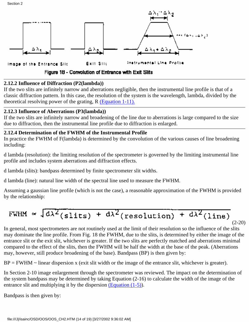
2.12.1 Influence of the Slits (P1(lambda))If the slits are of finite width and there are no other contributing effects to broaden the line, and if:

Went = width of the image of the entrance slitWex = width of the exit slit or of one pixel in the case of a multichannel detectordelta lambda 1 = linear dispersion x Wentdelta lambda 2 = linear dispersion x Wex

then the slit's contribution to the instrumental line profile is the convolution of the two slit functions. (See Fig.18).

Section 2


2.12.2 Influence of Diffraction (P2(lambda))If the two slits are infinitely narrow and aberrations negligible, then the instrumental line profile is that of aclassic diffraction pattern. In this case, the resolution of the system is the wavelength, lambda, divided by thetheoretical resolving power of the grating, R (Equation 111).

2.12.3 Influence of Aberrations (P3(lambda))If the two slits are infinitely narrow and broadening of the line due to aberrations is large compared to the sizedue to diffraction, then the instrumental line profile due to diffraction is enlarged.

2.12.4 Determination of the FWHM of the Instrumental ProfileIn practice the FWHM of F(lambda) is determined by the convolution of the various causes of line broadeningincluding:

d lambda (resolution): the limiting resolution of the spectrometer is governed by the limiting instrumental lineprofile and includes system aberrations and diffraction effects.

d lambda (slits): bandpass determined by finite spectrometer slit widths.

d lambda (line): natural line width of the spectral line used to measure the FWHM.

Assuming a gaussian line profile (which is not the case), a reasonable approximation of the FWHM is providedby the relationship:

(220)In general, most spectrometers are not routinely used at the limit of their resolution so the influence of the slitsmay dominate the line profile. From Fig. 18 the FWHM, due to the slits, is determined by either the image of theentrance slit or the exit slit, whichever is greater. If the two slits are perfectly matched and aberrations minimalcompared to the effect of the slits, then the FWHM will be half the width at the base of the peak. (Aberrationsmay, however, still produce broadening of the base). Bandpass (BP) is then given by:

BP = FWHM ~ linear dispersion x (exit slit width or the image of the entrance slit, whichever is greater).

In Section 2-10 image enlargement through the spectrometer was reviewed. The impact on the determination ofthe system bandpass may be determined by taking Equation (216) to calculate the width of the image of theentrance slit and multiplying it by the dispersion (Equation (15)).

Bandpass is then given by:

Section 2


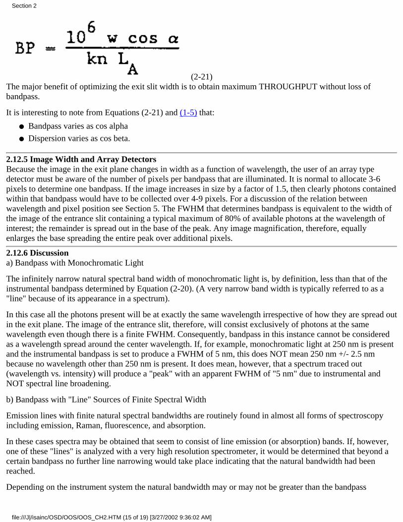
(221)The major benefit of optimizing the exit slit width is to obtain maximum THROUGHPUT without loss ofbandpass.

It is interesting to note from Equations (221) and (15) that:

Bandpass varies as cos alpha●

Dispersion varies as cos beta.●

2.12.5 Image Width and Array DetectorsBecause the image in the exit plane changes in width as a function of wavelength, the user of an array typedetector must be aware of the number of pixels per bandpass that are illuminated. It is normal to allocate 3-6pixels to determine one bandpass. If the image increases in size by a factor of 1.5, then clearly photons containedwithin that bandpass would have to be collected over 4-9 pixels. For a discussion of the relation betweenwavelength and pixel position see Section 5. The FWHM that determines bandpass is equivalent to the width ofthe image of the entrance slit containing a typical maximum of 80% of available photons at the wavelength ofinterest; the remainder is spread out in the base of the peak. Any image magnification, therefore, equallyenlarges the base spreading the entire peak over additional pixels.

2.12.6 Discussiona) Bandpass with Monochromatic Light

The infinitely narrow natural spectral band width of monochromatic light is, by definition, less than that of theinstrumental bandpass determined by Equation (220). (A very narrow band width is typically referred to as a"line" because of its appearance in a spectrum).

In this case all the photons present will be at exactly the same wavelength irrespective of how they are spread outin the exit plane. The image of the entrance slit, therefore, will consist exclusively of photons at the samewavelength even though there is a finite FWHM. Consequently, bandpass in this instance cannot be consideredas a wavelength spread around the center wavelength. If, for example, monochromatic light at 250 nm is presentand the instrumental bandpass is set to produce a FWHM of 5 nm, this does NOT mean 250 nm +/- 2.5 nmbecause no wavelength other than 250 nm is present. It does mean, however, that a spectrum traced out(wavelength vs. intensity) will produce a "peak" with an apparent FWHM of "5 nm" due to instrumental andNOT spectral line broadening.

b) Bandpass with "Line" Sources of Finite Spectral Width

Emission lines with finite natural spectral bandwidths are routinely found in almost all forms of spectroscopyincluding emission, Raman, fluorescence, and absorption.

In these cases spectra may be obtained that seem to consist of line emission (or absorption) bands. If, however,one of these "lines" is analyzed with a very high resolution spectrometer, it would be determined that beyond acertain bandpass no further line narrowing would take place indicating that the natural bandwidth had beenreached.

Depending on the instrument system the natural bandwidth may or may not be greater than the bandpass

Section 2


determined by Equation (220).

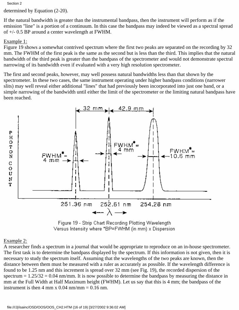
If the natural bandwidth is greater than the instrumental bandpass, then the instrument will perform as if theemission "line" is a portion of a continuum. In this case the bandpass may indeed be viewed as a spectral spreadof +/- 0.5 BP around a center wavelength at FWHM.

Example 1:Figure 19 shows a somewhat contrived spectrum where the first two peaks are separated on the recording by 32mm. The FWHM of the first peak is the same as the second but is less than the third. This implies that the naturalbandwidth of the third peak is greater than the bandpass of the spectrometer and would not demonstrate spectralnarrowing of its bandwidth even if evaluated with a very high resolution spectrometer.

The first and second peaks, however, may well possess natural bandwidths less than that shown by thespectrometer. In these two cases, the same instrument operating under higher bandpass conditions (narrowerslits) may well reveal either additional "lines" that had previously been incorporated into just one band, or asimple narrowing of the bandwidth until either the limit of the spectrometer or the limiting natural bandpass havebeen reached.

Example 2:A researcher finds a spectrum in a journal that would be appropriate to reproduce on an inhouse spectrometer.The first task is to determine the bandpass displayed by the spectrum. If this information is not given, then it isnecessary to study the spectrum itself. Assuming that the wavelengths of the two peaks are known, then thedistance between them must be measured with a ruler as accurately as possible. If the wavelength difference isfound to be 1.25 nm and this increment is spread over 32 mm (see Fig. 19), the recorded dispersion of thespectrum = 1.25/32 = 0.04 nm/mm. It is now possible to determine the bandpass by measuring the distance inmm at the Full Width at Half Maximum height (FWHM). Let us say that this is 4 mm; the bandpass of theinstrument is then 4 mm x 0.04 nm/mm = 0.16 nm.

Section 2


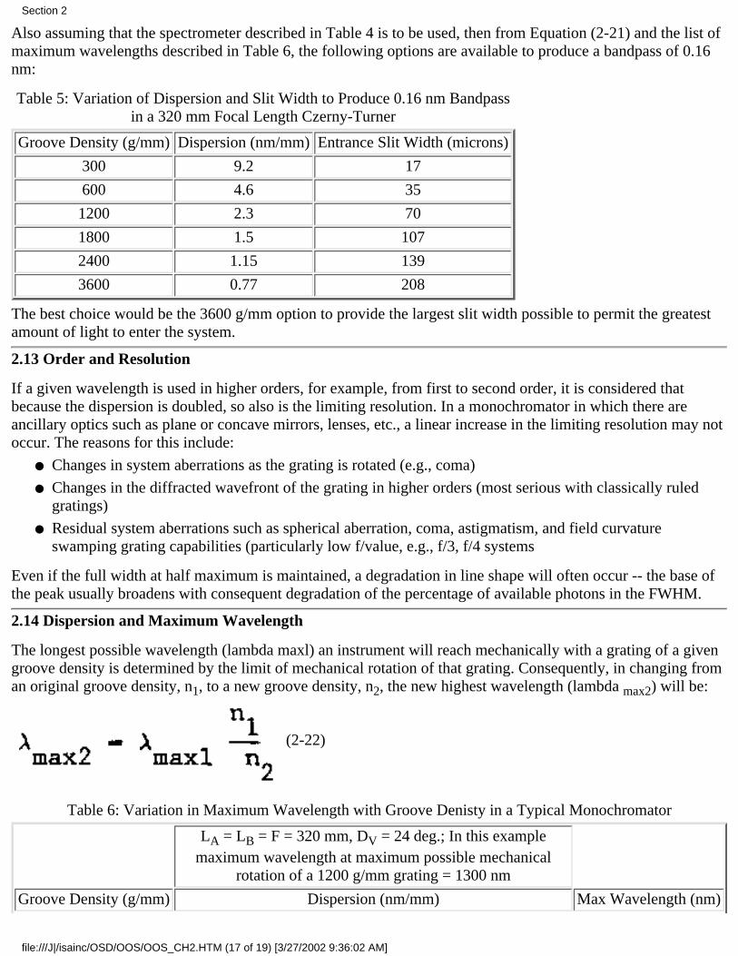
Also assuming that the spectrometer described in Table 4 is to be used, then from Equation (2-21) and the list ofmaximum wavelengths described in Table 6, the following options are available to produce a bandpass of 0.16nm:

Table 5: Variation of Dispersion and Slit Width to Produce 0.16 nm Bandpassin a 320 mm Focal Length Czerny-Turner

Groove Density (g/mm) Dispersion (nm/mm) Entrance Slit Width (microns)

300 9.2 17

600 4.6 35

1200 2.3 70

1800 1.5 107

2400 1.15 139

3600 0.77 208

The best choice would be the 3600 g/mm option to provide the largest slit width possible to permit the greatestamount of light to enter the system.

2.13 Order and Resolution

If a given wavelength is used in higher orders, for example, from first to second order, it is considered thatbecause the dispersion is doubled, so also is the limiting resolution. In a monochromator in which there areancillary optics such as plane or concave mirrors, lenses, etc., a linear increase in the limiting resolution may notoccur. The reasons for this include:

Changes in system aberrations as the grating is rotated (e.g., coma)●

Changes in the diffracted wavefront of the grating in higher orders (most serious with classically ruledgratings)

●

Residual system aberrations such as spherical aberration, coma, astigmatism, and field curvatureswamping grating capabilities (particularly low f/value, e.g., f/3, f/4 systems

●

Even if the full width at half maximum is maintained, a degradation in line shape will often occur -- the base ofthe peak usually broadens with consequent degradation of the percentage of available photons in the FWHM.

2.14 Dispersion and Maximum Wavelength

The longest possible wavelength (lambda maxl) an instrument will reach mechanically with a grating of a givengroove density is determined by the limit of mechanical rotation of that grating. Consequently, in changing froman original groove density, n1, to a new groove density, n2, the new highest wavelength (lambda max2) will be:

(222)

Table 6: Variation in Maximum Wavelength with Groove Denisty in a Typical Monochromator

LA = LB = F = 320 mm, DV = 24 deg.; In this examplemaximum wavelength at maximum possible mechanical

rotation of a 1200 g/mm grating = 1300 nm

Groove Density (g/mm) Dispersion (nm/mm) Max Wavelength (nm)

Section 2


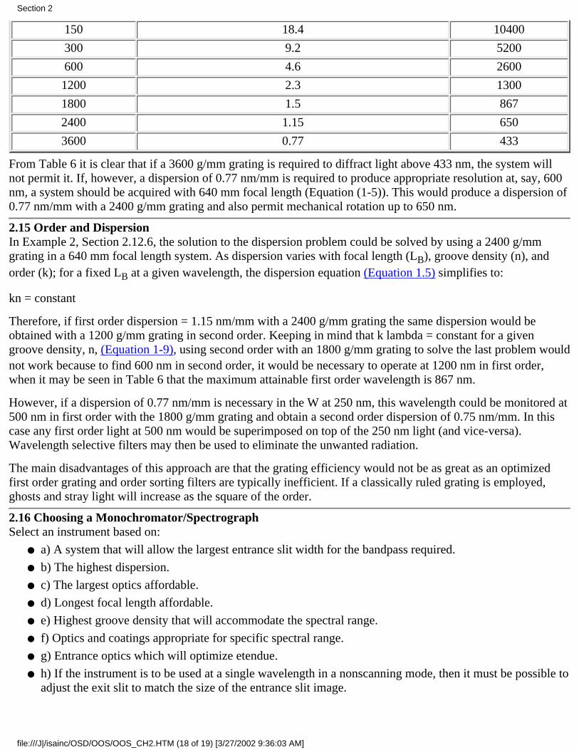
150 18.4 10400

300 9.2 5200

600 4.6 2600

1200 2.3 1300

1800 1.5 867

2400 1.15 650

3600 0.77 433

From Table 6 it is clear that if a 3600 g/mm grating is required to diffract light above 433 nm, the system willnot permit it. If, however, a dispersion of 0.77 nm/mm is required to produce appropriate resolution at, say, 600nm, a system should be acquired with 640 mm focal length (Equation (15)). This would produce a dispersion of0.77 nm/mm with a 2400 g/mm grating and also permit mechanical rotation up to 650 nm.

2.15 Order and DispersionIn Example 2, Section 2.12.6, the solution to the dispersion problem could be solved by using a 2400 g/mmgrating in a 640 mm focal length system. As dispersion varies with focal length (LB), groove density (n), andorder (k); for a fixed LB at a given wavelength, the dispersion equation (Equation 1.5) simplifies to:

kn = constant

Therefore, if first order dispersion = 1.15 nm/mm with a 2400 g/mm grating the same dispersion would beobtained with a 1200 g/mm grating in second order. Keeping in mind that k lambda = constant for a givengroove density, n, (Equation 19), using second order with an 1800 g/mm grating to solve the last problem wouldnot work because to find 600 nm in second order, it would be necessary to operate at 1200 nm in first order,when it may be seen in Table 6 that the maximum attainable first order wavelength is 867 nm.

However, if a dispersion of 0.77 nm/mm is necessary in the W at 250 nm, this wavelength could be monitored at500 nm in first order with the 1800 g/mm grating and obtain a second order dispersion of 0.75 nm/mm. In thiscase any first order light at 500 nm would be superimposed on top of the 250 nm light (and vice-versa).Wavelength selective filters may then be used to eliminate the unwanted radiation.

The main disadvantages of this approach are that the grating efficiency would not be as great as an optimizedfirst order grating and order sorting filters are typically inefficient. If a classically ruled grating is employed,ghosts and stray light will increase as the square of the order.

2.16 Choosing a Monochromator/SpectrographSelect an instrument based on:

a) A system that will allow the largest entrance slit width for the bandpass required.●

b) The highest dispersion.●

c) The largest optics affordable.●

d) Longest focal length affordable.●

e) Highest groove density that will accommodate the spectral range.●

f) Optics and coatings appropriate for specific spectral range.●

g) Entrance optics which will optimize etendue.●

h) If the instrument is to be used at a single wavelength in a nonscanning mode, then it must be possible toadjust the exit slit to match the size of the entrance slit image.

●

Section 2


Remember: f/value is not always the controlling factor of throughput. For example, light may be collected from asource at f/1 and projected onto the entrance slit of an f/6 monochromator so that the entire image is containedwithin the slit. Then the system will operate on the basis of the photon collection in the f/l cone and not the f/6cone of the monochromator. See Section 3.

[Go to Section 3] [Return to Table of Contents] [Back to Section 1]

Section 2


Section 3: Spectrometer Throughput andEtendue

3.1 DefinitionsFlux In the spectrometer system flux is given by energy/time (photons/sec, or watts), emitted from a lightsource or slit of given area, into a solid angle (Q) at a given wavelength (or bandpass).

Intensity (I) The distribution of flux at a given wavelength (or bandpass) per solid angle (watts/steradian).

Radiance (Luminance) (B) The intensity when spread over a given surface. Also defined as B =Intensity/Surface Area of the Source (watts/steradian/cm2).

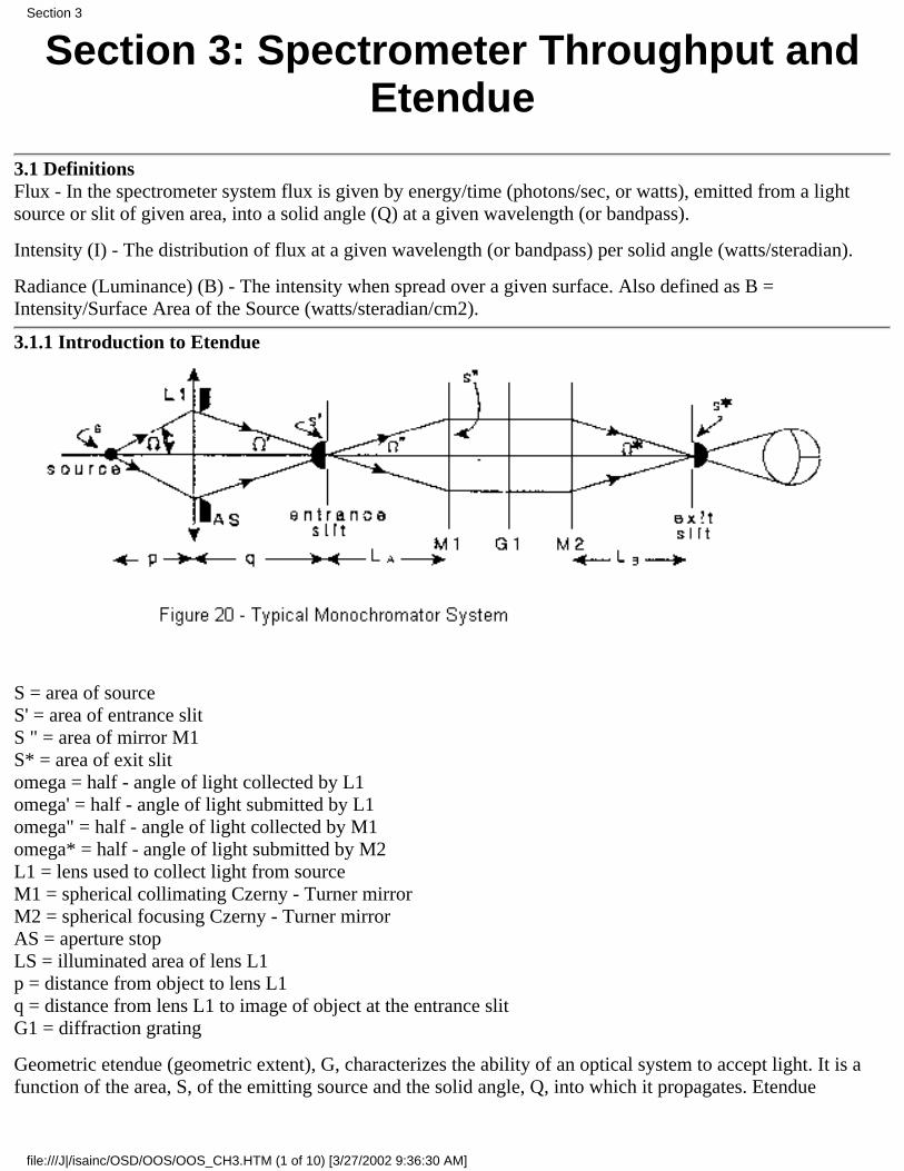
3.1.1 Introduction to Etendue

S = area of sourceS' = area of entrance slitS " = area of mirror M1S* = area of exit slitomega = half angle of light collected by L1omega' = half angle of light submitted by L1omega" = half angle of light collected by M1omega* = half angle of light submitted by M2L1 = lens used to collect light from sourceM1 = spherical collimating Czerny Turner mirrorM2 = spherical focusing Czerny Turner mirrorAS = aperture stopLS = illuminated area of lens L1p = distance from object to lens L1q = distance from lens L1 to image of object at the entrance slitG1 = diffraction grating

Geometric etendue (geometric extent), G, characterizes the ability of an optical system to accept light. It is afunction of the area, S, of the emitting source and the solid angle, Q, into which it propagates. Etendue

Section 3


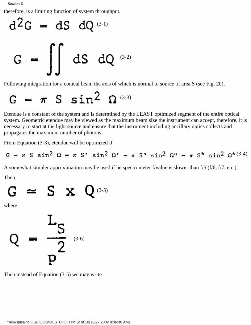
therefore, is a limiting function of system throughput.

(31)

(32)

Following integration for a conical beam the axis of which is normal to source of area S (see Fig. 20),

(33)

Etendue is a constant of the system and is determined by the LEAST optimized segment of the entire opticalsystem. Geometric etendue may be viewed as the maximum beam size the instrument can accept, therefore, it isnecessary to start at the light source and ensure that the instrument including ancillary optics collects andpropagates the maximum number of photons.

From Equation (33), etendue will be optimized if

(34)

A somewhat simpler approximation may be used if he spectrometer f/value is slower than f/5 (f/6, f/7, etc.).

Then,

(35)

where

(36)

Then instead of Equation (35) we may write

Section 3


etc. (37)

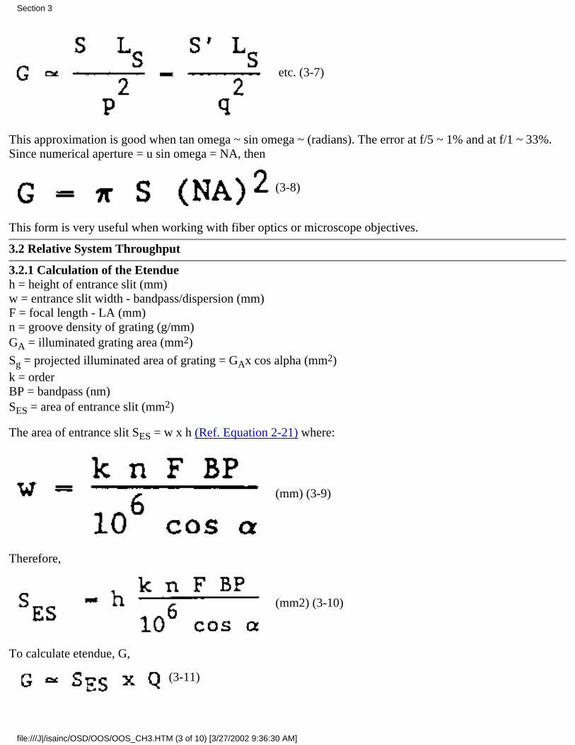
This approximation is good when tan omega ~ sin omega ~ (radians). The error at f/5 ~ 1% and at f/1 ~ 33%.Since numerical aperture = u sin omega = NA, then

(38)

This form is very useful when working with fiber optics or microscope objectives.

3.2 Relative System Throughput

3.2.1 Calculation of the Etendueh = height of entrance slit (mm)w = entrance slit width bandpass/dispersion (mm)F = focal length LA (mm)n = groove density of grating (g/mm)GA = illuminated grating area (mm2)

Sg = projected illuminated area of grating = GAx cos alpha (mm2)k = orderBP = bandpass (nm)SES = area of entrance slit (mm2)

The area of entrance slit SES = w x h (Ref. Equation 2-21) where:

(mm) (39)

Therefore,

(mm2) (310)

To calculate etendue, G,

(311)

Section 3


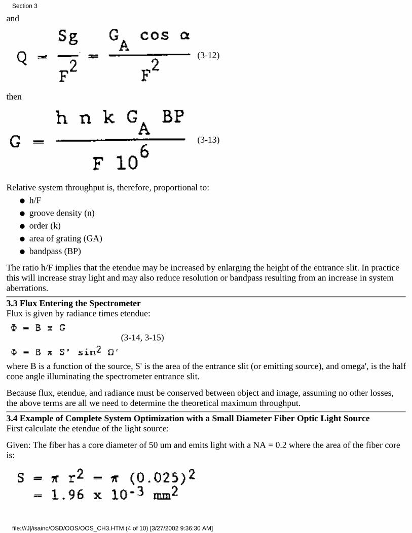
and

(312)

then

(313)

Relative system throughput is, therefore, proportional to:

h/F●

groove density (n)●

order (k)●

area of grating (GA)●

bandpass (BP)●

The ratio h/F implies that the etendue may be increased by enlarging the height of the entrance slit. In practicethis will increase stray light and may also reduce resolution or bandpass resulting from an increase in systemaberrations.

3.3 Flux Entering the SpectrometerFlux is given by radiance times etendue:

(3-14, 3-15)

where B is a function of the source, S' is the area of the entrance slit (or emitting source), and omega', is the halfcone angle illuminating the spectrometer entrance slit.

Because flux, etendue, and radiance must be conserved between object and image, assuming no other losses,the above terms are all we need to determine the theoretical maximum throughput.

3.4 Example of Complete System Optimization with a Small Diameter Fiber Optic Light SourceFirst calculate the etendue of the light source:

Given: The fiber has a core diameter of 50 um and emits light with a NA = 0.2 where the area of the fiber coreis:

Section 3


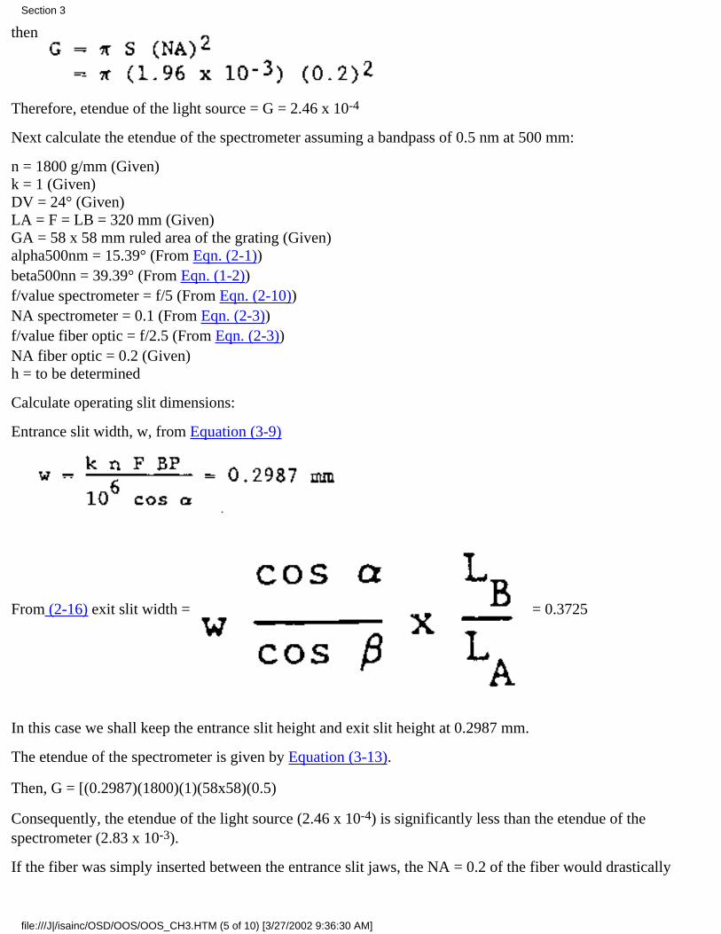
then

Therefore, etendue of the light source = G = 2.46 x 104

Next calculate the etendue of the spectrometer assuming a bandpass of 0.5 nm at 500 mm:

n = 1800 g/mm (Given)k = 1 (Given)DV = 24° (Given)LA = F = LB = 320 mm (Given)GA = 58 x 58 mm ruled area of the grating (Given)alpha500nm = 15.39° (From Eqn. (21))beta500nn = 39.39° (From Eqn. (12))f/value spectrometer = f/5 (From Eqn. (210))NA spectrometer = 0.1 (From Eqn. (23))f/value fiber optic = f/2.5 (From Eqn. (23))NA fiber optic = 0.2 (Given)h = to be determined

Calculate operating slit dimensions:

Entrance slit width, w, from Equation (39)

From (216) exit slit width = = 0.3725

In this case we shall keep the entrance slit height and exit slit height at 0.2987 mm.

The etendue of the spectrometer is given by Equation (313).

Then, G = [(0.2987)(1800)(1)(58x58)(0.5)

Consequently, the etendue of the light source (2.46 x 104) is significantly less than the etendue of thespectrometer (2.83 x 103).

If the fiber was simply inserted between the entrance slit jaws, the NA = 0.2 of the fiber would drastically

Section 3


overfill the NA = 0.1 of the spectrometer (f/2.5 to f/5) both losing photons and creating stray light. In this casethe SYSTEM etendue would be determined by the area of the fiber's core and the NA of the spectrometer.

The point now is to reimage the light emanating from the fiber in such a way that the etendue of the fiber isbrought up to that of the spectrometer thereby permitting total capture and propagation of all available photons.

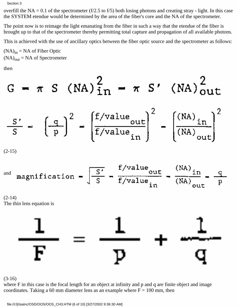
This is achieved with the use of ancillary optics between the fiber optic source and the spectrometer as follows:

(NA)in = NA of Fiber Optic(NA)out = NA of Spectrometer

then

(2-15)

and

(2-14)The thin lens equation is

(3-16)where F in this case is the focal length for an object at infinity and p and q are finite object and imagecoordinates. Taking a 60 mm diameter lens as an example where F = 100 mm, then

Section 3


magnification = NAin / NAout = q / p = 0.2 / 0.2 = 2

Substituting in Equation (316)

1 / 100 = 1 / p + 1 /2p

After solving, p = 150 mm and q = 300 mm but

f/valueout = 1 / 2(NA)out = q / d

then = 300 x 0.2 = 60 mm.

f/valuein = 1 / 2(NA)in = q / d

then d = 150 x 0.4 = 60 mm.

Therefore, the light from the fiber is collected by a lens with a 150 mm object distance, p, and projects animage of the fiber core on the spectrometer entrance slit 300 mm, q, from the lens. The f/values are matched toboth the light propagating from the fiber and to that of the spectrometer. The image, however, is magnified by afactor of 2.

Considering that we require an entrance slit width of 0.2987 mm to produce a bandpass of 0.5 nm, the resultingimage of 100 u (2 x 50 u core diam ) underfills the slit, thereby ensuring that all the light collected willpropagate through the system. As a matter of interest, because the image of the fiber core has a width less thanthe slit jaws, the bandpass will be determined by the image of the core itself. Stray light will be lessened byreducing the slit jaws to perfectly contain the core's image (see Section 4).

3.5 Example of Complete System Optimization with an Extended Light SourceAn "extended light source" is one where the source itself is considerably larger than the slit width necessary toproduce an appropriate bandpass. In this case the etendue of the spectrometer will be less than that of the lightsource.

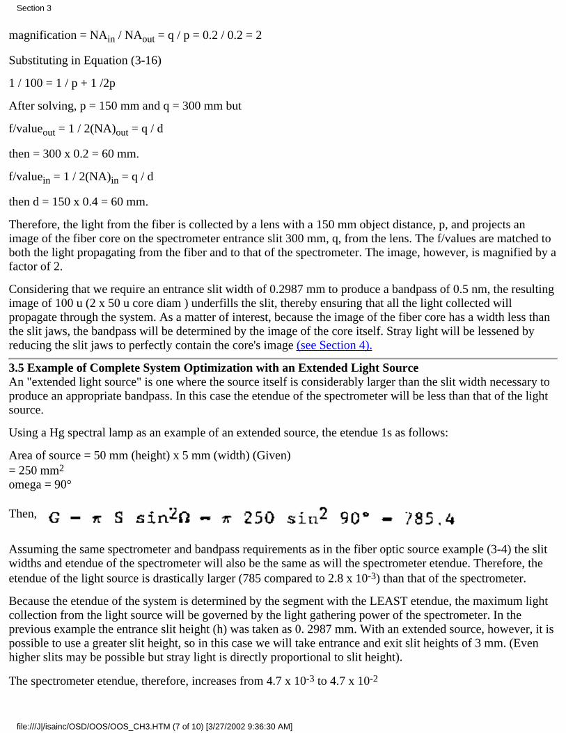
Using a Hg spectral lamp as an example of an extended source, the etendue 1s as follows:

Area of source = 50 mm (height) x 5 mm (width) (Given)= 250 mm2

omega = 90°

Then,

Assuming the same spectrometer and bandpass requirements as in the fiber optic source example (34) the slitwidths and etendue of the spectrometer will also be the same as will the spectrometer etendue. Therefore, theetendue of the light source is drastically larger (785 compared to 2.8 x 103) than that of the spectrometer.

Because the etendue of the system is determined by the segment with the LEAST etendue, the maximum lightcollection from the light source will be governed by the light gathering power of the spectrometer. In theprevious example the entrance slit height (h) was taken as 0. 2987 mm. With an extended source, however, it ispossible to use a greater slit height, so in this case we will take entrance and exit slit heights of 3 mm. (Evenhigher slits may be possible but stray light is directly proportional to slit height).

The spectrometer etendue, therefore, increases from 4.7 x 103 to 4.7 x 102

Section 3


This then will be the effective etendue of the system and will govern the light source. The best way toaccommodate this is to sample an area of the of the Hg lamp equivalent to the entrance slit area and image itonto the entrance slit with the same solid angle as that determined by the diffraction grating (Equation (312) ).

To determine the geometric configuration of the entrance optics take the same 60 mm diameter lens (L1) with a100 mm focal length as that used in the previous example.

We know that the entrance slit dimensions determine the area of the source to be sampled, therefore, SES = areaof the source S.

The source should be imaged 1:1 onto the entrance slit, therefore, magnification = 1.

Taking the thin lens equation

1 / F = 1 / p + 1 / q where q / p = 1

p = 2F and q = 2F

The Hg lamp should be placed 200 mm away from lens L1 which in turn should he 200 mm from the entranceslit.

The diameter required to produce the correct f/value is then determined by the spectrometer whose f/value = 5.

Therefore d = 200 / 5 = 40 mm

The 60 mm lens should, therefore, be aperture stopped down to 40 mm to permit the correct solid angle to enterthe spectrometer.

This system will now achieve maximum light collection.

3.6 Variation of Throughput and Bandpass with Slit WidthsAssume: The image of the source overfills the entrance slit.

wi = original entrance slit width (e.g., 100 um)

wo = exit slit width (original width of entrance slit image, e.g., 110 um)

3.6.1 Continuous Spectral SourceFor example, a tungsten halogen lamp or a spectrum where line widths are significantly greater thaninstrumental bandpass. (This is often the case in fluorescence experiments.)

Throughput will vary as a function of the product of change in bandpass and change in etendue.

Case 1: Double the entrance slit width, wi, but keep exit slit unchanged, therefore,

entrance slit = 2wi ( 200 um)exit slit = wo (110 um)

Etendue remains the same (determined by exit slit).Bandpass is doubled.Throughput is doubled.

Case 2: Double the exit slit width, wo, but keep entrance slit unchanged, therefore.

entrance slit = wi (100 um)

Section 3


exit slit = 2wo ( 220 um)

Etendue remains the same (determined by entrance slit).Bandpass is doubled.Throughput is doubled.

Note: Doubling the exit slit allows a broader segment of the spectrum through the exit and, therefore, increasesthe photon flux.

Case 3: Double both the entrance and exit slit widths, therefore,

entrance slit = 2wi (200 um)exit slit = 2wo (220 um)

Etendue is doubled.Bandpass is doubled.Throughput is quadrupled.

3.6.2 Discrete Spectral SourceA light source that will produce a number of monochromatic wavelengths is called a discrete spectral source.

In practice an apparently monochromatic line source is often a discrete segment of a continuum. It is assumedthat the natural line width is less than the minimum achievable bandpass of the instrument.

Throughput will then vary as a function of change in etendue and is independent of bandpass.

Case 1: Double the entrance slit width, wi, but keep exit slit unchanged, therefore,

entrance slit = 2wi (200 um)exit slit = wo (110 um)

Etendue remains the same (determined by exit slit)Bandpass is doubled.Throughput remains the same.

Case 2: Double the exit slit width, wo, but keep entrance slit unchanged therefore.

entrance slit = wi (100 um)exit slit = wo (220 um)

Etendue remains the same (determined by entrance slit).Bandpass is doubled.Throughput remains the same.

Note: For a discrete spectral source, doubling the exit slit width will not cause a change in the throughputbecause it does not allow an increase of photon flux for the instrument.

Case 3: Double both the entrance and exit slit widths, therefore,

entrance slit = 2wi (200 um)exit slit = 2wo (220 um)

Etendue is doubled.

Section 3


Bandpass is doubled.Throughput is doubled.


Section 3


4 Optical Signal-to-Noise Ratio and StrayLight

Stray light and the effect it has on Optical Signal to Noise ratio (S/N) falls into one of two majorcategories either a) random scatter from mirrors, gratings, etc. or b) directional stray light such asreflections, re entry spectra, grating ghosts and grating generated focused stray light.

4.1 Random Stray LightConsider first how much light there is to begin with at the primary wavelength of interest then compare itto other wavelengths that may be present as scatter.

4.1.1 Optical Signal to Noise Ratio in a SpectrometerTo determine the ratio of signal to noise each of the components must first be quantified.

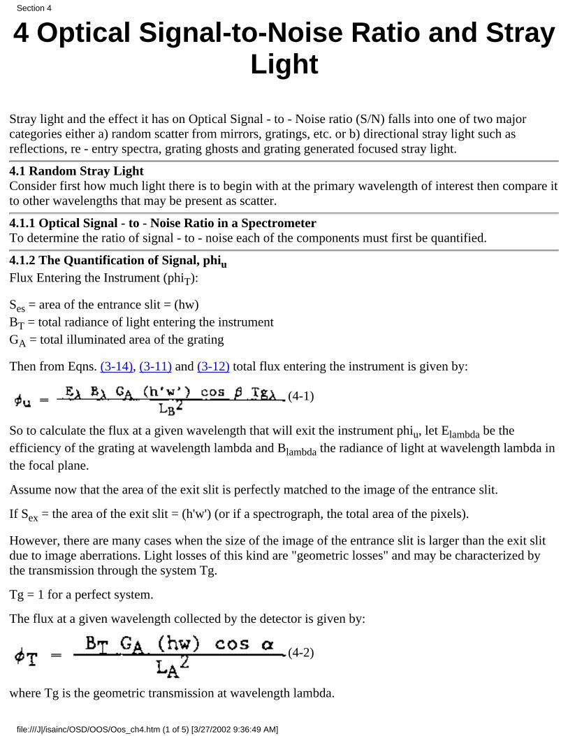
4.1.2 The Quantification of Signal, phiuFlux Entering the Instrument (phiT):

Ses = area of the entrance slit = (hw)BT = total radiance of light entering the instrumentGA = total illuminated area of the grating

Then from Eqns. (314), (311) and (312) total flux entering the instrument is given by:

(4-1)

So to calculate the flux at a given wavelength that will exit the instrument phiu, let Elambda be theefficiency of the grating at wavelength lambda and Blambda the radiance of light at wavelength lambda inthe focal plane.

Assume now that the area of the exit slit is perfectly matched to the image of the entrance slit.

If Sex = the area of the exit slit = (h'w') (or if a spectrograph, the total area of the pixels).

However, there are many cases when the size of the image of the entrance slit is larger than the exit slitdue to image aberrations. Light losses of this kind are "geometric losses" and may be characterized bythe transmission through the system Tg.

Tg = 1 for a perfect system.

The flux at a given wavelength collected by the detector is given by:

(42)

where Tg is the geometric transmission at wavelength lambda.

Section 4


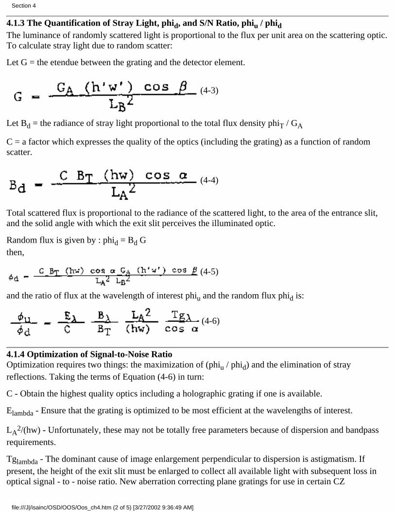
4.1.3 The Quantification of Stray Light, phid, and S/N Ratio, phiu / phidThe luminance of randomly scattered light is proportional to the flux per unit area on the scattering optic.To calculate stray light due to random scatter:

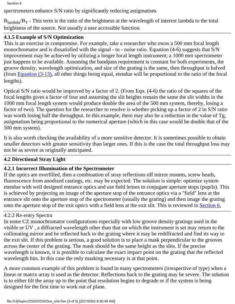
Let G = the etendue between the grating and the detector element.

(43)

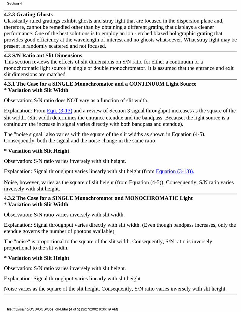
Let Bd = the radiance of stray light proportional to the total flux density phiT / GA

C = a factor which expresses the quality of the optics (including the grating) as a function of randomscatter.

(4-4)

Total scattered flux is proportional to the radiance of the scattered light, to the area of the entrance slit,and the solid angle with which the exit slit perceives the illuminated optic.

Random flux is given by : phid = Bd Gthen,

(4-5)

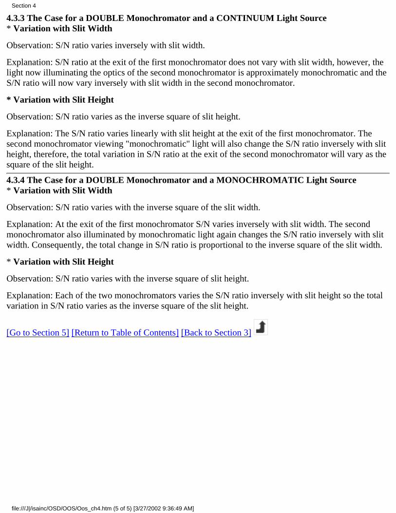
and the ratio of flux at the wavelength of interest phiu and the random flux phid is:

(4-6)

4.1.4 Optimization of SignaltoNoise RatioOptimization requires two things: the maximization of (phiu / phid) and the elimination of strayreflections. Taking the terms of Equation (46) in turn:

C Obtain the highest quality optics including a holographic grating if one is available.

Elambda Ensure that the grating is optimized to be most efficient at the wavelengths of interest.

LA2/(hw) Unfortunately, these may not be totally free parameters because of dispersion and bandpass

requirements.

Tglambda The dominant cause of image enlargement perpendicular to dispersion is astigmatism. Ifpresent, the height of the exit slit must be enlarged to collect all available light with subsequent loss inoptical signal to noise ratio. New aberration correcting plane gratings for use in certain CZ

Section 4


spectrometers enhance S/N ratio by significantly reducing astigmatism.

Blambda/BT This term is the ratio of the brightness at the wavelength of interest lambda to the totalbrightness of the source. Not usually a user accessible function.

4.1.5 Example of S/N OptimizationThis is an exercise in compromise. For example, take a researcher who owns a 500 mm focal lengthmonochromator and is dissatisfied with the signal to - noise ratio. Equation (46) suggests that S/Nimprovement may be achieved by utilizing a longer focal length instrument; a 1000 mm spectrometerjust happens to be available. Assuming the bandpass requirement is constant for both experiments, thegroove density, wavelength optimization, and size of the grating is the same, then throughput is halved(from Equation (313), all other things being equal, etendue will be proportional to the ratio of the focallengths).

Optical S/N ratio would be improved by a factor of 2. (From Eqn. (46) the ratio of the squares of thefocal lengths gives a factor of four and assuming the slit heights remain the same the slit widths in the1000 mm focal length system would produce double the area of the 500 mm system, thereby, losing afactor of two). The question for the researcher to resolve is whether picking up a factor of 2 in S/N ratiowas worth losing half the throughput. In this example, there may also be a reduction in the value of Tg,astigmatism being proportional to the numerical aperture (which in this case would be double that of the500 mm system).

It is also worth checking the availability of a more sensitive detector. It is sometimes possible to obtainsmaller detectors with greater sensitivity than larger ones. If this is the case the total throughput loss maynot be as severe as originally anticipated.

4.2 Directional Stray Light

4.2.1 Incorrect Illumination of the SpectrometerIf the optics are overfilled, then a combination of stray reflections off mirror mounts, screw heads,fluorescence from anodized castings, etc. may be expected. The solution is simple: optimize systemetendue with well designed entrance optics and use field lenses to conjugate aperture stops (pupils). Thisis achieved by projecting an image of the aperture stop of the entrance optics via a "field" lens at theentrance slit onto the aperture stop of the spectrometer (usually the grating) and then image the gratingonto the aperture stop of the exit optics with a field lens at the exit slit. This is reviewed in Section 6.

4.2.2 Reentry SpectraIn some CZ monochromator configurations especially with low groove density gratings used in thevisible or UV , a diffracted wavelength other than that on which the instrument is set may return to thecollimating mirror and be reflected back to the grating where it may be rediffracted and find its way tothe exit slit. If this problem is serious, a good solution is to place a mask perpendicular to the groovesacross the center of the grating. The mask should be the same height as the slits. If the precisewavelength is known, it is possible to calculate the exact impact point on the grating that the reflectedwavelength hits. In this case the only masking necessary is at that point.

A more common example of this problem is found in many spectrometers (irrespective of type) when alinear or matrix array is used as the detector. Reflections back to the grating may be severe. The solutionis to either tilt the array up to the point that resolution begins to degrade or if the system is beingdesigned for the first time to work out of plane.

Section 4


4.2.3 Grating GhostsClassically ruled gratings exhibit ghosts and stray light that are focused in the dispersion plane and,therefore, cannot be remedied other than by obtaining a different grating that displays a cleanerperformance. One of the best solutions is to employ an ion etched blazed holographic grating thatprovides good efficiency at the wavelength of interest and no ghosts whatsoever. What stray light may bepresent is randomly scattered and not focused.

4.3 S/N Ratio ant Slit DimensionsThis section reviews the effects of slit dimensions on S/N ratio for either a continuum or amonochromatic light source in single or double monochromator. It is assumed that the entrance and exitslit dimensions are matched.

4.3.1 The Case for a SINGLE Monochromator and a CONTINUUM Light Source* Variation with Slit Width

Observation: S/N ratio does NOT vary as a function of slit width.

Explanation: From Eqn. (313) and a review of Section 3 signal throughput increases as the square of theslit width. (Slit width determines the entrance etendue and the bandpass. Because, the light source is acontinuum the increase in signal varies directly with both bandpass and etendue).

The "noise signal" also varies with the square of the slit widths as shown in Equation (45).Consequently, both the signal and the noise change in the same ratio.

* Variation with Slit Height

Observation: S/N ratio varies inversely with slit height.

Explanation: Signal throughput varies linearly with slit height (from Equation (313)).

Noise, however, varies as the square of slit height (from Equation (45)). Consequently, S/N ratio variesinversely with slit height.

4.3.2 The Case for a SINGLE Monochromator and MONOCHROMATIC Light* Variation with Slit Width

Observation: S/N ratio varies inversely with slit width.

Explanation: Signal throughput varies directly with slit width. (Even though bandpass increases, only theetendue governs the number of photons available).

The "noise" is proportional to the square of the slit width. Consequently, S/N ratio is inverselyproportional to the slit width.


Observation: S/N ratio varies inversely with slit height.

Explanation: Signal throughput varies linearly with slit height.

Noise varies as the square of the slit height. Consequently, S/N ratio varies inversely with slit height.

Section 4


4.3.3 The Case for a DOUBLE Monochromator and a CONTINUUM Light Source* Variation with Slit Width

Observation: S/N ratio varies inversely with slit width.

Explanation: S/N ratio at the exit of the first monochromator does not vary with slit width, however, thelight now illuminating the optics of the second monochromator is approximately monochromatic and theS/N ratio will now vary inversely with slit width in the second monochromator.


Observation: S/N ratio varies as the inverse square of slit height.

Explanation: The S/N ratio varies linearly with slit height at the exit of the first monochromator. Thesecond monochromator viewing "monochromatic" light will also change the S/N ratio inversely with slitheight, therefore, the total variation in S/N ratio at the exit of the second monochromator will vary as thesquare of the slit height.

4.3.4 The Case for a DOUBLE Monochromator and a MONOCHROMATIC Light Source* Variation with Slit Width

Observation: S/N ratio varies with the inverse square of the slit width.

Explanation: At the exit of the first monochromator S/N varies inversely with slit width. The secondmonochromator also illuminated by monochromatic light again changes the S/N ratio inversely with slitwidth. Consequently, the total change in S/N ratio is proportional to the inverse square of the slit width.


Observation: S/N ratio varies with the inverse square of slit height.

Explanation: Each of the two monochromators varies the S/N ratio inversely with slit height so the totalvariation in S/N ratio varies as the inverse square of the slit height.


Section 4


5 The Relationship Between Wavelengthand Pixel Position on an Array

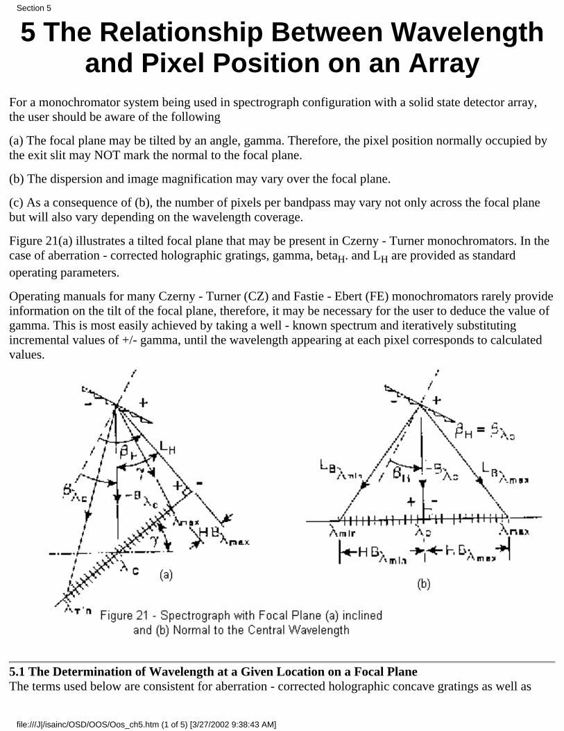
For a monochromator system being used in spectrograph configuration with a solid state detector array,the user should be aware of the following

(a) The focal plane may be tilted by an angle, gamma. Therefore, the pixel position normally occupied bythe exit slit may NOT mark the normal to the focal plane.

(b) The dispersion and image magnification may vary over the focal plane.

(c) As a consequence of (b), the number of pixels per bandpass may vary not only across the focal planebut will also vary depending on the wavelength coverage.

Figure 21(a) illustrates a tilted focal plane that may be present in Czerny - Turner monochromators. In thecase of aberration corrected holographic gratings, gamma, betaH. and LH are provided as standardoperating parameters.

Operating manuals for many Czerny Turner (CZ) and Fastie Ebert (FE) monochromators rarely provideinformation on the tilt of the focal plane, therefore, it may be necessary for the user to deduce the value ofgamma. This is most easily achieved by taking a well known spectrum and iteratively substitutingincremental values of +/- gamma, until the wavelength appearing at each pixel corresponds to calculatedvalues.

5.1 The Determination of Wavelength at a Given Location on a Focal PlaneThe terms used below are consistent for aberration corrected holographic concave gratings as well as

Section 5


Czerny Turner and Fastie Ebert spectrometers.

Lambda C - Wavelength (in nm) at center of array (where exit slit would usually be located)LA - Entrance arm length (mm)L B lambda n - Exit arm length to each wavelength located on the focal plane (mm)L B lambda c - Exit arm length to lambda c (Czerny Turner and Fastie Ebert monochromators LA = L Blambda c =F)LH - Perpendicular distance from grating or focusing mirror to the focal plane (mm)F - Instrument "focal length". For CZ and FE monochromators LA = F = LB. (mm)beta H - Angle from LH to the normal to the grating (this will vary in a scanning instrument)beta lambda n - Angle of diffraction at wavelength nbeta lambda c - Angle of diffraction at center wavelengthH B lambda n - Distance from the intercept of the normal to the focal plane to the wavelength lambda nH B lambda c - Distance from the intercept of the normal to the focal plane to the wavelength lambda cPmin - Pixel # at extremity corresponding to lambda min (e.g., # 1)Pmax - Pixel # at extremity corresponding to lambda max (e.g., # 1024)Pw - Pixel width (mm)Pc - Pixel # at lambda c (e.g., # 512)P lambda - Pixel # at lambda nInclination of the focal plane measured at the location normally occupied by the exit slit, lambda c. (This isusually the center of the array. However, provided that the pixel marking this location is known, the arraymay be placed as the user finds most useful). For this reason, it is very convenient to use a spectrometerthat permits simple interchange from scanning to spectrograph by means of a swing away mirror. Theinstrument may then be set up with a standard slit using, for example, a mercury lamp. Switching tospectrograph mode enables identification of the pixel, Pc, illuminated by the wavelength previously at theexit slit.

The equations that follow are for Czerny Turner type instruments where gamma = 0° in one case andgamma does not equal 0 in the other.

Case 1 gamma = 0°.

See Figure 21(b).

LH = LB = F at lambda c (mm)beta H = beta at lambda cHB lambda n = Pw (P lambda - Pc) (mm)

HB is negative for wavelengths shorter than lambda c.HB is positive for wavelengths longer than lambda c.

beta lambda n = betaH tan-1 (HB lambda n /LH) (5l)

Note: The secret of success (and reason for failure) is frequently the level of understanding of the signconvention. Be consistent, make reasonably accurate sketches whenever possible and be philosophical

Section 5


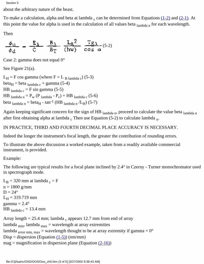
about the arbitrary nature of the beast.

To make a calculation, alpha and beta at lambda c can be determined from Equations (12) and (21). Atthis point the value for alpha is used in the calculation of all values beta lambda n for each wavelength.

Then

(52)

Case 2: gamma does not equal 0°

See Figure 21(a).

LH = F cos gamma (where F = L B lambda c) (5-3)betaH = beta lambda c + gamma (54)HB lambda c = F sin gamma (55)HB lambda n = Pw (P lambda Pc) + HB lambda c (56)

beta lambda n = betaH tan-1 (HB lambda n /LH) (57)

Again keeping significant concern for the sign of HB lambda n, proceed to calculate the value beta lambda nafter first obtaining alpha at lambda c Then use Equation (52) to calculate lambda n.

IN PRACTICE, THIRD AND FOURTH DECIMAL PLACE ACCURACY IS NECESSARY.

Indeed the longer the instrument's focal length, the greater the contribution of rounding errors.

To illustrate the above discussion a worked example, taken from a readily available commercialinstrument, is provided.

Example:

The following are typical results for a focal plane inclined by 2.4° in Czerny Turner monochromator usedin spectrograph mode.

LB = 320 mm at lambda c = Fn = 1800 g/mmD = 24°LH = 319.719 mmgamma = 2.4°HB lambda c = 13.4 mm

Array length = 25.4 mm; lambda c appears 12.7 mm from end of arraylambda min, lambda max = wavelength at array extremitieslambda error min, max = wavelength thought to be at array extremity if gamma = 0°Disp = dispersion (Equation (15)) (nm/mm)mag = magnification in dispersion plane (Equation (216))

Section 5


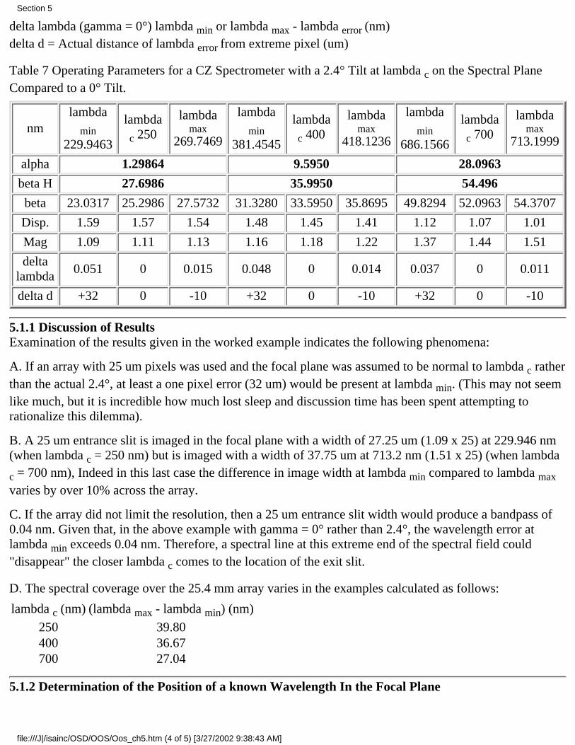
delta lambda (gamma = 0°) lambda min or lambda max - lambda error (nm)delta d = Actual distance of lambda error from extreme pixel (um)

Table 7 Operating Parameters for a CZ Spectrometer with a 2.4° Tilt at lambda c on the Spectral PlaneCompared to a 0° Tilt.

nmlambda

min229.9463

lambdac 250

lambdamax

269.7469

lambdamin

381.4545

lambdac 400

lambdamax

418.1236

lambdamin

686.1566

lambdac 700

lambdamax

713.1999

alpha 1.29864 9.5950 28.0963

beta H 27.6986 35.9950 54.496

beta 23.0317 25.2986 27.5732 31.3280 33.5950 35.8695 49.8294 52.0963 54.3707

Disp. 1.59 1.57 1.54 1.48 1.45 1.41 1.12 1.07 1.01

Mag 1.09 1.11 1.13 1.16 1.18 1.22 1.37 1.44 1.51

deltalambda

0.051 0 0.015 0.048 0 0.014 0.037 0 0.011

delta d +32 0 -10 +32 0 -10 +32 0 -10

5.1.1 Discussion of ResultsExamination of the results given in the worked example indicates the following phenomena:

A. If an array with 25 um pixels was used and the focal plane was assumed to be normal to lambda c ratherthan the actual 2.4°, at least a one pixel error (32 um) would be present at lambda min. (This may not seemlike much, but it is incredible how much lost sleep and discussion time has been spent attempting torationalize this dilemma).

B. A 25 um entrance slit is imaged in the focal plane with a width of 27.25 um (1.09 x 25) at 229.946 nm(when lambda c = 250 nm) but is imaged with a width of 37.75 um at 713.2 nm (1.51 x 25) (when lambda

c = 700 nm), Indeed in this last case the difference in image width at lambda min compared to lambda maxvaries by over 10% across the array.

C. If the array did not limit the resolution, then a 25 um entrance slit width would produce a bandpass of0.04 nm. Given that, in the above example with gamma = 0° rather than 2.4°, the wavelength error atlambda min exceeds 0.04 nm. Therefore, a spectral line at this extreme end of the spectral field could"disappear" the closer lambda c comes to the location of the exit slit.

D. The spectral coverage over the 25.4 mm array varies in the examples calculated as follows:

lambda c (nm) (lambda max - lambda min) (nm)

250 39.80400 36.67700 27.04

5.1.2 Determination of the Position of a known Wavelength In the Focal Plane

Section 5


In this case, provided lambda c is known, alpha, betaH, and LH may be determined as above. If lambda n isknown, the beta lambda n may be obtained from the Grating Equation (11). Then

HB lambda n = LH tan (betaH - beta lambda n) (58)

This formula is most useful for constructing alignment targets with the location of known spectral linesmarked on a screen or etched into a ribbon, etc.


Section 5


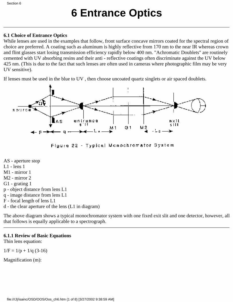
6 Entrance Optics

6.1 Choice of Entrance OpticsWhile lenses are used in the examples that follow, front surface concave mirrors coated for the spectral region ofchoice are preferred. A coating such as aluminum is highly reflective from 170 nm to the near IR whereas crownand flint glasses start losing transmission efficiency rapidly below 400 nm. "Achromatic Doublets" are routinelycemented with UV absorbing resins and their anti reflective coatings often discriminate against the UV below425 nm. (This is due to the fact that such lenses are often used in cameras where photographic film may be veryUV sensitive).

If lenses must be used in the blue to UV , then choose uncoated quartz singlets or air spaced doublets.

AS aperture stopL1 lens 1M1 mirror 1M2 mirror 2G1 grating 1p object distance from lens L1q image distance from lens L1F focal length of lens L1d the clear aperture of the lens (L1 in diagram)

The above diagram shows a typical monochromator system with one fixed exit slit and one detector, however, allthat follows is equally applicable to a spectrograph.

6.1.1 Review of Basic EquationsThin lens equation:

1/F = 1/p + 1/q (316)

Magnification (m):

Section 6


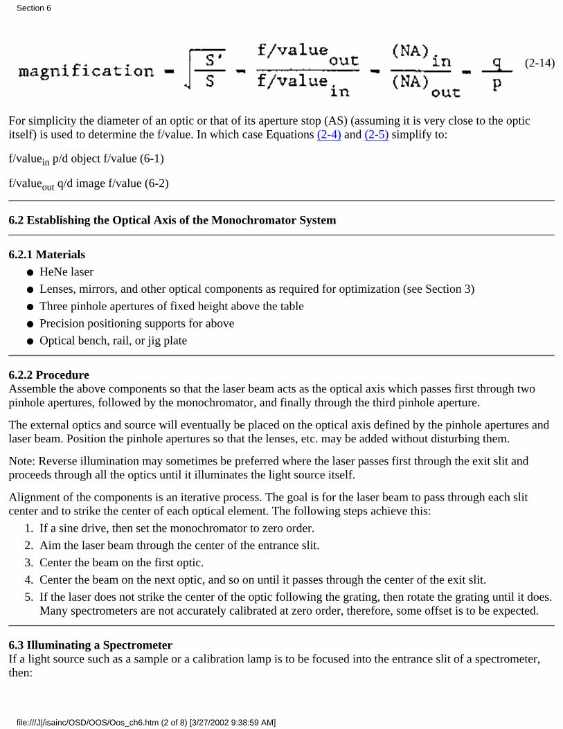
(214)

For simplicity the diameter of an optic or that of its aperture stop (AS) (assuming it is very close to the opticitself) is used to determine the f/value. In which case Equations (24) and (25) simplify to:

f/valuein p/d object f/value (61)

f/valueout q/d image f/value (62)

6.2 Establishing the Optical Axis of the Monochromator System

6.2.1 MaterialsHeNe laser●

Lenses, mirrors, and other optical components as required for optimization (see Section 3)●

Three pinhole apertures of fixed height above the table●

Precision positioning supports for above●

Optical bench, rail, or jig plate●

6.2.2 ProcedureAssemble the above components so that the laser beam acts as the optical axis which passes first through twopinhole apertures, followed by the monochromator, and finally through the third pinhole aperture.

The external optics and source will eventually be placed on the optical axis defined by the pinhole apertures andlaser beam. Position the pinhole apertures so that the lenses, etc. may be added without disturbing them.

Note: Reverse illumination may sometimes be preferred where the laser passes first through the exit slit andproceeds through all the optics until it illuminates the light source itself.

Alignment of the components is an iterative process. The goal is for the laser beam to pass through each slitcenter and to strike the center of each optical element. The following steps achieve this:

If a sine drive, then set the monochromator to zero order.1.

Aim the laser beam through the center of the entrance slit.2.

Center the beam on the first optic.3.

Center the beam on the next optic, and so on until it passes through the center of the exit slit.4.

If the laser does not strike the center of the optic following the grating, then rotate the grating until it does.Many spectrometers are not accurately calibrated at zero order, therefore, some offset is to be expected.

5.

6.3 Illuminating a SpectrometerIf a light source such as a sample or a calibration lamp is to be focused into the entrance slit of a spectrometer,then:

Section 6


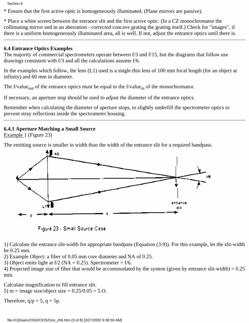
* Ensure that the first active optic is homogeneously illuminated. (Plane mirrors are passive).

* Place a white screen between the entrance slit and the first active optic. (In a CZ monochromator thecollimating mirror and in an aberration corrected concave grating the grating itself.) Check for "images", ifthere is a uniform homogeneously illuminated area, all is well. If not, adjust the entrance optics until there is.

6.4 Entrance Optics ExamplesThe majority of commercial spectrometers operate between f/3 and f/15, but the diagrams that follow usedrawings consistent with f/3 and all the calculations assume f/6.

In the examples which follow, the lens (L1) used is a single thin lens of 100 mm focal length (for an object atinfinity) and 60 mm in diameter.

The f/valueout of the entrance optics must be equal to the f/valuein of the monochromator.

If necessary, an aperture stop should be used to adjust the diameter of the entrance optics.

Remember when calculating the diameter of aperture stops, to slightly underfill the spectrometer optics toprevent stray reflections inside the spectrometer housing.

6.4.1 Aperture Matching a Small SourceExample 1 (Figure 23)

The emitting source is smaller in width than the width of the entrance slit for a required bandpass.

1) Calculate the entrance slitwidth for appropriate bandpass (Equation (39)). For this example, let the slitwidthbe 0.25 mm.2) Example Object: a fiber of 0.05 mm core diameter and NA of 0.25.3) Object emits light at f/2 (NA = 0.25). Spectrometer = f/6.4) Projected image size of fiber that would be accommodated by the system (given by entrance slitwidth) = 0.25mm.

Calculate magnification to fill entrance slit.5) m = image size/object size = 0.25/0.05 = 5.O.

Therefore, q/p = 5, q = 5p.

Section 6


6) Substituting into the lens Equation (316) gives p = 120 mm, and q = 600 mm.7) To calculate d, light must be collected at f/2 and be projected at f/6 to perfectly fill the grating.

Therefore, p/d = 2, d = 120/2 = 60 mm.

Therefore, aperture stop = full diameter of L1.

Projection f/value = 600/60 = 10.

In other words, the grating of the monochromator, even though receiving light collected at f/2, is underfilled bythe projected cone at f/10. All the light that could have been collected has been collected and no furtherimprovement is possible.

Example 2

If, however, the fiber emitted light at f/l, light collection could be further improved by using a lens in the sameconfiguration, but 120 mm in diameter. This would, however, produce an output f/value of

600/120 = f/5

Because this exceeds the f/6 of the spectrometer, maximum system light collection would be produced by a lenswith diameter

d = q/(f/value) = 600/6 = 100 mm

thereby matching the light collection etendue to the limiting etendue of the spectrometer.

The collection f/value is, therefore,

f/valuein = p/q = 120/100 = 1.2

Since etendue is proportional to the square of the (f/value)-l, about 70% of the available emitted light would becollected at f/1.2. See Section 3.

If the user had simply placed the fiber at the entrance slit with no entrance optics, only 3': of the available lightwould have been collected. (Light in this case was collected at the spectrometer's f/6 rather than the f/1.2 withetendue matching entrance optics).

6.4.2 Aperture Matching an Extended Source

Section 6


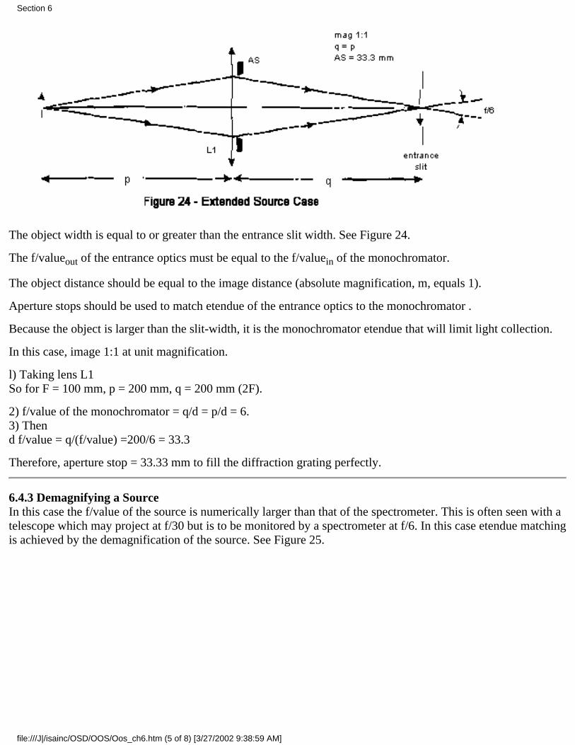
The object width is equal to or greater than the entrance slit width. See Figure 24.

The f/valueout of the entrance optics must be equal to the f/valuein of the monochromator.

The object distance should be equal to the image distance (absolute magnification, m, equals 1).

Aperture stops should be used to match etendue of the entrance optics to the monochromator .

Because the object is larger than the slitwidth, it is the monochromator etendue that will limit light collection.

In this case, image 1:1 at unit magnification.

l) Taking lens L1So for F = 100 mm, p = 200 mm, q = 200 mm (2F).

2) f/value of the monochromator = q/d = p/d = 6.3) Thend f/value = q/(f/value) =200/6 = 33.3

Therefore, aperture stop = 33.33 mm to fill the diffraction grating perfectly.

6.4.3 Demagnifying a SourceIn this case the f/value of the source is numerically larger than that of the spectrometer. This is often seen with atelescope which may project at f/30 but is to be monitored by a spectrometer at f/6. In this case etendue matchingis achieved by the demagnification of the source. See Figure 25.

Section 6


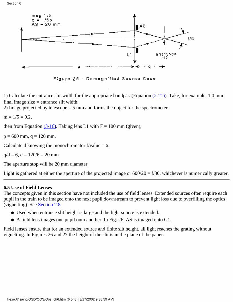
1) Calculate the entrance slitwidth for the appropriate bandpass(Equation (221)). Take, for example, 1.0 mm =final image size = entrance slit width.2) Image projected by telescope = 5 mm and forms the object for the spectrometer.

m = 1/5 = 0.2,

then from Equation (316). Taking lens L1 with F = 100 mm (given),

p = 600 mm, q = 120 mm.

Calculate d knowing the monochromator f/value = 6.

q/d = 6, d = 120/6 = 20 mm.

The aperture stop will be 20 mm diameter.

Light is gathered at either the aperture of the projected image or 600/20 = f/30, whichever is numerically greater.

6.5 Use of Field LensesThe concepts given in this section have not included the use of field lenses. Extended sources often require eachpupil in the train to be imaged onto the next pupil downstream to prevent light loss due to overfilling the optics(vignetting). See Section 2.8.

Used when entrance slit height is large and the light source is extended.●

A field lens images one pupil onto another. In Fig. 26, AS is imaged onto G1.●

Field lenses ensure that for an extended source and finite slit height, all light reaches the grating withoutvignetting. In Figures 26 and 27 the height of the slit is in the plane of the paper.

Section 6


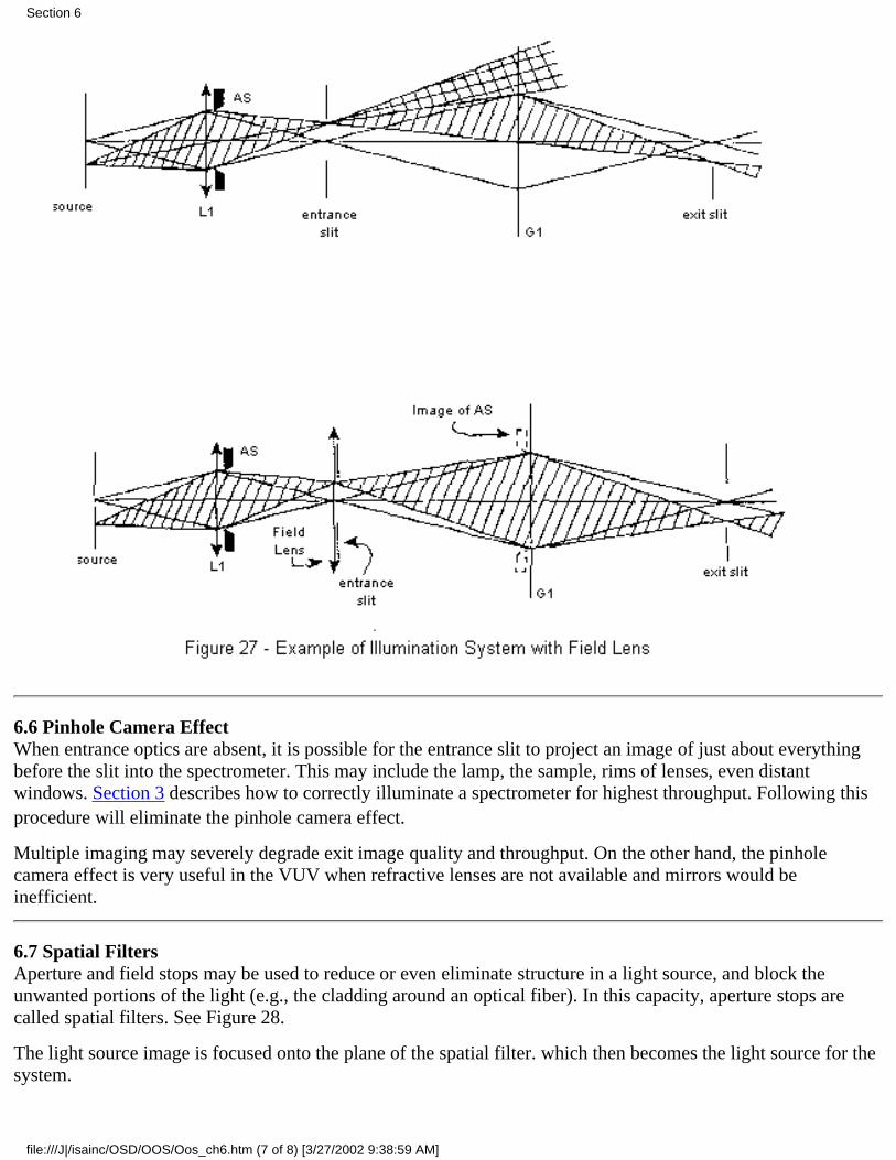
6.6 Pinhole Camera EffectWhen entrance optics are absent, it is possible for the entrance slit to project an image of just about everythingbefore the slit into the spectrometer. This may include the lamp, the sample, rims of lenses, even distantwindows. Section 3 describes how to correctly illuminate a spectrometer for highest throughput. Following thisprocedure will eliminate the pinhole camera effect.

Multiple imaging may severely degrade exit image quality and throughput. On the other hand, the pinholecamera effect is very useful in the VUV when refractive lenses are not available and mirrors would beinefficient.

6.7 Spatial FiltersAperture and field stops may be used to reduce or even eliminate structure in a light source, and block theunwanted portions of the light (e.g., the cladding around an optical fiber). In this capacity, aperture stops arecalled spatial filters. See Figure 28.

The light source image is focused onto the plane of the spatial filter. which then becomes the light source for thesystem.

Section 6


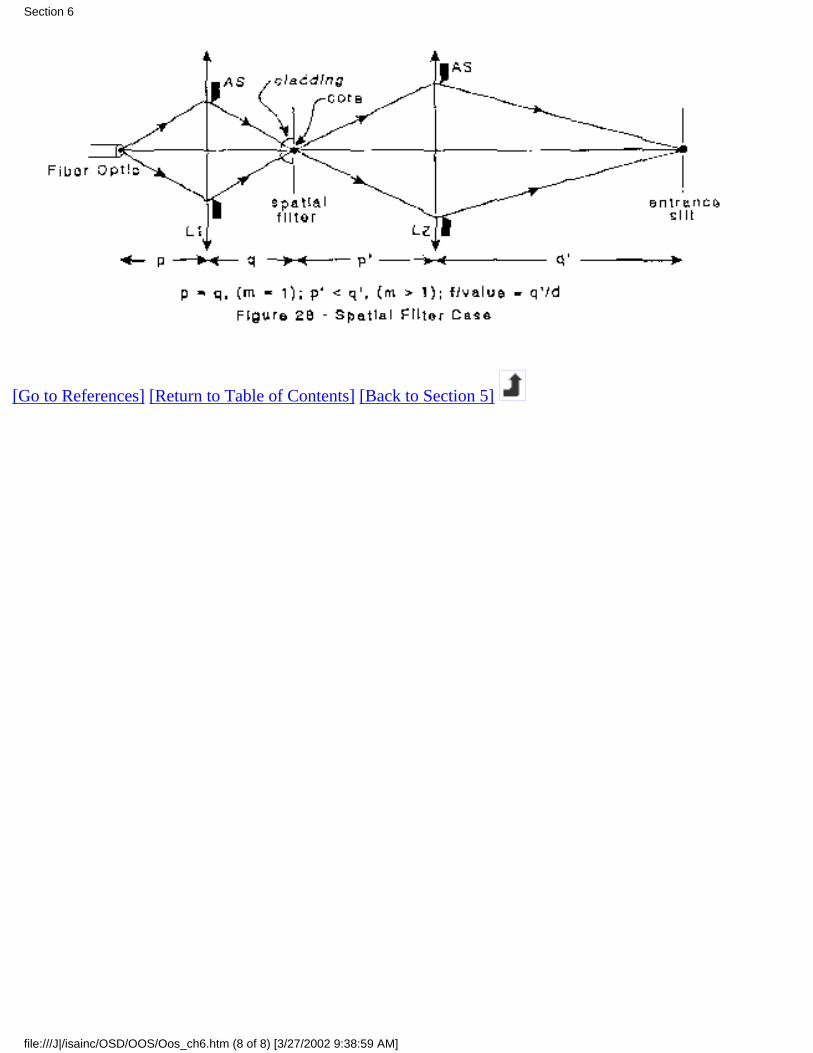
[Go to References] [Return to Table of Contents] [Back to Section 5]

Section 6


ACKNOWLEDGMENTSWe wish to thank the many people who have contributed their ideas and help in the writing of thistutorial. Thanks to Jean Flamand, JeanPierre Laude, and Bruno Touzet of JobinYvon, and Kim

Marshall of Instruments SA, Inc. Special thanks to Ramon Barnes of the University of Massachusetts andRick Feinberg of Western Washington University for their poignant and constructive comments.

BIBLIOGRAPHYl) Diffraction Gratings Ruled and Holograchic Handbook, published by Instruments SA, Inc., 6 OlsenAvenue, Edison, New Jersey 08820 USA and JobinYvon Div. d' Instruments SA., 1618 Rue du Canal91160 Longjumeau, France.

2) Chi, Chang H., Ed., "Periodic Structures, Gratings, Moire Patterns and Diffraction Phenomena", SPIEProc. 240 (1980).

3) Goldstein, S. A. and Walters, J. P., "A Review of Considerations for High Fidelity Imaging ofLaboratory Spectroscopic Sources Parts 1 and 2", Spectrochimica ACTA, 31B, 201316, (1976).

4) Hecht, E. and A. Zajac, Ontics, Addison Uesley, Reading, Massachusetts, ITRA ( 19 7 9).

5) James, J. F. and R. S. Sternburg, The Design of Optical Spectrometers Chapman & Hall Ltd., London,England, (1969).

6) Lerner, Jeremy M., Ed., "International Conference on the Application, Theory and Fabrication ofPeriodic Structures, Diffraction Gratings and Moire Phenomena", SPIE Proc. 503 (1984).

7) Lerner, Jeremy M., Ed., "International Conference on the Application, Theory and Fabrication ofPeriodic Structures, Diffraction Gratings and Moire Phenomena", SPIE Proc. 815 (1987).

8) Reader, J., "Optimizing CzernyTurner Spectrographs: A Comparison Between Analytic Theory andRay Tracing", J. Opt. Soc. Am. 59, (9), 11891196. (1969).

9) Reader, J., "What is Dynamic Dispersion", Applied Optics 20, (13), 21732172, (1981).

10) Shafer, A. B., Megill, L. R., and Droppleman, L., "Optimization of the CzernyTurner", J. Opt. Soc.Am. 54, (7), 879887 (1964).

11) Stroke, G. W., Handbuch der Physik XXIX, Springer Berlin, (1967), (Chapter is in English and iscomprehensive).

12) Thevenon, A., Flamand, J., Laude, J. P., Touzet, B., and Lerner, J. M., "Aberration Corrected PlaneGratings", SPIE Proc 815, 136145, (1987).

° Instruments SA, Inc. 1988

[Return to Table of Contents] [Back to Section 6]

References

file:///J|/isainc/OSD/OOS/REF.HTM [3/27/2002 9:39:10 AM]

Documents

The Optics Of Spectroscopy...2.3 Czerny Turner Configuration 2.4 Czerny Turner/Fastie Ebert PGS Aberrations 2.4.1 Aberration Correcting Plane Gratings 2.5 Concave Aberration Corrected