Embed Size (px)
Citation preview
THE OPTIMAL ASSIGNMENT PROBLEM
A Thesis
Presented to
the Division of Mathematics
Emporia State University
In partial Fulfillment
of the Requirements for the Degree
Master of Science
by
Laura J. Oliver ::
July, 1992

\' i
AN ABSTRACT OF THE THESIS
Laura J. Oliver for the Master of Science
in Mathematics presented on May 7 .1992
Abstract Approved: ~ J1.~
This thesis is intended for an audience familar with basic linear algebra.
The topic covered is the assignment problem. Chapter I is the introduction to the
problem and the assumptions made. Chapter 2 discusses Kuhn's algorithm for solving
the assignment problem. An example is done throughout the discussion. Chapter 3
discusses the Hungarian method for solving the assignment problem. An example fol
lows this method. Chapter 4 discusses finding the optimal solution and Chapter 5
summarizes the two methods and gives a direction for further study.

~a
UOISIAIQ Jor~W ;:lql 10J P;:lA01ddy
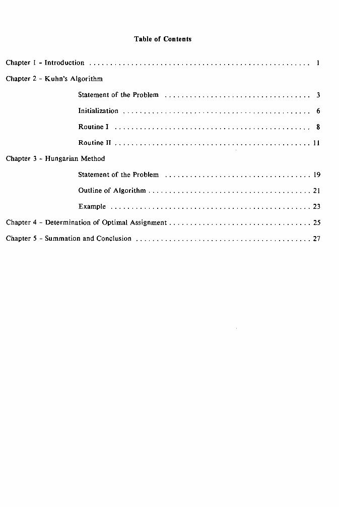
Table of Contents
Chapter I - Introduction .
Chapter 2 - Kuhn's Algorithm
Statement of the Problem 3
Chapter 3 - Hungarian Method
Initialization 6
Routine I 8
Routine II II
Statement of the Problem 19
Outline of Algorithm 21
Example 23
Chapter 4 - Determination of Optimal Assignment 25
Chapter 5 - Summation and Conclusion 27
CHAPTER I
Introduction
The assignment problem is a well studied problem in combinatorics and operations
research. The problem has arisen in a variety of contexts and, hence, it has received many
names such as the marriage problem, the maximal transversal problem, and the name
which we will use in this paper, the assignment problem.
Let us first describe it in the context of the marriage problem. Given n men, mI,
m2, ms' ... , mn and k women, wI' w2 ' ws' ... , Wk we assign to each pair of a woman
and man a I if they are willing to marry and a 0 if not. The marriage problem asks, "What
is the maximum number of marriages possible." Actually the problem considered in this
work is a bit more general. Suppose to each man, and each woman, a positive integer
could be assigned (a happiness rating?) to their future as a married couple. The Question
addressed here is how the marriages should be arranged to maximize the total level of
happiness. [4, p.620]
The problem in this work will consider the case n=k. Mathematically stated the
assignment problem is as follows: Let R be an n x n matrix with positive integer entries.
The optimal assignment problem consists of choosing n entries, so that no two chosen
entries come from the same row or column and such that the sum of the entries is
maximized.
Consider the assignment problem in the following context. Given n individuals
and n jobs, the entry in the ith row jth column, rij , of R denotes the rating value given to
the i th individual doing the jth job. The optimal assignment problem seeks to determine
the "best" possible pairing of individuals to jobs.
MathematicallY, the assignment problem can be stated as follows:
" Maximize: L Tij with (h, b jg, ... , jn) I,j= 1 I
a permutation of (I, 2, 3, ... ,n)
The General Assignment Problem makes several assumptions:
A I. The number of individuals equals the number of jobs.
A2. Each individual can do each job.
A3. No two individuals are paired to the same job; and no individual is paired to more than one job.
This paper will cover two methods of solving the General Assignment Problem.
First, Kuhn's method will be discussed which deals with using the dual of the problem and
second, the Hungarian method which uses a more direct approach to solving the problem.
2

CHAPTER 2
Kuhn's Algorithm
STATEMENT OF THE PROBLEM
The first algorithm to be discussed, Kuhn's method, solves the problem by finding
a solution to what Kuhn referred to as a dual problem. Kuhn's dual is stated in the
following manner
minimize EII
(uj + VI) i=1
Subject to Uj + vj ~ rjj
Note that if uj's and vJ,'s can be found such that uj + vir = Til,' where vI, is the job
assigned to individual i and (h, j2' js' ... , jn) is a permutation of ( I, 2, 3, ... , n ), then
the original maximizing problem has been solved.
Since uj + v ~ rjj for all i, j J
II II
Then E (Uj + Vi ) ~ E TIJ, with (h, h, h, ..., jn ) a 1=1 i=1
permutation of (I, 2, 3, ... , n)
II II
Then min E (uj + Vi) ~ max ETu, rjj 1=1 i=1
Thus if there exists a combination of Uj' and vJ, such that uj + vI, = TIj,
for i = 1, 2, 3, ... n, and (jl' j2' js' ... , jn) is a permutation of (I, 2, 3, ... , n) then the
minimization problem and the original maximization problem have been solved.
It is interesting to note that this method predates the simplex method.[l,p.206] The
label of dual in Kuhn's method is consistent with the use of that term in the theory of
3
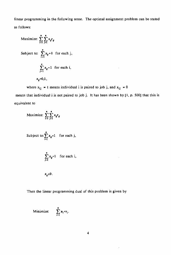
linear programming in the following sense. The optimal assignment problem can be stated
as follows:
II II
Maximize: L LXI'iJ ;=1 }=1
Subject to: LII
x4I =1 for each j, 1= I
LII
x4I = 1 for each i, 1=1
x4I "'O,I,
where xij = 1 means individual i is paired to job j, and xij = 0
means that individual i is not paired to job j. It has been shown by [1, p. 500] that this is
equivalent to
II II
Maximize: L L xI'41 1=1 1=1
II
Subject to:LxiJ=1 for each j, ;=1
II
Lx4I =1 for each i, 1=1
Xii~O.
Then the linear programming dual of this problem is given by
II
Minimize: L"I+v;, i=1
4

Subject to: uj + Vj ~ r jj .
Uj, vj unrestricted.
Kuhn's algorithm considers the problem from the dual point of view. Kuhn has
developed a computational method that will use this dual in an effective manner.
Recall the assumptions Al - A3 made in Chapter 1. For Kuhn's method we also
assume that the entries r jj in the R matrix are positive integers. Before discussing this
method further some definitions are required.
An assignment is a set of k pairings, k ~ n, of individuals to jobs. A transfer is a
shifting of individuals paired to jobs so as to increase the number of pairings. An
individual i is Qualified to do job j if Uj + vj = rij . Note each individual can do each job,
but each individual is not qualified to do each job.
The following notation will also be used. Let Q denote the qualified matrix, with
entries qij = 1 if individual i is qualified for job j; and 0 otherwise.
A L in (i,j) in Q implies that the ith individual has been assigned the jth job.
Kuhn's method of solving the assignment problem has three major components,
first, the initialization stage which initializes the variables and gives an initial assignment;
second, Routine I, which is used to attempt transfers to improve a given assignment; and
third, Routine II, used to decrease u's and v's to increase the number of individuals
qualified for jobs.
5

INITIALIZATION
In the initialization stage Kuhn used the following method for determining the
initial uj's and v/s.
Let aj be the maximum of {rjj I I ~ j ~ n } and let a = L• aj' Let bj be the i=1
• maximum of {rjj I I ~ i ~ n } and let b = L hi"
j=1
Since we want to minimize L• uj + 'Vj , we will use the minimum of a and b. i=1
If a ~ b let uj = aj i = I, 2, 3, ... ,n and
'Vj = 0 j = I, 2, 3, ... , n.
If a > b let uj = 0 i = I, 2, 3, ... , nand
v.1
= b·J j = I, 2, 3, ... , n.
Clearly either choice for the initial assignment of Uj'S and 'V/s is a feasible solution
to the dual problem and preference is given to the one producing the smaller initial sum.
Once the uj's and v/s have been initialized the Qualified matrix Q must be
constructed. Recall the entries, Qjj' of Q are I if Uj + 'Vj = rij and 0 otherwise. Once Q
has been constructed, an assignment must be made. Kuhn's method for creating an initial
assignment is as follows: Proceed down column j for j = I, 2, 3, ... , n. The first I
located in column j that does not have a 1* in its row becomes a 1*. Proceed to the next
column until all columns have been checked. After this is completed, there should be no
row or column with more than one 1* in it. The initial assignment is done; Q is ready to
be sent to Routine I. An example of the initialization of the u's and v's along with the
construction of Q follows.
6

9 9 8 9 7 1 S 3 6 6
Given the rating matrix R = 13 4 4 3 21 recall that ai is the maximum 4 4 4 S 3 3 3 2 8 7
II II
entry in row i, L ai = a, bj is the maximum entry in column j, and L bj = b. Since in our i=l i=1
example, a = 32 and b = 42, the following initial assignment is made. Let u l = 9, u2 = 6,
ua = 4, u4 = 5, u6 = 8; and vi = 0 for j = 1, 2, 3, ... n. Given these u's and v's, the
following Q is produced.
1 1 0 1 0 o o 0 1 1
Q= 10 1 1 o 0 o o 0 1 0 o o 0 1 0
Next an initial assignment is needed. Recall Kuhn's method for an initial
assignment is to proceed down each column. If a I is found without a 1* in its row, then
the I becomes a 1*, Using this method the initialization of Q produces the following.
1· 1 0 1 0 o 0 0 1· 1
Q = 10 1· 1 0 0 00010 00010
Now Q has been constructed and an initial assignment has been made. Q is ready
for Routine I.
7
ROUTINE I
Routine I is used to determine if it is possible to make a transfer in order to
increase the number of pairings in the given assignment. Given the Q matrix, Routine I
has two possible outcomes:
IA - A transfer has been made, thus improving the number of pairings in the assignment. The altered Q is sent to Routine I to determine if any other transfers are possible.
IB - No transfers were made in the Q entered in Routine I. Q is now ready to be sent to Routine II.
An equivalent definition for a transfer is needed before Routine I can be
discussed. A transfer is a shifting of l's (people qualified for jobs) and l*'s (people
assigned to jobs) to increase the number of l*'s.
A definition for an essential row is also needed before discussing the algorithm for
Routine I. A row that has a 1* that is needed for a transfer, but can not be used, is an
essential row. This row is termed essential because the individual assigned to this job can
not be transferred to a different job.
Once entering Routine I, a check is made to determine if each column has a 1*. If
a column is found that does not have a 1* in it, then a search for a 1 in that column is
made, so a transfer can be attempted. If a 1 is not found a transfer can not be attempted
and that column is passed over.
Recall that no column or row can have more than one 1*. So if a 1 is found in the
column, say in row k, before it can be shifted to a 1* a check of row k is done to
determine if there is already a 1* in the kth row. If not, the shift of that 1 to a 1* is done.
A transfer has been completed and outcome IA has occurred. Now that Q has been
altered, Routine I must be performed again to check for any other transfers.
8
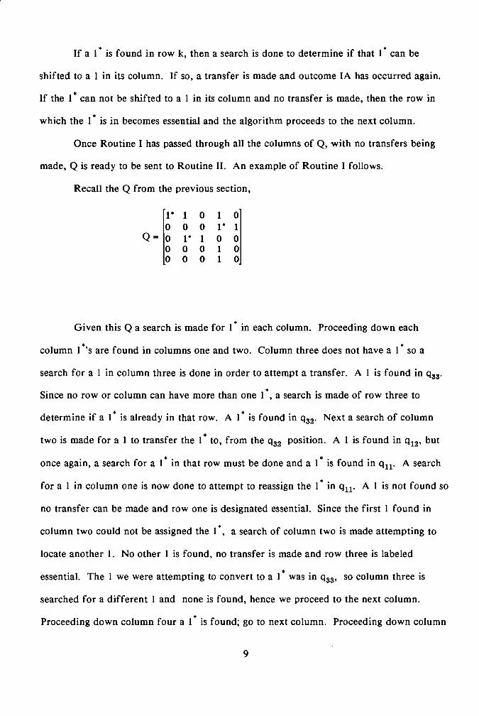
If a 1* is found in row k, then a search is done to determine if that 1* can be
shifted to a 1 in its column. If so, a transfer is made and outcome IA has occurred again.
If the 1* can not be shifted to a 1 in its column and no transfer is made, then the row in
which the 1* is in becomes essential and the algorithm proceeds to the next column.
Once Routine I has passed through all the columns of Q, with no transfers being
made, Q is ready to be sent to Routine II. An example of Routine I follows.
Recall the Q from the previous section,
. 1* 1 0 1 0 0 0 0 1· 1
Q= 10 1· 1 0 0 0 0 0 1 0 0 0 0 1 0
Given this Q a search is made for 1* in each column. Proceeding down each
column l*'s are found in columns one and two. Column three does not have a 1* so a
search for a 1 in column three is done in order to attempt a transfer. A 1 is found in qss'
Since no row or column can have more than one 1*, a search is made of row three to
determine if a 1* is already in that row. A 1* is found in qS2. Next a search of column
two is made for a 1 to transfer the 1* to, from the qS2 position. A 1 is found in Q12' but
once again, a search for a 1* in that row must be done and a 1* is found in qu. A search
for a 1 in column one is now done to attempt to reassign the 1* in qu. A 1 is not found so
no transfer can be made and row one is designated essential. Since the first 1 found in
column two could not be assigned the 1*, a search of column two is made attempting to
locate another 1. No other 1 is found, no transfer is made and row three is labeled
essential. The 1 we were attempting to convert to a 1* was in q33' so column three is
searched for a different 1 and none is found, hence we proceed to the next column.
Proceeding down column four a 1* is found; go to next column. Proceeding down column
9

five, no 1* is found, the search for a I is done. A I is found in Q2S' Row two must then
be searched for a 1* and a 1* is found in Q24' Then a I in column four is needed to
attempt to transfer the 1* from Q24' A I is found in q14' but the same result that occurred
when the first transfer was attempted will also occur here. That is, the 1* in qll can not
be reassigned so no transfer is done. If row one had not already been labeled essential it
would now be labeled as such.
Column four is now searched for another I to attempt to reassign the 1* that is in
q24' A I is found in q44' A search is made of row four for a 1*. Since one is not found,
the I in q44 is assigned the 1*. The 1* in q24 becomes a I and the I in Q2s becomes a 1*.
The transfer has now been completed. Once this has been done all previously essential
rows become inessential and the altered Q is sent to Routine I again. The altered Q is as
follows.
r 1* 1 0 1 0 0
Q = I0 0 l'
0 1
1 0
I' 0
0 0 0 l' 0 0 0 0 1 0
When entering Routine I a transfer will again be attempted using the I in Qss'
When the transfer still can not be completed, rows one and three will once again be
designated as essential. All the other columns of Q have I*'s in them so no other transfers
are attempted. Since no transfers were made Q is now ready for Routine II.
10

ROUTINE II
Upon entering Routine II all possible transfers have been made. The following
definitions will be useful in discussing Routine II.
An essential column is a column with a 1* in an inessential row. Since all essential
rows also have 1* in them the number of essential rows and columns equals the number of
* . Q1 's In .
In this method of solving the General Assignment Proble~, the only acceptable
pairings of individuals to jobs are those of individuals Qualified to jobs, that is uj + vi = rjj'
An optimal solution is an assignment of n pairings (n l*'s in Q). Note an assignment is a
set of k pairings such that k ~ n, assumptions Al - A3 hold, and all rij are positive
integers. Recall that in solving the dual we want to minimize EII
Uj + vi which we will i=1
refer to as the budget.
Routine II is used to determine whether an optimal solution has been found. If an
optimal solution has not been found, a reduction in the budget will be made.
Before the algorithm for Routine II can be discussed, the relationship between the
number of essential rows, ER, inessential rows, IER, essential columns, EC, and inessential
columns, IEC, must be understood. Note that EC + IEC = nand -ER + IER = n. As stated
before ER + EC = the number of 1* in Q. Hence, ER + EC ~ n. The only time ER + EC
= n is when ER = 0 and EC = n. The reason for this is that if ER + EC = n, then there are
n l*'s in Q. This would mean that every column had a 1* in it, so it is impossible that a
transfer is attempted, but not completed. Therefore ER would be zero.
The next relationship that is needed is between ER and IEC. By the trichotomy
principle there are three cases.
11

CASE I IEC < ER, adding EC to both sides of this equation leads to the following:
IEC + EC < ER + EC. Since IEC + EC = n and ER + EC ~ n, we have this equation: n < ER + EC ~n.
This is a contradiction.
CASE II IEC = ER, adding EC to both sides of this equation then leads to IEC + EC = ER + EC. Which leads to n = ER + EC ~ n. This implies that ER + EC = n, therefore ER = 0 and EC = n. This is the trivial case.
CASE III IEC> ER, which follows directly.
The last relationship that needs to be understood is between EC and IER. Since
IEC = n - EC and ER = n - IER, then the above yields the following relationship between
EC and IER. Either EC = IER which implies ER = 0, EC = n or EC < IER. With these
relationships clarified, the algorithm for Routine II is discussed.
Upon entering Routine II the essential rows have been recorded, and next the
essential columns must be recorded. Once this is done, if there are no inessential columns,
then there are n essential columns and the assignment of I· is an optimal solution. Thus
the General Assignment Problem and its dual have been solved.
If there are inessential columns, then a reduction in the budget can be made. To
determine the amount of the reduction, first compute d, the minimum of u j + Vi - r jj
taken over all inessential i's and j's. Once d has been computed there are two mutually
exclusive cases.
CASE I Uj > 0 for all inessential rows. If this occurs, compute m, the minimum of d and Uj taken over all inessential i. Then the reduction in the budget is done as follows:
Replace Uj by Uj - m for all inessential i. Replace Vi by Vi + m for all essential j.
Recall that EC < IER so this will always produce a budget reduction.
12
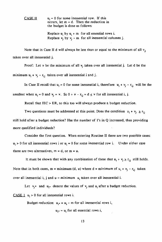
CASE II u j = 0 for some inessential row. If this occurs, let m = d. Then the reduction in the budget is done as follows:
Replace uj by uj + m for all essential rows i. Replace vj by vj - m for all inessential columns j.
Note that in Case II d will always be less than or equal to the minimum of all Vj
taken over all inessential j.
Proof: Let v be the minimum of all vi taken over all inessential j. Let d be the
minimum Uj + vi - rjj taken over all inessential i and j.
In Case II recall that Uj = 0 for some inessential i, therefore Uj + vi - rjj will be the
smallest when Uj = 0 and vi = v. So 0 + v - rjj = d ~ v for all inessential i, j.
Recall that IEC > ER, so this too will always produce a budget reduction.
Two questions must be addressed at this point. Does the condition uj + vi ~ rjj
still hold after a budget reduction? Has the number of l's in Q increased, thus providing
more qualified individuals?
Consider the first question. When entering Routine II there are two possible cases:
Uj > 0 for all inessential rows i or Uj = 0 for some inessential row i. Under either case
there are two alternatives, m = d, or m = u.
It must be shown that with any combination of these that Uj + vj ~ rjj still holds.
Note that in both cases, m = minimum (d, u) where d = minimum of Uj + vi - rij taken
over all inessential i, j and U = minimum Uj taken over all inessential i.
Let vi * and Uj* denote the values of vi and Uj after a budget reduction.
CASE 1 Uj > 0 for all inessential rows i.
Budget reduction: Uj* = Uj - m for all inessential rows i,
Uj* = Uj for all essential rows i,
13
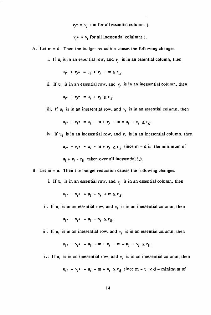
* = v + m for all essential columns j,Vi J
vi * = vJ for all inessential colulmns j.
A. Let m = d. Then the budget reduction causes the following changes.
1. If uj is in an essential row, and vi is in an essential column, then
uj* + vJ* = Uj + vJ + m ~ rij'
11. If uj is in an essential row, and vJ is in an inessential column, then
Uj* + vi * = Uj + vi ~ rjj'
iii. If uj is in an inessential row, and vJ is in an essential column, then
Uj* + vJ* = Uj - m + vJ + m = Uj + vi ~ rij'
iv. If uj is in an inessential row, and vJ is in an inessential column, then
Uj* + vi * = Uj - m + vJ ~ rij since m = d is the minimum of
Uj + vi - r jj taken over all inessential i,j.
B. Let m = u. Then the budget reduction causes the following changes.
1. If Uj is in an essential row, and vJ is in an essential column, then
Uj* + vi * = uj + vJ + m ~ r jj .
11. If Uj is in an essential row, and vi is in an inessential column, then
U j * + vi * = uj + vJ ~ rij'
111. If Uj is in an inessential row, and vJ is in an essential column, then
Uj* + vi * = uj + m + vi - m = uj + vJ ~ rij'
IV. If Uj is in an inessential row, and vJ is in an inessential column, then
Uj* + vi * = uj - m + vi ~ r jj since m = U ~ d = minimum of
14

uj + VJ - r jj over all inessential i,j.
Therefore if u j > 0 for all inessential i, then after the budget reduction is made,
the condition that Uj + vJ ~ rjj still holds.
CASE 2 uj = 0 for some inessential row i.
Budget reduction: uj* = uj + m for all essential rows i,
uj* = uj for all inessential rows i,
vJ• = vi - m for all inessential columns j,
vi. = vJ for all essential columns j.
Recall that in Case II, uj = 0 for some inessential row i, that m = d.
Then the budget reduction causes the following changes
i. If uj is in an essential row, and vi is in an essential column, then
Uj* + vi. = uj + m + vJ ~ rij'
11. If uj is in an essential row, and vi is in an inessential column, then
Uj* + vi. = Uj + m + vJ - m = Uj + vi ~rjj'
111. If uj is in an inessential row, and vJ is in an essential column, then
Uj* + vi. = Uj + vi ~ rjj'
IV. If uj is in an inessential row, and vJ is in an inessential column, then
Uj* + vi. = Uj + vi - m ~ rij since m = d is minimum of
Uj + vi - r jj taken over inessential i,j.
Next, consider the second question: Will the number of l's in Q increase after a
budget reduction?
Since d is the minimum of Uj + vi -rjj' if m = d then at least one new I will
15
definitely be introduced. If m = u then a new 1 may not be introduced after the first
budget reduction. But when Routine II is applied again, then u j = 0 for some inessential i,
so Case II will occur, m will equal d, thus a new 1 will be introduced. So even if we go
through Routine II and a new 1 is not introduced, then when we go through it the next
time a new 1 will definitely be introduced.
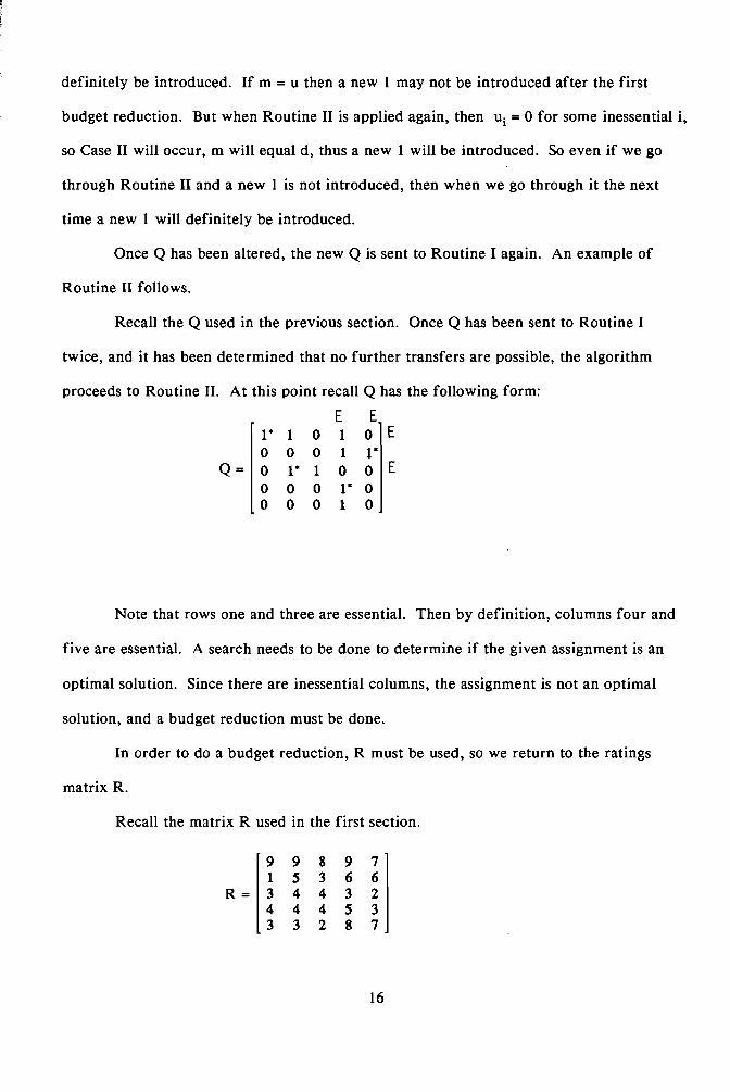
Once Q has been altered, the new Q is sent to Routine I again. An example of
Routine II follows.
Recall the Q used in the previous section. Once Q has been sent to Routine I
twice, and it has been determined that no further transfers are possible, the algorithm
proceeds to Routine II. At this point recall Q has the following form:
E E I- I 0 1 OlE 0 0 0 1 1
Q = 1 0 I- I 0 OlE 0 0 0 1- 0 0 0 0 1 0
Note that rows one and three are essential. Then by definition, columns four and
five are essential. A search needs to be done to determine if the given assignment is an
optimal solution. Since there are inessential columns, the assignment is not an optimal
solution, and a budget reduction must be done.
In order to do a budget reduction, R must be used, so we return to the ratings
matrix R.
Recall the matrix R used in the first section.
9 9 897 1 S 3 6 6
R=13 4 4 3 2 4 4 4 S 3 33287
16
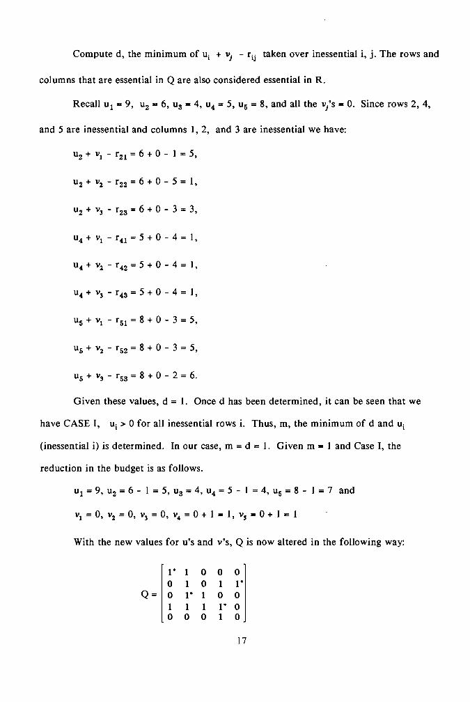
Compute d, the minimum of uj + vJ - r jj taken over inessential i, j. The rows and
columns that are essential in Q are also considered essential in R.
Recall u 1 = 9, u2 = 6, u3 = 4, u4 = 5, u5 = 8, and all the v/s = O. Since rows 2, 4,
and 5 are inessential and columns 1, 2, and 3 are inessential we have:
u2 + VI - = 6 + 0 - 1 = 5,r21
u 2 + v2 - r 22 = 6 + 0 - 5 = 1,
- =6 + 0 - 3 = 3,u2 + v3 r23
u4 + VI - = 5 + 0 - 4 = 1,r41
u 4 + v2 - r 42 = 5 + 0 - 4 = 1,
u 4 + v3 - r 43 = 5 + 0 - 4 = 1,
u5 + VI - = 8 + 0 - 3 = 5,r 51
u 5 + v2 - = 8 + 0 - 3 = 5,r52
u 5 + v3 - r53 = 8 + 0 - 2 = 6.
Given these values, d = 1. Once d has been determined, it can be seen that we
have CASE I, Uj > 0 for all inessential rows i. Thus, m, the minimum of d and Uj
(inessential i) is determined. In our case, m = d = 1. Given m = 1 and Case I, the
reduction in the budget is as follows.
u1 = 9, u2 = 6 - 1 = 5, u3 = 4, u4 = 5 - 1 = 4, u5 = 8 - 1 = 7 and
VI = 0, v2 = 0, v3 = 0, v4 = 0 + 1 = 1, Vs = 0 + 1 = 1
With the new values for u's and v's, Q is now altered in the following way:
l' 1 0 0 0 0 1 0 1 l'
Q= 1 0 I" 1 0 0 1 1 1 I" 0 0 0 0 1 0 .
17
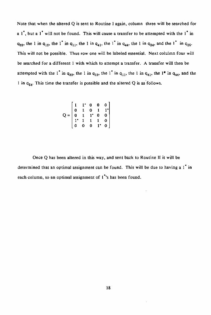
Note that when the altered Q is sent to Routine I again, column three will be searched for
a 1*, but a 1* will not be found. This will cause a transfer to be attempted with the 1* in
Q32' the 1 in Q12' the 1* in Qll' the 1 in Q41' the 1* in Q44' the 1 in Q24' and the 1* in Q26.
This will not be possible. Thus row one will be labeled essential. Next colulmn four will
be searched for a different 1 with which to attempt a transfer. A transfer will then be
attempted with the 1* in Q32' the 1 in Q12' the 1* in Qll' the 1 in Q41' the 1* in Q44' and the
1 in Q64. This time the transfer is possible and the altered Q is as follows.
1 I" 0 0 0 0 1 0 1 I"
Q= 10 1 I" 0 0 I" 1 1 1 0 0 0 0 I" 0
Once Q has been altered in this way, and sent back to Routine II it will be
determined that an optimal assignment can be found. This will be due to having a 1* in
each column, so an optimal assignment of 1*'s has been found.
18

CHAPTER 3
Hungarian Method
STATEMENT OF THE PROBLEM
The second method of solving the General Assignment Problem is the Hungarian
Method. Recall assumptions Al - A3 made in Chapter I. For the Hungarian Method, we
also assume that the problem is a minimization problem, but given a maximization problem
it can easily be converted to a minimization problem by multiplying all entries in the
rating matrix R by -1. Before continuing with the discussion of the Hungarian Method,
some notation and definitions are needed.
Since the Hungarian method is one of minimization, the matrix which is used to
determine an optimal assignment is referred to as ~, the cost matrix. The entry Cij in C
represents the cost of individual i doing job j.
As before, an assignment is a set of n entries with no two entries from the same
row or column. The sum of the entries of an assignment is referred to as the cost of the
assignment.
The last definition needed is that of an optimal assignment. which is the
assignment with the smallest possible cost.
The basis for the Hungarian method is the following theorem.
Theorem - If a number is added to or subtracted from all of the entries of anyone
row or column of a cost matrix, then an optimal assignment for the resulting cost matrix is
also an optimal assignment for the original cost matrix.
Proof:
Let LII
eiJ where <h, j2' j3' ... jn) is a permutation of (1, 2, 3, ... n) i, j=l I
be the optimal assignment.
19
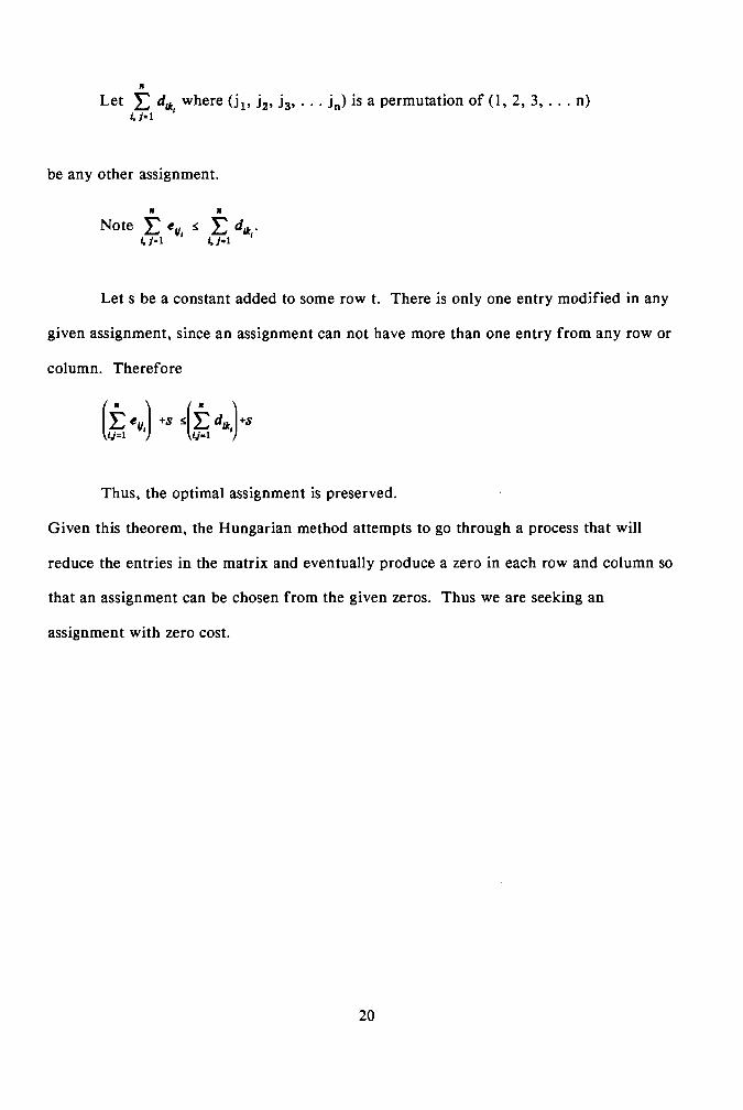
" Let L djk where (j l' j2' j3' ... jn) is a permutation of (l, 2, 3, ... n) i, j.1 I
be any other assignment.
" " Note L ell :s: L dlk ·
I, j.1 I I, j.1 I
Let s be a constant added to some row t. There is only one entry modified in any
given assignment, since an assignment can not have more than one entry from any row or
column. Therefore
(It ell,) +8 :s:(~ dlk,) +8
Thus, the optimal assignment is preserved.
Given this theorem, the Hungarian method attempts to go through a process that will
reduce the entries in the matrix and eventually produce a zero in each row and column so
that an assignment can be chosen from the given zeros. Thus we are seeking an
assignment with zero cost.
20
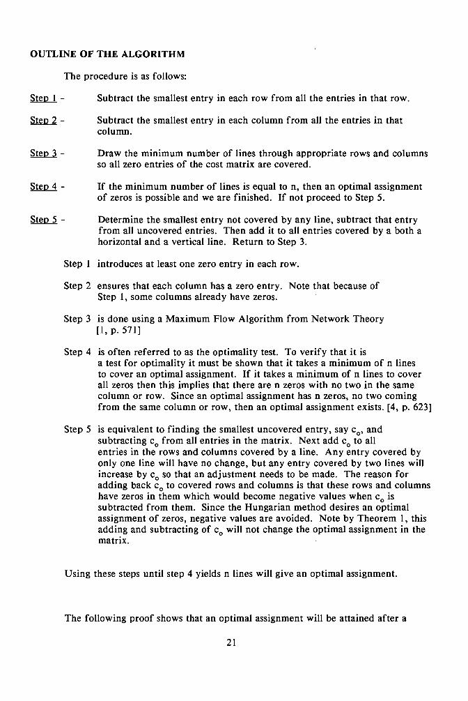
OUTLINE OF THE ALGORITHM
The procedure is as follows:
~- Subtract the smallest entry in each row from all the entries in that row.
Step 2 - Subtract the smallest entry in each column from all the entries in that column.
~- Draw the minimum number of lines through appropriate rows and columns so all zero entries of the cost matrix are covered.
Step 4 - If the minimum number of lines is equal to n, then an optimal assignment of zeros is possible and we are finished. If not proceed to Step 5.
Step 5 - Determine the smallest entry not covered by any line, subtract that entry from all uncovered entries. Then add it to all entries covered by a both a horizontal and a vertical line. Return to Step 3.
Step I introduces at least one zero entry in each row.
Step 2 ensures that each column has a zero entry. Note that because of Step I, some columns already have zeros.
Step 3 is done using a Maximum Flow Algorithm from Network Theory [I, p. 571]
Step 4 is often referred to as the optimality test. To verify that it is a test for optimality it must be shown that it takes a minimum of n lines to cover an optimal assignment. If it takes a minimum of n lines to cover all zeros then this implies that there are n zeros with no two in the same column or row. Since an optimal assignment has n zeros, no two coming from the same column or row, then an optimal assignment exists. [4, p. 623]
Step 5 is equivalent to finding the smallest uncovered entry, say co' and subtracting Co from all entries in the matrix. Next add Co to all entries in the rows and columns covered by a line. Any entry covered by only one line will have no change, but any entry covered by two lines will increase by Co so that an adjustment needs to be made. The reason for adding back Co to covered rows and columns is that these rows and columns have zeros in them which would become negative values when Co is subtracted from them. Since the Hungarian method desires an optimal assignment of zeros, negative values are avoided. Note by Theorem I, this adding and subtracting of Co will not change the optimal assignment in the matrix.
Using these steps until step 4 yields n lines will give an optimal assignment.
The following proof shows that an optimal assignment will be attained after a
21

OUTLINE OF THE ALGORITHM
The procedure is as follows:
~- Subtract the smallest entry in each row from all the entries in that row.
Step 2 - Subtract the smallest entry in each column from all the entries in that column.
Step 3 - Draw the minimum number of lines through appropriate rows and columns so all zero entries of the cost matrix are covered.
Step 4 - If the minimum number of lines is equal to n, then an optimal assignment of zeros is possible and we are finished. If not proceed to Step 5.
Step 5 - Determine the smallest entry not covered by any line, subtract that entry from all uncovered entries. Then add it to all entries covered by a both a horizontal and a vertical line. Return to Step 3.
Step 1 introduces at least one zero entry in each row.
Step 2 ensures that each column has a zero entry. Note that because of Step 1, some columns already have zeros.
Step 3 is done using a Maximum Flow Algorithm from Network Theory [l,p.571]
Step 4 is often referred to as the optimality test. To verify that it is a test for optimality it must be shown that it takes a minimum of n lines to cover an optimal assignment. If it takes a minimum of n lines to cover all zeros then this implies that there are n zeros with no two in the same column or row. Since an optimal assignment has n zeros, no two coming from the same column or row, then an optimal assignment exists. [4, p. 623]
Step 5 is equivalent to finding the smallest uncovered entry, say co' and subtracting Co from all entries in the matrix. Next add Co to all entries in the rows and columns covered by a line. Any entry covered by only one line will have no change, but any entry covered by two lines will increase by Co so that an adjustment needs to be made. The reason for adding back Co to covered rows and columns is that these rows and columns have zeros in them which would become negative values when Co is subtracted from them. Since the Hungarian method desires an optimal assignment of zeros, negative values are avoided. Note by Theorem 1, this adding and subtracting of Co will not change the optimal assignment in the matrix.
Using these steps until step 4 yields n lines will give an optimal assignment.
The following proof shows that an optimal assignment will be attained after a
21

- -
- -
finite number of iterations of Step I through Step 5.
To show finiteness we need to show that the reduced costs are always positive.
Let Sr = {iI' i2, ••• ip } a set of uncovered rows in C.
Let Sr = set of covered rows in C. Note that Sr has n-p elements.
Let Sc = {jl' j2' ... jq } set of uncovered columns in C.
Let Sc = set of covered columns in C. Note that Sc has n - q elements.
So p = number of elements in Sr and q = number of elements in Sc.
Let eiJ = the entries in C after Steps I and 2.
Let eiJ = the entries in C after a reduction from Step 5 has been made.
Let n = number of rows or columns in C.
Let Co = smallest uncovered entry found in Step 5.
Let k = maximum number of zeros in an assignment = minimum number of lines needed to cover all zeros in C. [4, 623]
"" ." Proof: E E e,j - E E c,J = reduced cost
1=1 j=1 1=1 j=1
". .. E E elj - E E c,J=
1=1 j=1 1=1 j=1
E CD + E 0 + E 0 + E -CD S S - - - ,x • S,xS. S,xS. S,xS.
= pqc - (n - p)(n - q)c = n(p + q - n)c ' but p + q = number of uncovered rows ando o o
columns = 2n - k. So n(p + q - n)c = n(2n - k - n)c = n(n - k)c • Since Co > 0, n > °ando o o
n > k then n(n - k)c > 0. Therefore, the sum of all costs is being reduced by a positive o
integer each time step 5 is performed, so the process in the Hungarian method is finite.
22
Q Q I 21 2 1
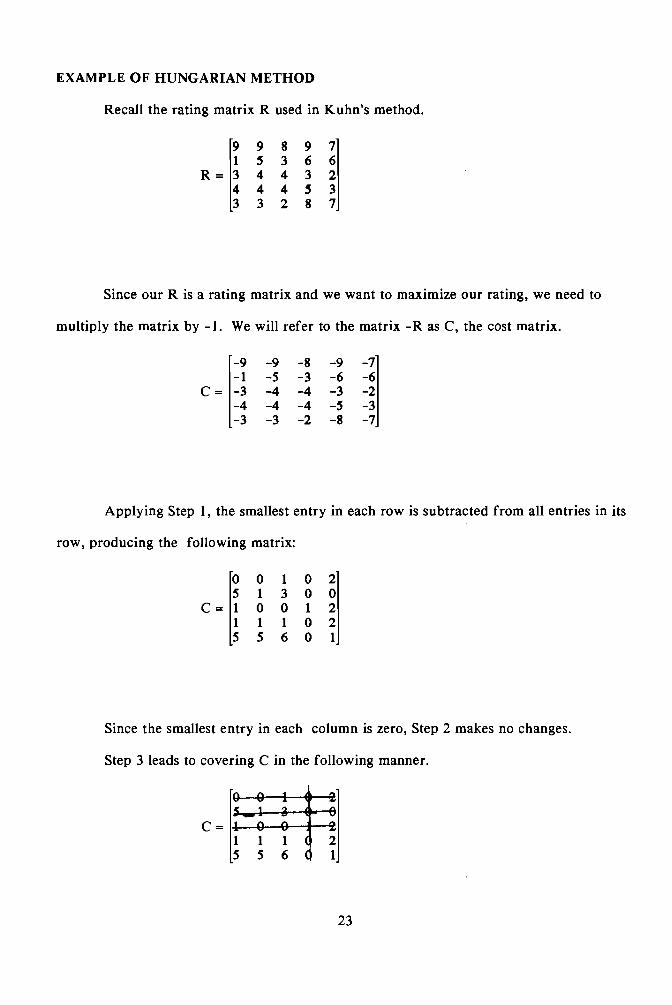
EXAMPLE OF HUNGARIAN METHOD
Recall the rating matrix R used in Kuhn's method.
9 9 897 1 536 6
R = 13 4 4 3 2 4 445 3 33287
Since our R is a rating matrix and we want to maximize our rating, we need to
multiply the matrix by -1. We will refer to the matrix -R as C, the cost matrix.
-9 -9 -8 -9 -7 -1 -5 -3 -6 -6
C = 1-3 -4 -4 -3 -2 -4 -4 -4 -5 -3 -3 -3 -2 -8 -7
Applying Step I, the smallest entry in each row is subtracted from all entries in its
row, producing the following matrix:
0 0 1 0 2 5 1 3 0 0
C = 11 0 0 1 2 1 1 1 0 2 5 5 6 0 1
Since the smallest entry in each column is zero, Step 2 makes no changes.
Step 3 leads to covering C in the following manner.
C = 11
23

Therefore the minimum number of lines needed is 4 which is less than n = 5. So
by Step 4, an optimal assignment can not yet be obtained. Hence, we apply Step 5. In
applying Step 5, the smallest uncovered entry, I, is subtracted from all uncovered entries
and added to all entries covered twice leading to the following C.
o o 1 1 2 5 131 o
C = 11 002 2 o 000 1 4 450 o
After Step 5, we return to Step 3. This time C is covered in this way.
6 8 1 1 2 S 1 3 1 9
C= 1,," 9 g 2 2 9 po 9 9 9 "\1 .. .. S 9 9
Step 4's test for optimality holds since the minimum number of lines needed was 5,
which is equal to n. Therefore, an optimal assignment is found, and we are done.
24
CHAPTER 4
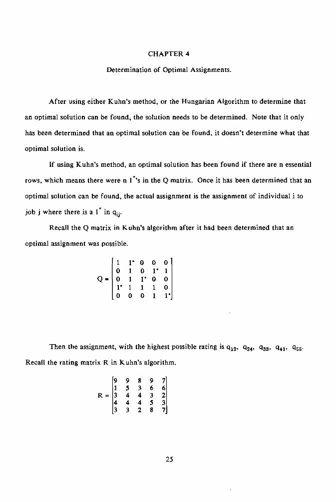
Determination of Optimal Assignments.
After using either Kuhn's method, or the Hungarian Algorithm to determine that
an optimal solution can be found, the solution needs to be determined. Note that it only
has been determined that an optimal solution can be found, it doesn't determine what that
optimal solution is.
If using Kuhn's method, an optimal solution has been found if there are n essential
rows, which means there were n I*,s in the Q matrix. Once it has been determined that an
optimal solution can be found, the actual assignment is the assignment of individual i to
job j where there is a I* in qij'
Recall the Q matrix in Kuhn's algorithm after it had been determined that an
optimal assignment was possible.
. 1 l' 0 0 0 0
Q= I0 1 1
0 l'
l' 0
1 0
l' 1 1 1 0 0 0 0 1 l'
Then the assignment, with the highest possible rating is ql2' q24' qgg, q41' q55'
Recall the rating matrix R in Kuhn's algorithm.
9 9 8 9 1 S 3 6
76
R = 13 4 3 24 4 4 4 S 3 3 3 2 8 7
25
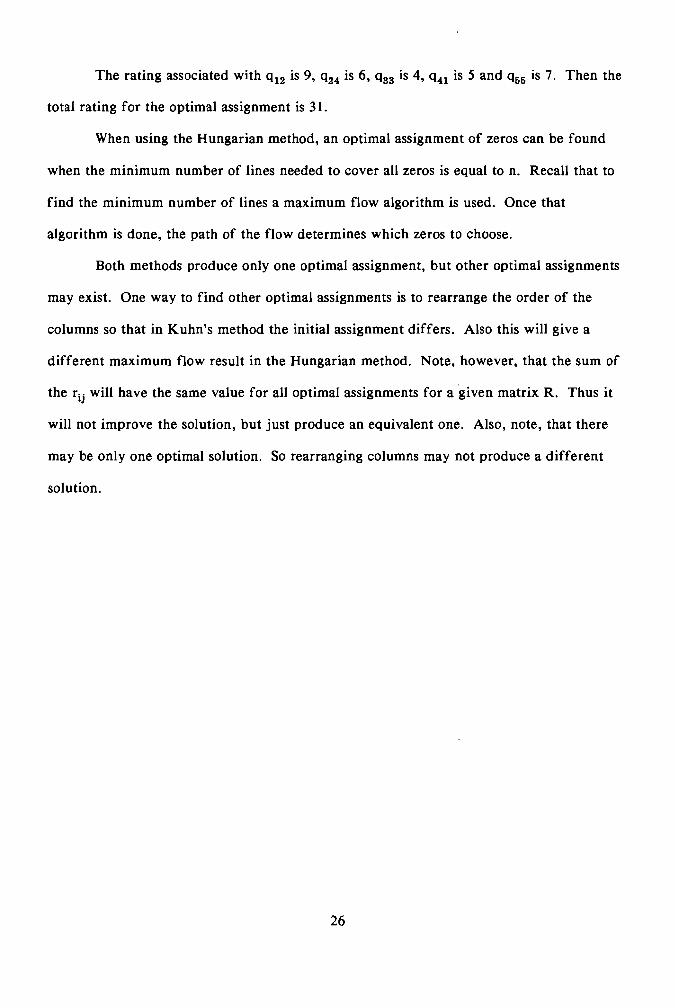
The rating associated with Q12 is 9, Q24 is 6, Qss is 4, Q41 is 5 and Q55 is 7. Then the
total rating for the optimal assignment is 31.
When using the Hungarian method, an optimal assignment of zeros can be found
when the minimum number of lines needed to cover all zeros is equal to n. Recall that to
find the minimum number of lines a maximum flow algorithm is used. Once that
algorithm is done, the path of the flow determines which zeros to choose.
Both methods produce only one optimal assignment, but other optimal assignments
may exist. One way to find other optimal assignments is to rearrange the order of the
columns so that in Kuhn's method the initial assignment differs. Also this will give a
different maximum flow result in the Hungarian method. Note, however, that the sum of
the rij will have the same value for all optimal assignments for a 'given matrix R. Thus it
will not improve the solution, but just produce an equivalent one. Also, note, that there
may be only one optimal solution. So rearranging columns may not produce a different
solution.
26

CHAPTER 5
Summary and Conclusion
While both the Hungarian method and Kuhn's algorithm are effective techniques
for solving the assignment problem, neither is trivial.
The Hungarian method requires finding the minimum number of lines needed to
cover all zero entries. If the matrix is small this may be an easy task, but relatively
speaking in any n x n matrix with n > 5, the task becomes difficult. In Kuhn's method the
task of checking the l's and l*'s needs to be performed efficiently. Much has been done
in the computer programming field to produce programs to alleviate the complexity of
each of these methods. [8, p.793]. Others have produced methods for speeding the process
in which an optimal solution can be found. [9, p. 194] The use of computer programs and
acceleration methods can greatly improve both the efficiency and the effectiveness of the
two methods.
Both of the methods require certain assumptions made. Of the assumptions Al - A3,
the only one that can be modified is AI, the number of jobs must equal the number of
individuals. If this assumption doesn't hold, for example, n jobs and n + 1 individuals, a
dummy job can be introduced into the matrix with a rating of 1 in Kuhn's method and a
cost larger than all other costs in the Hungarian method. then whichever individual was
assigned that job would not be assigned to any job.
The information on this topic is vast. The assignment problem has applications in
many other areas. In most introductory texts on linear programming the assignment
problem is addressed as a specific case of either the transportation problem, [6 p.490] or
the traveling salesman problem. [7, p.259] Usually when it is discussed, it is solved using
the Hungarian method instead of Kuhn's method. In the context of the traveling salesman
27

problem, usually found in introductory network theory texts, the covering of all zeros is
discussed as a maximum flow problem [7, p.323]. However, when the assignment problem
is presented in the context of the transportation problem the covering of zeros is not
thoroughly investigated. [6, p.491] The transportation problem is consistently found in
basic linear programming texts and the traveling salesman problem is usually found in
network Theory texts. In either case, the covering of zeros is never presumed to be a
trivial matter.
The assignment problem also is also treated in textbooks on operations research ego
[7, p.l12] and in systems analysis ego [7, p.114]. In order to study this subject further and
determine a more efficient algorithm for the assignment problem, further research in the
areas of network and graph theory would be essential.
28
Bibliography
1. Bazaraa, Jarvis, and Sherali, Linear Programming and Network Flows, New York, Wiley and Sons, 1990.
2. H.W. Kuhn, The Hungarian Method for the Assignment Problem, Naval Reasearch Logistics Quarterly 2, March-June(1956)712-726.
3. Rorres, Anton, Applications of Linear Algebra, Wiley and Sons, 1984.
4. G. Strang, Introduction to Applied Mathematics, Wellesly and Cambridge, 1986.
5. C. van de Panne, Linear programming and Related Techniques, North-Holland,1971.
6. E. Kaplan, Mathematical Programming and Games, New York, Wiley, 1982.
7. K. Mital, Optimization Methods in Operations Research and Systems Analysis, New York, Wiley, 1976
8. Glover, Karney, Klingman, and Napier, A Computation Study on Start Procedures. Basis Change Criteria, and Solution Algorithms for Transportation Problems, Management Science 20(1974),793-813.
9. V. Srinivasan, G.L. Thompson, Accelerated Algorithms for Laabel(ng and Relabeling of Trees. with Applications to Distribution Problems, Journal of the Assosciation for Computing Machinery, 19(1972),712-726

I
I, Laura J. Oliver , hereby submit this thesis/report to Emporia State University as partial fulfillment of the requirements for an advanced degree. I agree that the Library of the university may make it available for use in accordance with its regulations governing materials of this type. further agree that quoting, photocopying, or other reproduction of this document is allowed for private study, scholarship (including teaching) and research purposes of a nonprofit nature. No copying which involves potential financial gain will be allowed without written permission of the author.
~·-1;}-Date
The Optimal Assignment Problem Title of Thesis/Research Project
Date F"
Distribution: Director, William Allen White Library Graduate School Office Author