Embed Size (px)
Citation preview

ORES Working Paper Series
Number 111
The Out-of-Sample Performance of Stochastic Methods in Forecasting Age-Specific Mortality Rates
Javier Meseguer
July 2008
Social Security Administration Office of Retirement and Disability Policy
Office of Research, Evaluation, and Statistics
The author is with the Division of Economic Research, Office of Research, Evaluation, and Statistics, Office of Retirement and Disability Policy, Social Security Administration.
Working papers in this series are preliminary materials circulated for review and comment. The findings and conclusions expressed in them are the authors’ and do not necessarily represent the views of the Social Security Administration.
The working papers are available at http://www.socialsecurity.gov/policy. For additional copies, please e-mail [email protected].
Abstract
This paper evaluates the out-of-sample performance of two stochastic models used to forecast age-specific mortality rates: (1) the model proposed by Lee and Carter (1992); and (2) a set of univariate autoregressions linked together by a common residual covariance matrix (Denton, Feavor, and Spencer 2005). To this aim, death rates from 16 industrialized nations are used to compare observed ex-post mortality rates to the forecasts generated by the models. Several functions of the individual age-specific mortality rates are also entertained, including life expectancy at birth (e0), as well as alternative measures of the age-dependency ratio. The latter are constructed based on how the individual mortality rates enter a population projection, and thus, are meant to gauge the potential impact of mortality alone on public retirement programs. In general, both models are found to produce point forecasts for the individual mortality rates, life expectancy, and the dependency ratios that are fairly close to one another. Typically, the median projections of mortality moderately overpredict the actual death rates, particularly for the oldest age groups (ages 65–95 or older). Conversely, the large majority of the point forecasts of life expectancy at birth and the dependency ratios underestimate their observed values. The models also generate interval forecasts of e0 that are "too wide" as their empirical probability content often exceeds their nominal coverage. However, the Lee-Carter model tends to seriously underpredict the forecast uncertainty associated with both the death rates of the oldest ages and the age-dependency ratios, while the autoregressive approach overpredicts this uncertainty in most cases.

Introduction
Mortality is one of the key demographic variables affecting the flow of income and
expenditures in pay-as-you-go public retirement programs. Indeed, a combination of
population aging and declining fertility rates largely drives the currently projected
financial imbalance in the U.S. Social Security system. In recent years, official mortality
forecasts in a number of industrialized nations have come under greater scrutiny. The
deterministic nature of these projections and the role that expert judgment plays in
shaping them are often viewed by academics as sources of contention. Meanwhile,
demographers and other social scientists are increasingly turning to statistical time series
techniques to generate mortality forecasts that are consistent with a probabilistic
representation of uncertainty.
This paper will evaluate the performance of two alternative stochastic approaches that
can be applied to project age-specific mortality rates. Mortality data from 16
industrialized nations is used to carry out an extensive out-of-sample validation exercise
comparing actual mortality rates to the pseudo-forecasts generated by the models. This
analysis differs from other ex-post assessments published in the literature in two respects:
First, in addition to reporting several single-valued aggregate measures of performance, it
also investigates how forecast error is distributed across age groups and forecast
horizons. Second, this paper is not only concerned with a model's ability to produce
accurate point projections, but also with its capacity to generate a realistic depiction of
forecast uncertainty in terms of the empirical probability content of its interval forecasts.

2
The remainder of the paper is structured as follows: an introduction of the two models
that are the focus of the investigation; a description of the experimental design, followed
by the proposed ex-post validation exercise, and a discussion on the most salient features
of the mortality data used in the paper; a presentation on the out-of-sample performance
results; and the conclusion.
The Models
Stochastic forecasts are typically generated based on some underlying time-series
statistical model. This time series approach often involves a specified random disturbance
shock process, as well as a recursive expression that posits current values of the series in
question as a function of previous values. Once the model is fit to a particular data set and
estimates of its parameters obtained, future values of the series can be produced by
iterating the model forward. For simple models, the forecast distribution may be available
in closed-form. Otherwise, the researcher can turn to simulation by drawing from the
disturbance process to generate random sample paths of forthcoming observations. In
either case, the result is not only a single point forecast but an entire probability
distribution describing the uncertainty associated with future outcomes.
Modeling and projecting age-specific mortality rates over time is a high-dimensional
forecasting problem. Following the taxonomy suggested in Bell (1997), stochastic
projection models can be categorized as parametric or nonparametric, although this can
be a somewhat artificial distinction. The parametric or curve-fitting approach involves
fitting a curve defined by a finite set of time-varying parameters to the mortality data,
based on some optimization criterion. The resulting parameter estimates are then treated

3
as a time series that is projected to recover the different paths of the curve into the future
(that is, the mortality forecasts). The nonparametric approach relies on principal
components analysis to yield a linear transformation of the data, often in terms of an
approximation of reduced dimensions (one or a few principal components).
Stochastic projection methods can be further classified as univariate or multivariate
depending on whether the generated forecasts take into account the interdependencies
across the age groups. The former proceed by individually fitting each age-specific
mortality rate to a univariate time series equation. Although the forecasts produced by
univariate methods ignore the typically high cross-correlation among the different age
series, they do not necessarily perform worse than multivariate models. For instance, in
an ex-post validation experiment, Bell (1997) found that a random-walk with drift
applied to each age series led to better short-term forecast performance than any of a
variety of multivariate approaches. Nonetheless, there are several problems associated
with the univariate route. First, while the projections may be more accurate for each
individual age group, they can jointly imply unreasonable behavior. In particular,
univariate methods can lead to odd shapes in the fairly regular structure of mortality over
the entire age profile. Similarly, since this approach ignores the high degree of correlation
among the age series, it is unlikely to provide an accurate picture of overall forecast
uncertainty.
This paper focuses on the forecast performance of two models. First, the multivariate
nonparametric method proposed by Lee and Carter (1992). This model has gained
increasing recognition over the years, becoming a benchmark technique to the most
recent technical advisory panels to the Social Security Administration, the U.S. Census

4
Bureau, and several agencies around the world. The second model involves one of the
approaches suggested by Denton, Feaver, and Spencer (2005). This parametric model fits
first-order autoregressive processes to each age group separately. The resulting residuals
are then used to estimate the covariance matrix of the multivariate disturbance process
driving joint future variation in the age-specific mortality rates.
The Lee-Carter Model
The approach to mortality modeling proposed by Lee and Carter (1992) postulates the
logarithm of a set of age-specific mortality rates as the sum of a time-invariant age-
specific element and a second component that changes over time. Formally, let M
represent the A T× dimensional matrix of mortality rates with individual elements ,a tm
denoting the death rate for the population of individuals at age a and time .t Then,
,,log( ) a a t a ta t km β εα + += (1)
for 1, ,a A= … and 1, .t T= …
The age-specific set of parameters aα describes the average shape of the log-
mortality rates for every age category. The second component is the product of a time-
varying index or trend of the general level of mortality tk and a set of coefficients aβ
that determine both the direction and magnitude by which mortality at every age varies
with the index. Notice also that the parameters aβ and tk are not uniquely identified,
since for any given constant ,c an equivalent representation results by using /a cβ and
.tck Thus, Lee and Carter (1992) suggest imposing the following constraints:
0, 1.T A
t at a
k β= =∑ ∑ (2)

5
These constraints imply that the estimate of aα is simply the sample mean of the log-
mortality rates.
The Lee-Carter model represents a special case of the principal components (PC)
analysis applied by Bell and Monsell (1991) to forecast age-specific mortality rates.
Intuitively, PC analysis yields an approximation of the A age-specific mortality rates as
the linear combination of p "basic elements" or principal components estimated from the
data, where typically .p A≤ One way to compute the latter is via singular value
decomposition (SVD). Specifically, let M define the matrix of centered age profiles
obtained by subtracting the A sample logarithmic mortality means from the columns of
the matrix log( ).M The singular value decomposition of M yields a representation
involving the product of the following three matrices:
,M BLU ′= (3)
where L is a diagonal matrix with the singular values ordered from high to low, while B
is an orthonormal matrix whose first p columns correspond to the first p principal
components.1 The Lee-Carter model uses only the first principal component ( 1).p =
Therefore, the easiest way to estimate its parameters is by setting ˆaα to the sample mean
of the log-mortality rates, ˆaβ to the first column of B , and tk to the first row of ,LU ′
subject to the constraints in (2). These parameter values can be thought of as the least
square estimates resulting from minimizing the sum of squared errors function
( )2
,, ,
min log( ) .a a t
a t a a tk
at
m kα β
α β− −∑ (4)
1 Alternatively, the first p principal components can be defined as the eigenvectors corresponding to the
largest p eigenvalues of the product .MM ′

6
Once equation (1) is fitted to the data, the parameter estimates ˆaα and ˆaβ are taken to be
fixed, while the log mortality index tk provides a univariate time series whose future
values can be forecasted using standard Box-Jenkins techniques. In most applications, a
random-walk with drift is empirically found to yield a suitable fit to tk
21
ˆ ˆ , (0, ),t t t t ek k e e Nμ σ−= + + ∼ (5)
leading to the following maximum likelihood estimates for the drift and variance
parameters:2
( )1 2
211
1
ˆ ˆ 1 ˆ ˆˆ ˆ ˆ, .1 1
TT
e t tt
k kk k
T Tμ σ μ
−
+=
−= = − −− − ∑ (6)
Moreover, future values of tk can be obtained either analytically or via simulation, by
iterating equation (5) forward
1
ˆ ˆ ,h
T h T T ii
k k h eμ+ +=
= + +∑ (7)
where conditionally on the estimates 1 2ˆ ˆ ˆ, , , ,Tk k k… the usual mean forecast is a straight line
as a function of the forecast horizon ,h with slope μ
1 2ˆ ˆ ˆ ˆ ˆE | , , , .T h T Tk k k k k hμ+
⎡ ⎤ = +⎣ ⎦… (8)
It is then a simple matter to "plug" the projected values of the log-mortality index T hk +
back into equation (1) to recover the forecasts associated with each age-specific future
mortality
( ),
,
ˆˆlog( )
ˆˆexp .
a T h a a T h
a T h a a T h
m k
m k
α β
α β+ +
+ +
= +
= +
2 See for instance Girosi and King (2004; Chapter 2).

7
The Lee-Carter model yields a parsimonious stochastic approach to mortality
forecasting that is easy to implement and often produces reasonable forecasts for all-
cause age-specific mortality. The method, however, is not without its limitations. First, a
linear trend in the mortality index tk does not hold empirically in very long data sets. It
entails a constant geometric rate of decline for each age-specific mortality
,log( ).a t t
a
d m dk
dt dtβ= (9)
Yet, there is evidence that in a number of industrialized countries, the age pattern of
mortality decline over the past few decades has reversed (Lee and Miller; 2001). In
particular, the rapid decline in infant and child mortality characterizing the first half of
the twentieth century has diminished, with mortality decreasing faster for the elderly.
Furthermore, the Lee-Carter model implies that the rates of mortality decline for different
ages (for instance, 1a and 2a ) maintain a constant ratio to each other over time, regardless
of which univariate time series process is used to forecast tk :
1 1 1
2 2 2
,
,
log( ) / /.
log( ) / /a t a t a
a t a t a
d m dt dk dt
d m dt dk dt
β ββ β
= = (10)
As a result, the assumption of holding aβ constant over time seems unrealistic.
Finally, the Lee-Carter model incorporates uncertainty through a single source (the
sampling uncertainty derived from forecasting tk ). It is also possible to accommodate
additional uncertainty about the trend in mortality linked to the estimate of the drift
parameter ,μ as Lee and Carter (1992) originally discussed. However, this still ignores
uncertainty in the estimation of the aβ coefficients associated with ,tk as well as the error

8
from fitting the model using only the first principal component. Some demographers have
criticized the model’s interval forecasts as implausibly narrow.
Some Extensions of the Lee-Carter Model
There have been a number of refinements to the Lee-Carter specification. In fact, in their
original article, Lee and Carter (1992) addressed the two modifications considered in this
paper. In particular, the authors observed that the models’ forecasts do not match the
initial conditions in the jump-off year (that is, the forecasts are not linked to the actual
mortality rates at the end of the base period). One easy way to solve this problem is to set
aα equal to the most recently observed logarithmic age-specific rates, instead of their
time average. However, Lee and Carter (1992) caution that such an approach might
extrapolate features of mortality that are specific to the jump-off year and could have a
negative impact on model fit and forecast performance. In subsequent papers, Lee (2000)
and Lee and Miller (2002) seem to have reconsidered this position, favoring the modified
value of aα for forecasting purposes. Bell (1997), who also supports this bias correction
step, finds dramatic improvements in short-term out-of-sample forecast performance
when setting aα equal to the logarithm of the age-specific rates in the base year.3
Another improvement to the Lee-Carter model is concerned with the fact that the
OLS estimates of its parameters are the values minimizing error in the logarithm of the
death rates, rather than the death rates themselves. Consequently, the total number of
3 Notice that there are alternative ways to implement bias correction in the Lee-Carter model. For instance, Lee and Carter (1992) suggest setting the value of aα to the most recent rates prior to performing SVD,
while ignoring the normalization constraint on .tk By contrast, Lee (2000) favors estimating the model as
originally proposed, prior to changing .aα This paper follows the latter approach.

9
deaths predicted by the model is not guaranteed to match the observed death counts in the
sample. Lee and Carter (1992) propose a second stage reestimation of the mortality index
by holding ˆaα and ˆ
aβ fixed, while searching for a new estimate tk ∗ satisfying the
following equation
( ){ },ˆˆˆexp ,t a a t a t
a
D k Pα β ∗= +∑ (11)
where tD and ,a tP are respectively the total number of deaths and the population age a in
year .t Wilmoth (1993) suggests an alternative computational approach that estimates
,aα aβ , and tk simultaneously via weighted least squares, using the number of deaths at
each age as weights
( )2
,, ,min log( ) .a a t
at a t a a tkat
D m kα β
α β− −∑ (12)
The first model this paper entertains is a variant of Lee-Carter, incorporating the bias
corrections described in the previous paragraphs. Specifically, after some preliminary
experimentation, a decision was made to settle on the following estimation approach:
first, the model's parameters are computed by applying SVD on the matrix M of
centered logarithmic age profiles. Next, aα is set equal to the logarithm of the age-
specific rates corresponding to the last period in the sample. Finally, a second stage
reestimation of tk is performed to match total observed and fitted deaths.
A First-Order Autoregressive Approach
In a recent paper, Denton, Feaver, and Spencer (2005) suggest a number of multivariate
time-series econometric specifications as alternatives to the Lee-Carter method. One such

10
possibility is to model the first difference of logarithmic mortality
, , , 1log( ) log( ) log( )a t a t a tm m m −Δ = − as a th -p order autoregressive process AR ( )p :
, , ,1
log( ) log( ) .p
a t a sa a t s a ts
m c m eφ −=
Δ = + Δ +∑ (13)
Future changes in the individual mortality rates are determined by their own past values
plus a random disturbance term , .a te The age-specific series are estimated within a system
of seemingly unrelated regression equations (SURE) to accommodate the significant
contemporaneous correlation characterizing mortality data. Denton, Feavor, and Spencer
(2005) further suggest a second specification, which they refer to as a quasi-vector
autoregressive approach QVAR ( )p
, , ,1
log( ) log( ) log( ) ,p
a t a sa a t s sa t s a ts
m c m K eφ φ∗− −
=
⎡ ⎤Δ = + Δ + Δ +⎣ ⎦∑
where tK represents an index of mortality that is a function of all the individual age-
specific mortality rates, much like in the Lee-Carter model.
The second model this paper entertains is a variant of equation (13) with 1p = lags.
Formally, let ,a tm∗ denote the annual rate of improvement in mortality expressed as the
negative of the percent change in the central death rate:
, , 1,
, 1
100 .a t a ta t
a t
m mm
m−∗
−
−= − (14)

11
Each series is then fitted individually to a first-order univariate autoregressive AR(1)
model4
2, , 1 , ,, (0, ).a t a a a t a t a t em c m e e Nφ σ∗ ∗
−= + + ∼ (15)
Once parameter estimates ˆ ,ac aφ , and 2ˆeσ are computed, recursive substitution can
generate forecasts of future rates in mortality improvement by iterating equation (15)
forward
1 1
, , ,0 0
ˆ ˆ ˆˆ .h h
h i ia T h a a T a a a a T h i
i i
m m c eφ φ φ− −
∗ ∗+ + −
= =
= + +∑ ∑ (16)
The process ,a tm∗ can be shown to be covariance stationary if 1,aφ < with mean and
variance respectively equal to
2
22
, .1 1
a ea a
a a
c σμ σφ φ
= =− −
(17)
For a covariance stationary process, the mean h -step-ahead forecast, conditional on the
previous observations is given by
, ,1 ,2 , ,ˆˆ ˆE | , , , ( ),h
a T h a a a T a a a T am m m m mμ φ μ∗ ∗ ∗ ∗ ∗+⎡ ⎤ = + −⎣ ⎦… (18)
indicating that the projection decays geometrically from , ˆ( )a T am μ∗ − to the unconditional
estimated mean ˆ ,aμ as the forecast horizon h increases. However, since each individual
forecast ignores the typically high correlation among the age groups, the model is
modified to accommodate a joint disturbance process. In particular, the estimated
residuals ,ˆa te are used to compute the following covariance matrix
4 The Congressional Budget Office's stochastic model of Social Security's long-term trust fund finances uses a similar approach (CBO; 2000).

12
ˆ ,S S
T
′Ω = (19)
where each column of S corresponds to the residuals obtained from each equation.
Stochastic paths for the rates of mortality improvement are then generated by simulating
random shock vectors ˆ(0, )te N∼ Ω from the multivariate normal distribution.
Data and Experimental Design
The data sets used to carry out the ex-post validation exercise proposed in this paper were
obtained from the Human Mortality Database (HMD) and consist of mortality rates from
16 industrialized nations for males and females combined.5 Wilmoth (2004) documents
the methods by which the raw data were converted into mortality rates. The investigation
in this paper focuses on period death rates rather than cohort rates. In other words, the
mortality rates are indexed by year of occurrence rather than year of birth, so that ,a tm
denotes mortality at age a occurring in year ,t rather than the death rate of individuals
aged a born in year .t While analysis of rates on a cohort basis might be preferable, a
complete set of cohort mortalities requires a much longer time frame and can involve
significant missing data problems.
Formally, the period death rate ,a tm is defined as the ratio
,,
,
,a ta t
a t
Dm
E= (20)
5 The HMD is a collaborative project sponsored by the University of California at Berkeley and the Max Planck Institute for Demographic Research. The data, as well as both general and country specific documentation can be accessed via www.mortality.org or www.humanmortality.de.

13
where ,a tD is the death count for the population in the age range [ , 1)a a + on January
1st of calendar year ,t while ,a tE represents the exposure-to-risk (that is, the population
exposed to the risk of death), measured as total person-years lived in the same age
interval and time period. Generally, for a given country and year ,t death counts and
exposure-to-risk are available by single year of age from birth (age 0) to the open interval
110-years old and beyond (age 110 or older). Hence, to reduce the dimension of the
forecasting problem and reasonably fit the data to the stochastic projection models,
mortality rates were computed for the following 21 age groups: age 0, ages 1–4, ages
5–9,…, ages 90–94, ages 95 or older. The group rates were obtained by aggregating
single year of age values. For instance, the resulting death rate for the 1–4 age group at
time t was calculated as the ratio of total death counts for ages 1 through 4 over the sum
of exposure-to- risk values for the same ages and time period.
Ex-post validation analysis involves using an initial portion of the available data to
estimate a set of models that are then used to generate forecasts for the remaining time
period. This way, it is possible to compare the models' projections to the actual
observations to determine how well the models would have performed in the past. The
design of any ex-post validation experiment always requires somewhat arbitrary
decisions. For instance, the researcher must select the specific time frame and length over
which the behavior of the models should be investigated, the fraction of the data used for
estimation purposes, and the evaluation criteria employed to measure forecast
performance. The particular objectives of the analysis shape these decisions and constrain
the applicability of any conclusions. Table 1 lists the historical period of mortality data

14
available for each of the 16 countries.6 The shortest sample corresponds to the United
States (1959–2002) with 44 observations, while the longest sample belongs to Sweden
(1751–2003), with 253 observations.
This paper uses all available data regardless of potential country-specific concerns
about variation in quality, particularly when the estimated mortality rates date back more
than one century. This decision is justified by treating the selected stochastic models as
general algorithms, whose mechanically-generated forecasts should be tested under
multiple scenarios. Furthermore, to make the generated forecasts comparable across
countries, the initial jump-off year (the first period to be forecast) is fixed to 1980 in all
cases. This particular choice was made based on the shortest available data set, by
roughly adhering to two guiding principles: First, for each series there should be at least
as many in-sample observations as the length of the forecast horizon. Second, the
estimation sample per series should be at least as large as the total number of variables to
be projected (21 age groups).
To minimize the impact of the selected jump-off year on the resulting projections, it
is common practice in out-of-sample validation exercises to focus on the forecast error
corresponding to fixed lead times, using different forecast origins. In other words, for
every country, each model is fitted using all observations from the beginning of the series
until 1979 and mortality projections generated from 1980 to the end of the data set. Then,
the sample is expanded to include the next observation (1980). Upon reestimation, new
forecasts are generated from 1981 to the end of the series. This process is repeated until 6 The mortality rates corresponding to Germany were obtained by pooling the death counts and risk-to-exposure estimates listed separately for East and West Germany in the HMD. The U.K. data comprises England and Wales.

15
the only period left to forecast is the last available observation. For instance, for each age
group in the United States, , the projections generated over the various jump-off years
(1980, 1981,…, 2001) yield a set of 23 forecasts involving a 1-year horizon, 22 forecasts
involving a 2-year period, and eventually a single forecast 23 years ahead. The fourth
column of Table 1 shows the size of the longest forecast horizon (from 1980 to the end of
each series). By design, the analysis centers on evaluating forecast performance over the
short– to medium-range (23 to 25-year horizons in most cases), a fact that is determined
by the choice of initial jump-off year, given the small sample sizes of some of the data.
The last column in Table 1 presents the total number of projected observations per age
group, over all forecast horizons.
Chart 1 displays three-dimensional surfaces, as well as contours of the logarithmic
age profile of mortality corresponding to the United States and the United Kingdom.
They serve to illustrate a number of features in all-cause mortality common to most
nations. One characteristic of the data is the regularity in the shape of mortality over the
ages. For any given period, mortality declines smoothly from birth until about ages 10–
14, then increases almost linearly for the remaining ages until death. Moreover, in the
second half of the twentieth century, the death rates experience a sharp increase
associated with motor-vehicle fatalities in the 15–19 age group, often referred to as "the
accident hump." Notice also how the surface for the United Kingdom appears far less
smooth than the one corresponding to the United States. The former contains a much
longer data sample (1841–2003) that includes spikes in mortality associated with the two
world wars and the 1918 Spanish influenza pandemic.

16
When modeling mortality, some researchers treat unusual data spikes as outliers by
introducing dummy variables to remove their influence. An alternative view is that these
observations represent rare but nonetheless potentially recurring shocks, and thus, their
exclusion is likely to underestimate true uncertainty. The analysis in this paper subscribes
to the latter practice, treating all observations equally. Yet a third possibility, as Lee and
Carter (2000) suggest, is to incorporate additional uncertainty in every forecast period
due to such events. For example, this can be accomplished by introducing a 1/( 1)T −
chance of a shock to the mortality index tk the size of the 1918 influenza pandemic,
where T denotes the sample size. Nevertheless, the authors report that this practice has a
negligible effect in the resulting projections.
A second characteristic in the age profile of all-cause mortality is a downward trend.
That is, while mortality across the age groups maintains its regular shape, it also shifts
downward over time. This can be clearly seen in the bottom graphs of Chart 1, which
show the logarithm of the age mortality profile at three different points in time for the
same two countries. It is evident that the death rates among the various age groups tend to
move together. Thus, it is not surprising that a third feature of all-cause mortality
involves a high degree of cross-correlation among the rates for different ages.
Table 2 presents the sample correlation between each age series and its immediately
adjacent group for all 16 countries. For instance, the top entry in the column of Table 2
corresponding to Austria indicates that the estimated correlation between the age 0 and
age 1–4 groups is 0.988. Similarly, the correlation between age groups 90–94 and 95 or
older is 0.748 (the last entry in the same column). Evidently, mortality across the ages

17
shows a high degree of positive association. Finally, Table 3 shows the sample standard
deviation of the mortality rates corresponding to several age groups. Clearly, there is
much more variation in mortality within the older age groups (particularly for the last
series age 95 or older), as well as before age 1. Typically, the standard deviation
decreases rapidly from a relatively high value at birth (age 0), until it reaches the 10–14
age group. Then, it increases steadily from ages 15–19 to the last series (age 95 or older),
where it often attains its highest value.
Before turning to the ex-post validation results presented in the next section, it is
important to discuss a number of findings in the literature that are relevant to this paper.
Denton, Feavor, and Spencer (2005) use Canadian mortality data from 1926 to 2000 to
produce long-term forecasts of life expectancy at birth and ages 65 and 80, based on the
specification in equation (13) with 2p = lags. The authors utilize a partially parametric
method to generate random variation via a bootstrap procedure. They also implement a
fully parametric approach by drawing from a multivariate normal disturbance process,
much like the second model entertained in this paper. Although Denton, Feaver, and
Spencer (2005) do not conduct an analysis of the out-of-sample forecast performance of
these models, they do find the point forecasts generated by the fully parametric approach
much closer to the projections of the Lee-Carter method than the official forecasts of the
Canada Pension Plan.
Lee and Miller’s (2001) ex-post validation analysis also focuses on life expectancy at
birth 0 ,e comparing actual and hypothetical forecast errors in the Lee-Carter model with

18
those of the Social Security Administration (SSA).7 Using U.S. data from 1900 to 1998
(with 1921 as the initial jump-off year), the authors find that the empirical distribution of
the actual forecast error matches well its hypothetical counterpart within a 10-year
period, but deteriorates over time. Generally, the Lee-Carter model tends to underpredict
life expectancy, although not by as much as the official SSA projections. In addition, the
interval forecasts of 0e appear to be "too wide" up to the first 50 forecast horizons, while
underestimating their hypothetical probability content for longer periods. Lee and Miller
(2001) reach similar conclusions in more limited pseudo-forecast experiments using data
from Japan, Canada, France, and Sweden.
Finally, Bell (1997) implements an evaluation of the short-term out-of-sample
forecast behavior of multiple models using U.S. central death rates for white males and
females from 1940 to 1991 (with 1981 as the initial jump-off year). Unlike Lee and
Miller (2001), Bell reports forecast error over the entire age profile instead of relying on
life expectancy as a single-valued measure of forecast performance. He finds that a
univariate random-walk with drift fitted separately to each age group outperforms all of
the parametric and nonparametric multivariate approaches considered. Only the Lee-
Carter model with the type of bias correction discussed previously yields a similar
forecast error to the univariate approach.
Out-of-Sample Forecast Performance
As previously mentioned, ex-post validation analysis provides a means to determine how
well a set of models would have performed in the past, by comparing the forecasts 7 Notice that Lee and Miller (2001) employ a different variation in the second stage estimation of ,tk
matching life expectancy for that year instead of total number of deaths.

19
generated by the models to the actual observations. This kind of analysis is not without its
limitations, and should not be confused with forecasts that are generated in real time. The
latter are produced prior to the forecast period, when the future outcome is truly
uncertain. The former enjoy the advantage of perfect foresight, and are therefore based on
an information set that was not available during the forecast period. Keeping these
drawbacks in mind, ex-post validation is still a very valuable tool that cannot be replaced
by in-sample goodness-of-fit measures. In particular, ex-post validation provides answers
to "what if" type scenarios that are useful in specifying and calibrating models to be used
for real time forecasting.
To compare forecast performance among several models, the following elements
must be specified a priori: (1) the variables of interest to be projected; (2) the estimators
used to measure these variables; and (3) an appropriate criterion to evaluate the variables’
forecast performance. Clearly, with respect to the first point, the ultimate object of
investigation is the 21 different age-specific mortality rates being modeled
simultaneously. This paper looks at both the accuracy of the point projections produced
by the models, and the ability of these projections to provide a realistic representation of
forecast uncertainty. The means and medians of the generated forecast distributions are
presented as two alternative point estimators. On the other hand, the capacity of the
models to gauge forecast uncertainty is assessed by the behavior of their interval
projections. To this aim, 90-percent confidence interval forecasts are also estimated using
the 5th and 95th quantiles of the resulting forecast distributions.
The performance of the point estimates is evaluated using the traditional root mean
squared error (RMSE) measure. Conversely, the performance of the interval projections

20
is determined in terms of their empirical probability content (that is, the fraction of times
the generated intervals actually include the observed ex-post mortality rates). If the
interval forecasts enjoy an empirical probability content that is close to its hypothetical
90 percent level, it is likely that the model does a good job at accommodating the
uncertainty associated with its point projections and can be used reliably for inference.
However, coverage alone is only part of the picture. Since by design a fixed forecast
interval between 0 and 1 covers the entire sample space, it is guaranteed to contain the
ex-post mortality rates 100 percent of the time. Yet, such an interval has no practical use
for inference, as it does not convey any information not already known a priori. Hence,
the average width of the generated forecast intervals is also reported. Clearly, one
unequivocal way to rank the interval estimates generated by several models involves the
trade-off between probability coverage and interval width. In particular, an interval
forecast that is narrower than all others and also enjoys greater empirical coverage should
be the preferred choice.
Typically, when comparing multivariate forecast models, it is unusual for one model
to outperform all others for every series projected at every forecast horizon. This is
particularly likely in this application, given both the relatively large number of data sets
and variables (21 age-specific mortality series for each of 16 samples). Therefore, to
evaluate overall model performance, it is useful to adopt a single-valued measure that
combines all the variables. One quantity to consider is life expectancy at birth 0, ,te
defined as the average number of remaining years an individual born at time t is

21
expected to live. Following the discussion in Wilmoth (2004), let ,a tl denote the number
of survivors at age a in year t
1
, 0, ,0
(1 ),a
a t t i ti
l l m−
=
= −∏ (21)
out of an initial population arbitrarily set to 0, 100,000,tl = for 1, , .a A= … The person-
years lived in the age interval [ , 1)a a + is given by
, , , , ,(1 ) ,a t a t a t a t a tL l w l m= − − (22)
with ,a tw representing the average number of years lived within the age interval.8 Then,
period life expectancy at birth is defined as follows
0,0,
0,
,tt
t
Te
l= (23)
where 0, tT denotes the person-years remaining at birth
0, ,0
.A
t a ta
T L=
=∑ (24)
Evidently, life expectancy at birth is a highly nonlinear function of all of the age-
specific mortality rates that carries a natural interpretation. For this reason, it is often
reported in practice as an overall summary measure of forecast performance, as in Lee
and Miller’s (2001) ex-post analysis. Unfortunately, such an aggregate quantity can be
deceiving in that the forecast error associated with individual age groups could
8 For single-year ages except age 0, ,a tw is usually set to one-half, under the assumption that deaths occur
uniformly. In addition, notice that for period life table calculations, the mortality rates ,a tm are transformed
into probabilities of death ,a tq using standard procedures.

22
potentially cancel each other out in the computation of person-years remaining at birth,
masking the extent of the forecast error experienced at particular ages.
Bell (1997) uses an alternative gauge of overall performance that looks at forecast
error over the entire age profile. For instance, for the point projections, the RMSE
corresponding to a particular forecast horizon is computed by averaging over the squared
difference of observed and projected mortality at every age. This kind of measure is
typical in multivariate time-series econometric applications. While not nearly as intuitive
in its interpretation as life expectancy, it does not suffer from the potential problem that
the forecast errors at different ages might cancel each other out. However, the measure is
not without its drawbacks. In particular, suppose that a few of the series experience error
that is disproportionately high relative to the remaining ages. Then, those few groups will
largely determine the resulting total forecast error. A more robust measure of forecast
error in the age profile might entail using a weighted average, with weights determined
by the sample precision of each age series (that is, the inverse of its sample standard
deviation). This more robust measure would define the importance of the error
contributed by every age group as a function of how much variation mortality at that age
displays in the sample, relative to the remaining series. Nevertheless, for the purposes of
the forthcoming analysis, equal weights are assumed throughout.
In addition to both life expectancy at birth and the entire age profile as overall
measures of forecast performance, the impact that mortality has on the program's future
finances is an even more relevant criterion for a pay-as-you-go pension system. This
impact is typically defined by the age distribution of the population, in terms of the old-
age dependency ratio (the ratio of retired to working age population). Of course, to

23
generate population forecasts, we would also need to model fertility and net migration,
which is outside the scope of this paper. Nonetheless, it is still possible to evaluate the
manner in which the age-specific mortality rates would actually enter into a population
projection of the old-age dependency ratio, and thus, measure the effect that the mortality
projections alone have on the program's finances. Specifically, recalling the previously
defined number of survivors ,a tl at age a in equation (21), the following dependency
ratios implied by the individual age mortality rates are entertained:
95
,651, 64
,20
,i ti
t
i ti
l
lδ
+
=
=
= ∑∑
(25)
95 19
, ,65 02, 64
,20
.i t i ti i
t
i ti
l l
lδ
+
= =
=
+= ∑ ∑
∑ (26)
At a given point in time ,t 1, tδ refers to the ratio of survivors at ages 65 or older over
those ages 20 to 64. Alternatively, 2,tδ embodies a more general measure of dependency
encompassing both the youngest and oldest ages in the numerator (from birth to age 19,
as well as ages 65 or older).
For the purpose of illustration, Charts 2 through 4 display a number of projections
generated at the initial jump-off year using the mortality data for the United States and
United Kingdom. The top graphs in Chart 2 show actual mortality for the 10–14 age
group, along with the median and 90-percent interval forecasts generated by the models
from 1980 to the end of each series. The bottom graphs display forecasts corresponding
to the 70–74 age group. The top of Chart 3 presents similar projections of life expectancy
at birth, while the bottom graphs illustrate different measures of the dependency ratios

24
defined above. In particular, the thickest solid lines in the bottom part of Chart 3
respectively represent the historical values of 1, tδ and 2, ,tδ based on the actual population
figures from the Human Mortality Database. For instance, for the United States, the
dependency ratios in the year 2000 were 1, 0.212tδ = and 2, 0.698.tδ = 9 By contrast, the
remaining lines in the same graphs represent the dependency ratios based on the mortality
rates alone, abstracting from fertility and net migration. These are the quantities relevant
to the ex-post analysis in this paper. Their values for the United States in 2000 were
1, 0.351tδ = and 2, 0.817.tδ = Chart 4 shows projections of these two dependency measures.
The experimental design of the ex-post analysis implemented in this paper looks at
forecast error at fixed lead times, using different forecast origins. For every data set and
model, 20,000N = random paths are simulated from 1980 forward for each of the 21 age
groups. Since the Lee-Carter model takes as inputs the logarithmic death rates while the
AR(1) approach models the rates of mortality improvement, the generated paths are
transformed back into mortality rates prior to computing the features of interest of the
forecast distribution. The mortality paths are then used to calculate the mean, median, and
5th and 95th quantiles for each age group and forecast period. In addition, the simulations
corresponding to all 21 ages are also used to compute similar estimates for life
expectancy at birth 0, te and the dependency ratios 1, tδ and 2, .tδ Finally, the same process
is repeated with other jump-off years (1981, 1982, 1983 and so on). This is done to limit
the influence of any particular forecast origin on the results, and thus, improve the
9 For comparison, the corresponding values reported in Table V.A2 of the 2005 Trustees Report, based on the total Social Security area population at mid-year in 2000 are respectively 1, 0.208tδ = and
2, 0.693.tδ =

25
robustness of the findings. At the end of the exercise, there are n projections of the
quantities of interest with a 1-year forecast horizon, 1n − projections 2 years ahead, and
eventually, 1 projection n years into the future, where n denotes the longest forecast
horizon available, as the fourth column of Table 1 shows.
Once all the projections are obtained it is a simple matter to evaluate forecast error
using the specified performance criteria. For the point estimators (means and medians),
performance is measured in terms of RMSE. Formally, let , ,ˆ a t tm Δ represent the tΔ -step-
ahead forecast of the mortality rate for age group a in year .t The RMSE associated with
a particular age series and fixed lead time tΔ is calculated as follows:
( )2
, , , ,
1ˆRMSE ,
1i
T
a t a t t a tt ti
m mT tΔ Δ
=
= −− + ∑ (27)
where it represents the jump-off year of the forecast in question and ,a tm denotes
observed mortality. For instance, taking a 1-year forecast horizon ( 1),tΔ = for the United
States (see Table 1) there are 23 forecasts spanning the period from 1980it = to 2002.T =
Similarly, there are 14 ten-step-ahead forecasts ( 10),tΔ = with 1989it = and 2002,T =
while the single 23-years-ahead projection involves 2002it T= = .
The performance of the interval forecasts is determined by computing the actual
fraction of times ex-post mortality rates lie inside the intervals. Let , ,ˆ
a t tC Δ denote the area
covered by the 90 percent tΔ -step-ahead interval forecast of mortality for age-group a in
year .t Furthermore, define an indicator function taking a value of 1 if the calculated
, ,ˆ
a t tC Δ includes the observed mortality rate, and 0 otherwise:

26
( ), , ,
, , ,
ˆ1 if ˆ, .
0 otherwise
a t a t t
a t a t t
m C
I m CΔ
Δ
⎧ ∈⎪
= ⎨⎪⎩
(28)
Then, the empirical probability associated with the interval projection at age a and
forecast horizon tΔ is given by
( ), , , ,
1 ˆ, .1
i
T
a t a t a t tt ti
P I m CT tΔ Δ
=
=− + ∑ (29)
A similar approach is used to calculate the average width of the intervals.
Finally, the overall measures of performance are a function of either all or most of the
21 age groups. In this case, the forecast error associated with the point estimates of the
entire age profile at a particular forecast horizon tΔ is simply obtained by averaging over
the ages
( )2
, , ,1
1 1ˆRMSE .
1i
A T
t a t t a ta t ti
m mA T tΔ Δ
= =
= −− +∑ ∑ (30)
Likewise, the RMSE associated with, for instance, the point projections of life
expectancy at birth and forecast horizon tΔ is computed as follows
( )0
2
, 0, , 0,
1ˆRMSE .
1i
T
e t t t tt ti
e eT tΔ Δ
=
= −− + ∑ (0.1)
Similar expressions for the dependency ratios are obtained by replacing 0, ,ˆ t te Δ and 0, te
above with the corresponding values of , ,i t tδ Δ and ,i tδ . The extension of these equations to
compute the empirical coverage and average width of the interval estimates is also
obvious. In addition, it is straightforward to modify these expressions to estimate forecast
error over multiple forecast horizons or the entire forecast period.

27
Forecast Performance of Point Projections
The first four columns of Table 4 present the resulting RMSE corresponding to the
median forecasts of the Lee-Carter (LC) model for the following measures of overall
forecast performance: the age profile, life expectancy at birth 0e , and the two age-
dependency ratios 1δ and 2δ defined in equations (25) and (26), respectively. These
quantities are computed over all available forecast horizons. Since both the means and
medians of the forecast distribution are entertained as plausible point estimators, columns
5 through 8 in Table 4 display the ratio of RMSE between the two. Clearly, for the first
three measures (the age profile, 0e , and 1δ ), the median is a better performing point
estimator than the mean in the large majority of cases, as most of the ratios exceed 1.
Only for the more comprehensive measure of dependency 2( )δ do the mean projections
generally exhibit lower RMSE than their median counterpart, although the differences
between the two are fairly small. Moreover, while not shown for the sake of conciseness,
the results corresponding to the AR(1) model are qualitatively similar. In light of these
findings, this paper focuses exclusively on the median forecasts from this point forward.
To facilitate comparison, columns 1 through 4 in Table 5 present the ratios of RMSE
in the median forecasts between the LC and AR(1) models (again, over all forecast
horizons). Notice how forecast performance can vary across the different specified
criteria. For example, for the Netherlands or the United States, the AR(1) approach
outperforms Lee-Carter over the age profile, while the latter model actually exhibits
lower RMSE for the projections of life expectancy and the dependency ratios.
Conversely, for Finland, Germany and Japan, the LC model enjoys lower RMSE over the

28
age profile but is outranked by the first-order autoregressive approach in the remaining
measures.
The LC model outranks the autoregressive approach in half of all cases for 1δ and the
age profile, while the AR(1) model displays lower RMSE in the other half. For life
expectancy at birth 0 ,e the LC model does better in 7 of the data sets but is outperformed
in the remaining 9 cases. For the broader dependency measure 2 ,δ the AR(1) approach
outperforms the LC model in 11 out of the 16 countries. Furthermore, in most instances,
the differences in performance between the models are relatively small (that is, most of
the ratios are fairly close to 1). There are a few notable exceptions to this finding for the
forecasts of 0.e For instance, for France, the AR(1) approach reduces forecast error in life
expectancy at birth by almost half relative to the LC model—likewise for the Netherlands
and the United States. Overall, however, both models seem to display rather similar
performance.
The remaining columns in Table 5 report the percentage of times the median
projections in both models fall below the actual values for each of the four evaluation
criteria. Clearly, for a given measure, the percentages corresponding to each model are
very close to one another, suggesting that both models generate forecasts that are roughly
biased in the same direction. With the exceptions of Japan, Spain, and the United States,
notice that over the age profile, the percentages in Table 5 fall below 50 percent, so that
the models tend to moderately overestimate actual mortality in most cases. By contrast,
the large majority of the forecasts of life expectancy at birth and the age-dependency
ratios underestimate their observed values. Specifically, only the median projections

29
corresponding to Japan and the United States overpredict life expectancy, while the
dependency ratios are also overestimated only for the United States. For the remaining
data sets, between 70 percent to 99 percent of all generated forecasts underpredict 0 ,e 1δ ,
and 2.δ
To gain insight into the results presented in Table 5 (the models' forecasts
overestimate actual mortality but underestimate life expectancy and the age dependency
ratios), it is important to consider the mechanism via which the age-specific mortalities
enter the calculation of 0 ,e 1δ , and 2.δ In all cases, the quantities that matter are the
longitudinal numbers of survivors out of some initial population, as defined in equation
(21). Suppose that a particular forecast ,ˆ a tm overpredicts actual mortality at age a and
time .t Then, the implied survival rate , ,ˆ ˆ(1 )a t a ts m= − will underestimate the projected
number of people that graduate into the next age category. Of course, whether the
resulting future estimates of life expectancy at birth will underproject the observed values
depends not only on the fraction of the age-specific rates that overestimate mortality, but
also on the magnitude of their forecast error. Dependency ratios are further complicated
by the fact that they comprise the quotient of longitudinal numbers of survivors at
different ages, so that the distribution of both the bias and magnitude of forecast error
across the ages plays a large role.
Performance by Age Group
One way to measure how error is distributed among the ages is to determine the
percentage that each particular age group contributes to the value of total forecast error.
For ease of presentation and to maintain consistency with how the dependency ratios

30
have been defined, the individual age groups are aggregated into three broad categories
(ages 0–19, ages 20–64, and ages 65–95 or older, respectively), containing 5, 9, and 7 of
the 21 original groups. Broadly, these three categories encompass birth to young
adulthood, the working population, and individuals in retirement ages. Following the
discussion in the previous section, the RMSE associated with some individual age group
a over all forecast horizons tΔ is determined by
( )2
, , ,1
1 1ˆRMSE ,
1i
n T
a a t t a tt t ti
m mn T t Δ
Δ = =
= −− +∑ ∑ (32)
where n denotes the longest forecast horizon shown in Table 1. Similarly, the
computation of RMSE over the entire age profile involves
( )
( ) ( ) ( )
2
1
2 2 2
1RMSE RMSE
RMSE RMSE RMSE ,j j
A
aa
a aa a a a
A
A
=
∈ ∉
=
= +
∑
∑ ∑
with ja representing either a single age group or a subset of ages, such as the 65–95 or
older retirement category. It follows then, that the proportion ip of total mean squared
error (MSE) corresponding to ja is given by
( )
( )( )
( )
2 2
2 2
RMSE RMSE1 .
RMSE RMSE
a aa a a aj jip
A A
∈ ∉= = −∑ ∑
(33)
Table 6 displays the percentage of forecast error over the entire age profile that is
attributed to two broad sets of ages. The first set comprises the initial 14 age groups being
modeled (from birth to age 64). These series make up less than 1 percent of total forecast
error in most cases, and less than 3 percent in both models and all 16 data sets. By
contrast, the retirement ages account for 97 percent to 99 percent of total MSE. In terms

31
of model performance by age, the first three columns in Table 7 present the ratio of
RMSE between models for the three broad age categories specified by the dependency
measures. The first-order autoregressive approach outperforms the Lee-Carter model in
11 out of the 16 countries for the youngest age groups (ages 0–19), 7 countries for the
working population (ages 20–64), and half of all countries for the retirement category
(ages 65–95 or older). Furthermore, a comparison of the ratios in the first column of
Table 5 with those in the third column of Table 7 reveals that they are virtually identical
in magnitude, confirming once more that the oldest age groups overwhelmingly
determine total forecast error over the age profile. The remaining columns in Table 7
show the percentage of the median forecasts that fall below the observed ex-post
mortality rates by model and broad age category. Clearly, in all but one case (the United
States), the models are far more likely to overestimate actual mortality for the oldest ages
than for any age group. In most cases, over three-fourths of the generated projections for
the 65–95 or older ages overpredict observed mortality.
Two obvious patterns concerning the models' median forecasts emerge from Tables 6
and 7. First, the bulk of forecast error is heavily concentrated among the oldest ages.
Second, the majority of the forecasts corresponding to these age groups overestimate
observed mortality. These findings shed additional light on the results shown previously
in Table 5. In particular, a very high proportion of the forecasts for the 65–95 or older age
groups overestimates mortality and hence, underestimates the number of population
survivors at these ages. Furthermore, since these groups carry greater importance in
determining how the magnitude of the forecast error is distributed across the ages, they
are more likely to underpredict the total number of person-years remaining at birth, and

32
thus 0.e Similarly, the 65–95 or older age groups enter the computation of the
dependency ratios through the numerator. Consequently, if the number of survivors at
these ages is underestimated, so are likely to be the values of 1δ and 2.δ The exception to
this pattern involves the projections for the United States, where mortality is
underestimated at the oldest ages instead, while the forecasts of life expectancy and the
dependency ratios overestimate their ex-post values.
Performance by Forecast Horizon
To assess how the median forecasts change with the length of the forecast horizon, the
generated projections are grouped into four periods: 1–5 years, 6–10 years, 11–15 years,
and 16 or more years ahead. Notice that the last category varies with the final year of data
available for each series, involving 16–23 years ahead in most cases. Table 8 presents the
ratio of RMSE between models over the age profile, as well as the percentage of the
median forecasts that fall below observed ex-post mortality over the various forecast
horizons. Tables 9 through 11 display similar quantities for the projections of life
expectancy at birth 0e and the dependency ratios 1δ and 2 ,δ respectively. Although not
discernible from the ratios in the first four columns of each table, as expected, forecast
error generally increases with the distance of the forecast horizon.
Beginning with the age profile in Table 8, the first-order autoregressive approach
outperforms the Lee-Carter model in ten cases for the 1–5 and 11–15 year horizons and
in eight cases for the 6–10 and 16 or more year periods. While not always true, the
differences in model performance tend to increase with the length of the forecast horizon,
with the largest divergence corresponding to Austria in the 16 or more year period, where

33
RMSE over the age profile for the AR(1) model is approximately 25 percent greater than
for the LC approach. In most cases, a moderately larger proportion of the mortality
forecasts tend to overpredict their observed values, except for Japan, where roughly
three-fourths of the mortality forecasts involve underpredictions. The same pattern holds
true for Spain and the United States, where approximately 50 percent of all forecasts
underpredict mortality. Moreover, in about half of all countries, the percentage of
projections overpredicting mortality increases as a function of the forecast horizon.
Turning to the median projections of life expectancy at birth in Table 9, the LC model
outperforms the AR(1) approach in thirteen countries for the 1–5 year horizon, nine
countries for the 6–10 year period, eight countries for the 11–15 horizon, and seven
countries for 16 or more years ahead. Barring a few exceptions typically involving the
longest forecast horizons (such as France, the Netherlands, and the United States), most
of these ratios are relatively close to 1. Moreover, excluding the United States and Japan,
the projections generated by both models overwhelmingly underpredict life expectancy,
particularly as the distance of the forecast horizon increases. In fact, at the 16 or more
year horizon 100 percent of the forecasts of life expectancy at birth underpredict their ex-
post values for the majority of the data sets in both models.
Finally, Tables 10 and 11 show the performance of the point projections of the
dependency ratios. For the 1δ ratio (survivors at ages 65–95 or older over ages 20–64),
the LC model outperforms the AR(1) approach in ten cases for the 1–5 and 6–10 year
horizons, nine cases for the 11–15 year period and eight cases for 16 or more years ahead.
On the other hand, for the broader measure of dependency 2δ (ages 0–19 and 65–95 or

34
older over 20–64), the LC approach outranks the autoregressive model in ten cases for
the 1–5 year forecast period, six cases for the 6–10 year horizon, and only five cases for
11–15 and 16 or more years ahead. For both measures of dependency and all sixteen data
sets, the largest difference in performance between the models does not exceed 26
percent at any forecast horizon. In all but one instance (the United States), the median
projections of both dependency ratios underestimate their observed values increasingly as
a function of the forecast period. At the 16 or more year horizon, virtually all of the
generated forecasts underestimate the observed dependency values, while the converse is
also true for the U.S. data (none of the median projections fall below the corresponding
ex-post quantities).
Forecast Performance of Interval Projections
The first two columns in Table 12 display the empirical probability content of the 90-
percent forecast confidence intervals generated by the models for the age profile, over all
forecast horizons. The third and fourth columns in the same table respectively present the
average width of these intervals for the Lee-Carter model, and the ratio of average width
between models. The last four columns in Table 12 show similar quantities for life
expectancy at birth 0 ,e while Table 13 displays analogous coverage and width measures
for the two age dependency ratios 1δ and 2.δ
Beginning with the age profile, it is evident that over all the age groups, the first-
order autoregressive approach yields interval projections in every single case that exhibit
greater probability content than the Lee-Carter model, but are also much wider. In
general, the LC model seems more likely to generate mortality intervals that are "too

35
narrow" (that is., that fall below their nominal 90-percent level of coverage). Conversely,
the AR(1) model tends to produce intervals that are "too wide." For instance, with the LC
model, only 4 nations exhibit coverage greater than or equal to 90 percent (France, the
Netherlands, Sweden, and Switzerland), while in 9 of the 16 cases empirical coverage
falls below 80 percent. By contrast, with the first-order autoregressive approach,
probability content is in excess of 90 percent in nine of the data sets, whereas only three
countries exhibit coverage below 80 percent (Austria, Germany and Japan). On average,
the interval forecasts of mortality produced by the AR(1) model are wider than those of
the LC approach by a factor ranging from less than one-and-a-half times wider for the
United States, to nearly 10 times wider for Finland (fourth column in Table 12).
Turning to the projections of life expectancy at birth, it is clear that both models tend
to generate intervals that are "too wide." With the exceptions of Austria and Germany in
the AR(1) model and Austria, Canada, and Germany in the LC approach, empirical
coverage exceeds 90 percent for the remaining countries and is either equal or closer to
100 percent in most cases. Moreover, the differences in size between the interval
forecasts generated by the two models are far less pronounced than for the age profile. In
roughly half of the data sets, each model produces narrower intervals on average than the
other. These findings highlight the type of cancellation effects that can occur when the
age-specific mortality forecasts are combined to produce such a highly nonlinear
aggregate measure of overall performance. Consider, for instance, the interval projections
corresponding to Japan. In this case, over all age groups and forecasts horizons the 90
percent interval projections generated by the Lee-Carter model contain observed
mortality only 36 percent of the time. However, when the simulated paths are used to

36
compute 0 ,e all 276 interval forecasts of life expectancy at birth contain the
corresponding ex-post values, resulting in 100-percent probability coverage.10 The
converse can also be the case. In the AR(1) approach, the interval projections of mortality
for Austria over the age profile have an empirical probability content of 74 percent, while
those associated with the LC model yield 66-percent coverage. Yet, for the latter model,
the interval forecasts of life expectancy display 71-percent coverage, with an average
width of 3.6 years over all forecast horizons. By contrast, the projections of life
expectancy generated by the AR(1) model exhibit extremely poor coverage (24 percent)
and are half the size of those produced by the LC approach.
For the OASDI program, a more useful performance evaluation criterion regarding
the age-specific mortality forecasts generated by the models involves the forecast error
associated with the age dependency ratios presented in Table 13. In this case, with the
exceptions of Austria and Germany, where empirical coverage is quite poor, the first-
order autoregressive approach produces interval forecasts with probability content in
excess of 90 percent for both measures 1δ and 2.δ On the other hand, the Lee-Carter
model generates intervals that are "too narrow" for half of the data sets and "too wide" for
the other half. Specifically, empirical coverage in Austria, Belgium, Canada, Finland,
Germany, Italy, Norway and the United Kingdom falls below 60 percent. Not
surprisingly, the AR(1) model generates wider interval projections than the LC model in
11 cases for 1,δ and 15 cases for 2.δ
10 See the last column in Table 1.

37
Finally, Table 14 shows the performance of the interval projections generated by the
models over the three broad age categories previously defined. In general, the Lee-Carter
model tends to produce interval forecasts of mortality that exceed their hypothetical
probability content at the youngest ages, but seriously underestimate it for the older age
groups. For instance, in the 0–19 age category there are 12 cases with coverage in excess
of 90 percent and only 3 countries with coverage below 80 percent (Germany, Japan and
the United States). By contrast, for the retirement ages (65–95 or older), coverage stays
above 90 percent in 2 countries (France and the Netherlands), while it falls below 80
percent in the remaining 14 countries. On the other hand, for all three age categories
(0–19, 20–64, and 65–95 or older), the first-order autoregressive approach generates
interval forecasts with over 90-percent probability content in the majority of instances.
Moreover, in every single case the AR(1) interval projections are narrower than those of
the LC model for the youngest ages, but much wider for the 65–95 or older age class.
Performance by Forecast Horizon
Table 15 displays the empirical probability content and ratio of average width
corresponding to the 90-percent interval projections of the models over the age profile
and various forecast horizons (1–5, 6–10, 11–15 and 16 or more years ahead). Tables 16
through 18 present similar quantities for the interval projections of life expectancy at
birth 0e and the two age dependency measures 1δ and 2.δ Although not always the case,
coverage over the age profile tends to decrease with the length of the forecast horizon.
For the 1–5 year period, the LC and AR(1) models generate interval forecasts with over
80-percent coverage in 10 and all 16 countries, respectively. Out of these countries,
coverage exceeds the hypothetical 90-percent level in 6 cases for the LC model and 12

38
cases for AR(1) approach. On the other hand, for the most distant forecast period (the 16
or more year horizon), probability content lies above 80 percent in 6 countries for the LC
model and 10 countries for AR(1) approach. Even at this forecast length, coverage
exceeds 90 percent in half of all cases for the latter model. In terms of the size of the
generated intervals, the LC model generates narrower projections over the age profile
than the AR(1) model across all forecast horizons. As previously mentioned, this is
because interval projections for the oldest age groups in the first-order autoregressive
approach are much wider.
Table 16 shows the empirical content of the interval projections of life expectancy at
birth. Clearly, with the exceptions of Austria and Germany, where coverage deteriorates
with the length of the forecast horizon, both models generate intervals that are "too
wide." For most of the data sets there is 100 percent coverage at every forecast horizon.
The forecast intervals of 0e produced by the LC model are narrower than those of the
AR(1) approach in 11 cases for the 1–5 year period, and 10 cases for the remaining
forecast horizons.
Finally, Tables 17 and 18 present the empirical probability coverage of the interval
forecasts for the age-dependency ratios 1δ and 2δ . Clearly, for the Lee-Carter model,
performance tends to deteriorate dramatically with the distance of the forecast horizon.
By contrast, with the exceptions of Austria and Germany, the AR(1) approach yields
interval projections with 100-percent probability content in the large majority of cases
across all forecast periods. For instance, over the 1–5 year horizon, coverage in the LC
model exceeds 80 percent in 15 cases for 1,δ and in 13 cases for 2.δ On the other hand,
39
over the longest forecast period (16 or more years ahead), these quantities drop down to 8
and 6 cases, respectively. In fact, for this same period, probability content in the LC
model is actually 0 percent in five and eight nations for the 1δ and 2δ ratios, respectively.
Conversely, over the 16 or more years horizon, the AR(1) approach yields coverage in
excess of 90 percent in 13 and 12 cases. Generally, the interval forecasts corresponding to
the first-order autoregressive approach are wider on average than those of the LC model.
Conclusion
This paper evaluates the out-of-sample forecast performance of two stochastic models
used to forecast age-specific mortality rates: (1) a variant of the Lee-Carter (LC) model
that accommodates bias correction for the jump off year; and (2) a set of univariate first-
order autoregressions AR(1) with a common residual covariance matrix. To this aim,
mortality data from 16 industrialized nations, each comprising 21 different age groups is
used to compare observed ex-post mortality rates to the forecasts produced by the
models. To assess overall model performance, several functions of the individual age-
specific mortality rates are entertained, including forecast error over the entire age
profile, life expectancy at birth 0 ,e and two alternative measures of the age-dependency
ratio. The first measure (denoted 1δ ) involves the ratio of population ages 65–95 or older
to those ages 20–64. The second criterion 2( )δ entails a broader measure of dependency
that includes both the youngest and oldest age groups (the ratio of population ages 0–19
and ages 65–95 or older to those aged 20–64).
With few exceptions, it is generally found that the differences in RMSE associated
with the median projections of the models are not substantial. In most cases, the median

40
forecasts of both models tend to moderately overpredict actual mortality over the age
profile. This is particularly the case for the retirement ages (65–95 or older), where a high
proportion of the forecasts corresponding to the oldest age groups overestimate mortality.
Conversely, the large majority of the median forecasts of 0 ,e 1δ and 2δ underestimate
their observed values, with the proportion of forecasts involving underestimation
increasing with the length of the forecast horizon.
The retirement ages account for the overwhelming majority of total forecast error
over the age profile. For the youngest age category (ages 0–19), the first order
autoregressive approach outperforms the LC model in 11 of the 16 countries considered.
However, over all ages and forecast horizons each model displays lower RMSE than the
other in half of all cases. The same is true for the median projections of 0e and 1,δ where
over all forecast periods, each model outperforms the other in roughly half of the data
sets entertained. On the other hand, the median projections of 2δ corresponding to the
AR(1) model exhibit lower forecast error than those of the LC method in 11 cases. In the
very short-run (1–5 year horizons), the LC model outranks the AR(1) approach in 13
countries for the median forecasts of 0 ,e and 10 countries for the median projections of
1δ and 2.δ
While differences in the performance of the point projections of both models tend to
be fairly small, much more variation is found in the performance of the generated 90–
percent confidence interval forecasts. The AR(1) approach typically produces interval
projections of mortality across all ages that are close to and often exceed their
hypothetical 90-percent probability content. The LC model also generates interval

41
forecasts with adequate empirical coverage for the youngest age groups (ages 0–19), but
seriously underestimates the 90-percent level of coverage for the retirement ages (65–95
or older). Not surprisingly, the AR(1) approach produces much wider intervals on
average than the LC model for the oldest age category, although it also yields narrower
projections for the youngest ages. Hence, over the entire age profile, the LC model is
more likely to generate interval projections that are "too narrow," whereas the AR(1)
method tends to produce interval forecasts that are "too wide."
For life expectancy at birth 0 ,e both models clearly generate interval forecasts that are
"too wide" (that is, with coverage in excess of 90 percent). In fact, for the large majority
of countries the empirical probability content of the projections of 0e is 100 percent, even
over the longest forecast horizons (16 or more years ahead). With a couple of exceptions,
the AR(1) approach also generates interval forecasts of the dependency ratios 1δ and 2δ
with 100-percent empirical coverage. In this case, however, the projections of the LC
model deteriorate quickly with the length of the forecast period, so that at the 16 or more
years horizon, coverage is adequate in about half of the data, but extremely poor for the
other half. Indeed, over this same forecast period the LC interval projections of 2δ in 8 of
the 16 countries never contain their corresponding ex-post values (that is, there is 0
percent probability content).
From the perspective of a pay-as-you-go public retirement program, the age-
dependency ratios seem to be more relevant performance evaluation criteria than either
the projections of life expectancy at birth or the age profile. In light of the evidence
suggesting the tendency of the Lee-Carter model to underestimate forecast uncertainty for

42
these ratios, a conservative approach to modeling mortality appears to favor the first-
order autoregressive model.
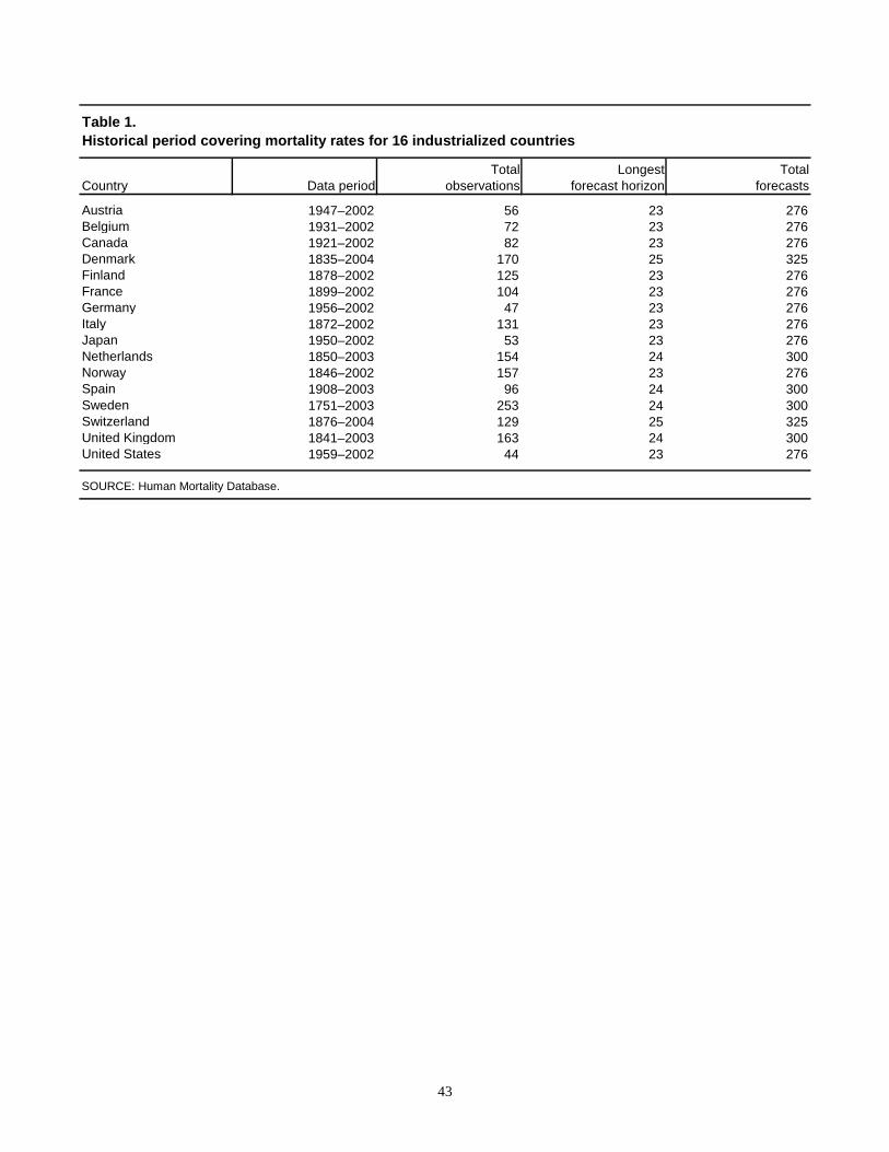
43
Country Data periodTotal
observationsLongest
forecast horizonTotal
forecasts
Austria 1947–2002 56 23 276Belgium 1931–2002 72 23 276Canada 1921–2002 82 23 276Denmark 1835–2004 170 25 325Finland 1878–2002 125 23 276France 1899–2002 104 23 276Germany 1956–2002 47 23 276Italy 1872–2002 131 23 276Japan 1950–2002 53 23 276Netherlands 1850–2003 154 24 300Norway 1846–2002 157 23 276Spain 1908–2003 96 24 300Sweden 1751–2003 253 24 300Switzerland 1876–2004 129 25 325United Kingdom 1841–2003 163 24 300United States 1959–2002 44 23 276
Table 1.Historical period covering mortality rates for 16 industrialized countries
SOURCE: Human Mortality Database.
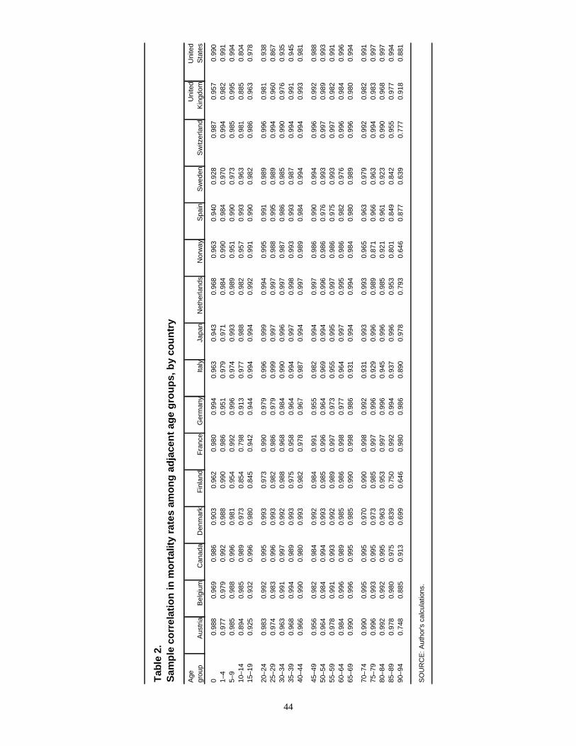
44
Age
grou
pA
ustr
iaB
elgi
umC
anad
aD
enm
ark
Fin
land
Fra
nce
Ger
man
yIta
lyJa
pan
Net
herla
nds
Nor
way
Spa
inS
wed
enS
witz
erla
ndU
nite
dK
ingd
omU
nite
dS
tate
s
00.
988
0.96
90.
986
0.90
30.
962
0.98
00.
994
0.96
30.
943
0.96
80.
963
0.94
00.
928
0.98
70.
957
0.99
01–
40.
977
0.97
90.
992
0.98
80.
990
0.98
60.
951
0.97
90.
971
0.98
40.
990
0.98
40.
970
0.99
40.
982
0.99
15–
90.
985
0.98
80.
996
0.98
10.
954
0.99
20.
996
0.97
40.
993
0.98
90.
951
0.99
00.
973
0.98
50.
995
0.99
410
–14
0.89
40.
985
0.98
90.
973
0.85
40.
798
0.91
30.
977
0.98
80.
982
0.95
70.
993
0.96
30.
981
0.88
50.
804
15–1
90.
925
0.93
20.
996
0.98
00.
845
0.94
20.
944
0.99
40.
994
0.99
20.
991
0.99
00.
982
0.98
60.
963
0.97
8
20–2
40.
983
0.99
20.
995
0.99
30.
973
0.99
00.
979
0.99
60.
999
0.99
40.
995
0.99
10.
989
0.99
60.
981
0.93
825
–29
0.97
40.
983
0.99
60.
993
0.98
20.
986
0.97
90.
999
0.99
70.
997
0.98
80.
995
0.98
90.
994
0.96
00.
867
30–3
40.
963
0.99
10.
997
0.99
20.
988
0.96
80.
984
0.99
00.
996
0.99
70.
987
0.98
60.
985
0.99
00.
976
0.93
535
–39
0.96
80.
994
0.98
90.
993
0.97
50.
958
0.96
40.
994
0.99
70.
998
0.99
30.
993
0.98
70.
994
0.99
10.
945
40–4
40.
966
0.99
00.
980
0.99
30.
982
0.97
80.
967
0.98
70.
994
0.99
70.
989
0.98
40.
994
0.99
40.
993
0.98
1
45–4
90.
956
0.98
20.
984
0.99
20.
984
0.99
10.
955
0.98
20.
994
0.99
70.
986
0.99
00.
994
0.99
60.
992
0.98
850
–54
0.96
40.
984
0.99
40.
993
0.98
50.
996
0.96
40.
969
0.99
40.
996
0.98
60.
976
0.99
30.
997
0.98
90.
993
55–5
90.
978
0.99
10.
993
0.99
20.
989
0.99
70.
973
0.95
50.
995
0.99
70.
986
0.97
50.
993
0.99
70.
982
0.99
160
–64
0.98
40.
996
0.98
90.
985
0.98
60.
998
0.97
70.
964
0.99
70.
995
0.98
60.
982
0.97
60.
996
0.98
40.
996
65–6
90.
990
0.99
60.
995
0.98
50.
990
0.99
80.
986
0.93
10.
994
0.99
40.
984
0.98
00.
989
0.99
60.
980
0.99
4
70–7
40.
990
0.99
50.
995
0.97
00.
990
0.99
80.
992
0.93
10.
993
0.99
30.
965
0.96
30.
979
0.99
20.
982
0.99
175
–79
0.99
60.
993
0.99
50.
973
0.98
50.
997
0.99
60.
929
0.99
60.
989
0.87
10.
966
0.96
30.
994
0.98
30.
997
80–8
40.
992
0.99
20.
995
0.96
30.
953
0.99
70.
996
0.94
50.
996
0.98
50.
921
0.96
10.
923
0.99
00.
968
0.99
785
–89
0.97
80.
980
0.97
50.
839
0.75
00.
992
0.99
40.
937
0.99
60.
953
0.80
10.
849
0.84
20.
955
0.97
70.
994
90–9
40.
748
0.88
50.
913
0.69
90.
646
0.98
00.
986
0.89
00.
978
0.79
30.
646
0.87
70.
639
0.77
70.
918
0.88
1
SO
UR
CE
: Aut
hor's
cal
cula
tions
.
Tab
le 2
.S
amp
le c
orr
elat
ion
in m
ort
alit
y ra
tes
amo
ng
ad
jace
nt
age
gro
up
s, b
y co
un
try
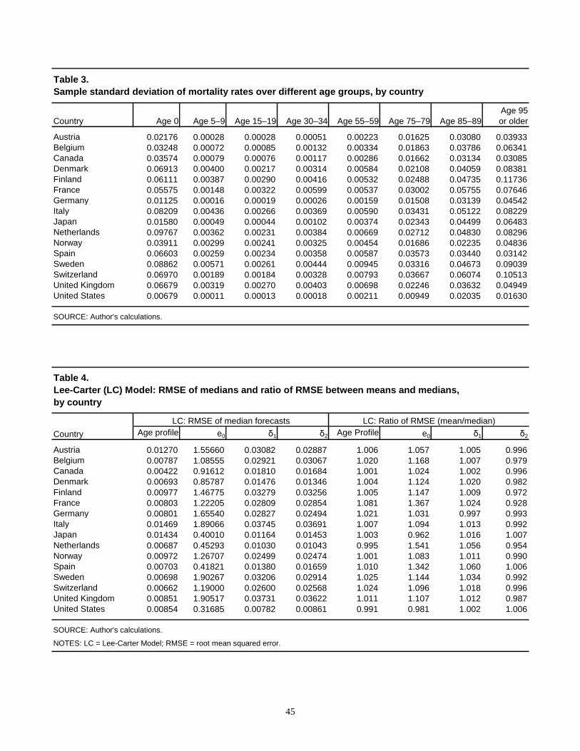
45
Country Age 0 Age 5–9 Age 15–19 Age 30–34 Age 55–59 Age 75–79 Age 85–89Age 95or older
Austria 0.02176 0.00028 0.00028 0.00051 0.00223 0.01625 0.03080 0.03933Belgium 0.03248 0.00072 0.00085 0.00132 0.00334 0.01863 0.03786 0.06341Canada 0.03574 0.00079 0.00076 0.00117 0.00286 0.01662 0.03134 0.03085Denmark 0.06913 0.00400 0.00217 0.00314 0.00584 0.02108 0.04059 0.08381Finland 0.06111 0.00387 0.00290 0.00416 0.00532 0.02488 0.04735 0.11736France 0.05575 0.00148 0.00322 0.00599 0.00537 0.03002 0.05755 0.07646Germany 0.01125 0.00016 0.00019 0.00026 0.00159 0.01508 0.03139 0.04542Italy 0.08209 0.00436 0.00266 0.00369 0.00590 0.03431 0.05122 0.08229Japan 0.01580 0.00049 0.00044 0.00102 0.00374 0.02343 0.04499 0.06483Netherlands 0.09767 0.00362 0.00231 0.00384 0.00669 0.02712 0.04830 0.08296Norway 0.03911 0.00299 0.00241 0.00325 0.00454 0.01686 0.02235 0.04836Spain 0.06603 0.00259 0.00234 0.00358 0.00587 0.03573 0.03440 0.03142Sweden 0.08862 0.00571 0.00261 0.00444 0.00945 0.03316 0.04673 0.09039Switzerland 0.06970 0.00189 0.00184 0.00328 0.00793 0.03667 0.06074 0.10513United Kingdom 0.06679 0.00319 0.00270 0.00403 0.00698 0.02246 0.03632 0.04949United States 0.00679 0.00011 0.00013 0.00018 0.00211 0.00949 0.02035 0.01630
SOURCE: Author's calculations.
Table 3.Sample standard deviation of mortality rates over different age groups, by country
Age profile e0 δ1 δ2 Age Profile e0 δ1 δ2
Austria 0.01270 1.55660 0.03082 0.02887 1.006 1.057 1.005 0.996Belgium 0.00787 1.08555 0.02921 0.03067 1.020 1.168 1.007 0.979Canada 0.00422 0.91612 0.01810 0.01684 1.001 1.024 1.002 0.996Denmark 0.00693 0.85787 0.01476 0.01346 1.004 1.124 1.020 0.982Finland 0.00977 1.46775 0.03279 0.03256 1.005 1.147 1.009 0.972France 0.00803 1.22205 0.02809 0.02854 1.081 1.367 1.024 0.928Germany 0.00801 1.65540 0.02827 0.02494 1.021 1.031 0.997 0.993Italy 0.01469 1.89066 0.03745 0.03691 1.007 1.094 1.013 0.992Japan 0.01434 0.40010 0.01164 0.01453 1.003 0.962 1.016 1.007Netherlands 0.00687 0.45293 0.01030 0.01043 0.995 1.541 1.056 0.954Norway 0.00972 1.26707 0.02499 0.02474 1.001 1.083 1.011 0.990Spain 0.00703 0.41821 0.01380 0.01659 1.010 1.342 1.060 1.006Sweden 0.00698 1.90267 0.03206 0.02914 1.025 1.144 1.034 0.992Switzerland 0.00662 1.19000 0.02600 0.02568 1.024 1.096 1.018 0.996United Kingdom 0.00851 1.90517 0.03731 0.03622 1.011 1.107 1.012 0.987United States 0.00854 0.31685 0.00782 0.00861 0.991 0.981 1.002 1.006
Table 4.Lee-Carter (LC) Model: RMSE of medians and ratio of RMSE between means and medians,by country
NOTES: LC = Lee-Carter Model; RMSE = root mean squared error.
SOURCE: Author's calculations.
Country
LC: RMSE of median forecasts LC: Ratio of RMSE (mean/median)
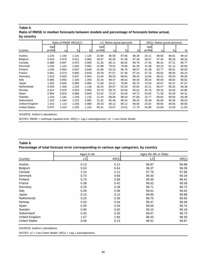
46
Age profile e0 δ1 δ2
Age profile e0 δ1 δ2
Age profile e0 δ1 δ2
Austria 1.224 1.194 1.141 1.125 22.89 96.59 97.85 98.28 20.11 98.60 99.81 99.43Belgium 0.918 0.979 0.911 0.865 49.87 95.39 97.49 97.49 48.67 97.40 98.26 98.26Canada 0.988 0.997 0.970 0.956 31.26 96.11 96.52 96.75 27.45 96.32 97.21 96.77Denmark 1.045 1.124 1.020 0.965 41.88 79.01 79.96 81.49 41.38 83.15 81.12 80.90Finland 1.045 0.954 0.947 0.848 41.88 93.24 96.76 98.07 41.38 93.77 98.81 98.83France 0.901 0.574 0.893 0.818 33.29 97.07 97.46 97.44 37.10 98.62 98.84 95.23Germany 1.013 0.933 0.937 0.944 15.40 98.03 98.64 98.25 15.06 98.41 99.03 99.05Italy 0.985 0.992 1.020 1.005 32.26 98.47 98.63 98.44 36.54 99.05 98.82 98.82Japan 1.002 0.845 0.985 0.969 71.89 20.47 78.85 85.70 70.50 29.67 83.37 87.07Netherlands 0.943 1.450 1.234 1.136 46.25 89.57 92.00 92.82 42.21 95.47 95.92 96.38Norway 0.914 0.978 0.924 0.900 33.79 89.76 93.63 95.51 33.76 90.33 93.62 94.86Spain 0.964 0.923 0.888 0.849 51.62 72.22 92.69 94.72 53.05 71.30 93.35 94.31Sweden 1.154 1.181 1.159 1.132 11.44 98.56 98.04 97.66 10.77 99.65 99.65 99.48Switzerland 1.102 1.044 1.023 0.982 31.32 95.46 98.04 98.20 30.38 96.83 98.36 98.53United Kingdom 1.023 1.114 1.035 0.989 29.33 99.12 99.12 98.94 25.92 99.65 99.65 99.65United States 0.970 1.413 1.235 1.191 50.41 33.07 19.01 17.79 54.86 24.64 13.05 11.82
SOURCE: Author's calculations.
NOTES: RMSE = rootmean squared error; AR(1) = Lag 1 autoregression; LC = Lee-Carter Model.
Table 5.Ratio of RMSE in median forecasts between models and percentage of forecasts below actual,by country
Country
Ratio of RMSE AR(1)/LC LC: Below actual (percent) AR(1): Below actual (percent)
LC AR(1) LC AR(1)
Austria 0.13 0.12 99.87 99.88Belgium 0.63 0.64 99.37 99.36Canada 2.24 2.12 97.76 97.88Denmark 0.70 0.66 99.30 99.34Finland 0.70 0.58 99.30 99.42France 0.38 0.42 99.62 99.58Germany 0.29 0.28 99.71 99.72Italy 0.39 0.38 99.61 99.62Japan 0.15 0.12 99.85 99.88Netherlands 0.25 0.35 99.75 99.65Norway 0.53 0.54 99.47 99.46Spain 0.35 0.26 99.65 99.74Sweden 0.90 0.82 99.10 99.18Switzerland 0.33 0.30 99.67 99.70United Kingdom 1.57 1.65 98.43 98.35United States 0.09 0.13 99.91 99.87
NOTES: LC = Lee-Carter Model; AR(1) = Lag 1 autoregression.
Table 6.Percentage of total forecast error corresponding to various age categories, by country
SOURCE: Author's calculations.
Country
Ages 0–64 Ages 65–95 or Older

47
Ages 0–19 Ages 20–64Ages 65–95
or older LC AR(1) LC AR(1) LC AR(1)
Austria 1.131 1.195 1.224 49.62 41.63 20.36 20.65 7.05 4.04Belgium 0.916 0.926 0.918 67.82 64.29 68.22 66.29 13.45 14.86Canada 1.166 0.951 0.989 52.79 50.86 39.59 39.17 37.03 37.47Denmark 0.883 1.038 1.045 36.77 31.71 33.17 29.38 24.87 21.92Finland 0.968 0.949 1.045 62.47 55.50 50.01 52.48 21.47 18.23France 0.624 1.019 0.901 31.56 44.02 54.50 56.21 7.25 7.60Germany 1.093 0.989 1.013 23.09 19.42 15.46 17.43 9.84 8.91Italy 0.930 1.001 0.986 52.51 62.96 43.17 47.96 3.76 2.99Japan 0.893 0.935 1.002 96.34 95.64 96.28 94.31 23.07 21.91Netherlands 0.989 1.130 0.942 38.87 36.90 58.71 54.69 35.51 29.96Norway 0.916 0.923 0.914 31.99 33.28 48.26 47.36 16.48 16.62Spain 0.720 1.039 0.964 68.86 68.63 71.87 74.11 13.29 14.84Sweden 0.929 1.152 1.154 18.29 19.60 8.14 7.54 10.79 8.60Switzerland 1.055 1.054 1.102 37.51 39.30 42.81 44.39 12.12 6.00United Kingdom 0.995 1.060 1.023 19.85 15.40 52.39 48.32 6.45 4.64United States 1.515 0.983 0.969 28.35 36.11 42.40 43.60 76.47 82.75
Country
Table 7.Ratio of RMSE in median forecasts between models and percentage of forecasts below actual,by country and broad age-categories
SOURCE: Author's calculations.
NOTES: RMSE = root mean squared error; AR(1) = Lag 1 autoregression; LC = Lee-Carter Model.
Ratio of RMSE AR(1)/LC Ages 0–19 Ages 20–64 Ages 65–95 or older
1–5 6–10 11–1516 ormore 1–5 6–10 11–15
16 ormore 1–5 6–10 11–15
16 ormore
Austria 1.015 1.160 1.213 1.249 36.04 22.50 19.01 17.35 32.90 20.87 16.97 13.60Belgium 0.930 0.953 0.973 0.874 49.92 51.35 51.15 48.12 45.98 49.55 50.54 48.64Canada 0.883 0.874 0.953 1.049 38.74 41.61 46.97 40.83 37.84 40.27 45.58 41.68Denmark 1.026 1.030 0.995 1.066 42.69 38.49 32.35 21.39 39.69 35.89 28.51 16.57Finland 1.011 0.952 0.955 1.125 40.89 40.62 44.74 46.05 34.87 40.26 45.03 45.03France 0.962 0.953 0.918 0.878 40.35 30.76 30.72 32.05 39.22 39.70 35.96 34.87Germany 0.996 1.004 1.000 1.019 28.56 22.03 12.37 4.93 28.42 23.76 13.97 1.97Italy 1.019 1.003 0.988 0.981 30.70 28.21 36.82 32.91 28.30 31.83 41.83 41.33Japan 0.996 1.033 1.023 0.995 68.01 72.06 74.11 72.83 63.03 70.47 74.26 72.83Netherlands 0.972 0.915 0.948 0.940 46.13 44.90 47.38 46.44 38.24 41.38 44.61 43.55Norway 0.932 0.954 0.905 0.874 43.42 36.34 30.18 28.45 41.93 37.17 29.41 29.25Spain 0.959 0.978 0.954 0.965 50.42 47.47 51.81 54.50 47.68 51.39 55.12 55.81Sweden 1.080 1.076 1.133 1.186 27.30 13.88 6.14 4.22 21.02 12.46 6.75 6.36Switzerland 1.056 1.077 1.079 1.115 38.76 30.11 29.34 29.19 34.45 29.13 28.73 29.81United Kingdom 0.968 1.010 1.026 1.027 36.26 31.89 27.75 24.94 30.11 29.22 25.87 21.79United States 0.975 0.961 0.962 0.972 51.02 50.57 50.56 49.84 54.09 55.28 57.03 53.74
SOURCE: Author's calculations.
NOTES: RMSE = root mean squared error; AR(1) = Lag 1 autoregression; LC = Lee-Carter Model.
Table 8.Ratio of RMSE in median forecasts of the age profile and percentage of forecasts below actual,by country and forecast horizon
Country
Ratio of RMSE AR(1)/LC LC: Below actual (percent) AR(1): Below actual (percent)
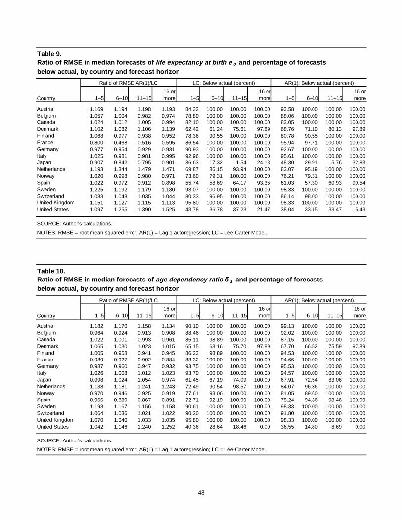
48
1–5 6–10 11–1516 ormore 1–5 6–10 11–15
16 ormore 1–5 6–10 11–15
16 ormore
Austria 1.169 1.194 1.198 1.193 84.32 100.00 100.00 100.00 93.58 100.00 100.00 100.00Belgium 1.057 1.004 0.982 0.974 78.80 100.00 100.00 100.00 88.06 100.00 100.00 100.00Canada 1.024 1.012 1.005 0.994 82.10 100.00 100.00 100.00 83.05 100.00 100.00 100.00Denmark 1.102 1.082 1.106 1.139 62.42 61.24 75.61 97.89 68.76 71.10 80.13 97.89Finland 1.068 0.977 0.938 0.952 78.36 90.55 100.00 100.00 80.78 90.55 100.00 100.00France 0.800 0.468 0.516 0.595 86.54 100.00 100.00 100.00 95.94 97.71 100.00 100.00Germany 0.977 0.954 0.929 0.931 90.93 100.00 100.00 100.00 92.67 100.00 100.00 100.00Italy 1.025 0.981 0.981 0.995 92.96 100.00 100.00 100.00 95.61 100.00 100.00 100.00Japan 0.907 0.842 0.795 0.901 36.63 17.32 1.54 24.18 48.30 29.91 5.76 32.83Netherlands 1.193 1.344 1.479 1.471 69.87 86.15 93.94 100.00 83.07 95.19 100.00 100.00Norway 1.020 0.998 0.980 0.971 73.60 79.31 100.00 100.00 76.21 79.31 100.00 100.00Spain 1.022 0.972 0.912 0.898 55.74 58.69 64.17 93.36 61.03 57.30 60.93 90.54Sweden 1.225 1.192 1.179 1.180 93.07 100.00 100.00 100.00 98.33 100.00 100.00 100.00Switzerland 1.083 1.048 1.035 1.044 80.33 96.95 100.00 100.00 86.14 98.00 100.00 100.00United Kingdom 1.151 1.127 1.115 1.113 95.80 100.00 100.00 100.00 98.33 100.00 100.00 100.00United States 1.097 1.255 1.390 1.525 43.78 36.78 37.23 21.47 38.04 33.15 33.47 5.43
SOURCE: Author's calculations.
NOTES: RMSE = root mean squared error; AR(1) = Lag 1 autoregression; LC = Lee-Carter Model.
Table 9.Ratio of RMSE in median forecasts of life expectancy at birth e 0 and percentage of forecastsbelow actual, by country and forecast horizon
Country
Ratio of RMSE AR(1)/LC LC: Below actual (percent) AR(1): Below actual (percent)
1–5 6–10 11–1516 ormore 1–5 6–10 11–15
16 ormore 1–5 6–10 11–15
16 ormore
Austria 1.182 1.170 1.158 1.134 90.10 100.00 100.00 100.00 99.13 100.00 100.00 100.00Belgium 0.964 0.924 0.913 0.908 88.46 100.00 100.00 100.00 92.02 100.00 100.00 100.00Canada 1.022 1.001 0.993 0.961 85.11 98.89 100.00 100.00 87.15 100.00 100.00 100.00Denmark 1.065 1.030 1.023 1.015 65.15 63.16 75.70 97.89 67.70 66.52 75.59 97.89Finland 1.005 0.958 0.941 0.945 86.23 98.89 100.00 100.00 94.53 100.00 100.00 100.00France 0.989 0.927 0.902 0.884 88.32 100.00 100.00 100.00 94.66 100.00 100.00 100.00Germany 0.987 0.960 0.947 0.932 93.75 100.00 100.00 100.00 95.53 100.00 100.00 100.00Italy 1.026 1.008 1.012 1.023 93.70 100.00 100.00 100.00 94.57 100.00 100.00 100.00Japan 0.998 1.024 1.054 0.974 61.45 67.19 74.09 100.00 67.91 72.54 83.06 100.00Netherlands 1.138 1.181 1.241 1.243 72.49 90.54 98.57 100.00 84.07 96.36 100.00 100.00Norway 0.970 0.946 0.925 0.919 77.61 93.06 100.00 100.00 81.05 89.60 100.00 100.00Spain 0.966 0.880 0.867 0.891 72.71 92.19 100.00 100.00 75.24 94.36 98.46 100.00Sweden 1.198 1.167 1.156 1.158 90.61 100.00 100.00 100.00 98.33 100.00 100.00 100.00Switzerland 1.064 1.036 1.021 1.022 90.20 100.00 100.00 100.00 91.80 100.00 100.00 100.00United Kingdom 1.070 1.040 1.033 1.035 95.80 100.00 100.00 100.00 98.33 100.00 100.00 100.00United States 1.042 1.146 1.240 1.252 40.36 28.64 18.46 0.00 36.55 14.80 8.69 0.00
SOURCE: Author's calculations.
NOTES: RMSE = root mean squared error; AR(1) = Lag 1 autoregression; LC = Lee-Carter Model.
Table 10.Ratio of RMSE in median forecasts of age dependency ratio δ 1 and percentage of forecastsbelow actual, by country and forecast horizon
Country
Ratio of RMSE AR(1)/LC LC: Below actual (percent) AR(1): Below actual (percent)
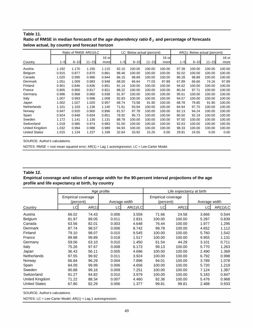
49
1–5 6–10 11–1516 ormore 1–5 6–10 11–15
16 ormore 1–5 6–10 11–15
16 ormore
Austria 1.192 1.170 1.150 1.115 92.10 100.00 100.00 100.00 97.39 100.00 100.00 100.00Belgium 0.915 0.877 0.870 0.861 88.46 100.00 100.00 100.00 92.02 100.00 100.00 100.00Canada 1.020 0.995 0.986 0.944 86.15 98.89 100.00 100.00 86.28 98.89 100.00 100.00Denmark 1.051 1.009 0.983 0.948 68.00 66.64 77.03 97.89 67.89 66.66 74.16 97.89Finland 0.901 0.846 0.836 0.851 91.14 100.00 100.00 100.00 94.62 100.00 100.00 100.00France 0.805 0.800 0.817 0.821 88.22 100.00 100.00 100.00 80.34 97.71 100.00 100.00Germany 0.996 0.968 0.960 0.938 91.97 100.00 100.00 100.00 95.61 100.00 100.00 100.00Italy 1.007 0.993 0.998 1.008 92.83 100.00 100.00 100.00 94.57 100.00 100.00 100.00Japan 1.002 1.027 1.020 0.957 68.74 73.58 91.90 100.00 68.78 79.85 91.90 100.00Netherlands 1.101 1.103 1.136 1.140 71.61 93.94 100.00 100.00 84.94 97.70 100.00 100.00Norway 0.947 0.920 0.900 0.896 81.57 97.78 100.00 100.00 82.13 94.24 100.00 100.00Spain 0.924 0.848 0.834 0.851 78.92 95.73 100.00 100.00 80.50 92.19 100.00 100.00Sweden 1.172 1.141 1.130 1.131 88.78 100.00 100.00 100.00 97.50 100.00 100.00 100.00Switzerland 1.018 0.985 0.974 0.983 91.00 100.00 100.00 100.00 92.63 100.00 100.00 100.00United Kingdom 1.032 0.994 0.988 0.989 94.93 100.00 100.00 100.00 98.33 100.00 100.00 100.00United States 1.015 1.134 1.237 1.199 32.64 33.92 15.25 0.00 29.81 24.55 0.00 0.00
SOURCE: Author's calculations.
NOTES: RMSE = root mean squared error; AR(1) = Lag 1 autoregression; LC = Lee-Carter Model.
Table 11.Ratio of RMSE in median forecasts of the age dependency ratio δ 2 and percentage of forecastsbelow actual, by country and forecast horizon
Country
Ratio of RMSE AR(1)/LC LC: Below actual (percent) AR(1): Below actual (percent)
LC AR(1) LC AR(1)/LC LC AR(1) LC AR(1)/LC
Austria 66.02 74.43 0.006 3.559 71.66 24.58 3.666 0.544Belgium 81.97 89.05 0.011 2.831 100.00 100.00 5.287 0.839Canada 63.56 82.01 0.003 4.648 76.44 100.00 1.977 1.295Denmark 87.74 98.57 0.006 8.742 99.78 100.00 4.652 1.112Finland 79.10 98.07 0.010 9.545 100.00 100.00 5.760 1.542France 99.88 99.89 0.018 1.517 100.00 100.00 9.955 1.131Germany 59.06 63.10 0.010 1.450 61.54 44.29 3.101 0.711Italy 75.26 97.67 0.008 6.173 99.13 100.00 5.770 1.263Japan 36.43 56.11 0.005 4.696 100.00 100.00 2.490 1.369Netherlands 97.55 99.92 0.011 3.924 100.00 100.00 6.792 0.998Norway 66.84 96.29 0.004 7.896 94.01 100.00 3.789 1.078Spain 84.09 99.99 0.006 4.656 100.00 100.00 5.720 1.219Sweden 90.88 99.16 0.009 7.251 100.00 100.00 7.124 1.387Switzerland 91.27 94.82 0.010 3.979 100.00 100.00 5.183 0.847United Kingdom 71.22 88.34 0.007 4.460 92.36 100.00 5.476 0.968United States 67.80 82.29 0.006 1.377 99.81 99.81 2.488 0.933
NOTES: LC = Lee-Carter Model; AR(1) = Lag 1 autoregression.
Country
SOURCE: Author's calculations.
Table 12.Empirical coverage and ratios of average width for the 90-percent interval projections of the ageprofile and life expectancy at birth, by country
Empirical coverage(percent) Average width
Empirical coverage(percent) Average width
Age profile Life expectancy at birth
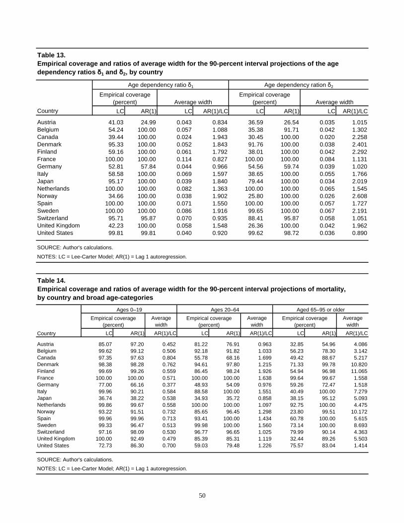
50
LC AR(1) LC AR(1)/LC LC AR(1) LC AR(1)/LC
Austria 41.03 24.99 0.043 0.834 36.59 26.54 0.035 1.015Belgium 54.24 100.00 0.057 1.088 35.38 91.71 0.042 1.302Canada 39.44 100.00 0.024 1.943 30.45 100.00 0.020 2.258Denmark 95.33 100.00 0.052 1.843 91.76 100.00 0.038 2.401Finland 59.16 100.00 0.061 1.792 38.01 100.00 0.042 2.292France 100.00 100.00 0.114 0.827 100.00 100.00 0.084 1.131Germany 52.81 57.84 0.044 0.966 54.56 59.74 0.039 1.020Italy 58.58 100.00 0.069 1.597 38.65 100.00 0.055 1.766Japan 95.17 100.00 0.039 1.840 79.44 100.00 0.034 2.019Netherlands 100.00 100.00 0.082 1.363 100.00 100.00 0.065 1.545Norway 34.66 100.00 0.038 1.902 25.80 100.00 0.026 2.608Spain 100.00 100.00 0.071 1.550 100.00 100.00 0.057 1.727Sweden 100.00 100.00 0.086 1.916 99.65 100.00 0.067 2.191Switzerland 95.71 95.87 0.070 0.935 88.41 95.87 0.058 1.051United Kingdom 42.23 100.00 0.058 1.548 26.36 100.00 0.042 1.962United States 99.81 99.81 0.040 0.920 99.62 98.72 0.036 0.890
NOTES: LC = Lee-Carter Model; AR(1) = Lag 1 autoregression.
Country
SOURCE: Author's calculations.
Table 13.Empirical coverage and ratios of average width for the 90-percent interval projections of the agedependency ratios δ1 and δ2, by country
Empirical coverage(percent) Average width
Empirical coverage(percent) Average width
Age dependency ratio δ1 Age dependency ration δ2
Average width
Average width
Average width
LC AR(1) AR(1)/LC LC AR(1) AR(1)/LC LC AR(1) AR(1)/LC
Austria 85.07 97.20 0.452 81.22 76.91 0.963 32.85 54.96 4.086Belgium 99.62 99.12 0.506 92.18 91.82 1.033 56.23 78.30 3.142Canada 97.35 97.63 0.804 55.78 68.16 1.699 49.42 88.67 5.217Denmark 98.38 98.28 0.762 94.61 97.80 1.215 71.33 99.78 10.820Finland 99.69 99.26 0.559 86.45 98.24 1.926 54.94 96.98 11.065France 100.00 100.00 0.571 100.00 100.00 1.638 99.64 99.67 1.558Germany 77.00 66.16 0.377 48.93 54.09 0.976 59.26 72.47 1.518Italy 99.96 90.21 0.584 88.58 100.00 1.551 40.49 100.00 7.279Japan 36.74 38.22 0.538 34.93 35.72 0.858 38.15 95.12 5.093Netherlands 99.86 99.67 0.558 100.00 100.00 1.097 92.75 100.00 4.475Norway 93.22 91.51 0.732 85.65 96.45 1.298 23.80 99.51 10.172Spain 99.96 99.96 0.713 93.41 100.00 1.434 60.78 100.00 5.615Sweden 99.33 96.47 0.513 99.98 100.00 1.560 73.14 100.00 8.693Switzerland 97.16 98.09 0.530 96.77 96.65 1.025 79.99 90.14 4.363United Kingdom 100.00 92.49 0.479 85.39 85.31 1.119 32.44 89.26 5.503United States 72.73 86.30 0.700 59.03 79.48 1.226 75.57 83.04 1.414
Table 14.Empirical coverage and ratios of average width for the 90-percent interval projections of mortality,by country and broad age-categories
SOURCE: Author's calculations.
NOTES: LC = Lee-Carter Model; AR(1) = Lag 1 autoregression.
Empirical coverage(percent)
Ages 0–19 Ages 20–64 Aged 65–95 or older
Country
Empirical coverage(percent)
Empirical coverage(percent)
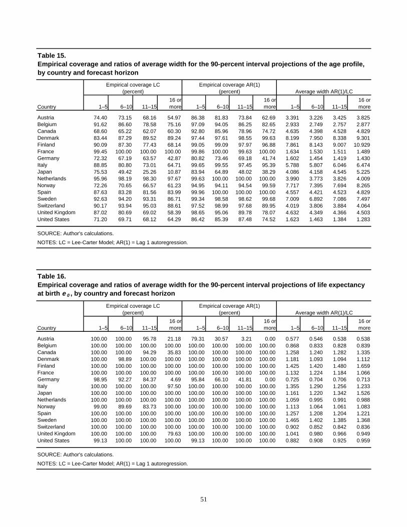
51
1–5 6–10 11–1516 ormore 1–5 6–10 11–15
16 ormore 1–5 6–10 11–15
16 ormore
Austria 74.40 73.15 68.16 54.97 86.38 81.83 73.84 62.69 3.391 3.226 3.425 3.825Belgium 91.62 86.60 78.58 75.16 97.09 94.05 86.25 82.65 2.933 2.749 2.757 2.877Canada 68.60 65.22 62.07 60.30 92.80 85.96 78.96 74.72 4.635 4.398 4.528 4.829Denmark 83.44 87.29 89.52 89.24 97.44 97.61 98.55 99.63 8.199 7.950 8.338 9.301Finland 90.09 87.30 77.43 68.14 99.05 99.09 97.97 96.88 7.861 8.143 9.007 10.929France 99.45 100.00 100.00 100.00 99.86 100.00 99.63 100.00 1.634 1.530 1.511 1.489Germany 72.32 67.19 63.57 42.87 80.82 73.46 69.18 41.74 1.602 1.454 1.419 1.430Italy 88.85 80.80 73.01 64.71 99.65 99.55 97.45 95.39 5.788 5.807 6.046 6.474Japan 75.53 49.42 25.26 10.87 83.94 64.89 48.02 38.29 4.086 4.158 4.545 5.225Netherlands 95.96 98.19 98.30 97.67 99.63 100.00 100.00 100.00 3.990 3.773 3.826 4.009Norway 72.26 70.65 66.57 61.23 94.95 94.11 94.54 99.59 7.717 7.395 7.694 8.265Spain 87.63 83.28 81.56 83.99 99.96 100.00 100.00 100.00 4.557 4.421 4.523 4.829Sweden 92.63 94.20 93.31 86.71 99.34 98.58 98.62 99.68 7.009 6.892 7.086 7.497Switzerland 90.17 93.94 95.03 88.61 97.52 98.99 97.68 89.95 4.019 3.806 3.884 4.064United Kingdom 87.02 80.69 69.02 58.39 98.65 95.06 89.78 78.07 4.632 4.349 4.366 4.503United States 71.20 69.71 68.12 64.29 86.42 85.39 87.48 74.52 1.623 1.463 1.384 1.283
SOURCE: Author's calculations.
NOTES: LC = Lee-Carter Model; AR(1) = Lag 1 autoregression.
Table 15.Empirical coverage and ratios of average width for the 90-percent interval projections of the age profile,by country and forecast horizon
Country
Empirical coverage LC(percent)
Empirical coverage AR(1)(percent) Average width AR(1)/LC
1–5 6–10 11–1516 ormore 1–5 6–10 11–15
16 ormore 1–5 6–10 11–15
16 ormore
Austria 100.00 100.00 95.78 21.18 79.31 30.57 3.21 0.00 0.577 0.546 0.538 0.538Belgium 100.00 100.00 100.00 100.00 100.00 100.00 100.00 100.00 0.868 0.833 0.828 0.839Canada 100.00 100.00 94.29 35.83 100.00 100.00 100.00 100.00 1.258 1.240 1.282 1.335Denmark 100.00 98.89 100.00 100.00 100.00 100.00 100.00 100.00 1.181 1.093 1.094 1.112Finland 100.00 100.00 100.00 100.00 100.00 100.00 100.00 100.00 1.425 1.420 1.480 1.659France 100.00 100.00 100.00 100.00 100.00 100.00 100.00 100.00 1.132 1.224 1.184 1.066Germany 98.95 92.27 84.37 4.69 95.84 66.10 41.81 0.00 0.725 0.704 0.706 0.713Italy 100.00 100.00 100.00 97.50 100.00 100.00 100.00 100.00 1.355 1.290 1.256 1.233Japan 100.00 100.00 100.00 100.00 100.00 100.00 100.00 100.00 1.161 1.220 1.342 1.526Netherlands 100.00 100.00 100.00 100.00 100.00 100.00 100.00 100.00 1.059 0.995 0.991 0.988Norway 99.00 89.69 83.73 100.00 100.00 100.00 100.00 100.00 1.113 1.064 1.061 1.083Spain 100.00 100.00 100.00 100.00 100.00 100.00 100.00 100.00 1.257 1.208 1.204 1.221Sweden 100.00 100.00 100.00 100.00 100.00 100.00 100.00 100.00 1.465 1.402 1.385 1.368Switzerland 100.00 100.00 100.00 100.00 100.00 100.00 100.00 100.00 0.902 0.852 0.842 0.836United Kingdom 100.00 100.00 100.00 79.63 100.00 100.00 100.00 100.00 1.041 0.980 0.966 0.949United States 99.13 100.00 100.00 100.00 99.13 100.00 100.00 100.00 0.882 0.908 0.925 0.959
SOURCE: Author's calculations.
NOTES: LC = Lee-Carter Model; AR(1) = Lag 1 autoregression.
Table 16.Empirical coverage and ratios of average width for the 90-percent interval projections of life expectancyat birth e 0 , by country and forecast horizon
Country
Empirical coverage LC(percent)
Empirical coverage AR(1)(percent) Average width AR(1)/LC
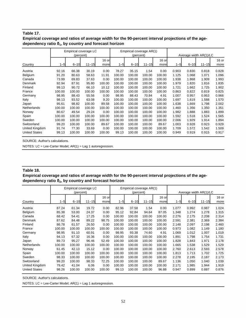
52
1–5 6–10 11–1516 ormore 1–5 6–10 11–15
16 ormore 1–5 6–10 11–15
16 ormore
Austria 92.16 66.38 30.19 0.00 78.27 35.15 1.54 0.00 0.903 0.830 0.818 0.828Belgium 91.20 80.63 58.63 11.91 100.00 100.00 100.00 100.00 1.125 1.068 1.071 1.096Canada 73.99 69.83 37.63 0.00 100.00 100.00 100.00 100.00 1.938 1.868 1.909 1.993Denmark 92.94 87.91 95.80 100.00 100.00 100.00 100.00 100.00 1.979 1.820 1.816 1.835Finland 99.13 90.72 66.10 10.12 100.00 100.00 100.00 100.00 1.721 1.662 1.725 1.902France 100.00 100.00 100.00 100.00 100.00 100.00 100.00 100.00 0.863 0.822 0.819 0.825Germany 98.95 88.43 55.56 0.00 98.95 88.43 70.84 4.91 1.007 0.957 0.953 0.966Italy 98.13 93.52 63.08 9.20 100.00 100.00 100.00 100.00 1.697 1.619 1.588 1.570Japan 95.61 98.82 100.00 89.58 100.00 100.00 100.00 100.00 1.638 1.669 1.798 2.002Netherlands 100.00 100.00 100.00 100.00 100.00 100.00 100.00 100.00 1.460 1.356 1.350 1.351Norway 80.67 49.54 29.24 0.00 100.00 100.00 100.00 100.00 1.982 1.888 1.883 1.899Spain 100.00 100.00 100.00 100.00 100.00 100.00 100.00 100.00 1.592 1.518 1.524 1.565Sweden 100.00 100.00 100.00 100.00 100.00 100.00 100.00 100.00 2.006 1.929 1.914 1.894Switzerland 99.20 100.00 100.00 89.67 100.00 100.00 100.00 89.67 1.003 0.928 0.923 0.929United Kingdom 91.74 77.30 33.69 0.00 100.00 100.00 100.00 100.00 1.709 1.572 1.542 1.509United States 99.13 100.00 100.00 100.00 99.13 100.00 100.00 100.00 0.949 0.919 0.915 0.917
SOURCE: Author's calculations.
NOTES: LC = Lee-Carter Model; AR(1) = Lag 1 autoregression.
Table 17.Empirical coverage and ratios of average width for the 90-percent interval projections of the age-dependency ratio δ1, by country and forecast horizon
Country
Empirical coverage LC(percent)
Empirical coverage AR(1)(percent) Average width AR(1)/LC
1–5 6–10 11–1516 ormore 1–5 6–10 11–15
16 ormore 1–5 6–10 11–15
16 ormore
Austria 87.24 61.34 19.72 0.00 82.96 37.58 1.54 0.00 1.077 0.992 0.987 1.024Belgium 85.38 53.00 24.37 0.00 95.12 92.84 94.64 87.05 1.348 1.274 1.278 1.315Canada 68.42 54.41 17.25 0.00 100.00 100.00 100.00 100.00 2.276 2.175 2.208 2.314Denmark 87.62 84.48 89.22 98.75 100.00 100.00 100.00 100.00 2.591 2.381 2.369 2.384Finland 86.78 61.57 26.50 0.00 100.00 100.00 100.00 100.00 2.148 2.097 2.198 2.460France 100.00 100.00 100.00 100.00 100.00 100.00 100.00 100.00 0.973 1.082 1.149 1.180Germany 98.95 91.10 60.91 0.00 98.95 93.38 74.60 4.91 1.069 1.012 1.007 1.019Italy 94.13 67.32 16.36 0.00 100.00 100.00 100.00 100.00 1.891 1.798 1.754 1.731Japan 89.73 95.27 96.46 52.49 100.00 100.00 100.00 100.00 1.828 1.843 1.971 2.178Netherlands 100.00 100.00 100.00 100.00 100.00 100.00 100.00 100.00 1.665 1.538 1.529 1.529Norway 61.45 42.13 15.12 0.00 100.00 100.00 100.00 100.00 2.760 2.613 2.593 2.578Spain 100.00 100.00 100.00 100.00 100.00 100.00 100.00 100.00 1.813 1.713 1.702 1.725Sweden 98.33 100.00 100.00 100.00 100.00 100.00 100.00 100.00 2.278 2.195 2.187 2.173Switzerland 99.20 100.00 98.33 72.25 100.00 100.00 100.00 89.67 1.136 1.050 1.040 1.039United Kingdom 79.42 41.04 6.06 0.00 100.00 100.00 100.00 100.00 2.171 1.985 1.944 1.919United States 98.26 100.00 100.00 100.00 99.13 100.00 100.00 96.88 0.947 0.899 0.887 0.876
SOURCE: Author's calculations.
NOTES: LC = Lee-Carter Model; AR(1) = Lag 1 autoregression.
Table 18.Empirical coverage and ratios of average width for the 90-percent interval projections of the age-dependency ratio δ2, by country and forecast horizon
Country
Empirical coverage LC(percent)
Empirical coverage AR(1)(percent) Average width AR(1)/LC
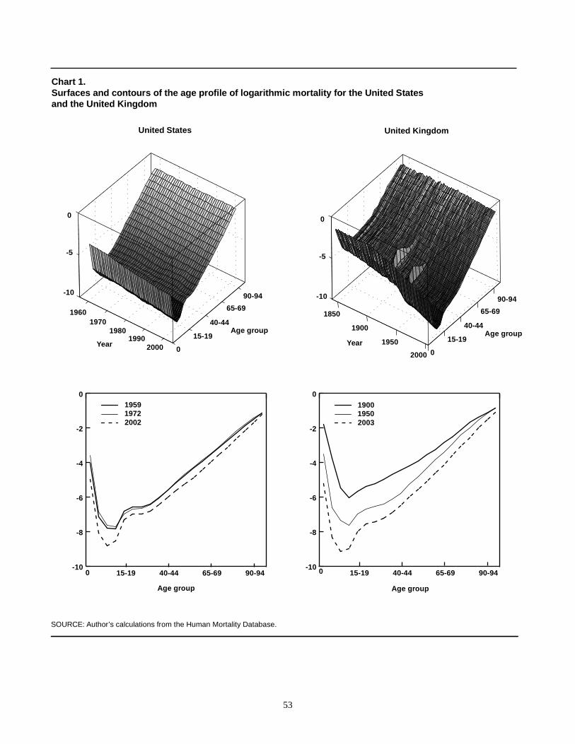
53
Chart 1.Surfaces and contours of the age profile of logarithmic mortality for the United Statesand the United Kingdom
SOURCE: Author’s calculations from the Human Mortality Database.
United States United Kingdom
-10
-8
-6
-4
-2
0
90-9465-6940-4415-19-10
-8
-6
-4
-2
0
90-9465-6940-4415-19
Age group Age group
0 0
195919722002
190019502003
-10
-5
0
-10
-5
0
19601970
19801990
2000
90-94
65-69
40-44
15-19
0
Age group
Year
90-94
65-69
40-44
15-19
0
Age group
1850
1900
1950
2000
Year
54
Chart 2.Mortality projections for ages 10–14 and ages 70–74 for the United States (1980–2002) andthe United Kingdom (1980–2003)
SOURCE: Author’s calculations.
NOTE: AR(1) = Lag 1 autoregression.
0.020
0.030
0.040
0.050
200019951990198519801975197019651960
Year
Year
United States United KingdomMortality projections for ages 10–14
0.0001
0.0002
0.0003
0.0004
0.0005
200019951990198519801975197019651960
Mortality projections for ages 70–74
ActualLee-CarterAR(1)
ActualLee-CarterAR(1)
0
0.001
0.002
0.003
0.004
200019801960194019201900
Year
0.02
0.04
0.06
0.08
0.10
200019801960194019201900
ActualLee-CarterAR(1)
ActualLee-CarterAR(1)
Year
55
Chart 3.Life expectancy at birth and old-age dependency ratios for the United States and the United Kingdom
SOURCE: Author’s calculations.
NOTE: AR(1) = Lag 1 autoregression.
0.0
0.2
0.4
0.6
0.8
1.0
200019951990198519801975197019651960
Year Year
Year Year
United States United KingdomLife expectancy at birth e0
68
70
72
74
76
78
80
20001995199019851980197519701965196035
40
45
50
55
60
65
70
75
80
200019801960194019201900
0.0
0.2
0.4
0.6
0.8
1.0
200019801960194019201900
Old-age dependency ratios
ActualLee-CarterAR(1)
ActualLee-CarterAR(1)
δ2 (actual population)δ2 (implied by mortality)δ1 (actual population)
δ1 (implied by mortality)
δ2 (actual population)δ2 (implied by mortality)δ1 (actual population)
δ1 (implied by mortality)
56
Chart 4.Projections of old-age dependency ratios for the United States (1980-2002) andthe United Kingdom (1980-2003)
SOURCE: Author’s calculations.
NOTE: AR(1) = Lag 1 autoregression.
0.70
0.75
0.80
0.85
0.90
0.95
200019951990198519801975197019651960
Year Year
Year Year
United States United KingdomOld-age dependency ratio δ1
0.24
0.26
0.28
0.30
0.32
0.34
0.36
0.38
0.40
0.42
2000199519901985198019751970196519600.10
0.15
0.20
0.25
0.30
0.35
0.40
1980 20001960194019201900
0.70
0.75
0.80
0.85
0.90
0.95
200019801960194019201900
Old-age dependency ratio δ2
ActualLee-CarterAR(1)
ActualLee-CarterAR(1)
ActualLee-CarterAR(1)
ActualLee-CarterAR(1)

57
References
Bell, W. 1997. Comparing and assessing time series methods for forecasting age-specific fertility and mortality rates. Journal of Official Statistics 13(3): 279-303.
Bell, W., and B. Monsell. 1991. Using principal components in time series modeling and forecasting of age-specific mortality rates. Paper presented at the 1991 Annual Meetings of the Population Association of America, Washington, DC.
Board of Trustees of the Federal Old-Age and Survivors Insurance and Disability Insurance Trust Funds. 2005. 2005 Annual Report. Washington, DC: U.S. Government Printing Office.
Congressional Budget Office. 2001. Uncertainty in Social Security's long-term finances: A stochastic analysis. Washington, DC: U.S. Government Printing Office.
Denton, F. T., C. H. Feaver, and B. G. Spencer. 2005. Time series analysis and stochastic forecasting: An econometric study of mortality and life expectancy. Journal of Population Economics 18: 203-227.
Girosi, F., and G. King. 2004. Demographic Forecasting. Unpublished book manuscript.
Lee, R. D. 2000. The Lee-Carter method for forecasting mortality, with various extensions and applications. North American Actuarial Journal 4(1): 80-91.
Lee, R. D., and L. R. Carter. 1992. Modeling and forecasting U.S. mortality. Journal of the American Statistical Association 87: 659-671.
Lee, R. D., and T. Miller. 2001. Evaluating the performance of the Lee-Carter method for forecasting mortality. Demography 38(4): 537-549.
Wilmoth, J. 1993. Computational methods for fitting and extrapolating the Lee-Carter model of mortality change. Technical Report, Department of Demography, University of California, Berkeley.
———. Methods protocol for the human mortality database. Technical Report. Available at www.mortality.org.

58
ORES Working Paper Series
Recent Working Papers Number Date Title and Author 111 July The Out-of-Sample Performance of Stochastic Methods in 2008 Forecasting Age-Specific Mortality Rates by Javier Meseguer 110 December Cohort-Specific Measures of Lifetime Social Security 2007 Taxes and Benefits by Dean R. Leimer 109 October Social Security as a Retirement Resource for Near-Retirees, 2007 by Race and Ethnicity, Nativity, Benefit Type, and Disability Status by Benjamin Bridges and Sharmila Choudhury 108 October Trends in Mortality Differentials and Life Expectancy for Male 2007 Social Security–Covered Workers, by Average Relative Earnings by Hilary Waldron 107 July New Evidence on Earnings and Benefit Claims Following Changes in 2006 the Retirement Earnings Test in 2000 by Jae G. Song and Joyce Manchester 106 May Social Security as a Retirement Resource for Near-Retirees 2005 by Benjamin Bridges and Sharmila Choudbury 105 May Heterogeneity in Health and Mortality Risk Among Early Retiree Men 2004 by Hilary Waldron 104 April Using Predisability Earnings as an Instrument for Disability 2004 Determination Outcomes by Jae G. Song 103 March Young Widow(er)s, Social Security, and Marriage 2004 by Michael J. Brien, Stacy Dickert-Conlin, and David A. Weaver 102 February Historical Redistribution Under the Social Security Old-Age and 2004 Survivors Insurance and Disability Insurance Programs by Dean R. Leimer 101 April Historical Redistribution Under the Social Security Old-Age and 2003 Survivors Insurance Program by Dean R. Leimer
99 December Mortality Differentials by Race 2002 by Hilary Waldron 98 August Social Security Disability Programs: Assessing 2002 the Variation in Allowance Rates by Alexander Strand

59
Recent Working Papers—Continued Number Date Title and Author 97 July Do Early Retirees Die Early?
2002 Evidence from Three Independent Data Sets by Hilary Waldron
96 June Social Security Benefit Reporting in the Survey of Income and Program
2002 Participation and in Social Security Administrative Records by Janice A. Olson 95 April Racial and Ethnic Differences in Wealth Holdings 2002 and Portfolio Choices by Sharmila Choudhury 94 September Income Growth and Future Poverty Rates of the Aged 2001 by Seyda G. Wentworth and David Pattison 93 August Links Between Early Retirement and Mortality 2001 by Hilary Waldron 92 June The Widow(er)’s Limit Provision of Social Security 2001 by David A. Weaver 91 June Methods in Modeling Income in the Near Term (MINT I) 2001 by Barbara A. Butrica, Howard M. Iams, James H. Moore, and
Mikki D. Waid 90 January Counting the Disabled: Using Survey Self-Reports to Estimate Medical 2001 Eligibility for Social Security’s Disability Programs by Debra Dwyer, Jianting Hu, Denton R. Vaughan, and
Bernard Wixon 89 January Widows Waiting to Wed? (Re)Marriage and Economic Incentives 2001 in Social Security Widow Benefits by Michael J. Brien, Stacy Dickert-Conlin, and David A. Weaver 88 January Analysis of Social Security Proposals Intended to Help Women: 2001 Preliminary Results by Sharmila Choudhury, Michael V. Leonesio, Kelvin R. Utendorf,
Linda Del Bene, and Robert V. Gesumaria 87 January Reducing Poverty Among Elderly Women 2001 by Michael A. Anzick and David A. Weaver 86 August Early Retirees Under Social Security: Health Status and Economic 2000 Resources by Michael V. Leonesio, Denton R. Vaughan, and Bernard Wixon 85 September Who is “62 Enough”: Identifying Eligibles for Social Security Early 1999 Retirement in the Health and Retirement Study by Janice A. Olson

60
Recent Working Papers—Continued Number Date Title and Author 84 August Linkages with Data from Social Security Administrative Records in 1999 the Health and Retirement Study by Janice A. Olson 83 July Characteristics of Individuals with Integrated Pensions 1999 by Keith A. Bender 82 April Recent Changes in Earnings Distributions in the United States: Age 1999 and Cohort Effects by Kelvin R. Utendorf
81 April Lifetime Redistribution Under the Social Security Program: A Literature 1999 Synopsis
by Dean R. Leimer 80 January The Accuracy of Survey-Reported Marital Status: Evidence from Survey 1999 Records Matched to Social Security Records by David A. Weaver 79 November Retirement Income Security in the United Kingdom 1998 by Lillian Liu 78 November Projecting Immigrant Earnings: The Significance of Country of Origin 1998 by Harriet Orcutt Duleep and Mark C. Regets 77 July Historical Redistribution Under the Social Security Disability Insurance 1998 Program by Dean R. Leimer 76 July Recent Changes in Earnings Distributions in the United States 1998 by Kelvin R. Utendorf 75 July Pension Integration and Social Security Reform 1998 by Chuck Slusher 74 January The Retirement Prospects of the Baby Boom Generation 1998 by Daniel B. Radner 73 December The Economic Well-Being of Social Security Beneficiaries, with 1997 an Emphasis on Divorced Beneficiaries by David A. Weaver 72 August A Structural Model of Social Security's Disability Determination Process 1997 by Jianting Hu, Kajal Lahiri, Denton R. Vaughan, and
Bernard Wixon 71 April Life-Cycle Aspects of Poverty Among Older Women 1997 by Sharmila Choudhury and Michael V. Leonesio 70 November Family Unit Incomes of the Elderly and Children, 1994 1996 by Daniel B. Radner

61
Recent Working Papers—Continued Number Date Title and Author 69 June Social Security and Immigrant Earnings 1996 by Harriet Orcutt Duleep and Mark C. Regets 68 October Incomes of the Elderly and Nonelderly, 1967–92 1995 by Daniel B. Radner 67 April A Guide to Social Security Money's Worth Issues 1995 by Dean R. Leimer 66 April The Economics of Retirement: A Nontechnical Guide 1995 by Michael V. Leonesio 65 February Occupational Experience and Socioeconomic Variations in Mortality 1995 by Harriet Orcutt Duleep


![Sample-Efficient Reinforcement Learning with Stochastic …papers.nips.cc/paper/8044-sample-efficient-reinforcement... · 2019. 2. 19. · Model-based algorithms such as PILCO [4]](https://img.pdfslide.net/doc/110x75/601de88547163a1abd5eec6b/sample-efficient-reinforcement-learning-with-stochastic-2019-2-19-model-based.jpg)