DI

SC

US

SI

ON

P

AP

ER

S

ER

IE

S

Forschungsinstitut zur Zukunft der ArbeitInstitute for the Study of Labor

The Paradox of Declining Female Happiness

IZA DP No. 4200

May 2009

Betsey StevensonJustin Wolfers

The Paradox of Declining

Female Happiness

Betsey Stevenson University of Pennsylvania,

CESifo and NBER

Justin Wolfers

University of Pennsylvania, CESifo, CEPR, NBER and IZA

Discussion Paper No. 4200 May 2009

IZA

P.O. Box 7240 53072 Bonn

Germany

Phone: +49-228-3894-0 Fax: +49-228-3894-180

E-mail: iza@iza.org

Any opinions expressed here are those of the author(s) and not those of IZA. Research published in this series may include views on policy, but the institute itself takes no institutional policy positions. The Institute for the Study of Labor (IZA) in Bonn is a local and virtual international research center and a place of communication between science, politics and business. IZA is an independent nonprofit organization supported by Deutsche Post Foundation. The center is associated with the University of Bonn and offers a stimulating research environment through its international network, workshops and conferences, data service, project support, research visits and doctoral program. IZA engages in (i) original and internationally competitive research in all fields of labor economics, (ii) development of policy concepts, and (iii) dissemination of research results and concepts to the interested public. IZA Discussion Papers often represent preliminary work and are circulated to encourage discussion. Citation of such a paper should account for its provisional character. A revised version may be available directly from the author.

IZA Discussion Paper No. 4200 May 2009

ABSTRACT

The Paradox of Declining Female Happiness* By many objective measures the lives of women in the United States have improved over the past 35 years, yet we show that measures of subjective well-being indicate that women’s happiness has declined both absolutely and relative to men. The paradox of women’s declining relative well-being is found across various datasets, measures of subjective well-being, and is pervasive across demographic groups and industrialized countries. Relative declines in female happiness have eroded a gender gap in happiness in which women in the 1970s typically reported higher subjective well-being than did men. These declines have continued and a new gender gap is emerging − one with higher subjective well-being for men. JEL Classification: D6, I32, J1, J7, K1 Keywords: subjective well-being, life satisfaction, happiness, gender, job satisfaction,

women’s movement Corresponding author: Justin Wolfers Business and Public Policy Dept. The Wharton School University of Pennsylvania 1456 Steinberg Hall-Dietrich Hall 3620 Locust Walk Philadelphia, PA 19104-6372 USA E-mail: jwolfers@wharton.upenn.edu

* We would like to thank Amanda Goodall, Christian Holzner, Robert Jäckle, Andrew Oswald, Eric Posner, Cass Sunstein, David Weisbach and seminar participants at the American Law and Economics meetings, UC Berkeley, Brigham Young University, University of British Columbia, Case Western Reserve University, CESifo/Munich University, University of Chicago, Conference on Empirical Legal Studies, Cornell Law School, Dartmouth, Florida International University, Harvard, Institute for International Economic Studies at Stockholm University, the Kiel Institute, the University of Linz, University of Miami School of Business, University of Oslo, University of Pennsylvania, Rice University, Swedish Institute for Social Research at Stockholm University, the San Francisco Federal Reserve Bank, Temple, University of Texas at Houston, and Yale Law School for useful comments and discussions.

I. Introduction

By many measures the progress of women over recent decades has been extraordinary: the

gender wage gap has partly closed; educational attainment has risen and is now surpassing that of

men; women have gained an unprecedented level of control over fertility; technological change in the

form of new domestic appliances has freed women from domestic drudgery; and women’s freedoms

within both the family and market sphere have expanded. Blau’s 1998 assessment of objective

measures of female well-being since 1970 finds that women made enormous gains. Labor force

outcomes have improved absolutely, as women’s real wages have risen for all but the least educated

women, and relatively, as women’s wages relative to those of men have increased for women of all

races and education levels. Concurrently, female labor force participation has risen to record levels

both absolutely and relative to that of men (Blau & Kahn, 2007). In turn, better market outcomes for

women have likely improved their bargaining position in the home by raising their opportunities

outside of marriage.

Given these shifts of rights and bargaining power from men to women over the past 35 years,

holding all else equal, we might expect to see a concurrent shift in happiness toward women and away

from men. Yet we document in this paper that measures of women’s subjective well-being have fallen

both absolutely and relatively to that of men. While the expansion in women’s opportunities has been

extensively studied, the concurrent decline in subjective well-being has largely gone unnoted. One

exception to this is Blanchflower and Oswald (2004), who study trends in happiness in the United

States and Britain noting that, while women report being happier than men over the period that they

examine, the trend in white women’s happiness in the United States is negative over the period. We

will show in this paper that women’s happiness has fallen both absolutely and relative to men’s in a

pervasive way among groups, such that women no longer report being happier than men and, in many

instances, now report happiness that is below that of men. Moreover, we show that this shift has

occurred through much of the industrialized world.

Social changes that have occurred over the past four decades have increased the opportunities

available to women and a standard economic framework would suggest that these expanded

opportunities for women would have increased their welfare. However, others have noted that with

the expansion of opportunities have come costs and that men may have been the beneficiaries of the

women’s movement. In particular, many sociologists have argued that women’s increased

opportunities for market work have led to an increase in the total amount of work that women do.

2

Arlie Hochschild’s and Anne Machung’s The Second Shift (1989) argued that women’s movement into

the paid labor force was not accompanied by a shift away from household production and they were

thus now working a “second shift”. However, time use surveys do not bear this out. Aguiar and Hurst

(2007) document relatively equal declines in total work hours since 1965 for both men and women,

with the increase in hours of market work by women offset by large declines in their non-market

work. Similarly, men are now working fewer hours in the market and more hours in home production.

Blau (1998) points to the increased time spent by married men on housework and the decreased total

hours worked (in the market and in the home) by married women relative to married men as evidence

of women’s improved bargaining position in the home. However, it should be noted that the argument

went beyond counting hours in The Second Shift. Women, they argued, have maintained the emotional

responsibility for home and family: a point that is perhaps best exemplified by the familiar refrains of a

man “helping” around the house or being a good dad when “babysitting” the kids. Thus even if men are

putting in more hours, it is difficult to know just how much of the overall burden of home production

has shifted, as measuring the emotional, as well as physical, work of making a home is a much more

difficult task. A recent paper by Alan Krueger (2007) sheds some light on this issue by examining the

degree of pleasantness and unpleasantness in daily activities. Assuming that one’s enjoyment of

particular activities has not changed over time; he finds that women’s new mix of daily activities leaves

them hedonically unchanged. However, men have had a net increase in the pleasantness of activities

in their day. Thus, according to Krueger’s estimates, between 1966 and 2005, relative to men, women

became hedonically worse off.

Social and legal changes have given people more autonomy over individual and family decision

making, including rights over marriage, children born out of wedlock, the use of birth control, abortion,

and divorce (Stevenson and Wolfers, 2007). Once again, men may have been able to

disproportionately benefit from these increased opportunities: Akerlof, Yellen, and Katz (1996) argue

that sexual freedom offered by the birth control pill benefited men by increasing the pressure on

women to have sex outside of marriage and reducing their bargaining power over a shotgun marriage

in the face of an unwanted pregnancy. During this period there have also been large changes in family

life. Divorce rates doubled between the mid-1960s and the mid-1970s, and while they have been

falling since the late 1970s, the stock of divorced people has continued to grow (Stevenson and

Wolfers, 2007). In addition to divorce, there has been an increase in the rate of children born out of

wedlock that was concentrated in the 1960s and early 1990s. As a result of increases in both divorce

and out-of-wedlock childbearing by age 15 about half of all children in the US are no longer living with

both biological parents (Elwood & Jencks, 2001). These changes have, however, disproportionately

3

impacted non-white women and white women with less education (Elwood and Jencks 2001; Isen and

Stevenson 2008) and thus, if the decline in women’s happiness is related to these trends, we should

expect to see greater happiness declines among these women.

Both men and women in the U.S. have faced some other challenging societal trends in the past

30 years as well. While the male-female wage gap converged over this period, income inequality rose

sharply through the 1980s and has continued to rise, albeit more slowly, in recent decades. Moreover,

the real wages of many men fell during much of this period. In particular, real wages for men with less

than a college degree fell from 1979-1995 (Autor, Katz, & Kearney, 2008). Many households

experienced only moderate growth in household income, with those in the bottom half of the income

distribution experiencing real growth of less than 0.5% a year from 1973 to 2005 (Goldin and Katz,

2007) and much of this increase was due to the additional earnings of wives. Along with this rise in

income inequality has come concerns about increasing income volatility, and a more general concern

about households bearing more health and retirement risk (Hacker, 2007). While these trends have

impacted both men and women, it is possible that the effect of these trends on happiness has differed

by gender.

Even if women were made unambiguously better off throughout this period, a richer

consideration of the psychology behind happiness might suggest that greater gender equality may lead

to a fall in measured well-being. For example, if happiness is assessed relative to outcomes for one’s

reference group, then greater equality may have led more women to compare their outcomes to those

of the men around them. In turn, women might find their relative position lower than when their

reference group included only women. This change in the reference group may make women worse

off or it may simply represent a change in their reporting behavior. An alternative form of reference-

dependent preferences relates well-being to whether or not expectations are met. If the women's

movement raised women's expectations faster than society was able to meet them, they would be

more likely to be disappointed by their actual experienced lives. As women's expectations move into

alignment with their experiences this decline in happiness may reverse. A further alternative suggests

that happiness may be driven by good news about lifetime utility (Kimball & Willis, 2006) . Under this

view, the salience of the women’s movement fuelled elation in the 1970s that has dissipated in the

ensuing years.

Alternatively, women’s lives have become more complex and their well-being now likely

reflects their satisfaction with more facets of life compared with previous generations of women. For

example, the reported happiness of women who are primarily homemakers might reflect their

4

satisfaction with their home life to a greater extent compared with women who are in both the labor

force and have a family at home. For these latter women, reported happiness may reflect aggregating

over their multiple domains. While this aggregation may lead to lower reported happiness, it is

difficult to know whether this reflects a truly lower hedonic state. There are significant data

limitations in testing this theory, as, ideally, one would want a series of questions that asked both

about one’s satisfaction in various domains and the relative importance of that domain to one’s life. In

Section IV we explore the extent to which questions about domain specific satisfaction and the

importance attached to various life domains can shed light on the relative decline in women’s reported

happiness.

Our contribution in this paper is to carefully document trends over several decades in

subjective well-being by gender in the United States and other industrialized countries, collecting

evidence across a wide array of datasets covering various demographic groups, time periods,

countries, and measures of subjective well-being. To preview our findings, section II shows that

women in the United States have become less happy, both absolutely and relative to men. Women

have traditionally reported higher levels of happiness than men, but they are now reporting happiness

levels that are similar or even lower than those of men. The relative decline in well-being holds across

various datasets, and holds whether one asks about happiness or life satisfaction. In section III we

explore these trends by demographic group, finding that the relative decline in women’s well-being is

ubiquitous, and holds for both working and stay-at-home mothers, for those married and divorced, for

the old and the young, and across the education distribution. While compositional shifts in these

groups make it difficult to interpret trends for each group, the fact that we find similar trends across

groups leaves little doubt that the decline in female happiness is widespread and cannot be attributed

easily to one social phenomenon. For example, decreases in happiness arising due to the “second shift”

should impact working mothers more than others. Similarly, declines in happiness stemming from the

challenges of single-parenthood should have greater impact on non-white women and white women

with less education. Yet, we find no evidence of such differential changes in reported well-being.

We find that these same trends are also evident across those industrialized countries for which

we have adequate subjective well-being data. Using data from the Eurobarometer we find across the

EU happiness has risen for both men and women, however happiness increases have been greater for

men relative to women leading to a decline in European women’s happiness relative to that of

European men. We analyze trends separately for 12 European countries—Belgium, Denmark, France,

Great Britain, Greece, Ireland, Italy, Luxembourg, Netherlands, Portugal, Spain, and West Germany—

5

finding relative declines in women’s happiness that are similar in magnitude in every country except

West Germany. We briefly examine data from a richer set of countries and find that the limited sample

size yields extremely wide confidence interval around these country-specific estimates. However, the

relative declines found for Europe and the US lie within a 95% confidence interval of 125 of the 147

we countries we examine.

Finally, Section IV assesses the evolution of satisfaction across a number of domains—

marriage, work, health, and finances—and while women report decreasing satisfaction in some of

these domains, typically men report similar, or even more rapid, declines. The one clear exception is

that women have become less satisfied with their family’s financial situation both absolutely and

relative to that of men. Unfortunately most of the available surveys of adults are limited in the extent

to which we can assess the satisfaction and importance of multiple domains. Turning to the

Monitoring the Future dataset (which surveys American high school students), we find that teenage

girls have attached greater importance to a number of domains both absolutely, and relative to that of

boys. Moreover, they are increasingly dissatisfied with the amount of free time that they have

available, perhaps as a result of their increasing desire to excel in their roles in the community, in the

labor force, and in their families.

Our findings hold provocative implications for public policymakers, those interested in gender,

and those interested in using subjective well-being measures to assess public policy. Did men garner a

disproportionate share of the benefits of the women’s movement? Alternatively, perhaps the well-

being data point to differential impacts of social changes on men and women, with women being

particularly hurt by declines in family life, rises in inequality, or reductions in social cohesion. Or one

might regard our rather striking observation as an opportunity to better understand the determinants

of subjective well-being, and the mapping between responses to survey questions about happiness and

notions of welfare.

We highlight a puzzle in trends in women’s measured subjective well-being that may be driven

by an aggregate change that is impacting women differently than men, a change in the reference group

or expectations for women such that their lives are more likely to come up short today than in the past,

or finally, may be driven simply by a change in how women answer the question. At this stage, our

ambitions are somewhat limited. We do not purport to offer an answer to what is driving the decline

in subjective well-being among women. Rather we aim to organize the relevant data, and highlight the

robust evidence in favor of a rather puzzling paradox: women’s relative subjective well-being has

6

fallen over a period in which most objective measures point to robust improvements in their

opportunities.

II. Happiness Trends by Gender

We examine men’s and women’s subjective well-being in the United States over the last

35 years using data from the General Social Survey (GSS). This survey is a nationally representative

sample of about 1,500 respondents each year from 1972-1993 (except 1979, 1981 and 1992), and

continues with around 3,000 respondents every second year from 1994 through to 2004, rising to

4,500 respondents in 2006.1 These repeated cross-sections are designed to track attitudes and

behaviors among the U.S. population and contain a wide range of demographic and attitudinal

questions.

Subjective well-being is measured using the question: “Taken all together, how would you say

things are these days, would you say that you are very happy, pretty happy, or not too happy?” In

addition, respondents are asked about their satisfaction with a number of aspects of their life such as

their marriage, their health, their financial situation, and their job. (We will return to these data on

subjective well-being across life domains in section IV.) The long duration of the GSS and the use of

consistent survey language to measure happiness make it ideally suited for analyzing trends in well-

being over time. However, there are a few changes to the survey that can impact reported happiness.

For example, in every year but 1972, the question about happiness followed a question about marital

happiness and in every year—except 1972 and 1985—the happiness question was preceded by a five-

item satisfaction scale. Both of these changes have been shown to impact reported happiness (Smith,

1990). We can create consistent data that account for these measurement changes, as the GSS used

split-ballot experiments to provide a bridge between different versions of the survey. We make

adjustments to the data following the approached detailed in appendix A of Stevenson and Wolfers

(2008b).2 Finally, In order to ensure that these time series are nationally representative, all estimates

are weighted (using the GSS weight WTSALL), and we drop the 1982 and 1987 black oversamples. In

order to maintain continuity with earlier survey rounds, we also drop those 2006 interviews that

1 Only half the respondents were queried about their happiness in 2002 and 2004, followed by two-thirds in

2006 2 While the split ballot experiments allow a comparison to include the years 1972 and 1985, they also mean that

it is not possible to simply drop these two outlier years, as results from subsequent surveys also need to be

adjusted for the presence of these experimental split ballots.

7

occurred in Spanish and could not have been completed had English been the only option, as Spanish

language surveys were not offered in previous years.3

Beyond measuring subjective well-being consistently, it is useful to consider what it is that a

question about happiness is measuring. Although the validity of these measures remains a somewhat

open question, a variety of evidence points to a robust correlation between answers to subjective well-

being questions and more objective measures of personal well-being. For example, answers to

subjective well-being questions have been shown to be correlated with physical evidence of affect such

as smiling, laughing, heart rate measures, sociability, and electrical activity in the brain (Diener, 1984).

Measures of individual happiness or life satisfaction are also correlated with other subjective

assessments of well-being such as independent evaluations by friends, self-reported health, sleep

quality, and personality (Diener, Lucas, and Scollon, 2006; Kahnman and Krueger, 2006). Self-reports

of happiness have also been shown to be correlated in the expected direction with changes in life

circumstances. For example, an individual’s subjective well-being typically rises with marriage and

income growth and falls while going through a divorce. However, it should be noted that subjective

well-being is both a function of the individual’s personality and his or her reaction to life events. As

such, correlations between life outcomes and happiness may not be causal. For example, one reason

that married people report substantially greater happiness than unmarried people in a cross-section is

because happy people are more likely than unhappy people to marry (Stevenson and Wolfers, 2007)

Figure 1 shows how answers to the happiness question have trended over time for both men

and women. The upper panel shows the raw sample proportions, by gender. The top lines show that

in the 1970s women were more likely than men to report being “very happy”, while this differential

began to evaporate in the 1980s. The bottom two lines show that in the 1970s men and women were

roughly equally likely to report being “not too happy” and a gap emerges in the 1990s with women

more likely than men to report unhappiness. Thus the decline in women’s well-being occurs across

the well-being distribution.

The bottom panel combines the data across these categories into a single happiness index by

gender, estimated by running an ordered probit on the year*gender fixed effects. The lines plot the

estimated happiness index for men and women, while the bars indicated the difference between the

two. As has been shown in previous studies (Blanchflower & Oswald, 2004), women were historically

more likely to report higher levels of subjective well-being, yet we see that this happiness gap has

3 This treatment of the data also follows Stevenson and Wolfers (2008b).

8

largely reversed as women’s reported subjective well-being has fallen over the past 35 years. By the

start of the 21st century, women reported happiness levels on par with, or perhaps lower than, those

reported by men (precise statements about recent levels are somewhat difficult given the noise in

these data). The regression at the bottom of the figure shows that this trend in declining female

happiness is statistically significant.

Table 1 embeds these findings in a more formal regression analysis, allowing us to combine the

data across these categories into a single happiness index by gender. We estimate a regression of the

form

, 1 i t

2 i t 3 i ,

Female *(Year -1972)/100

Male *(Year -1972)/100 Female

i t

i t

Happiness

[1]

where i denotes an individual, and t denotes the year in which that individual was surveyed by the GSS.

The results of an ordered probit regression of equation [1] in which the standard errors are clustered

at the year level are shown in the first column of Table 1. The regression shows a decline in women’s

happiness, but very little change in men's reported happiness, indicating that women’s happiness has

fallen both absolutely and relative to that of men. In Table 1, the fourth row calculates the relative

decline in female happiness by showing the estimated difference between the female and male

happiness trends.

As was shown in Blanchflower and Oswald (2004) we see a positive and significant coefficient

on the female dummy variable indicating that women historically reported higher levels of subjective

well-being. The fifth and sixth row of Table 1 report the implied estimates of the gender happiness gap

in 1972 and 2006 respectively. At the start of the sample women reported higher levels of subjective

well-being than did men, however by 2006 this earlier gap had reversed and women’s subjective well-

being in recent years is lower than that of men.

Thus far we have shown the raw trend in reported happiness by gender, without adding

additional controls. The difficulty with adding controls is that most of the things for which one would

like to account are not exogenous life events, but rather choices that people make, and importantly,

choices that have been changing over our sample period in both likelihood and the selection of

individuals making specific choices. However, we can start by adding controls for exogenous

compositional shifts in the population. In column 2, dummy variables are added to the ordered probit

9

specification for decadal age categories, race, and immigrant status.4 The US has undergone large

demographic changes over the past 35 years—the population is 4½ years older on average and the

non-white population has doubled—however, accounting for these shifts has little impact on the

estimated trends in happiness.

The third column of Table 1 adds controls for socioeconomic characteristics such as income,

children, employment status, and marital status. These controls are all interacted with gender to allow

for the association between these characteristics and happiness to differ for men and women.5

Importantly, these controls are not exogenous characteristics assigned by nature, but instead reflect

life choices in various domains. Moreover, there have been important shifts in who marries, gets more

education, has children, is employed, etc. As such, the relationship between these controls and

happiness is likely changing over time due to changing selection into each control category. If instead

the estimated coefficients on each of the controls represented the causal relationship between the

control variable and happiness, then adding these controls would account for changes in happiness

due to changes in these socioeconomic characteristics. However, research has repeatedly shown that

these estimates should not be considered fixed causal relationships.6 Thus, we add these controls with

a note of caution that interpreting happiness trends conditional on endogenous socioeconomic

controls is not straightforward. Despite these caveats, the inclusion of these controls has little effect

on our estimated trend in the gender happiness gap. The similarity of the estimated trend in the

gender happiness gap to that in Column 1 highlights the fact that the relative (and absolute) decline in

female happiness is not easily explained by these important, and changing, facets of adults’ lives.

The next few columns explore whether the results are robust to alternative specifications. In

columns 4 and 5 we run OLS rather than an ordered probit. Happiness is coded as a 1, 2, 3 variable

with higher numbers indicating greater happiness. In order to make the coefficients comparable we

first standardize the happiness variable by subtracting the mean and dividing by the standard

deviation.7 Column 4 shows the baseline specification without any additional controls, while Column 5

4 Ethnicity is not available for the entire sample so we do not control for Hispanic in this specification. However,

in Table 2 we explore differences by race further and consider a subsample of non-Hispanic whites. 5 Specifications that simply include each control variable, rather than each control variable and interactions of

each control variable with gender, yields very similar results and are thus not shown.

6 For example, Stevenson and Wolfers (2007) show that happier people are more likely to get married, thus accounting for some of the relationship between marital status and happiness. 7 Both ordered probit and OLS on a standardized variable create coefficients that are roughly comparable both with each other and across data sets(the ordered probit standardizes happiness conditional on the covariates, while our standardization for the OLS specification is unconditional). As a result these are our two preferred

10

adds the full set of control variables. In both cases the estimates are quite similar to those of the

ordered probit.

In Columns 6 and 7 we run probit models to explore whether the trends in happiness reflect

changes both in the propensity of people to report being “very happy” and “not too happy”.8 Column 6

shows the results of a probit regression in which the dependent variable is an indicator variable

reporting whether the respondent is “very happy”. We report probit coefficients (rather than implied

percentage point changes) to make the results comparable to the coefficients in columns 1 through 3,

which are also elasticities of a latent standard normal happiness index. The probit coefficient on the

female time trend is similar, albeit slightly larger, to that seen for happiness overall in Column 1, as is

the difference between the female and male trends. Evaluating the coefficients at the mean, women

begin the sample 4 percentage points more likely to report that they are very happy than men and end

the sample 1 percentage point less likely, with the proportion of women reporting they are very happy

falling 0.15 percentage points a year relative to men.

Turning to the bottom category we see that women became slightly less likely, albeit

statistically insignificantly so, to say that they were “not too happy”; however men became even less

likely to be in this category. As such, relative to men, women became more likely to be in the bottom

category of happiness. The magnitude of the decline is similar to that seen for happiness overall

(albeit inversely signed since this specification assesses unhappiness). Converting this to the

proportional changes evaluated at the mean, women were 1 percentage point less likely than men to

say that they were not too happy at the beginning of the sample; by 2006 women were 1 percentage

point more likely to report being in this category. This smaller shift partly reflects the smaller

proportion of respondents in this bottom category. While more of the absolute happiness decline

appears to have come from a reduction in women selecting the top happiness category, movement

throughout the distribution is consistent with a fall in women’s happiness relative to that of men.

In a further set of robustness checks (not shown), we investigate whether the absolute and

relative decline in female happiness is occurring throughout the sample period. To test for this we

break the sample at various points and estimate equation [1] separately using each of the subsamples.

While the estimates obtained in various subsamples differ in the point estimate and the statistical

specifications for dealing with happiness data. For more information on cardinalizing happiness variables see Praag and Ferrer-i-Carbolell (2008). 8 Results are shown only for the simplest specification for space considerations. Similar results are obtained

when we include a full set of control variables.

11

significance of the estimated difference between the trends in female and male happiness, we found no

time period for which the estimated happiness trends over the full sample were not contained in a

90% confidence interval. We also test for a trend break in the mid-1980s when female happiness fell

below men’s for the first time. In none of these specifications did we find a statistically significant

trend break that differed for men and women. In addition, we replace the linear trends with quadratic

trends. These results also pointed to a decline in women’s happiness, both absolutely and relative to

that of men. The coefficient estimates suggest that women are getting less happy at a decreasing rate

over time although the coefficient on the quadratic term was not significant. The quadratric trend

does a better job of explaining the male trend in happiness—men were getting happier at a slightly

decreasing rate over time. The linear and quadratric terms for men were both individually and jointly

significant. However, a calculation of gender happiness gap over the 35 year period using the

quadratic trend estimates yields the aforementioned reversal of the gender happiness gap. Comparing

the difference between men’s and women’s happiness throughout the sample, the result is very similar

to that which is seen with a linear trend. Finally, we allow for a completely non-parametric

specification of the time trend by controlling for year fixed effects and test for a gender difference in a

quadratic term. Again we find results that are qualitatively similar to those seen using a linear trend.

The consistent estimates across all specifications suggest that women have become less happy

over time both absolutely and relative to men. However, how much less happy have they become?

Given that the dependent variable is qualitative in nature, one must take care in interpreting these

magnitudes. In 1972 women were happier than men on average and the median woman was as happy

as a man at the 53.3rd percentile in the male distribution. By 2006, however, the median woman’s

happiness was less than that of the median man in 1972, while the median man in 2006 was slightly

happier than his counterpart in 1972. Comparing the 2006 medians with the distribution for men in

1972, we see that the median woman in 2006 is as happy as a man at the 48.8th percentile in 1972—

almost 5 percentage points below her position 34 years prior, while the median man in 2006 is as

happy as the man at the 50.7th percentile in 1972.

From 1972 to 2006, women’s happiness relative to men’s fell by (β2-β1)Δt = (-0.294-

0.082)*(2006-1972)/100 ≈ 0.13 points. The ordered probit normalizes the underlying distribution of

happiness to have a standard deviation of one, and hence this shift amounts to about one-eighth of the

cross-sectional standard deviation of happiness. Of course, the cross-section variation in happiness is

much larger than the intertemporal variation, and so the same shift is 1½ times the standard deviation

12

of the aggregate annual gender happiness gap.9 To compare this change with other well-known

shifters of the happiness distribution, we can consider how large an increase in unemployment would

be needed to generate a similar shift in subjective well-being. In a related context, Wolfers (2003)

regressed individual happiness against a state’s unemployment rate, controlling for state and year

fixed effects, finding that a one percentage point rise in a state’s unemployment rate leads to a decline

in happiness 0.015 points. The ratio between these two estimates suggests that the relative decline in

the subjective well-being of U.S. women over the past 35 years is roughly comparable to the effects of

an 8½ percentage point rise in unemployment rates (that is, a rise from, say, 4% unemployment to

12½%). An alternative metric comes from the literature assessing the cross-country relationship

between happiness and levels of GDP per capita (Deaton 2008; Stevenson and Wolfers 2008a). Across

a range of ordered probit regressions of happiness or life satisfaction on the log of GDP per capita,

Stevenson and Wolfers (2008a) find coefficient estimates of around 0.4, suggesting that the relative

decline in women’s well-being over the past 35 years is equivalent to a fall in GDP of 0.32 log points

(Δy=0.4*0.32=0.13).10

Given the large declines seen in the General Social Survey, it is worth analyzing happiness

trends in alternative datasets and using alternative measures of well-being. The “Virginia Slims

American Women’s Opinion Polls” (fielded initially by Harris and Associates, and later by Roper

Starch) have asked both women and men about women’s issues approximately every 5 years since

their inception in 1970, providing us with 7 samples to assess.11 The first question on each survey

(since 1972) asks respondents about their life satisfaction and Figure 2 summarizes these data in two

ways. The dashed lines show the proportion of the population “very satisfied” with their lives, while

the solid lines report a well-being index constructed by running an ordered probit regression of life

satisfaction on a saturated set of year-by-gender fixed effects; the bars show the implied gender

satisfaction gap. These data reveal a strong downward trend in life satisfaction for both men and

women. The regression specification shown on the bottom of the graph shows an overall downward

9 The intertemporal variability of the gender happiness gap was computed by running an ordered probit of happiness on the interaction of year and gender fixed effects; this yielded 26 annual (or biennial) observations of the gender happiness gap, and these had a standard deviation of 0.082. 10 An alternative means of assessing the magnitude is to compare the shift to the cut points. Doing this we find

that the shift is about 8% as large as the gap between cut-points in the baseline specification. 11 Weights are used when provided to ensure that the sample is representative of the US population age 18 and

over.

13

trend that is larger than that observed in the GSS.12 However, the decline in happiness is stronger for

women, and the magnitude of the difference in the trend in men’s and women’s subjective well-being

is similar to that seen in the GSS.

The other main collection of U.S. happiness data comes from the Monitoring the Future study,

which surveys around 15,000 U.S. 12th graders each year about their attitudes and has run since

1976.13 Figure 3 shows that these data suggest that young men have become increasingly happy, while

young women have become slightly less happy. While these absolute declines are not as large as that

seen among U.S. adults, the difference between these trends implies a large decline in girls’ happiness

relative to that of boys—a difference that is somewhat larger than that seen among U.S. adults. The

larger samples in this data collection yield a less noisy series, suggesting a roughly continuous trend

decline in the gender happiness gap. While there is some change in the composition of the sample due

to rising high school graduation rates, this is unlikely to explain much of these trends as the relative

change in the share of girls reporting that they are very happy is larger than the rise in the proportion

of girls staying in school until the 12th grade.14 Similar surveys of 8th and 10th graders have also been

run since 1991, but interestingly, for those age groups, we find boys and girls both getting happier at

roughly equal rates (while for 12th graders, even over this sub-period, we find girls getting less happy

relative to boys).

III. Trends in the Gender Happiness Gap Across Groups

We now turn to breaking these trends apart by various demographic and socioeconomic

groups. While adding controls for race, immigration status, and age had little impact on the overall

trend, it is possible that there are important differences in happiness trends for each group. In

particular, one might expect differences in the happiness trends observed for blacks. The civil rights

movement dramatically expanded the opportunities available to African Americans and, while these

improvements are evident in most objective measures, it is useful to consider whether these changes

are evident in aggregate trends in subjective well-being. Table 2 examines the gender happiness gap

12 We cannot tell whether the differences in the overall trend in well-being reflect differences in the questions

asked between the Virginia Slims and GSS data, or other methodological differences. 13 Sampling weights are used to ensure a nationally representative sample of students each year in the 12th

grade. 14 The U.S. Census Bureau (2007) report that the proportion of 18-24 year olds who were high school graduates

rose from 82% of young women in 1976 to 86% in 2005, while the proportion of young men who graduated was

unchanged at 79%.

14

separately by race.15 Trends in happiness among blacks are examined in columns one and two. These

data show that happiness has trended quite strongly upward for both female and male African-

Americans, erasing about two-thirds of the large racial differences in subjective well-being that were

evident in the early 1970s (Stevenson and Wolfers, 2008b).

However, there is little difference in these trends by gender. Indeed, the point estimates

suggest that well-being may have risen more strongly for black women than black men, an outcome

that is consistent with other indicators of economic and social progress. While the point estimates

suggest that the gender gap in happiness for blacks has increased over this period, the estimated

change in the gap is not statistically significant. Moreover, the results on the trend in the gender gap

are sufficiently imprecise as to be statistically indistinguishable from the trend estimated among

whites. It is also worth noting that the difference in subjective well-being for black men and women in

1972 is very different from that seen for whites—black women in 1972 were less happy than black

men, while white women were happier than white men.

Given the findings among African-Americans, we should expect that the downward trend in

female happiness will be larger when we examine trends among whites. Columns 3 and 4 report the

results from running the regressions for whites only, initially with no controls (column 3), and then

with a full set of controls interacted with gender (in column 4). Excluding blacks has a small

amplifying affect on the coefficients and the decrease in happiness for women relative to men is

slightly larger than our whole-population estimates in Table 1.

Given these racial differences, it is worth exploring whether there are compositional shifts

among whites that might be impacting our finding of declining female happiness. In particular, the

Hispanic population as a proportion of the total US population has tripled over our sample period.16

Unfortunately, it is not possible to control for Hispanic origin throughout the entire sample as the GSS

began to collect information on Hispanic ethnicity in 2000. However, in each year, approximately 80%

of the sample identified the country from which their ancestors came. As such, we construct a sub-

sample of those who identify as white and selected a non-Spanish-speaking country as their heritage.

15 The GSS classifies race into “white”, “black”, and “other”. A separate analysis of the “other” category yields

results that are statistically significantly indistinguishable from those for whites. However, the small sample size

yields estimates that are not precisely estimated and therefore not particularly informative.

15

Our results for this group of white, non-Hispanics, shown in Columns 5 and 6 of Table 2, are very close

to those for all whites. In further checks of potential shifts in the composition of whites, we limit the

sample to whites who hail from individual European countries and find similar results for each group.

In Table 3, we turn to further disaggregating the trends among whites by age, employment,

marital status, fertility and education. If there are particular changes in men’s and women’s lives that

explain the decline in subjective well-being for women, then one might expect to see differences based

on the time period in life that we examine. For example, if female unhappiness is rising due to the

extra pressures of combining home and market work then one would suspect that the decline in

female happiness would be particularly large among women in their peak child-rearing years or

among women with young children in the home.

Before describing these results, it is worth emphasizing the tremendous changes in the

composition of these groups. In 1970 less than a quarter of the adult population had attended college

and only 10% had a bachelor’s degree. By 2005, over 50% had attended college and half of those had

achieved a bachelor’s degree. Moreover, this change was not gender-neutral, as there has been a large

scale increase in female educational attainment both absolutely, and relative to that of men, with

female college attendance rates exceeding those of men for cohorts born in 1960 or later (Goldin, Katz,

& Kuziemko, 2006). Female labor force participation rates also rose dramatically from 43% in 1970 to

59% in 2005, while male labor force participation fell from 80% to 73%. Marital behavior has changed

substantially, with a greater percent of the population having experienced divorce and remarriage

(Stevenson and Wolfers 2007) and the married population has shift toward those who are more

educated and older (Isen & Stevenson, 2008). Finally, even the composition of people at various ages

is shifting as life expectancy has increased. Because happiness can be considered both a trait of the

individual as well as a reaction to the individual’s life circumstance, this shifting of people into

different categories confounds their underlying tendency toward happiness with changes in the

hedonic experience of people in the group. While we endeavor to examine differences in the trends in

happiness across groups we want to emphasize the difficulty in interpretation as compositional shifts

may result in trends over time that reflect changing selection. Even a finding of no difference between

groups may be masking changes in the hedonic experience of various groups if the changes resulting

from compositional shifts go in the opposite direction as the changing hedonic experience.

16 The US went from 4.7% in 1970 to an estimated 15.5% in 2010. For more information see the Census

presentation “Hispanics in the United States” located at:

http://www.census.gov/population/www/socdemo/hispanic/files/Internet_Hispanic_in_US_2006.pdf

16

Turning to examining happiness by age group, the first three columns of Panel A show the

results of an ordered probit regression of happiness on female*(Year-1972)/100 and male*(Year-

1972/100) each interacted with four age categories. The trend toward lower subjective well-being for

women, both absolutely and relative to men, is seen in every age category in roughly equal measure.

The bottom row of the Panel reports the p-value from testing whether the coefficients in each age

category are statistically significantly different from one another. The trends for women and the

difference in the trends between women and men are not significantly different across the ages.

Among men, there is a pattern of increasing happiness among the young and decreasing happiness

among those ages 45-59.

Columns 4-6 add controls for life outcomes with the same caveats about the difficulty of

interpreting results with controls as discussed previously. As in Table 1, controls are added for

employment, income, marital status, education outcomes, number of children ever born, parent’s

education, religion, and region separately for men and women. Examining the trends holding these life

outcomes constant we see that the trends in happiness have favored the young over the old for both

men and women. The decline in female happiness is largest among those over age 60, while the

happiness of young men has trended upward compared with flat trends for older men. While these

trends are statistically significantly different across the age groups, these differences across age are

similar for men and women and thus the differences between the female and male trends are not

statistically significantly different from one another. Thus, trends in the gender happiness gap by age

offer no evidence of particularly large declines for prime age women (or any other group of women)

relative to that of men. Moreover, even though happiness rises unconditionally with age, controlling

for the aging of the population has no impact on the estimated trends.

In addition to breaking the results down by age we investigated the possibility of cohort

specific trends, analyzing trends separately for decadal birth cohorts from the 1910s through the

1960s. This exercise yielded similar declines in the relative well-being of women across these

cohorts. Adding controls—and particularly controls for age—complicates things, due to the well-

known collinearity of age, cohort and time. Our case is slightly different, in that we are interested in

the interactions of time with gender; consequently we can break this collinearity by assuming that

happiness varies by age in a stable way over time that is the same for both genders, allowing us to

estimate separate cohort and time effects, by gender. Again, we find similar declines in the gender

happiness gap across all cohorts. Thus there is no evidence that women who experienced the protests

and enthusiasm of the women’s movement in the 1970s have seen their happiness gap widen by more

17

than for those women who were just being born during that period. This finding provides suggestive

evidence that the decline in happiness cannot be explained by the peaking optimism of those

participating in the women’s movement in the 1970s.

If the burdens of entering the workforce are playing a role in declining female happiness then

perhaps the decline in happiness will be concentrated among women who are employed. Panel B

shows the results of an ordered probit of happiness on female*(Year-1972/100) and male*(Year-

1972/100) each interacted with two employment status variables. This regression shows that both

women who are employed and those who are not have experienced roughly similar declines in

subjective well-being in both the main specification shown in Column 1 and when controls are added

in Column 4. Similarly, there are no differences by employment in the trend for males or the difference

between women and men in the trends. There have been large compositional shifts in employment for

women, but there are neither trend nor level differences (results not shown) in happiness by

employment for women throughout the 35 year period.

Panels C and D of Table 3 disaggregate our data by marital status and fertility outcomes. While

the proportion in the sample who are married fell by a third over the course of our sample, and

married people typically report being happier than unmarried people, this compositional change does

not explain the decline in female happiness. Panel C shows no significant differences in the happiness

trends by marital status for women or men or the difference between the two. Table 1 showed that

adding controls for life outcomes—including marriage—yield similar trends in happiness. One

possible explanation for why this compositional shift has little impact on the trends in happiness is

simply that the causal impact of marriage on happiness is much smaller than that which is observed in

the cross-section due to selection into marriage on happiness traits.

A common suspect for the source of women’s declining happiness is the burden of balancing

children and a career. In Panel D, we first run regressions for the total population, in which we

estimate female and male time trends separately for those with and without children. There are no

statistically significant differences in the trends for women with and without children nor are their

differences between these groups in the trend in happiness for men (or the subsequent trend in the

happiness gap). Along with the decline in marriage has come a rise in single parenthood, both through

growth in out-of-wedlock births and through divorce.17 Thus, we disaggregate the fertility results to

17 Equally, divorce began declining in 1979 and the proportion of children involved per divorce also begins to

decline in the 1980s.

18

consider trends in happiness separately among single parents and married parents, and, to account for

the duel burden of working parents, between employed parents and non-employed parents. Once

again, we see similar trends in happiness across these groups, casting doubt on the hypothesis that

trends in marriage and divorce, single parenthood, or work-family balance are at the root of the

happiness declines among women. Although, it bears reminding that compositional shifts in all of

these groups may hinder identifying the true hedonic shifts that may have occurred due to societal

changes in family behavior.

Finally, we turn to examining differential trends in happiness across education groups.

Education has been rising throughout the period and higher education is associated with greater

happiness. Moreover, rising inequality has led to higher incomes for those with more education, while

the wages of men with less education have fallen or been stagnant for much of this period. Trends in

male happiness mirror these trends in male earnings—men with a college degree or more have

become happier over time, while men with a high school degree or less have become less happy over

time. The patterns for women however are not similar: women of all education groups have become

less happy over time with declines in happiness having been steepest among those with some college.

Examining the differences in the trends between women and men, declines are seen for all groups;

however, as with the absolute decline in women’s happiness, the relative decline is largest among

those with some college. If, however, we condition on life outcomes, the differences in the trends by

age group for both women and men are less pronounced.

Before concluding that women with some college have experienced particularly large declines

in subjective well-being, it is again worth emphasizing the changed composition of the education

category. Both men and women have had increasing educational attainment over this period, however

those changes have been most pronounced for women. In particular, few women had degrees beyond

high school in the 1970s and the number of those continuing on to college has risen enormously, both

absolutely and relative to that of men. Thus, changing selection into higher levels of education likely

contributes to the differential happiness trends by educational attainment. Since the differences in the

trends by education may partly, or wholly, reflect the differential changes in which women and men

select into higher education, we re-analyze these data, grouping individuals instead by their father’s

level of education (a rough measure of socioeconomic status). While there is likely changing selection

of fathers into education through time, this differential selection is likely similar for fathers of

daughters and fathers of sons. These results suggest that the trend in the gender happiness gap is

roughly similar across the socioeconomic spectrum.

19

All told, these data suggest that both the absolute decline in happiness among U.S. women, and

the even larger decline relative to men, appears pervasive and is evident irrespective of the age,

marital, labor market, or fertility status of the group analyzed. As such these data provide little

evidence for any of the mechanisms discussed in the introduction to be driving the decline in women’s

happiness.

We now turn to examining trends across a number of European countries. Happiness in

Europe, unlike that in the United States, has been increasing along with rising GDP. Despite this

difference in overall happiness trends we find a similar pattern of relative declines in women’s

happiness in Europe. Our main international data source is the Eurobarometer, a series of repeated

cross-sections, designed to gauge trends within member states of the European Union. The

Eurobarometer began asking about life satisfaction in a core of 9 countries in 1973 and expanded to

12 countries by 1985 (including Northern Ireland), and included 17 countries (counting East and West

Germany separately) by the end of our sample (we are analyzing the Mannheim Eurobarometer Trend

File, 1970-2002).18 For most countries, a cross-section of roughly 1,000 people is interviewed in each

biannual survey round (turning to quarterly in 2000). There are two key questions measuring an

individual’s subjective well-being. The first asks about life satisfaction—“On the whole, are you very

satisfied, fairly satisfied, not very satisfied or not at all satisfied with the life you lead?”, while the

second question asks more directly about happiness—“Taking all things together, how would you say

things are these days—would you say you’re very happy, fairly happy, or not too happy these days?”.

The life satisfaction question is available for a longer period—it was asked every year from 1973 to

1998, except 1974 and 1996, while the happiness question was asked only from 1975 to 1986 (and not

in 1980 or 1981). While life satisfaction and happiness are somewhat different concepts, responses

are highly correlated.

Figure 4 shows trends in life satisfaction by gender, aggregating across the European Union. As

in the U.S., women’s well-being was higher than men’s in the early 1970s, but by the early 2000s,

women were somewhat less well off. As with U.S. women, the well-being of European women has

declined relative to men. However, while U.S. women also experienced an absolute decline in well-

being, the subjective well-being of European women has risen in an absolute sense. In the first row of

Table 4, we formalize these comparisons, finding that the magnitude of the difference between the

female and male trends—the closure of the gender happiness gap—is both statistically significant and

18 Country samples are weighted to be representative of the entire EU.

20

remarkably similar to that for the United States. The last three columns report on these trends when

conditioning on a rich set of controls (including age, nation, employment status, marital status, and

education, all interacted with gender), and yield findings that are similar to the raw trends.19 The

sparser data asking about happiness are analyzed in the second row, and suggest a similar pattern,

albeit a somewhat larger decline in the happiness of women relative to men.

The remainder of Table 4 estimates trends in subjective well-being separately by country. In

order to maintain reasonable sample sizes, we focus only on life satisfaction, and only on those

countries entering the data before the 1990s. These results suggest that the trend rise in well-being

across Europe is fairly widespread, and the well-being of men rose in all countries with the exceptions

of a small (and insignificant) decline in Greece and a larger decline in Belgium. The increase in well-

being in many of these countries is remarkable, and Italy experienced particularly large increases. In

most of these countries, women’s life satisfaction has also grown.

However, these increases in subjective well-being have been experienced to a greater degree

by men, leading to a pervasive decline in well-being among women relative to men. Indeed, women’s

happiness fell relative to men’s in all but one of the countries in the sample, and while the pattern is by

no means uniform, the magnitudes are remarkably similar. The only exception to this rule is West

Germany, although even there, the data are not clear cut.20

We have also examined alternative data sources on the evolution of happiness in other

industrialized nations, but either the infrequency or small country sample sizes in data collected by the

International Social Survey Program and the World Values Study make them ill-suited for assessing

whether the gender happiness gap is changing. To see this, note that using annual GSS data for the U.S.

yielded an estimate of the change in the gender happiness gap over a 35-year period that was

1½ times the standard deviation of annual measures of the gender happiness gap.

Thus, while the magnitude of trend in the gender happiness gap could be reliably discerned

from idiosyncratic year-to-year changes in data collections running for many years (like the GSS or the

Eurobarometer), these alternative cross-national data cover shorter periods (over which less change

occurred), involve fewer observations, and involve greater noise due to changes in survey design

19 It should be noted that the set of control variables available in these data are not quite as rich as those

available in the GSS. 20 Referring instead to the GSOEP (a German panel dataset that has run since 1984), we find parallel declines in

life satisfaction for both men and women in West Germany, and hence no trend in the gender happiness gap.

21

between waves, ultimately undermining the ability of these data to falsify most interesting hypotheses.

And indeed, this is what we find: our key estimates for the U.S. and Europe (shown in Table 1and

Error! Reference source not found.) suggest a trend in the gender well-being gap of about

0.3/100 per year, and this lies in the 95% confidence interval of 125 of the 147 country-survey

estimates of the differential trend that we examine. The confidence intervals around these country-

specific estimates are extremely wide—typically 5-10 times those from either the GSS or

Eurobarometer estimates.

IV. Satisfaction in Various Life Domains

In aggregate women’s subjective well-being has declined relative to that of men, but with

which aspects of their lives are they now less satisfied? In this section we explore a number of survey

questions that assess men’s and women’s satisfaction across a number of domains: their work, their

financial lives, their family, and their health.

We begin by analyzing job satisfaction, motivated by the observation that many laud the

women’s movement for having improved their employment options.21

Research in social psychology

and labor economics has long highlighted the “paradox of the contented female worker” (Crosby,

1982). The paradox is simply that despite women being over-represented in jobs that are worse by

many objective standards—they face lower wages, occupational segregation into jobs with lower pay

and fewer opportunities for advancement—they have historically reported higher levels of job

satisfaction than men. One possible explanation is that women who would get the least satisfaction

from market work have been more likely to select home production. A particular advantage of job

satisfaction data from the General Social Survey is that they ask both homemakers and the employed:

“On the whole, how satisfied are you with the work you do? Would you say you are very satisfied,

moderately satisfied, a little dissatisfied, or very dissatisfied?” The trends in the gender job

satisfaction gap are shown in Panel A of Table 5. The first row shows trends in job satisfaction for men

and women and there is no discernable trend for either men or women over the period (and hence no

21 In an open-ended question from the 1999 Virginia Slims American Women’s Opinion Poll respondents were

asked “What do you think are the key accomplishments of the women’s movement”. More women nominated

improved employment opportunities than any other category: overall 17% of women nominated “employment

opportunities/better jobs available to women”, 7% noted “women are now accepted in the work-force”; 6%

noted “equal paying jobs”; 6% noted “equal jobs”; 5% noted “better paying jobs”; 2% noted “less discrimination”;

and in broader categories, 14% suggested “equal rights/equal opportunities”; and 10% pointed to “more

freedom/freedom to make choices”.

22

differential trend). Examining differences in levels we found little difference in the mean job

satisfaction of men and women.

Subsequent regressions disaggregate these data so as to disentangle job satisfaction among

those engaged in market versus non-market work; these comparisons reflect both the changing

hedonic experience of work for men and women, and large changes in the selection of women into

market-based employment through this period. Trends in job satisfaction among women and men

engaged in market work have remained roughly constant, although the point estimates suggest a

decline in satisfaction among women. Throughout the period women “keeping house” report lower

job satisfaction compared with women who are employed in the market. Examining the trends over

time, we see that the job satisfaction of women “keeping house” has risen and thus closed some of the

job satisfaction gap between women engaged in market work and women engaged in home

production.22 Compositional shifts can potentially explain both the rise in job satisfaction among

homemakers and a decline in job satisfaction with market work; this would occur, for example, if the

women most likely to shift from home-making to the market have lower job satisfaction with home-

making compared to the median homemaker and lower job satisfaction than the median women

working in the labor market. All told, job satisfaction can do little to explain the overall happiness

patterns observed as women, unconditional on their choice of market versus home production, remain

similarly satisfied with their work both when compared with the past, and when compared with men.

As women have entered the labor force they have also increased their role in managing

household finances, leading us to explore the GSS question asking: “We are interested in how people

are getting along financially these days in Panel B. So far as you and your family are concerned, would

you say that you are pretty well satisfied with your present financial situation, more or less satisfied,

or not satisfied at all?” Women begin the sample with reported financial satisfaction that is similar to

that seen for men and men’s satisfaction shows no obvious trend. In contrast, women’s financial

satisfaction declines through the sample and, by the end of the sample, they are substantially less

satisfied with their household financial situation than are men. Women’s decline in financial

satisfaction and the decline relative to that of men are similar in the baseline specification and when

controlling for life outcomes including family income (interacted with gender). However, in the full

22 While the job satisfaction of men keeping house has risen substantially, this difference is not worth

emphasizing as only around 1% of men are homemakers—compared with 30% of women—and the size of this

group has tripled from about ½% to 1½% of men since 1970 suggesting large compositional shifts.

23

controls specification we also see a decline in the financial satisfaction of men, albeit a decline that is

smaller than that seen among women.

Because the survey question asks about a family’s financial situation, it is useful to assess

whether these trends reflect the different subjective responses of men and women to their combined

family circumstances, or different satisfaction of female- and male-headed households. Thus, we

disaggregate by marital status. Here we find that while married women, unconditionally, have become

more satisfied with their family’s financial situation, married men have become even more satisfied

and the relative decline in financial satisfaction is similar to that seen for the entire sample. Adding

controls leads to a finding of steeper declines in financial satisfaction among married women as well as

declines among men. Among those not married, in both the baseline and full controls specifications we

see that both men and women have become less satisfied, but again, women have become even less

satisfied with their financial relative to the trends for men and the differential gap remains negative.

Financial satisfaction is correlated with happiness for both men and women—with a

correlation between the two of 0.3 for both. And the magnitude of the decline in women’s satisfaction

with their financial situation is similar to the decline in women’s happiness overall. However, the

relative declines in financial satisfaction are not sufficient to explain the decline in women’s happiness.

To assess the potential role for declining financial satisfaction in the overall decline in the happiness of

women, we include the subjective assessments of financial satisfaction as controls in our earlier

regressions. Specifically, we re-ran equation [1], but included as further controls financial satisfaction

interacted with gender. This regression (not shown) reveals that financial satisfaction is an important

contributor to both men and women’s happiness; however it only dampens the absolute decline in

female happiness slightly and yields no change in the relative decline (as controlling for financial

satisfaction contributes to a positive male trend in happiness). Thus, while declining financial

satisfaction is clearly contributing to women’s declining happiness, this alone cannot account for the

overall decline in women’s happiness both absolutely and relative to that of men.

Turning to marital satisfaction in Panel C, we analyze trends in answers to the question “Taking

things all together, how would you describe your marriage? Would you say that your marriage is very

happy, pretty happy, or not too happy?” Naturally this question is only asked of married people, so it is

worth re-emphasizing our earlier finding that the overall relative decline in women’s happiness was

common across both the married and unmarried populations. On average, women are less happy with

their marriage than men and women have become less happy with their marriage over time. However,

24

men have also become less happy with their marriage over time and thus, the gender gap in marital

happiness has been largely stable over time.

It is still possible that declines in marital satisfaction have contributed differentially to men’s

and women’s happiness. Examining the correlation between happiness and marital happiness we find

that marital happiness is more closely linked to happiness for women. The correlation between

overall happiness and marital happiness is 0.4 for married men and 0.5 for married women. It should

be noted that it is difficult to assess the role of changes in marital satisfaction on women’s overall

happiness since marital satisfaction is only asked among those who are married and changing

selection over time in this group makes causal inference challenging. However, as with financial

satisfaction, we attempt to examine the possible role that marital happiness is playing in the declining

happiness among married women relative to married men by including controls for marital happiness

interacted with gender in the specification from Table 1. We find that the relative decline between

women’s and men’s happiness is similar in magnitude (with a point estimate that is somewhat larger)

once controls for marital happiness is taken into account.

Finally, in Panel D, we examine women’s and men’s subjective assessment of their health.

When asked to rate their health on a four point scale from poor to excellent, women throughout the

period report lower health satisfaction than do men. However, Table 5 shows that women’s

assessment of their health over this period—a period during which the women’s movement led to an

increase focus on women’s specific health needs has increased.23 In contrast men’s subjective health

assessment has not changed much over this period. As a result, women are reporting greater health

over the period both absolutely and relative to men. By the end of the sample, the subjective health

“gap” between men and women has nearly closed. With controls for life outcomes added, the trend in

women’s reported health changes sign and is declining over this period.

In order to try to assess whether the combination of these measures of domain-specific

satisfaction can account for the overall decline in the relative happiness of women, we included these

subjective assessments of job, marital, financial and health satisfaction as controls simultaneously in

our earlier regressions. As done for each of the domains individually, we start with equation [1] and

23 The Boston Women’s Health Book Collective published the first edition of Our Bodies, Ourselves in 1973 and

launched a movement encouraging women to have a say in their own healthcare and a focus on women-specific

healthcare issues. This movement grew in the ensuing decades and led to increased research and understanding

of conditions affecting women exclusively or differently than men.

25

add a saturated set of dummy variables describing each of these four satisfaction measures, interacting

each with gender, to allow for different effects by gender. Because of the way these variables were

collected, this required us to analyze a sample of married men and women who were either working or

keeping house. Missing values in various domain-specific data also meant dropping four years from

the sample. While these estimates are not intended to reflect a causal model of happiness, they

provide a useful accounting device. These control variables all had the expected signs, with greater

satisfaction in any domain yielding greater overall happiness. But overall, the residual (or

unexplained) trend in the relative happiness of women is even more negative.

From 1976-1994, the General Social Survey also included a battery of questions asking how

much satisfaction respondents get from a range of areas. Analysis of these data are shown in Table 6.

These regressions show that friends and hobbies have become more important sources of satisfaction

for women over time, both absolutely and relative to men. However, the nature of the question makes

this finding difficult to interpret, as the increase in satisfaction that women derive from friends may

imply greater satisfaction with that domain, or differences in how men and women have come to see

friends as a source of life satisfaction. Indeed, one limitation of the GSS data is that we have no way of

assessing whether the importance of specific domains to overall happiness has changed over time.

We now turn to the Monitoring the Future survey, which probes subjective well-being in far

greater detail than any other study run during our sample period. The obvious limitation with these

data is that the important dimensions of well-being for 12th graders may be very different from those

for adults. Nonetheless, the relative decline in the subjective well-being of 12th grade girls appeared as

strongly as in our adult samples and a greater understanding of changes in the well-being of these girls

may shed light on the overall paradox. The data contain two useful sets of questions that allow us to

assess both the changing contribution of specific areas of these teenagers lives to well-being and their

changing satisfaction in specific areas.

We first explore the satisfaction of youth with various aspects of their lives. As before, we use

ordered probit regressions to estimate trends in these variables, and Figure 5 shows these trends by

gender, and in the leftmost panel, the trend in female relative to male well-being. Two of these

questions are rather global in nature, asking about satisfaction with “yourself”, or with “your life as a

whole these days”. These results largely parallel the response to the happiness question analyzed in

the previous section, with the subjective well-being of girls falling and the well-being of boys rising.

Turning to the more specific questions, the common thread appears to be that 12th grade girls

increasingly find themselves to be under time pressure, with both absolute and relative declines in

26

reported satisfaction with “time for doing the things you want”, “the way you spend your leisure time”,

and “the amount of fun you are having”. Interestingly, there is also a substantial decline in the

proportion of these young women reporting satisfaction with “friends and people you spend time

with”. Because the trends for 12th grade boys are typically to the right of those for girls—either less

negative or even positive—girls have lost ground both absolutely and relative to that of boys.

We next turn to a battery of questions that measure the perceived importance of various

aspects of their lives, as what may be changing are the weights given to various domains in

determining global well-being. In Figure 6 we show the trends for young women and men in self-

reports of the importance attached to various life domains. The most striking point is that young

women are increasingly attaching greater importance to thirteen of the fourteen domains examined,

with “finding purpose and meaning in my life” the only exception. An intensification of importance in

many domains has also occurred among young men, albeit to a lesser extent. In terms of the

differences in these trends by gender, young women have had an even greater intensification in most

areas. In particular, there appears to be increasing ambition of young women beyond the domestic

sphere, with greater importance attached to “being successful in my line of work”, “being able to find

steady work”, “making a contribution to society”, and “being a leader in my community”. These data

arguably suggest that women’s life satisfaction may have become more complicated as the women

have increased the number of domains in which they wish to succeed. Moreover, these data point to

rising pressures beyond the much-discussed work-family tradeoff.

Although the analysis in this section is necessarily limited by available data, a few rough

conclusions suggest themselves. Female subjective well-being is decreasing in many domains,

however these decreases are in many cases similar to those experienced by men and there are few

occurrences of a large or significant decrease in female subjective well-being relative to male well-

being among the domains. Thus, it is difficult to pinpoint one aspect of women’s lives that is

contributing to their overall decrease in happiness relative to men. These data suggest an alternative

framing of our research question: perhaps the puzzle is why men’s happiness has not declined in line

with women’s happiness, given their observed decrease in well-being across a multitude of domains.

V. Discussion

By most objective measures the lives of women in the United States have improved

dramatically over the past 35 years. Moreover, women believe that their lives are better; in recent

27

polls asking about changes in the status of women over the past 25 or 50 years, around four in five

adults state that the overall status of women in the U.S. has gotten better (and the remaining

respondents break two-for-one towards “stayed the same” over “worse”).24 Additionally, the 1999

Virginia Slims Poll found that 72% of women believe that “women having more choices in society

today gives women more opportunities to be happy” while only 39% thought that having more choices

“makes life more complicated for women.” Finally, women today are more likely than men to believe

that their opportunities to succeed exceed those of their parents.

Yet trends in self-reported subjective well-being indicate that happiness has shifted toward

men and away from women. This shift holds across industrialized countries regardless of whether the

aggregate trend in happiness for both genders is flat, rising, or falling: in all of these cases we see

happiness rebalancing to reflect greater happiness for men relative to women. This finding of a

decline in women’s well-being relative to that of men raises questions about whether modern social

constructs have made women worse off, or alternatively about the interpretability of subjective well-

being data analyzed over long-time periods. Despite findings of higher well-being among women in

countries with less gender discrimination (Bjørnskov, Dreher, & Fischer, 2007), the decrease in gender

discrimination since the 1970s has not improved the (subjectively perceived) lot of women. Rather

than immediately inferring that the women’s movement failed to improve the lot of women, we

conclude with a simple taxonomy for organizing alternative explanations of this paradox.

First, there may be other important socio-economic forces that have made women worse off. A

number of important macro trends have been documented—decreased social cohesion (Putnam,

2000), increased anxiety and neuroticism (Twenge, 2000), and increased household risk (Hacker,

2006). While each of these trends have impacted both men and women, it is possible for even

apparently gender-neutral trends to have gender-biased impacts if men and women respond

differently to these forces. For example, if women are more risk averse than men, then an increase in

risk may lower women’s utility relative to that of men.

The second possibility is that broad social shifts such as those brought on by the changing role

of women in society fundamentally alter what measures of subjective well-being are capturing. Over

time it is likely that women are aggregating satisfaction over an increasingly larger domain set. For

example, life satisfaction may have previously meant “satisfaction at home” and has increasingly come

24 Survey by CBS News, April 28-April 30, 2006; Survey by CBS News, May 20-May 24, 2005. Retrieved September

10, 2007 from the iPOLL Databank, The Roper Center for Public Opinion Research, University of Connecticut.

28

to mean some combination of “satisfaction at home” and “satisfaction at work. This averaging over

many domains may lead to falling average satisfaction if it is difficult to achieve the same degree of

satisfaction in multiple domains. One piece of evidence along these lines is that the correlation

between happiness and marital happiness is lower for women who work compared with those who

are stay at home wives, and the correlation has fallen over time for all women in our sample.

Unfortunately, data limitations prevent us from fully exploring this theory.

Subjective well-being data have come to be used in the psychology and economics literatures

because they have been shown to be correlated with more objective measures of happiness. Yet these

measures do not necessarily indicate that subjective well-being measures are able to capture the

positive or negative consequences of large-scale social changes over time. It has been recognized that

an individual’s assessment of their well-being may reflect the social desirability of responses and

Kahneman (1999) argues that people in good circumstances may be hedonically better off than people

in worse circumstances, yet they may require more to declare themselves happy. In the context of the

findings presented in this paper, women may now feel more comfortable being honest about their true

happiness and have thus deflated their previously inflated responses. Or, as in Kahneman’s example,

the increased opportunities available to women may have increased what women require to declare

themselves happy. And indeed, Figure 7 shows that contrary to the subjective well-being trends we

document, female suicide rates have been falling, even as male suicide rates have remained roughly

constant through most of our sample. As such, from the early 1970s to the mid-1990s the ratio of

female-to-male suicide declined. It is plausible that the happiness of those at the extreme tail that is

represented by suicide may have risen, while the happiness of those at the median may have fallen.

Equally, this may indicate changing responses to the well-being question for a given level of happiness.

In either case, the link between reported well-being (a subjective measure) and suicide (an objective

measure) has changed over time.

Finally, the changes brought about through the women’s movement may have decreased

women’s happiness. The increased opportunity to succeed in many dimensions may have led to an

increased likelihood of believing that one’s life is not measuring up. Similarly, women may now

compare their lives to a broader group, including men, and find their lives more likely to come up short

in this assessment. Or women may simply find the complexity and increased pressure in their modern

lives to have come at the cost of happiness.

Diener (2000) notes that one of the hallmarks of subjective well-being is that it is subjective,

stating that “objective conditions such as health, comfort, virtue, or wealth” are “notably absent” and,

29

while influencing subjective well-being, “they are not seen as inherent”. This aspect of subjective well-

being makes understanding what is behind declining female happiness a challenging task, yet decoding

the paradox identified in this paper may indeed be the key to a better understanding of subjective

well-being.

30

VI. References

Aguiar, M., & Hurst, E. (2007). Measuring Trends in Leisure: The Allocation of Time over Five Decades.

Quarterly Journal of Economics , 122 (3), 969-1006.

Akerlof, G. A., Yellen, J. L., & Katz, M. L. (1996). An Analysis of Out-of-Wedlock Childbearing in the

United States. Quarterly Journal of Economics , CXI (2), 277-317.

Autor, D., Katz, L., & Kearney, M. (2008). Trends in U.S. Wage Inequality:Re-Assessing the Revisionists.

Review of Economics and Statistics , 90, 300-23.

Bjørnskov, C., Dreher, A., & Fischer, J. A. (2007). On Gender Inequality and Life Satisfaction: Does

Discrimination Matter? University of St. Gallen Department of Economics Working Paper Series , 2007-

07.

Blanchflower, D., & Oswald, A. (2004). Well-Being Over Time in Britain and the USA. Journal of Public

Economics , 88 (7-8), 1359-1386.

Blau, F. D. (1998). Trends in the Well-being of American Women. Journal of Economic Literature , 36

(1), 112-165.

Blau, F. D., & Kahn, L. M. (2007). Changes in the Labor Supply Behavior of Married Women: 1980-2000.

Journal of Labor Economics , 25 (3), 393-438.

Crosby, F. (1982). Relative Deprivation and Working Women. New York: Oxford University Press.

Deaton, A. (2008). Income, aging, health and well-being around the world: Evidence from the Gallup

World Poll. Journal of Economic Perspectives , 22 (2), 53-72.

Diener, E. R. (2006). Beyond the Hedonic Treadmill: Revising the Adaptation Theory of Well-Being.

American Pyschologist , 61 (4), 305-314.

Diener, E. (1984). Subjective Well-Being. Psychological Bulletin , 95 (3), 542-575.

Diener, E. (2000). Subjective well-being: The Science of Happiness and a Proposal for a National Index.

American Psychologist , 55 (1), 34-43.

Easterlin, R. A. (1974). Does economic growth improve the human lot? Some empirical evidence. In P.

A. David, & M. W. Reder, Nations and Households in Economic Growth: Essays in Honor of Moses

Abramowitz. New York: Academic Press, Inc.

Elwood, D. T., & Jencks, C. (2001). The Spread of Single-Parent Families in the United States since 1960

. John F, Kennedy School of Government Working Paper, Harvard University .

31

Goldin, C., & Katz, L. (2007). Long-Run Changes in the Wage Structure: Narrowing, Widening,

Polarizing. Brookings Papers on Economic Activity (2), 135-165.

Goldin, C., Katz, L., & Kuziemko, I. (2006). The Homecoming of American College Women: The Reversal

of the College Gender Gap. Journal of Economic Perspectives , 20 (4), 133-156.

Hacker, J. (2006). The Great Risk Shift: The Assault on American Jobs, Families, Health Care, and

Retirement--And How You Can Fight Back. Oxford: Oxford University Press.

Hochschild, A., & Machung, A. (1989). The Second Shift. New York: Viking.

Isen, A., & Stevenson, B. (2008). Women's Education and Family Behavior: Trends in Marriage, Divorce

and Fertility. University of Pennsylvania.

Kahneman, D. (1999). Objective Happiness. In D. Kahneman, E. Diener, & N. Schwarz, Well-Being: The

Foundations of Hedonic Psychology. New York: Russell Sage Foundation.

Kahneman, D., & Krueger, A. B. (2006). Developments in the Measurement of Subjective Well-Being.

Journal of Economic Perspectives , 20 (1), 3-24.

Kimball, M., & Willis, R. (2006). Utility and Happiness. mimeo, University of Michigan .

Krueger, A. (2007). Are We Having More Fun Yet? Categorizing and Evaluating Changes in Time

Allocation. Brookings Papers on Economic Activity , 2, 193-215.

Oswald, A. J., & Powdthavee, N. (2007). Death and the Calculation of Hedonic Damages. University of

Warwick.

Pezzini, S. (2005). The Effect of Women's Rights on Women's Welfare: Evidence From a Natural

Experiment. The Economic Journal , 115, C208-C227.

Praag, B. v., & Ferrer-i-Carbonell, A. (2008). Happiness Quantified: A Satisfaction Calculus Approach .

Oxford University Press.

Putnam, R. D. (2000). Bowling Alone: The Collapse and Revival of American Community. New York:

Simon & Shuster.

Robinson, J., & Godbey, G. (1999). Time for Life. University Park, PA: Pennsylvania State University

Press.

Ross, C. E., & Van Willigen, M. (1997). Education and the Subjective Quality of Life. Journal of Health

and Social Behavior , 38 (3), 275-297.

Smith, T. W. (1990). Timely Artifacts: A Review of Measurement Variation in the 1972-1989 GSS. NORC,

Univeristy of Chicago.

Stevenson, B., & Wolfers, J. (2008, Spring). Economic Growth and Happiness: Reassessing the Easterlin

Paradox. Brookings Papers on Economic Activity , 1-87.

32

Stevenson, B., & Wolfers, J. (2008). Happiness Inequality in the United. Journal of Legal Studies , 37 (S2),

S33-S79.

Stevenson, B., & Wolfers, J. (2007). Marriage and Divorce: Changes and Their Driving Forces. Journal of

Economic Perspectives , 27-52.

Twenge, J. M. (2000). The Age of Anxiety? Birth Cohort Change in Anxiety and Neuroticism, 1952-1993.

Journal of Personality and Social Psychology , 79 (6), 1007-1021.

U.S. Census Bureau. (2007). Historical Tables, Table A-5a. The Population 14 to 24 Years Old by High

School Graduate Status, College Enrollment, Attainment, Sex, Race and HIspanic Origin: October 1976 to

0205. Retrieved September 9, 2007, from School Enrollment:

http://www.census.gov/population/www/socdemo/school.html

Wolfers, J. (2003). Is Business Cycle Volatility Costly? Evidence from Surveys of Subjective Well-being.

International Finance , 6 (1), 1-26.

Wolfers, J. (2006). Reassessing the Growth-Happiness Nexus. Conference Presentation, University of

Pennsylvania, The Wharton School, USC Economics of Happiness Symposium.

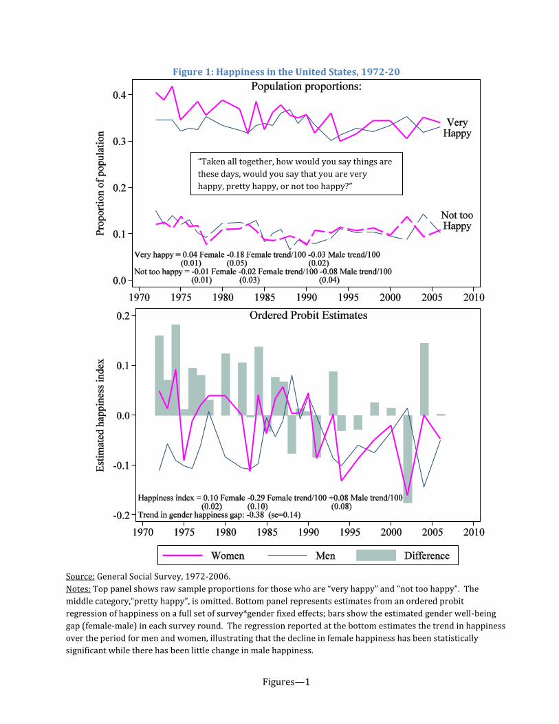
Figures—1

Figure 1: Happiness in the United States, 1972-20

Source: General Social Survey, 1972-2006.

Notes: Top panel shows raw sample proportions for those who are “very happy” and “not too happy”. The

middle category,“pretty happy”, is omitted. Bottom panel represents estimates from an ordered probit

regression of happiness on a full set of survey*gender fixed effects; bars show the estimated gender well-being

gap (female-male) in each survey round. The regression reported at the bottom estimates the trend in happiness

over the period for men and women, illustrating that the decline in female happiness has been statistically

significant while there has been little change in male happiness.

“Taken all together, how would you say things are

these days, would you say that you are very

happy, pretty happy, or not too happy?”

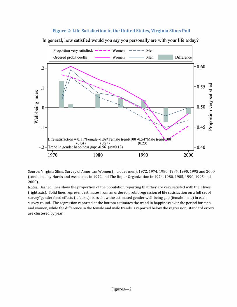
Figures—2

Figure 2: Life Satisfaction in the United States, Virginia Slims Poll

Source: Virginia Slims Survey of American Women (includes men), 1972, 1974, 1980, 1985, 1990, 1995 and 2000

(conducted by Harris and Associates in 1972 and The Roper Organization in 1974, 1980, 1985, 1990, 1995 and

2000).

Notes: Dashed lines show the proportion of the population reporting that they are very satisfed with their lives

(right axis). Solid lines represent estimates from an ordered probit regression of life satisfaction on a full set of

survey*gender fixed effects (left axis); bars show the estimated gender well-being gap (female-male) in each

survey round. The regression reported at the bottom estimates the trend in happiness over the period for men

and women, while the difference in the female and male trends is reported below the regression; standard errors

are clustered by year.

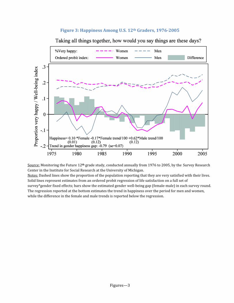
Figures—3

Figure 3: Happiness Among U.S. 12th Graders, 1976-2005

Source: Monitoring the Future 12th grade study, conducted annually from 1976 to 2005, by the Survey Research

Center in the Institute for Social Research at the University of Michigan.

Notes: Dashed lines show the proportion of the population reporting that they are very satisfied with their lives.

Solid lines represent estimates from an ordered probit regression of life satisfaction on a full set of

survey*gender fixed effects; bars show the estimated gender well-being gap (female-male) in each survey round.

The regression reported at the bottom estimates the trend in happiness over the period for men and women,

while the difference in the female and male trends is reported below the regression.

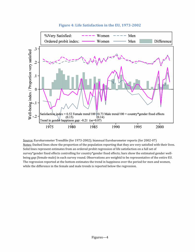
Figures—4

Figure 4: Life Satisfaction in the EU, 1973-2002

Source: Eurobarometer Trendfile (for 1973-2002); biannual Eurobarometer reports (for 2002-07)

Notes: Dashed lines show the proportion of the population reporting that they are very satisfied with their lives.

Solid lines represent estimates from an ordered probit regression of life satisfaction on a full set of

survey*gender fixed effects controlling for country*gender fixed effects; bars show the estimated gender well-

being gap (female-male) in each survey round. Observations are weightd to be representative of the entire EU.

The regression reported at the bottom estimates the trend in happiness over the period for men and women,

while the difference in the female and male trends is reported below the regression.

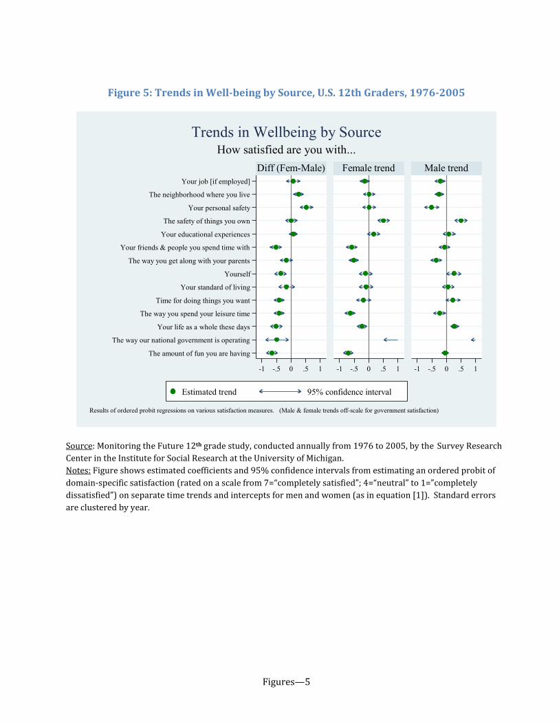
Figures—5

Figure 5: Trends in Well-being by Source, U.S. 12th Graders, 1976-2005

Source: Monitoring the Future 12th grade study, conducted annually from 1976 to 2005, by the Survey Research

Center in the Institute for Social Research at the University of Michigan.

Notes: Figure shows estimated coefficients and 95% confidence intervals from estimating an ordered probit of

domain-specific satisfaction (rated on a scale from 7=“completely satisfied”; 4=“neutral” to 1=”completely

dissatisfied”) on separate time trends and intercepts for men and women (as in equation [1]). Standard errors

are clustered by year.

Your job [if employed]

The neighborhood where you live

Your personal safety

The safety of things you own

Your educational experiences

Your friends & people you spend time with

The way you get along with your parents

Yourself

Your standard of living

Time for doing things you want

The way you spend your leisure time

Your life as a whole these days

The way our national government is operating

The amount of fun you are having

-1 -.5 0 .5 1 -1 -.5 0 .5 1 -1 -.5 0 .5 1

Diff (Fem-Male) Female trend Male trend

Estimated trend 95% confidence interval

Results of ordered probit regressions on various satisfaction measures. (Male & female trends off-scale for government satisfaction)

How satisfied are you with...

Trends in Wellbeing by Source

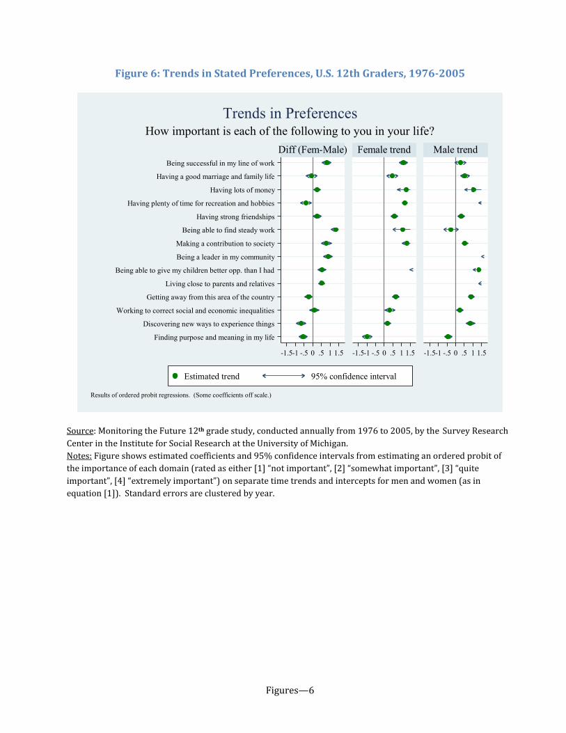
Figures—6

Figure 6: Trends in Stated Preferences, U.S. 12th Graders, 1976-2005

Source: Monitoring the Future 12th grade study, conducted annually from 1976 to 2005, by the Survey Research

Center in the Institute for Social Research at the University of Michigan.

Notes: Figure shows estimated coefficients and 95% confidence intervals from estimating an ordered probit of

the importance of each domain (rated as either [1] “not important”, [2] “somewhat important”, [3] “quite

important”, [4] “extremely important”) on separate time trends and intercepts for men and women (as in

equation [1]). Standard errors are clustered by year.

Being successful in my line of work

Having a good marriage and family life

Having lots of money

Having plenty of time for recreation and hobbies

Having strong friendships

Being able to find steady work

Making a contribution to society

Being a leader in my community

Being able to give my children better opp. than I had

Living close to parents and relatives

Getting away from this area of the country

Working to correct social and economic inequalities

Discovering new ways to experience things

Finding purpose and meaning in my life

-1.5-1 -.5 0 .5 1 1.5 -1.5-1 -.5 0 .5 1 1.5 -1.5-1 -.5 0 .5 1 1.5

Diff (Fem-Male) Female trend Male trend

Estimated trend 95% confidence interval

Results of ordered probit regressions. (Some coefficients off scale.)

How important is each of the following to you in your life?

Trends in Preferences

Figures—7

Figure 7: U.S. Suicide Rates, by Gender

Source: Suicide data for 1950–1998 are from National Center for Health Statistics report “Vital Statistics: Mortality, Vol. 2.” Data from 1999–2005 have been downloaded from the Center for Disease Control’s Wonder system which accesses the NCHS “Compressed Mortality Files” (http://wonder.cdc.gov/). Notes: Series breaks correspond with changing ICD codes.

Suicide Rates in the United States

0

5

10

15

20

25

1950 1955 1960 1965 1970 1975 1980 1985 1990 1995 2000 2005

An

nu

al s

uic

ide

s p

er

10

0,0

00

pe

op

le;

ag

e-a

dju

ste

d .

0.20

0.24

0.28

0.32

0.36

0.40

Male

Female

Ratio: Female-to-Male

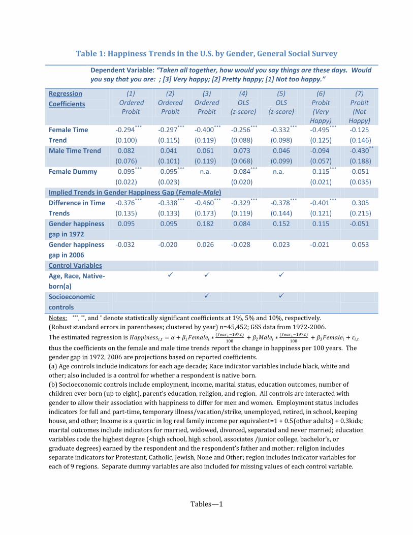
Tables—1

Table 1: Happiness Trends in the U.S. by Gender, General Social Survey

Dependent Variable: “Taken all together, how would you say things are these days. Would you say that you are: ; [3] Very happy; [2] Pretty happy; [1] Not too happy.”

Regression

Coefficients

(1) Ordered

Probit

(2) Ordered Probit

(3) Ordered Probit

(4) OLS

(z-score)

(5) OLS

(z-score)

(6) Probit (Very

Happy)

(7) Probit (Not

Happy) Female Time

Trend

-0.294***

(0.100)

-0.297***

(0.115)

-0.400***

(0.119)

-0.256***

(0.088)

-0.332***

(0.098)

-0.495***

(0.125)

-0.125

(0.146)

Male Time Trend 0.082

(0.076)

0.041

(0.101)

0.061

(0.119)

0.073

(0.068)

0.046

(0.099)

-0.094

(0.057)

-0.430**

(0.188)

Female Dummy 0.095***

(0.022)

0.095***

(0.023)

n.a. 0.084***

(0.020)

n.a. 0.115***

(0.021)

-0.051

(0.035)

Implied Trends in Gender Happiness Gap (Female-Male)

Difference in Time

Trends

-0.376***

(0.135)

-0.338***

(0.133)

-0.460***

(0.173)

-0.329***

(0.119)

-0.378***

(0.144)

-0.401***

(0.121)

0.305

(0.215)

Gender happiness

gap in 1972

0.095 0.095 0.182 0.084 0.152 0.115 -0.051

Gender happiness

gap in 2006

-0.032 -0.020 0.026 -0.028 0.023 -0.021 0.053

Control Variables

Age, Race, Native-

born(a)

Socioeconomic

controls

Notes: ***, **, and * denote statistically significant coefficients at 1%, 5% and 10%, respectively.

(Robust standard errors in parentheses; clustered by year) n=45,452; GSS data from 1972-2006.

The estimated regression is 𝐻𝑎𝑝𝑝𝑖𝑛𝑒𝑠𝑠𝑖,𝑡 = 𝛼 + 𝛽1𝐹𝑒𝑚𝑎𝑙𝑒𝑖 ∗(𝑌𝑒𝑎𝑟 𝑡−1972)

100 + 𝛽2𝑀𝑎𝑙𝑒𝑖 ∗

(𝑌𝑒𝑎𝑟 𝑡−1972)

100 + 𝛽3𝐹𝑒𝑚𝑎𝑙𝑒𝑖 + 𝜀𝑖 ,𝑡

thus the coefficients on the female and male time trends report the change in happiness per 100 years. The

gender gap in 1972, 2006 are projections based on reported coefficients.

(a) Age controls include indicators for each age decade; Race indicator variables include black, white and

other; also included is a control for whether a respondent is native born.

(b) Socioeconomic controls include employment, income, marital status, education outcomes, number of

children ever born (up to eight), parent’s education, religion, and region. All controls are interacted with

gender to allow their association with happiness to differ for men and women. Employment status includes

indicators for full and part-time, temporary illness/vacation/strike, unemployed, retired, in school, keeping

house, and other; Income is a quartic in log real family income per equivalent=1 + 0.5(other adults) + 0.3kids;

marital outcomes include indicators for married, widowed, divorced, separated and never married; education

variables code the highest degree (<high school, high school, associates /junior college, bachelor’s, or

graduate degrees) earned by the respondent and the respondent’s father and mother; religion includes

separate indicators for Protestant, Catholic, Jewish, None and Other; region includes indicator variables for

each of 9 regions. Separate dummy variables are also included for missing values of each control variable.

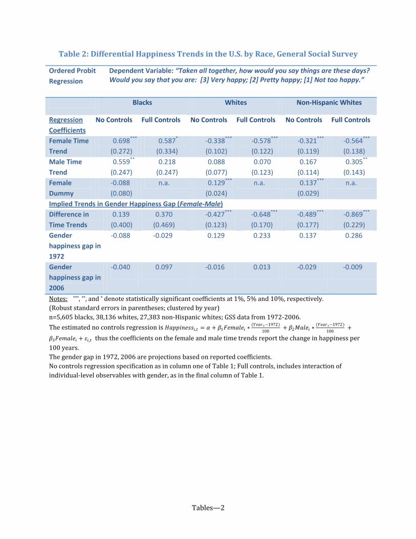
Tables—2

Table 2: Differential Happiness Trends in the U.S. by Race, General Social Survey

Ordered Probit

Regression

Dependent Variable: “Taken all together, how would you say things are these days? Would you say that you are: [3] Very happy; [2] Pretty happy; [1] Not too happy.”

Blacks Whites Non-Hispanic Whites

Regression

Coefficients

No Controls Full Controls No Controls Full Controls No Controls Full Controls

Female Time

Trend

0.698***

(0.272)

0.587*

(0.334)

-0.338***

(0.102)

-0.578***

(0.122)

-0.321***

(0.119)

-0.564***

(0.138)

Male Time

Trend

0.559**

(0.247)

0.218

(0.247)

0.088

(0.077)

0.070

(0.123)

0.167

(0.114)

0.305**

(0.143)

Female

Dummy

-0.088

(0.080)

n.a. 0.129***

(0.024)

n.a. 0.137***

(0.029)

n.a.

Implied Trends in Gender Happiness Gap (Female-Male)

Difference in

Time Trends

0.139

(0.400)

0.370

(0.469)

-0.427***

(0.123)

-0.648***

(0.170)

-0.489***

(0.177)

-0.869***

(0.229)

Gender

happiness gap in

1972

-0.088 -0.029 0.129 0.233 0.137 0.286

Gender

happiness gap in

2006

-0.040 0.097 -0.016 0.013 -0.029 -0.009

Notes: ***, **, and * denote statistically significant coefficients at 1%, 5% and 10%, respectively.

(Robust standard errors in parentheses; clustered by year)

n=5,605 blacks, 38,136 whites, 27,383 non-Hispanic whites; GSS data from 1972-2006.

The estimated no controls regression is 𝐻𝑎𝑝𝑝𝑖𝑛𝑒𝑠𝑠𝑖,𝑡 = 𝛼 + 𝛽1𝐹𝑒𝑚𝑎𝑙𝑒𝑖 ∗(𝑌𝑒𝑎𝑟 𝑡−1972)

100 + 𝛽2𝑀𝑎𝑙𝑒𝑖 ∗

(𝑌𝑒𝑎𝑟 𝑡−1972)

100 +

𝛽3𝐹𝑒𝑚𝑎𝑙𝑒𝑖 + 𝜀𝑖,𝑡

thus the coefficients on the female and male time trends report the change in happiness per

100 years.

The gender gap in 1972, 2006 are projections based on reported coefficients.

No controls regression specification as in column one of Table 1; Full controls, includes interaction of

individual-level observables with gender, as in the final column of Table 1.

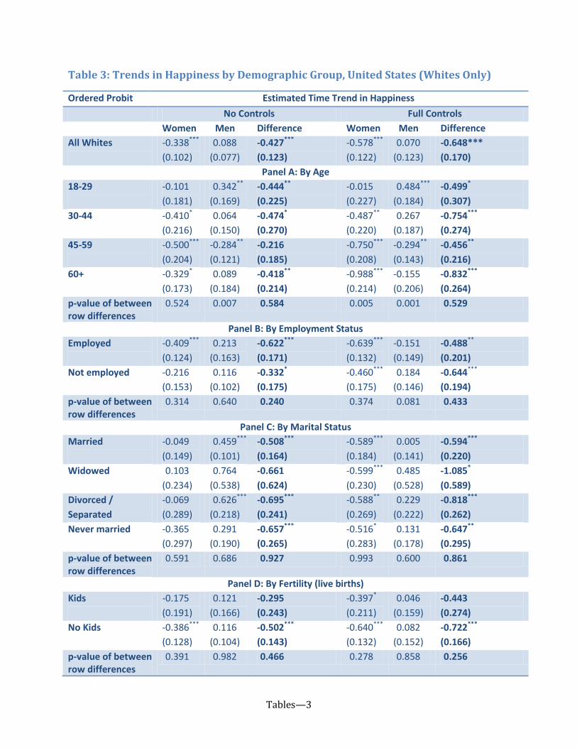
Tables—3

Table 3: Trends in Happiness by Demographic Group, United States (Whites Only)

Ordered Probit Estimated Time Trend in Happiness

No Controls Full Controls

Women Men Difference Women Men Difference

All Whites

-0.338***

(0.102)

0.088

(0.077)

-0.427***

(0.123)

-0.578***

(0.122)

0.070

(0.123)

-0.648***

(0.170)

Panel A: By Age

18-29

-0.101

(0.181)

0.342**

(0.169)

-0.444**

(0.225)

-0.015

(0.227)

0.484***

(0.184)

-0.499*

(0.307)

30-44

-0.410*

(0.216)

0.064

(0.150)

-0.474*

(0.270)

-0.487**

(0.220)

0.267

(0.187)

-0.754***

(0.274)

45-59

-0.500***

(0.204)

-0.284**

(0.121)

-0.216

(0.185)

-0.750***

(0.208)

-0.294**

(0.143)

-0.456**

(0.216)

60+

-0.329*

(0.173)

0.089

(0.184)

-0.418**

(0.214)

-0.988***

(0.214)

-0.155

(0.206)

-0.832***

(0.264)

p-value of between row differences

0.524 0.007 0.584 0.005 0.001 0.529

Panel B: By Employment Status

Employed

-0.409***

(0.124)

0.213

(0.163)

-0.622***

(0.171)

-0.639***

(0.132)

-0.151

(0.149)

-0.488**

(0.201)

Not employed

-0.216

(0.153)

0.116

(0.102)

-0.332*

(0.175)

-0.460***

(0.175)

0.184

(0.146)

-0.644***

(0.194)

p-value of between row differences

0.314 0.640 0.240 0.374 0.081 0.433

Panel C: By Marital Status

Married

-0.049

(0.149)

0.459***

(0.101)

-0.508***

(0.164)

-0.589***

(0.184)

0.005

(0.141)

-0.594***

(0.220)

Widowed

0.103

(0.234)

0.764

(0.538)

-0.661

(0.624)

-0.599***

(0.230)

0.485

(0.528)

-1.085*

(0.589)

Divorced /

Separated

-0.069

(0.289)

0.626***

(0.218)

-0.695***

(0.241)

-0.588**

(0.269)

0.229

(0.222)

-0.818***

(0.262)

Never married

-0.365

(0.297)

0.291

(0.190)

-0.657***

(0.265)

-0.516*

(0.283)

0.131

(0.178)

-0.647**

(0.295)

p-value of between row differences

0.591 0.686 0.927 0.993 0.600 0.861

Panel D: By Fertility (live births)

Kids

-0.175

(0.191)

0.121

(0.166)

-0.295

(0.243)

-0.397*

(0.211)

0.046

(0.159)

-0.443

(0.274)

No Kids

-0.386***

(0.128)

0.116

(0.104)

-0.502***

(0.143)

-0.640***

(0.132)

0.082

(0.152)

-0.722***

(0.166)

p-value of between row differences

0.391 0.982 0.466 0.278 0.858 0.256

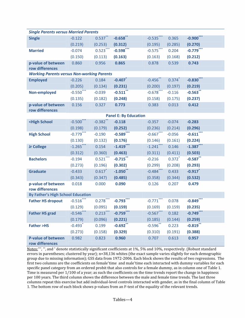
Tables—4

Single Parents versus Married Parents

Single

-0.122

(0.219)

0.537**

(0.253)

-0.658**

(0.312)

-0.535***

(0.195)

0.365

(0.285)

-0.900***

(0.270)

Married

-0.074

(0.150)

0.523***

(0.113)

-0.598***

(0.163)

-0.575***

(0.163)

0.204

(0.168)

-0.779***

(0.212)

p-value of between row differences

0.860 0.956 0.865 0.878 0.539 0.743

Working Parents versus Non-working Parents

Employed

-0.226

(0.205)

0.184

(0.134)

-0.407*

(0.231)

-0.456**

(0.200)

0.374*

(0.197)

-0.830***

(0.219)

Non-employed

-0.550***

(0.135)

-0.039

(0.182)

-0.511**

(0.248)

-0.678***

(0.158)

-0.116

(0.175)

-0.563**

(0.237)

p-value of between row differences

0.156 0.327 0.773 0.383 0.013 0.412

Panel E: By Education

<High School

-0.500***

(0.198)

-0.382**

(0.179)

-0.118

(0.252)

-0.357

(0.236)

-0.074

(0.214)

-0.283

(0.296)

High School

-0.779***

(0.130)

-0.190

(0.132)

-0.589***

(0.176)

-0.667***

(0.146)

-0.056

(0.161)

-0.611***

(0.224)

Jr College

-1.265***

(0.312)

0.154

(0.360)

-1.419***

(0.463)

-1.241***

(0.311)

0.146

(0.411)

-1.387***

(0.503)

Bachelors

-0.194

(0.273)

0.521***

(0.196)

-0.715**

(0.302)

-0.216

(0.299)

0.372*

(0.208)

-0.587**

(0.293)

Graduate

-0.433

(0.343)

0.617*

(0.347)

-1.050**

(0.485)

-0.484***

(0.358)

0.433

(0.344)

-0.917*

(0.532)

p-value of between row differences

0.018 0.000 0.090 0.126 0.207 0.479

By Father’s High School Education

Father HS dropout

-0.516***

(0.129)

0.278***

(0.095)

-0.793***

(0.159)

-0.771***

(0.169)

0.078

(0.159)

-0.849***

(0.235)

Father HS grad

-0.546***

(0.179)

0.213***

(0.096)

-0.759***

(0.221)

-0.567***

(0.185)

0.182

(0.144)

-0.749***

(0.259)

Father >HS

-0.493*

(0.273)

0.199

(0.158)

-0.692**

(0.329)

-0.596**

(0.310)

0.223

(0.191)

-0.819**

(0.388)

P-value of between row differences

0.982 0.823 0.960 0.707 0.613 0.957

Notes:***, **, and * denote statistically significant coefficients at 1%, 5% and 10%, respectively. (Robust standard errors in parentheses; clustered by year); n=38,136 whites (the exact sample varies slightly for each demographic group due to missing information); GSS data from 1972-2006. Each block shows the results of two regressions. The first two columns are the coefficients on female*time and male*time each interacted with dummy variables for each specific panel category from an ordered probit that also controls for a female dummy, as in column one of Table 1. Time is measured per 1/100 of a year; as such the coefficients on the time trends report the change in happiness per 100 years. The third column shows the difference between the male and female time trends. The last three columns repeat this exercise but add individual-level controls interacted with gender, as in the final column of Table 1. The bottom row of each block shows p-values from an F-test of the equality of the relevant trends.

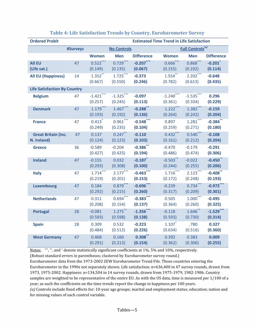
Tables—5

Table 4: Life Satisfaction Trends by Country, Eurobarometer Survey

Ordered Probit Estimated Time Trend in Life Satisfaction

#Surveys No Controls Full Controls(a)

Women Men Difference Women Men Difference

All EU (Life sat.)

47 0.522*** (0.149)

0.729*** (0.135)

-0.207*** (0.067)

0.666*** (0.155)

0.868*** (0.192)

-0.201* (0.114)

All EU (Happiness) 14 1.352** (0.667)

1.725*** (0.550)

-0.373 (0.246)

1.554** (0.782)

2.202*** (0.613)

-0.648 (0.435)

Life Satisfaction By Country

Belgium 47 -1.421*** (0.257)

-1.325*** (0.245)

-0.097 (0.113)

-1.240*** (0.361)

-1.535*** (0.334)

0.296 (0.229)

Denmark 47 1.179*** (0.193)

1.467*** (0.192)

-0.288** (0.136)

1.222*** (0.264)

1.382*** (0.242)

-0.159 (0.204)

France 47 0.413* (0.249)

0.961*** (0.235)

-0.548*** (0.104)

0.897 (0.259)

1.281*** (0.271)

-0.384** (0.180)

Great Britain (inc. N. Ireland)

47 0.137 (0.124)

0.247** (0.123)

-0.110 (0.103)

0.432*** (0.161)

0.540*** (0.212)

-0.108 (0.204)

Greece 36 -0.589 (0.427)

-0.204 (0.425)

-0.386** (0.194)

-0.470 (0.486)

-0.179 (0.474)

-0.291 (0.306)

Ireland 47 -0.155 (0.293)

0.032 (0.308)

-0.187* (0.100)

-0.503** (0.244)

-0.022 (0.255)

-0.450** (0.206)

Italy 47 1.714*** (0.219)

2.177*** (0.201)

-0.463*** (0.153)

1.716*** (0.172)

2.123*** (0.248)

-0.408** (0.193)

Luxembourg 47 0.184 (0.292)

0.879*** (0.215)

-0.696*** (0.260)

-0.239 (0.317)

0.734*** (0.209)

-0.972*** (0.301)

Netherlands 47 0.311 (0.208)

0.694*** (0.154)

-0.383*** (0.137)

0.505 (0.364)

1.000*** (0.260)

-0.495 (0.325)

Portugal 28 -0.081 (0.593)

1.275** (0.598)

-1.356*** (0.138)

-0.118 (0.593)

1.646** (0.730)

-1.529*** (0.314)

Spain 28 0.309 (0.484)

0.532 (0.512)

-0.223 (0.226)

1.107* (0.634)

.780 (0.516)

0.327 (0.360)

West Germany 47 0.468 (0.291)

0.160 (0.213)

0.308** (0.154)

0.392 (0.362)

0.383 (0.306)

0.009 (0.255)

Notes: ***, **, and * denote statistically significant coefficients at 1%, 5% and 10%, respectively.

(Robust standard errors in parentheses; clustered by Eurobarometer survey round.)

Eurobarometer data from the 1973-2002 ZEW Eurobarometer Trend File. Those countries entering the

Eurobarometer in the 1990s not separately shown. Life satisfaction: n=636,400 in 47 survey rounds, drawn from

1973, 1975-2002. Happiness: n=134,504 in 14 survey rounds, drawn from 1975-1979, 1982-1986. Country

samples are weighted to be representative of the entire EU. As with the US data, time is measured per 1/100 of a

year; as such the coefficients on the time trends report the change in happiness per 100 years.

(a) Controls include fixed effects for: 10-year age groups; marital and employment status; education; nation and

for missing values of each control variable.

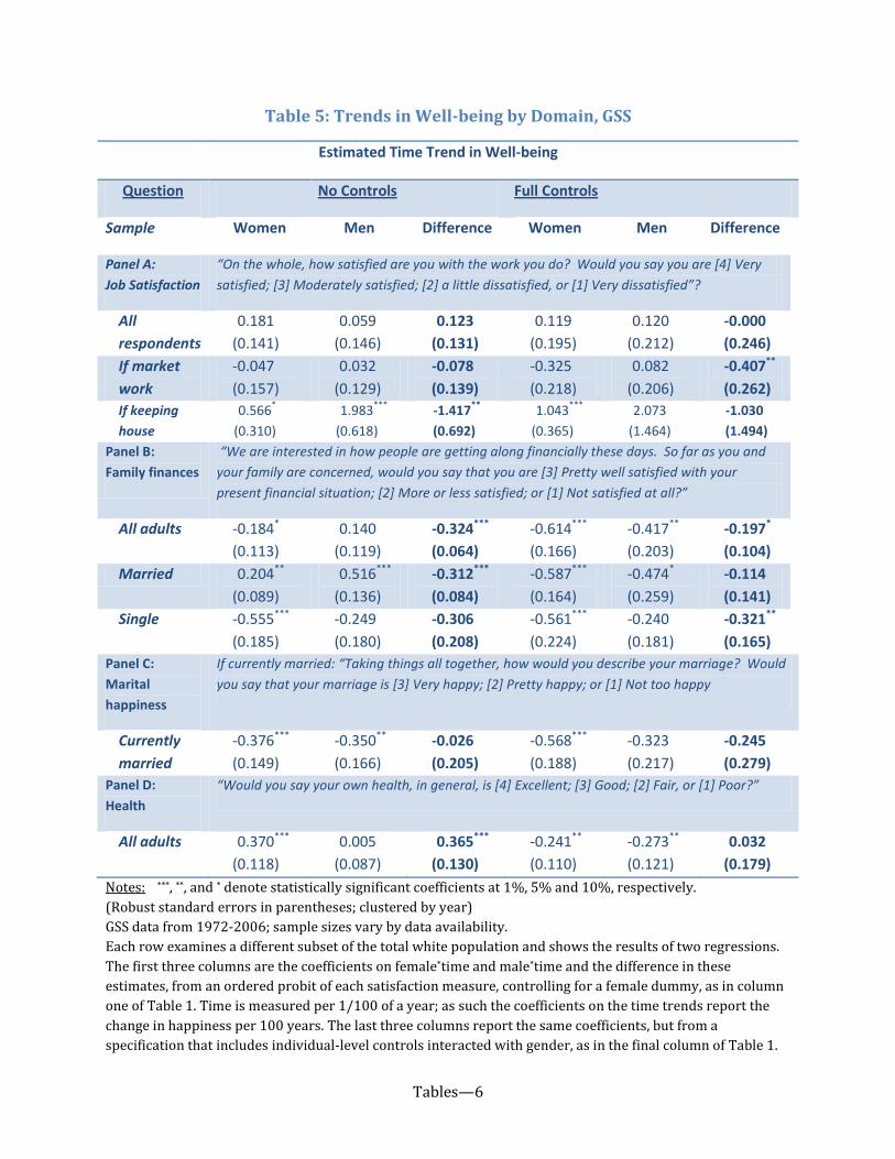
Tables—6

Table 5: Trends in Well-being by Domain, GSS

Estimated Time Trend in Well-being

Question No Controls Full Controls

Sample Women Men Difference Women Men Difference

Panel A:

Job Satisfaction

“On the whole, how satisfied are you with the work you do? Would you say you are [4] Very

satisfied; [3] Moderately satisfied; [2] a little dissatisfied, or [1] Very dissatisfied”?

All

respondents

0.181

(0.141)

0.059

(0.146)

0.123

(0.131)

0.119

(0.195)

0.120

(0.212)

-0.000

(0.246)

If market

work

-0.047

(0.157)

0.032

(0.129)

-0.078

(0.139)

-0.325

(0.218)

0.082

(0.206)

-0.407**

(0.262)

If keeping

house

0.566*

(0.310)

1.983***

(0.618)

-1.417**

(0.692)

1.043***

(0.365)

2.073

(1.464)

-1.030

(1.494)

Panel B:

Family finances

“We are interested in how people are getting along financially these days. So far as you and

your family are concerned, would you say that you are [3] Pretty well satisfied with your

present financial situation; [2] More or less satisfied; or [1] Not satisfied at all?”

All adults -0.184*

(0.113)

0.140

(0.119)

-0.324***

(0.064)

-0.614***

(0.166)

-0.417**

(0.203)

-0.197*

(0.104)

Married 0.204**

(0.089)

0.516***

(0.136)

-0.312***

(0.084)

-0.587***

(0.164)

-0.474*

(0.259)

-0.114

(0.141)

Single -0.555***

(0.185)

-0.249

(0.180)

-0.306

(0.208)

-0.561***

(0.224)

-0.240

(0.181)

-0.321**

(0.165)

Panel C:

Marital

happiness

If currently married: “Taking things all together, how would you describe your marriage? Would

you say that your marriage is [3] Very happy; [2] Pretty happy; or [1] Not too happy

Currently

married

-0.376***

(0.149)

-0.350**

(0.166)

-0.026

(0.205)

-0.568***

(0.188)

-0.323

(0.217)

-0.245

(0.279)

Panel D:

Health

“Would you say your own health, in general, is [4] Excellent; [3] Good; [2] Fair, or [1] Poor?”

All adults 0.370***

(0.118)

0.005

(0.087)

0.365***

(0.130)

-0.241**

(0.110)

-0.273**

(0.121)

0.032

(0.179)

Notes: ***, **, and * denote statistically significant coefficients at 1%, 5% and 10%, respectively.

(Robust standard errors in parentheses; clustered by year)

GSS data from 1972-2006; sample sizes vary by data availability.

Each row examines a different subset of the total white population and shows the results of two regressions.

The first three columns are the coefficients on female*time and male*time and the difference in these

estimates, from an ordered probit of each satisfaction measure, controlling for a female dummy, as in column

one of Table 1. Time is measured per 1/100 of a year; as such the coefficients on the time trends report the

change in happiness per 100 years. The last three columns report the same coefficients, but from a

specification that includes individual-level controls interacted with gender, as in the final column of Table 1.

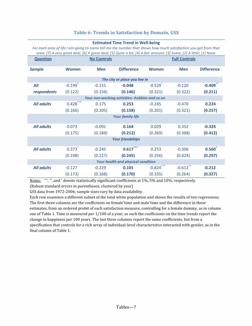
Tables—7

Table 6: Trends in Satisfaction by Domain, GSS

Estimated Time Trend in Well-being

For each area of life I am going to name tell me the number that shows how much satisfaction you get from that area: [7] A very great deal; [6] A great deal; [5] Quite a bit; [4] A fair amount; [3] Some; [2] A little; [1] None

Question No Controls Full Controls

Sample Women Men Difference Women Men Difference

The city or place you live in

All

respondents

-0.199*

(0.122)

-0.151

(0.156)

-0.048

(0.146)

-0.529*

(0.321)

-0.120

(0.322)

-0.409**

(0.211)

Your non-working activities--hobbies and so on

All adults 0.428***

(0.166)

0.175

(0.205)

0.253

(0.158)

-0.245

(0.201)

-0.470

(0.321)

0.224

(0.257)

Your family life

All adults 0.073

(0.175)

-0.091

(0.184)

0.164

(0.212)

0.029

(0.269)

0.352

(0.368)

-0.324

(0.412)

Your friendships

All adults 0.373*

(0.198)

-0.245

(0.227)

0.617***

(0.245)

0.253

(0.256)

-0.306

(0.424)

0.560*

(0.297)

Your health and physical condition

All adults -0.127

(0.173)

-0.229

(0.168)

0.101

(0.170)

-0.824***

(0.335)

-0.612**

(0.264)

-0.212

(0.327)

Notes: ***, **, and * denote statistically significant coefficients at 1%, 5% and 10%, respectively.

(Robust standard errors in parentheses; clustered by year)

GSS data from 1972-2006; sample sizes vary by data availability.

Each row examines a different subset of the total white population and shows the results of two regressions.

The first three columns are the coefficients on female*time and male*time and the difference in these

estimates, from an ordered probit of each satisfaction measure, controlling for a female dummy, as in column

one of Table 1. Time is measured per 1/100 of a year; as such the coefficients on the time trends report the

change in happiness per 100 years. The last three columns report the same coefficients, but from a

specification that controls for a rich array of individual-level characteristics interacted with gender, as in the

final column of Table 1.