The Particle World of Condensed Matter - IFW · PDF fileThe Particle World of Condensed Matter H. Eschrig ... This project was also triggered ... electro-dynamical Hamiltonian

The Particle World of Condensed

Matter

H. EschrigIFW Dresden and

Dresden University of TechnologyGermany

Preface

Science in our days gets more and more specialized, and often even the actors indifferent fields of the same discipline do not find a common language any more.Horizons narrow with the danger of ending up in ‘provincialism in the space ofknowledge’. On the other hand, probably the most appropriate characterization ofphysics as a discipline is the aim of a unified understanding of nature. From timeto time chains of events appear in physics where this unified approach shines upin a bright spotlight on the scene, and then again it drops out of the focus in thehard work of solving complex tasks.

Such a splendid period of mounting a peak and widening the horizon fromday to day were the fifties and early sixties of twentieth century in quantum fieldtheory with that fascinating cross-fertilization between Elementary Particle andSolid State Physics. On the side of Solid State Theory it layed the ground for thequasi-particle approach, so successful during the sixties and seventies. After a kindof stock taking and putting more emphasis on the limitations of this approach,which of course exist and have to be taken into consideration, in recent time newkinds of exotic quasi-particles were discovered and the whole approach has by nomeans lost its topicality, proving the vivid potentials of field theory.

In the middle of the eighties, Musik Kaganov and myself started a review projectfocusing on the underlying principles and the deeper understanding of the approach.This project was also triggered (at least as regards me) by our feeling in discussionwith colleagues that quite not all of them were well aware of those underlyingprinciples which we consider fundamental to the Theory of Solids. Then, thepolitical changes came in Germany demanding a larger effort on my side in thereorganization of research in its eastern part, and Musik left Russia in 1994. Theproject remained unfinished.

In the summer term 2004, I read a three-hours one-term introductory course inField Theory for the Solid State, and in preparing for it I came back to the matter aswe left it in 1988. Although I now had to revise and finish the text without Musik,it is of course further on in large parts inspired by him. (The reader consultingpublications by M. I. Kaganov will find out in which parts in particular.) Sincewe did not have a chance to discuss the result in detail, we agreed that I shouldnow present the text as a single author. Particularly, I am now responsible for the

6 Preface

overall style of presentation, and, of course, for all errors. The text would, however,never have been accomplished without the long period of our discussions and thehonor and delight of a life-long friendship with Musik Kaganov.

Dresden, November 2004 Helmut Eschrig

Contents

Introduction 9

1 Technical Tools 13

1.1 Resume on N -Particle Quantum States . . . . . . . . . . . . . . . . . . . 131.1.1 Schrodinger Representation . . . . . . . . . . . . . . . . . . . . . . 151.1.2 Spin . . . . . . . . . . . . . . . . . . . . . . . . . . . . . . . . . . . 181.1.3 Momentum Representation . . . . . . . . . . . . . . . . . . . . . . 241.1.4 Heisenberg Representation . . . . . . . . . . . . . . . . . . . . . . 281.1.5 Hartree-Fock Theory . . . . . . . . . . . . . . . . . . . . . . . . . 29

1.2 The Fock Space . . . . . . . . . . . . . . . . . . . . . . . . . . . . . . . . 331.2.1 Occupation Number Representation . . . . . . . . . . . . . . . . . 351.2.2 Coherent Bosonic States . . . . . . . . . . . . . . . . . . . . . . . 381.2.3 Grassmann Numbers . . . . . . . . . . . . . . . . . . . . . . . . . 421.2.4 Coherent Fermionic States . . . . . . . . . . . . . . . . . . . . . . 44

1.3 Field Quantization . . . . . . . . . . . . . . . . . . . . . . . . . . . . . . . 471.3.1 Locality . . . . . . . . . . . . . . . . . . . . . . . . . . . . . . . . . 491.3.2 Superselection . . . . . . . . . . . . . . . . . . . . . . . . . . . . . 50

2 Macroscopic Quantum Systems 55

2.1 Thermodynamic Limit . . . . . . . . . . . . . . . . . . . . . . . . . . . . 552.2 Pure and Mixed Quantum States . . . . . . . . . . . . . . . . . . . . . . 592.3 Thermodynamic States . . . . . . . . . . . . . . . . . . . . . . . . . . . . 642.4 Stationary States . . . . . . . . . . . . . . . . . . . . . . . . . . . . . . . 67

3 Quasi-Stationary Excitations 72

3.1 Pictures . . . . . . . . . . . . . . . . . . . . . . . . . . . . . . . . . . . . . 723.2 Time-dependent Green’s Functions . . . . . . . . . . . . . . . . . . . . . 753.3 Non-Interacting Particles . . . . . . . . . . . . . . . . . . . . . . . . . . . 783.4 Interacting Systems . . . . . . . . . . . . . . . . . . . . . . . . . . . . . . 813.5 Density of States . . . . . . . . . . . . . . . . . . . . . . . . . . . . . . . . 853.6 Collective Excitations . . . . . . . . . . . . . . . . . . . . . . . . . . . . . 873.7 Non-Zero Temperatures . . . . . . . . . . . . . . . . . . . . . . . . . . . . 90

8 Contents

4 Model Hamiltonians 95

4.1 Non-Interacting Particles, T = 0 . . . . . . . . . . . . . . . . . . . . . . . 954.2 Non-Interacting Particles, T > 0 . . . . . . . . . . . . . . . . . . . . . . . 1004.3 BCS Theory . . . . . . . . . . . . . . . . . . . . . . . . . . . . . . . . . . 1044.4 Weakly Interacting Bose Gas . . . . . . . . . . . . . . . . . . . . . . . . . 1074.5 Discussion of the Model Approach . . . . . . . . . . . . . . . . . . . . . . 110

5 Quasi-Particles 114

5.1 Landau’s Quasi-Particle Conception . . . . . . . . . . . . . . . . . . . . . 1155.2 Quasi-Particles in a Crystalline Solid . . . . . . . . . . . . . . . . . . . . 1185.3 Green’s Function of Bloch Electrons . . . . . . . . . . . . . . . . . . . . . 1215.4 Green’s Function of Lattice Phonons . . . . . . . . . . . . . . . . . . . . 1255.5 Disordered Systems . . . . . . . . . . . . . . . . . . . . . . . . . . . . . . 1285.6 Frontiers of the Quasi-Particle Picture . . . . . . . . . . . . . . . . . . . . 131

6 The Nature of the Vacuum 134

6.1 Spontaneous Symmetry Breaking . . . . . . . . . . . . . . . . . . . . . . 1346.2 Gauge Symmetry . . . . . . . . . . . . . . . . . . . . . . . . . . . . . . . 1376.3 Anomalous Mean Values . . . . . . . . . . . . . . . . . . . . . . . . . . . 1396.4 Goldstone and Higgs Modes . . . . . . . . . . . . . . . . . . . . . . . . . 143

7 What Matter Consists of 146

7.1 The Hierarchy of Hamiltonians . . . . . . . . . . . . . . . . . . . . . . . . 1477.2 ‘From the First Principles’ . . . . . . . . . . . . . . . . . . . . . . . . . . 148

8 Epilogue: The Unifying Picture of Physics 151

Appendices 154

A I Self-energy operator . . . . . . . . . . . . . . . . . . . . . . . . . . . . . . 154A II Density functional theory . . . . . . . . . . . . . . . . . . . . . . . . . . . 155

Bibliography 160

Index 170

Introduction

The idea of quasi-particles has turned out to be one of the most profound andfundamental ideas in the quantum theory of condensed matter. In terms ofphonons, magnons, excitons, conduction electrons and holes and so on, the wholeof experimental data and theoretical predictions related to the most various solidsunder the most different conditions is described. In recent years, a whole zoo of newquasi-particles emerged as composite fermions, spinons, holons, orbitons, phasons,and others. The fertility of solid state research to give birth to new quasi-particlesseems not to diminish after five decades.

There are different understandings of quasi-particles. To the one, the quasi-particles serve as a simple approach replacing the ‘true’ theory by the primitiveone-particle approximation. To the other it is the ‘remedy from all diseases’: thequasi-particles (in their opinion) are capable of describing everything that is goingon in a piece of condensed matter, thereby, if something is not yet described bythem, it certainly will be in future. . . One of the goals of the present text is tryingto show the true place of quasi-particles (and of particles too) in modern physics.

The macroscopicity (the practically infinite number of microscopic degrees offreedom) of any solid not only introduces specific computational techniques—it also forms the fundamental ideas. So, while for micro-objects (atoms, ions,small molecules) the basic task consists of determining their energy spectra, i.e.the set of stationary states, for a macroscopic, condensed system the basic taskconsists of defining and determining the quasi-stationary states describing quasi-particles which, with rare exceptions, have finite lifetimes. Here, a consequentcomputational way of mathematically extracting the quasi-particles literally fromthe ‘first principles’ does not exist. Strictly speaking, even the correspondingproblem cannot be formulated, for up to now we do not know the true elementarybeings matter consists of (if there is at all such a last pre-matter). Also not goinginto such theoretical depths and assuming that any solid consists of nuclei andelectrons, it is not possible by means of consequent transformations1 to ‘convert’ theelectro-dynamical Hamiltonian (or even the Coulomb one) of nuclei and electronsinto the solid state Hamiltonian with its zoo of quasi-particles (phonons, magnons,

1rigorous or justified at every step

10 Introduction

excitons, conduction electrons and holes, . . . ). On this way, experiment must beconsulted and phenomenology is to be introduced in the theoretical description.

The solid state theory contains this phenomenological level of description notonly as a result of reasoning (from a microscopic picture macroscopic relationsare deduced), but also as an initial prerequisite. Relying on experimentallyobserved data, we classify all sorts of condensed matter distinguishing theirstructures (crystals, quasi-crystals, amorphous solids, liquids), their electric andmagnetic properties (conductors, insulators, dia-, para-, ferromagnets), indicatingtheir chemical composition (are they most easily disintegrated into molecules, oratoms, or ions and, eventually, electrons), and, using this knowledge, we try tounderstand which elementary (comprehensible, experimentally traceable) motionsthe ‘particles’ (structural units) of this or the other piece of condensed matterperform. And this kind of reasoning does not go without on the way comparingthe results of the theoretical analysis to experimental data, which latter—and this isthe main point of our argument—cannot be treated in another way than visualizingthat the elementary motions in condensed matter, though being collectively carriedby all its structural units (molecules, atoms, ions, electrons), nevertheless displaysingle-particle character, described in terms suited for the description of the motionof a single quantum particle.

The logical complication in formulating the quasi-particle notion stems fromthe fact that the usual phrase ‘macro. . . through micro. . . ’(the understanding ofmacro-objects on the basis of their microstructure) unavoidably needs a closure: theproperties of a solid are explained in terms of quasi-particles, but the quasi-particlescannot be described without referring to the solid as a whole. (For instance, thermalexpansion of a crystal is explained in terms of phonon-phonon interaction, butthe phonons are characterized by quasi-momenta who’s definition depends on thelattice constants.) It might appear to the reader that we caught ourselves in alogical cycle. This is of course not the case: fixing the level of description (aswill be seen below) allows to introduce the quasi-particles in a logical consistentway and, at the same time, to indicate the limits of applicability of the introducedterms.

For a physicist far away from the field of condensed matter physics, quasi-particles and all constructions connected with them might appear as part of appliedphysics feeding technology with its results (e.g. ‘band structure engineering’). Notdenying this important role of quantum physics of condensed matter (especiallyafter the discovery of high temperature superconductivity this would at least not bewise), we intentionally concentrate on the basic principles. Papers, reviews, books,

Introduction 11

devoted to the description of solids and quantum liquids exist in vast number. Wewant to shed light on how the quasi-particles appear as an indispensable elementof the description of matter. For the understanding of condensed matter physicsthey are as fundamental and indispensable (and as insufficient) as particles are forthe understanding of high energy physics.

In the following chapter of the present text, the technical tools and thefundamental notions for a mathematical description of a quantum many-bodysystem are provided. In Chapter 2, the implications of the thermodynamic limitand of macroscopicity are explained. The apparatus of Green’s functions for thedescription of quasi-particle and of collective excitations is introduced in Chapter 3.Chapter 4 transforms the many-body Hamiltonians of sufficiently simple cases intomodel Hamiltonians acting in the appropriate Fock spaces. Then, in Chapter 5the most important quasi-particles of Solid State Theory, the Bloch electrons andthe lattice phonons, are considered in more detail. The appropriate Fock spaceof a solid (at a certain temperature) is determined by the nature of its symmetry-broken vacuum. This point is analyzed in Chapter 6. Finally, Chapter 7 reviews thehierarchy of Hamiltonians if one goes down with the energy scale, and it explainsthe common phrase ‘from the first principles’ in Solid State Theory. The main textis closed by an epilogue, Chapter 8, which stresses the close relation between SolidState Theory and Elementary Particle Theory and highlights the unified picture ofphysics.

This text is written to be lecture notes. Hence, citations and the bibliography atthe end are by no means complete and do not document priority of contributions tothe field. Nevertheless, besides reviews, monographs and textbooks, also a numberof seminal and of early papers is cited, since it is the firm conviction of the presentauthor that the study of important original texts is indispensable for a seriousstudent.

12 Introduction

Recommended textbooks on the subject:(See Bibliography at the end of this text for the complete references.)

[Abrikosov et al., 1975][Fetter and Walecka, 1971][Fradkin, 1991][Kadanoff and Baym, 1989][Landau and Lifshits, 1980b][Sewell, 1986].

A recommended classic on Relativistic Quantum Field Theory is:

[Itzykson and Zuber, 1980].

Classics in Solid State Theory:

[Ashcroft and Mermin, 1976][Madelung, 1978].

1 Technical Tools

Before entering the study of condensed matter physics, in this chapter somecompendium of important parts of the mathematical language in quantum theoryis provided in order to make this text to a reasonable extent self-contained. Thereader is assumed to have an idea of the notion of Hilbert space.

1.1 Resume on N-Particle Quantum States

A short review over the basic representations of the N -particle quantum stateis presented. This comprises the Schrodinger representation, the momentumrepresentation, and the Heisenberg representation with respect to any orthonormalorbital basis. The section is closed with a brief sketch of Hartree-Fock theory.

The general link between all representations of quantum mechanics is theabstract Hilbert space of pure quantum states |Ψ〉 normalized to unity,

〈Ψ|Ψ〉 = 1, (1.1)

in which Hermitian operators A = A† represent observables A,2 so that the realexpectation value 〈A〉 of the observable A in the quantum state |Ψ〉 is

〈A〉 = 〈Ψ|A|Ψ〉. (1.2)

The quantum fluctuation ∆A of the observable A is

∆A = 〈(A− 〈A〉)2〉1/2 = (〈Ψ|A2|Ψ〉 − 〈Ψ|A|Ψ〉2)1/2, (1.3)

that is, in the same pure quantum state |Ψ〉, the results of measuring A may scatterwith a spread ∆A around 〈A〉.

The fluctuations vanish in an eigenstate Ψa of the observable A,

A |Ψa〉 = |Ψa〉 a (1.4)

2From a rigorous point of view this would need a specification in case of unbounded operators,which we may disregard here.

14 1. Technical Tools

with the eigenvalue a being a possible result of measuring A.3 If a general purequantum state |Ψ〉 is realized, the result a of measuring A appears with probability

p(a) = |〈Ψa|Ψ〉|2 = 〈Ψ|Ψa〉〈Ψa|Ψ〉. (1.5)

Since the sum of the probabilities p(a) over all possible results a of the measurementmust be unity in every state |Ψ〉, the eigenstates |Ψa〉 must form a complete set,

∑

a

|Ψa〉〈Ψa| = 1, (1.6)

where the right side means the identity operator in the physical Hilbert space.4

The dynamics of a quantum system is governed by its Hamiltonian H and iseither, in the Schrodinger picture, described by time-dependent states

−~

i

∂

∂t|Ψ(t)〉 = H |Ψ(t)〉 (1.7)

and time-independent operators A, or, in the Heisenberg picture, by time-dependentoperators

~

i

∂

∂tA(t) = HA(t) − A(t)H (1.8)

and time-independent states |Ψ〉. All matrix elements 〈Ψ|A|Ψ′〉 of observables havethe same time dependence in both cases (exercise).

3For a bounded operator the set of eigenvalues a is bounded: sup |a| = ‖A‖, where ‖A‖ is thenorm of the operator.

4In most cases, this sum is an infinite series, that is, the physical Hilbert space is infinitedimensional. Moreover, in case of a continuous spectrum of A, Eq. (1.6) is to be understood asan abbreviation of

∑

a

|Ψa〉〈Ψa| +∫

dα |Ψα〉〈Ψα| = 1,

where the sum is over the discrete part of the spectrum of A and the integral is over the (absolute)continuous part. The ortho-normalization of both the discrete eigenstates and the continuum“eigenstates” is

〈Ψa|Ψa′〉 = δaa′ , 〈Ψa|Ψα〉 = 0, 〈Ψα|Ψα′〉 = δ(α− α′).

For details see [Bohm, 1993]. An alternative is the use of an abstract spectral measure[von Neumann, 1955].

1.1 Resume on N -Particle Quantum States 15

For brevity of notation, the same symbol A will be used for the operator of theobservable A in all representations. For an N -particle system with N conservedthe Hilbert space is complex. The complex conjugate to the complex number zwill be denoted by z∗.

1.1.1 Schrodinger Representation

This is the spatial wavefunction representation. As this text is mainly concernedwith spin zero and spin 1/2 particles, we outline here the spin 1/2 case andmention occassionally the general spin S case for arbitrary integer or half-integerS. Formally5 the eigenstates of the particle position operator r are introduced as

r |r〉 = |r〉 r. (1.9)

For the spin 1/2 operator (~/2)σ the 2 × 2 Pauli matrices

σx =

(

0 11 0

)

, σy =

(

0 −ii 0

)

, σz =

(

1 00 −1

)

. (1.10)

are introduced together with the eigenstates |s〉 of the spin projection with respectto some given quantization axis z of the particles

σz |s〉 = |s〉 s, s = ±1. (1.11)

In combination with the position eigenstates they form a basis of unit vectors inthe Hilbert space of one-particle quantum states. A combined variable

xdef= (r, s), |x〉 = |r〉|s〉 = |rs〉,

∫

dxdef=∑

s

∫

d3r (1.12)

will be used for both position and spin of a particle. In case of spinless particles,s = 0 can be omitted and x and r may be considered synonyms.

The N -particle quantum state is now represented by a (spinor-)wavefunction

Ψ(x1 . . . xN) = 〈x1 . . . xN |Ψ〉 = 〈 r1s1 . . . rNsN |Ψ〉. (1.13)

For spin-S particles, the spin variable si runs over 2S + 1 values. For one spin-halfparticle, e.g., the spinor part of the wavefunction (for fixed r),

χ(s) = 〈s|χ〉 =

(

χ+

χ−

)

, (1.14)

5Cf. the previous footnote.


consists of two complex numbers χ+ and χ−, forming the components of a SU(2)-spinor. This latter statement means that a certain linear transformation ofthose two components is linked to every spatial rotation of the r-space (see nextsubsection).

The eigenstates of σz,

χ+(s) = 〈s|χ+〉 =

(

10

)

, χ−(s) =

(

01

)

, (1.15)

form a complete set for the s-dependence at a given space-point r:

〈χ+|χ〉 =∑

s

〈χ+|s〉〈s|χ〉 = (1 0)

(

χ+

χ−

)

= χ+, 〈χ−|χ〉 = χ−. (1.16)

The full wavefunction of a spin-half particle is given by

φ(x) = φ(rs) =

(

φ+(r)φ−(r)

)

. (1.17)

It is called a spin-orbital.For fermions (half-integer spin), only wavefunctions, which are antisymmetric

with respect to particle exchange, are admissible:

Ψ(x1 . . . xi . . . xk . . . xN) = −Ψ(x1 . . . xk . . . xi . . . xN). (1.18)

In the non-interacting case, Slater determinants

ΦL(x1 . . . xN) =1√N !

det ‖φli(xk)‖ (1.19)

of single-particle wavefunctions φli(xk) (spin-orbitals) out of some given set φlare appropriate. The determinant (1.19) can be non-zero only if the orbitals φli arelinear independent, it is normalized if the orbitals are orthonormal. Furthermore,if the φli may be written as φli = φ′li + φ′′li , where 〈φ′li |φ′lj〉 ∼ δij, and the φ′′li arelinear dependent on the φ′lj , j 6= i, then the value of the determinant depends onthe orthogonal to each other parts φ′li only. These statements following from simpledeterminant rules comprise Pauli’s exclusion principle for fermions. The subscript

L of ΦL denotes an orbital configuration Ldef= (l1 . . . lN). For a given fixed complete

set of spin-orbitals φl(x), i.e. for a set with the property∑

l

φl(x)φ∗l (x′) = δ(x− x′) = δss′δ(r − r′), (1.20)


the Slater determinants for all possible orbital configurations span the antisymmet-ric sector of the N -particle Hilbert space which is the fermionic N -particle Hilbertspace. In particular, the general state (1.18) may be expanded according to

Ψ(x1 . . . xN) =∑

L

CLΦL(x1 . . . xN) (1.21)

(‘configuration interaction’).Bosonic (integer, in particular zero spin) wavefunctions must be symmetric with

respect to particle exchange:

Ψ(x1 . . . xi . . . xk . . . xN) = Ψ(x1 . . . xk . . . xi . . . xN). (1.22)

The corresponding symmetric sector of the N -particle Hilbert space is formed bythe product states (so-called permanents)

ΦL(x1 . . . xN) = N∑

P

∏

i

φlPi(xi), (1.23)

where N is a normalization factor, and P means a permutation of the subscripts12 . . . N into P1P2 . . .PN . The subscripts li, i = 1 . . . N, need not be differentfrom each other in this case. Particularly all φli might be equal to each other (Bosecondensation).

If the φli are again taken out of some given orthonormal set φk and if theorbital φk appears nk times in the permanent ΦL, then it is easily shown that

N =

(

N !∏

k

nk!

)−1/2

,∑

k

nk = N. (1.24)

(Exercise.)For both fermionic and bosonic systems, the probability density of a given

configuration (x1 . . . xN),

p(x1 . . . xN) = Ψ∗(x1 . . . xN)Ψ(x1 . . . xN), (1.25)

is independent of particle exchange.A local operator in position space like a local potential acts on the wavefunction

by multiplication with a position dependent function like the position operatoritself. A spin dependent operator like a magnetic field coupling to the magnetic


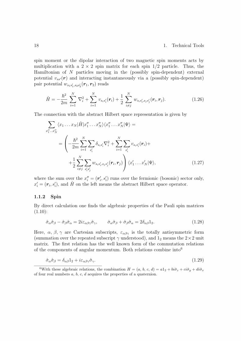
spin moment or the dipolar interaction of two magnetic spin moments acts bymultiplication with a 2 × 2 spin matrix for each spin 1/2 particle. Thus, theHamiltonian of N particles moving in the (possibly spin-dependent) externalpotential vss′(r) and interacting instantaneously via a (possibly spin-dependent)pair potential ws1s′1,s2s′2(r1, r2) reads

H = − ~2

2m

N∑

i=1

∇2i +

N∑

i=1

vsis′i(ri) +

1

2

N∑

i6=j

wsis′i,sjs′j(ri, rj). (1.26)

The connection with the abstract Hilbert space representation is given by∑

x′′1 ...x′′

N

〈x1 . . . xN |H|x′′1 . . . x′′N〉〈x′′1 . . . x′′N |Ψ〉 =

=

− ~2

2m

N∑

i=1

∑

s′i

δsis′i∇2i +

N∑

i=1

∑

s′i

vsis′i(ri)+

+1

2

N∑

i6=j

∑

s′is′j

wsis′i,sjs′j(ri, rj)

〈x′1 . . . x′N |Ψ〉, (1.27)

where the sum over the x′′i = (r′i, s′i) runs over the fermionic (bosonic) sector only,

x′i = (ri, s′i), and H on the left means the abstract Hilbert space operator.

1.1.2 Spin

By direct calculation one finds the algebraic properties of the Pauli spin matrices(1.10):

σασβ − σβσα = 2iεαβγσγ , σασβ + σβσα = 2δαβ12. (1.28)

Here, α, β, γ are Cartesian subscripts, εαβγ is the totally antisymmetric form(summation over the repeated subscript γ understood), and 12 means the 2×2 unitmatrix. The first relation has the well known form of the commutation relationsof the components of angular momentum. Both relations combine into6

σασβ = δαβ12 + iεαβγσγ. (1.29)

6With these algebraic relations, the combination H = (a, b, c, d) = a12 + biσz + ciσy + diσx

of four real numbers a, b, c, d acquires the properties of a quaternion.


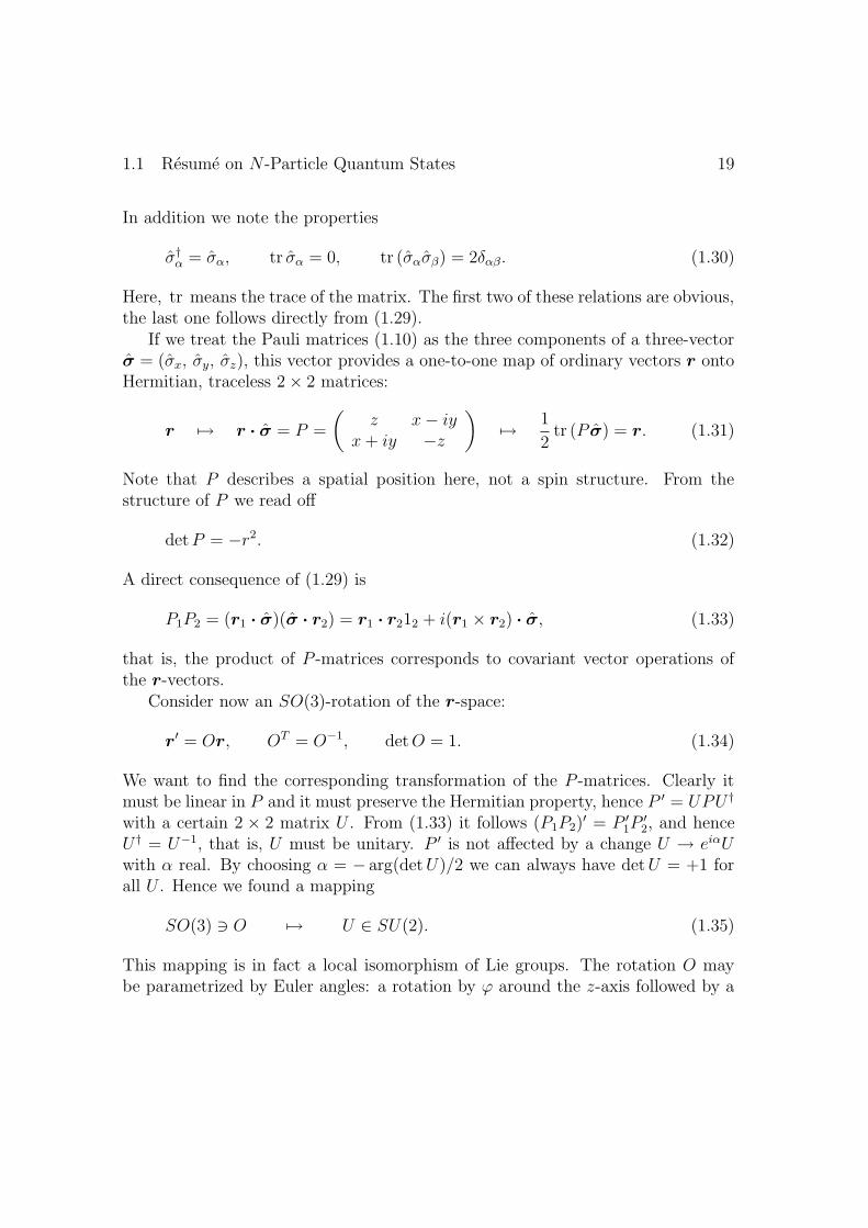
In addition we note the properties

σ†α = σα, tr σα = 0, tr (σασβ) = 2δαβ. (1.30)

Here, tr means the trace of the matrix. The first two of these relations are obvious,the last one follows directly from (1.29).

If we treat the Pauli matrices (1.10) as the three components of a three-vectorσ = (σx, σy, σz), this vector provides a one-to-one map of ordinary vectors r ontoHermitian, traceless 2 × 2 matrices:

r 7→ r · σ = P =

(

z x− iyx+ iy −z

)

7→ 1

2tr (P σ) = r. (1.31)

Note that P describes a spatial position here, not a spin structure. From thestructure of P we read off

detP = −r2. (1.32)

A direct consequence of (1.29) is

P1P2 = (r1 · σ)(σ · r2) = r1 · r212 + i(r1 × r2) · σ, (1.33)

that is, the product of P -matrices corresponds to covariant vector operations ofthe r-vectors.

Consider now an SO(3)-rotation of the r-space:

r′ = Or, OT = O−1, detO = 1. (1.34)

We want to find the corresponding transformation of the P -matrices. Clearly itmust be linear in P and it must preserve the Hermitian property, hence P ′ = UPU †

with a certain 2 × 2 matrix U . From (1.33) it follows (P1P2)′ = P ′1P

′2, and hence

U † = U−1, that is, U must be unitary. P ′ is not affected by a change U → eiαUwith α real. By choosing α = − arg(detU)/2 we can always have detU = +1 forall U . Hence we found a mapping

SO(3) 3 O 7→ U ∈ SU(2). (1.35)

This mapping is in fact a local isomorphism of Lie groups. The rotation O maybe parametrized by Euler angles: a rotation by ϕ around the z-axis followed by a


xx

XXXXXXXXXXXXy

z = z

CCCCCCCC

x′

y′

CCCCCCCCCCCC

¯z = z′

xϕ−→ x

θ−→ ¯xψ−→ x′

x

y = ¯y

¯x

PPqϕ

6ϕ

CCCCW

θ

-θ

:ψ

CCCCCO

ψ

Figure 1: Euler angles φ, θ, and ψ of an SO(3)-rotation

rotation by θ around the new y-axis followed by a rotation by ψ around the newz-axis (see Fig.1). The corresponding unitary transformation U is

U = ei2ψσze

i2θσye

i2ϕσz , (1.36)

where the exponentials are to be understood as power series:

ei2ϕσz = 1 + i

ϕ

2σz −

1

2!

(ϕ

2

)2

− i

3!

(ϕ

2

)3

σz + · · ·

=

(

cos(ϕ/2) + i sin(ϕ/2) 00 cos(ϕ/2) − i sin(ϕ/2)

)

, (1.37)


ei2θσy = 1 + i

θ

2σy −

1

2!

(

θ

2

)2

− i

3!

(

θ

2

)3

σy + · · ·

=

(

cos(θ/2) sin(θ/2)− sin(θ/2) cos(θ/2)

)

. (1.38)

Hence,

U =

(

cos(θ/2)ei(ψ+φ)/2 sin(θ/2)ei(ψ−φ)/2

− sin(θ/2)e−i(ψ−φ)/2 cos(θ/2)e−i(ψ+φ)/2

)

. (1.39)

With these formulas it is straightforwardly seen that, now applied to the spinoperator proper, for instance,

Oϕσ = (cosϕ σx − sinϕ σy, sinϕ σx + cosϕ σy, σz) = UϕσU†ϕ, (1.40)

where Oϕ is an SO(3) rotation by ϕ around the z-axis, acting on the componentsof the three-vector σ whose components are 2 × 2 spin matrices, while Uϕ is theSU(2) transformation (1.37), acting on a 2 × 2 spin matrix whose componentsare three-vectors. Analogous relations are straightforwardly obtained for the otherelementary Euler rotations and hence hold true for a general SO(3) rotation andits SU(2) counterpart (1.36).

Since r and σ are independent dynamical variables of an orbital, we mustdistinguish between the SO(3) rotation O of the position space as in (1.34) andthe SO(3) rotation O of the spin space as in (1.40). Since the latter can alwaysbe expressed through the SU(2) transformation U of (1.40), we will not use itany more, and in what follows, O means always a rotation of the r-space while arotation of the spin space is expressed by the corresponding transformation U .

If the Hamiltonian does not explicitly depend on the spin, then to every spinorsolution φ of the Schrodinger equation, φ′ = Uφ is again a solution, with the sameenergy in the stationary case. Analogously, if the potential is spherically symmetric,to every solution φ(r), φ′(r) = φ(O−1r) is again a solution. If, however, theHamiltonian contains a term proportional to l · σ where l is a vector of the positionspace (orbital angular momentum operator), that is, if spin-orbit coupling exists,then the only remaining symmetry transformations are simultaneous rotations ofposition and spin space by the same Euler angles:

φ′(rs) =∑

s′

Uss′φ(O−1rs′). (1.41)


In other words, spin-orbit coupling sets up a one-one correspondence betweendirections in position space and directions in spin space. The same is establishedby an interaction term proportional to B · σ, where B is an applied magnetic field(which is due to electric currents in position space). This means that a magneticspin moment is always based on this one-one correspondence between directions inposition and spin spaces. In the writings of the orbital transformations we haveused the notation of the transformation law of a tensor field (active transformationof the components and passive transformation of the function variable).

In the case of a many-particle state (1.18) one introduces a spin operator foreach particle so that the spin operator of the k-th particle acts according to

(k

σ Ψ)(. . . rksk . . .) =∑

s′k

σsks′

kΨ(. . . rks

′k . . .). (1.42)

((σα)ss′ is the matrix element of the Pauli matrix σα; in this notation, for fixed sand s′, σss′ = ((σx)ss′ , (σy)ss′ , (σz)ss′) is again a three-vector in spin space.) Thecommutation relations for those spin operators are obviously

k

σαl

σβ −l

σβk

σα= 2iδklεαβγk

σγ , (1.43)

since spin operators for different particles operate on different variables, they com-mute.

Since the spin operators for the Cartesian components of the spin do not com-mute, these components cannot be measured simultaneously. Nevertheless, in anystate (1.17) the expectation value of the vector spin is well defined according to

S =~

2〈φ|σ|φ〉 =

~

2

∑

ss′

∫

d3r φ∗(rs)σss′φ(rs′). (1.44)

The components of this vector fluctuate according to the general rule (1.3). Inthis respect there is a total analogy to the situation with an angular momentum.However, unlike the case of the angular momentum which is an intrinsicallynonlocal entity, there is even a local density of the vector spin expressed throughthe spin density matrix

nss′(r) = φ(rs)φ∗(rs′), (1.45)

the trace of which is the particle density:

n(r) = tr n(r) = n++(r) + n−−(r). (1.46)


If we define the vector spin density as

S(r) =~

2tr (n(r)σ) =

~

2

∑

ss′

ns′s(r)σss′ =~

2

∑

ss′

φ∗(rs)σss′φ(rs′), (1.47)

then (1.44) is obtained from (1.47) by integration over the r-space. Of course, theexistence of this vector spin density follows from the fact, that, unlike the orbitalmomentum operator, the spin operator commutes with the position operator (1.9).Moreover, the vector directions in this spin vector space are uniquely linked todirections of the position space in case of spin-orbit coupling or an applied magneticfield only.

For the N -particle state (1.18) the spin density matrix is defined as

nss′(r) = N

∫

dx2 · · · dxN Ψ(rs, x2 · · · xN)Ψ∗(rs′, x2 · · · xN). (1.48)

Since ΨΨ∗ is totally symmetric in the particle variables, a summation over allparticles can simply be replaced by N times the expression for particle 1. Hence,the connection with the total particle density and the total vector spin density orvector spin is the same as in (1.46), (1.47) and (1.44).

From (1.47) we read off the expressions for the Cartesian components of thevector spin density:

Sx(r) =~

2(n+−(r) + n−+(r)), Sy(r) = i

~

2(n+−(r) − n−+(r)),

Sz(r) =~

2(n++(r) − n−−(r)). (1.49)

The spin flip amplitudes for rising and lowering the z-component of the spin are

S+(r) = Sx(r) + iSy(r) = ~n−+(r),

S−(r) = Sx(r) − iSy(r) = ~n+−(r). (1.50)

(Check the relations σ+χ− = 2χ+, σ−χ

+ = 2χ− for σ± = σx ± iσy.) We havewritten down explicitly the r-dependence in all those expressions in order to makeclear that they are well defined densities.7

7To measure a density in (non-relativistic) quantum physics amounts to use the observable r,which is an idealized observable, in Schrodinger representation given by a δ-function multiplicationoperator. In truth, measuring a density means projection onto a well localized wave pocket.


1.1.3 Momentum Representation

Here, the main features of the momentum or plane wave representation used inthe following text are summarized.8 Formally it uses the eigenstates of the particlemomentum operator

p |k〉 = |k〉 ~k (1.51)

instead of the position vector eigenstates from (1.9) as basis vectors in the Hilbertspace of one-particle quantum states.

In Schrodinger representation, the particle momentum operator is given byp = (~/i)∇, and the momentum eigenstate (1.51) is represented by a wavefunction

φk(r) = 〈r|k〉 =1√Veik·r. (1.52)

V is the total volume or the normalization volume (often tacitly put equal to unity).In Solid State Theory it is convenient to use periodic boundary conditions also

called Born-von Karman boundary conditions. They avoid formal mathematicalproblems with little physical relevance with the continuous spectrum of energyeigenstates and simplify the treatment of the thermodynamic limes. They consistin replacing the infinite position space R3 of the particles by a large torus T 3 ofvolume V = L3 defined by

x+ L ≡ x, y + L ≡ y, z + L ≡ z, (1.53)

where (x, y, z) are the components of the position vector. The meaning of (1.53) isthat any function of x, y, z must fulfill the periodicity conditions f(x+ L) = f(x),and so on. As is immediately seen from (1.52), this restricts the spectrum ofeigenvalues k of (1.51) to the values

k =2π

L(nx, ny, nz) (1.54)

with integers nx, ny, nz. The k-values (1.54) form a simple cubic mesh in thewavenumber space (k-space) with a k-space density of states (number of k-vectors(1.54) within a unit volume of k-space)

D(k) =V

(2π)3, i.e.

∑

k

→ V

(2π)3

∫

d3k. (1.55)

8Pages 24 to 33 and 35 to 37 contain passages of text from [Eschrig, 2003] which is repeatedhere in order to make the present text sufficiently self-contained.


In the thermodynamic limes V → ∞ one simply has D(k)/V∑ · · · =

(2π)−3∑

s

∫

d3k · · · . Again we introduce a combined variable

qdef= (k, s),

∑

q

def=∑

s

∑

k

=V

(2π)3

∑

s

∫

d3k. (1.56)

for both momentum and spin of a particle.In analogy to (1.13), the N -particle quantum state is now represented by a

(spinor-)wavefunction in momentum space

Ψ(q1 . . . qN) = 〈 q1 . . . qN |Ψ〉 = 〈k1s1 . . .kNsN |Ψ〉 (1.57)

expressing the probability amplitude of a particle momentum (and possibly spin)configuration (q1 . . . qN) in complete analogy to (1.25). Everything that was saidin the preceding section between (1.9) and (1.25) transfers accordingly to thepresent representation. Particularly, in the case of fermions, Ψ of (1.57) is totallyantisymmetric with respect to permutations of the qi, and it is totally symmetricin the case of bosons. Its spin dependence is in complete analogy to that of theSchrodinger wavefunction (1.13).

Equation (1.4) reads in momentum representation

∑

(q′1...q′

N)

〈 q1 . . . qN |A| q′1 . . . q′N 〉〈 q′1 . . . q′N |Ψa〉 = 〈 q1 . . . qN |Ψa〉 a, (1.58)

where the summation runs over the physically distinguished states only.With this rule, it is a bit tedious but not really complicated to cast the

Hamiltonian (1.26) into the momentum representation:

〈 q1 . . . qN |H| q′1 . . . q′N 〉 =~

2

2m

∑

i

k2i

∏

j

δqjq′j+

+∑

i

vsıs′ikı−k′

i(∓1)P

∏

j(6=i)

δqq′j +

+1

2

∑

i6=j

[

wsıs′i,ss′jkı−k′

i,k−k′j∓ w

sıs′j ,ss′ikı−k′

j ,k−k′i

]

(∓1)P∏

k(6=i,j)

δqkq′k . (1.59)

Here, i = P ı, and P is a permutation of the subscripts which puts ı in theposition i (and puts in the position j in the last sum) and leaves the order of theremaining subscripts unchanged. There is always at most one permutation P (up


to an irrelevant interchange of ı and , and in the bosonic case up to ineffectivepermutations of identical states) for which the product of Kronecker δ’s can benon-zero. For the diagonal matrix element, that is q′i = qi for all i, P is the identityand can be omitted.

The Fourier transforms of vss′(r) and ws1s′1,s2s′2(r1, r2) are given by

vss′

k =1

V

∫

d3r vss′(r)e−ik·r (1.60)

and

ws1s′1,s2s

′2

k1,k2=

1

V 2

∫

d3r1 d3r2ws1s′1,s2s′2(r1, r2)e

−ik1·r1−ik2·r2 . (1.61)

The latter expression simplifies further, if the pair interaction depends on theparticle distance only.

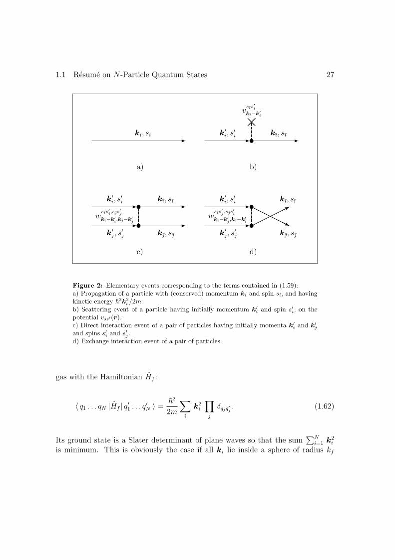
The elementary processes corresponding to the terms of (1.59) are depictedin Fig.2. The first sum of (1.59) is over the kinetic energies of the particlesin their momentum eigenstates (1.51, 1.52). Since the momentum operator ofsingle particles commutes with the kinetic energy operator of the system, thispart is diagonal in momentum representation, which is formally expressed by thej-product over Kronecker symbols δqjq′j . The next sum contains the individual

interaction events of particles with the external potential vss′(r). The amplitudeof this interaction process is given by the Fourier transform of the potential. Sincethe interaction of each particle with the external field is assumed to be independentof the other particles (the corresponding term of H is assumed to be a sum overindividual items vsls

′

l(rl) in (1.26)), all remaining particle states j 6= i are kept

unchanged in an interaction event in which one particle makes a transition fromthe state q′i to the state qı. The constancy of the remaining particle states is againexpressed by the j-product. Finally, the classical imagination of an elementaryevent of pair interaction is that particles in states k′is

′i and k′js

′j collide and are

scattered into states kısı and ks. Quantum-mechanically, one cannot decidewhich of the particles, formerly in states q′i, q

′j, is afterwards in the state qı and

which one is in the state q. This leads to the second term in (1.59), the exchangeterm with qı and q reversed. For a fermionic system, the exchange term appearswith a negative sign, and for a bosonic system, with a positive sign.

An important reference system is formed by interaction-free fermions (w = 0) ina constant external potential vss′(r) = 0: the homogeneous interaction-free fermion


-ki, si

a)

- -u

@@k′i, s

′i kı, sı

vsıs′ikı−k′

i

b)

- -

- -u

uk′i, s

′i

k′j, s′j

kı, sı

k, s

wsıs′i,ss′jkı−k′

i,k−k′j

c)

-

-

HHHHHHj*

u

uk′i, s

′i

k′j, s′j

kı, sı

k, s

wsıs′j ,ss′ikı−k′

j ,k−k′i

d)

Figure 2: Elementary events corresponding to the terms contained in (1.59):a) Propagation of a particle with (conserved) momentum ki and spin si, and havingkinetic energy ~

2k2i /2m.

b) Scattering event of a particle having initially momentum k′i and spin s′i, on the

potential vss′(r).c) Direct interaction event of a pair of particles having initially momenta k′

i and k′j

and spins s′i and s′j .d) Exchange interaction event of a pair of particles.

gas with the Hamiltonian Hf :

〈 q1 . . . qN |Hf | q′1 . . . q′N 〉 =~

2

2m

∑

i

k2i

∏

j

δqjq′j . (1.62)

Its ground state is a Slater determinant of plane waves so that the sum∑N

i=1 k2i

is minimum. This is obviously the case if all ki lie inside a sphere of radius kf


determined by

N =

ki≤kf∑

qi

1 = (2S + 1)V

(2π)3

∫

k≤kf

d3k, (1.63)

where the factor (2S + 1) in front of the last expression comes from summationover the spin values for each k. Hence

N

V= n = (2S + 1)

k3f

6π2(1.64)

with n denoting the constant particle density in position space of this ground state,related to the Fermi radius kf . The Fermi sphere of radius kf in k-space separatesthe occupied orbitals 〈r|k〉 from the unoccupied ones. The ground state energy is

E = (2S + 1)∑

k≤kf

~2k2

2m=

3~2k2f

10mN (1.65)

implying an average energy per particle

ε =E

N=

3~2k2f

10m(1.66)

in the ground state of the homogeneous interaction-free fermion gas.

1.1.4 Heisenberg Representation

The notations (1.27) and (1.58) specify the Schrodinger and momentumrepresentations to be special cases of a more general scheme.

Let |L〉 be any given complete orthonormal set of N -particle states labelledby some multi-index L. Any state may then be expanded according to

|Ψ〉 =∑

L

|L〉CL =∑

L

|L〉〈L|Ψ〉, (1.67)

and the eigenvalue equation (1.4) takes on the form of a matrix problem:

∑

L′

[ALL′ − aδLL′ ]CL′ = 0, ALL′ = 〈L|A|L′〉. (1.68)


with an infinite matrix ‖A‖ and the eigenstate with eigenvalue a represented by acolumn vector C. This is Heisenberg’s matrix mechanics.

To be a bit more specific, consider a fermion system and let φl(x) bea complete orthonormal set of single-particle (spin-)orbitals. Let ΦL, L =(l1 . . . lN) run over the N -particle Slater determinants (1.19) of all possible orbitalconfigurations (again using some linear order of the l-labels). In analogy to (1.59–1.61) one now gets

HLL′ =∑

i

⟨

lı

∣

∣

∣

∣

− ~2

2m∇2 + v

∣

∣

∣

∣

l′i

⟩

(−1)P∏

j(6=i)

δll′j +

+1

2

∑

i6=j

[

〈lıl|w|l′il′j〉 − 〈lıl|w|l′jl′i〉]

(−1)P∏

k(6=i,j)

δlkl′k (1.69)

for the Hamiltonian with i = P ı, and P is defined in the same way as in (1.59),particularly again P = identity for L′ = L. The orbital matrix elements are

〈l|h|m〉 def=

⟨

l

∣

∣

∣

∣

− ~2

2m∇2 + v

∣

∣

∣

∣

m

⟩

=

=∑

ss′

∫

d3r φ∗l (r, s)

[

− ~2

2m∇2δss′ + vss′(r)

]

φm(r, s′) (1.70)

and

〈lm|w|pq〉 =∑

s1s′1s2s′2

∫

d3r1d3r2 φ

∗l (r1, s1)φ

∗m(r2, s2) ∗

∗ws1s′1,s2s′2(r1, r2)φq(r2, s′2)φp(r1, s

′1). (1.71)

Clearly, 〈lm|w|pq〉 = 〈ml|w|qp〉.

1.1.5 Hartree-Fock Theory

For an interacting N -fermion system, a single Slater determinant (1.19) can ofcourse not be a solution of the stationary Schrodinger equation. However, onecan ask for the best Slater determinant approximating the true N -particle groundstate as that one which minimizes the expectation value of the Hamiltonian Hamong Slater determinants. The corresponding minimum value will estimate thetrue ground state energy from above.


This would, however, in general be a too restrictive search. The point isthat in most cases of interest the Hamiltonian H does not depend on the spinsof the particles: vss′(r) = δss′v(r) and ws1s′1,s2s′2(r1, r2) = δs1s′1δs2s′2w(|r1 −r2|). Consequently, the true ground state has a definite total spin S2 =〈∑x,y,z

α (∑

i σiα)2〉, whereas a Slater determinant of spin-orbitals in general does

not have a definite total spin; rather such a spin eigenstate can be build as a linearcombination of Slater determinants with the same spatial orbitals but differentsingle-particle spin states occupied. Depending on whether the total spin of theground state is zero or non-zero, the approach is called the closed-shell and open-shell Hartree-Fock method, respectively.

We restrict our considerations to the simpler case of closed shells of spin-halfparticles and will see in a minute that in this special case a determinant of spin-orbitals would do. In this case, the number N of spin-half particles must be evenbecause otherwise the total spin would again be half-integer and could not bezero. A spin-zero state of two spin-half particles is obtained as the antisymmetriccombination of a spin-up and a spin-down state:

〈s1s2|S = 0〉 =1√2

(

χ+(s1)χ−(s2) − χ−(s1)χ

+(s2))

. (1.72)

This is easily seen by successively operating with σ1α + σ2α, α = x, y, z (see (1.10,1.15)) on it, giving a zero result in all cases. Hence, a simple product of N/2 spinpairs in states (1.72) provides a normalized N -particle S = 0 spin state, which isantisymmetric with respect to particle exchange within the pair and symmetric withrespect to exchange of pairs. (It cannot in general be symmetric or antisymmetricwith respect to exchange between different pairs.)

The two particles in the spin state (1.72) may occupy the same spatial orbitalφ(r), maintaining the antisymmetric character of the pair wavefunction

Φ(x1x2) = φ(r1)φ(r2)〈s1s2|S = 0〉. (1.73)

If, for even N , we consider a Slater determinant of spin orbitals, where each spatialorbital is occupied twice with spin up and down, and expand the determinantinto a sum over permutations of products, then a permutation within a doublyoccupied orbital does not change the spatial part of those terms. For the spin part,all those permutations just combine to a product of N/2 spin-zero states (1.72).Now take any permuted product appearing in the expansion of the determinant. Ithas been either part of the just considered combination or not. If not, take againall permutations within pairs of equal spatial orbitals (which all have not been


part of the former combination) to get another product of N/2 spin-zero states.The total Slater determinant is thus a linear combination of products of spin-zerostates, hence it is itself a spin-zero state in this special case. Moreover, as a Slaterdeterminant it has the correct antisymmetry with respect to all particle exchangeoperations. Therefore, such a single Slater determinant can provide a spin-zeroapproximant to a closed-shell ground state.

Now, take (for even N) N/2 spatial orbitals φi and build a Slater determinantwith spin-orbitals φi+(xk) in the first N/2 rows and with spin-orbitals φi−(xk) inthe lower N/2 rows. Using the Laplace expansion, this Slater determinant may bewritten as

ΦHF(x1 . . . xN) =(N/2)!√N !

∑

k|k′

(−1)k|k′

(N/2)!det ‖φi+(xk)‖ det ‖φi−(xk′)‖,

(1.74)

where k|k′ means a selection of N/2 numbers k among the numbers 1,. . . ,N ,the remaining unselected numbers being denoted by k′. There are N !/(N/2)!2

different selections to be summed up with an appropriately chosen sign for eachitem. The items of the sum are normalized, and they are orthogonal to each otherwith respect to their spin dependence, because they differ in the selection of thevariables of spin-up particles. Hence there are no crossing matrix elements for anyspin independent operator, and its expectation value may be calculated just withone of the terms in the sum of (1.74), all terms giving the same result.

With the help of (1.69–1.71) the expectation value of the Hamiltonian (withs-independent external potential v) in the state (1.74) is easily obtained to be

EHF = 〈ΦHF|H|ΦHF〉 = 2

N/2∑

i=1

〈i|h|i〉 + 2

N/2∑

i,j=1

〈ij|w|ij〉 −N/2∑

i,j=1

〈ij|w|ji〉.

(1.75)

The three terms are called in turn one-particle energy, Hartree energy, and exchangeenergy. Summation over both spin directions for each orbital φi results in factors 2for the one-particle term, 4 for the Hartree term, but only 2 for the exchange termbecause the contained matrix element is only nonzero if both interacting particleshave the same spin direction. (Recall that the interaction part of the Hamiltoniancomes with a pre-factor 1/2.) Note that both the Hartree and exchange terms fori = j contain (seemingly erroneously) the self-interaction of a particle in the orbital


φi with itself. Actually those terms of the Hartree and exchange parts mutuallycancel in (1.75) thus not posing any problem.

In order to find the minimum of this type of expression one must vary theorbitals keeping them orthonormal. However, as we already know, the determinantremains unchanged upon an orthogonalization of the orbitals, and hence it sufficesto keep the orbitals normalized while varying them. Adding the normalizationintegral for φk, multiplied with a Lagrange multiplier 2εk, to (1.75) and then varyingφ∗k leads to the minimum condition

h φk(r) + vH(r)φk(r) + (vX φk)(r) = φk(r)εk (1.76)

with the Hartree potential

vH(r) = 2

N/2∑

j=1

∫

d3r′ φ∗j(r′)w(|r − r′|)φj(r′) (1.77)

and the exchange potential operator

(vX φk)(r) = −N/2∑

j=1

∫

d3r′ φ∗j(r′)w(|r − r′|)φk(r′)φj(r). (1.78)

(φ∗k is varied independently of φk which is equivalent to independently varyingthe real and imaginary parts of φk; the variation then is carried out by using thesimple rule δ/δφ∗k(x)

∫

dx′ φ∗k(x′)F (x′) = F (x) for any expression F (x) independent

of φ∗k(x).)The Hartree-Fock equations (1.76) have the form of effective single-particle

Schrodinger equations

F φk = φk εk, (1.79)

where the Fock operator F = −(~/2m)∇2 + veff consists of the kinetic energyoperator and an effective potential operator

veff = v + vH + vX (1.80)

called the mean field or molecular field operator.For a given set of N/2 occupied orbitals φi the Fock operator F as an integral

operator is the same for all orbitals. Hence, from (1.79), the Hartree-Fock orbitals

1.2 The Fock Space 33

may be obtained orthogonal to each other. From (1.76) it then follows that

N/2∑

i=1

εi =

N/2∑

i=1

〈i|h|i〉 + 2

N/2∑

i,j=1

〈ij|w|ij〉 −N/2∑

i,j=1

〈ij|w|ji〉. (1.81)

Comparison with (1.75) yields

EHF =

N/2∑

i=1

(εi + 〈i|h|i〉) = 2

N/2∑

i=1

εi − 〈W 〉 (1.82)

for the total Hartree-Fock energy. The sum over all occupied εi (including the spinsum) double-counts the interaction energy.

Coming back to the expression (1.75), one can ask for its change, if oneremoves one particle in the Hartree-Fock orbital φk (of one spin direction)while keeping all orbitals φj un-relaxed. This change is easily obtained to be

−〈k|h|k〉 − 2∑

j 〈kj|w|kj〉 +∑

j 〈kj|w|jk〉, which is just −εk as seen from (1.76–1.78). For a given set of occupied φi, (1.79) yields also unoccupied orbitals assolutions. The change of (1.75), if one additionally occupies one of those latterorbitals φk, is analogously found to be +εk. These results, which may be writtenas

(

∂EHF

∂nk

)

φj

= εk (1.83)

with nk denoting the occupation number of the Hartree-Fock orbital φk andthe subscript φj indicating the constancy of the orbitals, goes under the nameKoopmans’ theorem [Koopmans, 1934]. It guarantees in most cases that theminimum of EHF is obtained if one occupies the orbitals with the lowest εi, becauseremoving a particle from φi and occupying instead a state φj yields a change ofEHF equal to εj − εi plus the orbital relaxation energy, which is usually smallerthan εj − εi in closed shell situations.

1.2 The Fock Space

Up to here we considered representations of quantum mechanics with the particlenumber N of the system fixed. If this number is macroscopically large, it cannot befixed at a single definite number in experiment. Zero mass bosons as e.g. photons


may be emitted or absorbed in systems of any scale. (In a relativistic descriptionany particle may be created or annihilated, possibly together with its antiparticle,in a vacuum region just by applying energy.) From a mere technical point of view,quantum statistics of identical particles is much simpler to formulate with thegrand canonical ensemble with varying particle number, than with the canonicalone. Hence there are many good reasons to consider quantum dynamics withchanges in particle number.

In order to do so, we start with building the Hilbert space of quantum statesof this wider frame: the Fock space. The considered up to now Hilbert spaceof all N -particle states having the appropriate symmetry with respect to particleexchange will be denoted by HN . In Subsection 1.1.4 an orthonormal basis |L〉 of(anti-)symmetrized products of single-particle states out of a given fixed completeand ortho-normalized set φi of such single-particle states was introduced. Theset φi with some fixed linear order (φ1, φ2, . . .) of the orbitals will play a centralrole in the present section. The normalized states |L〉 will alternatively be denotedby

|n1 . . . ni . . .〉,∑

i

ni = N, (1.84)

where ni denotes the occupation number of the i-th single-particle orbital in thegiven state |L〉. For fermions, ni = 0, 1, for bosons ni = 0, 1, 2, . . .. Twostates (1.84) not coinciding in all occupation numbers ni are orthogonal. HN isthe complete linear space spanned by the basis vectors (1.84), i.e. the states ofHN are either linear combinations

∑ |L〉CL of states (1.84) (with the sum of thesquared absolute values of the coefficients CL equal to unity) or limits of Cauchysequences of such linear combinations. A Cauchy sequence is a sequence |Ψn〉with limm,n→∞ 〈Ψm−Ψn|Ψm−Ψn〉 = 0. The inclusion of all limits of such sequencesinto HN means realizing the topological completeness property of the Hilbert space,being extremely important in all considerations of limits. This completeness ofthe space is not to be confused with the completeness of a basis set φi. Theextended Hilbert space F (Fock space) of all states with the particle number Nnot fixed is now defined as the completed direct sum of all HN . It is spanned byall state vectors (1.84) for all N with the above given definition of orthogonalityretained, and is completed by corresponding Cauchy sequences, just as the realline is obtained from the rational line by completing it with the help of Cauchysequences of rational numbers. (A mathematical rigorous treatment can be found,e.g. in [Cook, 1953, Berezin, 1965].)


Note that F now contains not only quantum states which are linearcombinations with varying ni so that ni does not have a definite value in thequantum state (occupation number fluctuations), but also linear combinationswith varying N so that now quantum fluctuations of the total particle numberare allowed too. For bosonic fields (as e.g. laser light) those quantum fluctuationscan become important experimentally even for macroscopic N .

1.2.1 Occupation Number Representation

In order to introduce the possibility of a dynamical change of N , operators mustbe introduced providing such a change. For bosons those operators are introducedas

bi| . . . ni . . .〉 = | . . . ni − 1 . . .〉√ni, (1.85)

b†i | . . . ni . . .〉 = | . . . ni + 1 . . .〉√ni + 1. (1.86)

These operators annihilate and create, respectively, a particle in the orbital φi andmultiply by a factor chosen for the sake of convenience. Particularly, in (1.85) itprevents producing states with negative occupation numbers. (Recall that the niare integers; application of bi to a state with ni = 0 gives zero instead of a statewith ni = −1.) Considering all possible matrix elements with the basis states(1.84) of F , one easily proves that b and b† are Hermitian conjugate to each other.In the same way the key relations

ni| . . . ni . . .〉 def= b†i bi| . . . ni . . .〉 = | . . . ni . . .〉ni, (1.87)

and

[bi, b†j] = δij, [bi, bj] = 0 = [b†i , b

†j] (1.88)

are proven, where the brackets in standard manner denote the commutator

[bi, b†j]

def= [bi, b

†j]− = bib

†j − b†j bi. The occupation number operator ni is Hermitian

and can be used to define the particle number operator

N =∑

i

ni (1.89)

having arbitrarily large but always finite expectation values in the basis states(1.84) of the Fock space F . The Fock space itself is the complete hull (in the above


described sense) of the linear space spanned by all possible states obtained fromthe normalized vacuum state

|〉 def= |0 . . . 0 . . .〉, bi|〉 = 0 for all i (1.90)

by applying polynomials of the b†i to it. This situation is expressed by saying that

the vacuum state is a cyclic vector of F with respect to the algebra of the bi andb†i . Obviously, any operator in F , that is any operation transforming vectors of Flinearly into new ones, can be expressed as a power series of operators b†i and bi.This all together means that the Fock space provides an irreducible representationspace for the algebra of operators b†i and bi, defined by (1.88).

For fermions, the definition of creation and annihilation operators must haveregard for the antisymmetry of the quantum states and for Pauli’s exclusionprinciple following from this antisymmetry. They are defined by

ci| . . . ni . . .〉 = | . . . ni − 1 . . .〉ni (−1)P

j<i nj , (1.91)

c†i | . . . ni . . .〉 = | . . . ni + 1 . . .〉 (1 − ni) (−1)P

j<i nj . (1.92)

Again by considering the matrix elements with all possible occupation numbereigenstates (1.84), it is easily seen that these operators have all the neededproperties, do particularly not create non-fermionic states (that is, states withoccupation numbers ni different from 0 or 1 do not appear: application of ci to astate with ni = 0 gives zero, and application of c†i to a state with ni = 1 gives zeroas well). The ci and c†i are mutually Hermitian conjugate, obey the key relations

ni| . . . ni . . .〉 def= c†i ci| . . . ni . . .〉 = | . . . ni . . .〉ni (1.93)

and

[ci, c†j]+ = δij, [ci, cj]+ = 0 = [c†i , c

†j]+ (1.94)

with the anti-commutator [ci, c†j]+ = cic

†j + c†j ci defined in standard way. Their role

in the fermionic Fock space F is completely analogous to the bosonic case. (The c†-and c-operators of the fermionic case form a normed complete algebra provided witha norm-conserving adjoint operation †, called a c∗-algebra in mathematics. Sucha (normed) c∗-algebra can be formed out of the bosonic operators b† and b, whichthemselves are not bounded in F , by complex exponentiation. For a comprehensivetreatment on the level of mathematical physics see [Bratteli and Robinson, 1987].)


As an example, the Hamiltonian (1.69) is expressed in terms of creation andannihilation operators and orbital matrix elements (1.70, 1.71) as

H =∑

ij

c†i〈i|h|j〉cj +1

2

∑

ijkl

c†i c†j〈ij|w|kl〉clck (1.95)

Observe the order of operators being important in expressions of that type; thisHamiltonian is indeed equivalent to (1.69) for every N since it does not change thetotal particle number. The present form is easily verified by considering the matrixelement 〈L|H|L′〉 with |L〉 and |L′〉 represented in notation (1.84), and comparingthe result with (1.69).

Generally, an operator is said to be in normal order, if it is arranged in eachterm so that all creators are left of all annihilators. The result of normal-orderingan operator A is indicated by colons, : A :. It is obtained by just (anti)commutingthe factors in all terms of A. By applying the (anti)commutation rules for theb- and c-operators, every operator can be identically transformed into a sum ofnormal-ordered operators. For instance, : bb† : = b†b, but bb† = b†b+1 = : bb† : +1.The merit of normal order is that vacuum expectation values vanish for all termscontaining at least one creation or annihilation operator.

In order to write down some useful relations holding accordingly in both thebosonic and fermionic cases, we use operator notations ai and a†i denoting either abosonic or a fermionic operator. One easily obtains

[ni, ai] = −ai, [ni, a†i ] = a†i (1.96)

with the commutator in both the bosonic and fermionic cases.Sometimes it is useful (or simply hard to be avoided) to use a non-orthogonal

basis φi of single-particle orbitals. The whole apparatus may be generalized tothis case by merely generalizing the first relations (1.88) and (1.94) to

[ai, a†j]± = 〈φi|φj〉, (1.97)

which generalization of course comprises the previous relations of the orthogonalcases. Even with a non-orthogonal basis φi the form of the original relations(1.88) and (1.94) may be retained, if one defines the operators ai with respect tothe φi and replaces the operators a†i by modified creation operators a+

i with respectto a contragredient basis χi, 〈φi|χj〉 = δij. Of course, this way the a+

i are nolonger Hermitian conjugate to the ai.


1.2.2 Coherent Bosonic States

The states (1.84) are simultaneously eigenstates of all occupation number operatorsni = a†i ai, ai = bi or ai = ci, as seen from (1.87) and (1.93). Most of those statesare not eigenstates of the creation or annihilation operators as is likewise seen from(1.85, 1.86) and (1.91, 1.92). It is easily verified that a bosonic creator b†i hasno ordinary eigenstate at all in the Fock space. (Exercise. Take a general state∑ |L〉CL and let NL be the total particle number in the component |L〉. Let NL0

be the minimum number NL for which CL is non-zero. It exists since NL ≥ 0 andNL <∞. Apply b†i .)

Remarkably enough, besides the vacuum there exist simultaneous eigenstatesof all bosonic annihilators bi (the bi commute with one another) in the Fock space[Glauber, 1963]. For reasons which become clear at the end of this subsection, theyare called coherent states.

Consider the eigenvalue equations (for all i simultaneously)

bi |b〉 = |b〉 bi (1.98)

and use the occupation number notation

|b〉 =∑

|n1 . . . ni . . .〉Cn1...ni.... (1.99)

From (1.85) it follows by projection onto one basis state that

Cn1...ni...

√ni = Cn1...ni−1...bi. (1.100)

The state |n1 . . . ni . . .〉 can be created out of the vacuum state (1.90) as

|n1 . . . ni . . .〉 =(b†1)

n1

√n1!

· · · (b†i )ni

√ni!

· · · |〉. (1.101)

(Induction of (1.86).) The last two relations yield, again by induction,

|b〉 =∑

n1...ni...

(b1b†1)n1

n1!· · · (bib

†i )ni

ni!· · · |〉 =

= exp(

∑

bib†i

)

|〉. (1.102)

Here and in the following, the sum in the exponent runs over the subscript, i inthe present case. The bi may be arbitrary complex numbers.


Hermitian conjugation of equations (1.98) and (1.102) yields

〈b| b†i = b∗i 〈b| (1.103)

wherefore 〈b| is called a left eigenstate of the b†i , and

〈b| = 〈| exp(

∑

bib∗i

)

. (1.104)

Hence,

〈b|b′〉 = 〈| exp(

∑

bib∗i

)

exp(

∑

b′j b†j

)

|〉 = exp(

∑

b∗i b′i

)

. (1.105)

After rewriting the two exponentials of sums into products of exponentials andexpanding the latter into series, the nonzero vacuum expectation values are thosecontaining factors bi and b†i in pairs only. Considering (1.88) yields the final result(exercise).

We conclude that (generally non-normalized) coherent states are all states(1.102), for which

∑ |bi|2 is finite, the complex numbers bi may otherwise be

completely arbitrary. This may be expressed by saying that the annihilators bihave a complex continuous spectrum. Moreover, by expanding the exponential in(1.102) we find

〈|b〉 = 1 (1.106)

for all |b〉.Applying a creator to a (right) coherent state (1.102) yields

b†i |b〉 = b†i exp(

∑

bj b†j

)

|〉 =∂

∂biexp

(

∑

bj b†j

)

|〉 =∂

∂bi|b〉 (1.107)

and likewise, from (1.104),

〈b| bi =∂

∂b∗i〈b|. (1.108)

This can be used to evaluate the following commutator:[

bi ,

∫

∏

j

d2bjπ

|b〉 exp(

−∑

b∗kbk

)

〈b|]

=

=

∫

∏

j

d2bjπ

|b〉 exp(

−∑

b∗kbk

)

(

bi −∂

∂b∗i

)

〈b|

= 0. (1.109)


The measure d2z = dxdy, z = x + iy was introduced in the complex plane. Inthe second line, (1.98) and (1.108) was used. Instead of using the independentvariables Re bj, Im bj in the complex bj-plane, b∗j and bj may likewise be consideredindependent, with dRe bjdIm bj = ∂(Re bj, Im bj)/∂(b∗j , bj) db

∗jdbj = db∗jdbj/2i,

hence d2bj/π = db∗jdbj/(2πi). Then, |b〉 depends on bj, that is, on the combinationRe bj + iIm bj only, and 〈b| depends on b∗j only. An integration by parts gives azero result in (1.109). The Hermitian conjugate of this result is

[

∫

∏

j

d2bjπ

|b〉 exp(

−∑

b∗kbk

)

〈b| , b†i

]

= 0. (1.110)

Now, recall that the Fock space is an irreducible representation space of the algebraof the bi and the b†i . That implies, that an operator commuting with all bi and all

b†i must be proportional to the unit operator (Schur’s lemma). Hence the abovemulti-integral must be a c-number. Its value may be obtained by taking the vacuumexpectation value. Considering (1.106) one finds that

∫

∏

j

d2bjπ

|b〉 exp(

−∑

b∗kbk

)

〈b| = 1 (1.111)

is the coherent state representation of the unit operator in the bosonic Fock space.Note, however, that the coherent states |b〉 are not orthogonal to each other asexplicitly seen from (1.105, 1.106).

In analogy to (1.67, 1.68), a coherent state representation for every quantumstate |Ψ〉 and for every operator A in the Fock space may be introduced. With thehelp of the unit operator (1.111),

|Ψ〉 =

∫

∏ d2biπ

|b〉 exp(

−∑

b∗kbk

)

Ψ(b∗), Ψ(b∗)def= 〈b|Ψ〉. (1.112)

Here, Ψ(b∗) = Ψ(b∗1 . . . b∗i . . .) figures as a ‘wavefunction’, compare to |Ψ〉 =

∫

d3r |r〉〈r|Ψ〉. In analogy to (1.27) we find from (1.108, 1.103)

〈b|bi|Ψ〉 =∂

∂b∗iΨ(b∗), 〈b|b†i |Ψ〉 = b∗i Ψ(b∗). (1.113)

This yields the annihilation and creation operators

bi =∂

∂b∗i, b†i = b∗i (1.114)


in coherent state representation. For instance, the Schrodinger equation with theHamiltonian (1.95) reads in coherent state representation

(

∑

ij

b∗i 〈i|h|j〉∂

∂b∗j+

1

2

∑

ijkl

b∗i b∗j〈ij|w|kl〉

∂

∂b∗k

∂

∂b∗l

)

Ψ(b∗) = Ψ(b∗)E. (1.115)

The matrix elements are the same as in (1.70, 1.71).On the other hand, for the matrix elements of a normal-ordered Fock space

operator : A(b†i , bj) : with coherent states one simply finds (exercise)

〈b| : A(b†i , bj) : |b′〉 = A(b∗i , b′j) exp

(

∑

b∗kb′k

)

, (1.116)

where A(b∗i , b′j) means that in the algebraic expression of A(b†i , bj) each entry of b†i

is replaced with the complex number b∗i and each entry of bj with b′j. For instance,in a coherent state,

〈ni〉 =〈b|b†i bi|b〉〈b|b〉 = |bi|2 (1.117)

and

∆ni〈ni〉

= 〈ni〉−1/2. (1.118)

(Exercise. Transformation to normal order of n2i is the essential issue.) In a

coherent state, the relative particle number fluctuations vanish for macroscopicmode occupation.

Consider a single one-dimensional harmonic oscillator with Hamiltonian

H = b†~ωb, b† =1√2~ω

(ωx− ip), b =1√2~ω

(ωx+ ip). (1.119)

(The mass is put to unity.) For the Schrodinger wavefunction ψb(x) = 〈x|b〉 wehave

〈x|b〉 b = 〈x|b|b〉 =〈x|ωx+ ip|b〉√

2~ω=

1√2~ω

(

ωx+ ~∂

∂x

)

〈x|b〉, (1.120)

i.e.,

∂

∂xψb(x) =

(

√

2ω

~b− ω

~x

)

ψb(x) (1.121)


with the solution

ψb(x) = C(b) exp

(

−[√

ω

2~x− b

]2)

. (1.122)

C is the integration constant which in general may of course depend on b. This isa minimum uncertainty wave pocket with its center of gravity at x =

√

2~/ωRe b.(For b = 0, i.e. the Fock space vacuum, it is just the oscillator ground state; itis normalized to unity with C(0) = (ω/π~)1/4. The normalization (1.106) means∫

dxψ∗0(x)ψb(x) = 1, yielding C(b) = C(0) exp(b2/2).) Now, in the Heisenberg

picture b → b exp(−iωt) and hence, in (1.120), b → b exp(−iωt): the center ofgravity of the wave pocket oscillates with the classical oscillator frequency andan arbitrary amplitude determined by b. The phases of the oscillator quanta arecoherently related in such a way that the wave pocket moves in the minimumuncertainty shape without decaying. The situation can directly be transferred tophotons, where coherent states describe traveling minimum uncertainty light pulseswith arbitrary amplitudes. It is this context in which coherent states providea limiting transition from bosonic quantum states to well localized particle-likeclassical wave pockets.

1.2.3 Grassmann Numbers

In the fermion case, the only eigenvalue for both creators c†i and annihilators ci inthe physical Hilbert space is zero since from (1.94) c†2i = 0 = c2i . It is, however,useful to introduce a formal symmetry between bosons and fermions, which hasgot the name super-symmetry in physical theories, but which is not realized in ourworld (it is speculated that it could have been spontaneously broken in the world’spresent state). To this goal, since non-zero complex numbers cannot be eigenvaluesof fermionic annihilators, abstract super-number generators ζi are introduced, whichanti-commute

ζiζj + ζjζi = 0, i.e. ζ2i = 0 (1.123)

and hence generate a Grassmann algebra, whence the name Grassmann numbers.(To contrast anti-commuting numbers with commuting numbers, the names a-number and c-number, respectively, are often used; a product of two a-numbersis a c-number.) A super-analysis is developed for super-numbers (as well as asuper-algebra, super-topology, . . . ).


A general super-number is a general holomorphic function (power series) of thesuper-number generators

f(ζi) = z0 +∑

i

ziζi +∑

i6=j

zijζiζj + · · · , (1.124)

where the z are complex coefficients commuting with every super-number, and eachterm of the series cannot contain higher then first powers of each variable ζi due tothe second relation (1.123). The complex number fb = z0 is said to be the ‘body’of f , and the remainder fs = f − fb its ‘soul’. The soul consists of an a-numberpart formed by the odd-order terms and a c-number part formed by the even-orderterms. Only an f with non-zero body has an inverse obtained as the power seriesof (fb + fs)

−1 in powers of fs. For instance the exponential function is

exp ζ = 1 + ζ. (1.125)

Thus, with respect to the ζi only derivatives of multi-linear functions are needed,and the only peculiarity here is that derivative operators with respect to super-number generators anti-commute with a-numbers and with each other:

∂

∂ζjζiζj = −ζi

∂

∂ζjζj = −ζi,

∂

∂ζi

∂

∂ζj= − ∂

∂ζj

∂

∂ζi. (1.126)

Integration∫

dζi f(ζj) is defined by the rules that dζi is again an anti-commutingsymbol, an integral of a complex linear combination is equal to the complex linearcombination of integrals, the result of integration over dζi does no longer dependon ζi, and, in order to enable integration by parts, the integral over a derivative iszero. These rules imply

∫

dζ z = 0,

∫

dζ zζ = z. (1.127)

The first result follows since z is the derivative of f(ζ) = zζ, and a constantc-number-factor left open by the above rules in the second result is defined byconvention (not uniquely in the literature).

Finally, a conjugation ζi → ζ∗i is introduced which groups the super-numbergenerators into pairs (where ζ∗i is different from ζi, so that ζ∗i ζi is non-zero9) and

9Caution, this is a special choice. In super-mathematics the generators of the super-algebra(distinctively denoted θk here) usually are defined to be ‘real’: θ∗k = θk. Our choice can then berealized by putting ζk = (θ2k−1 + iθ2k)/

√2, ζ∗k = (θ2k−1 − iθ2k)/

√2.


which obeys the rules

(zζ)∗ = z∗ζ∗, (ζiζj)∗ = ζ∗j ζ

∗i . (1.128)

Observe that conjugate Grassmann number generators just anti-commute asconjugate complex numbers just commute, in contrast to conjugate operators (1.94)and (1.88). A comprehensive introduction into super-mathematics accessible forphysicists is given in [DeWitt, 1992].

1.2.4 Coherent Fermionic States

Since coherent fermionic states do not exist in the physical Fock space F , this spacefirst must be generalized: the physical Fock space of fermions is generated by theoperators c†i . We attach to each operator ci a Grassmann number generator ζi andspecify anti-commutation between Grassmann number generators and c-operatorsas well as Hermitian conjugation to comprise Grassmann number conjugation inreversed order of all factors in a product, which also means the order of c-operatorsand Grassmann numbers to be reversed in a product. This way a Grassmannalgebra is specified and related to the algebra of fermion creators and annihilators.The generalized Fock space G is now defined as consisting of all linear combinationsof vectors of F with coefficients out of that Grassmann algebra (i.e. of the form(1.124)). The vectors of F have c-number properties as previously. The generalvectors of G inherit their commutation properties from the coefficients of theirexpansion into F -vectors.

In analogy to (1.102), except for a fermionic minus sign in the exponent, weconsider the state

|ζ〉 = exp(

−∑

ζic†i

)

|〉 =∏

(1 − ζic†i ) |〉. (1.129)

Since bilinear terms of anti-commuting quantities commute, the exponential ofa sum may simply be written as the product of individual exponentials, whichaccording to (1.125) reduce to linear expressions. Operation with an annihilator


on this state yields

ci |ζ〉 = ci∏

(1 − ζj c†j) |〉; =

=

∏

j(6=i)

(1 − ζj c†j)

(ci + ζicic†i ) |〉 =

=

∏

j(6=i)

(1 − ζj c†j)

ζi |〉 =

=

∏

j(6=i)

(1 − ζj c†j)

(1 − ζic†i ) |〉 ζi =

= |ζ〉 ζi. (1.130)

In the second line, ci was anti-commuted with ζi (while it commutes with all bilinearζj c†j for j 6= i). This step was anticipated by introducing the fermionic minus sign

in the exponent of (1.129). Then, in the third line, ci |〉 = 0 and cic†i |〉 = |〉 was

used. In the fourth line, a ‘nutritious’ zero was added (observe that ζi · · · ζi is zeroaccording to the Grassmann rules), whereupon it is seen, that |ζ〉 is a fermioniccoherent state, i.e., an eigenstate of all annihilators ci with Grassmann eigenvaluesζi.

Along similar lines one finds

〈ζ| c†i = ζ∗i 〈ζ|, 〈ζ| = 〈| exp(

−∑

ciζ∗i

)

(1.131)

and

〈ζ|ζ ′〉 = exp(

∑

ζ∗i ζ′i

)

, 〈|ζ〉 = 1 for all |ζ〉. (1.132)

(Exercise.)A physical fermion state is generated by applying creators to the vacuum:

|n1 . . . ni . . .〉 = (c†1)n1 · · · (c†i )ni · · · |〉. In view of the eigenvalue equation (1.130)

its overlap with a coherent state is

〈n1 . . . ni . . . |ζ〉 = 〈| · · · (ci)ni · · · (c1)n1 |ζ〉 = · · · ζni

i · · · ζn11 . (1.133)

Likewise, the matrix element of a normal-ordered Fock space operator : A(c†i , cj) :with coherent states is

〈ζ| : A(c†i , cj) : |ζ ′〉 = : A(ζ∗i , ζ′j) : exp

(

∑

ζ∗kζ′k

)

, (1.134)


where the right hand side has a meaning as in (1.116), except that now the orderof factors remains essential.

Observing the rules of the last subsection, (1.133) can be used to prove that

∫

∏

j

dζ∗j dζj |ζ〉 exp(

−∑

ζ∗kζk

)

〈ζ| = 1 (1.135)

is the unit operator in the physical Fock space F generated by the states (1.84) forall N (exercise).

Hence, although fermionic coherent states are unphysical (except for thevacuum), every physical fermionic state can be expanded into coherent states withthe help of (1.135):

|Ψ〉 =

∫

∏

dζ∗i dζi |ζ〉 exp(

−∑

ζ∗kζk

)

Ψ(ζ∗), Ψ(ζ∗)def= 〈ζ|Ψ〉. (1.136)

Again, Ψ(ζ∗) = Ψ(ζ∗1 . . . ζ∗i . . .) figures as a ‘wavefunction’ (observe the order of

arguments).

From (1 − ciζ∗i )ci = ci = (∂/∂ζ∗i )(1 − ciζ

∗i ) (since c2i = 0, and before applying

the derivative it must be anti-commuted with ci) as well as a conjugated relationone verifies

〈ζ| ci =∂

∂ζ∗i〈ζ|, c†i |ζ〉 = |ζ〉

←

∂

∂ζi. (1.137)

Again,

ci =∂

∂ζ∗i, c†i = ζ∗i (1.138)

is the coherent state representation of annihilation and creation operators.

If we finally declare a measure dµc of the coherent configuration space to be

dµcdef=∏

i

d2biπ

for bosons , dµcdef=∏

i

dζ∗i dζi for fermions (1.139)

and occasionally introduce a statistics sign factor η = ±1, we obtain a complete

1.3 Field Quantization 47

super-symmetry10 in the description of bosons and fermions within the coherentstate space G. Recall, however, that our real world does not show this (broken?)super-symmetry: it travels all the time through the subspace F of G only. While thesubspace F , the Fock space, contains all bosonic coherent states which quantum-mechanically describe real macroscopic fields as e.g. classical electromagnetic fields,it does not contain fermionic coherent states except of the vacuum, there are nomacroscopic fermionic fields in nature (not any more?).

For applications of supersymmetry in quantum theory of non-interactingparticles in a random potential see [Efetov, 1997].

1.3 Field Quantization

Quantum fields are obtained either by canonical quantization of classical fieldsvia canonical field variables defined with the help of a Lagrange density, or bycombining the Schrodinger orbitals and the corresponding creators and annihilatorsin Fock space. The latter route is often misleadingly called second quantizationalthough there is always only one quantization.

A spatial representation may be introduced in the Fock space by defining fieldoperators

ψ(x) =∑

i

φi(x)ai, ψ†(x) =∑

i

φ∗i (x)a†i , (1.140)

which obey the relations

[ψ(x), ψ†(x′)]± = δ(x− x′),

[ψ(x), ψ(x′)]± = 0 = [ψ†(x), ψ†(x′)]±. (1.141)

and provide a spatial particle density operator

n(x) = ψ†(x)ψ(x) (1.142)

10Formally this symmetry can be made even more explicit by using the generators θk of thefootnote on page 43, observing (dθk)2 = 0, and defining

∫

dθ zθ =√iπz at variance with (1.127).

This would imply

dµcdef=∏

k

dθ2kdθ2k−1

πfor fermions.

Since we are not really going to use super-symmetry we did not burden our analysis with formalfactors here.


having the properties

〈n(x)〉 =∑

ij

φ∗i (x)〈a†i aj〉φj(x),∫

dx n(x) =∑

i

a†i ai. (1.143)

These relations are readily obtained from those of the creation and annihilationoperators, and by taking into account the completeness and ortho-normality

∑

i

φi(x)φ∗i (x′) = δ(x− x′),

∫

dxφ∗i (x)φj(x) = δij (1.144)

of the basis orbitals.We may introduce a spin density matrix operator

nss′(r) = ψ†(rs′)ψ(rs) (1.145)

in accordance with (1.45) (which is its expectation value), and a vector spin densityoperator

S(r) =~

2tr n(r)σ (1.146)

in accordance with (1.47). Particularly, the spin flip operators are

S+(r) = ~ψ†(r+)ψ(r−), S−(r) = ~ψ†(r−)ψ(r+). (1.147)

They rise and lower the z-component of the spin by one quantum.In terms of field operators, the Hamiltonian (1.26) reads

H =

∫

dx ψ†(x)∑

s′

[

−~2

2δss′∇2 + vss′(r)

]

ψ(x′)+

+1

2

∫

dx1dx2 ψ†(x1)ψ

†(x2)∑

s′1s′2

ws1s′1,s2s′2(r1, r2) ψ(x′2)ψ(x′1), (1.148)

which is easily obtained by combining (1.95) with (1.140) and considering (1.75,1.76). As in (1.27), we use the notation x′ = (r, s′).

Field-quantized interaction terms contain higher-order than quadraticexpressions in the field operators and hence yield operator forms of equations ofmotion (in Heisenberg picture) which are nonlinear. Note, however, that, contraryto the Fock operator of (1.76), the Hamiltonians (1.95, 1.148) are linear operatorsin the Fock space of states |Ψ〉 as demanded by the superposition principle ofquantum theory. In this respect, the Fock operator rather compares to thoseoperator equations of motion than to a Hamiltonian.


1.3.1 Locality

As seen from (1.140), quantum field operators—or in short, quantum fields—arespatial densities of annihilators or creators. Hence, they are operators potentiallymaking up or changing fields in space rather then directly representing physicalfields being present in the laboratory. The latter appear as properties of quantumstates on which quantum field operators may act.

As potential fields, quantum fields must be defined in the whole infinite space-time. However, any actual manipulation on a physical system—which in quantumphysics is spoken of as a measuring process—takes place in a finite domain ofspace (and time). Hence, observables must be local constructs of quantum fields.For instance, a local orbital φk(x) is annihilated by

∫

dxφ∗k(x)ψ(x) = ak, which

immediately follows from the definition (1.140) of ψ(x) and the ortho-normality ofthe orbital set φk. Even this local annihilator is generally not yet an observable,because the process must be accompanied by something else, e.g. taking over theenergy and the spin of the annihilated state.

Consider arbitrarily often differentiable functions f, g, . . . vanishing outside ofa bounded closed domain of r-space. Define

ψ(f)def=

∫

dx f ∗(x)ψ(x), ψ†(g)def=

∫

dx ψ†(x)g(x). (1.149)

From (1.141),

[ψ(f), ψ†(g)]± =

∫

dxdx′ f ∗(x)[ψ(x), ψ†(x′)]±g(x′) =

=

∫

dx f ∗(x)g(x) =

def= (f |g) (1.150)

follows, and

[ψ(f), ψ(g)]± = 0 = [ψ†(f), ψ†(g)]±. (1.151)

The differentiability of the functions f, g, . . . together with their decay for large|r| ensures that independently of (1.140) derivatives of quantum fields canbe given a definite meaning through integration by parts of expressions like(1.149). Mathematically this means that quantum fields are operator-valueddistributions. This gives differential equations of motion for quantum fields adefinite mathematical content.


If the domains of f and g are spatially separated, corresponding manipulationson the system should be independent of each other, which means that thecorresponding observables should commute. (In relativistic theory this refers to thecase that one domain is outside of the light cone of the other.) This correspondsto (f |g) = 0 in that case. However, since fermion fields anticommute, observablesmust necessarily be composed of products of even numbers of fermion fields.

As we see, quantum fields by themselves are generally not observable.Observables are local constructs of quantum fields containing only products ofeven numbers of fermion fields.

1.3.2 Superselection

In Subsection 1.2.1 the algebra of creators c†i and annihilators ci was linked to theFock space in such a way, that the latter is an irreducible representation spaceof the former algebra. If there is a finite number of generators of the algebra(finite set of subscripts i), then it can be shown that all non-trivial irreduciblerepresentations11 are unitarily equivalent to this Fock space representation. (Everymatrix representation (c†i )LL′ , (ci)LL′ with respect to any complete orthogonalset |L〉—not necessarily linked to single-particle orbital occupations—can beunitarily transformed into (1.85, 1.86) or (1.91, 1.92), respectively.)

Consider as a related example the Pauli matrices (1.10). They have the algebraicproperties (1.29) reducing every product of Pauli matrices to a linear combination of12 and the σγ . Hence, the whole algebra generated by the Pauli matrices consistsof these linear combinations only. One may take (1.29), with 12 replaced by aunity of yet unknown dimension, as the defining relations for Pauli matrices andask for all possible non-trivial irreducible representations. These algebraic relationsare equivalent to (1.28) and hence contain the angular momentum commutationrelations (in units of ~/2) and the relations σ2

α = 1. Thus, σz may only haveeigenvalues ±1, and the only irreducible representations are two-dimensional.12

Every non-trivial irreducible representation σ ′α of (1.29) has the form σ′α = T σαT−1,

where σα are the ordinary Pauli matrices (1.10), and T is any regular complex 2×2matrix. (It must be a unitary 2×2 matrix, if Hermiticity of σ ′α is to be maintained.)

11Recall that for every algebra there is the trivial representation which replaces every elementof the algebra by zero.

12This situation is not to be confused with the situation regarding the group SU(2) or the Lie

algebra su(2) of commutators of the σα instead of simple products, where infinitely many differentirreducible representations of all integer dimensions exist.


This equivalence of all irreducible representations is lost for quantum fields inan infinite space. As one variant of the standard textbook counterexample weconsider a regular infinite lattice of spin-half states at lattice points l = (lx, ly, lz).At each lattice point we suppose a spinor state

χl(s) = 〈s|χl〉 =

(

χl+

χl−

)

, |χl+|2 + |χl−|2 = 1, (1.152)

on which the Pauli matrices σlα, α = x, y, z of (1.10) act. For simplicity we restrictthe spinor components to real values,

χl(s) =

(

cosφl

sinφl

)

= [cosφl − i sinφl σly]

(

10

)

. (1.153)

The expectation values of the spin components in this state are

〈σlx〉 = 〈χl|σlx|χl〉 = 2 cosφl sinφl = sin 2φl,

〈σly〉 = 0,

〈σlz〉 = cos 2φl. (1.154)

(Complex spinor components would allow for a non-zero y-component of thespin expectation value, which does not lead to new aspects in the followingconsideration.)

Now, imagine a magnetic moment of one magneton attached with each spin andthink of an applied external magnetic field, directed in the negative z-direction andhomogeneous in the whole infinite space. Then the energetic ground state of thespin lattice is that with

χ(0)l (s) =

(

10

)

for all l. (1.155)

It corresponds to a homogeneous magnetization density

m = (0, 0, 1) magneton/site. (1.156)

Excitations may be obtained by flipping some of the spins, formally by applyingsome of the operators

σ†l =1

2(σlx − iσly) (1.157)


with the properties

[σl, σ†l ]+ = 1, [σl, σl]+ = 0 = [σ†l , σ

†l ]+,

[σl, σ†l ]− = σlz, [σl, σl′ ]− = 0 for l 6= l′. (1.158)

Hence, we call the homogeneous ground state (1.155) the ‘vacuum’ |〉 and the spin-flip operator σ†l a creator of a local spin excitation

σ†l |〉 = | . . . nl = 1 . . .〉. (1.159)

The corresponding excitation energy is one quantum of Zeeman energy.The Fock space F is by definition the norm-completed linear hull of all states

containing an arbitrary but finite number of local spin excitations. Hence, everystate of the Fock space F is arbitrarily close in the norm-topology to a state withan arbitrarily large but finite deviation of the total magnetic moment from its‘vacuum value’. Occupation number eigenstates | . . . nl . . .〉 containing occupationnumbers of excitations nl = 1 at a finite number of sites l and zeros otherwise forma complete basis in this Fock space, which distinguishes all σl and σ†l , and theseoperators provide transitions between all basis vectors. The Fock space F formsan irreducible representation space for the algebra generated by (1.158).

Consider now again a homogeneous state, in which all sites have equal spinstates, but this time

χ(φ)l (s) =

(

cosφsinφ

)

for all l (1.160)

in a representation in which the local operators (1.158) have the previous matrix

expressions. Denote this state by |〉φ. Because of 〈χ(0)l |χ(φ)

l 〉 = cosφ, one finds

〈|〉φ = (cosφ)∞ = 0 for φ 6= 0, π. (1.161)

From (1.154) it follows that |〉φ corresponds to a homogeneous magnetizationdensity

m = (sin 2φ, 0, cos 2φ) magneton/site. (1.162)

Excitations above the state |〉φ may this time formally be obtained by applying thealgebra (1.158) to |〉φ. According to (1.158) and (1.10), a spin flip by 180 fromthe state (1.160) into the state

(

cos(φ+ π/2)sin(φ+ π/2)

)

=

(

− sinφcosφ

)

(1.163)


at site l is obtained by applying σ′ †φl = cos2 φ σ′ †l − sin2 φ σ′l − sin 2φ σ′lz. If, inanalogy to (1.159), we denote this state by | . . . nl = 1 . . .〉φ , we may again build acomplete basis of states with the same occupation numbers as previously, but thistime denoting spin flips by π from the state |〉φ. We obtain again a Fock space,which we denote by Fφ. We have distinguished Pauli matrices acting in the Fockspace Fφ by a dash, σ′l : Fφ → Fφ, although they are the same matrices (1.10) asthose acting in the Fock space F : σl : F → F . The algebraic relations betweenthe operators σ′ †φl, σ

′φl are the same as for the operators σ†l , σl. Both sets of

operators form two different representations, of the algebra given by the relations(1.158).

In order to examine the relations between F and Fφ, consider the scalar productbetween any of the basis states of F with any of the basis states of Fφ. For allbut a finite number of sites, the scalar products of the site spinor states givecosφ. Hence, as for the two vacua in (1.161), all these scalar products are zero forφ 6= 0, π. By norm-continuity of the scalar product, this means that every state ofFφ is orthogonal to every state of F :

Fφ ⊥ F for φ 6= 0, π. (1.164)

Moreover, the algebra generated by (1.158) does not provide transitions from F toFφ.

We introduce a bijective mapping Rφ : F → Fφ from F onto Fφ, which consistsin a rotation of the spin vector direction by an angle 2φ around the y-axis at everylattice site l. Then, obviously σ′φl = RφσlR

−1φ , and the representations σ′ †φl, σ

′φl

and σ†l , σl of (1.158) are equivalent.

Besides the operators σ′ †φl, σ′φl, the ordinary Pauli matrices σ′ †l , σ′l act also

in the Fock space Fφ, and represent also the relations (1.158). This irreduciblerepresentation of (1.158) in the space Fφ is, however, not equivalent to the previousones. Since |〉 and |〉φ are the only homogeneous states in the spaces F and Fφ,

respectively, a bijective linear mapping T of Fφ onto F , which would mediatean equivalence between both representations, must necessarily map |〉φ onto |〉:T |〉φ = |〉 (as R−1

φ above does it). Moreover, T σ′l|〉φ = σlT |〉φ = σl|〉 = 0 for all

l. Since σ′l|〉φ 6= 0, T cannot be bijective since an operator which maps a nonzero

vector to zero cannot have an inverse. Hence, the mapping T with the demandedproperties does not exist. Of course, the non-equivalence of the representationsfollows already from the difference of the magnetization densities between all statesof both spaces with respect to the direction of those spin flippers.


One could, of course, form the direct sum F ⊕ Fφ of both representationspaces and extend the algebra of quantum fields by including additional operatorswhich would provide transitions between F and Fφ. While such direct sums ofrepresentation spaces play an important role for representing mixed states, inparticular thermodynamic states (see next chapter), there is no physical needto introduce operators which make transitions between sectors F and Fφ, sincethose additional operators would not correspond to physical observables. Everymeasuring process is local in some space region, and there is no possibility tosuperimpose state vectors of F with state vectors of Fφ, i.e. to form a coherentsuperposition with a definite phase relation of the amplitudes in the whole infinitereal space. We have already seen that causality prevents a single fermion creatorfrom being observable (because it does not commute with observables in remotespace regions); hence, states differing by an odd number of fermions cannot eithercoherently be superimposed.

The total Hilbert space of physical states decomposes into sectors. Thequantum-mechanical superposition principle holds within sectors only. Coherentsuperpositions of states of different sectors cannot be realized in nature; this isthe content of superselection rules. The corresponding sectors of the Hilbert spaceof all physical states are called superselection sectors. Inequivalent irreduciblerepresentations of the algebras of local quantum fields such as (1.149) formdifferent superselection sectors. They may be further subdivided into smallersuperselection sectors, for instance in those holding odd and even numbers offermions, respectively.

2 Macroscopic Quantum Systems

This chapter introduces into the peculiarities of a quantum theoretical treatmentof actually infinite systems. The reader is supposed to have been throughsome introductory course of Statistical Physics and to be familiar with thenotions of canonical and grand canonical ensemble. In the first section thethermodynamic limit is considered, which leads to a rigorous classificationof microscopic and macroscopic observables and to the important feature ofthe existence of inequivalent irreducible representations of the operator algebracorresponding to thermodynamic phases. Then, the notion of quantum state isextended to be a certain class of linear functions on the operator algebra. Thisincludes mixed states having been given by density matrices in the quantummechanics of finite systems. The fundamental Gelfand-Naimark-Segal constructionof a Hilbert space from a quantum state is considered. The third section dealswith thermodynamic states chosen as canonical density matrix states in the finitecase. Their characterization by the Kubo-Martin-Schwinger condition extendsto states of actually infinite systems. The last section analyzes the unfitness ofstationary states for a description of macrosystems and introduces the notion ofquasi-stationary excitations instead.

A more detailed treatment of the material of the first three sections maybe found in the very recommendable monograph [Sewell, 1986]. A completemathematical treatise on the theory of normed operator algebras is given in[Bratteli and Robinson, 1987].

2.1 Thermodynamic Limit

In particle physics, one particle or a few particles are considered in an emptyhomogeneous surroundings described by the Poincare symmetry. Therefore, onedemands that the vacuum must be invariant with respect to the Poincare group,implying a homogeneous infinite space as a matter of idealization.

In thermodynamics one is interested in the bulk properties of macroscopicallyhomogeneous phases, which do not depend on the presence of grain boundaries.As a matter of idealization, homogeneous states in an infinite volume withproperties per unit volume are to be considered as models of thermodynamic

56 2. Macroscopic Quantum Systems

phases. Experimentally, a phase grows out of some local nucleation process andspreads into a macroscopic region of space. As we have already seen in the previouschapter, on the level of quantum description, local processes are linked to localobservables described by an algebra of local quantum field operators created bythe entities (1.149). Besides those local observables, the homogeneously extendedstate, which corresponds in many respects to the vacuum of particle theory, ischaracterized by homogeneous densities, as for instance particle densities nα ofvarious kinds α (electrons, various nuclei—or, on a different level of description,phonons—, superfluid condensates, . . . ), magnetization densities, polarizationdensities, homogeneous field strengths and so on. The corresponding densityoperators are expressed typically as

nα(r) = ψ†(r)qαψ(r) (2.1)

through field operators and general ‘charge operators’ qα which project multi-component field operators onto the relevant charge sector. (We suppress heresubscripts for the components of field operators.) If, for instance, the field operatorshave a spinor structure (like spin-orbitals (1.17)) and qα = σα, then nα(r) givesthe αth Cartesian component of the spin density.

The spatial integral over a density operator gives the operator of thecorresponding total ‘charge’ Qα in the integration volume of space:

Qα =

∫

V

d3r nα(r), Qα = 〈Qα〉. (2.2)

The above mentioned idealization consists in the thermodynamic limit

V → ∞, Qα → ∞, nα =Qα

V= constant. (2.3)

For the sake of simplicity of notation, a spatial domain and its volume are here andin the following denoted by the same letter V . We may be tempted to introduceglobal operators

nα = limV→∞

1

V

∫

V

d3r nα(r), 〈nα〉 = nα. (2.4)

We shall see in a minute that we don’t really need them.Consider any operator A(f), build up from expressions of the type (1.149). Then

there is some finite spatial domain Vf outside of which f vanishes. Therefore, if

2.1 The Thermodynamic Limit 57

r 6∈ Vf , then every field operator B(r) of an observable built from the ψ(r), ψ†(r),but containing only products of even numbers of fermion operators, commutes withA(f). Hence, in particular,

[nα(r), A(f)]− = 0 if r 6∈ Vf . (2.5)

The integral∫

V

d3r [nα(r), A(f)]− (2.6)

is bounded by its finite value for V = Vf <∞. Therefore,

[nα, A(f)]− = limV→∞

1

V

∫

V

d3r [nα(r), A(f)]− = 0 (2.7)

for all nα and all A(f). The global operators commute with all localobservables and hence are proportional to the identity operator in every irreduciblerepresentation space of the algebra of local observables (Schur’s lemma).

The implications of this situation deserve to be considered a bit more in detail,because the corresponding argumentation has had no relevance in quantum physicsof a finite system. Consider an irreducible representation of the algebra of localoperators in a Hilbert space Hnα

, in which the value of some global density isnα. (As an example take nα(rl) = σlz, nα = 1, Hnα

= F of Subsection 1.3.2.)The Hilbert space is supposed to be linearly generated by applying arbitrary localoperators to a certain cyclic vector |Ψ0〉, which has the property nα(r)|Ψ0〉 =|Ψ0〉nα for all r. Hence, every state vector |Ψ〉 ∈ Hnα

is arbitrarily norm-closeto a state vector |ΨV ′〉 obtained from |Ψ0〉 by applying an operator R†V ′ whichcommutes with nα(r) for points r outside of the finite volume V ′ according to(2.5). Of course, for r ∈ V ′, the vector |ΨV ′〉 need not be an eigenstate of thedensity operator nα(r), that is, generally nα(r)|ΨV ′〉 6∼ |ΨV ′〉. However,

nα(r)|ΨV ′〉 = nα(r)R†V ′ |Ψ0〉 = R†V ′nα(r)|Ψ0〉 = R†V ′ |Ψ0〉nα =

= |ΨV ′〉nα for all r 6∈ V ′. (2.8)

Now, take a large volume V and subdivide it into N disjunct parts, V =∑

Vi.Consider

1

V

∫

V

d3r nα(r)|ΨV ′〉 =N∑

i=1

1

V

∫

Vi

d3r nα(r)|ΨV ′〉. (2.9)


Keep the volume of the domains Vi fixed and let N → ∞, i.e. V → ∞. Then, allbut finitely many of the items on the right-hand side give (Vi/V )|ΨV ′〉nα. Hence,the result is

nα|Ψ〉 = |Ψ〉nα for all |Ψ〉 ∈ Hnα. (2.10)

To be precise, we proved the latter result for all |ΨV ′〉 ∈ Hnα, which, however,

are norm-dense in the above mentioned sense in Hnα. By making additionally the

physically plausible assumption that Hnαis locally finite, which means that the

probability to find an infinite number of particles in a finite volume is always zero,the result (2.10) can be extended to all Hnα

by continuity arguments. (In particular,the previously considered Fock space was locally finite, since every state vector|Ψ〉 ∈ F was representable as a Cauchy sequence |Ψ〉 =

∑

i |Ψi〉ci of vectors |Ψi〉holding a finite number Ni of particles. As a Cauchy sequence, limNi→∞ |ci|2 = 0.)

The result (2.10) implies not only

[nα, nβ]− = 0 (2.11)

for all global densities, but also

∆nα =(

〈Ψ|n2α|Ψ〉 − 〈Ψ|nα|Ψ〉2

)1/2= 0 (2.12)

for all |Ψ〉 ∈ Hnα.

Consequently, in the thermodynamic limit the observables split into two distinctclasses: (i) local (microscopic) observables, as previously expressed by local fieldoperators ψ†(f), ψ(f) or in particular a†i = ψ†(φi), ai = ψ(φi) for local orbitalsφi, the local observables forming a certain operator algebra, and (ii) homogeneous,that is spatially averaged densities nα of extensive (macroscopic) observables as forinstance the average particle density, the average magnetization density, and soon. Formally the latter may also be expressed by means of the operator algebraas a non-local limit, but they commute with all local operators and hence have thesame constant values nα with zero dispersion (∆nα = 0) in all quantum states of anirreducible representation space of the operator algebra. Their values characterizea thermodynamic state of matter in the microcanonical sense. The microscopicquantum dynamics in that thermodynamic state is described with the help of thelocal operators and the corresponding quantum equations of motion (either, in theHeisenberg picture, for the operators themselves or, in the Schrodinger picture, forthe states created with those operators). As was illustrated on a simple examplein Subsection 1.3.2, a change of the macroscopic observables is connected with a

2.2 Pure and Mixed Quantum States 59

transition from one irreducible representation of the algebra of local operators toanother, inequivalent one. Naturally, this transition will in general also change themicrodynamics; we will give a number of examples in subsequent chapters.

Note that, after this discussion, we do not include global operators nα in ouroperator algebra generated by (1.149–1.151), which in the following for short issimply called the operator algebra.

2.2 Pure and Mixed Quantum States

Next, it is necessary to extend our notion of state. Up to here we consideredquantum states to be represented by Hilbert space vectors, normalized to unity,and observables to be represented by local operators of an operator algebra in thatHilbert space. The expectation value of the result of measuring an observable Ain the state |Ψ〉 is given by (1.2). It follows immediately that, if 1 is the identityoperator, A and B are any two observables, and α and β are complex numbers,

〈(αA+ βB)〉 = α〈A〉 + β〈B〉, 〈A†A〉 ≥ 0, 〈1〉 = 1. (2.13)

The non-negativity of 〈A†A〉 is a direct consequence of the non-negativity of theHilbert-space norm:

〈A†A〉 = 〈Ψ|A†A|Ψ〉 = 〈Ψ′|Ψ′〉 ≥ 0 with |Ψ′〉 = A|Ψ〉. (2.14)

If we write

〈A〉 = ρ(A), (2.15)

we see that a quantum state is a linear, positive and normalized function ρ onthe operator algebra (with complex function values). Linearity, positivity andnormalization are in turn expressed by the three relations (2.13).

Given any two linear, positive and normalized functions ρ1 and ρ2, it isimmediately clear that an affine-linear combination of them with non-negativecoefficients, that is, a convex combination

ρ = cρ1 + (1 − c)ρ2, 0 ≤ c ≤ 1, (2.16)

is again a linear, positive and normalized function. Hence, those functions form aconvex set.


In quantum mechanics of finite systems, a convex combination of orthonormalquantum states ρi(A) = 〈Ψi|A|Ψi〉, that is,

ρ(A) =∑

i

pi〈Ψi|A|Ψi〉 = tr (ρA),

ρ =∑

i

|Ψi〉pi〈Ψi|, pi ≥ 0,∑

i

pi = 1, (2.17)

is called a mixed state, given by the density matrix ρ, which itself is an element ofthe operator algebra. The mixed states are contrasted with pure states, given bya state vector |Ψ〉, or alternatively by a density matrix ρΨ = |Ψ〉〈Ψ|, in which oneof the probabilities pi of (2.17) is equal to unity and all the others are zero.

Because of the orthonormality of the states used, 〈Ψi|Ψj〉 = δij, we have forevery density matrix

ρ2 =∑

i

|Ψi〉p2i 〈Ψi| ≤ ρ, (2.18)

where we mean by the inequality that ρ − ρ2 provides a positive function (ρ −ρ2)(A†A) =

∑

i(pi − p2i )〈Ψi|A†A|Ψi〉 ≥ 0, since 0 ≤ pi ≤ 1 implies (pi − p2

i ) ≥ 0,

and 〈Ψi|A†A|Ψi〉 ≥ 0 as obtained in (2.14). We see also from this consideration,that

ρ2 = ρ if and only if ρ = |Ψ〉〈Ψ| (2.19)

for some |Ψ〉, so that in an expression of the type (2.18) one of the pi is unity andall the others are zero. Otherwise, ρ2 is not a state: it is not normalized ( tr ρ2 < 1).Suppose now, that ρ = cρ1 + (1 − c)ρ2, 0 < c < 1, and that ρi are pure states,ρ2i = ρi, tr ρi = 1. We have ρ1ρ2 + ρ2ρ1 = |Ψ1〉〈Ψ1|Ψ2〉〈Ψ2|+ |Ψ2〉〈Ψ2|Ψ1〉〈Ψ1| and

hence

tr ρ2 = c2 + 2|〈Ψ1|Ψ2〉|2c(1 − c) + (1 − c)2 = 1,

if and only if |〈Ψ1|Ψ2〉| = 1. (2.20)

As tr ρ2 = 1 distinguishes pure states, it follows that a pure state cannot bedecomposed into a convex combination of two different pure states. Mixed states,on the other hand, decompose by definition into convex combinations of pure states.

A point of a convex set S in a linear space, which cannot be decomposed into aconvex combination of different points of that same set S, is said to be an extremal


point of S. Hence, in our context, pure states are precisely the extremal elementsof the set of all states.13

We are now inclined to call every linear, positive and normalized function ρ(A)a state. Since those functions form a convex set, we would distinguish its extremalelements and expect that they correspond precisely to pure states, and the rest tomixed ones. To this end we would have to show that for finite systems every linear,positive and normalized function ρ(A) corresponds to some density matrix ρ in ourrepresentation space.

As a first step in approaching this problem we demand that all operators of ouralgebra are bounded (and hence form a c∗-algebra). By physical approximationarguments, that is not a severe modification (see e.g. [Sewell, 1986]). Then weobtain a surprising answer obtained by Gelfand and Naimark, and independentlyby Segal (GNS construction): [Gelfand and Naimark, 1943, Segal, 1947]

To every linear, positive and normalized function ρ(A) on the operatoralgebra (c∗-algebra) there exists a Hilbert space Hρ, a representation of

the algebra by linear operators A in Hρ, and a cyclic vector |Ψρ〉 ∈ Hρ,

so that Hρ is linearly generated by applying the operators A to |Ψρ〉,and

ρ(A) = 〈Ψρ|A|Ψρ〉 for all A. (2.21)

This representation is uniquely defined by ρ up to unitary equivalence.14

The situation is enlightened by two further results:

i. The representation of the operator algebra, given by the GNS construction,is irreducible if and only if ρ is an extremal element.

13If xi are N linear independent points of some linear space, then x =∑

i pixi, pi ≥ 0,∑

i pi = 1 runs through the points of the simplex with corners xi, in the (N − 1)-dimensionalhyperplane spanned by the points xi. A simplex is convex, and the so called barycentricdecomposition x =

∑

i pixi of its points x is unique, i.e. the numbers pi are uniquely determinedby x. The corners of a simplex form its extremal points. An N -dimensional ball is also convex,and the points of its surface are extremal. However, there are many different barycentricdecompositions of the inner points of the ball into extremal points. Caution: The definitionof an infinite dimensional simplex is a more subtle issue, and the convex set of all states on theoperator algebra is generally not a simplex. Hence, the question of unique decomposition of ageneral quantum state into pure states is again a subtle issue.

14The essential steps of the GNS construction are: (i) to postulate vectors |Ψρ〉 and |ΨA〉 =

A|Ψρ〉 for every A, (ii) to define the scalar product to be 〈ΨA|ΨB〉 = ρ(A†B), (iii) to identify|ΨA〉 with |ΨA′〉 whenever ρ((A−A′)†(A−A′)) = 0, and (iv) topologically to complete the space.


ii. For a finite quantum system there is up to unitary equivalence only onenontrivial irreducible representation of the operator algebra.

Thus, for a finite quantum system, extremal functions ρ correspond to vectorstates in the irreducible representation space H (which is uniquely defined), andthe remainder functions ρ correspond to vector states in a reducible representationspace of the operator algebra. Every reducible representation space is a direct sum(possibly in some generalized sense15) of irreducible representation spaces, in thefinite situation where there is essentially only one unique irreducible representationspace H, a direct sum of several (possibly infinitely many) copies of H. If in thisreducible representation operators and vectors

(A) =

A 0 · · ·0 A · · ·...

.... . .

, (|Ψ〉) =

∣

∣

∣

∣

∣

∣

∣

√p1|Ψ1〉√p2|Ψ2〉

...

(2.22)

are given, then 〈A〉 =∑

i pi〈Ψi|A|Ψi〉 as in (2.17): A (normalized) vector state ina reducible representation space means the same as a mixed state in our previousdescription using only the irreducible representation space H.

Hence, from now on we will call every linear, positive, normalized (and locallyfinite in the case of an infinite system) function ρ on the operator algebra a state.Note that the density matrix ρ of (2.17) providing the mixed state ρ was an operatorin a single irreducible representation space H. The direct sum of copies of H wasonly needed above to cast this state into a vector state.

Two new aspects appear in the thermodynamic limit:

a. There are plenty of inequivalent irreducible representations of the operatoralgebra (by far not all of which are relevant in physics).

b. There is not any more a one-to-one correspondence between states ρ as linear,positive, normalized and locally finite functions on the operator algebra anddensity matrices ρ as elements of that algebra.

However, given a state ρ and a bounded region V of space, ρ(A) is linear, positiveand normalized for the set of all operators localized in V (in the sense of (1.149); forevery V the weak closure of this set contains the identity operator: take a sequence

15Generalization can mean that the numbers pi in (2.22) are to be replaced by some Radonmeasure, and the sum is replaced by a corresponding integral.


fi(x) that converges towards χV (r), the characteristic function of the region V ).Hence there is a density matrix ρV localized in V (in the same sense) and thusbelonging to the operator algebra, for which

ρ(A) = tr (ρV A) for all A localized in V. (2.23)

In general, a state ρ corresponds now to a family ρV of local density matrices.16

Since we have many non-equivalent irreducible representations of the operatoralgebra, the local density matrices of the family need not lead to a direct sumof copies of a single irreducible representation in the thermodynamic limit.

Particular quantum states of the macroscopic system are the Fock-space vectors,considered in Subsection 1.3.2. They have the property of short-range correlations.If A(f) and B(g) are two local observables located in Vf and Vg, respectively, then,in the Fock space,

〈A(f)B(g)〉 − 〈A(f)〉〈B(g)〉 → 0 if dist(Vf , Vg) → ∞. (2.24)

The distance dist(Vf , Vg) between the domains Vf and Vg is defined to be thelower bound of all distances between points of Vf and Vg, respectively. Recall that

[A(f), B(g)]− = 0, if dist(Vf , Vg) > 0: observables always commute, since theycontain even products of fermion operators only.

The relation (2.24) can be demonstrated as follows. Every state vector of Fcan be arbitrarily norm-close approximated by a normalized vector |Ψ〉 which islocally created out of the normalized vacuum |〉, and there is an element R† of thelocal operator algebra, which may be expressed by field operators (1.149) locatedin some finite volume VR, with

|Ψ〉 = R†|〉, 〈|RR†|〉 = 1, [A(f), R]− = 0 if f(r) = 0 for r ∈ VR. (2.25)

Now, if dist(Vf , Vg) becomes larger than the largest diameter of VR, at least eitherVf or Vg does not intersect any more VR. Let Vf not intersect VR. Then

〈A(f)B(g)〉 = 〈|RA(f)B(g)R†|〉 = 〈|A(f)RB(g)R†|〉.Transform A(f) into normal-ordered terms,

A(f) = a+ RA + R†A +∑

i

: Ai(f) :,

A(f)|〉 = |〉a+ R†A|〉, 〈|A(f) = a〈| + 〈|RA. (2.26)

16This family is in fact a net: For every pair ρV1, ρV2

there is a ρV , V ⊇ V1 ∪ V2 in the familywith ρVi

≤ ρV .


Here, a is a c-number, RA is the part containing only annihilation operators so thatRA|〉 = 0, and, like A(f) itself, all terms commute with R and with B(g) in theconsidered limit. We finally have

〈A(f)〉 = 〈|RA(f)R†|〉 = 〈|A(f)RR†|〉 = a〈|RR†|〉 + 〈|RR†RA|〉 = a

and

〈A(f)B(g)〉 = a〈|RB(g)R†|〉 + 〈|RB(g)R†RA|〉 = a〈B(g)〉 =

= 〈A(f)〉〈B(g)〉which we wanted to demonstrate.

Observe that, if we take a mixed state ρ = |Ψ0〉c〈Ψ0| + |Ψφ〉(1 − c)〈Ψφ| with|Ψ0〉 ∈ F , |Ψφ〉 ∈ Fφ of the example of Subsection 1.3.2, then the normal-order

transformation of A(f) yields different constant terms a0 6= aφ in both Fock spacesbecause the corresponding annihilation operators σl and σφl are different. Then itis easily seen that in general (2.24) cannot hold any more (exercise).

The crux here is the property (2.10) with the consequence ∆nα = 0 and,more generally, 〈nαnβ〉 = nαnβ. If the representation space is not irreducible,these properties are not guaranteed. We conclude that irreducible representationscorrespond to pure thermodynamic phases, for instance well apart from phasetransition points or phase coexistence regions.

2.3 Thermodynamic States

We start again our considerations with finite quantum systems. A thermodynamicstate is understood as a state of an ensemble of identical copies of the quantumsystem, so that the (pure) quantum state |Ψi〉 appears with probability pi in theensemble. Formally, this leads to the same construct as for a mixed quantum state:ensemble averaging and quantum averaging are treated on the same footing inquantum statistics and cannot be disentangled from one another; thermodynamicstates belong to the general set of states introduced in the last section.

As is well known (see any textbook on statistical physics), in this context athermodynamic equilibrium state at a non-zero temperature T is described by adensity matrix, which minimizes the free energy functional17

F (ρ) = tr (ρH + T ρ ln ρ), (2.27)

17Here and in the following, the Boltzmann constant is put to kB = 1, i.e., temperatures aremeasured in units of energy.

2.3 Thermodynamic States 65

where H is the Hamiltonian of the system. Introducing the stationary states of thesystem contained in a volume V ,

H(V )|Ψi〉 = |Ψi〉Ei(V ), 〈Ψi|Ψj〉 = δij, (2.28)

the result of varying (2.27) is the canonical density matrix or statistical operator

ρT,V =1

Z(T, V )

∑

i

|Ψi〉e−Ei(V )/T 〈Ψi|, (2.29)

where the partition function Z(T, V ) follows from the normalization conditiontr ρ = 1 for every density matrix, to be

Z(T, V ) =∑

i

e−Ei(V )/T . (2.30)

Formally, (2.29, 2.30) may be written as

ρT,V = exp

(

− 1

T[H(V ) − F (T, V )]

)

,

F (T, V ) = −T lnZ(T, V ) = −T ln tr exp(−H(V )/T ) (2.31)

with the equilibrium free energy F (T, V ) as a function of temperature and volumebeing the minimum value of the functional (2.27).

If the ground state |Ψ0〉 of H(V ) is non-degenerate, then ρT=0,V gives the purestate |Ψ0〉, and F (T → 0, V ) = E0(V ).

For the following discussion we introduce the inverse temperature β = T−1 and,as a complex continuation of time in the Heisenberg picture of operators,

A(i~β) = e−βHAeβH , (2.32)

which is the formal solution of (1.8) for t = i~β.Obviously, the linear, positive and normalized function ρT,V , which describes

this equilibrium state, obeys the so-called Kubo-Martin-Schwinger condition (KMScondition) [Kubo, 1957, Martin and Schwinger, 1959]

ρT,V (AB) = ρT,V (BA(i~β)) for all operators A, B, (2.33)

which is obtained with the representation (2.17):

ρT,V (AB) = tr (ρT,V AB) = tr (BρT,V A) = tr (BZ−1e−βHA) =


= tr(

BA(i~β)Z−1e−βH)

.

Except for the definitions of ρT,V and A(i~β), only the cyclicity of the trace of a

product, tr (ABC) = tr (CAB), was used.The importance of the KMS condition comes from the fact, that the inverse

statement is also true: If a state ρ obeys the KMS condition for all operators ofthe operator algebra, then it corresponds to the canonical density matrix (2.29).This is not difficult to see. Assume that ρ is KMS and that ρ is the density matrixgiving ρ. Then, for all operators A, B,

tr(

ABρ− Be−βHAeβH ρ)

= tr(

A(Bρ− eβH ρBe−βH))

= 0

and hence for all operators B

BρeβH = eβH ρB.

Putting B = 1 we find ρ exp(βH) = exp(βH)ρ, and hence for all B,[B, ρ exp(βH)]− = 0. An operator commuting with all operators of the algebra isproportional to the identity operator in every irreducible representation space, i.e.,

ρ ∼ e−βH and hence ρ = ρT,V .

The last step just considers the normalization condition of density matrices.Summarizing, for a finite quantum system the thermodynamic stability conditionon F (ρ) to be minimum and the KMS condition are equivalent. (To be precise,this conclusion makes additionally use of the convexity of F (ρ).)

In the thermodynamic limit, the (spatial) average of extensive thermodynamicquantities as the (inner) energy, the free energy, the entropy, and so on transforminto macroscopic observables taking on constant values over each irreduciblerepresentation space, and a mixed state might now mix inequivalent representationspaces characterized by different sets of values of macroscopic observables. TheKMS condition continues to be equivalent to local stability, that is, giving aminimum of F (ρV ) by means of local relaxation processes in every finite volume V(with ρV as introduced in (2.23)).

Besides local stability, one can now impose a global stability condition bydemanding that the thermodynamic limit f(ρ) = lim(1/V )F (ρV ) attains itsabsolute minimum, not only with respect to changes of local observables, but also

2.4 Stationary States 67

with respect to macroscopic observables. A large class of model systems withshort-range interaction cannot be in a locally stable state without being globallystable. There have been found models with long-range interaction (see for instance[Sewell, 1986]), for which locally stable states exist, which hence are KMS, butnot globally stable. It is natural to classify those states as thermodynamicallymetastable. This classification distinguishes them from merely microscopicallymetastable states, as for instance tunneling states. While tunneling states havea lifetime which tends to a value independent of volume for large volumes,the lifetime of thermodynamically metastable states increases unboundedly inthe thermodynamic limit. Then, the KMS condition characterizes precisely thethermodynamically stable and metastable states.

Recall, that the KMS condition (2.33) was expressed for states ρ and not merelyfor density matrices ρ. (The importance of this condition for infinite systems wasfirst considered in [Haag et al., 1967].)

2.4 Stationary States

Traditionally, the quantum physics of condensed matter has been interpretedin many treatises in the language of stationary states in analogy to quantummechanics of atomic systems. As is, however, well known, the basic ingredientsof condensed matter theory are quasi-stationary states. This means not simply aslight modification, but leads to far-reaching consequences.

Recall that the main task of experimental and theoretical investigations ofatomic systems containing a few degrees of freedom is to find the stationary statesΨi. From the point of view of theory this means to find the eigenstates of theHamiltonian H, corresponding to eigenvalues Ei or inversely to reconstruct theHamiltonian from given (experimentally determined) energy eigenvalues Ei and/ormatrix elements of physical quantities (observables A). From the experimentalpoint of view the energies Ei and transition matrix elements (Ψi|A|Ψj) of thevarious observables A are to be measured. The energy eigenvalues Ei and thestationary states Ψi (from which all matrix elements (Ψi|A|Ψj) may be calculated)completely determine the behavior of the system. Particularly, the properties of thethermodynamic equilibrium of such a system in a statistical ensemble are expressedin terms of the partition function (2.30) and its derivatives. We consider here theensemble as a physically real one, for instance a dilute gas of nearly noninteractingatoms or molecules.

It must be emphasized, that, although the interaction of the systems of the


ensemble is neglected in (2.30), writing down this formula presupposes the existenceof some (arbitrarily weak) interaction. Otherwise the ensemble cannot approachthe thermal equilibrium described by this formula. Besides, the stationarity of thestates of an atomic system of course implies an approximation: the spontaneousemission of photons (through the coupling of the atom to vacuum fluctuations ofthe electromagnetic field) allows any atomic system to pass over from an excited‘stationary’ level to a lower one, preferably into the ground state. Both thesecircumstances do not impair the ‘central role’ of stationary states in quantummechanics of atomic systems, since both the interaction of the systems (leading tovirial corrections to (2.30)) and the intrinsic lifetime due to radiation transitionsare calculated in terms of stationary states.

The principal change of this picture when going over to consider macroscopicquantum systems, i.e. systems consisting of a macroscopic number N ∼ 1023 ofintensely interacting particles, is just connected with the fact that the stationarystates lose their central role. We now have to face a situation where each memberof a statistical ensemble contains this macroscopic number of degrees of freedom.Consider as a simple example a very hard material at very low temperature. Thesituation now described would clearly be even worse for a soft material at elevatedtemperature. Let the Debye temperature be ΘD = 1000K, and let the temperatureof the sample be T = 1K. Let the sample consist of 0.3 · 1023 atoms, i.e. 1023

vibrational degrees of freedom of which at T/ΘD = 10−3 a fraction of 10−9, thatis 1014 degrees are active, the rest is ‘frozen’. The total vibrational energy ofthe sample at this temperature T is E ≈ 1014T = 1011ΘD. This energy canbe realized with various occupations among all the 1023 modes corresponding todifferent microscopic states. We estimate the number of possibilities from below.One possibility would be to occupy a single mode of energy ~ωi ≈ ΘD/2 with2 · 1011 quanta. Another possibility would be to occupy 2 · 1011 different modeswith ~ωi ≈ ΘD/2 (there are roughly 1023 such modes) with one quantum each. Thetotal number of possibilities is in a crude estimate the number of different selectionsof 1011 modes out of 1023, with multiple selection of the same mode allowed. Thisnumber is

(

1023 + 1011

1011

)

≈(

1023

1011

)

=1023!

1011!(1023 − 1011)!≈ (1023)(1011)

(1011)(1011)≈

≈ (1012)(1011) ≈ 10(1012). (2.34)

We used the estimates M ! ≈MM and N !/(N −M)! ≈ NM . Furthermore, the lastestimate in (2.34) realizes that ‘with human means one cannot do any harm to an


exponent as large as 1011.’ Hence, the number of stationary quantum states withenergies below E = 1014K is estimated by (2.34). This estimate is not affectedby anharmonicity, that is, by mode-mode interaction. The density of stationaryquantum states is then roughly estimated to be

D(E) ≈ 10(1012)

1014K≈ 10(1012)K−1. (2.35)

This is a colossal number in any commonly used system of units.The distance in energy, ∆E ∼ 10−1012

K is so exorbitantly small, that thereis not the least hope to experimentally single out one definite stationary state.Needless to say that such a measurement would obviously take an infinite time(estimated from ∆E · t ≥ ~; with the value of ∆E from above this time t is largecompared to the age of our universe, by a still unimaginably huge factor). Theevident impossibility to calculate such a state (as the solution of an eigenvalueproblem for a partial differential equation in 1023 variables) is a common textbookstatement.18 In fact do these considerations already apply to cases of more thanthousand degrees of freedom at T ≈ ΘD. In this case the exponent 1012 would haveto be replaced by 103:

(

103 + 103

103

)

=(2 · 103)!

(103!)2≈ 22·103 ≈ 10103

,

and the above text would still fully apply. The necessary preparation time t wouldstill be about 101000 years while our universe exists for about 1010 years. Hence,what follows partly regards large molecules or heavy nuclei too.

Not only the energy cannot be fixed with the desired precision to select a specialstationary state, also the particle number itself of a macroscopic system is neverexactly fixed due to the interaction with the surrounding medium (or with themeasuring device) allowing for the exchange of particles. Theoretically, a systemwith varying particle number is described by the apparatus of occupation numberrepresentation or field quantization, employing the grand canonical ensemble.Though, as regards statistical physics, the use of the grand canonical ensemble ismerely dictated by technical convenience and, although fixing the particle numberin the system, the canonical ensemble could be used just as well, there is yet amore fundamental reason for applying the apparatus of field quantization. As we

18Of course, these considerations do not concern the formal use of stationary states in developingthe theory, for instance in deriving the spectral representation of the Green’s function.


have seen in Section 1.3, it provides a natural approach to quantum field theory,where reactions of particles are considered too (their creation, annihilation, andtransformation into each other). In the following we shall see that there is noprincipal difference between the creation of electron-positron pairs by photons inthe vacuum and the creation of electron-hole pairs by phonons in a semiconductor.

Experimentally, macroscopic systems are investigated either by scattering,absorption or emission of test particles, the energy, momentum, and polarizationof which being measured before and after their interaction with the system, or bydirect measurements of thermodynamic and/or kinetic quantities, in particularthe various (generalized) susceptibilities. The complex microscopic motion inthe macrosystem yields a diffuse contribution to the measured quantities (crosssections, susceptibilities) manifesting in a smooth dependence on both theparameters of the system (e.g. temperature, magnetic field,. . . ) and on theparameters of the operation (e.g. frequency of external fields). If, however, aquasi-stationary mode is excited in the system, that is not a really stationarybut long-living (on the microscopic time scale) state in which the excitation isconcentrated mainly in a certain one-particle or collective degree of freedom (withwhich, for instance, the test particle interacts), this will manifest in a peak in thecross section or in a well defined behavior of the susceptibilities.

The existence of such quasi-stationary collective modes (degrees of freedom),allowing for a description in terms of single-particle characteristics (havingapproximately additive energies and momenta), is a typical feature of macroscopicsystems. Just this feature makes a microscopic theory of the dynamical propertiesof a condensed system possible: the description of the ‘complex’ motion of themacrosystem by means of ‘simple’ (one-particle) motions. Note that the one-particle state in condensed matter by nature is quasi-stationary, since the procedureof its determination has an approximate character in itself. The correspondingmodes interact, and this interaction (which, contrary to the case of the aboveconsidered dilute gas, cannot be made arbitrarily weak by experimental conditions)limits the lifetime of the one-particle state.

The properties of isolated particles (atoms or molecules) are studied byinvestigating a weakly non-ideal gas of atoms or molecules. Conditions (on thedensity of the gas) may be found, that with any wanted accuracy the total energyof the gas is the sum of energies of the gas particles

Etot =∑

n

(

E(n)i + E

(n)kin

)

(2.36)


where E(n)kin is the kinetic energy of the translational motion of the n-th particle,

and E(n)i is its internal energy. The sum is over all particles. The partition function

in this case is

Ztot(T, V ) =∏

n

[

Z(n)(T, V )Z(n)kin (T, V )

]

=

= [Z(T, V )Zkin(T, V )]N (2.37)

where Z(T, V ) is defined by (2.30). A main goal in setting up a theory of acondensed system is to find such a set of quasi-stationary excitations which yield,albeit approximately, additive energies. Densities of states appearing in the contextof condensed matter physics refer, in contrast to (2.35), without exception to theapproximately additive energies of those elementary excitations.

In this way, what is seen in experiment and, hence, what quantum theoryof macrosystems should be concerned with are not the stationary but the quasi-stationary states being excited by bombarding the system with various test particlesin experiment and being created by properly chosen field operators in theory.

3 Quasi-Stationary Excitations

Up to here we essentially considered a quantum state and observables at somegiven instant of time. Now we start to consider the dynamics of the macroscopicquantum system. Time dependences may be treated in different pictures. Thealgebraic properties of operators, particularly the canonical (anti)commutationrelations (1.141) or (1.150, 1.151) of field operators, are valid at a given instantof time, or are generally valid in the Schrodinger picture. They do not hold fortime-dependent operators of the Heisenberg picture or—if perturbation theory isconsidered—of the interaction picture, corresponding to different times, which aresimultaneously used in expressions describing the propagation of excitations in thequantum system as in particular Green’s functions.

Time-dependent Green’s functions for zero temperature are introduced inSection 3.2, and the explicit expressions in the trivial case of non-interactingparticles are given in Section 3.3. In the two subsequent sections, the connection ofpoles in the complex frequency dependence of Green’s functions with elementaryquasi-stationary excitations in the quantum system is considered, which includessusceptibilities as the Green’s functions for collective excitations. In the lastsection, Green’s functions at non-zero temperature are shortly considered.

3.1 Pictures

In order to describe the dynamics of a quantum system, according to (1.7) or(1.8) a Hamiltonian must be given. Since we are going to use a quantum fieldrepresentation, the Hamiltonian will have the general form of (1.148), with the onlydifference that from now on we will generally use a grand canonical Hamiltonian

Hµdef= H − µN. (3.1)

Here, µ is the chemical potential, and N is the total particle number operator(1.89), or

N =

∫

dx ψ†(x)ψ(x) (3.2)

3.1 Pictures 73

In cases of several types of particles which cannot be transformed into each other(charge superselection sectors), a term −µN must be introduced for each typein (3.1). With our convention (1.12), N of (3.2) is possibly summed over spinorientations. Particles with different spin projections have of course the samechemical potential, if the spin may dynamically flip.

Recall, that at a given temperature T the chemical potential µ(T ) has themeaning of the energy an additional particle must have when added to a thermalequilibrium N -particle state, in order to obtain a thermal equilibrium (N + 1)-particle state. Hence, given T and µ = µ(T ), the Hamiltonian Hµ measuresthe excitation energies from thermal equilibrium, with changes in particle numberallowed. (If the particle number would be fixed, the term −µN would merely meanan unimportant additive gauge constant for the energy.)

Note further, that for a finite system the Hamiltonian is an extensive observableof the type (2.2), which yields a global density e − µn = limV→∞(Hµ/V ) of thegrand canonical energy in the thermodynamic limit. Here, however, it is used(without dividing by V ) as an extensive operator form providing the dynamics ofthe system. Since we do not divide it by the volume V , it does not commute withthe field operators.

In the Schrodinger picture, the dynamics is obtained as a time dependence ofthe states while the operators of observables are defined independent of time. Inthe case of a pure state, its time-dependence follows from (1.7) to be

|Ψ(t)〉 = e−iHµt/~|Ψ(0)〉. (3.3)

The dynamics of a mixed state is described by a time-dependent linear, positive,normalized and locally finite function ρ(t, A) on the operator algebra, for whichthe local density matrices ρV (t), associated with the state ρ(t, A) via (2.23), obeythe equation of motion

−~

i

∂

∂tρV (t) = HµρV (t) − ρV (t)Hµ (3.4)

with the solution

ρV (t) = e−iHµt/~ρV (0)eiHµt/~. (3.5)

This follows directly from the definition (2.17) of a density matrix and from (1.7).Observe the difference in sign compared to (1.8) and to (3.7) below, which is dueto the fact that ρV is a state rather than an observable.

74 3. Quasi-Stationary Excitations

If an explicitly time-dependent field is applied to the considered system, theHamiltonian may parametrically depend on time in these expressions even in theSchrodinger picture.19

The time-dependence of expectation values (2.15, 2.23) of local operators Alocalized in V is given by

〈A〉(t) = ρ(t, A) = tr(

ρV (t)A)

= tr(

e−iHµt/~ρV (0)eiHµt/~A)

=

= tr(

ρV (0)eiHµt/~Ae−iHµt/~)

= tr(

ρV A(t))

= ρ(A(t)). (3.6)

Only the cyclicity of the trace of a product was used between the first and thesecond line, mediating the transition from the Schrodinger picture to the Heisenbergpicture, where now the state ρ (as a function on the operator algebra) or |Ψ〉 (as aHilbert space vector) is independent of time and instead the Heisenberg operators

A(t) = eiHµt/~A(0)e−iHµt/~ (3.7)

as solutions of (1.8) contain all time-dependences. In quantum field theory,calculations are preferably carried out on an algebraic level focusing on theoperators rather than on states. States are usually built, out of a fixed given cyclicvector, by applying field operators. This causes a preference of the Heisenbergpicture against the Schrodinger picture.

However, for interacting quantum systems, the time-dependence of Heisenbergoperators may be very involved. Therefore, in most cases one splits the Hamiltonianaccording to

Hµ = H0 + H1 (3.8)

into a solvable part H0 (which contains the term −µN) and the rest, containingthe interaction. Then, one introduces an interaction picture by defining a time-dependence of states according to

ρIV (t)def= eiH0t/~ρV (t)e−iH0t/~. (3.9)

19This is a pragmatic point of view for adiabatic situations where the time-dependence of theexternal field is sufficiently slow; the quantization under time-dependent side conditions is anunsolved problem of quantum physics.

3.2 Time-dependent Green’s Functions 75

The index I at ρIV (t) indicates the interaction picture, while ρV (t) as previouslymeans a state in Schrodinger picture. We have

〈A〉(t) = tr(

ρV (t)A)

= tr(

e−iH0t/~ρIV (t)eiH0t/~A)

=

= tr(

ρIV (t)eiH0t/~Ae−iH0t/~)

= tr(

ρIV (t)AI(t))

(3.10)

with the simple time-dependence of operators

AI(t) = eiH0t/~Ae−iH0t/~ (3.11)

in the interaction picture. Inserting (3.5) into the right-hand site of (3.9), one findsthe time evolution operator

U(t, 0) = eiH0t/~e−iHµt/~ (3.12)

of states in the interaction picture:

ρIV (t) = U(t, 0)ρIV (0)U †(t, 0), ρIV (0) = ρV (0) = ρV . (3.13)

This time evolution operator U(t, 0) is a complicated construct, since in general H0

and H1 do not commute.

3.2 Time-dependent Green’s Functions

We are now going to study the time evolution of a quasi-stationary excitation atzero temperature. Let, at the beginning, the system be in its ground state.—Hierstock’ ich schon!20. . . —Recall that we want to create local excitations by meansof field operators. The representation of field operators, however, includes thedefinition of the state space on which they act, preferably the Fock space with thecyclic state vector |Ψ0〉, in our context meaning the state without local excitations.Of course, at least if we look at a system at zero temperature, |Ψ0〉 may often meanthe ground state. However, one and the same assembly of atoms may be found indifferent ‘ground-states’ at T = 0 (for instance a solid consisting of carbon atomsmay be found as diamond or as graphite; as was explained in Section 2.3, bothcases correspond to canonical states in different irreducible representation spaces).Nevertheless, the true globally stable ground state with the absolute minimum of

20Goethe, Faust I, verse 1225.


the total energy can always be supposed unique with respect to its structure (it isnot, e.g. with respect to the orientation of crystallographic axes in space). Morecomplicated is the situation, if we consider a solid at T > 0. As was alreadymentioned in the introduction, for instance the phonons created in this case donot refer to the ground state but to an enlarged lattice spacing, depending on thenumbers of phonons already present. This reference state without quasi-particlesdoes not exist in reality. We shall come back to these questions in Chapter 6, andthen shall finally define the state |Ψ0〉. In order to have a definite notion, in thepresent chapter the reader may preliminarily assume |Ψ0〉 to be the ground stateof the system.

Hence, let, at the beginning, the system be in a state |Ψ0〉 (in the Heisenbergpicture) where quasi-stationary excitations are absent, and let it, at the time t = 0,make a transition into the state |Ψ〉 by creating such an excitation:

t = 0 : |Ψ〉t=0 = Φ†α(t = 0)|Ψ0〉. (3.14)

where Φ†α(t) is a certain creation operator in Heisenberg picture, depending onparameters α (momentum or position, polarization, and maybe others).21 Thiscreation operator Φ†α(t) is meant to be built up from field operators (1.140)or (1.149), its actual expression depends on the type of excitation considered.Examples will be given subsequently. As another idealization, we will preferablyconsider excitations with a given momentum, created by an operator of the type(1.149) where the r-dependence of g(x) is given by the plane wave (1.52). This isof course not a local function in the sense of (1.149). It has to be understood asthe main Fourier component of a really local wave pocket g(x), which, however, issupposed to have such a large extension in space, that only one Fourier componentneed be considered with any wanted accuracy. As long as we are interested in theproperties of the system within some finite volume V , we may take this volume tobe the torus (1.53) and hence may consider the values (1.54) to be the admissiblewave-vectors of momentum eigenstates.

The result of operating with a time-dependent Heisenberg operator on a time-independent state yields a state |Ψ〉t with a parametric time-dependence inheritedfrom the Heisenberg operator and reversed to that of the Schrodinger picture. If

21See Chapter 5 for the connection of the parameters α with |Ψ0〉. If |Ψ0〉 has a low symmetry(e.g. in an amorphous solid), then this connection is not very essential: there is a rather largearbitrariness in the definition of elementary excitations. The quasi-particle picture is less effectivein this case than for a crystal, but nevertheless it may turn out useful also here, e.g., to considerlong-wavelength phonons.

3.2 Time-dependent Green’s Functions 77

|Ψ〉0 = |Ψ〉t=0 were stationary, then, at t > 0, the system would up to a phasefactor be found in the same state:

t > 0 : |Ψ〉t = Φ†α(t)|Ψ0〉 stationary= |Ψ〉0 eiξαt/~ (3.15)

with a real excitation energy ξα > 0. Since |Ψ〉 is only quasi-stationary, it decaysin time (with some decay time τα),

|Ψ〉t ≈ |Ψ〉0 eiξαt/~−t/τα + |Ψ′〉t, t〈Ψ′|Ψ〉0 = 0, (3.16)

and the probability

wα(t) = |t〈Ψ|Ψ〉0|2 = |〈Ψ0|Φα(t)Φ†α(0)|Ψ0〉|2 (3.17)

for the system to be found in the state (3.14) at t > 0 is smaller than unity.If |Ψ0〉 was an N -particle state of the system, and Φ†α creates one particle, then

|Ψ〉 is an (N + 1)-particle state. As is well known, an excited state with N − 1particles can also be formed out of |Ψ0〉: by acting on it with an annihilationoperator Φα and thus forming a ‘hole’ in an orbital which was occupied in |Ψ0〉. Inorder to treat both cases simultaneously by one single expression, the latter actionis supposed to have taken place at some time t < 0 and its result is observed att = 0, hence

wα(|t|) = |Gα(t)|2,Gα(t) = −i〈Ψ0|TΦα(t)Φ

†α(0)|Ψ0〉 def

=

def=

−i〈Ψ0|Φα(t)Φ†α(0)|Ψ0〉

∓i〈Ψ0|Φ†α(0)Φα(t)|Ψ0〉for

t > 0t < 0,

(3.18)

where in the last line of the expression for the Green’s function Gα(t) the sign ‘–’stands in the case of a boson operator Φα and the sign ‘+’ stands in the case of afermion operator. By definition, the time-ordering operator T puts the Heisenbergoperators right to it into an order of descending times from left to right, andapplies statistics sign factors in case of permutation of operators. (The rest of thepre-factor is convention.)

This ordinary Green’s function observes the rules of causality in consistencywith the ‘particle content’ of the state |Ψ0〉: it considers that a particle, not presentin |Ψ0〉, must be created before it can be annihilated, and that a hole must becreated before it can be filled again. Therefore, it is sometimes called the causalGreen’s function. Besides, for technical and conceptual reasons, ‘retarded’ and


‘advanced’ Green’s functions are introduced and used in many-body techniques (seenext section). They are particularly useful at non-zero temperatures where theyhave simpler analytical properties (the reason why they are used), and their namesare connected with the technical definition of their time-dependence rather thenwith physical aspects. Only if |Ψ0〉 is the vacuum, the retarded Green’s functioncoincides with the ordinary (causal) one. Since it describes the propagation ofexcitations, the Green’s function is also called a propagator.

(Exercise. Show Gα(t) = −i〈ΨI0(t)|ΦIα(t)U(t, 0)Φ†Iα(0)|ΨI0(0)〉 for t > 0 and acorresponding relation for t < 0. The subscript I means interaction picture.)

3.3 Non-Interacting Particles

In a system of non-interacting particles we would have ξα = εα−µ in (3.15), whereεα is the energy of the created particle corresponding to the Hamiltonian H. Theagain positive excitation energy of a hole excitation would be ξα = µ−εα (see Fig.4on page 86), while the pre-factor would change the sign according to the lower signof the lower line of (3.18). Hence, in this case, for a fermion operator Φα,

Gα(t) =

−ie−i(εα−µ)t/~

+ie−i(εα−µ)t/~ fort > 0, εα > µt < 0, εα < µ

0 elsewhere.(3.19)

A Fourier transformation

Gα(ω) =

∫ ∞

−∞

dt eiωt/~ Gα(t) (3.20)

of the expression (3.19) yields

Gα(ω ± i0) =~

ω − εα + µ± i0for εα><µ. (3.21)

An infinitesimal imaginary part has to be added to the frequency ω in the indicatedmanner in order to obtain a converging Fourier integral in (3.20). By convention,we measure frequencies ω in energy units, so that ω/~ is an ordinary frequency inunits of inverse time.

For a boson operator Φα, the second line in (3.19) is to be omitted since there areno bosons to be annihilated in the state Ψ0 of a non-interacting bosonic system,with the only possible exception that these bosons are in the Bose condensate.

3.3 Non-Interacting Particles 79

Annihilation of a boson from the condensate, however, would not result in anexcited state Ψ(t) in (3.14) (it would merely yield the (N − 1)-particle groundstate), so that we everywhere in the following presume α to be such that Φα doesnot correspond to a condensate particle. Having this in mind we obtain for a systemof non-interacting bosons22

Gα(ω + i0) =~

ω − εα + µ+ i0, εα > µ (3.22)

for the frequency-dependent (Fourier transformed) Green’s function.For a finite system in a finite volume, the real excitation energies εα are

discretely distributed and nowhere clustering. Hence, the Green’s function of afinite system is a meromorphic function of the complex frequency variable ω (afunction having discretely distributed poles and being otherwise analytic). Thisresult holds true for interacting finite systems in finite volumes, too. This is easilyseen by casting the Green’s function into the Lehmann representation: insert acompleteness relation of stationary many-particle states between the two fieldoperators of (3.18) and pass over to the Schrodinger picture, make the time-dependence of the stationary Schrodinger states explicit and Fourier transformeach item (exercise).23

The poles in the complex ω-plane of this meromorphic function are placed abovethe real axis for Re ω < 0 and below the real axis for Re ω > 0. In the case of

22In condensed matter theory, the majority of bosons may separately be created (not necessarilyin pairs). For them always µ = 0 holds [Landau and Lifshits, 1980a, §63]. Besides, it is convenientto introduce the Hermitian field operator

Aα =√

~/2εα(Φα + Φ†α)

for them, and to introduce the corresponding Green’s function

Dα(t) = −i〈Ψ0|TAα(t)Aα(0)|Ψ0〉.

For it, the well known representation

Dα(ω) =~

2εα

[

~

ω − εα + i0− ~

ω + εα − i0

]

=~

2

ω2 − (εα − i0)2

is obtained (exercise). (Note that in Dα(ω) both poles correspond to the same positive excitationenergy.) For our present purposes, however, the expressions (3.18) and (3.22) are quite sufficient.

23This Lehmann representation or spectral representation of the Green’s function of aninteracting system is only of formal theoretical use because of its enormous number of terms;see also Section 2.4.


an interacting system there is a great many of such poles (with small residua),and in the thermodynamic limit these poles merge into cut lines, infinitesimally setoff from the negative and positive parts of the real ω-axis, respectively. Since thereal ω-axis intersects the cut line, there is no analytic continuation of the Green’sfunction from the whole real axis.

In order to prepare for exploiting the theory of complex functions, two newGreen’s functions

G r/aα (t)

def= ∓iθ(±t)〈Ψ0|

[

Φα(t), Φ†α(0)]

ζ|Ψ0〉 (3.23)

are introduced. θ is the step function. The superscripts ‘r’ and ‘a’ mean retardedand advanced, respectively, the upper signs are belonging to the retarded functionand the lower to the advanced function. The (anti-)commutator is to be used inaccordance with statistics, that is, ζ = ± for fermions and bosons, respectively.Now, it is easily seen, either for the non-interacting case or in general using theLehmann representation, that the retarded Green’s function is analytic in the wholeupper half plane and the advanced Green’s function is analytic in the whole lowerhalf plane of the complex ω-plane. Even more easily this follows from

G rα(t) =

Gα(t) −Gα(−t)0

fort > 0t < 0

(3.24)

and

G aα(t) =

0Gα(t) −Gα(−t) for

t > 0t < 0

, (3.25)

which is readily deduced from the definitions of all three Green’s functions(exercise).

A complex function being analytic in one half plane is called a Herglotz function.Its limes on the real axis may even be a distribution, the simplest example of sucha situation being given by Dyson’s formula

1

ω − ω0 ± i0= ℘

1

ω − ω0

∓ iπδ(ω − ω0) (3.26)

for real ω and ω0. The symbol ℘ means the principal value, and the left and rightexpressions of the equation are understood as factors of the integrand of a contourintegral in the ω-plane. (Distributions, like the δ-function, are always understoodas factors under an integral sign.)

3.4 Interacting Systems 81

Re ω

Im ω

uω0

--- = u--- j-- --- + uj-

Figure 3: Contour integration along the real axis of the complex ω-plane. Dyson’sformula (3.26, case of upper signs) holds for the integrand of this integral and hencefor any deformation of the integration path in the complex plane.

For instance, for a non-interacting fermion system we have now

G rα(ω + i0) =

~

ω − εα + µ+ i0for all εα , (3.27)

and combining this with (3.26), we may write for the density of states D(ε) ofsingle-particle energies ε

D(ε) = − 1

π~Im

∑

α

G rα(ε) =

∑

α

δ(ε− εα). (3.28)

In a matrix generalization of Green’s functions according to

Gαβ(t) = −i〈Ψ0|TΦα(t)Φ†β(0)|Ψ0〉 (3.29)

this density of states may be written as

D(ε) = − 1

π~Im trG r(ε). (3.30)

This formula and its modifications will subsequently be used to define the densityof states of quasi-stationary excitations by way of analogy.

3.4 Interacting Systems

The formulas (3.19–3.30) refer to a quantum gas of noninteracting particles. Theyare given here, because the theory of quasi-stationary excitations in macrosystems


is build using the theory of quantum gases as a prototype. If now, at t = 0,Φ†α(0) does not create a stationary state |Ψ〉0 but only a quasi-stationary one,then, at t > 0, |Ψ〉t is no longer given by the last expression of (3.15). Instead, thiscontribution to |Ψ〉t will decay in time, probably according to the law (3.16) withthe lifetime τα of the quasi-stationary state. Consequently the Green’s function(3.18) also contains (among others) terms (3.19) with certain coefficients, but withcomplex energies εα, where, because the decay proceeds with increasing |t|,

Im εα = − ~

ταsign(Re εα − µ). (3.31)

This means that Gα(ω) contains a term24

Gα(ω) =~Zα

ω − εα + µ+ · · · , (3.32)

and therefore

G−1α (εα − µ) = 0. (3.33)

This equation, together with the definitions (3.18) and (3.20) gives the complexenergy εα of a quasi-stationary excitation as a function of the parameters α[Abrikosov et al., 1975, Landau and Lifshits, 1980b].25

24Our mere phenomenological considerations do not indicate the occurrence of a factor Zα in(3.32) different from unity. The point is that in actual situations the creation operator of thequasi-particle state Φq†

α |Ψ0〉 is not known. There are usually only indications that a given fieldoperator Φα contains the quasi-particle operator Φq

α as a constituting part,

Φα =√

ZαΦqα + something.

For instance in a metal the quasi-particle ‘conduction electron’ consists of a ‘bare electron’ and asurrounding it ‘polarization cloud’. (In the axiomatic field theory one tries to derive the expressionfor Φq

α and to calculate the renormalization constant Zα of the field amplitude. In applied theoriesthe renormalization procedures have always a phenomenological character, since they are basedon choosing special classes of diagrams and so on.) In an actual theory the Green’s function (3.18)may only be build up with given field operators Φα expressed through the operators entering theHamiltonian. These expressions may in special cases be complicated by the demand that the Φα

by definition be fermionic or bosonic [Akhieser et al., 1967].25As was mentioned, for a finite system, Gα(ω) is a meromorphic function and hence defined

on the whole complex ω-plane except for isolated points. In the thermodynamic limit thesepoints merge into cut lines infinitesimally above the negative real ω-axis and below the positive

3.4 Interacting Systems 83

Strictly speaking, no proof can be given for the decay of the quasi-stationaryexcitations to follow a mere exponential law (3.16), but it can be expected that inan appropriately chosen interval of time, ∆t ∼ τα, the expression (3.16) describesthe decay in a sufficiently precise manner. As a consequence, the Green’s functionGα(ω) has a more complicated structure compared to (3.32), on the real axis ofthe complex ω-plane it may, however, be well approximated by the expression(3.32). Non-exponential relaxation processes in interacting systems, not enteringthe dispersion relations and lifetimes of quasi-particles are physically real. Theybecome essential in cases not adequately described by quasi-particles. It shouldbe noted in this connection that the whole quasi-particle conception, based on theanalytical structure of (3.32), and as we shall see below, also any particle concept inquantum field theory rests on this realistic assumption suggested by experimentalfacts with the help of theoretical reasoning along the indicated lines (compare thevery clear treatment in [Anderson, 1997, Chapter 3]).

The restriction in the choice of the field operators Φα in general to be of the Boseor Fermi type is again dictated by phenomenology. In the relativistic field theory,this restriction results in the well-known manner from the causality principle inspace-time, also called the ‘locality principle’, under the additional presumptionthat the (anti-)commutator of the field operators be a c-number; again a requisiteof phenomenology [Bogolubov and Shirkov, 1959, Haag, 1993]. In the case ofcondensed matter, the state |Ψ0〉 has a lower symmetry compared to Poincareinvariance (invariance with respect to inhomogeneous Lorentz transformations, thesymmetry of the vacuum in relativistic quantum field theory), and in principleoperators different from a pure Bose or Fermi type can be useful. For instancein the theory of magnetism spin operators S† and S are used, which only in thespecial case S = 1/2 (in which case we denoted them σ† and σ in (1.158) at a givensite l) have fermionic properties. For large S they attain approximate bosonicproperties. If, however, these operators do not ‘reduce’ to a Bose or Fermi type atleast in the limiting case of small occupation numbers, they cannot be utilized toset up an independent-particle picture as the starting approximation for treatingthe interaction by means of perturbation theory.

real ω-axis. The original ω-plane, cut in this way, is called the physical sheet, and by analyticcontinuation of Gα(ω) through the cut this physical sheet can be continued into a Riemannsurface. The pole of (3.32), for instance for εα > µ, is obtained by continuation of Gα(ω)from the positive real axis to negative values of Im ω as seen from (3.31), and hence is on the‘unphysical’ part of that Riemann surface.


Of course, for a quasi-stationary excitation,

|Im εα| |Re εα − µ| (3.34)

is supposed. In solids, in most actual situations, this condition is fulfilled for nottoo high26 excitation energies |Re εα − µ| and, moreover, these excitations areexhaustive in the sense that at sufficiently low temperature the grand canonicalpartition function of the macrosystem may be expressed as

Ztot(T, V ) =

∑

nα

exp

[

−∑

α

nαξα(V )/T

]

Zint(T, V ) =

=

(

∏

α

[

1 ∓ e−ξα(V )/T]∓1

)

Zint(T, V ), (3.35)

where the upper and lower signs correspond to bosons and fermions, respectively,and

ξα ≈ |Re εα − µ| (3.36)

is (approximately; see Chapter 4) the excitation energy. Here, one must have inmind that not only the energies ξα themselves depend on the volume V , but alsothe parameters α. (Usually this latter dependence is rather trivial: for instance, ifthe summation over the quasi-momenta is replaced by an integration, a factor V inthe quasi-particle density of states is produced via (1.55).) The correction factorZint(T, V ) describes the interaction of the excitations (e.g. anharmonicity). In thesimplest cases it tends to unity, if T → 0, or the smallness of lnZint corresponds toa hierarchy of interactions (see, e.g., [Akhieser et al., 1967]).

In situations described by (3.34-3.36) the knowledge of the spectrum ofstationary states with energies Ei is already not necessary to calculate the variousthermodynamic quantities at sufficiently low temperatures. It suffices to know thespectra of elementary quasi-stationary excitations in the just indicated sense of(3.35) with energies ξα and, maybe, the knowledge of their mutual interactions27.

26There are indications that in certain cases too low excitation energies must also beexcluded in view of (3.34), for instance in the case of electronic excitations in disordered solids[Shklovskii and Efros, 1984].

27It must again be stressed that it is in this connection necessary, that the quasi-stationaryexcitations ‘exhaust’ all possible motions with energies ∼ T in the system. The knowledge of the

3.5 Density of States 85

As was mentioned in connection with the definition of a Green’s functionby (3.18), in the case of a fermion operator Φα, besides the quasi-stationaryexcited states Φ†α|Ψ0〉 of particle type with excitation energies Re εα − µ > 0and εα being determined by the equation (3.33), there are also states Φα|Ψ0〉of the hole type with excitation energies µ − Re εα > 0 and εα again beingobtained from (3.33). Just for this reason appear the signs of the absolute valuein (3.36). According to their construction the particle and hole type excitationshave opposite inner characteristics (charges) and may therefore mutually annihilateemitting one or several neutral bosons. Since, however, generally speaking, in asolid there is no analogue of the external CPT symmetry of elementary particletheory [Bogolubov and Shirkov, 1959, Haag, 1993], the external characteristics asexcitation energies (or masses) and scattering or reaction cross-sections of particlesand holes are completely independent from each other.

A simple example of the described situation is a spatially homogeneous Fermiliquid as 3He in the normal state. Due to the homogeneity, here the excitation hasa definite momentum. The fermion particle-hole excitation spectrum is shown onFig.4a, next page. In view of (3.36), it may be expressed as

Re ε(p) − µ = vf (p− pf ) =pfm∗

(p− pf ), (3.37)

Im ε(p) ∼ (Re ε(p) − µ)2, (3.38)

where p is the absolute value of the momentum, and pf is the Fermi momentum (seebelow in Chapter 5). Formally (3.37) is analogous to the spectrum of an interaction-free fermion gas (Fig.4b, see also page 27f), however, the ‘effective mass’ m∗ exceedsthe mass of a free 3He atom approximately by a factor of 3. (This increase of mass iscaused by the participation of all He atoms in the motion with momentum p.) Thevarious types of sound waves form the boson branches of the elementary excitationspectra of liquid 3He [Landau and Lifshits, 1980b, Khalatnikov, 1985].

3.5 Density of States

If a quasi-particle spectrum εα = ξα + i~/τα has been determined via (3.33) (or inany equivalent way or just by guess or modeling), then, for instance to treat the

sound-wave spectra in a classical liquid does not allow to determine its free energy, because thesound waves do not exhaust all motions in the liquid: the atoms also move quasi-independentlydragging in only the nearest neighbors. Just this motion hardly submits to a simple description,thus making a quantitative theory of a classical liquid so difficult.


JJ

JJ

JJ

JJJ

ξ

pf p

holes particles

a)

hxh

x' %-

6

ε

µ

pf p

b)

Figure 4: a) Fermion spectrum of elementary excitations in normal liquid 3He.b) Energy spectrum of an interaction-free fermion gas. All particle states with energiesε < µ are occupied in the ground state. A one-particle excitation is obtained eitherby lifting a particle from below µ up to the Fermi level µ leaving a hole, or by liftingthe particle from the level µ to a higher one, the excitation energy in both cases beingpositive and equal to |ε− µ|, and the excited state deviates from an (N ± 1)-particleground state only by the occupation of a single orbital.

thermodynamics via (3.35), it is convenient to introduce a quasi-particle density ofstates as

Dqp(ε) =∑

α

δ(ε− εα) (3.39)

like in (3.28). Also, if stationary transport is considered, for instance via thequantum Boltzmann equation (using the Fermi distribution and Pauli’s exclusionprinciple in the scattering integral), it has to be taken into account that one quasi-electron (quasi-hole) carries exactly one quantum of negative (positive) charge. Thepolarization cloud around a quasi-particle does not transport charge in a stationarysituation. (It does of course contribute to high-frequency currents.) Again, the

3.6 Collective Excitations 87

quasi-particle density of states or its momentum resolved analogue is a key quantity.This is to be contrasted, for instance to tunneling processes, which are

proportional to the square of the excitations Φ†|Ψ0〉 on both sides of the barrieror junction. These excitations are produced by injection of a primary particle,not a quasi-particle since quasi-particles do not tunnel as an unperturbed entity.Compared to the quasi-particle, the ‘primary-particle content’ of these states isreduced by a factor

√Zα, the quasi-particle spectral amplitude renormalization

constant. Hence, these processes are governed by another density of states which weprefer to call spectral density of states but which is often (somewhat misleadingly)called single-particle density of states in the literature. Comparing (3.32) with(3.30) reveals that it is the spectral density of states which is given by (3.30) andthat one can put

Dqp(ε) = − 1

π~Im tr

(

Z−1(ε)Gr(ε))

. (3.40)

The relevance of these two different densities of states again gives evidence ofthe approximative character of the notion of quasi-particle. For non-interactingparticles both densities of states are equal (Z = 1).

Another case where caution of this type is needed is the long-range asymptoticsof the potential produced by a charged quasi-particle, a quasi-electron say, in asolid, that is, the asymptotics of quasi-electron quasi-electron interaction. Sincethe range of the polarization cloud is the same as that of the potential, it contributesto the asymptotics of the latter. It turns out [Kohn, 1958, Ambegaokar, 1961] thatthis asymptotics is

v(r) → e

εr, (3.41)

where e is the electrostatic charge of the electron (entire charge quantum) and ε isthe static dielectric constant of the solid. Hence, in a semiconductor or insulator(1 < ε <∞) the long-range interaction is that of reduced effective charges, and ina metal (ε = ∞) the quasi-electron interaction falls off more rapidly than 1/r.

3.6 Collective Excitations

The quasi-stationary excitations considered so far were excitations with raising thetotal particle number in the system by one (particle excitations) or with loweringit by one (hole excitations). A simultaneous particle-hole excitation, which does


not change the total particle number in the system, is not elementary in thesense that when both the excited particle and hole move into different remoteparts of the system, then the excitation energy and other quantum numbers likemomentum, spin and so on are sums of the individual quantum numbers of theparticle and of the hole. However, another important type of elementary excitationsin condensed matter goes without change of the total particle number. These arecertain ‘eigenmodes of vibration’ of the system (and hence bosonic in nature).

Suppose that there is a time-dependent external field F (x, t), which couplesto some density nα(x) of our system according to a perturbative part of theHamiltonian in the Schrodinger picture

H ′(t) =

∫

dx nα(x)F (x, t). (3.42)

Note that the time-dependence here is parametric through the external field. As anexample, think of an electron field ψ(x) and an external electric potential U(x, t)varying so weakly in time that the corresponding magnetic field can be neglected.Then, H ′(t) =

∫

dx ψ†(x)(−e)ψ(x)U(x, t).

Let H ′(t < 0) = 0 and |Ψ(t = 0)〉 = |Ψ0〉. Put, in the Schrodinger picture andfor t > 0, the perturbed state |Ψ′(t)〉 in the form

|Ψ′(t)〉 = e−iHµt/~V (t)|Ψ0〉, V (0) = 1. (3.43)

Hµ is the Hamiltonian without external perturbation (but with interaction in thesystem). From the perturbed Schrodinger equation

−~

i

∂

∂t|Ψ′(t)〉 =

[

Hµ + H ′(t)]

|Ψ′(t)〉 (3.44)

one finds for the perturbation of the time evolution

−~

i

∂V

∂t= eiHµt/~H ′(t)e−iHµt/~V (t) (3.45)

with the iterative solution, obtained by first putting V (t) ≈ 1 on the right side andintegrating, (then putting the result for V (t) on the right side again and so on,)

V (t) = 1 − i

~

∫ t

0

dt′ eiHµt′/~H ′(t′)e−iHµt′/~ + · · · (3.46)

3.6 Collective Excitations 89

The lowest order density perturbation is now (exercise, use (3.43) and (3.46))

〈δnα(x, t)〉 = 〈Ψ′(t)|nα(x)|Ψ′(t)〉 − 〈Ψ0(t)|nα(x)|Ψ0(t)〉 =

= 〈Ψ0|i

~

∫ t

0

dt′[

eiHµt′/~H ′(t′)e−iHµt′/~, nα(x, t)]

−|Ψ0〉 =

=i

~

∫ t

0

dt′∫

dx′ 〈Ψ0| [nα(x′, t′), nα(x, t)]− |Ψ0〉F (x′, t′),

(3.47)

where we turned back to the Heisenberg picture in the second line. This secondline is the well known Kubo formula for the linear response.

The (linear) susceptibility χαα(x, t;x′, t′) relates the linear density response to

the perturbing potential,

〈δnα(x, t)〉 =

∫ ∞

−∞

dt′∫

dx′χαα(x, t;x′, t′)F (x′, t′). (3.48)

Comparing this relation with our last result we see that the susceptibility

χαα(x, t;x′, t′) = − i

~θ(t− t′)〈Ψ0| [nα(x, t), nα(x′, t′)]− |Ψ0〉 (3.49)

is a retarded Green’s function. (The time integral was extended to −∞ withoutharm because F (x′, t′) in the integrand was zero for negative t′; in this notation theresult remains valid if the perturbation is switched on at any time.) Because theunperturbed Hamiltonian Hµ was time-independent, the susceptibility depends onthe time difference t− t′ only.

Fourier transformation of the time-dependence yields

〈δnα(x, ω)〉 =

∫

dx′ χαα(x, x′;ω)F (x′, ω). (3.50)

If now χαα as a function of ω has a pole, then a density perturbation canpropagate in the system without an external field. This is the anticipated collectivemode. Examples are the plasmon in a metal, the zero sound in liquid 3He, phononsand magnons in crystalline solids (the latter at least for low occupation numbers).

Since χ is a bosonic Green’s function, these excitations are bosons. Moreover,since χ is a retarded Green’s function, it is Herglotz, that is, analytic in the upperhalf plane of the complex ω-plane. Thus, the poles can only be below the realω-axis, and the collective modes have a finite lifetime.


3.7 Non-Zero Temperatures

The time-dependent Green’s functions at non-zero temperature are defined incomplete analogy to the case T = 0, only the state |Ψ0〉 is to be replaced bythe canonical state (2.31), or particularly with a complete set of stationary many-particle states, by (2.29):

Gα(t) = −i tr(

ρT,VTΦα(t)Φ†α(0)

)

, (3.51)

G r/aα (t) = ∓iθ(±t) tr

(

ρT,V

[

Φα(t), Φ†α(0)]

ζ

)

. (3.52)

Their Lehmann representation (for finite volume) is obtained in the usual mannerby inserting completeness relations of stationary states between the factors underthe trace of (3.51) and passing over to the Schrodinger picture:

Gα(t) = −i∑

mnp

〈p| 1

Z(V, T )e−Hµ/T |m〉·

·(

θ(t)〈m|Φα(t)|n〉〈n|Φ†α(0)|p〉 ± θ(−t)〈m|Φ†α(0)|n〉〈n|Φα(t)|p〉)

=

= −i∑

mn

1

Z(V, T )e−(Em(V )−µNm)/T ·

·(

θ(t)e−iωnmt/~〈m|Φα|n〉〈n|Φ†α|m〉 ± θ(−t)eiωnmt/~〈m|Φ†α|n〉〈n|Φα|m〉)

.

(3.53)

The upper sign in the parentheses is for bosons and the lower one for fermions, andwe introduced a shorthand notation

ωnm = En(V ) − Em(V ) − µ(Nn −Nm). (3.54)

By interchanging the summation indices of the second contribution, the result maybe cast into

Gα(t) = −i∑

mn

1

Z(V, T )e−(Em(V )−µNm)/T |〈m|Φα|n〉|2e−iωnmt/~ ·

·(

θ(t) ± θ(−t)e−ωnm/T)

, (3.55)

3.7 Non-Zero Temperatures 91

with the Fourier transform

Gα(ω) = ~

∑

mn

1

Z(V, T )e−(Em(V )−µNm)/T |〈m|Φα|n〉|2·

·[

℘1

ω − ωnm(1 ± e−ωnm/T ) − iπδ(ω − ωnm)(1 ∓ e−ωnm/T )

]

(3.56)

as the final Lehmann representation.The difference in the temperature factors at the real and imaginary parts in the

brackets of (3.56) reflects the fact that these expressions result by means of Dyson’sformula (3.26) from pole terms which are densely distributed on both sides of thewhole real ω-axis. Hence, in the thermodynamic limit this Green’s function canagain nowhere be analytically continued into the complex ω-plane. Nevertheless,from (3.56) the relation

Re Gα(ω) =℘

π

∫ ∞

−∞

dεIm Gα(ε)

ε− ωtanhζ

ε

2T(3.57)

is easily obtained.By contrast, using (3.24) and (3.25) one finds directly from (3.56) and (3.57)

(now, the two signs refer to r and a while ζ is further on the statistics factor)

G r/aα (ω) = Re Gα(ω) ± iIm Gα(ω) tanhζ

ω

2T(3.58)

and the dispersion relations

Re G r/aα (ω) = ±℘

π

∫ ∞

−∞

dεIm G

r/aα (ε)

ε− ω, (3.59)

Im G r/aα (ω) = ∓℘

π

∫ ∞

−∞

dεRe G

r/aα (ε)

ε− ω, (3.60)

which imply thatGr/aα (ω) are analytic in the upper/lower half-planes of the complex

ω-plane. This Herglotz character can of course immediately be deduced fromthe definition (3.52). In the thermodynamic limit the poles of the Lehmannrepresentation coalesce again into cut lines, and, for instance the retarded Green’sfunction, can again be analytically continued into the lower half plane (of an‘unphysical’ sheet), and its poles there again yield the quasi-stationary excitations.Nevertheless, due to the appearance of the full Hamiltonian in both the temperature


and time-evolution terms of (3.51) and (3.52), none of those Green’s functionsallows a comprehensible perturbation expansion which could be formalized into adiagrammatic technique.

We are not really concerned with diagrammatic techniques in this volume.There exist excellent treatises of this subject, for instance the classic[Abrikosov et al., 1975] or [Landau and Lifshits, 1980b]. We sketch only in briefthe connection with the retarded Green’s function, which latter contains theinformation on the quasi-particle spectra. The entity suited for a diagrammatictreatment is the Matsubara Green’s function defined as

Gα(τ) = −iGα(−i~τ) = − tr(

ρT,VTτ Φα(−i~τ)Φ†α(0))

. (3.61)

It is taken at ‘imaginary time’ t, τ = it/~, −β ≤ τ ≤ β = 1/T , and usesthe analytic continuation (2.32) of a Heisenberg operator. The ‘imaginary-timeordering operator’ Tτ orders the factors in a sequence with descending real values τin the negative-imaginary arguments, with statistics sign changes in commutationsof factors understood. From the KMS relation (2.33) it follows immediately that

Gα(−τ) = ±Gα(β − τ), τ > 0, (3.62)

and hence its Fourier series

Gα(τ) =1

β

∑

n

e−iωnτGα(ωn) (3.63)

has non-zero Fourier coefficients

Gα(ωn) =1

2

∫ β

−β

dτeiωnτGα(τ) (3.64)

only for

ωn =

2nπ/β Bosons(2n+ 1)π/β Fermions

(3.65)

and with

Gα(−ωn) = G∗α(ωn). (3.66)

3.7 Non-Zero Temperatures 93

The Lehmann representation is easily calculated to be

Gα(ωn) = ~

∑

mn

1

Z(V, T )e−(Em(V )−µNm)/T |〈m|Φα|n〉|2 ·

· 1

iωn − ωnm(1 ± e−ωnm/T ). (3.67)

Hence,

G rα(iωn) = Gα(ωn), ωn ≥ 0 (3.68)

(only G rα is defined on the upper half-plane), and under the constraint G r

α(ω) → 0for |ω| → ∞, G r

α(ω) can be reconstructed by analytical continuation from the non-negative Matsubara frequencies onto its whole domain of analyticity. (Likewise,G aα can be reconstructed from its values at non-positive Matsubara frequencies.)

We finally just explain why the Matsubara Green’s function undergoes adiagrammatic technique. Consider the time evolution operator (3.12) of theinteraction picture at t = −i~β,

U(−i~β, 0) = eβH0e−βHµ , i.e. e−βHµ = e−βH0U(−i~β, 0). (3.69)

The trace of the last expression is just Z(T, V ). With the help of these relationsthe Matsubara Green’s function (3.61) for 0 ≤ τ ≤ β may be rewritten in theinteraction picture as

Gα(τ) =

= −tr(

e−βH0U(−i~β, 0)U(0,−i~τ)ΦIα(−i~τ)U(−i~τ, 0)Φ†Iα(0))

tr(

e−βH0U(−i~β, 0))

= −tr(

e−βH0U(−i~β,−i~τ)ΦIα(−i~τ)U(−i~τ, 0)Φ†Iα(0))

tr(

e−βH0U(−i~β, 0))

= −〈Tτ ΦIα(−i~τ)Φ†Iα(0)U(−i~β, 0)〉0〈U(−i~β, 0)〉0

. (3.70)

The group property of U was used, and the unperturbed expectation value is definedas

〈A〉0 =tr(

e−βH0A)

tr(

e−βH0

) . (3.71)


Under the Tτ operator, the factors in the numerator of the last expression for Gαwere rearranged, and the U -factors were collected together at the end. For τ < 0the same result is analogously obtained. This last expression of (3.70) is preciselythe general basis of a diagrammatic expansion.

Thermodynamic quantities (macro-variables) may directly be obtained fromthe Matsubara Green’s function without the detour via analytically continuing itto the retarded Green’s function.

4 Model Hamiltonians

Condensed matter theory deals with model Hamiltonians rather than with the‘Hamiltonian of the real world’ whatever that actually could be. Generally, themodels to be used vary with density (or alternatively chemical potential), withtemperature, with volume (at least with dimensionality), and so on.

The object of this chapter is to show how a Hamiltonian depending on thethermodynamic variables comes into the game, to which extent it can be modelled,and how it can approximately be derived in simple situations. The central issue isthat the primary Hamiltonian as the operator of the total energy can be split into apart commuting with the whole operator algebra and which hence, in view of (1.8),does not affect the local dynamics, and a part that determines this dynamics andthat survives the thermodynamic limit. In particular, the first part provides thefree energy (thermodynamic potential) of the thermodynamic equilibrium state,and consequently the second part depends on the parameters of that state. Onthe level of mathematical physics, this splitting problem has been finally solved inthe famous paper by [Haag et al., 1967]. Here, we will not follow these lines butrather illustrate the situation on the basis of explicit comprehensible examples (seealso [Thirring, 1980]): non-interacting particles at zero and non-zero temperatureT , and models of Fermi and Bose systems with interactions simple enough to betractable with canonical transformations of the field operators.

In this chapter we essentially deal with finite systems, for instance confinedin the volume V or periodically moving in a torus (1.53), and only occasionallyconsider the thermodynamic limit.

4.1 Non-Interacting Particles, T = 0

The grand canonical Hamiltonian of an interaction-free fermion gas may be writtenas

Hµ =∑

α

c†α(εα − µ)cα, (4.1)

where the εα are the single-particle energies in single-particle energy eigenstates φαcreated by c†α, and the c-operators obey the canonical equal-time anticommutation

96 4. Model Hamiltonians

relations (1.94). The ground state |Ψ0〉 has all orbitals φα with εα < µ occupiedand all orbitals with εα > µ unoccupied, and hence is characterized by

c†α|Ψ0〉 = 0 for εα < µ, cα|Ψ0〉 = 0 for εα > µ. (4.2)

If the particles carry a conserved charge q, then

Q =∑

α

c†αqcα (4.3)

is the operator of the total charge in the system, which commutes with theHamiltonian as demanded by charge conservation.

Instead of the c-operators, new fermion operators ζ , ξ may be introducedaccording to

cα =

ζαsαξ

†α

for εα><µ (4.4)

and a Hermitian conjugate relation for c†α. Here, sα is a constant phase factor,|sα|2 = 1, and α is related to α by inversion of the particle orbital motion and spinquantum numbers.28 Specifically, if α classifies with respect to the projection ofthe total angular momentum of the particle, mα, in a given direction and S is the(half integer) total angular momentum itself, then

sα = (−1)S−mα , mα = −mα, pα = −pα. (4.5)

We skip here the detailed justification of the choice for sα (see, for instance,[Fetter and Walecka, 1971, §56]).

Each of the two sets of new fermion operators ζ , ξ obviously obeys canonicalanticommutation relations analogous to (1.94) for the c-operators while alloperators of one set anticommute with all operators of the other. Therefore theoperator transformation (4.4) is called a canonical transformation. For εα > µ, ζ†αcreates a particle like c†α, but for εα < µ, ξ†α creates a hole.

The former ground state |Ψ0〉 is the Fock space vacuum |〉 of the new operators:

ζα|〉 = 0, ξα|〉 = 0 (4.6)

28This means that the orbitals φα and φα are related to each other by ‘time reversion’. Notethat in the absence of magnetic fields or spontaneous spin polarization time reversal symmetryis realized and hence εα = εα even if the solid has no spatial inversion symmetry. Therefore, inthis case εα < µ implies εα < µ.

4.1 Non-Interacting Particles, T = 0 97

for all α for which the ζ , ξ-operators are defined. Note that |Ψ0〉 and |〉 are onlydifferent notations for the same state. There is no danger of confusion because thevacuum of the c-operators will not at all be used in this chapter.

Replacement of the c-operators by the ζ , ξ-operators in the Hamiltonian andin the operator of total charge, and transformation to normal order in the newoperators results in

Hµ =

εα<µ∑

α

(εα − µ) +

εα<µ∑

α

ξ†α|εα − µ|ξα +

εα>µ∑

α

ζ†α(εα − µ)ζα =

= Ω(µ) + Hpµ , (4.7)

Q =

εα<µ∑

α

q +

εα<µ∑

α

ξ†α(−q)ξα +

εα>µ∑

α

ζ†αqζα =

= Q(µ) + Qpµ . (4.8)

The Hamiltonian now consists of a c-number term, which is equal to the grandcanonical thermodynamic potential Ω = −pV as a function of the chemicalpotential µ (at temperature T = 0; p is the pressure), and of a positive definiteoperator term Hp

µ, which contains the hole and particle excitation energies ratherthen the former particle energies (cf. Fig. 4). The operator of total charge consistsof a c-number term, equal to the charge in thermodynamic equilibrium determinedby µ, and an operator part, accounting that particles and holes have oppositecharges.

The original quantum field (1.140) is now expressed as

ψ(x) =

εα<µ∑

α

sαφα(x)ξ†α +

εα>µ∑

α

φα(x)ζα (4.9)

and consists of a hole part and a particle part. In the hole part, the creator ξ†α isattached with the original orbital φα. However, if for instance φα was a plane wavewith momentum pα, then φα(x) ∼ exp(ipα · r/~) = exp(−ipα · r/~) = [exp(ipα ·

r/~)]∗ ∼ φ∗α, that is, the hole created by ξ†α carries a momentum pα = −pα whichis the correct momentum of the excitation if a particle carrying the momentumpα is removed from the system. If φα was a Bloch wave of local parts having alocal orbital momentum, then, expressed in terms of the local azimuthal variableϕ, φα ∼ eimlαϕ, and from (4.5) again φα ∼ φ∗α. Finally, if φα as a spin orbital is


represented by a spinor like (1.17) for the spin 1/2 case, then there exists a spinmatrix operator C so that sαφα = Cφ∗α. From (4.5) and (1.10) it is easily seen thatfor the spin 1/2 case C = −iσy. Therefore, (4.9) may be rewritten as

ψ(x) =

εα<µ∑

α

Cφ∗α(x)ξ†α +

εα>µ∑

α

φα(x)ζα , (4.10)

which has the same form as the electron-positron field in Quantum Electrodynamics(e.g. [Itzykson and Zuber, 1980, Eqs. (3.157), (3.185) and (2.97a)]). Our choice in(4.4) ensures that a hole created by ξ†α has motional quantum numbers α as thequantum numbers of the excitation of the (N − 1) particle state left behind theremoved particle.

Let us elaborate a little bit more on that latter point. Consider an isotropicmedium (for instance liquid 3He) with an energy momentum relation ε = p2/(2m∗)of the particles, determined by an effective mass m∗ > 0. The group velocity ofa wave pocket formed from momentum eigenstates with eigenvalues close to pα isvα = (∂ε/∂p)α = pα/m

∗. The dispersion relation for the excitation energy of holeexcitations is now ε = (p2

f − p2)/(2m∗) which leads to vα = −pα/m∗ = pα/(−m∗).

In the considered case the hole excitation has a negative effective mass: if the wavepocket of the hole (wave pocket of the removed particle) travels to the right, theincrement of total momentum of the excited system after the particle removal isto the left. (See text before (4.10).) The sign of mass of the hole is opposite tothat of the removed particle.29 All inner quantum numbers of a hole excitationas mass, charge, magnetic moment as well as their motional quantum numbers asmomentum and angular momentum are opposite to those of the removed particle;hence the gyromagnetic ratio which is the ratio between the magnetic momentand the angular momentum is the same for a hole and the corresponding removedparticle, with equal sign. This ratio is usually expressed as g(q/2m∗) where q is thecharge and g is the relative gyromagnetic ratio. Since the ratio q/m∗ is also thesame for a hole and the corresponding removed particle, g is also equal for both.

Now, recall the twofold role of the Hamiltonian in quantum physics: as theoperator of total energy and as the generator of time evolution according to(1.8). In the latter respect, Hµ and Hp

µ are completely equivalent, since a c-number commutes with every operator and hence does not influence the Heisenberg

29In Quantum Electrodynamics the ‘electron in the Dirac sea’ has negative mass and thepositron has positive mass. In condensed matter physics negative masses of either electrons orhole excitations are rather the rule than the exception; see next chapter.

4.1 Non-Interacting Particles, T = 0 99

equations of motion. (In the Schrodinger picture, an additive c-number Ω ofthe Hamiltonian is completely compensated by a physically ineffective gaugetransformation |Ψ(t)〉 → |Ψ(t)〉e−iΩt/~.) However, while Hµ diverges in thethermodynamic limit and only

limV→∞

Hµ

V= lim

V→∞

Ω(µ)

V= −p(µ) (4.11)

retains a meaning, Hpµ remains well defined and continues to describe the (local)

dynamics, since its expectation value in the vacuum is zero with zero fluctuations.The same holds true for Qp

µ, while Q/V yields the thermodynamic charge density.The Hamiltonian of an interaction-free boson gas, expressed through the

operators of single-particle energy eigenstates, is analogously

Hµ =∑

α

b†α(εα − µ)bα, (4.12)

where for a finite particle number N the chemical potential must be below thelowest single-particle energy ε0 and it approaches this value for T → 0. Since thechemical potential fixes the macroscopic expectation value of the particle numberrather than its eigenvalue, and since for T = 0, i.e. µ = ε0 the ground states forall N (with only the lowest orbital occupied by N particles) are degenerate withrespect to Hµ, we choose a (normalized to unity) coherent state rather than anN -particle state as the ground state. Put b0 =

√N, bα6=0 = 0 in (1.102) and take

|Ψ0〉 = exp(√

Nb†0

)

|0〉 e−N/2, (4.13)

where we renamed the vacuum of (1.102) by |0〉 reserving the notation |〉 for laterpurpose. In view of (1.105), |Ψ0〉 is normalized to unity. Considering (1.98) and(1.107) yields

b0|Ψ0〉 = |Ψ0〉√N,

b†0|Ψ0〉 =

(

∂

∂√N|Ψ0〉 eN/2

)

e−N/2 ≈ |Ψ0〉√N. (4.14)

The state |Ψ0〉 is a linear combination of states |n0000 . . .〉 (in the notation (1.84))with N -dependent coefficients smaller than unity in absolute value, and peakingaround n0 = N . Consider for instance (1.101) and (1.102). Now, a little reflectionwill make it clear that the derivative of |b〉 = |Ψ0〉 exp(N/2) with respect to

√N


is dominated by that of the exponential factor, and for N → ∞ the last relation(4.14) becomes rigorous.

Thus we may replace both b0 and b†0 by the same c-number√N and hence

remove them from the set of generators of the operator algebra, and mayaccordingly take |〉 = |Ψ0〉 as the vacuum of the remaining algebra:

bα|〉 = 0 for all α 6= 0. (4.15)

Furthermore, we have

Hµ =∑

α6=0

b†α(εα − µ)bα = Ω(µ) + Hpµ, (4.16)

where Ω(µ) = 0. It has been written down for reasons of analogy only. There isno pressure at T = 0: the system is Bose condensed and the condensate has nopressure. If the particles carry a charge q, we have for the operator of total charge

Q = qN +∑

α6=0

b†αqbα. (4.17)

The original quantum field is expressed as

ψ(x) = φ0(x)√N +

∑

α6=0

φα(x)bα. (4.18)

In contrast to the fermion case, the separation of the Bose condensate |φ0(x)|2Nfrom ψ†(x)ψ(x) is not a canonical transformation, and it is only rigorous in thethermodynamic limit.

4.2 Non-Interacting Particles, T > 0

The approach of the last section may be generalized to the case of non-zerotemperature T > 0. (In the bosonic case we drop the special treatmentfor temperatures below the Bose condensation temperature TB and restrict theconsideration to T > TB, that is, µ < ε0.) To prepare for this generalization,we first represent the thermodynamic state as a vector state in a reduciblerepresentation of the operator algebra instead of the usual density matrixrepresentation (2.17) with pi = (e(εα−µ)/T ± 1)−1 for fermions/bosons.

For a finite system, a reducible vector representation of any mixed state can berealized as a direct product of the Fock space with itself. If |Ψi〉 is an orthonormal

4.2 Non-Interacting Particles, T > 0 101

basis in the Fock space F which diagonalizes the density matrix as in (2.17), thena vector of the new space F ⊗ F is given by

|Ψ〉〉 def= |Ψ(1) ⊗ Ψ(2)〉 =

∑

ik

|Ψi ⊗ Ψk〉Cik. (4.19)

The Fock space operators A are represented by

Â

def= A⊗ 1 =

∑

iklm

|Ψi ⊗ Ψk〉Aimδkl〈Ψl ⊗ Ψm|, (4.20)

where the bra-vector 〈Ψl ⊗ Ψm| is defined as |Ψm ⊗ Ψl〉†. The operators act asan identity in the second factor of the representation space leaving it invariant(whence the representation is reducible). Hence, we have

〈〈Ψ| Â|Ψ〉〉 =

∑

k

∑

im

C∗ikAimCmk. (4.21)

Now, define the mixed state vector to be

|P 〉〉 =∑

i

|Ψi ⊗ Ψi〉√pi, i.e. Cik =

√piδik, (4.22)

then

〈〈P | Â|P 〉〉 =

∑

k

pkAkk = tr FρA. (4.23)

As we see, in our reducible representation space, the normalized vector |P 〉〉describes the same state over operators

Â as the density matrix ρ describes over

operators A in the Fock space (cf. (2.17)).A particular choice of a basis in the Fock space was the occupation number

basis (1.84), in which the ground state of non-interacting particles, |Ψ0〉 of lastsection, was a single basis state. By a unitary basis transformation of both vectorsand operators in F ⊗F , it can likewise be achieved that the thermodynamic stateat temperature T , volume V and chemical potential µ is a single basis state. After

such a unitary transformation, the operatorsÂ have already no longer the form

(4.20). Of course, the reducibility of the representation remains unaffected by thisunitary equivalence.


For the non-interacting particle system, within the latter frame we introducethe operators

âα = (∓1)N ⊗ a†α√e(εα−µ)/T ± 1

+aα√

1 ± e−(εα−µ)/T⊗ 1 (4.24)

Again, the upper sign is for fermions and the lower sign for bosons. The operatorsaα (and a†α) in the numerators of the right hand side are ordinary Fock spaceoperators, cα for fermions and bα for bosons, with the properties reported inSubsection 1.2.1. With those properties it is easily verified (exercise) that

[âα, â†β]± = δαβ, [âα, âβ]± = 0 = [â†α,â†β]± . (4.25)

The factor (−1)N with the ordinary Fock space operator N of the total particlenumber in the first factor of F ⊗ F is essential to ensure in the fermionic casethat the cross products of the both terms of (4.24) cancel in the anticommutators(4.25). We see that the operators (4.24) together with their Hermitian conjugatesprovide a (reducible) representation of the canonical (anti-)commutation relations.

In quantum mechanics, probability amplitudes figure as wavefunction expansioncoefficients, the squares of the absolute values of which are probabilities. Theconstruction of â† (Hermitian conjugate of (4.24)),

â†α = (∓1)N ⊗ aα√e(εα−µ)/T ± 1

+a†α√

1 ± e−(εα−µ)/T⊗ 1, (4.26)

must take account of the probability of creating particles or holes. In thethermodynamic equilibrium state at T > 0, the probability of creating a hole isnaturally proportional to the average number 〈nα〉 = (e(εα−µ)/T ± 1)−1 of particlespresent in that state. The probability of creating a particle on the other hand isin the fermionic case proportional to the average number of holes present in thatstate (a state must be empty in order to create a particle in it), and it consists inthe case of bosons of a spontaneous and an induced part (cf. Einstein’s theory ofphoton emission). This probability is proportional to 1 ∓ 〈nα〉. The square rootsof both probability factors for hole and particle creation appear as factors at bothterms of (4.26), respectively.

As already said, in the bosonic case, µ < ε0 is considered only. In the fermioniccase, the T → 0 limit of (4.24) is obviously

ˆcα =

cα ⊗ 1

(−1)N ⊗ c†α=

ζαsαξ

†α

for εα><µ. (4.27)

4.2 Non-Interacting Particles, T > 0 103

This compares to (4.4), but here we still have a representation in F ⊗ F while in(4.4) it was in F .

As in an irreducible representation of the canonical (anti-)commutationrelations, the relations (4.25) completely determine the algebraic structure of thealgebra generated by the operators âα, â†α. For instance, the occupation numberoperator defined as previously has the properties

ˆnβdef= â†β

âβ, [ˆnβ, âα]− = −δβαâα, [ˆnβ, â†α]− = δβαâ†α. (4.28)

However, while in an irreducible representation space like F the algebra generatedby the annihilators and creators exhausts all linear operators of that space, in ourreducible representation space there are plenty of operators not generated by theannihilators and creators of the physical system. In the representation (4.20) (whichis not the same as (4.24); these two representations are only unitarily equivalent),all operators not of the form A ⊗ 1 are not generated by the annihilators andcreators. Among those, all operators of the form 1 ⊗ A commute with the wholealgebra (4.20). For instance, defining the operators

ˆνβdef= −1 ⊗ a†βaβ + a†βaβ ⊗ 1,

the relations

[ˆνβ, âα]− = −δβαâα, [ˆνβ, â†α]− = δβαâ†α. (4.29)

are easily demonstrated with the help of (4.24) (exercise). The operators ˆνβ arenot generated by (4.24). If we further define

ˆµβdef= ˆnβ − ˆνβ, ˆnβ = ˆµβ + ˆνβ, (4.30)

we see immediately from (4.28, 4.29) that ˆµβ commutes with the whole physicaloperator algebra generated by (4.24).

The Hamiltonian of the non-interacting particle system may now be cast into

ˆHµ =

∑

α

(εα − µ)ˆnα =

=∑

α

(εα − µ)ˆµα −

−∑

α

1 ⊗ a†α(εα − µ)aα +∑

α

a†α(εα − µ)aα ⊗ 1 =

=ˆΩ(T, V, µ) +

ˆHpµ(T, V ). (4.31)


Like the ˆµα, the operatorˆΩ(T, V, µ) commutes with the whole algebra (4.24)

and hence has no influence on the local quantum dynamics which is completely

determined byˆHpµ(T, V ). In view of the structure of that operator we define a

vacuum |〉〉 by

1 ⊗ aα|〉〉 = 0, aα ⊗ 1|〉〉 = 0 for all α. (4.32)

One easily finds (exercise)

〈〈|ˆnα|〉〉 =1

e(εα−µ)/T ± 1, ˆνα|〉〉 = 0, (4.33)

and hence

Ω(T, V, µ) = 〈〈| ˆΩ(T, V, µ)|〉〉 =∑

α

εα − µ

e(εα−µ)/T ± 1, (4.34)

which is the correct expression for the grand canonical thermodynamic potentialof the interaction-free system. In the considered representation, the vacuum(4.32) is obviously the unitary equivalent to the state (4.22) with the grandcanonical values pi. Although this thermodynamic state |〉〉 is now an eigenstate ofˆHpµ(T, V ) with zero eigenvalue and zero fluctuations, the energy of the system,

expressed by the original Hamiltonian, of course thermodynamically fluctuates

in the thermodynamic state. Also,ˆHpµ is not positive definite any more. This

corresponds to the fact that in the thermodynamic state there is a non-zeroprobability to remove a particle from a state with energy arbitrarily high above thechemical potential.

A rigorous but formal splitting of the Hamiltonian into the energy of a densitymatrix state and a generator of time evolution which survives the thermodynamiclimit for any system, interaction-free or not, has been given in [Haag et al., 1967].

4.3 BCS Theory

In this section we treat an interacting fermion system by means of a canonicaltransformation. We consider a system of fermions with an isotropic energy-momentum dispersion relation ε0

k, k = |k|, with an attractive interaction betweenparticles with opposite momentum and opposite spin so that there appears a

4.3 BCS Theory 105

possibility to form zero-momentum spin-singlet Cooper pairs. The Hamiltonianunder consideration is

Hµ =∑

kσ

c†kσ(ε0k − µ)ckσ −

∑

kk′

c†k′↑c†−k′↓V|k′−k|c−k↓ck↑ (4.35)

with Vk > 0.In order to separate the ground state and the excitation spectrum, we perform

the so-called Bogolubov-Valatin transformation [Bogolubov, 1958, Valatin, 1958]

ck↑ = ukζk + vkξ†−k, c−k↓ = −vkζ†k + ukξ−k (4.36)

and Hermitian conjugate relations. The inverse transformation is

ζk = ukck↑ − vkc†−k↓, ξ−k = vkc

†k↑ + ukc−k↓. (4.37)

It is easily seen (exercise) that the transformation is canonical, if one chooses

u2k + v2

k = 1, (uk, vk real). (4.38)

The operator ζ†k creates a (k ↑)-particle and ξ†k creates a (k ↓)-particle, both byhybridizing primary particle and hole excitations.

One easily computes (exercise)

(c†k↑ck↑ + c†−k↓c−k↓) =

= 2v2k + (u2

k − v2k)(ζ

†kζk + ξ†−kξ−k) + 2ukvk(ξ−kζk + ζ†kξ

†−k). (4.39)

The transformation of the interaction term of (4.35) and its subsequentrearrangement to normal order in the new operators is a somewhat tedious exercise,the result is explicitly only needed up to terms containing at most two operators.If the two abbreviations

ηkdef= ε0

k − µ− v2kV0, ∆k

def=∑

k′

uk′vk′V|k′−k| (4.40)

are introduced, the result for the transformed Hamiltonian is obtained as

Hµ =∑

k

(2v2kηk + v4

kV0 − ukvk∆k) +

+∑

k

[

(u2k − v2

k)ηk + 2ukvk∆k

]

(ξ†−kξ−k + ζ†kζk) +

+∑

k

[

2ukvkηk − (u2k − v2

k)∆k

]

(ζ†kξ†−k + ξ−kζk) +

+H ′int. (4.41)


The not written out part H ′int consists of terms containing more than two operatorsas factors and describes remaining interactions. Since it is normal ordered, itsexpectation value in the vacuum of the ζ , ξ-operators vanishes like all termsof this transformed Hamiltonian except the first line of (4.41). The anomalouscontribution expressed by the third line can be made vanish as an operator, if oneposes the constraint

(u2k − v2

k)∆k = 2ukvkηk (4.42)

onto the transformation coefficients uk and vk of which only one was fixed by thecanonicity condition (4.38).

One solution of the equations (4.38, 4.42) would be

u2k = θ(ηk), v2

k = θ(−ηk) (4.43)

and hence,

ukvk = 0 =⇒ ∆k = 0. (4.44)

This brings one immediately back to (4.7), with only the interaction energy

1

2

ηk<0∑

kσ

V0 (4.45)

added to Ω(µ). In order to find a non-trivial solution we rewrite the equations(4.38, 4.42) as

uk = cosωk, vk = sinωk, ∆k cos 2ωk = ηk sin 2ωk. (4.46)

Defining

εk =√

η2k + ∆2

k, (4.47)

the solution may be written as

±ηkεk

= cos 2ωk = u2k − v2

k = 2u2k − 1 = 1 − 2v2

k,

±∆k

εk= sin 2ωk = 2ukvk. (4.48)

4.4 Weakly Interacting Bose Gas 107

The signs must of course be chosen equal in both lines. Together with (4.40), thefinal result is

u2k =

1

2

(

1 +ηkεk

)

, v2k =

1

2

(

1 − ηkεk

)

, (4.49)

∆k =1

2

∑

k′

∆k′

εk′V|k′−k|, (4.50)

Hµ = Ω(µ) +∑

k

(ξ†kεkξk + ζ†kεkζk) + H ′int. (4.51)

In order that the second term of this Hamiltonian be positive definite, the positivesigns have to be taken in (4.48). The condition for this solution to exist is that thegap equation (4.50) has a non-trivial solution.

The physical meaning of this superconducting solution is discussed in textbooksof superconductivity (e.g. [Schrieffer, 1964]). Our focus was to demonstrate atleast approximately the transformation of a Hamiltonian of an interacting fermionsystem into a c-number grand canonical thermodynamic potential term plus apositive definite operator, which vanishes in the ground state with vanishingfluctuations (we considered a T = 0 theory), but which describes the dynamicsof excitations with an energy dispersion law (4.47), in the present case exhibitingan energy gap ∆kf

, where kf is the Fermi momentum.

4.4 Weakly Interacting Bose Gas

Finally, we consider an isotropic Bose gas with short-range repulsive pair interactionand the Hamiltonian

Hµ =∑

k

b†k(ε0k − µ)bk +

∑

kk′q

b†k+q b†k′−q

g

2Vbk′ bk. (4.52)

The free-particle energy is ε0k = ~

2k2/2m, and the interaction matrix elementg/2V > 0 is independent of the transmitted momentum q as a δ-like repulsion inreal space. Since the sum over q is according to (1.55) proportional to the volumeV , the constant matrix element of a volume-independent interaction strength mustbe inversely proportional to the volume.

We are again interested in the situation at zero temperature and expect Bosecondensation. Hence, as a first step we single out the operators of the lowest energy


state (k = 0), and put

b†0 →√

N0, b0 →√

N0. (4.53)

The condensate density is denoted by n0 = N0/V . This first step transforms theHamiltonian into

Hµ = Vgn2

0

2+∑

k

′b†k(ε0

k − µ+ 2gn0)bk +

+gn0

2

∑

k

′(b†kb

†−k + bkb−k) + H ′int. (4.54)

H ′int consists of terms with products of at least three operators. The prime at thesums means leaving out the item with k = 0. The four contributions with productsof two b-operators arise from the cases k′ = q = 0, k = q = 0, k′ = k +q = 0, andk = k′ − q = 0 in (4.52).

Next we perform a canonical transformation, first applied to a boson-likespin situation by [Holstein and Primakoff, 1940] and later to the present case by[Bogolubov, 1947]:

bk = ukβk − vkβ†−k, u2

k − v2k = 1, uk, vk real (4.55)

and the Hermitian conjugate relation for b†k. The canonicity is easily verified(exercise). This transforms the Hamiltonian into (exercise)

Hµ = Vgn2

0

2+∑

k

′ [v2k(ε

0k − µ+ 2gn0) − ukvkgn0

]

+

+∑

k

′β†k[

(u2k + v2

k)(ε0k − µ+ 2gn0) − 2ukvkgn0

]

βk +

+∑

k

′ [gn0

2(u2

k + v2k) − ukvk(ε

0k − µ+ 2gn0)

]

∗

∗(β†kβ†−k + βkβ−k) +

+H ′int. (4.56)

Again, the anomalous terms of the third line can be made vanish by a constraintto uk and vk, namely

gn0(u2k + v2

k) = 2(ε0k − µ+ 2gn0)ukvk. (4.57)

4.4 Weakly Interacting Bose Gas 109

This time we may incorporate the canonicity constraint by putting

uk = coshωk, vk = sinhωk (4.58)

and have

gn0 cosh 2ωk = (ε0k − µ+ 2gn0) sinh 2ωk, (4.59)

which is solved with

εk =√

(ε0k − µ+ 2gn0)2 − (gn0)2 (4.60)

bygn0

εk= sinh 2ωk = 2ukvk,

ε0k − µ+ 2gn0

εk= cosh 2ωk = u2

k + v2k = 2u2

k − 1 = 1 + 2v2k. (4.61)

The final result is

u2k =

1

2

(

ε0k − µ+ 2gn0

εk+ 1

)

, v2k =

1

2

(

ε0k − µ+ 2gn0

εk− 1

)

, (4.62)

Hµ =1

2

(

V gn20 −

∑

k

′[ε0k − µ+ 2gn0 − εk]

)

+∑

k

′β†kεkβk + H ′int =

= Ω(µ) +∑

k

′β†kεkβk + H ′int. (4.63)

The first, c-number term is again the grand canonical thermodynamic potential andthe second is a positive definite operator yielding zero energy with zero fluctuations(we again considered T = 0) when applied to the β-vacuum.

In the first term of (4.63), the k-sum is to be cut at some k0 ∼ r−10 , where r0

is the radius of the repulsive particle core. For larger k, the interaction strengthg → 0 and hence εk → ε0

k − µ. If the condensate term is dominating, N0 ≈ N ,then Ω ≈ gN 2/2V and hence µ = ∂Ω/∂N ≈ gn ≈ gn0, ε

0k − µ + 2gn0 ≈ ε0

k + gn0.Although the primary particles had a quadratic energy dispersion relation, theenergy dispersion εk for the elementary excitations is linear in this case,

εk ≈(gn0

m

)1/2

~k for k → 0. (4.64)

A more subtle consideration shows that this is indeed correct and gives the correctvelocity of sound in the Bose liquid.


4.5 Discussion of the Model Approach

The general approach of this chapter can be characterized as follows: We are givensome Hamiltonian

Hµ =∑

α

a†α(ε0α − µ)aα + Hint (4.65)

and some ‘nonempty’ spatially homogeneous state |Ψ0〉,

aα|Ψ0〉 6= 0. (4.66)

The aim is to cast this Hamiltonian into a form (the number of letters is painfullyfinite; b means here a general annihilator, not necessarily bosonic)

Hµ = Ω(T, V, µ) +∑

β

b†β(εβ − µ)bβ + H ′int, (4.67)

so that the former state |Ψ0〉 is now the vacuum of the b-operators,

|Ψ0〉=|〉, bβ|〉 = 0 for all β. (4.68)

Here, Ω(T, V, µ) does not influence the local dynamics, in particular not thepropagation of elementary excitations. It is a c-number on each irreducible sectorof the representation space of the b-operators. However, as a thermodynamicpotential, it governs the thermodynamics.

The propagation of elementary excitations above the state |Ψ0〉 is governed bythe model Hamiltonian

Hmod =∑

β

b†β(εβ − µ)bβ + H ′int, (4.69)

for which the state |Ψ0〉 is the vacuum (of elementary excitations), and whereinthe interaction term H ′int hopefully is weak, so that εβ approximates the excitationenergy of an elementary excitation, generally given by (3.33):

εβ ≈ Re εβ. (4.70)

Since the transformation from Hµ to Hmod depends on the thermodynamic state|Ψ0〉 (in the simplest case, at T = 0, it depends on the chemical potential µ andhence on the average density), the quantities entering the model Hamiltonian, εβ,

4.5 Discussion of the Model Approach 111

the quantum numbers β themselves, and the interaction matrix elements, generallyalso depend on the thermodynamic variables. Changing for instance the densityor the temperature or the pressure means replacing |〉 again by some |Ψ0〉, anda new contribution to Ω arises together with a change of the model parameters.For a finite system in a box, sufficiently mild changes can be treated within onemodel representation. Generally, however, a model is only useful in a limitedrange of situations, because the influence of the interaction term on the dynamicsmay become indescribably chaotic if the b†β do not create a relevant part of theelementary excitations, so that the pole term of the corresponding Green’s function(3.32) becomes negligibly small.30

Only in simple situations as for instance those of the last two sections, thetransformation to the model Hamiltonian may be carried through explicitly.In most cases, if it can be derived at all by means of theory, uncontrolledapproximations are necessary (even though often with astonishing success). Oftenone simply has to have resort to phenomenology.

In order to describe, say, a metal, the Hamiltonian of Bloch electrons andphonons must be given. However, now the excited state of a single Bloch electron isunstable. It looses energy by emitting phonons. Hence, the numbers which shouldappear in the diagonal part of the Hamiltonian are only approximately equal tothe experimentally observed quasi-particle energies εβ (experimentally seen is arenormalized energy). The same is to be said about the gas part of the partitionfunction (3.35), and just this is the reason why in (3.36) a sign of approximateequality appeared. The situation is exactly as familiar in quantum field theory ofparticle physics, where the bare masses of the Lagrangian are not the observed ones.As will be seen, it is also not possible to rigorously derive the needed Hamiltonianfrom the quantum chemical one of nuclei and electrons interacting with Coulombforces (to say nothing about the approximate character of this Hamiltonian in theframe of Quantum Electrodynamics). Only in recent years the simplest interactionterms of the Hamiltonian in solid state theory were calculated ‘from thefirst principles’: the anharmonicity in semiconductors [Deinzer et al., 2004,and references therein], the non-adiabatic electron-phonon interaction[Kouba et al., 2001, Dogan and Marsiglio, 2003, Deppeler and Millis, 2002]and the on site Coulomb matrix element of the Hubbard model[Dederichs et al., 1984, Norman and Freeman, 1986, Gunnarsson et al., 1989].All that shows that the quasi-particle Hamiltonian has always a model character.

30In the case of a fermionic model it has become custom to speak of non-Fermi-liquid behaviorin that situation.


Of course, constructing it one starts from a physical picture. So, in the caseof a metal, one supposes the existence of charged electrons, interacting withscreened Coulomb forces (the screened interaction matrix elements entering theHamiltonian are, however, not exactly known, and not even uniquely determined),the existence of collective motions of the nuclei described by phonons, and so on.

Precisely on such a model Hamiltonian the elementary electronic theory ofmetals by A. Sommerfeld was based [Ashcroft and Mermin, 1976, Chapter 2], andits success historically gave the first indication of the correctness of the typeof theory sketched here, though the theoretical reasoning along the lines of thelast sections appeared much later. Another (analogous) example is the Debyetheory of thermal properties of solids, based on the model Hamiltonian of phonons[Ashcroft and Mermin, 1976, Chapter 23].

At this point, some remarks are in due place on the model (4.69). Firstof all, the possibility to describe the solid at low excitation energies completelyby the Hamiltonian (4.69) is an experience of solid state theory. We have athand theoretical means to establish individual branches of excitations of a givenconcrete character, the nature of these excitations itself, however, is guessed withthe help of physical intuition, often using experimental facts. This situationdoes not simply demonstrate the imperfection of our present theoretical abilities,but has a deeper origin in the principally approximative character and, as willbe discussed below, ambiguity of the whole approach. Particularly it seemsnot to be possible to formally demonstrate, under which general conditionsthe quasi-stationary excitations exhaust the whole low-energy dynamics of themacrosystem. For instance, little is known about the electronic subsystem of anamorphous solid at very low energies [Mott and Davis, 1979, Lifshits et al., 1988,Shklovskii and Efros, 1984, Ortuno et al., 2001]; here it is especially difficult to findarguments in favor of the condition (3.34).

Furthermore, the aim of constructing a Hamiltonian of the type (4.69) isanything but to diagonalize the ‘original’ electron-ion Hamiltonian as a Hilbertspace operator. Such a diagonalization would just deliver the stationary levelsEi of Section 2.4 the uselessness of which was already discussed in that section.Instead, the model (4.69) is built so that its Green’s functions would have thesame low-energy poles (3.33) as the Green’s functions of the original system (inthe approximative sense of the above discussed realistic assumption), but this timethey may be calculated using perturbation theory, resulting in a renormalizationδεβ = Re εβ − εβ of the energy and in a damping |Im εβ| > 0. If one speaks of‘diagonalizing the Hamiltonian’ in this context in the literature one has in mind to

4.5 Discussion of the Model Approach 113

transform it in such a way that the first part of (4.69) is more strongly dominatingover the second. Also within this frame it is impossible in any way to transformthe Hamiltonian (4.69) so as to include Hint into the diagonal and to obtainH ′mod =

∑

β b†βεβ bβ. Without mentioning that H ′mod would not be Hermitian (the

εα are complex), the appearance of the term Hint in (4.69) has at least two physicalconsequences: first the renormalization and damping of the energies depend on thestate of the system (see below), especially in the thermodynamic equilibrium theydepend on temperature, second Hint describes the creation of particles of one sortduring the decay of others being particularly important in kinetics.

5 Quasi-Particles

In the important special case when the set α of parameters contains the momentump of the excitation of a translationally invariant system or the quasi-momentum p

mod ~G in a crystalline lattice with G as a vector in the reciprocal lattice, i.e., (νdenotes the remaining parameters)

εα ≡ εν(p), (5.1)

one speaks of quasi-particles and their dispersion relation (5.1). In this terminologythe state Ψ0 of (3.14) may be characterized as the state without quasi-particles oras the quasi-particle vacuum. This appears natural in the representations (4.6) and(4.15) where this quasi-particle vacuum is symbolized by |〉. In the fermion caseboth particles and holes are likewise called quasi-particle in this context.

As the temperature is gradually raised, quasi-particles are created, but theirnumber is in the beginning rather small and, consequently, their mean distancelarge and their interaction weak. Hence, the solid may be treated as a dilute gas ofweakly interacting quasi-particles with an arbitrary dispersion law31. Comparing agas of quasi-particles to a gas of ordinary particles, emphasis lies on the involvedcharacter of the quasi-particle dispersion law (5.1); for a crystal, εν(p) is a periodicfunction of p with the periods ~G. The determination of this dispersion law is oneof the basic tasks of solid state spectroscopy.

Up to now we have preferentially used the more flexible term ‘quasi-stationaryexcitation’ comprising also situations where the set of parameters α does notcontain the momentum, e.g. impurity levels in a semiconductor or localizedstates in disordered systems. In this chapter we focus on the dispersion relationand use the name quasi-particle in this narrower sense. In this context, a welldefined dispersion relation, that is only a discrete set of energies attached witheach momentum p, distinguishes single-particle excitations, which are elementary

31In the important case of phonons the quasi-particle interaction is small due to the large massesof nuclei compared to that of electrons responsible for the bonding forces. For this reason, thephonon gas is at any temperature (up to near the melting point) weakly non-ideal with clearlyobserved individual phonons [Eckert and Youngblood, 1986, Horton and Cowley, 1987]. Eventualexceptions are the temperature intervals around second order structural phase transitions (seefor instance [Labbe and Friedel, 1966a, b, c] ).

5.1 Landau’s Quasi-Particle Conception 115

excitations, from multi-particle excitations, which are not elementary. For them,continuous intervals of energy are available at each momentum. Compare also theprevious discussion in connection with (3.35). In the literature the terms ‘quasi-particle’ and ‘quasi-stationary excitation’ are often used as synonyms.

5.1 Landau’s Quasi-Particle Conception

The quasi-particle conception for the description of the excitation spectrumof condensed matter in the sense of (3.35) was first introduced by L. D.Landau [Landau, 1941] and successfully applied to explain superfluidity and thethermodynamic properties of the superfluid liquid 4He. Later on [Landau, 1956],he applied this notion to describe the properties of the normal (i.e. not superfluid)Fermi liquid 3He. B. M. Galitzkii and A. B. Migdal [Galitskii and Migdal, 1958]derived the consistent microscopic theory of quasi-particles using the apparatus ofGreen’s functions. The quasi-particle notion has since proved to be fundamentalfor the whole of condensed matter theory (see also [Kaganov and Liftshits, 1980]).

One could think that, if there is only one quasi-particle above the vacuum,there would be nothing to interact with and it should be stable. However, aphysical vacuum can be polarized by exciting particle-antiparticle pairs, in a solidfor instance by exciting electron-hole pairs, or by exciting neutral particles, as forinstance phonons. Only if the single present particle has a low excitation energy, thenumber of accessible vacuum polarization channels is limited by energy conservationand the particle can be long-lived. If its excitation energy tends to zero, its lifetimemay tend to infinity.

Thus, as long as the number of quasi-particles is sufficiently small and theirmutual interaction is weak, the state of the system may be well characterized bythe mean occupation numbers nα of the quasi-particle states. The total energy ofthe system may then be expressed as a functional E[nα] of these numbers, and

ξα =δE

δnα(5.2)

may be taken as the (real) quasi-particle energy (cf. (3.36)).

The quasi-particle interaction leads in this approach to a non-linear dependenceof the energy functional on the nα and hence to a dependence of the quasi-particleenergy ξα on the averaged number of quasi-particles present, i.e., on the state of

116 5. Quasi-Particles

the system (see the remarks at the end of the last chapter):

δ(ξα)

δnβ=

δ2E

δnβδnα, δ(ξα) =

∫

dβ δnβδ2E

δnβδnα. (5.3)

Precisely on these formulas (5.2) and (5.3) the phenomenological Landau theory[Landau, 1956] was based; see also [Landau and Lifshits, 1980b].

Let the second functional derivative in (5.3) be denoted by

f(α, β) =δ2E

δnαδnβ= f(β, α). (5.4)

Obviously it is symmetric in its arguments by definition. Integration of the secondequation (5.3) yields

ξα[nβ] = ξ0α +

∫

dβ

∫ nβ

0

dnβ f(α, β). (5.5)

the first term, ξ0α is the energy of a singly excited quasi-particle α, and the second

term is the change in its excitation energy due to interaction with all other quasi-particles β, on the average present with occupation numbers nβ. Therefore Landaucalled f(α, β) the quasi-particle interaction function. (Strictly speaking, f(α, β)[nγ ]is again a functional of the occupation numbers nγ . Since the theory is only meantfor small occupation numbers as discussed in the introduction to this chapter, thislatter functional dependence is neglected.)

Consider the effect of the interaction function f(α, β) on transport properties[Abrikosov, 1988]. In the quasi-classical linear transport theory the kinetic equation

∂nα∂t

+∂nα∂r

dr

dt+∂nα∂p

dp

dt=

[

dnαdt

]

coll.

(5.6)

for the occupation numbers is considered the right hand side of which is the collisionintegral. To be specific, consider electrons (with charge e < 0 in an externalelectric field E. The force of the field on the electron is dp/dt = eE. If, however,∂nβ/∂r 6= 0 results, then via (5.3) there is an additional force of a self-consistentfield, given by −∂ξα/∂r:

dp

dt= eE −

∫

dβ∂nβ∂r

f(α, β). (5.7)

5.1 Landau’s Quasi-Particle Conception 117

The linear theory is obtained by putting

nα = n0(ξα[n0]) − ψαdn0

dξα(5.8)

and linearizing in the deviation factor ψ from the thermal equilibrium occupationn0(ξ[n0]). With ∂n0/∂p = (dn0/dξ)(∂ξ/∂p) = (dn0/dξ) v and after dividing thelinear terms by dn0/dξ one finds

∂ψα∂t

+ vα ·∂

∂r

(

ψα −∫

dβdn0

dξβf(α, β) ψβ

)

− evα · E =

[

dψαdt

]

coll.

. (5.9)

The collision integral is zero for n = n0(ξ) for the true particles present (withenergy ξ). Combining (5.8) and (5.5) into

nα = n0(ξα[nα]) −dn0

dξα

[

ψα −∫

dβdn0

dξβf(α, β) ψβ

]

, (5.10)

and realizing that the collision integral is zero for the first term, it is clear that thelinearized collision integral must depend on

ϕα = ψα −∫

dβdn0

dξβf(α, β) ψβ . (5.11)

Finally, the electric current density is

j = e

∫

dα∂ξα∂p

nα = e

∫

dα

(

∂ξα[n0]

∂pδnα +

∂δξα∂p

n0(ξα[n0])

)

=

= e

∫

dα

(

vαδnα + n0(ξα[n0])∂

∂p

∫

dβ f(α, β) δnβ

)

=

= e

∫

dα

(

vαδnα −dn0

dξαvα

∫

dβ f(α, β) δnβ

)

=

= −e∫

dαdn0

dξαvα

(

ψα −∫

dβdn0

dξβf(α, β) ψβ

)

.

(5.12)

In the third line an integration per parts was performed, and then again δn =−ψdn0/dξ was inserted.

It is now readily seen that in stationary transport, when ∂ψ/∂t ≈ 0, the wholekinetic theory contains f(α, β) only in the function ϕα of (5.11) which is, however,


the solution of the kinetic equation (5.9), otherwise not containing f(α, β). Thesame can be shown for any transport quantity. The stationary transport does notdepend on the interaction function f(α, β).

The resistivity ∼ T 2 from electron-electron scattering for instance arises fromscattering processes with formation of new electron-hole pairs or their mutualannihilation, that is from processes involving vacuum polarization.

5.2 Quasi-Particles in a Crystalline Solid

As was already mentioned at the end of the last chapter, the model of free non-interacting electrons,

ε(p) = p2/2m, (5.13)

was used by A. Sommerfeld in his elementary theory of metals immediately afterthe discovery of quantum mechanics. (On the basis of classical mechanics, thatis without taking account of the Pauli principle, the corresponding model wasintroduced by P. Drude already at the beginning of last century.) Taking intoconsideration the interaction of the electrons with the periodic crystal field, F.Bloch founded the band model of non-interacting with each other electrons

εα = εν(p mod ~G), (5.14)

where ν is the band (and spin) index. Despite its simplicity, this model notonly explains why crystalline solids appear either to be metals or insulators,semiconductors or semi-metals, it also explains many of the special electronicproperties of solids: the valences of transition metals, at least semi-quantitativelythe value of the heat capacity of metals, the appearance of both signs of theHall coefficient and of the thermopower, and so on. True, the ‘explanation’ hasoften been based on reasoning as: ‘if the dispersion law is this and this, then theproperties are those · · · ’ Thereby the dispersion law has been chosen among thoseprincipally admissible for the motion of an electron in a lattice-periodic potentialof a certain symmetry. Even nowadays, when quasi-particle band structures arecalculated with great reliability in many cases, there remain whole classes of solidsfor which one has to resort to the above reasoning.

Already on the basis of modern understanding of Bloch electrons as weaklyinteracting quasi-particles with the dispersion law (5.14), I. M. Lifshits and hiscoworkers put (and to a considerably extent solved) the ‘inverse problem’ to

5.2 Quasi-Particles in a Crystalline Solid 119

extract from the various experimental data the actual dispersion law (5.14) formetals at low excitation energies (mainly from the behavior in magnetic field[Lifshits et al., 1973]. Since the quasi-momenta of conduction electrons with lowexcitation energies lie in the vicinity of the Fermi surface

εν(p(ν)F mod ~G) = εF ≡ µ(T = 0), (5.15)

this Fermi surface and the velocity distribution on it, v(ν)F = ∂εν/∂p|p(ν)

F

, are to be

determined (‘monster with beard’). An analogous program for semiconductors(mainly using their optical properties) was essentially performed by M. L.Cohen and T. K. Bergstresser by fitting to the experimental data an empiricalcrystalline pseudopotential from which the dispersion relation (5.14) is obtained.See [Cohen and Heine, 1970] for a more historical overview over applications ofempirical pseudopotentials to both semiconductors and metals.

In quantum theory the momentum p of a particle becomes a measurablequantity due to spatial translational symmetry: since a momentum eigenstateis an extended plane wave, it needs a large homogeneous volume to preciselymeasure it. In a crystal with basis vectors ai, i = 1, 2, 3 there is only discretetranslational symmetry with respect to lattice translations Rn =

∑3i=1 niai. A

wave function state of a particle covariant under this symmetry is a Bloch stateφ(r + Rn) = exp(ip · Rn/~)φ(r) where now p with

p = p mod ~Gm, Gm · Rn = 2π · integer, (5.16)

is a quasi-momentum. Obviously, Gm is a reciprocal lattice vector: Gm =∑3

i=1mibi, bi · aj = 2πδij. A change of p by ~Gm means a Bragg scatteringon the lattice. The quasi-momentum is uniquely determined only within the firstBrillouin zone, which means p · Gm < ~|Gm|2/2 for all Gm. Any function of p isperiodic in the reciprocal lattice like (5.14). (See Fig. 5 on the next page; here, thefirst Brillouin zone is the interval −π/a ≤ p/~ ≤ π/a.)

Like with plane waves, wave pockets may be formed with Bloch waves, andtheir group velocity will be likewise obtained from elementary wave theory to be

vν =∂εν∂p

, (5.17)

which is again a periodic function in the reciprocal lattice for each band ν.Consider a Bloch electron state with energy εν(p) corresponding to the dot in

Fig. 5. It has a momentum vector p pointing to the right, but a wave pocket


.

...................................

................................

.............................

..........................

.......................

....................

................. ............... .............. ............. ............ ............. ..................................................................

.......................

..........................

.............................

................................

...................................

.

...................................

................................

.............................

..........................

.......................

....................

................. ............... .............. ............. ............ ............. ..................................................................

.......................

..........................

.............................

................................

...................................

......................................................... ......... ......... ........... ............ ...............

..................

......................................................... ......... ......... ........... ............ ...............

..................

......................................................... ......... ......... ........... ............ ...............

..................

.

..................................

..............................

...........................

........................

.....................

....................................................... ......... ........ ......... .......... ............

.................................

.....................

........................

...........................

..............................

..................................

.

..................................

..............................

...........................

........................

.....................

....................................................... ......... ........ ......... .......... ............

.................................

.....................

........................

...........................

..............................

..................................

.

..................................

..............................

...........................

........................

.....................

................................. ............ .......... ......... ........ ......... ..........

.............................................

.....................

........................

...........................

..............................

..................................

.

..................................

..............................

...........................

........................

.....................

................................. ............ .......... ......... ........ ......... ..........

.............................................

.....................

........................

...........................

..............................

..................................

.

..................................

..............................

...........................

........................

.....................

................................. ............ .......... ......... ........ ......... ..........

.............................................

.....................

........................

...........................

..............................

..................................

u

p/~−π/a π/a 2π/a 3π/a

ε

Figure 5: One-dimensional band structure εν(p).

formed of wave functions out of that band ν and with momenta in the vicinity ofthat momentum p is traveling to the left with group velocity vν . The angle betweenthe momentum vector and the velocity vector of a Bloch electron (or hole) can bequite arbitrary. This is the main difference between a free particle and a particlemoving in a lattice periodic potential.

If a force F acts on a particle, in (non-relativistic) quantum theory the operatorequation ˙p = (i/~)[H, p]− = F is valid (cf. (1.8)). For a wave pocket, thecorresponding Ehrenfest relation p = F for the expectation values is valid. For afree particle this leads to the same relation

a = F /m (5.18)

between the acceleration a = v and the force as Newton’s law in classicalmechanics. For a Bloch electron, (5.17) results in vν = (p · ∂/∂p)(∂εν/∂p) and

5.3 Green’s Function of Bloch Electrons 121

hence in

aj =∑

i

Fi(m−1ν )ij, (m−1

ν )ij =∂2εν∂pi∂pj

. (5.19)

m−1ν (p) is the inverse mass tensor of the quasi-particle with the dispersion relation

(5.17). Again, the angle between the vector of an applied force and the accelerationvector of a Bloch particle can be quite arbitrary. As a symmetric tensor, m−1

ν canbe diagonalized at any p. Its eigenvalues may have either sign. In Fig. 5 at theindicated dot, the quasi-particle mass just is changing sign from positive at lowerenergies to negative at higher energies.32

One more remark is in due place here. Considering the quasi-classical motion ofa Bloch electron in an applied magnetic field, the electron may orbit clockwise orcounterclockwise on the Fermi surface around the field direction as axis, dependingon the topology of the Fermi surface. This also determines the sign of the Hallvoltage. If the Fermi level is close above the bottom of a band, then the Fermisurface is closed and encloses occupied electron states. Then the inverse mass,the orbiting, the Hall voltage and so on is like for free electrons, and one speaks ofelectron transport and of an electron Fermi surface. If the Fermi level is close belowthe top of a band, then this is all reversed and one speaks of hole transport and ofa hole Fermi surface. This terminology, which is also common in semiconductorphysics, is related to that used in the present text, but is not the same.

5.3 Green’s Function of Bloch Electrons

Here, εν(p) is now understood as the solution of (3.33). For the sake ofsimplification of the analysis we drop spin dependences. They are commonlypresent and simply lead to a spin matrix character of the quantities consideredbut not to new aspects in the forthcoming considerations. Moreover, as electronsare considered, in most cases it suffices to treat them at T = 0, since on theelectronic energy scale temperature is normally very low. G in the present case

32The various effective masses introduced in Solid State Physics are all related to (5.19): Theeffective cyclotron mass determining the cyclotron frequency of a Bloch electron in an applied

magnetic field is m∗ = ((det mν)(m−1ν )zz)1/2, where z is the direction of the magnetic field, and

the average is over the cyclotron orbit of the Bloch electron. The effective mass related to the

heat capacity is m∗(ε) =∑

ν(det mν)1/3, averaged over all p with εν(p) = ε. mν is the inverseof the tensor m−1

ν . See, [Ashcroft and Mermin, 1976, Chapter 12].


means the matrix GGG′ defined by

δ(p − p′) GGG′(ω,p) =

def=

∫

d3rd3r′ ei(p+G)r/~ G(ω, r, r′) e−i(p′+G′)r′/~ (5.20)

with G(ω, r, r′) defined as

G(ω, r, r′) =

∫ ∞

−∞

dt eiωt/~ G(t, r, r′) (5.21)

like in (3.20) and

G(t, r, r′) = −i〈|Tψ(r, t)ψ†(r′, 0)|〉, (5.22)

where |〉 is the vacuum (4.6) and ψ(r, t) is the Heisenberg operator correspondingto (4.10) or, which amounts to the same, |〉 is the ground state |Ψ0〉 introduced in(3.14) and ψ(r, t) is the Heisenberg operator corresponding to ψ(r) =

∑

α φα(r)cα,α = (ν,p) with ν also counting for the spin. The pole position of this Green’sfunction has a positive real part for electrons and a negative real part for holes likein the right part of Fig. 4, likewise for the quasi-particle density of states, wherein the quasi-particle spectral weight (3.30) Gr is now to be replaced with Z−1Gr.The quasi-particle spectral function Z was introduced in (3.32). (As in all cases,the sign of the imaginary part of the pole position is opposite to that of the realpart.)

G(ω, r, r′) obeys the Dyson equation [Landau and Lifshits, 1980b][

ω + µ+~

2∇2

2m− vH(r)

]

G(ω, r, r′) −

−∫

d3r′′ Σ(ω, r, r′′) G(ω, r′′, r′) = ~δ(r − r′). (5.23)

In this equation the Hartree potential vH is as previously the total electrostaticpotential, created by the charge density of all electrons and of fixed (on regularlattice sites) nuclei, and multiplied by the electron charge. The so-called self-energyoperator Σ represents a specially selected partial sum of the perturbation series forG.

In the vicinity of the solution of (3.33) in the complex ω-plane, G takes on theform (3.32):

GGG′(ω,p) =∑

ν

~Z(ν)GG′(p)

ω + µ− εν(p)+ gGG′(ω,p), (5.24)

5.3 Green’s Function of Bloch Electrons 123

where gGG′ has already no singularity for ω → εν(p) − µ. Substituting (5.24)together with (5.20) into the equation (5.23) and taking the limit ω → εν(p) − µ,one obtains

[

εν(p) +~

2∇2

2m− vH(r)

]

Z(ν)p (x,x′) −

−∫

d3r′′ Σ(εν(p) − µ, r, r′′) Z(ν)p (r′′, r′) = 0. (5.25)

Here, Z carries the additional index p since this function is the Fourier transformof the residuum of (5.24) connected with the pole at εν(p). The variable r′ entersthe linear equation (5.25) only as a parameter, hence one may put

Z(ν)p (r, r′) = ϕpν(r) χpν(r

′). (5.26)

After substituting this into (5.25) the ‘Schrodinger equation’[

−~2∇2

2m+ vH(r)

]

ϕpν(r) +

+

∫

d3r′ Σ(εν(p) − µ, r, r′) ϕpν(r′) = εν(p) ϕpν(r) (5.27)

is obtained for the quasi-particle spectral amplitude ϕpν(r) which replacesthe orbital wave function of non-interacting particles [Luttinger, 1961,Bychkov and Gor’kov, 1961]. The dual amplitude χpν(r) obeys the Hermitianconjugate equation.

Neglecting in this equation the term with Σ we would be left with the single-particle Schrodinger equation describing an electron in the mean Hartree field.In reality, the electron is surrounded by an exchange and correlation hole in thedistribution of all other electrons. This hole moves together with the consideredelectron (and it is this combined aggregate that forms the quasi-particle; theexchange and correlation hole in the electron distribution is a depletion of pairdensity and is not to be confused with hole-type quasi-particles), therefore theexchange and correlation hole depends on the state of motion of the electron, inparticular on its energy. (In an inhomogeneous electron system the shape of thishole depends on the electron position r, too.) The diameter of this hole is of theorder of the density parameter rs (4πr3

s/3 = 1/ρ, where ρ is the electron density).Hence,

Σ(ε− µ, r, r′) ≈ 0 for |r − r′| >∼ rs.


Moreover, if the exchange and correlation hole around an electron at positionr is expanded in powers of r′ − r, then the linear terms do not contribute toits energy of interaction with the given electron because of the isotropy of theCoulomb force. (The same holds true for all higher multipole terms.) Finally,we are especially interested in quasi-particle states near the Fermi level. All thatsuggests for εν(p) ≈ µ the local approximation

∫

d3r′ Re Σ(εν(p) − µ, r, r′) ϕpν(r′) ≈ vΣ(r) ϕpν(r) (5.28)

for the self-energy operator. Furthermore, neglecting the imaginary part of Σ(which goes to zero for εν(p) → µ), one ends up with the usual Schrodinger equationcontaining the crystal potential

v(r) = vH(r) + vΣ(r) (5.29)

the solution of which should give the band structure (5.14).Within this frame the ‘inverse problem’ may be thought of being continued

to extract an empirical crystal potential from experimental data. From thisangle a great part of the many band structure calculations performed before theeighties of the twenties century must be judged. As mentioned, thereby the quasi-particle damping (imaginary part of Σ) usually is neglected. Keeping in mind theconservation of the total (quasi-) momentum in electron-electron collisions it iseasy to show [Landau and Lifshits, 1980b] that at low excitation energies due tothe electron-electron interaction

Im εν(p) ∼ (Re εν(p) − µ)2 (5.30)

holds.In the model of non-interacting with each other particles, the Fermi momentum

pF in the homogeneous liquid (Fig.4a on page 86) or the Fermi surface (5.15) ina crystalline solid respectively are connected with the total particle number N ina very simple way: there must be just N one-particle levels (understanding themultiplicity of possible degeneracies including spin degeneracy) below the Fermilevel. If τF is the volume in p-space ‘inside’ of the Fermi surface, that is thevolume of the region where Re εν(p) < εF and summation over all branches ν ofthe dispersion law (including the spin index) to be understood, then

N

V=

τF(2π~)3

(5.31)

5.4 Green’s Function of Lattice Phonons 125

with the volume V of the system. For real systems of interacting particles, sucha connection is not evident by itself. However, Landau’s hypothesis, that, forthe fermion excitation spectra, (5.31) holds in this general case too, where nowN is the number of original particles and τF the volume in quasi-momentumspace (summed over all branches) corresponding to hole excitations (Fig.4a), wasconfirmed by [Luttinger, 1960] in a rigorous way and goes now under the nameLuttinger theorem.

Note that 3He and metals in the ground state are examples of inhomogeneous(in momentum space) vacua: there is a distinguished surface (the Fermi surface(5.31)), on one side of which particles are created and on the other holes (anti-particles).

5.4 Green’s Function of Lattice Phonons

Up to now we have considered the electronic motion only in a crystalline lattice withnuclei fixed at the lattice sites. The vibrational motion of the sites of a harmoniclattice, that is of a lattice in which the potential energy is a quadratic form of thedeviations uns = sn−s0 of the sites from their equilibrium positions Rn+s0, is thesimplest (and minutely studied in textbooks) example of a bosonic quasi-particlespectrum. With the help of the transformation (see for instance [Maradudin, 1974];we do not explain here in detail the rather standard notation; we continue to treatω as an energy, not a frequency)

uns =∑

qλ

(

eλqs√2NMs

eiqRn + c.c.

)

1√

2ωλ(q)

(

bqλ + b†qλ

)

, (5.32)

where the first parentheses contain the transformation to normal coordinates ofthe vibrational system and the rest of the formula (5.32) expresses the usualtransformation of the vibrational system to boson operators, the Hamiltonian ofthe harmonic lattice is obtained in the form

Hph =∑

qλ

ωλ(q)

(

b†qλbqλ +1

2

)

. (5.33)

In this formulas, q runs over the first cell of the reciprocal lattice (first Brillouinzone), and λ runs over all polarizations (phonon branches). The quasi-momentumof a phonon is ~q. (In our earlier notation of Chapter 3, α ≡ (λ, ~q).) If, in amore general case, the potential energy of the lattice is expanded in a Taylor series


in terms of the ui, then, in addition to (5.33), anharmonic terms with productsof more than two operators b and b† are obtained describing a phonon-phononinteraction. These terms are unimportant at small amplitudes ui, but, as wasdemonstrated in [Ford, 1975], the presence of analogous terms leads to a chaoticcharacter already of the classical motion of the system at a given energy, so thatthe stationary quantum states in contrast to the quasi-stationary ones should beexpected monstrously complex.

In solid 3He and 4He, already the amplitudes of the zero-vibrations in the groundstate are not small in the sense of the harmonic approximation. Having this in mindone speaks of quantum crystals. Here, the atoms move in any case in a stronglyanharmonic potential. Notwithstanding of that, well established ordinary phonons(5.33) are observed in those crystals. Only their connection with the movement ofindividual atoms is much more complicated than (5.32) [Guyer, 1969].

The phonon Green’s function is usually defined as

Dns,n′s′(t) = −i〈|Tuns(t)un′s′(0)|〉 =

=1

2π~

∫

dte−iωt/~ ∗

∗ 1√MsMs′

V

(2π)3

∫

B.Z.

d3qeiq·(Rn−Rn′ )∑

λ

e∗λqsDλ(ω, q)eλqs′ ,

(5.34)

where |〉 is now the vacuum of the b-operators. With (5.32, 5.33) it is an exerciseto show that

Dλ(ω, q) =~

2

ω2 − ωλ(q)2. (5.35)

In a real solid the vibrational degrees of freedom additionally couple to thedegrees of freedom of the electronic motion. On the one hand it leads to a Dysonequation for the phonon Green’s function of the form

∑

n′′s′′

[

∑

λ

e∗λqs√Ms

(ω2 − ωλ(q)2)eλqs′′√Ms′′

δnn′′ + Πns,n′′s′′(ω)

]

Dn′′s′′,n′s′(ω) =

= δnn′δss′ ,

(5.36)

where the self-energy part Π is the polarization operator of the Bloch electrons(diagrammatically the ‘bubble’ of (A.7), Appendix A I) with two matrix elements(vertices) of the electron-phonon interaction attached to it. On the other hand,

5.4 Green’s Function of Lattice Phonons 127

this electron-phonon coupling leads to a renormalization and damping of low-lyingelectron modes in a vicinity of the Fermi level of width ∼ ωmax ∼ 30 meV (see, forinstance, [Ashcroft and Mermin, 1976, Chap. 26]).

This electron-phonon interaction is particularly essential in metals where itleads to the most interesting phenomena as to anomalies in the quasi-particlespectra, i.e. in a non-analytical dependence of εν(p) and ωλ(q) on the quasi-momentum [Migdal, 1958, Kohn, 1959, Kaganov and Lisovskaya, 1981]; see also[Kaganov, 1985] and references therein. It also contributes a phonon part to theelectron self-energy Σ of (5.23) in an energy range of the order of the Debye energy(maximal phonon energy) for |ε−µ|. It leads to a renormalization factor (1+λ) > 1for the low temperature electronic specific heat of metals. Just this electron-phononinteraction usually causes the transition of metals into the superconducting state(see for instance [Abrikosov et al., 1975, Landau and Lifshits, 1980b, Chap. V]),implying a qualitative reconstruction of the electronic spectrum.

However, if one ignores these phenomena, e.g. by considering an alkalinemetal which does not show superconductivity down to zero temperature, then theelectron-phonon interaction does not change the picture qualitatively. Indeed, atlow electronic excitation energy one finds

Im εν(p) ∼ (Re εν(p) − µ)3. (5.37)

due to electron-phonon interaction [Migdal, 1958].33 In these estimates (5.30) and(5.37), first of all it is assumed that besides the considered one there are no furtherquasi-particles present, that is, the system should be at T = 0. Second, a decisiverole in these estimates is played by the conservation of quasi-momentum in thescattering and reaction processes of quasi-particles limiting the possibility of thoseprocesses severely. Thus, in an ideal metallic crystal at T = 0 in the normal(non-superconducting) state there are stable quasi-particles on the Fermi surface,the corresponding Green’s function in fact having a pole on the real axis of thecomplex energy plane:

Im εν(pF ) = 0. (5.38)

For the same reason the electron at the bottom of the conduction band and the holeat the top of the valence band, respectively, of an ideal crystalline semiconductor at

33There appear papers in the literature from time to time asserting that a metal wouldbecome unstable for an electron-phonon coupling strength λ > 1. These results are basedon an incorrect field-theoretic treatment of Frolich’s model Hamiltonian and are not valid[Maksimov, 1976, Brovman and Kagan, 1974]. This incorrectness is also contained in Migdal’soriginal paper without, however, corrupting the results we refer to.


T = 0 are stable quasi-particles. Generally speaking, in a (discrete) translationallyinvariant system the Fermi particle and hole states of lowest excitation energy arealways stable. They correspond to the lowest energy stationary state of a systemof N ± 1 original particles with a total (quasi-)momentum p.

On the other hand, at T 6= 0 or when defects are present, Im εν(p) preserves afinite non-zero value everywhere. (Im εα depends on the number of quasi-particlespresent and thus on temperature as it was the case for Re εα in (5.3).)

5.5 Disordered Systems

More complicated than described above is the situation in disordered systems.Here, the momentum or quasi-momentum of the quasi-particle cannot beintroduced from the outset, though it may prove to be a useful approximatequantum number for electronic excitations of sufficiently high energy (so that theirkinetic energy dominates) or for long-wavelength elastic waves. Even the quasi-particle vacuum cannot be introduced because we do not have a set of Fock spaceoperators to define it.

The equation (5.23) for the one-particle Green’s function makes no use of thetranslational invariance and hence may be carried over to the considered case. Wecast it into the operator form

[ω + µ− H(ω)] G(ω) = ~I , (5.39)

where I is the unit operator,

H(ω) = −~2∇2

2m+ vH + Σ(ω) (5.40)

and Σ and G are integral operators with kernels Σ(ω, r, r′) and G(ω, r, r′),respectively. For small ω the expansion

Σ(ω) ≈ Σ0 + ωΣ′, Σ′(r, r′) ≈ σ δ(r − r′) (5.41)

may be considered, assuming that in the linear term a local approximation makessense. From (5.39) we now have

G0(ω) = ~

[

(1 − σ)ω + µ− H0

]−1

, H0 = −~2∇2

2m+ vH + Σ0 (5.42)

containing the frequency renormalization factor (1 − σ). From this expression,the simple form (5.24) or (3.32) of the pole term cannot be extracted, because

5.5 Disordered Systems 129

there is no simple representation diagonalizing the expression (5.42) (as the α-representation of (3.32)) or algebraizing it (as the p-representation of (5.24)).However, in the spirit of those terms, for the quasi-particle density of states34

normalized to the volume V of the system one always may write down

DqpV (ε− µ) = − 1

πVIm tr [Z−1G0](ε− µ+ i0) =

= − 1

πVIm

∫

V

d3r [Z−1G0](ε− µ+ i0, r, r). (5.43)

In the disordered case it is not clear from the outset how this quantity fluctuatesin dependence of the choice of the cut-out volume V of the macroscopic systemor equivalently, in a thermodynamic description, in dependence of the member ofthe statistical ensemble describing the disorder. A physically observable quantityshould be self-averaging, that is,

Dqp(ε− µ) = limV→∞

DqpV (ε− µ) (5.44)

should be unambiguously defined. (In other words, the limes (5.44) should exist.)For the quasi-particle density of states the self-averaging property has been provedunder very general assumptions [Lifshits et al., 1988]. The equations (5.43) and(5.42) then lead to the problem of finding the spectrum of a stochastic one-particleHamiltonian H0 the ‘eigenstates’ of which may have the character either of runningwaves or of localized states.

The alternative quasi-particle renormalization parameters Z and (1 − σ) havebeen used to connect the quasi-particle theory with the scaling theory of the metal-insulator transition [Castellani et al., 1987]. Without going into details we onlymention that, starting from the metallic side (Dqp(0) 6= 0), we may approachthe metal-insulator transition (Dqp(0) → 0), if (1 − σ) → ∞. Starting from theinsulating side, an alternative approach to the transition would be Z → 0.

An important special case is that of a ‘Coulomb glass’, localized charged statesat spatially fixed centers of a disordered semiconductor, where the potential valuesUi at centers xi fluctuate from position to position. The total energy of the system

34That is the number of quasi-particle states per energy interval. Also in the present contextthis quantity has of course nothing in common with (2.35). In particular, Im tr [ZG] increaseslinearly with the size of the system (with the volume V ), whereas D(E) of (2.35) increasesexponentially.


as a function of the occupation numbers ni = 0, 1 is in the simplest case

E(ni) =∑

i

Uini +1

2

∑

i6=j

ninjε |xi − xj|

, (5.45)

where only in this formula (5.45) and in (5.46) below, ε denotes the dielectricconstant of the semiconductor. According to (5.2), the quasi-particle energy is

Re εi = Ui +∑

j(6=i)

njε |xi − xj|

. (5.46)

Again we are interested in the quasi-particle density of states D(ε). Althoughthe relations (5.45 and 5.46) look very simple, the problem of finding thecorresponding spectrum D(ε) is very complicated [Shklovskii and Efros, 1984,Efros and Shklovskii, 1985]. Its solution starts with the determination of theground state of Ne ‘original’ electrons to be distributed over sites xi with givenpotential energies Ui. (Of course, the number of sites must exceed the number ofelectrons.) In other words, one must find the numbers ni for which (5.45) takes itsminimum value. This set must fulfill (among a lot of others) the condition that all

levels ε(0)i of (5.46) corresponding to sites where ni = 0 must be above all levels ε

(1)i

at sites with ni = 1, even stronger: ε(0)i − ε

(1)i − 1/ε|xi − xj| > 0, otherwise energy

could be gained by a redistribution. Above all ε(1)i and below all ε

(0)i the Fermi

level µ is placed. The in this way obtained sets ni and εi correspond to givensets xi, Ui. These results must then be averaged over a probability distributionof sets xi, Ui. Usually the influence of the distribution of sites xi is assumed tobe less important, and for the sake of simplicity one uses a regular lattice of vectorsxi.

No step of this solving procedure can be performed analytically, although itseems possible to estimate from above the density of states D(ε) near the Fermilevel in an analytical way. Already these estimates show that, due to the long-rangeCoulomb forces, a ‘soft’ gap opens up in the spectrum at the Fermi level, called aCoulomb gap, and that the actual form of the quasi-particle density of states theredepends significantly on the dimension d of the system (dimension of the lattice ofvectors xi). For d > 1,

D(ε) ≈ |ε− µ|ν (5.47)

seems to hold at least for not too small |ε − µ|, but reliable values of ν are onlyobtained from rather sophisticated and time-consuming numerical computations

5.6 Frontiers of the Quasi-Particle Picture 131

[Baranovskii et al., 1979, Davies et al., 1984] giving ν > 2 for d = 3 and ν ≈ 1.5for d = 2. For d = 1, a careful computer analysis [Mobius and Richter, 1986] gave

D(ε) ∼ − ln−1 |ε− µ|. (5.48)

The existence of the Coulomb gap plays an important role in the description ofelectrical transport properties of heavily doped semiconductors. An interestingpoint is that the Coulomb gap is not seen in the caloric properties (e.g. specificheat). The simple explanation is that the one-particle excitations (5.46) do notexhaust the excitation spectrum of the solid: excited states within the Coulomb gapmay be obtained by simultaneously redistributing two or more neighboring electrons[Efros and Shklovskii, 1985]. It can be shown, however, that these excitations donot contribute to the electrical dc conductivity which hence is governed by theCoulomb gap.

5.6 Frontiers of the Quasi-Particle Picture

Finally we give two examples where the quasi-particle picture runs obviously intodifficulties: Let some ions move in a double-well potential [Anderson et al., 1972],where the height of the barrier between the two wells does not allow tunnelingwithin any measuring time. Then, at sufficiently low temperatures, each ion iscaptured in one of the wells, but the levels are not occupied in accordance withstatistics. As the temperature is raised, thermally activated hopping becomespossible and the occupation of the levels thermalizes. The thermalization cannot,however, be described by elementary collision acts. The disorder leads to acontinuous (at least in the scale of temperature) energy distribution of thelevels,35 displaying experimentally in a large linear (in temperature) term inthe heat capacity [Anderson et al., 1972] and in a complicated behavior of theac conductivity [Pollak and Pike, 1972]. Due to the fact that the kinetics ofthermalization does not go via elementary collision acts, the excitations in questiondo not take normally part in the heat transport, but only scatter phonons thusincreasing the thermal resistivity [Gurevich and Parashkin, 1982].

Another even more illuminating example is given by the role of f -levels ofrare-earth ions in metals (e.g. [Khomskii, 1979, Fulde, 1995]). Let E(nf , np) bethe total energy of the system, depending (in the spirit of Landau’s Fermi-liquidtheory) on the occupation numbers of localized f -states and of band states with

35That is, many levels on an interval ∆ε ∼ T .


quasi-momentum p. Let the total number of electrons be fixed, so that a change ofnf implies an opposite change of npF

. If we fix the energy scale so that εF = µ = 0,we may consider E to be a function of nf alone (E = E(nf )). In analogy with(5.2), let us formally write

εf (nf ) =dE(nf )

dnf. (5.49)

Because of the strong localization of the f -state, a change of nf strongly influencesthe electron density, manifesting in a strong non-linearity of the function E(nf ). Itmay happen that εf (0) < 0, but εf (1) > 0. If the f -state does not hybridize withthe band states, then the state Ψ of the system should be a linear combination ofstates Φ0 and Φ1 being eigenstates of the occupation number operator (note thatΨ and Φ are many-body states of the whole electron system):

nf Φ0 = 0, nf Φ1 = Φ1, 〈Φ0|Φ1〉 = 0. (5.50)

Quite generally, let

Ψ(nf ) = eiα√

1 − nf Φ0 +√nf Φ1 (5.51)

with

〈Ψ|Ψ〉 = 1; 〈Ψ|nf |Ψ〉 = nf , (5.52)

but

〈Ψ|n2f |Ψ〉 = n2

f < nf for 0 < nf < 1. (5.53)

Clearly, the given situation describes a valence fluctuation 〈n2f〉 − 〈nf〉2 > 0.

Furthermore,

E(nf ) = 〈Ψ|H|Ψ〉 =

= (1 − nf ) E(0) + nf E(1) + 2√

nf (1 − nf ) H, (5.54)

where the phase α must be chosen so that

H ≡ Re[

e−iα〈Φ0|H|Φ1〉]

= −|〈Φ0|H|Φ1〉| (5.55)

in order to yield the minimum value of (5.54) for any given nf .

5.6 Frontiers of the Quasi-Particle Picture 133

The ground state of the system is determined by the equations

dE(nf )

dnf

∣

∣

∣

∣

n(0)f

= 0, E0 = E(n(0)f ). (5.56)

These relations do, however, not describe a quasi-particle with εf (n(0)f ) = 0, since

there is no corresponding excited state: The states Ψ(nf ) and Ψ(n′f ) are orthogonalto each other only, if nf = 0 and n′f = 1. Only these numbers (0 or 1) may befound in experiment, if the valence of a chosen single ion in the metal is directlymeasured (e.g. via an NMR level shift, if the occupation fluctuation is slow enoughcompared to the measuring time).

If, however, the f -states hybridize forming an albeit very narrow band (as inthe heavy fermion case; [Steward, 1984, Brandt and Moshkalov, 1984, Fulde, 1995,Hewson, 1993], then, contrary to (5.51), the state Ψ(nf ) is now obtained bypartially filling the band, and consequently all Ψ(nf ) are orthogonal to each other.In this case, εf = dE/dnf defines a quasi-particle, and, moreover, the total-energyminimum corresponds either to nf = 0, or to εf = 0, or to nf = 2 (note that inthese structures there is always a center of inversion so that each electronic levelis twofold Kramers-degenerate). These considerations do of course not answer themost important question: why is the ground state in one case of the form (5.51)and in the other case of the band character despite of the very small bandwidth.

The difficulties with the quasi-particle conception in the above consideredexamples originate mainly from the fact that in these cases the interaction energyis larger than the quasi-particle energy itself.

6 The Nature of the Vacuum

The energy of a given quasi-particle depends, due to interaction, on the otherquasi-particles present and hence on the state of the system. This influence of thestate of the system on the quasi-particle spectrum is for instance expressed by theequation (5.3). For a thermodynamic equilibrium state it may be obtained fromGreen’s function theory at non-zero temperature (Section 3.7) in complete analogyto the T = 0 case.

In many cases this describes not the only and not the most important influenceof the state of the system. In Chapter 3 we assumed for the sake of simplicity thatthe quasi-particle vacuum Ψ0 would be the ground state of the system. Also if onerealizes that in certain cases at T = 0 this may indeed be true (but remember theremarks at the beginning of Chapter 3), with rising temperature the system mayundergo a phase transition, thereby its state and the quasi-particle spectrum beingreconstructed. This means already not a gradual change of the renormalization anddamping of εα due to the presence of the term Hint in (4.65) which was expressedby (5.3) but a drastic change of the spectrum which of course is also caused byHint, which, however, manifests itself usually in a change of (internal or external)symmetry of the state of the system including a change of the symmetry of Ψ0.

Note also that it is the polarizability of the vacuum that prevents a many-body wave function of quasi-particles from making sense: if a quasi-particle ofsufficient energy is present in a solid to shake up an electron-hole pair or a latticephonon, then it creates these new particles by loosing energy. The quasi-particlenumber and hence the number of quasi-particle degrees of freedom on which aquasi-particle many-body wave function would depend is not conserved, and aFock space description is mandatory. The same reason prevents a Schrodinger-likewave function from existing in relativistic field theory.

6.1 Spontaneous Symmetry Breaking

Consider as an example a superconductor. Below the transition temperature Tc thevacuum state Ψ0 contains a condensate while above Tc it does not. The Hamiltonianof the system is gauge invariant while the ground state is not (see next section fordetails). In this case the gauge symmetry for the fermion field describing the

6.1 Spontaneous Symmetry Breaking 135

electronic quasi-particles is spontaneously broken below Tc in the ground stateresulting in a particular behavior of the ground state in an applied magnetic fieldand in most cases in a gap in the electron-hole spectrum. In a structural transitionthe external crystal symmetry of the state Ψ0 changes thereby the quasi-particlespectrum getting another periodicity. In an amorphous solid, Ψ0 is at least inmost cases supposed not to be the ground state even at T = 0, the latter beingassumed crystalline. (Both statements cannot at present be proved ‘from thefirst principles.’) It should also be mentioned that the spontaneous breaking ofa symmetry in Ψ0 (that is, the symmetry of Ψ0 is lower than that of the initialHamiltonian of the system) causes the presence of a special bosonic quasi-particlebranch, an acoustic (Goldstone) or optic (Higgs) mode in dependence on the actualsituation (see, e.g., [Grib et al., 1971]). These considered circumstances destroy thenaive picture according to which the quasi-particle vacuum represents an emptyvessel which the quasi-particles are poured into and through which they move,possibly interacting with each other, and in this way mutually influencing theirdynamical characteristics (energy and lifetime). In truth the vacuum is a physicalreality with a complex inner structure which determines the motion of particlesbut on which the particles present act back determining its structure (bootstrapprinciple).36

In order to understand this in more detail we continue a technical analysis fromSection 2.1.

The point is that the interpretation of the field operators a†α and aα, the c-operators of (4.2) or the b-operators of (4.15), as creation and annihilation operatorsis based on the Fock space representation of these quantities. The vacuum state isthe cyclic state of this representation:

aα|Ψ0〉 = 0 for all aα. (6.1)

and the representation space is the Fock space

F =

|Ψ〉 = R(a†α)|Ψ0〉∣

∣ 〈Ψ|Ψ〉 <∞

(6.2)

the geometry of which as a Hilbert space is determined in accordance with(6.1), with the mutual conjugation of a†α and aα, and with the canonical(anti-)commutation relations of these operators. In (6.2), R(a†α) means any powerseries of operators a†α, for which 〈Ψ|Ψ〉 is finite. Since different monomials of

36A ‘principle’ introduced into particle physics, according to which somebody is lifting uphimself by pulling his own bootstraps.

136 6. The Nature of the Vacuum

the series R(a†α)|Ψ0〉 are orthogonal to each other, the finiteness of the Hermitiannorm of |Ψ〉 means that this vector may be approximated with any accuracy bypolynomial expressions P (a†α)|Ψ0〉. Accordingly, in a Fock space an arbitrarilylarge but always finite number (as the expectation value of the number operator)of particles may only be created. This restriction is necessary in order that thequantities a†α and aα and hence all microscopic observables are correctly defined asoperators in the Fock space. (They are defined on the dense subset of F consistingof all polynomial states P (a†α)|Ψ0〉.)

Suppose now that in a macroscopic system a state |Ψ〉 being homogeneous inspace changes by some process into another state |Ψ′〉 being again homogeneous inspace. If one divides the volume V of the system into (still macroscopic) partialvolumes Vi, i = 1, . . . , N and if one describes the change of the state in eachpartial volume Vi by Ψ′Vi

= RVi(a†α, aα)|ΨVi

〉, where RVi(a†α, aα) is a power series

of operators a†α and aα localized in Vi, then (neglecting surface corrections at thesurfaces of the macroscopic volumes Vi) one obtains for the whole system

|Ψ′〉 =N∏

i=1

RVi(a†α, aα) |Ψ〉. (6.3)

Consider here the thermodynamic limit N → ∞. If |Ψ〉 was a state in the Fockspace, then according to (6.2) |Ψ′〉 is usually already no longer in that Fock space(Grib et al. 1970). Since for normalized states 〈Ψ′Vi

|ΨVi〉 < 1, it follows

〈Ψ′|Ψ〉 = limN→∞

〈Ψ′Vi|ΨVi

〉N = 0, (6.4)

that is, different macroscopically homogeneous states are always orthogonal to eachother. Compare also the considerations of Section 2.1.

Let

A(x) = RA(a†α, aα) (6.5)

be any local observable localized in a small vicinity of the point x and let B(x)be a (bosonic) quantity of the same local type having different values in the states|Ψ〉 and |Ψ′〉, Then

b = limV→∞

1

V

∫

V

d3x B(x) (6.6)

is a global bosonic density operator like (2.4). Since (no matter whether A is bosonicor fermionic) the commutator [B(x′), A(x)]− = 0 at sufficiently large distances

6.2 Gauge Symmetry 137

|x−x′|, the integral in the following expression remains finite while extending thevolume, hence [Haag, 1962]

[b, A(x)]− = limV→∞

1

V

∫

V

d3x [B(x′), A(x)]− = 0. (6.7)

From the preceding considerations it follows further that a change of the value ofb = 〈b〉 is necessarily connected with abandoning the Fock space.

Consequently, as already discussed in Section 2.1, in the thermodynamic limitthe observables split into two distinct classes: local (microscopic) observables,as previously expressed by field operators in the Fock space, and global(macroscopic) observables as e.g. the mean particle density, the averagedmagnetization, the condensate density, and so on, the formal constructions ofwhich by field operators commute with all local operators and have expectationvalues constant in the whole Fock space in accordance with the constructionof the latter. A change of the state of the macrosystem including achange of extensive observables corresponds to a transition from the Fock-space representation of the field operators to another inequivalent (non-Fock-space) representation [Grib et al., 1971, Emch, 1972]. According to the generalmathematical representation theory of normed algebras (the Gelfand-Naimark-Segal construction theorem, see Section 2.2), with the new state again a cyclicrepresentation of field operators in a Hilbert space may be associated, i.e. sucha representation that all vectors of the Hilbert space may be approximatedby acting with field operators on only one (the cyclic) vector of the space[Haag and Kastler, 1964].

6.2 Gauge Symmetry

Let us consider in some more detail the case of charged particles interactingwith a gauge field. The simplest case is a system of non-relativistic particlesof charge q interacting with an electromagnetic field, B = ∇ × A, E =−∂A/∂t − ∇U, described by a vector potential A and a scalar potential U .The general case is a Yang-Mills field with particle charges attached to thegenerators of the compact semi-simple Lie group associated with the Yang-Millsfield [Itzykson and Zuber, 1980]. The interaction is obtained from a generalprinciple which in analogy to Einstein’s principle of general relativity was termed‘the relativity principle in the charge space’ by Hermann Weyl in 1929. Forour simple case it means that the charge q is a scalar associated to the one-dimensional representation of the group U(1) of rotations in the complex plane.


The gradient ∇ψ(r, t) of the complex field ψ(r, t) is to be replaced by the ‘covalentgradient’ Dψ(r, t) = (∇ − iqA/~)ψ(r, t) while ∂ψ(r, t)/∂t is to be replaced byDtψ(r, t) = (∂/∂t + iqU/~)ψ(r, t). This construct is invariant under Lie grouptransformations of the charge space, in our case

A(r, t) −→ A(r, t) + ∇χ(r, t), U(r, t) −→ U(r, t) − ∂χ(r, t)

∂t,

ψ(r, t) −→ ψ(r, t)eiqχ(r,t)/~

(6.8)

with an arbitrary gauge function χ (local gauge in space and time). It connects thescalar gauge field and the longitudinal part of the vector gauge field with ‘rotations’of the particle field in the charge space. For instance in the ‘wave gauge’ thescalar potential can be completely gauged away: U = 0, E = −∂A/∂t. This isparticularly convenient in stationary situations (see below).

From the second line of (6.8) it is immediately seen that any local sesquilinearform of the particle field ψ, that is, any expression ψ†(· · · )ψ with no differentiationin the parentheses is invariant under rotations in the charge space. (For a general

Yang-Mills field, ψ† is to be replaced by ˆψ which is both Hermitian conjugate toψ and forming the charge group representation adjoint to that formed by ψ.) It isnatural to postulate that the vacuum state |〉 with no charge present is invariantunder rotations in the charge space. Recall that any one-particle state is createdout of the vacuum as |1〉 = a†i |〉, with a†i =

∫

dx φi(x)ψ†(x), following from (1.140)

and (1.144). Then, since a†i does not contain a phase (cf. (1.86) and (1.92)),a gauge transformation implies φi(x) −→ φi(x)e

iqχ(r,t)/~. In particular, a globalgauge transformation with a homogeneous χ = const. rotates any state |Ψ〉 withtotal charge Q according to

|Ψ〉 −→ |Ψ〉e−iQχ/~, Q = 〈Ψ∣

∣

∣

∣

∫

d3r ψ†(r)qψ(r)

∣

∣

∣

∣

Ψ〉 (6.9)

(A possible spin structure is dropped in the second relation.)These considerations clearly demonstrate, that any state with non-zero total

charge is not invariant with respect to rotations in the charge space.Consider now the transformation of Section 4.1 from primary charged particles

to quasi-particles. It splits the Hamiltonian (4.7), the operator of total charge(4.8) and any observable into a macroscopic c-number part and a quasi-particleoperator. Besides, the charge is ‘renormalized’ to be q for quasi-particles and−q for quasi-holes. The ground state, originally filled with a non-zero density of

6.3 Anomalous Mean Values 139

primary particles, is the vacuum of the quasi-particle field (4.9) upon which thequasi-particle Fock space is built. It is now possible to consider separately theinteraction of the classical c-number part of the system, which does not participatein the quantum dynamics, and of the quasi-particle part with the gauge field.This introduces rotations in a quasi-particle charge space. Now, the quasi-particlevacuum is again invariant under global gauge transformations. The breaking of thegauge symmetry in the ground state of primary particles is ‘renormalized’ awayin the quasi-particle description. Observe also that the Green’s function (5.22)is never invariant under local gauge transformation (6.8), except for r ′ = r whichyields the density. For a time independent gauge function (for instance in situationswith time independent U), it transforms according to

G(t, r, r′) −→ G(t, r, r′)eiq(χ(r)−χ(r′))/~, (6.10)

if the quasi-particle vacuum |〉 is invariant.Next, consider the transformations (4.36, 4.37) and recall that here ζ and

ξ distinguish the spin, not the charge which is equal for both fields (positiveor negative depending on |k|). This is connected with the fact that there is acondensate in the ground state of a superconductor which serves as a reservoirout of which pairs of electrons or pairs of holes may be created, while in thenormal state only electron hole pairs (of zero total charge) may be created. Hence,in the superconducting state the total quasi-particle charge is not a conservedquantum number any more (while of course the total primary electron chargeis and the system must be described ‘Weyl-covariant’ in the primary quantities:primary observables must be invariant under local gauge transformations. A furtherconsequence is that in the superconducting state the electron Green’s function splitsinto a part which transforms as (6.10) and another (anomalous) part F whichtransforms according to

F (t, r, r′) −→ F (t, r, r′)eiq(χ(r)+χ(r′))/~ (6.11)

as well as its transposed and Hermitian conjugated, the diagonal part (that isr = r′) of which yields the condensate density, the order parameter of thesuperconducting state. These circumstances characterize the kind of spontaneousgauge symmetry breaking in the transition into superconductivity.

6.3 Anomalous Mean Values

In the Fock space the cyclic vector is the vacuum vector, for which 〈|a†α|〉 = 0 =〈|aα|〉. Such relations also hold true in any occupation number eigenstate (1.87)


or (1.93), but in a general state this need not be true. For instance in a coherentstate (1.98) of a bosonic system there are anomalous mean values

〈b|b†α|b〉 6= 0 6= 〈b|bα|b〉. (6.12)

Recall that in the bosonic case bα + b†α may describe an observable.In the fermionic case, only products of an even number of field operators may

describe observables. For the Hamiltonian (4.1), if there are states with εα−µ < 0,in the ground state |Ψ0〉 the average charge density is non-zero:

limV→∞

1

V

∑

α

〈Ψ0|c†αqcα|Ψ0〉 6= 0, (6.13)

while the average quasi-particle charge density limV→∞ V−1〈Qp

µ〉 of (4.8) is zero in

the whole Fock space created by the quasi-particle operators ζ†α and ξ†α out of thevacuum |〉 of (4.6):

limV→∞

1

V〈Ψ|Qp

µ|Ψ〉 = 0 for all |Ψ〉. (6.14)

(The Fock-space representation of the operators c†α and cα would correspond toa zero density of primary particles.) In the thermodynamic limit considered inSection 2.1, the state |Ψ0〉 of (6.13) leaves the Fock space, and in view of (6.14),(6.13) is also considered to be an anomalous mean value.

An increase of the particle density (and hence of µ to a higher value µ′) in (4.4)implies a transformation

ζ ′α = sαξ†α for µ < εα < µ′. (6.15)

This is a non-linear transformation (the Hermitian conjugation is a non-linearoperation), and it is connected with a change of the quasi-particle spectrum |εα−µ|.

A non-trivial example is given by the Bogolubov-Valatin transformation (4.36,4.37) in the BCS theory of superconductivity which is connected with anomalousmean values of the types 〈ψ†ψ†〉 and 〈ψψ〉 and in most cases (at least nearlyeverywhere on the Fermi surface) with the occurrence of a gap in the quasi-particlespectrum.

The thermal expansion of a crystal in the quasi-harmonic approximation yieldsa non-trivial example for a boson field. If (5.32) at T = 0 describes the quantized

6.3 Anomalous Mean Values 141

vibrations ui = Ri−R0i of the lattice points around their mean positions R0

i , then,at T > 0 different vibrations

uTns =∑

qλ

(

eT λqs√2NMs

eiqRTn + c.c.

)

1√

2ωTλ (q)

(

bTqλ + bT †qλ

)

(6.16)

are found around different centers RTn with different polarization vectors eT λqs and

with different frequencies ωTλ (q) (also the range of q-values changes). BecauseuT

ns = sn − s0T , one has

uTns = uns + (s0 − s0T ). (6.17)

Moreover, a linear correspondence between the q-values of (5.32) and those of(6.16) may be established (associated with the linear correspondence between theRn and the RT

n). For clarity in the next equation the q-values corresponding to(5.32) and (6.16), respectively, are denoted as q and q. Then, (6.17) is equivalentto a certain transformation of the form37

bTqλ =∑

q′λ′

(

Uλλ′

qq′ (T ) bq′λ′ + V λλ′

qq′ (T ) b†q′λ′

)

+ βλ(q, T ) (6.18)

with c-numbers βλ. The changes of RTn, ω

Tλ (q), and eT λqs are caused by a change of

the mean occupation numbers of interacting phonons in the system as temperaturerises.

37The transformations (4.4, 6.15), (4.36, 4.37) and (6.18) are special cases of a class of canonical

transformations [Berezin, 1965]

a′α =

∫

dβ (Uαβ aβ + Vαβ a†β) + fα

of the canonical (anti-)commutation relations, where for boson and fermion operators

∫

dγ (UαγU∗βγ ∓ VαγV

∗βγ) = δαβ ,

∫

dγ (UαγVβγ ∓ VαγUβγ) = 0,

respectively, and in the fermion case additionally fα ≡ 0. These transformations induce unitarytransformations of the Fock space, if and only if the kernels Uαβ and Vαβ and the function fα arequadratically summable (i.e. Lebesgue integrable) functions of the variables α and β, which inthe thermodynamic limit is not true in all of the considered cases. (In (4.4, 6.15) and (4.36, 4.37)the kernels Uαβ and Vαβ contain the δ-function δ(pα − pβ) which may also appear in (6.18).)Of course, the above given class does by no means exhaust all canonical transformations of thecanonical (anti-)commutation relations.


Analogous examples may be given for the case of a magnon spectrum in amagnetically ordered crystal. The most elementary case is the necessity of an (u, v)-transformation analogous to (4.36, 4.37) when introducing quasi-particles in anexchange ferromagnet and taking into account the dipole-dipole interaction betweenatomic magnetic moments [Holstein and Primakoff, 1940, Akhieser et al., 1967].Magnetic transitions in materials with several sublattices may serve as an arsenalfor demonstrating both the renormalization of bosonic spectra (Re ων(q) andIm ων(q)) caused by quasi-particle interaction and the reconstruction of the vacuumcaused, e.g., even by zero vibrations of magnons [Kaganov and Chubukov, 1987].

In this way, if the mean quasi-particle densities change, for instance due to achange of temperature or of pressure, the quasi-particle vacuum (corresponding tothe cyclic representation vector) and the quasi-particle spectra also change. Oftenthese are quantitative changes as expressed in (5.3) and obtained from the Green’sfunctions (3.52) or (3.61) at non-zero temperature, with a possible temperaturedependent linear transformation of the quasi-momenta q. If, however, a bosonmode thereby becomes soft (Re ωλ(qc) → 0 at some wavevector qc), a new type ofa Bose condensate will form. This includes the possibility of a ‘condensate of thedisplacement field’ (Rn, uns) resulting in a lattice transformation. If a fermionbranch passes through the chemical potential, either a new sheet of the Fermisurface will appear or one of the sheets will disappear (in a degenerate case there isadditionally the possibility of a change in the topological connection of the Fermisurface). In the case of superconductivity the fermionic spectrum reconstructson the whole Fermi surface. In all these cases one has to do with qualitativereconstructions, that is with phase transitions.38

In the thermodynamic limit, these transitions are accompanied by theappearance of anomalous mean values which form the order parameters of thespontaneous symmetry breaking characterizing the transition. Technically, oneenforces the symmetry breaking before the thermodynamic limit in the Hamiltonianby applying a corresponding external field the response to which generates theanomalous mean values. Then, after the thermodynamic limit, the limit of zerofield is considered. In the case of a spontaneous symmetry breaking a non-zero

38A change of the topological connection of the Fermi surface implies a phase transition (of theorder 2 1/2 in the nomenclature of Ehrenfest) strictly speaking only at zero temperature (e.g. as afunction of pressure or chemical composition [Lifshits, 1960, Lifshits et al., 1973, Chap. 13]). AtT 6= 0 such a change is accompanied with smoothed anomalies of physical quantities. To allowfor a topological change of the Fermi surface either a self-intersecting isoenergetical surface mustexist or a point in p-space where a new sheet of the Fermi surface may appear (extremal pointin the dispersion relation).

6.4 Goldstone and Higgs Modes 143

anomalous mean value survives at the end. This technical trick, proposed by N. N.Bogolubov since 1960 (Preprint 1451, JINR Dubna, 1963), goes under the nameof Bogolubov’s quasi-means . It provides the superselection of the order parameterwhich was discussed in Subsection 1.3.2 for the case of magnetic order (where theanomalous mean value or quasi-mean is the magnetization density).

6.4 Goldstone and Higgs Modes

Let us return for a moment to the considerations in connection with (6.3) to (6.7).Let the Hamiltonian of the system have a continuous symmetry group, but letits macroscopically homogeneous ground state be non-invariant with respect tothis group, implying that the ground state level is infinitely degenerate (case ofspontaneous symmetry breaking). Let the observable (6.6) discriminate thesedegenerate ground states, that is, if |Ψ〉 and |Ψ′〉 are two such states, then〈Ψ|b|Ψ〉 = b 6= b′ = 〈Ψ′|b|Ψ′〉 (anomalous mean values). Consider a non-homogeneous excited state |ΨV 〉 which inside the volume V equals |Ψ′〉, but inthe remaining volume of the system is identical with |Ψ〉.39 If the interaction in thesystem is short-ranged, the excitation energy E is obviously proportional to thesurface of the volume V since the homogeneous states |Ψ〉 and |Ψ′〉 were degenerate:

E ∼ V 2/3. (6.19)

The state |ΨV 〉 may be thought of being formed out of |Ψ〉 by exciting quasi-

particles inside of V which have wavelengths λ<∼ V 1/3. Their number should be

proportional to V , and hence their energy ε ∼ E/V . Together with (6.19) thisgives

ε ∼ V −1/3 <∼ λ−1 ∼ |p|. (6.20)

As |p| → 0, the quasi-particle energy ε goes to zero. The conclusion isthat under the considered circumstances a spontaneous breaking of a continuoussymmetry results in the appearance of a gapless (Goldstone) quasi-particle branch[Goldstone et al., 1962, Nambu and Jona-Lasinio, 1961]. For instance in a crystalthe translational invariance (shift of the crystal as a whole) is spontaneously broken.Here, the corresponding discriminating extensive observable b is constructed with

39That means that all projections of |ΨV 〉 onto states localized within V coincide with thecorresponding projections of |Ψ′〉, and all projections onto states localized outside V coincidewith those of |Ψ〉.


the uns playing the role of B(x) of (6.6), and the Goldstone particles are theacoustic phonons. In a pure exchange ferromagnet40 the role of B(x) is playedby the spin density, and the Goldstone particles are acoustic magnons. In thesuperconducting state of the BCS model the gauge symmetry is spontaneouslybroken, but there is no Goldstone particle, since the model contains a long-rangeinteraction producing the off-diagonal long-range order (〈|ψ†ψ†|〉 6= 0 6= 〈|ψψ|〉).If a local gauge symmetry is broken, then instead of a Goldstone particle alongitudinal mode of the gauge field with finite non-zero energy, the Higgson,appears [Higgs, 1966]. An example for it is the plasmon in an electron liquid(the presence of a finite homogeneous electron density breaks the local gaugesymmetry41).

If 〈ψ†ψ〉 = n 6= 0 and ψ → ψeiθ/~ where originally ψ had a constant (positionindependent) phase, then the charge current density is

j =q

2m〈ψ†

(

~

i

↔

∇− 2qA

)

ψ〉 =nq

m(∇θ − qA). (6.21)

In a metal with no current flowing and no external magnetic field applied the scalarpotential U is constant in space. A gauge can be used where θ = U = A = 0.Consider now an excitation with δj(t), δA(t) in the ‘wave gauge’, where still U = 0and hence θ = 0 and

δj = −nq2

mδA. (6.22)

The continuity equation for the charge current is q∂δn/∂t+∇ · δj = 0. If it is oncemore differentiated with respect to time and if ∇ · (∂A/∂t) = −∇ · E = −4πqδnis observed which holds true in the chosen gauge (the last equality is Gauss’s law),then (6.22) leads to

∂2δn

∂t2= −4πq2n

mδn = −ω2

pl δn, ωpl =

√

4πq2n

m. (6.23)

40The dipole-dipole interaction in a magnetic material is long-ranged. A magnetic anisotropy(caused by spin-orbit coupling or by long-range electromagnetic coupling to the surface (shapeof the sample) breaks already the symmetry in the Hamiltonian. Both cases lead to a gap in themagnon spectrum (absence of the Goldstone mode).

41The gauge field is the electromagnetic field in this case. This mechanism was discovered byP. W. Anderson in 1963 [Anderson, 1963] (cf. also [Anderson, 1958]) and served P. W. Higgs,F. Englert and R. Brout as the prototype for the corresponding theorem in particle physics[Higgs, 1966].

6.4 Goldstone and Higgs Modes 145

Since n 6= 0 breaks the gauge symmetry, instead of an acoustic Goldstone modethe plasmon appears at non-zero frequency ωpl, the Higgson of a metal.

Consider now a superconductor with a homogeneous density, where E = 0 holdseven for a stationary j 6= 0. Now, from ∇ · j = 0, even in the transverse gauge∇ · A = 0 from (6.21) ∆θ = 0 follows, and hence θ = 0 may be chosen. Then,Ampere’s law ∆A = −µ0j results in

∆A =µ0q

2n

mA. (6.24)

Here, q is the pair charge and m is the pair mass; µ0 is the vacuum permeability.The vector potential is screened with a screening length λ =

√

m/µ0q2n, whichis London’s penetration depth, and a magnetic field cannot penetrate into asuperconductor. Recalling that we assumed j stationary, ∆A ∼ j and A = 0in the bulk of a superconductor (in a homogeneous superconducting state) againimply that zero-frequency electronic modes are absent there.

7 What Matter Consists of

Since ancient times, since man tried to understand nature, he tried to comprehendmatter as consisting of elementary parts the interplay of which causes its properties.Empirically, we are given the various forms of matter with their properties. Theelementary parts are mainly introduced to obtain a systematic and sufficientlysimple characterization of general matter.

If a chemist is asked, what consists, say a piece of aluminum metal of,he will probably realize how he would sintesize it and answer: it consists ofaluminum atoms, or even more likely: it consists of aluminum ions and ofelectrons. But maybe, recalling the well known experiment of Rutherford, hewill say: it consists of aluminum nuclei and of electrons. A physicist willdirect onto that piece of aluminum beams of various test particles, practicallyrepeating the Rutherford experiment with that metallic crystal, and find thataluminum metal consists of phonons and Bloch electrons weakly interacting witheach other. Using his experimental data, he may write down a Hamiltonian ofthe type (4.65). Restricted to this knowledge, he hardly would come to theconclusion that aluminum consists of nuclei and electrons interacting mutuallywith Coulomb forces. But being theoretically well educated he might find outthat at low temperatures the Bloch electrons on the Fermi level may form Cooperpairs and that thereby the particle spectrum will be reconstructed with a gapopening up. In other materials he might also find that certain phonons may bindinto biphonons [Pitaevskii, 1976], that charge and spin degrees of freedom mayseparate [Smirnov and Tsvelik, 2003, Bernevig et al., 2001, and references therein],that fractionally charged particles appear [Laughlin, 1983, Heinonen, 1998], and soon.

Instead of extracting a Hamiltonian out of the data of scattering experiments,thermodynamic and kinetic data together with the connection between (3.35) and(4.65) and so on could be used. As is well known, exactly this was the way thephysical ideas of metallic matter in the theories of P. Drude, A. Sommerfeld, F.Bloch, and others developed. (Recall that in the days of P. Drude the atomisticnature of condensed matter was not yet well recognized.)

If the physicist would have investigated the piece of aluminum at once at verylow temperatures, he would directly have found that it consists of Bogolubov

7.1 The Hierarchy of Hamiltonians 147

particles (hybrids of electrons and holes in the superconducting state) with a gapin their spectrum, phonons, possibly biphonons, and so on, interacting with eachother, and he would have written down the corresponding Hamiltonian. On theother hand, by investigating the sample above the melting point, he would havearrived at the result that it consists of individual ions and an electronic Fermiliquid; above the boiling point he would have found basically neutral atoms, and,in the hot plasma state, nuclei and electrons.

Nowadays we have at hand technical-theoretical tools allowing us to start withnuclei, electrons and Coulomb forces (or even retarded electromagnetic forces inrelativistic theories) or, as one is used to say, to start ‘from the first principles’ and,with moderate but sometimes also with astonishingly high accuracy, to establish thespectra of Bloch electrons and phonons. But without intermediately writing downthe quasi-particle model Hamiltonian (4.65) we hardly would draw any conclusionon the nature of superconductivity.

7.1 The Hierarchy of Hamiltonians

So we find ourselves in a situation where we have to deal with a hierarchy ofHamiltonians of a solid each of which describes approximately the low-energy quasi-particle spectrum of the preceding one. ‘Downwards’ the hierarchy the abundanceand complexity of diagonal terms in H0 of (4.65) increases and in the ‘upward’direction the strengths of interactions in Hint grow. However, not at any levelone could get rid of interaction because quasi-particles always decay (even in idealinfinite crystals). In the best case the quasi-particle damping decreases fasterthan its energy when approaching zero so that the condition (3.36) holds down toarbitrarily low excitation energies. As was already discussed, the lowest excitationsmay turn out to be stable altogether.

The presence of any structural disorder leads, however, to a damping whichdoes not go to zero at all. (Therefore the term of a pure sample depends onthe temperature of investigation and means that at a given temperature T in theenergy range |εα − µ| ≈ kBT the condition (3.36) is fulfilled.) In this situationof disorder the interpretation of the low-temperature properties in terms of quasi-particles runs into difficulties, and one is forced to have recourse to models withinner barriers hindering quasi-particle reactions (as e.g. a double-well potential[Anderson et al., 1972]) and so on. The quasi-particle picture gets gradually lost.As any physical theory, it has its range of applicability, by no means comprisingall of solid state physics.

148 7. What Matter Consists of

In connection with the principally approximative character of the quasi-particleconception (see Section 2) the Hamiltonian of each level in the hierarchy is tosome extent ambiguous and inaccurate, just for this reason it is called a modelHamiltonian. Its diagonal ‘one-particle’ part H0 at each level already containsbasically all the interaction of the preceding level, resulting in the formation of thequasi-particles, and Hint contains only a more or less weak remainder interactionleading to the scattering of the quasi-particles on each other and leading to theirreactions as well as to a possible reconstruction of the state and its quasi-particlespectra at lower temperatures. At each level a ‘one-particle’ mean-field theorymay be used to estimate the mean effects of interaction on this level, or many-body techniques may be applied to penetrate into the details of the spectra, andeventually to pass over to the next lower level.

It is worthwhile to mention in this context, that the expression one-particleapproximation has of course a definite meaning only in connection with the referenceto which level it is applied, that is, with the reference to the Hamiltonian.As is, for instance, well known, the Hartree-Fock approximation applied to theHamiltonian of nuclei, electrons, and their Coulomb interaction never yieldsa metallic state (because the logarithmic singularity in the Hartree-Fock self-energy operator caused by the long-range Coulomb interaction leads to an infiniteFermi velocity and hence to a vanishing density of states D(εF )). On the otherhand, the same approximation when applied to the Hamiltonian of a metallicsystem of phonons and Bloch electrons with a short-range interaction (the long-range part of the ‘original’ Coulomb interaction being screened away in a specialrenormalization procedure; see (A.7) in Appendix I) not only gives the correctanswer that the interaction does not destroy the metallic state but also allowsfor a qualitative investigation of fine-structures in the spectra appearing due tothe presence of a Fermi surface. The anomalies of the well known Kohn-Migdaltype, of the Taylor type [Taylor, 1963], and analogous anomalies in the electronspectrum [Kaganov, 1985, Eschrig and Kaganov, 1987] are found. But even at thislevel the Hartree-Fock approximation sometimes completely fails e.g. to explainqualitatively the spin structure of a magnetic metal [Fulde et al., 1987].

7.2 ‘From the First Principles’

The term from the first principles has of course an analogous relative meaningand needs a reference of the level to which it is applied. To end this chapter, letus consider a bit more in detail the ‘chemical’ Hamiltonian of a non-relativistic

7.2 ‘From the First Principles’ 149

ion-electron system from the angle of the just given discussion. The Hamiltonianis

H =∑

pa

a†pap2

2Ma

apa +∑

ps

c†psp2

2mcps +

+ (~e)2

∑

pa p′a′ q

a†p+q,aa†p′−q,a′

4πZaZa′

q2ap′a′ apa +

+∑

ps p′s′ q

c†p+q,sc†p′−q,a′

4π

q2cp′s′ cps −

−∑

pa p′s q

a†p+q,ac†p′−q,s

4πZaq2

cp′sapa

. (7.1)

Here, a†pa creates an ion of the sort a with mass Ma, valence Za, and withmomentum p. the operator c†ps creates an electron with mass m and spinpolarization s, and the summations over the momenta are to be understood inthe sense

∑

p

≡ V

(2π~)3

∫

d3p (7.2)

(where some small sphere around q = 0 must be cut out in (7.1) the radius of whichmay go to zero only at the end of calculations meaning an Ewald-like treatmentof the electrostatics [Ewald, 1921]). H has here the meaning of the total energyoperator per unit volume.

First of all, this Hamiltonian is distinguished in the sense that it contains onlyparticles which in the vacuum corresponding to the representation of (7.1) arestable (not posing questions here, e.g., about the stability of the proton) and theinteraction between which has rigorously experimentally been established by two-particle scattering data (Rutherford experiment). Second, H commutes with theparticle number operators of all sorts separately, so that from (7.1) the correctlydefined self-adjoined Hamiltonian in any subspace of the Fock space characterizedby fixed (finite) particle numbers of all sorts is readily obtained. This leads backto the usual Schrodinger equation of a system of N particles the solution of whichin principle yields the energies and wave-functions of the ground state and of theexited states of the various chemical entities as atoms, molecules, radicals, and soon. Such a task is nowadays especially successfully solved using density functional

150 7. What Matter Consists of

methods [Eschrig, 2003, and references therein; see also Appendix A II]. Withthe help of the latter technique in recent years also the electron and ion density(the latter meaning the crystal structure) of various solids have been successfullycalculated. True, practically all these calculations are up to now realized using theso-called local-density approximation the applicability of which is not justified butby its success. Since, however, the formal expressions for the needed functionals aretaken from the well developed theory of the homogeneous electron liquid (a modelwhich has strictly speaking no correspondence in nature but is sufficiently simpleto be treated theoretically), those calculations do not imply any phenomenologicalparameter save for those contained in the Hamiltonian (7.1) (masses, charges, ~).

Moreover, within these approaches the accuracy of the Hamiltonian (7.1) maybe improved in several respects: the kinetic energy expression may be replacedby a relativistic one resulting in the Dirac-Coulomb Hamiltonian and the Breitinteraction may be added accounting for retardation and spin dependence (dipole-dipole interaction) of the photon exchange between electrons and between theelectron and the nucleus [Strange, 1998]. These corrections may also be consideredin a simpler perturbative way by adding instead a spin-orbit coupling term, ahyperfine term and so on.

Using still another local density approximation for the self-energy operators Σof Bloch electrons it becomes possible, from (7.1) to calculate the one-particle partof the quasi-particle Hamiltonian of phonons and Bloch electrons

Hq0 =

∑

qλ

b†qλ ~ωλ(q) bqλ +∑

pν

d†pν εν(p) dpν , (7.3)

which agrees well with experimental data for the excitation spectra of solids. Thispart of the way is, however, even more phenomenological. Indeed, for a finitenon-zero particle density in the thermodynamic limit the Hamiltonian (7.1) is ill-defined, and on the way to the equation (5.23) for the pole of the Green function,in which Σ enters, all kinds of renormalizations (partial summations) are necessary(Appendix I), none of which is performed rigorously. Furthermore. little is knownabout the possibility to extract from (7.1) also the interaction Hamiltonian Hq

int ofthe quasi-particles entering (7.3) (see Section 3). However, after all, establishing(7.3) ‘from the first principles’ must really be regarded an enormous success oftheory, at least in view of its enormous predictive power.

8 Epilogue:

The Unifying Picture of Physics

The picture sketched in the last two chapters is very much reminiscent of themodern picture in particle physics, that is of the physics of particles moving in thePoincare vacuum. In fact the high (Poincare) symmetry of the vacuum in this caseimposes strong constraints on the possible shape of the particle spectra reducingthem to

εν(p) = c√

m2νc

2 + p2, (8.1)

where only the particle masses mν remain as parameters (including) the particlelifetimes in the vacuum as imaginary parts of their masses). For the rest, thearguments may be continued without alterations: Investigating matter at higherenergies one finds that nuclei consist of nucleons interacting with each other by pionexchange, the latter, in the stationary state, forming Yukawa forces. At even higherenergies it turns out that nucleons and pions consist of quarks interacting by gluonexchange and that even leptons exchange, besides photons, heavy gauge bosonsof the weak interaction. The vacuum thereby not only influences the dynamicalparameters of the particles so that due to a vacuum polarization around a givenparticle the ‘bare’ masses and charges do not reveal themselves in experiment butinstead ‘dressed’ ones, renormalized due to interactions, just as in a metallic crystalBloch electrons manifest with a screened short-range interaction instead of usualelectrons interacting with Coulomb forces. Moreover, in modern understanding[Gaillard et al., 1999] the vacuum itself is determined by the presence of fields,and reversely it determines through the condensate of the Goldstone-Higgs fieldthe masses and charges of particles. Thereby the condensate of the Goldstone-Higgs field may change in time [Linde, 1985, Albrecht and Brandenberger, 1985]according to changes of the particle densities in the universe.

Today one speaks already of quarks and leptons as consisting of ‘preons’, andthe end of the way ‘upwards’ in the hierarchy seems not yet visible. It is, however,likely that somewhere on this way the particle picture gets also lost.42 Up to now,

42The last development considers elementary particles as low-energy (on a scale of 1028

152 8. Epilogue: The Unifying Picture of Physics

from experiment not too much is known with certainty about quarks and mostleptons and nothing about their ‘preons’ so that climbing up the hierarchy only bytheoretical reasoning is very speculative.

The picture layed out leads to the following qualified scheme:

?↑SuperstringsGUT (grand unification theory)SUSY (supersymmetry)QCD (quantum chromodynamics)Nuclear chemistry (nucleons, pions,. . . )·Chemistry (nuclei, electrons,. . . )Solid state physics (phonons, Bloch electrons, magnons. . . )Low temperature physics (Bogolubov electrons, biphonons,

holons, spinons, phasons, . . . )↓?

Each level in this scheme has its energy range which via the condition (3.34) isconnected with the strengths of interaction of the particles entering the level. Inconnection with the fact that because of the non-ideal structure of any real matterthe interaction at low excitation energies always remains finite, the particle picturegets lost in certain cases in the limit of low energies. In the opposite direction, dueto a rapid growth of interaction with increasing energies, it gets very likely losttoo.

In the above sequence, a dot was put between the level of chemistry and thatof nuclear chemistry. This dot marks a larger jump in the hierarchy of energyscales (six orders of magnitude from eV to MeV) which in fact provides the deeperreason for the possibility to speak of an approach ‘from the first principles’ in

eV) quasi-stationary excitations of closed strings (on a scale of 10−35 m) in a high-dimen-sional unitary space or even more complex situations as strings spanned between ‘branes’[Schwarz and Seiberg, 1999, and references therein]. In a certain sense the particle conceptionalready might be in doubt in the case of quarks which do not exist as free particles in space.They are, however, seen like free particles inside of nuclei (‘partons’), and, in the understandingof this paper, this appearance legitimates them without reserve as particles: Phonons do also notexist outside of condensed matter, nevertheless they are generally recognized as being particles(although quasi-. . . ).

8 Epilogue: The Unifying Picture of Physics 153

Quantum Chemistry (Hamiltonian (7.1) possibly with relativistic corrections; theneglected light neutral leptons, the neutrinos, do practically not interact withchemical matter; the interaction bosons W± and Z have heavy masses of the ordermc2 ∼ 100 GeV). If the Higgson will eventually be found experimentally (expectedin the range from 80 GeV to 130 GeV) and the supersymmetric particles will notbe found (expected in the TeV range), then a colossal jump of fourteen orders ofmagnitude would result from QCD below 102 GeV to GUT above 1016 GeV with nonew particles in the then anticipated so-called ‘particle desert’ in between. Then,one would with every justification speak of the QCD as a closed theory, althoughit contains a lot of phenomenological parameters, containing in their relations andenergy dependences already the hallmark of a higher theory.

As we see, there is no principal difference between ‘particles’ and ‘quasi-particles’. Quasi-particles are particles in a generalized understanding, moving inthe reduced symmetry of condensed matter, and the common particles are quasi-particles moving in a Poincare vacuum.

Thus, before us, an unified and exceptionally beautiful picture appears: aunique conception applies with equal success to phenomena from the micro Kelvinrange up to the temperatures of the ‘big bang’ of the universe. It is just this featurewhich proves the vivid power of the physical approach to the exploration of nature.

Appendices

A I Self-energy operator

For a non-interacting system described by the Hamiltonian H0 of (4.65), using(3.21) the Green function may be written as43

G0(ω) =[

ω + µ− H0

]−1

. (A.1)

The subscript ‘0’ indicates the absence of interaction. Defining

Σ ≡ G−10 − G−1, (A.2)

we find the perturbation series

G =[

G−10 − Σ

]−1

= G0 + G0ΣG0 + G0ΣG0ΣG0 + · · · =

= G0 + G0ΣG (A.3)

for the Green’s function G of the interacting system described by the HamiltonianH of (4.65). The expression (A.3) may be recast as

[

G−10 − Σ

]

G = I , (A.4)

which in view of (A.1) is identical with (5.23) or (5.36). The actual connectionbetween Σ and Hint is not used in any detail in the present context, it may befound in textbooks [Abrikosov et al., 1975, Landau and Lifshits, 1980b].

Graphically, the series (A.3) may be represented as

= + + + . . . =

= + . (A.5)

If one introduces a wavy line for the two-particle interaction matrix element of Hint,then Σ appears as the series

=..................................................................................

..............................................................................................................................

+.................................................................................................................................

..................................................................................................................................

................................. ........ ......... ......... ......... ......... ........ ...... ............

...............

.

......

............... ...... ...... ........ ......... ......... ......... ......... ........ ......

...........................

+.............

................................................................................................................

...................................................

.............................................................................................................................................................................................................................

..............................................................................................................................

+ ..................................................................................

.................................................................................................................................................................................................................................

.............................................................................................................e e e e e e e e e e + · · · .

(A.6)

43In the Appendices we put ~ = 1.

8.1 Density functional theory 155

This series may be partially summed up by introducing an effective interaction

.................................................................

................................................................

.................................................................

................................................................

................................................................ ≡ .................................

................................................................

................................................................ + .................................

................................................................

.................................................................

................................. ........ ......... ......... ......... ......... ........ ...... ............

................

................................. ........ ......... ......... ......... ......... ........ ...... ............

...............

.

......

............... ...... ...... ........ ......... ......... ......... ......... ........ ......

...........................

.

......

............... ...... ...... ........ ......... ......... ......... ......... ........ ......

............................................................

................................................................

................................................................

.................................................................

................................................................

................................ .(A.7)

Then,

=..................................................................................

..............................................................................................................................

..................................................................................

..............................................................................................................................

+ · · · .e e e e (A.8)

Neglecting here all higher order terms, the following closed system of equations isobtained:

G = G0(1 + ΣG), Σ ≈ GW , W ≡ Hint(1 + GGW ). (A.9)

This is called the GW approximation for Σ [Hedin and Lundqvist, 1971]. E.g.from the graphs explicitly shown in (A.6) only the last one is not covered by (A.9).Nowadays these equations may be solved numerically even for inhomogeneouselectron systems by using powerful computers [Hybertsen and Louie, 1985],provided the ground state electron density of the inhomogeneous system hasindependently been obtained.

A II Density functional theory

In the subspace of fixed particle numbers the expression (7.1) reduces to theSchrodinger Hamiltonian

H =∑

a

∇2a

2Ma

+∑

aa′

ZaZa′e2

|Ra − Ra′ |+ Hel, (A.10)

Hel =∑

s

∇2s

2m+∑

ss′

e2

|rs − rs′ |+∑

sa

Zae2

|Ra − rs|≡ T + W + V , (A.11)

where here the subscripts a and s, counting the nuclei and electrons, respectively,are used in a different meaning compared to (7.1). The presence of a smallparameter (m/M)1/2 ≈ 10−3/2 · · · 10−5/2 allows for the neglect of the ionic motionin the electron problem (adiabatic approximation):

Hel Ψ(rs; Ra) = E(Ra) Ψ(rs; Ra). (A.12)

156 Appendices

Here, the Ra are assumed fixed, and Ψ is the electronic ground state for a givenconfiguration of fixed ions at Ra. Using the result of (A.12), the Hamiltonian(A.10) reduces to the adiabatic Hamiltonian

Had =∑

a

∇2a

2Ma

+ U(Ra), (A.13)

where the effective adiabatic potential

U(Ra) =∑

aa′

ZaZa′e2

|Ra − Ra′ |+ E(Ra) (A.14)

may be expanded in a power series with respect to the ionic displacements ua =Ra − R0

a from their equilibrium positions R0a:

U(Ra) ≈ U0 +1

2

∑

aa′

ua · Φaa′ · ua′ . (A.15)

The diagonalization of the rescaled force constant matrix Φaa′/√MaMa′ , solves

the problem of the normal modes of ionic vibrations (phonon spectra in a solid[Maradudin, 1974]).

It remains to solve the problem (A.12). Instead of indicating the dependenceon the Ra the ground state Ψ of the N -electron system may be considered as afunctional of the external potential

v(r) =∑

a

Zae2

|r − Ra|. (A.16)

This functional dependence of Ψ[v] is transferred to all ground state properties,e.g. the energy

E[v] = 〈Ψ[v]|H[v,N ]|Ψ[v]〉 = infΨ

〈Ψ|H[v,N ]|Ψ〉∣

∣

∣ 〈Ψ|Ψ〉 = 1

, (A.17)

where H[v,N ] is written instead of Hel in order to indicate the dependence onv and the electron number N explicitly. We switch again to a grand canonicaldescription and replace (A.17) by the infimum over a general mixed state (2.17),

E[v,N ] = infρ

tr(ρH[v])∣

∣

∣tr (ρN) = N

, (A.18)

A II Density functional theory 157

where, however, H[v] does not contain the term µN . It is now rather easy toshow that E[v,N ] is convex in N and concave in v, and that its twofold Legendretransform is (cf. for what follows [Eschrig, 2003, Chapter 6]; in contrast to mostpublications on density functional theory it is all rigorous)

H[n] = infN

supvE[v,N ] − (v|n), (A.19)

where a scalar product (v|n) =∑

s

∫

d3r vss′(r)ns′s(r) was introduced and inaddition to the potential (A.16) a spin dependent part was allowed for.

If the universal density functional H[n] would be known, then E[v,N ] wouldfollow from the Legendre back transformation which is the variational principle byHohenberg and Kohn [Hohenberg and Kohn, 1964]

E[v,N ] = infnH[n] + (v|n) | (1|n) = N. (A.20)

Here, (1|n) simply means the integral over the electron density n(r) =∑

s nss(r).However, H[n] is of course unknown.

Nevertheless, with an ingenious trick by Kohn and Sham[Kohn and Sham, 1965], one can go ahead quite far. The electron density isexpressed through new variational quantities: the Kohn-Sham orbitals φi(r, s)and their occupation numbers ni,

nss′(r) =∑

i

φi(r, s)niφ∗i (r, s

′), 〈φi|φj〉 = δij, 0 ≤ ni ≤ 1,∑

i

ni = N.

(A.21)

The unknown density functional is then represented as

H[n] = K[n] + L[n], (A.22)

K[n] = minφi,ni

k[φi, ni]∣

∣

∣

∑

i

φiniφ∗i = n, 0 ≤ ni ≤ 1, 〈φi|φj〉 = δij

,

(A.23)

with a suitably chosen orbital functional k[φi, ni] and a remaining density functionalL[n]. This casts the variational principle (A.20) into the variational principle byKohn and Sham:

E[v,N ] = infφi,ni

k[φi, ni] + L[

∑

i

φiniφ∗i

]

+∑

i

〈φi|v|φi〉∣

∣

∣

∣

∣

∣0 ≤ ni ≤ 1,

∑

i

ni = N, 〈φi|φj〉 = δij

.(A.24)

158 Appendices

Variation of the φi yields the Kohn-Sham equation

(k + v + vL)φi = φiεi, kφi =1

ni

δk

δφ∗i, vL =

δL

δn(A.25)

where the functional derivatives of k and L figure. The variation of the ni resultsin the so called aufbau principle, where an ascending order

ε1 ≤ ε2 ≤ · · · (A.26)

has to be adopted:

ni = 1 for εi < εN , 0 ≤ ni ≤ 1 for εi = εN , ni = 0 for εi > εN . (A.27)

So far goes the rigorous density functional theory.

Since H[n] is unknown, the functionals k[φi, ni] and L[n] have to be modelled,and here starts the model density functional theory which compares to the use ofmodel Hamiltonians in many-body theory and is overall astonishingly successful.

Of course, k may be chosen rather arbitrarily, which then defines the rigorousL (L is a density functional because K was defined as a density functional via theconstrained minimum). The most frequent (but by far not the only) choice of k is

k[φi, ni] =∑

i

ni〈φi|t|φi〉 +1

2

∑

ij

ninj〈φiφ′j||r − r′|−1|φiφ′j〉, (A.28)

where t can be the non-relativistic or the relativistic kinetic energy operator,depending on whether one is aiming at a Kohn-Sham or a Dirac-Kohn-Shamequation. Hence, the first term of k is just the kinetic energy of a non-interactingsystem. Observe, that k is this energy, not K, which is a constrained minimum ofk. In the second, the Hartree term, the items i = j (self-interaction) are included.For L[n] one chooses the local density approximation

L[n] = EXC[n] =

∫

d3r n(r)εXC[nss′(r)], (A.29)

where εXC[nss′(r)] is the exchange and correlation energy per particle of ahomogeneous electron liquid with homogeneous density nss′ = const. equal tonss′(r). It is known with high accuracy from quantum Monte Carlo calculations in

A II Density functional theory 159

combination with high density perturbation expansion. The ground state energyis then obtained as

E[v,N ] =∑

i

εi − EH[n] −∑

ss′

∫

d3r nss′vL,s′s + EXC[n], (A.30)

where EH[n] is the Hartree energy including the self interaction (classicalelectrostatic energy of a density n(r)). Various generalizations improving the localdensity approximation in chosen cases are in use.

This density functional theory yields the ground state energy and the groundstate spin density of the electrons. Via (A.14) it yields also the structural energyof a solid and the adiabatic phonon spectra. Analogously, it also yields adiabaticmagnons (they often make sense although no mass ratio is involved) and staticresponses to external fields. The Kohn-Sham orbital energies are often taken asapproximate electronic quasi-particle spectra, which can be justified in many casesbut may (depending on the used functionals) fail completely in others.

Bibliography

[Abrikosov, 1988] A. A. Abrikosov, Fundamentals of the Theory of Metals (North-Holland, Amsterdam, 1988).

[Abrikosov et al., 1975] A. A. Abrikosov, L. P. Gorkov, and I. E. Dzyaloshinski,Methods of Quantum Field Theory in Statistical Physics (Dover Publications,Inc., New York, 1975).

[Akhieser et al., 1967] A. I. Akhieser, V. G. Bar’yakhtar, and S. V. Peletminskii,Spin Waves (Interscience, New York, 1967).

[Albrecht and Brandenberger, 1985] A. Albrecht and R. H. Brandenberger,“Realization of New Inflation”, Phys. Rev. D31, 1225–1231 (1985).

[Ambegaokar, 1961] V. Ambegaokar, “Electronic Properties of Insulators. II”,Phys. Rev. 121, 91–103 (1961).

[Anderson, 1958] P. W. Anderson, “Random-Phase Approximation in the Theoryof Superconductivity”, Phys. Rev. 112, 1900–1916 (1958).

[Anderson, 1963] P. W. Anderson, “Plasmons, Gauge Invariance, and Mass”, Phys.Rev. 130, 439–442 (1963).

[Anderson, 1997] P. W. Anderson, Concepts in Solids (World Scientific, Singapore,1997), first edition: Benjamin, New York 1963.

[Anderson et al., 1972] P. W. Anderson, B. I. Halperin, and C. M. Varma,“Anomalous Low-Temperature Thermal Properties of Glasses and SpinGlasses”, Phil. Mag. 25, 1–9 (1972).

[Ashcroft and Mermin, 1976] N. W. Ashcroft and N. D. Mermin, Solid StatePhysics (Rinehart and Winston, New York, 1976).

[Baranovskii et al., 1979] S. D. Baranovskii, A. L. Efros, B. L. Gelmont, and B. I.Shklovskii, “Coulomb Gap in Disordered Systems: Computer Simulation”, J.Phys. C: Solid St. Phys. 12, 1023–1034 (1979).

[Berezin, 1965] F. A. Berezin, The Method of Second Quantization (AcademicPress, New York, 1965).

Bibliogaphy 161

[Bernevig et al., 2001] B. A. Bernevig, D. Giuliano, and R. B. Laughlin, “Spinon-Holon Attraction in the Supersymmetric t − J Model with 1/r2 Interaction”,Phys. Rev. Lett. 87, 177206–1–4 (2001).

[Bogolubov, 1947] N. N. Bogolubov, “On the Theory of Superfluidity”, J. Phys.(USSR) 11, 23–32 (1947).

[Bogolubov, 1958] N. N. Bogolubov, “A New Method in the Theory ofSuperconductivity. I”, Sov. Phys. JETP 7, 41–46 (1958).

[Bogolubov and Shirkov, 1959] N. N. Bogolubov and D. V. Shirkov, Introductionto the Theory of Quantized Fields (Interscience, New York, 1959).

[Bohm, 1993] A. Bohm, Quantum Mechanics: Foundations and Applications(Springer-Verlag, Berlin, 1993).

[Brandt and Moshkalov, 1984] N. B. Brandt and V. V. Moshkalov, “ConcentratedKondo Systems”, Adv. Phys. 33, 373–467 (1984).

[Bratteli and Robinson, 1987] O. Bratteli and D. W. Robinson, Operator Algebrasand Quantum Statistical Mechanics, 1 and 2 (Springer-Verlag, New York, 1981,1987).

[Brovman and Kagan, 1974] E. G. Brovman and Y. M. Kagan, “Phonons in Non-Transition Metals”, in Dynamical Properties of Solids, edited by G. K. Hortonand A. A. Maradudin (North-Holland, Amsterdam, 1974), Chap. 4, pp. 191–300.

[Bychkov and Gor’kov, 1961] Y. A. Bychkov and L. P. Gor’kov, “QuantumOscillations of the Thermodynamic Quantities of a Metal in a Magnetic FieldAccording to the Fermi-Liquid Model”, Sov. Phys. JETP 14, 1132–1140 (1961).

[Castellani et al., 1987] C. Castellani, G. Kottliar, and P. A. Lee, “Fermi-LiquidTheory of Interacting Disordered Systems and the Scaling Theory of the Metal-Insulator Transition”, Phys. Rev. Lett. 59, 323–326 (1987).

[Cohen and Heine, 1970] M. L. Cohen and V. Heine, in The Fitting ofPseudopotentials to Experimental Data and Their Subsequent Application,Vol. 24 of Solid State Physics, edited by H. Ehrenreich, F. Seitz, and D.Turnball (Academic Press, New York and London, 1970), pp. 37–248.

162 Bibliogaphy

[Cook, 1953] J. M. Cook, “The Mathematics of Second Quantisation”, Trans. Am.Math. Soc. 74, 224–245 (1953).

[Davies et al., 1984] J. H. Davies, P. A. Lee, and T. M. Rice, “Properties of theElectron Glass”, Phys. Rev. B29, 4260–4271 (1984).

[Dederichs et al., 1984] P. H. Dederichs, S. Blugel, R. Zeller, and H. Akai, “GroundStates of Constrained Systems: Application to Cerium Impurities”, Phys. Rev.Lett. 53, 2512–2515 (1984).

[Deinzer et al., 2004] G. Deinzer, M. Schmitt, A. P. Mayer, and D. Strauch,“Intrinsic Lifetimes and Anharmonic Frequency Shifts of Long-WavelengthOptical Phonons in Polar Crystals”, Phys. Rev. B69, 014304–1–7 (2004).

[Deppeler and Millis, 2002] A. Deppeler and A. J. Millis, “Electron-PhononInteractions in Correlated Systems: Adiabatic Expansion of the DynamicalMean-Field Theory”, Phys. Rev B65, 100301–1–4 (2002).

[DeWitt, 1992] B. DeWitt, Supermanifolds (Cambridge University Press,Cambridge, 1992).

[Dogan and Marsiglio, 2003] F. Dogan and F. Marsiglio, “Self-ConsistentModification of the Electron Density of States Due to Electron-PhononCoupling in Metals”, Phys. Rev. B68, 165102–1–7 (2003).

[Eckert and Youngblood, 1986] J. Eckert and R. Youngblood, “Lattice Dynamicsand Phonon Line Shapes in 36Ar at High Temperatures”, Phys. Rev. B34,2770–2776 (1986).

[Efetov, 1997] K. Efetov, Supersymmetry in Disorder and Chaos (CambridgeUniversity Press, Cambridge, U.K., 1997).

[Efros and Shklovskii, 1985] A. L. Efros and B. I. Shklovskii, “Coulomb Interactionin Disordered Systems with Localized Electronic States”, in Electron-ElectronInteraction in Disordered Systems, edited by A. L. Efros and M. Pollak (North-Holland, Amsterdam, 1985), pp. 409–482.

[Emch, 1972] G. G. Emch, Algebraic Methods in Statistical Mechanics andQuantum Field Theory (Wiley-Interscience, New York, 1972).

Bibliogaphy 163

[Eschrig, 2003] H. Eschrig, The Fundamentals of Density Functional Theory(Edition am Gutenbergplatz, Leipzig, 2003).

[Eschrig and Kaganov, 1987] H. Eschrig and M. I. Kaganov, “Quasi-ParticleInteraction and Anomalies in the Excitation Spectra of Metals”, in Physicsof Phonons, Vol. 285 of Lecture Notes in Physics, edited by T. Paszkiewicz(Springer, Heidelberg, 1987), pp. 334–347.

[Ewald, 1921] P. P. Ewald, “Die Berechnung Optischer und ElektrostatischerGitterpotentiale”, Ann. Physik (Leipzig) 64, 253–287 (1921).

[Fetter and Walecka, 1971] A. L. Fetter and J. D. Walecka, Quantum Theory ofMany-Particle Systems (McGraw-Hill Book Company, New York, 1971).

[Ford, 1975] J. Ford, “The Statistical Mechanics of Classical AnalyticalDynamics”, in Fundamental Problems in Statistical Mechanics, Vol. 3, editedby E. D. G. Cohen (North-Holland, Amsterdam, 1975).

[Fradkin, 1991] E. Fradkin, Field Theories of Condensed Matter Systems (Addison-Wesley Publishing Company, Redwood City, 1991).

[Fulde, 1995] P. Fulde, Electron Correlations in Molecules and Solids (Springer-Verlag, Berlin, 1995).

[Fulde et al., 1987] P. Fulde, Y. Kakehashi, and G. Stollhoff, “ElectronCorrelations in Transition Metals”, in Metallic Magnetism, Vol. 42 of Topicsin Current Physics, edited by H. Capellmann (Springer, Heidelberg, 1987), pp.159–206.

[Gaillard et al., 1999] M. K. Gaillard, P. D. Grannis, and F. J. Sciulli, “TheStandard Model of Particle Physics”, Rev. Mod. Phys. 71, S96–S111 (1999).

[Galitskii and Migdal, 1958] V. M. Galitskii and A. B. Migdal, “Application ofQuantum Field Theory Methods to the Many Body Problem”, Sov. Phys.JETP 7, 96–104 (1958).

[Gelfand and Naimark, 1943] I. Gelfand and M. A. Naimark, “On the Imbeddingof Normed Rings into the Ring of Operators in Hilbert Space”, Math. Sborn.,N. S. 12, 197–217 (1943).

164 Bibliogaphy

[Glauber, 1963] R. Glauber, “Coherent and Incoherent States of the RadiationField”, Phys. Rev. 131, 2766–2788 (1963).

[Goldstone et al., 1962] J. Goldstone, A. Salam, and S. Weinberg, “BrokenSymmetries”, Phys. Rev. 127, 965–970 (1962).

[Grib et al., 1971] A. A. Grib, E. V. Damaskinskii, and V. M. Maximov, “TheProblem of Symmetry Breaking and Invariance of the Vacuum in QuantumField Theory”, Sov. Phys. Usp. 13, 798–815 (1971).

[Gunnarsson et al., 1989] O. Gunnarsson, O. K. Andersen, O. Jepsen, and J.Zaanen, “Density-Functional Calculation of the Parameters in the AndersonModel: Application to Mn in CdTe”, Phys. Rev. B39, 1708–1722 (1989).

[Gurevich and Parashkin, 1982] V. L. Gurevich and D. A. Parashkin, “QuantumTheory of Acoustic and Electromagnetic Nonresonant Absorption in Glasses”,Sov. Phys. JETP 56, 1334–1342 (1982).

[Guyer, 1969] R. Guyer, in The Physics of Quantum Crystals, Vol. 23 of Solid StatePhysics, edited by H. Ehrenreich, F. Seitz, and D. Turnball (Academic Press,New York and London, 1969), pp. 413–499.

[Haag, 1962] R. Haag, “The Mathematical Structure of the Bardeen-Cooper-Schrieffer Model”, Nouvo Cimento 25, 287–299 (1962).

[Haag, 1993] R. Haag, Local Quantum Physics (Springer-Verlag, Berlin, 1993).

[Haag et al., 1967] R. Haag, N. M. Hugenholtz, and M. Winnink, “On theEquilibrium States in Statistical Mechanics”, Commun. Math. Phys. 5, 215–236 (1967).

[Haag and Kastler, 1964] R. Haag and D. Kastler, “An Algebraic Approach toQuantum Field Theory”, J. Math. Phys. 5, 848–861 (1964).

[Hedin and Lundqvist, 1971] L. Hedin and B. I. Lundqvist, “Explicit LocalExchange and Correlation Potentials”, J. Phys. C: Solid St. Phys. 4, 2064–2083 (1971).

[Heinonen, 1998] Composite Fermions, edited by O. Heinonen (World Scientific,Singapore, 1998).

Bibliogaphy 165

[Hewson, 1993] A. C. Hewson, The Kondo Problem to Heavy Fermions (CambridgeUniversity Press, Cambridge, U.K., 1993).

[Higgs, 1966] P. W. Higgs, “Spontaneous Symmetry Breakdown without MasslessBosons”, Phys. Rev. 145, 1156–1163 (1966).

[Hohenberg and Kohn, 1964] P. Hohenberg and W. Kohn, “InhomogeneousElectron Gas”, Phys. Rev. 136, B864–B871 (1964).

[Holstein and Primakoff, 1940] T. Holstein and H. Primakoff, “Field Dependenceof the Intrinsic Domain Magnetization of a Ferromagnet”, Phys. Rev. 58,1098–1113 (1940).

[Horton and Cowley, 1987] G. K. Horton and E. R. Cowley, “Lattice Dynamicsat High Temperature”, in Physics of Phonons, edited by T. Paszkiewicz(Springer-Verlag, Heidelberg, 1987), pp. 50–80.

[Hybertsen and Louie, 1985] M. S. Hybertsen and S. G. Louie, “ElectronCorrelation and the Band Gap in Ionic Crystals”, Phys. Rev. B32, 7005–7008(1985).

[Itzykson and Zuber, 1980] C. Itzykson and J.-B. Zuber, Quantum Field Theory(McGraw-Hill Book Company, New York, 1980).

[Kadanoff and Baym, 1989] L. P. Kadanoff and G. Baym, Quantum StatisticalMechanics (Addison-Wesley Publ. Co. Inc., New York, 1989).

[Kaganov, 1985] M. I. Kaganov, “Energy Spectrum of a Metal and itsSingularities”, Sov. Phys. Usp. 28, 257–268 (1985).

[Kaganov and Chubukov, 1987] M. I. Kaganov and A. V. Chubukov, “InteractingMagnons”, Sov. Phys. Usp. 30, 1015–1040 (1987).

[Kaganov and Liftshits, 1980] M. I. Kaganov and I. M. Liftshits, Quasi-Particles:Ideas and Principles of Solid State Physics (Mir Publishers, Moscow, London,1980).

[Kaganov and Lisovskaya, 1981] M. I. Kaganov and T. Y. Lisovskaya, “Effect ofElectron-Phonon Interaction on the Electron Spectrum in a Normal Metal”,Sov. Phys. JETP 53, 1280–1283 (1981).

166 Bibliogaphy

[Khalatnikov, 1985] I. M. Khalatnikov, An Introduction to the Theory ofSuperfluidity (Addison-Wesley Publ. Co., Inc., New York, 1985).

[Khomskii, 1979] D. I. Khomskii, “The Problem of Intermediate Valency”, Sov.Phys. Usp. 22, 879–903 (1979).

[Kohn, 1958] W. Kohn, “Interaction of Charged Particles in a Dielectric”, Phys.Rev. 110, 857–864 (1958).

[Kohn, 1959] W. Kohn, “Image of the Fermi Surface in the Vibrational Spectrumof a Metal”, Phys. Rev. Lett. 3, 393–340 (1959).

[Kohn and Sham, 1965] W. Kohn and L. J. Sham, “Self-Consistent EquationsIncluding Exchange and Correlation Effects”, Phys. Rev. 140, A1133–A1138(1965).

[Koopmans, 1934] T. Koopmans, “Uber die Zuordnung von Wellenfunktionen undEigenwerten zu den einzelnen Elektronen eines Atoms”, Physica 1, 104–113(1934).

[Kouba et al., 2001] R. Kouba et al., “Phonons and Electron-Phonon Interactionby Linear-Response Theory within the LAPW Method”, Phys. Rev. B64,184306–1–9 (2001).

[Kubo, 1957] R. Kubo, “Statistical Mechanical Theory of Irreducible Processes, I”,J. Phys. Soc. Japan 12, 570–586 (1957).

[Labbe and Friedel, 1966a] J. Labbe and J. Friedel, “Effet de la temperature surl’instabilite electronique et le changement de phase cristalline des composes dutype V3Si a basse temperature”, J. Physique 27, 303–308 (1966).

[Labbe and Friedel, 1966b] J. Labbe and J. Friedel, “Instabilite electronique etchangement de phase cristalline des composes du V3Si a basse temperature”,J. Physique. 27, 153–165 (1966).

[Labbe and Friedel, 1966c] J. Labbe and J. Friedel, “Stabilite des modes dedistortion periodiques d’une chaine lineaire d’atoms de transition dans unestructure cristalline du type V3Si”, J. Physique 27, 708–716 (1966).

[Landau, 1941] L. D. Landau, “teorya sverkhtekuchesti geliya-II”, Zh. Eksp. Teor.Fiz. (Russ.) 11, 592–614 (1941).

Bibliogaphy 167

[Landau, 1956] L. D. Landau, “The Theory of a Fermi Liquid”, Sov. Phys. JETP3, 920–925 (1956).

[Landau and Lifshits, 1980a] L. D. Landau and E. M. Lifshits, Statistical Physics,Part I (Pergamon Press, London, 1980).

[Landau and Lifshits, 1980b] L. D. Landau and E. M. Lifshits, Statistical Physics,Part II (Pergamon Press, London, 1980).

[Laughlin, 1983] R. B. Laughlin, “Anomalous Quantum Hall Effect: AnIncompressible Quantum Fluid with Fractionally Charged Excitations”, Phys.Rev. Lett. 50, 1395–1398 (1983).

[Lifshits, 1960] I. M. Lifshits, “Anomalies of Electron Characteristics of a Metal inthe High Pressure Region”, Soviet Phys. JETP 11, 1130–1135 (1960).

[Lifshits et al., 1973] I. M. Lifshits, M. Y. Azbel, and I. M. Kaganov, ElectronTheory of Metals (Consultants Bureau, New York, 1973), (German ed.Akademie-Verlag, Berlin, 1975).

[Lifshits et al., 1988] I. M. Lifshits, S. A. Gredeskul, and L. A. Pastur, Introductionto the Theory of Disordered Systems (Wiley, New York, 1988).

[Linde, 1985] A. Linde, “The Inflationary Universe”, Rep. Prog. Phys. 47, 925–986(1985).

[Luttinger, 1960] J. M. Luttinger, “Fermi Surface and Some Simple EquilibriumProperties of Interacting Fermions”, Phys. Rev. 119, 1153–1163 (1960).

[Luttinger, 1961] J. M. Luttinger, “Theory of the de Haas-van Alphen Effect for aSystem of Interacting Fermions”, Phys. Rev. 121, 1251–1258 (1961).

[Madelung, 1978] O. Madelung, Introduction to Solid State Theory (Springer,Berlin, 1978).

[Maksimov, 1976] E. G. Maksimov, “A Self-Consistent Description of the Electron-Phonon System in Metals and the Problem of Lattice Stability”, Soviet Phys.JETP 42, 1138–1143 (1976).

[Maradudin, 1974] A. A. Maradudin, “Elements of the Theory of LatticeDynamics”, in Dynamical Properties of Solids, edited by G. K. Horton andA. A. Maradudin (North-Holland, Amsterdam, 1974), Vol. 1, Chap. 1.

168 Bibliogaphy

[Martin and Schwinger, 1959] P. C. Martin and J. Schwinger, “Theory of Many-Particle Systems, I”, Phys. Rev. 115, 1342–1373 (1959).

[Migdal, 1958] A. B. Migdal, “Interaction Between Electrons and LatticeVibrations in a Normal Metal”, Sov. Phys. JETP 34, 996–1001 (1958).

[Mobius and Richter, 1986] A. Mobius and M. Richter, “The Coulomb Gap in 1DSystems”, J. Phys. C: Solid State Phys. 20, 539–549 (1986).

[Mott and Davis, 1979] N. F. Mott and E. A. Davis, Electron Processes in Non-Crystalline Materials (Clarendon Press, Oxford, 1979).

[Nambu and Jona-Lasinio, 1961] Y. Nambu and G. Jona-Lasinio, “DynamicalModel of Elementary Particles Based on an Analogy with Superconductivity.I”, Phys. Rev. 122, 345–358 (1961).

[Norman and Freeman, 1986] M. R. Norman and A. J. Freeman, “Model SupercellLocal-Density Calculations of the 3d Excitation Spectra in NiO”, Phys. Rev.B33, 8896–8898 (1986).

[Ortuno et al., 2001] M. Ortuno, J. Talamantes, E. Cuevas, and A. Dıaz-Sanchez,“Coulomb Interactions in Anderson Insulators”, Phil. Mag. 81, 1049–1064(2001).

[Pitaevskii, 1976] L. P. Pitaevskii, “Weakly Bound Excitation States in a Crystal”,Sov. Phys. JETP 43, 382–388 (1976).

[Pollak and Pike, 1972] M. Pollak and G. E. Pike, “ac Conductivity of Glasses”,Phys. Rev. Lett. 28, 1449–1451 (1972).

[Schrieffer, 1964] J. R. Schrieffer, Theory of Superconductivity (Benjamin W. A.,Inc., New York, 1964).

[Schwarz and Seiberg, 1999] J. H. Schwarz and N. Seiberg, “String Theory,Supersymmetry, Unification, and All that”, Rev. Mod. Phys. 71, S112–S120(1999).

[Segal, 1947] I. E. Segal, “Postulates for General Quantum Mechanics”, Annals ofMathematics 48, 930–948 (1947).

Bibliogaphy 169

[Sewell, 1986] G. L. Sewell, Quantum Theory of Collective Phenomena,Monographs on the Physics and Chemistry of Materials (Oxford UniversityPress, Oxford, 1986).

[Shklovskii and Efros, 1984] B. I. Shklovskii and A. L. Efros, Electronic Propertiesof Doped Semiconductors (Springer-Verlag, Berlin, 1984).

[Smirnov and Tsvelik, 2003] F. A. Smirnov and A. M. Tsvelik, “Model withPropagating Spinons beyond One Dimension”, Phys. Rev. B68, 144412–1–7(2003).

[Steward, 1984] G. R. Steward, “Heavy-Fermion Systems”, Rev. Mod. Phys. 56,755–787 (1984).

[Strange, 1998] P. Strange, Relativistic Quantum Mechanics (CambridgeUniversity Press, Cambridge, U.K., 1998).

[Taylor, 1963] P. L. Taylor, “Theory of Kohn Anomalies in the Phonon Spectra ofMetals”, Phys. Rev. 131, 1995–1999 (1963).

[Thirring, 1980] W. Thirring, A Course in Mathematical Physics (Springer-Verlag,New York, 1980), Vol. 4.

[Valatin, 1958] J. G. Valatin, “Comments on the Theory of Superconductivity”,Nouvo Cimento 7, 843–857 (1958).

[von Neumann, 1955] J. von Neumann, Mathematical Foundation of QuantumMechanics (Princeton University Press, Princeton NJ, 1955).

Index

SO(3), 19SU(2), 19

adiabatic approximation, 155anomalous mean values, 140anti-commutator, 36

band model, 118Bloch electrons, 118Bogolubov’s quasi-means, 143bootstrap principle, 135Born-van Karman boundary conditions, 24boson gas, interaction-free, 99Bragg scattering, 119Breit interaction, 150Brillouin zone, 119

canonical transformation, 96, 104–109charge operator, 56charge space, 138chemical potential, 72closed-shell Hartree-Fock method, 30coherent state, 38coherent state representation, 40, 46collision integral, 116commutator, 35complete set, 14, 34

of N -particle states, 28of spin-orbitals, 16

complex conjugate, 15conjugate Grassmann numbers, 44convex, 59Cooper pair, 104Coulomb gap, 130Coulomb glass, 129creation and annihilation operators, 37

bosonic, 35coherent state representation, 40, 46fermionic, 36

cyclic vector, 36

densities of macrosystems, 56

density functional, 157density matrix, 60

canonical, 65density of states, 71, 81, 85–87density operator, 47, 56density parameter, 123derivative of a quantum field, 49Dirac-Coulomb Hamiltonian, 150Dirac-Kohn-Sham equation, 158discrete translational symmetry, 119dispersion law, 114dispersion of an observable, 58dispersion relation, 91, 114double-well potential, 131Drude model, 118Dyson equation, 122, 126Dyson’s formula, 80

Ehrenfest relation, 120eigenstate, 13eigenvalue, 14electron Fermi surface, 121electron transport, 121electron-phonon interaction, 127empirical pseudopotentials, 119ensemble, 64exchange and correlation hole, 123exchange energy, 31exchange potential operator, 32exchange term, 26expectation value, 13extremal point, 61

f -levels, 131Fermi radius, 28Fermi surface, 119fermion gas, interaction-free, 85, 95

homogeneous, 27field operators, 47Fock operator, 32Fock space, 34, 135

Index 171

generalized, 44

gauge field, 137Gelfand-Naimark-Segal construction, 61,

137global gauge transformation, 138global operator, 56global stability, 66gluon exchange, 151GNS construction, 61Goldstone mode, 135Green’s function, 77

causal, 77Fourier transformed, 78matrix, 81Matsubara, 92of non-interacting bosons, 79of non-interacting fermions, 78ordinary, 77retarded and advanced, 80, 90spectral representation, 79

Hamiltonian, 14in Heisenberg representation, 29as an operator form, 73field quantized, 48grand canonical, 72in Schrodinger representation, 18in momentum representation, 25in occupation number representation,

37harmonic lattice, 125Hartree energy, 31Hartree potential, 32Hartree-Fock energy, 31, 33Hartree-Fock equations, 32Hartree-Fock orbitals, 32heavy gauge bosons, 151Heisenberg picture, 14, 74Herglotz function, 80Hermitian operator, 13Higgs mode, 135Hilbert space

N -particle, fermionic, 17Hilbert space, 13

N -particle, bosonic, 17hole Fermi surface, 121hole transport, 121

interaction picture, 74inverse mass tensor, 121irreducible representation space, 36

kinetic equation, 116KMS condition, 65Kohn-Sham equation, 158Kohn-Sham orbital energies, 159Kohn-Sham orbitals, 157Koopmans’ theorem, 33Kubo formula, 89Kubo-Martin-Schwinger condition, 65

Landau’s quasi-particle interactionfunction, 116

left eigenstate, 39Lehmann representation, 79, 91linear response, 89linear, positive and normalized function, 59local approximation for the self-energy, 124local density approximation, 158local stability, 66locally finite, 58Luttinger theorem, 125

mean field, 32measure dµc, 46metal-insulator transition, 129metastable state, 67mixed state, 60model Hamiltonian, 110molecular field, 32multi-particle excitations, 115

normal coordinates, 125normal order, 37normalization volume, 24nucleons, 151

observable, 13, 49, 50macroscopic, 58microscopic, 58

172 Index

occupation number, 34off-diagonal long-range order, 144open-shell Hartree-Fock method, 30operator algebra, 36, 59orbital relaxation energy, 33

particle density, 22, 28particle number operator, 35, 72partition function, 65Pauli matrices, 15, 18periodic boundary conditions, 24permanent, 17pion exchange, 151polarization operator, 126propagator, 78pure state, 60

quantum crystals, 126quantum fields, 47, 49quantum fluctuation, 13quarks, 151quasi-momentum, 119quasi-particle renormalization parameters,

129quasi-particle conception, 115quasi-particle density of states, 86, 122, 129quasi-particle energy, 115quasi-particle interaction, 115quasi-particle spectral amplitude, 123quasi-particle spectral function, 122quasi-particle spectral weight, 122quasi-particle vacuum, 114

reciprocal lattice vector, 119reducible representation space, 100relativity principle in the charge space, 137renormalization constant, 82

Schrodinger picture, 14, 73self-averaging, 129self-energy operator, 122self-interaction, 31sesquilinear form, 138

short-range correlations, 63single-particle excitations, 114Slater determinant, 16Sommerfeld’s theory of metals, 118spectral density of states, 87spectral representation, 79spin density matrix, 22–23spin density matrix operator, 48spin flip amplitude, 23spin flip operator, 48spin operator, 15spin-orbital, 16spinor, 15state, 62statistical ensemble, 67statistical operator, 65statistics sign factor, 46super-analysis, 42super-symmetry, 42, 47superselection rules, 54superselection sectors, 54superstrings, 152susceptibility, 89

thermodynamic limit, 56thermodynamic stability condition, 66torus, 24

vacuum polarization, 115vacuum state, 36valence fluctuation, 132variational principle by Hohenberg and

Kohn, 157vector spin, 22–23vector spin density, 22–23vector spin density operator, 48vibrational motion, 125

wave pocket, 42, 98, 119wavenumber space, 24weakly non-ideal gas, 70

zero-vibrations, 126

Documents

The Particle World of Condensed Matter - IFW · PDF fileThe Particle World of Condensed Matter H. Eschrig ... This project was also triggered ... electro-dynamical Hamiltonian