Embed Size (px)
Citation preview

LAST CHANGES: DECEMBER 11 2018
François DI PAOLA, Caroline GUERIN,
Thibault LINDECKER, Clément BERTHINIER
THE PASAPAS PROCEDURE
AND THE USERS PROCEDURES
AVAILABLE ON : HTTP://WWW-CAST3M.CEA.FR/INDEX.PHP?XML=FORMATIONS
SUMMARY
Introduction to Cast3M and reminders concerning PASAPAS
PASAPAS operation
UNPAS operation (mechanics)
Exercise 1: following load
Exercise 2: failure by elements removal
TRANSNON operation (thermal analysis)
Exercise 3: variable heat source
Exercise 4: thermo-mechanical contactPAGE 2
INTRODUCTION TO CAST3M
REMINDERS CONCERNING PASAPAS
WHAT IS CAST3M?
A finite element software for structural and fluid
mechanics
Partial differential equations solved with the finite element method
Based on an objet-oriented programming language: Gibiane
Numerous elementary functions (~ 1400)
Procedure PASAPAS: deterministic implicit solver(many other exist…)
Complete software: solver, pre-processing and post-processing, visualization
PAGE 4
MODELING IN NUMEROUS AREAS
PAGE 5
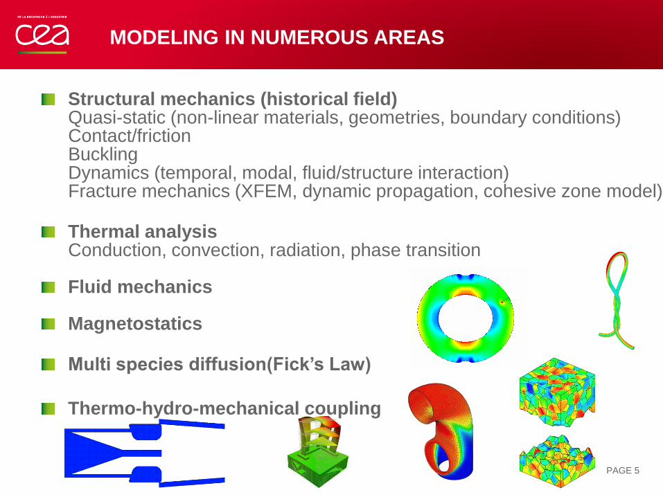
Structural mechanics (historical field)Quasi-static (non-linear materials, geometries, boundary conditions)Contact/frictionBucklingDynamics (temporal, modal, fluid/structure interaction)Fracture mechanics (XFEM, dynamic propagation, cohesive zone model)
Thermal analysisConduction, convection, radiation, phase transition
Fluid mechanics
Magnetostatics
Multi species diffusion(Fick’s Law)
Thermo-hydro-mechanical coupling
THE PASAPAS PROCEDURE
Objective
incremental solving of non linear progressive thermal and mechanical
problems
time can be physical (e.g., thermal transients)
or not (e.g., plasticity with progressive loading)
time or pseudo-time is called the evolution parameter
Non linear phenomena consideredbehavior (plasticity, damage, variable material properties, …) geometry (large displacements)strains (large rotations)boundary conditions (radiation, friction, following pressure, …)
PAGE 6
PASAPAS USE
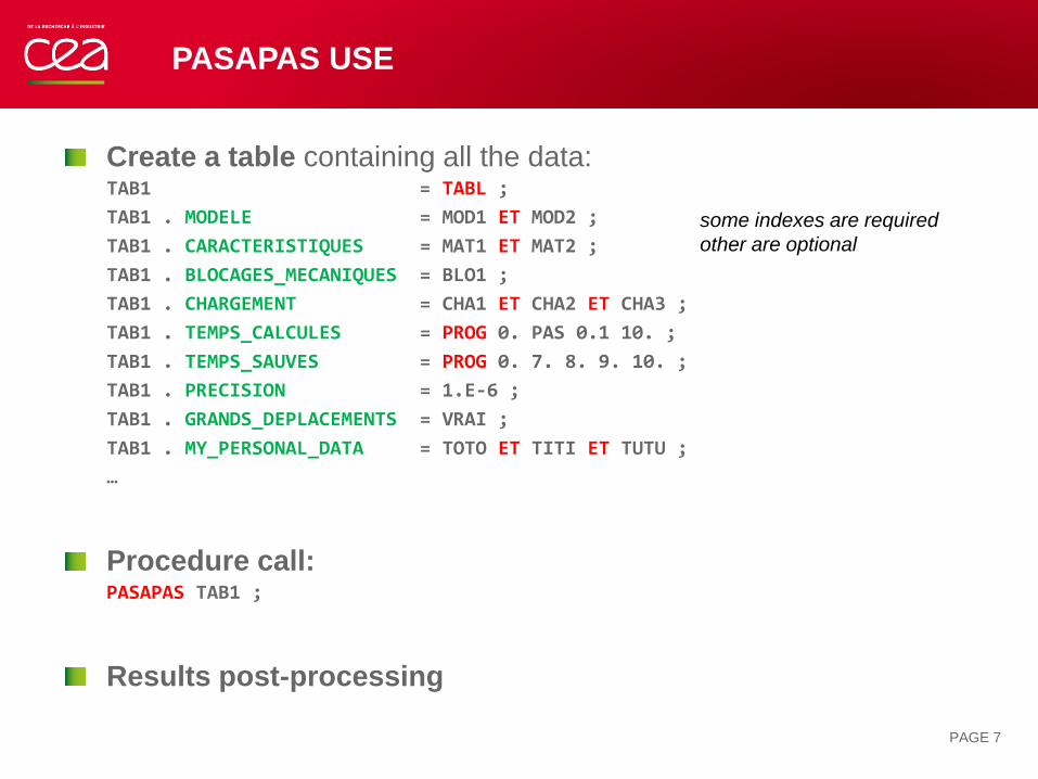
Create a table containing all the data:TAB1 = TABL ;
TAB1 . MODELE = MOD1 ET MOD2 ;
TAB1 . CARACTERISTIQUES = MAT1 ET MAT2 ;
TAB1 . BLOCAGES_MECANIQUES = BLO1 ;
TAB1 . CHARGEMENT = CHA1 ET CHA2 ET CHA3 ;
TAB1 . TEMPS_CALCULES = PROG 0. PAS 0.1 10. ;
TAB1 . TEMPS_SAUVES = PROG 0. 7. 8. 9. 10. ;
TAB1 . PRECISION = 1.E-6 ;
TAB1 . GRANDS_DEPLACEMENTS = VRAI ;
TAB1 . MY_PERSONAL_DATA = TOTO ET TITI ET TUTU ;
…
Procedure call:PASAPAS TAB1 ;
Results post-processing
PAGE 7
some indexes are required
other are optional
OVERVIEW OF INTPUT PARAMETERS
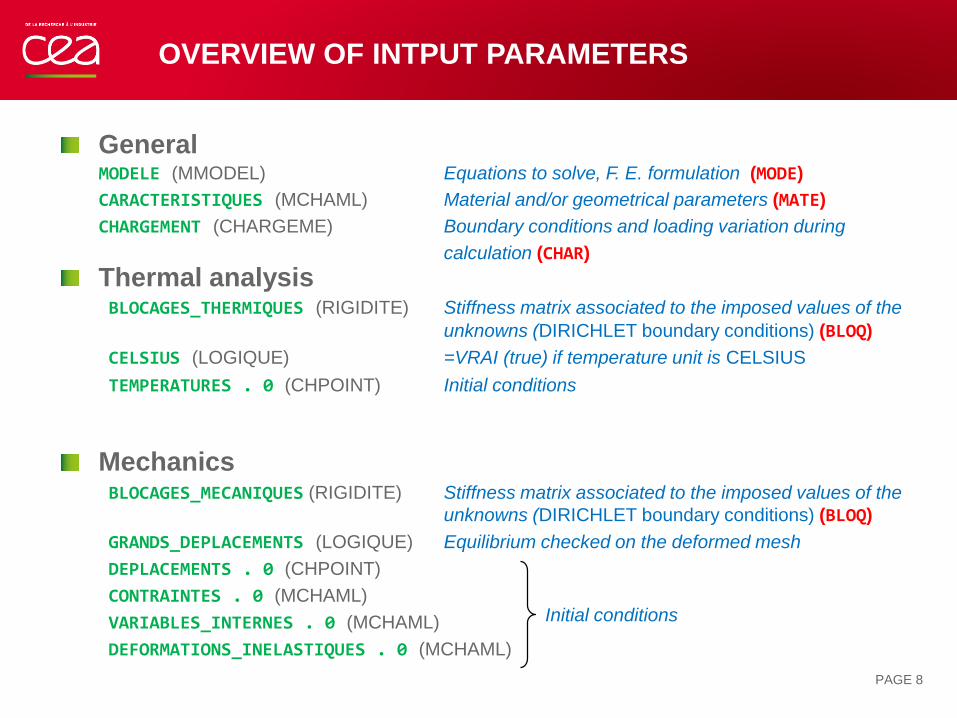
GeneralMODELE (MMODEL) Equations to solve, F. E. formulation (MODE)
CARACTERISTIQUES (MCHAML) Material and/or geometrical parameters (MATE)
CHARGEMENT (CHARGEME) Boundary conditions and loading variation during
calculation (CHAR)
Thermal analysisBLOCAGES_THERMIQUES (RIGIDITE) Stiffness matrix associated to the imposed values of the
unknowns (DIRICHLET boundary conditions) (BLOQ)
CELSIUS (LOGIQUE) =VRAI (true) if temperature unit is CELSIUS
TEMPERATURES . 0 (CHPOINT) Initial conditions
MechanicsBLOCAGES_MECANIQUES (RIGIDITE) Stiffness matrix associated to the imposed values of the
unknowns (DIRICHLET boundary conditions) (BLOQ)
GRANDS_DEPLACEMENTS (LOGIQUE) Equilibrium checked on the deformed mesh
DEPLACEMENTS . 0 (CHPOINT)
CONTRAINTES . 0 (MCHAML)
VARIABLES_INTERNES . 0 (MCHAML)
DEFORMATIONS_INELASTIQUES . 0 (MCHAML)
PAGE 8
Initial conditions
OVERVIEW OF INTPUT PARAMETERS
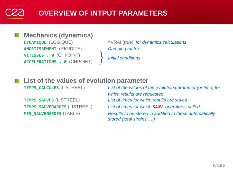
Mechanics (dynamics)DYNAMIQUE (LOGIQUE) =VRAI (true) for dynamics calculations
AMORTISSEMENT (RIGIDITE) Damping matrix
VITESSES . 0 (CHPOINT)
ACCELERATIONS . 0 (CHPOINT)
List of the values of evolution parameter TEMPS_CALCULES (LISTREEL) List of the values of the evolution parameter (or time) for
which results are requested
TEMPS_SAUVES (LISTREEL) List of times for which results are saved
TEMPS_SAUVEGARDES (LISTREEL) List of times for which SAUV operator is called
MES_SAUVEGARDES (TABLE) Results to be stored in addition to those automatically
stored (total strains, …)
PAGE 9
Initial conditions
OVERVIEW OF OUTPUT PARAMETERS
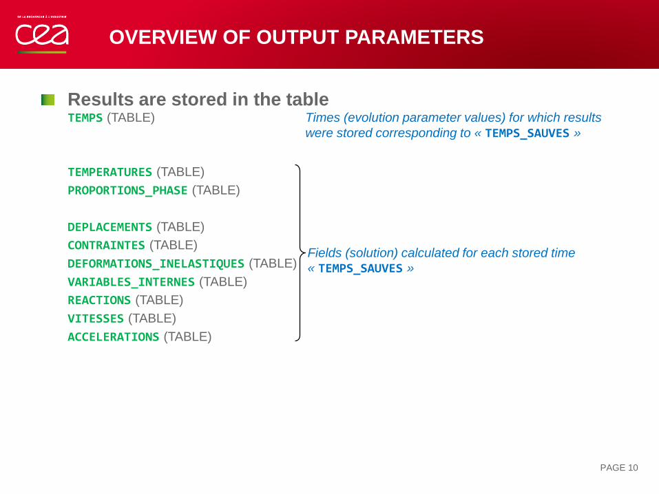
Results are stored in the tableTEMPS (TABLE) Times (evolution parameter values) for which results
were stored corresponding to « TEMPS_SAUVES »
TEMPERATURES (TABLE)
PROPORTIONS_PHASE (TABLE)
DEPLACEMENTS (TABLE)
CONTRAINTES (TABLE)
DEFORMATIONS_INELASTIQUES (TABLE)
VARIABLES_INTERNES (TABLE)
REACTIONS (TABLE)
VITESSES (TABLE)
ACCELERATIONS (TABLE)
PAGE 10
Fields (solution) calculated for each stored time
« TEMPS_SAUVES »
POST PROCESSING (EXAMPLES)
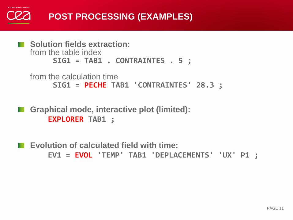
Solution fields extraction:from the table index
SIG1 = TAB1 . CONTRAINTES . 5 ;
from the calculation time SIG1 = PECHE TAB1 'CONTRAINTES' 28.3 ;
Graphical mode, interactive plot (limited):EXPLORER TAB1 ;
Evolution of calculated field with time:EV1 = EVOL 'TEMP' TAB1 'DEPLACEMENTS' 'UX' P1 ;
PAGE 11

PASAPAS OPERATION
PASAPAS OPERATION
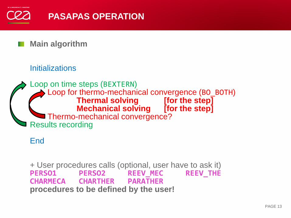
Main algorithm
Initializations
Loop on time steps (BEXTERN)Loop for thermo-mechanical convergence (BO_BOTH)
Thermal solving [for the step]Mechanical solving [for the step]
Thermo-mechanical convergence?Results recording
End
+ User procedures calls (optional, user have to ask it)PERSO1 PERSO2 REEV_MEC REEV_THECHARMECA CHARTHER PARATHERprocedures to be defined by the user!
PAGE 13
PASAPAS OPERATION
PAGE 14
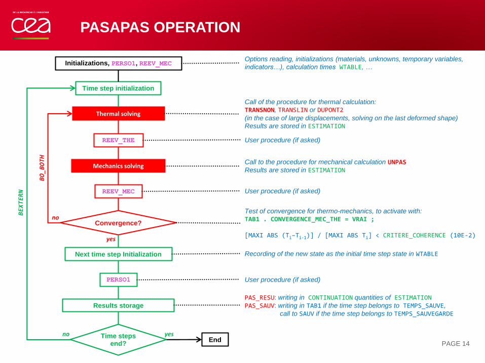
Initializations, PERSO1, REEV_MEC
Time step initialization
REEV_THE
Thermal solving
Mechanics solving
REEV_MEC
Next time step Initialization
PERSO1
Results storage
End
Convergence?
Time steps end?
no
no yes
yes
Options reading, initializations (materials, unknowns, temporary variables,
indicators…), calculation times WTABLE, …
Call of the procedure for thermal calculation:
TRANSNON, TRANSLIN or DUPONT2(in the case of large displacements, solving on the last deformed shape)
Results are stored in ESTIMATION
User procedure (if asked)
Call to the procedure for mechanical calculation UNPASResults are stored in ESTIMATION
User procedure (if asked)
Test of convergence for thermo-mechanics, to activate with:
TAB1 . CONVERGENCE_MEC_THE = VRAI ;
[MAXI ABS (Ti–Ti-1)] / [MAXI ABS Ti] < CRITERE_COHERENCE (10E-2)
User procedure (if asked)
PAS_RESU: writing in CONTINUATION quantities of ESTIMATIONPAS_SAUV: writing in TAB1 if the time step belongs to TEMPS_SAUVE,
call to SAUV if the time step belongs to TEMPS_SAUVEGARDE
Recording of the new state as the initial time step state in WTABLE
BEXTERN
BO_BOTH
ACCESS TO PASAPAS TEMPORARY DATA
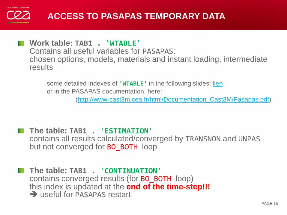
Work table: TAB1 . 'WTABLE'Contains all useful variables for PASAPAS:chosen options, models, materials and instant loading, intermediateresults
some detailed indexes of 'WTABLE' in the following slides: lien
or in the PASAPAS documentation, here:
(http://www-cast3m.cea.fr/html/Documentation_Cast3M/Pasapas.pdf)
The table: TAB1 . 'ESTIMATION'contains all results calculated/converged by TRANSNON and UNPASbut not converged for BO_BOTH loop
The table: TAB1 . 'CONTINUATION'contains converged results (for BO_BOTH loop)this index is updated at the end of the time-step!!! useful for PASAPAS restart
PAGE 15
UNPAS OPERATION
MECHANICAL SOLVER ON A TIME STEP
UNPAS OPERATION
PAGE 17
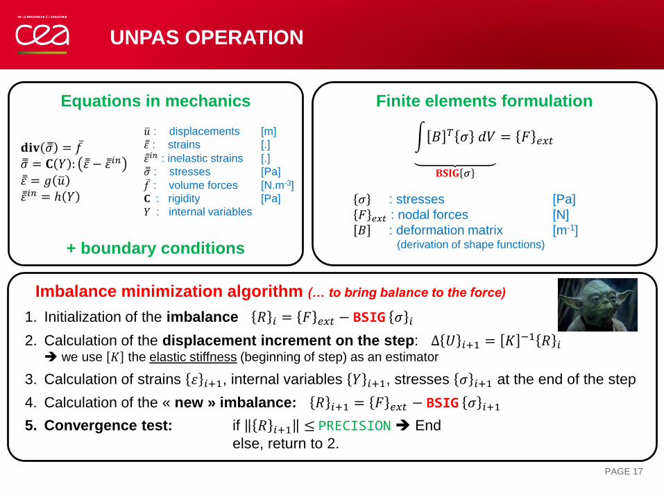
Equations in mechanics
ത𝑢 : displacements [m]
Ӗ𝜀 : strains [.]
Ӗ𝜀𝑖𝑛 : inelastic strains [.]
ധ𝜎 : stresses [Pa]ҧ𝑓 : volume forces [N.m-3]
𝐂 : rigidity [Pa]
𝑌 : internal variables
+ boundary conditions
𝐝𝐢𝐯 ധ𝜎 = ҧ𝑓
ധ𝜎 = 𝐂 𝑌 : Ӗ𝜀 − Ӗ𝜀𝑖𝑛
Ӗ𝜀 = 𝑔 ത𝑢Ӗ𝜀𝑖𝑛 = ℎ 𝑌
Finite elements formulation
𝜎 : stresses [Pa]
𝐹 𝑒𝑥𝑡 : nodal forces [N]
𝐵 : deformation matrix [m-1](derivation of shape functions)
න 𝐵 𝑇 𝜎 𝑑𝑉
𝐁𝐒𝐈𝐆 𝜎
= 𝐹 𝑒𝑥𝑡
Imbalance minimization algorithm (… to bring balance to the force)
1. Initialization of the imbalance 𝑅 𝑖 = 𝐹 𝑒𝑥𝑡 − BSIG 𝜎 𝑖
2. Calculation of the displacement increment on the step: ∆ 𝑈 𝑖+1 = 𝐾 −1 𝑅 𝑖 we use 𝐾 the elastic stiffness (beginning of step) as an estimator
3. Calculation of strains 𝜀 𝑖+1, internal variables 𝑌 𝑖+1, stresses 𝜎 𝑖+1 at the end of the step
4. Calculation of the « new » imbalance: 𝑅 𝑖+1 = 𝐹 𝑒𝑥𝑡 − BSIG 𝜎 𝑖+1
5. Convergence test: if 𝑅 𝑖+1 ≤ PRECISION End
else, return to 2.
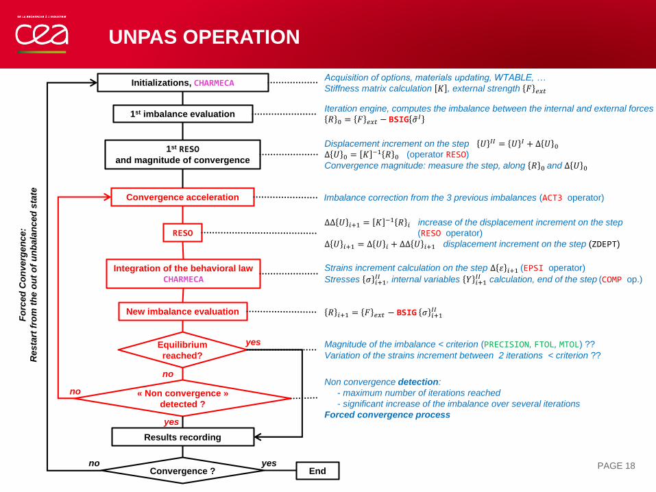
UNPAS OPERATION
PAGE 18
Initializations, CHARMECA
1st imbalance evaluation
1st RESOand magnitude of convergence
RESO
Integration of the behavioral law
CHARMECA
New imbalance evaluation
no
yes
Acquisition of options, materials updating, WTABLE, …
Stiffness matrix calculation 𝐾 , external strength 𝐹 𝑒𝑥𝑡
Displacement increment on the step 𝑈 𝐼𝐼 = 𝑈 𝐼 + ∆ 𝑈 0
∆ 𝑈 0 = 𝐾 −1 𝑅 0 (operator RESO)
Convergence magnitude: measure the step, along 𝑅 0 and ∆ 𝑈 0
∆∆ 𝑈 𝑖+1 = 𝐾 −1 𝑅 𝑖 increase of the displacement increment on the step
(RESO operator)
∆ 𝑈 𝑖+1 = ∆ 𝑈 𝑖 + ∆∆ 𝑈 𝑖+1 displacement increment on the step (ZDEPT)
Magnitude of the imbalance < criterion (PRECISION, FTOL, MTOL) ??
Variation of the strains increment between 2 iterations < criterion ??
Results recording
Equilibrium
reached?
Iteration engine, computes the imbalance between the internal and external forces
𝑅 0 = 𝐹 𝑒𝑥𝑡 − BSIG 𝜎𝐼
Non convergence detection:
- maximum number of iterations reached
- significant increase of the imbalance over several iterations
Forced convergence process
Convergence acceleration
Strains increment calculation on the step ∆ 𝜀 𝑖+1 (EPSI operator)
Stresses 𝜎 𝑖+1𝐼𝐼 , internal variables 𝑌 𝑖+1
𝐼𝐼 calculation, end of the step (COMP op.)
𝑅 𝑖+1 = 𝐹 𝑒𝑥𝑡 − BSIG 𝜎 𝑖+1𝐼𝐼
« Non convergence »
detected ?
no
yes
Endno
Convergence ?
Fo
rced
Co
nverg
en
ce:
Resta
rt f
rom
th
e o
ut
of
un
bala
nced
sta
te
yes
Imbalance correction from the 3 previous imbalances (ACT3 operator)
USERS PROCEDURES
IN PASAPAS
PERSO1 REEV_MEC CHARMECA
PERSO2 REEV_THE CHARTHER PARATHER
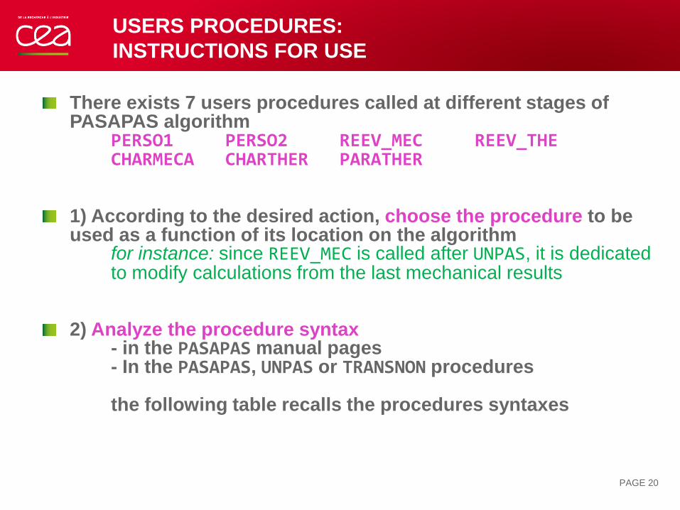
USERS PROCEDURES:
INSTRUCTIONS FOR USE
There exists 7 users procedures called at different stages of PASAPAS algorithm
PERSO1 PERSO2 REEV_MEC REEV_THECHARMECA CHARTHER PARATHER
1) According to the desired action, choose the procedure to be used as a function of its location on the algorithm
for instance: since REEV_MEC is called after UNPAS, it is dedicated to modify calculations from the last mechanical results
2) Analyze the procedure syntax- in the PASAPAS manual pages- In the PASAPAS, UNPAS or TRANSNON procedures
the following table recalls the procedures syntaxes
PAGE 20
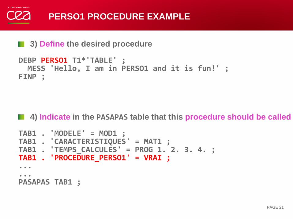
PERSO1 PROCEDURE EXAMPLE
3) Define the desired procedure
DEBP PERSO1 T1*'TABLE' ;MESS 'Hello, I am in PERSO1 and it is fun!' ;
FINP ;
4) Indicate in the PASAPAS table that this procedure should be called
TAB1 . 'MODELE' = MOD1 ;TAB1 . 'CARACTERISTIQUES' = MAT1 ;TAB1 . 'TEMPS_CALCULES' = PROG 1. 2. 3. 4. ;TAB1 . 'PROCEDURE_PERSO1' = VRAI ;......PASAPAS TAB1 ;
PAGE 21
USERS PROCEDURES LIST
PAGE 22
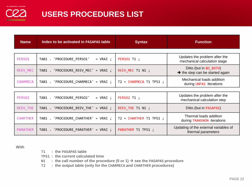
With
T1 : the PASAPAS table
TPS1 : the current calculated time
N1 : the call number of the procedure (0 or 1) see the PASAPAS procedure
T2 : the output table (only for the CHARMECA and CHARTHER procedures)
Name Index to be activated in PASAPAS table Syntax Function
PERSO1 TAB1 . 'PROCEDURE_PERSO1' = VRAI ; PERSO1 T1 ;Updates the problem after the
mechanical calculation stage
REEV_MEC TAB1 . 'PROCEDURE_REEV_MEC' = VRAI ; REEV_MEC T1 N1 ;Ditto (but in BO_BOTH)
the step can be started again
CHARMECA TAB1 . 'PROCEDURE_CHARMECA' = VRAI ; T2 = CHARMECA T1 TPS1 ;Mechanical loads addition
during UNPAS iterations
PERSO2 TAB1 . 'PROCEDURE_PERSO2' = VRAI ; PERSO2 T1 ;Updates the problem after the
mechanical calculation step
REEV_THE TAB1 . 'PROCEDURE_REEV_THE' = VRAI ; REEV_THE T1 N1 ; Ditto (but in PASAPAS)
CHARTHER TAB1 . 'PROCEDURE_CHARTHER' = VRAI ; T2 = CHARTHER T1 TPS1 ;Thermal loads addition
during TRANSNON iterations
PARATHER TAB1 . 'PROCEDURE_PARATHER' = VRAI ; PARATHER T1 TPS1 ;Updating of the external variables of
thermal parameters
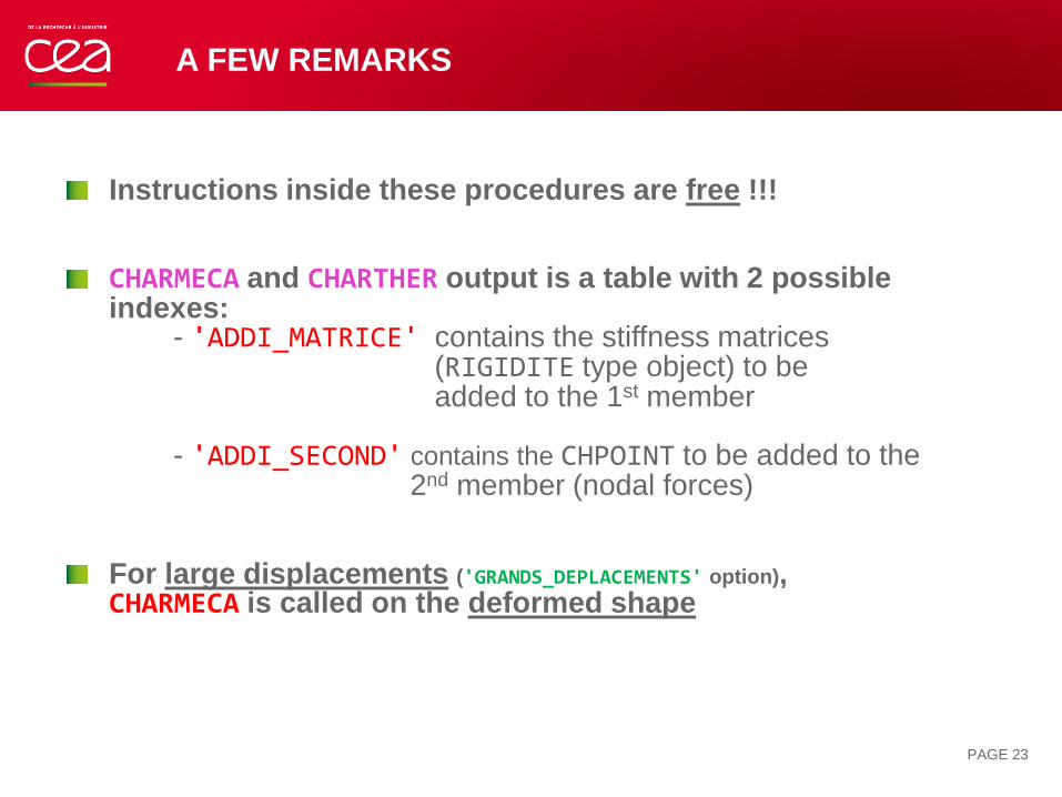
A FEW REMARKS
Instructions inside these procedures are free !!!
CHARMECA and CHARTHER output is a table with 2 possible indexes:
- 'ADDI_MATRICE' contains the stiffness matrices(RIGIDITE type object) to beadded to the 1st member
- 'ADDI_SECOND' contains the CHPOINT to be added to the2nd member (nodal forces)
For large displacements ('GRANDS_DEPLACEMENTS' option),CHARMECA is called on the deformed shape
PAGE 23
EXERCISE 1:
BEAM WITH FOLLOWING FORCE
DOWNLOAD THE STARTING FILE ON THE WEBSITE:
HTTP://WWW-CAST3M.CEA.FR/INDEX.PHP?PAGE=EXEMPLES&EXEMPLE=FORMATION_PASAPAS_1_INITIAL
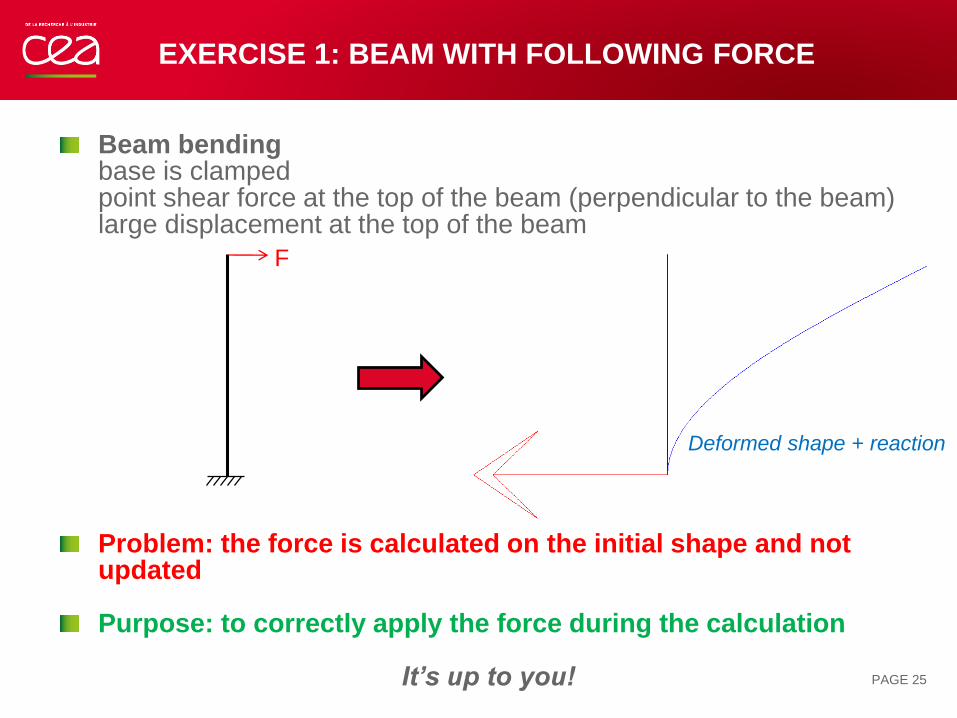
EXERCISE 1: BEAM WITH FOLLOWING FORCE
Beam bendingbase is clamped point shear force at the top of the beam (perpendicular to the beam)large displacement at the top of the beam
Problem: the force is calculated on the initial shape and not updated
Purpose: to correctly apply the force during the calculation
It’s up to you! PAGE 25
Deformed shape + reaction
F
EXERCISE 1: BEAM WITH FOLLOWING FORCE
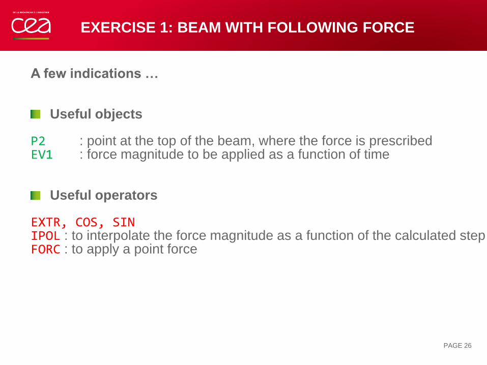
A few indications …
Useful objects
P2 : point at the top of the beam, where the force is prescribedEV1 : force magnitude to be applied as a function of time
Useful operators
EXTR, COS, SINIPOL : to interpolate the force magnitude as a function of the calculated stepFORC : to apply a point force
PAGE 26
EXERCISE 1: BEAM WITH FOLLOWING FORCE
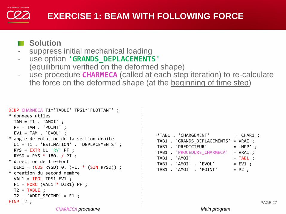
Solution- suppress initial mechanical loading- use option 'GRANDS_DEPLACEMENTS'
(equilibrium verified on the deformed shape)- use procedure CHARMECA (called at each step iteration) to re-calculate
the force on the deformed shape (at the beginning of time step)
PAGE 27
CHARMECA procedure Main program
DEBP CHARMECA T1*'TABLE' TPS1*'FLOTTANT' ;* donnees utilesTAM = T1 . 'AMOI' ;PF = TAM . 'POINT' ;EV1 = TAM . 'EVOL' ;
* angle de rotation de la section droiteU1 = T1 . 'ESTIMATION' . 'DEPLACEMENTS' ;RYS = EXTR U1 'RY' PF ;RYSD = RYS * 180. / PI ;
* direction de l'effortDIR1 = (COS RYSD) 0. (-1. * (SIN RYSD)) ;
* creation du second membreVAL1 = IPOL TPS1 EV1 ;F1 = FORC (VAL1 * DIR1) PF ;T2 = TABLE ;T2 . 'ADDI_SECOND' = F1 ;
FINP T2 ;
*TAB1 . 'CHARGEMENT' = CHAR1 ;TAB1 . 'GRANDS_DEPLACEMENTS' = VRAI ;TAB1 . 'PREDICTEUR' = 'HPP' ;TAB1 . 'PROCEDURE_CHARMECA' = VRAI ;TAB1 . 'AMOI' = TABL ;TAB1 . 'AMOI' . 'EVOL' = EV1 ;TAB1 . 'AMOI' . 'POINT' = P2 ;
EXERCISE 1: BEAM WITH FOLLOWING FORCE
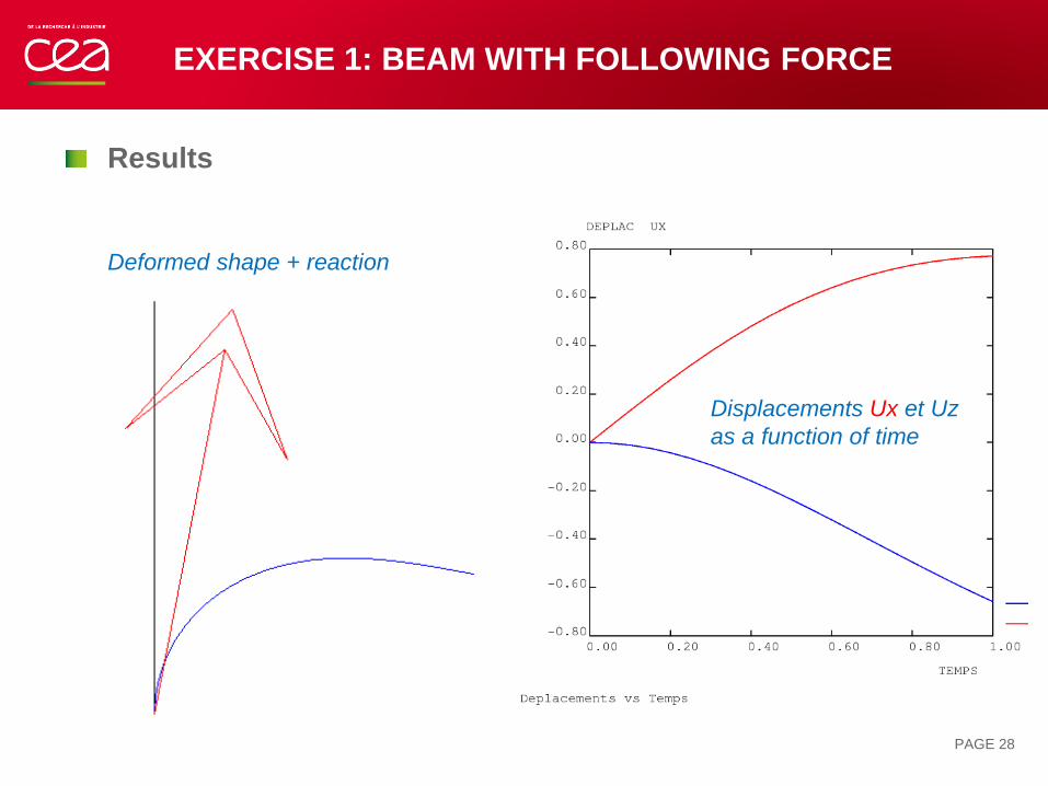
Results
PAGE 28
Displacements Ux et Uz
as a function of time
Deformed shape + reaction
EXERCISE 1: BEAM WITH FOLLOWING FORCE
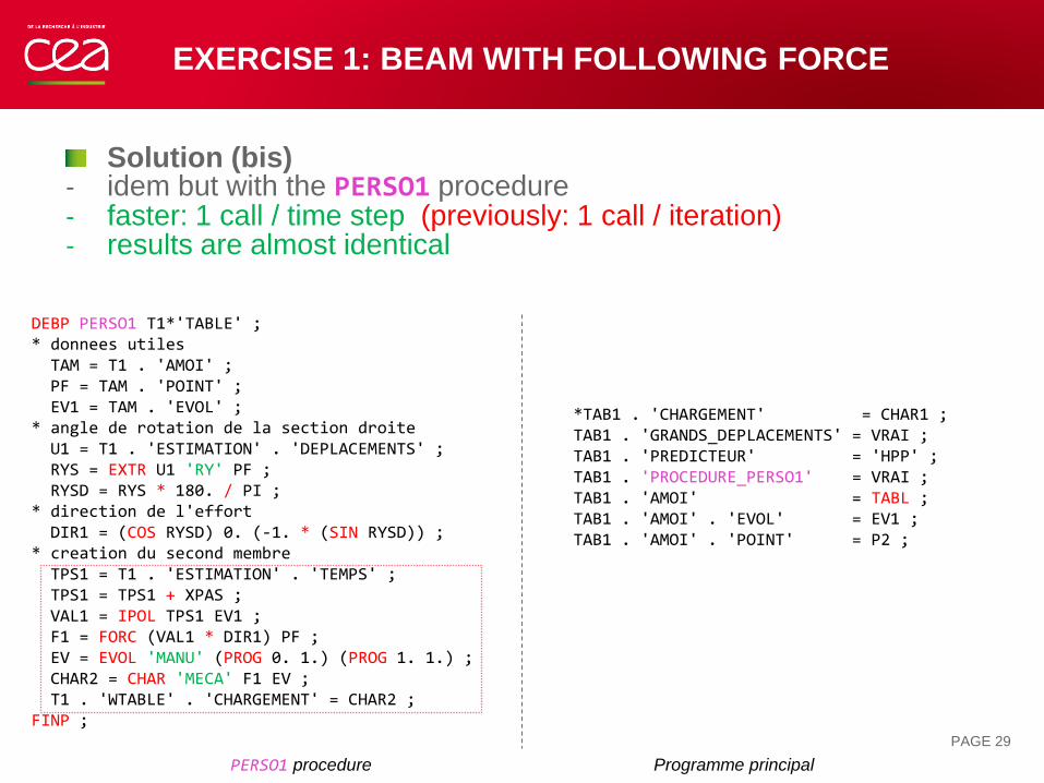
Solution (bis)- idem but with the PERSO1 procedure- faster: 1 call / time step (previously: 1 call / iteration)- results are almost identical
PAGE 29
PERSO1 procedure Programme principal
*TAB1 . 'CHARGEMENT' = CHAR1 ;TAB1 . 'GRANDS_DEPLACEMENTS' = VRAI ;TAB1 . 'PREDICTEUR' = 'HPP' ;TAB1 . 'PROCEDURE_PERSO1' = VRAI ;TAB1 . 'AMOI' = TABL ;TAB1 . 'AMOI' . 'EVOL' = EV1 ;TAB1 . 'AMOI' . 'POINT' = P2 ;
DEBP PERSO1 T1*'TABLE' ;* donnees utilesTAM = T1 . 'AMOI' ;PF = TAM . 'POINT' ;EV1 = TAM . 'EVOL' ;
* angle de rotation de la section droiteU1 = T1 . 'ESTIMATION' . 'DEPLACEMENTS' ;RYS = EXTR U1 'RY' PF ;RYSD = RYS * 180. / PI ;
* direction de l'effortDIR1 = (COS RYSD) 0. (-1. * (SIN RYSD)) ;
* creation du second membreTPS1 = T1 . 'ESTIMATION' . 'TEMPS' ;TPS1 = TPS1 + XPAS ;VAL1 = IPOL TPS1 EV1 ;F1 = FORC (VAL1 * DIR1) PF ;EV = EVOL 'MANU' (PROG 0. 1.) (PROG 1. 1.) ;CHAR2 = CHAR 'MECA' F1 EV ;T1 . 'WTABLE' . 'CHARGEMENT' = CHAR2 ;
FINP ;
EXERCISE 1: BEAM WITH FOLLOWING FORCE
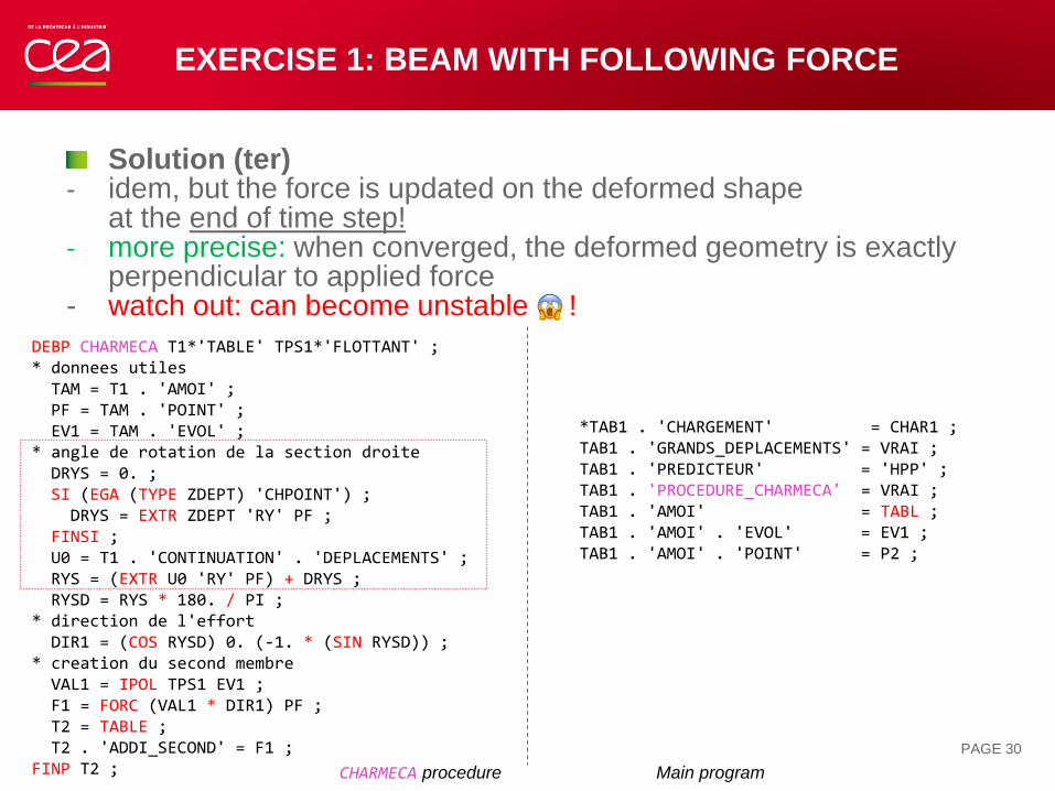
Solution (ter)- idem, but the force is updated on the deformed shape
at the end of time step!- more precise: when converged, the deformed geometry is exactly
perpendicular to applied force- watch out: can become unstable !
PAGE 30
CHARMECA procedure Main program
DEBP CHARMECA T1*'TABLE' TPS1*'FLOTTANT' ;* donnees utilesTAM = T1 . 'AMOI' ;PF = TAM . 'POINT' ;EV1 = TAM . 'EVOL' ;
* angle de rotation de la section droiteDRYS = 0. ;SI (EGA (TYPE ZDEPT) 'CHPOINT') ;
DRYS = EXTR ZDEPT 'RY' PF ;FINSI ;U0 = T1 . 'CONTINUATION' . 'DEPLACEMENTS' ;RYS = (EXTR U0 'RY' PF) + DRYS ;RYSD = RYS * 180. / PI ;
* direction de l'effortDIR1 = (COS RYSD) 0. (-1. * (SIN RYSD)) ;
* creation du second membreVAL1 = IPOL TPS1 EV1 ;F1 = FORC (VAL1 * DIR1) PF ;T2 = TABLE ;T2 . 'ADDI_SECOND' = F1 ;
FINP T2 ;
*TAB1 . 'CHARGEMENT' = CHAR1 ;TAB1 . 'GRANDS_DEPLACEMENTS' = VRAI ;TAB1 . 'PREDICTEUR' = 'HPP' ;TAB1 . 'PROCEDURE_CHARMECA' = VRAI ;TAB1 . 'AMOI' = TABL ;TAB1 . 'AMOI' . 'EVOL' = EV1 ;TAB1 . 'AMOI' . 'POINT' = P2 ;
EXERCISE 2:
RUPTURE BY ELEMENTS REMOVAL
DOWNLOAD THE STARTING FILE ON THE WEBSITE:
HTTP://WWW-CAST3M.CEA.FR/INDEX.PHP?PAGE=EXEMPLES&EXEMPLE=FORMATION_PASAPAS_2_INITIAL
EXERCISE 2: RUPTURE BY ELEMENTS REMOVAL
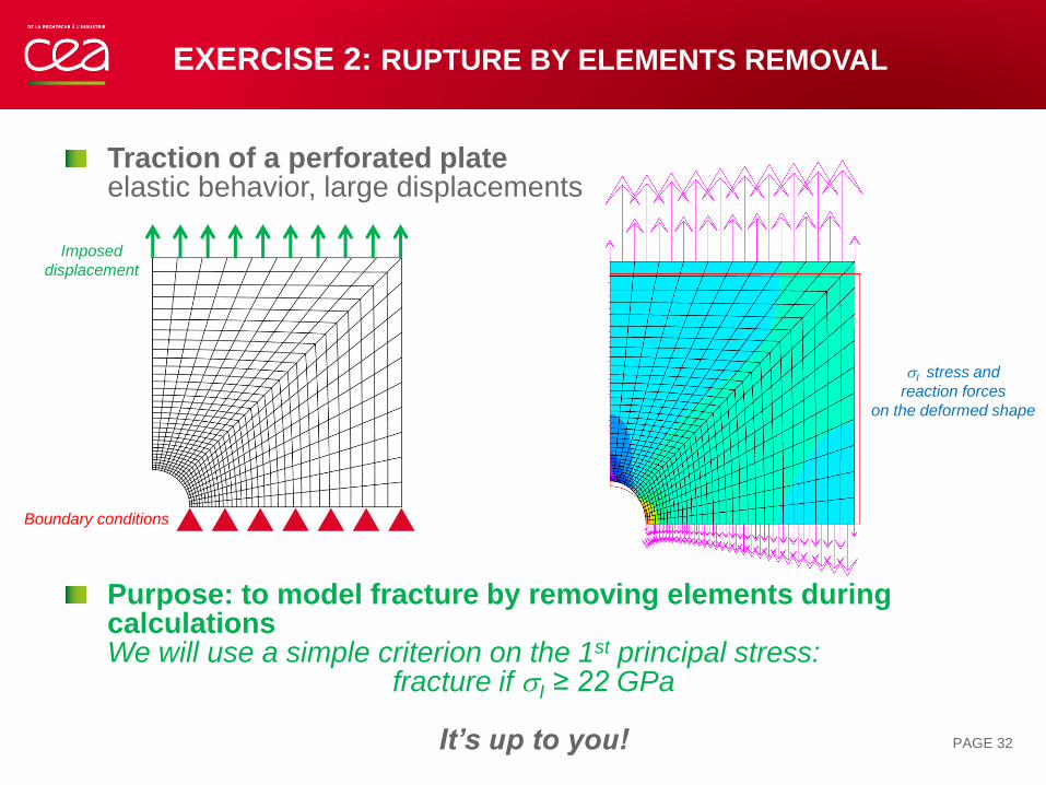
Traction of a perforated plateelastic behavior, large displacements
Purpose: to model fracture by removing elements during calculationsWe will use a simple criterion on the 1st principal stress:
fracture if sI ≥ 22 GPa
It’s up to you! PAGE 32
Imposed
displacement
Boundary conditions
sI stress and
reaction forces
on the deformed shape
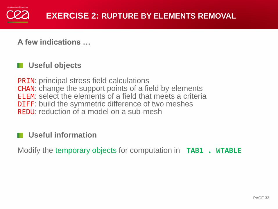
A few indications …
Useful objects
PRIN: principal stress field calculationsCHAN: change the support points of a field by elements ELEM: select the elements of a field that meets a criteriaDIFF: build the symmetric difference of two meshesREDU: reduction of a model on a sub-mesh
Useful information
Modify the temporary objects for computation in TAB1 . WTABLE
PAGE 33
EXERCISE 2: RUPTURE BY ELEMENTS REMOVAL
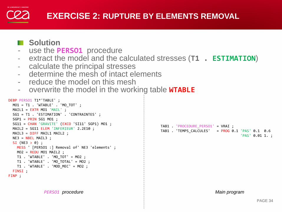
Solution- use the PERSO1 procedure- extract the model and the calculated stresses (T1 . ESTIMATION)- calculate the principal stresses- determine the mesh of intact elements- reduce the model on this mesh- overwrite the model in the working table WTABLE
PAGE 34
EXERCISE 2: RUPTURE BY ELEMENTS REMOVAL
DEBP PERSO1 T1*'TABLE' ;MO1 = T1 . 'WTABLE' . 'MO_TOT' ;MAIL1 = EXTR MO1 'MAIL' ;SG1 = T1 . 'ESTIMATION' . 'CONTRAINTES' ;SGP1 = PRIN SG1 MO1 ;SG11 = CHAN 'GRAVITE' (EXCO 'SI11' SGP1) MO1 ;MAIL2 = SG11 ELEM 'INFERIEUR' 2.2E10 ;MAIL3 = DIFF MAIL1 MAIL2 ;NE3 = NBEL MAIL3 ;SI (NE3 > 0) ;
MESS ' [PERSO1 :] Removal of' NE3 'elements' ;MO2 = REDU MO1 MAIL2 ;T1 . 'WTABLE' . 'MO_TOT' = MO2 ;T1 . 'WTABLE' . 'MO_TOTAL' = MO2 ;T1 . 'WTABLE' . 'MOD_MEC' = MO2 ;
FINSI ;FINP ;
PERSO1 procedure Main program
TAB1 . 'PROCEDURE_PERSO1' = VRAI ;TAB1 . 'TEMPS_CALCULES' = PROG 0.1 'PAS' 0.1 0.6
'PAS' 0.01 1. ;
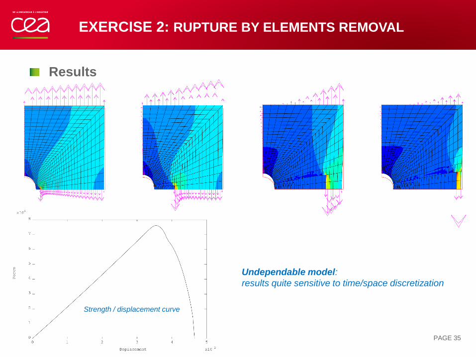
Results
PAGE 35
EXERCISE 2: RUPTURE BY ELEMENTS REMOVAL
Strength / displacement curve
Undependable model:
results quite sensitive to time/space discretization
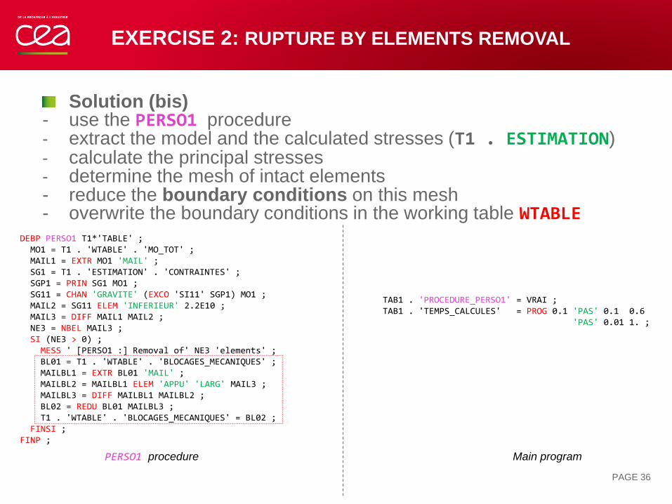
Solution (bis)- use the PERSO1 procedure - extract the model and the calculated stresses (T1 . ESTIMATION)- calculate the principal stresses- determine the mesh of intact elements- reduce the boundary conditions on this mesh- overwrite the boundary conditions in the working table WTABLE
PAGE 36
EXERCISE 2: RUPTURE BY ELEMENTS REMOVAL
DEBP PERSO1 T1*'TABLE' ;MO1 = T1 . 'WTABLE' . 'MO_TOT' ;MAIL1 = EXTR MO1 'MAIL' ;SG1 = T1 . 'ESTIMATION' . 'CONTRAINTES' ;SGP1 = PRIN SG1 MO1 ;SG11 = CHAN 'GRAVITE' (EXCO 'SI11' SGP1) MO1 ;MAIL2 = SG11 ELEM 'INFERIEUR' 2.2E10 ;MAIL3 = DIFF MAIL1 MAIL2 ;NE3 = NBEL MAIL3 ;SI (NE3 > 0) ;
MESS ' [PERSO1 :] Removal of' NE3 'elements' ;BL01 = T1 . 'WTABLE' . 'BLOCAGES_MECANIQUES' ;MAILBL1 = EXTR BL01 'MAIL' ;MAILBL2 = MAILBL1 ELEM 'APPU' 'LARG' MAIL3 ;MAILBL3 = DIFF MAILBL1 MAILBL2 ;BL02 = REDU BL01 MAILBL3 ;T1 . 'WTABLE' . 'BLOCAGES_MECANIQUES' = BL02 ;
FINSI ;FINP ;
PERSO1 procedure Main program
TAB1 . 'PROCEDURE_PERSO1' = VRAI ;TAB1 . 'TEMPS_CALCULES' = PROG 0.1 'PAS' 0.1 0.6
'PAS' 0.01 1. ;
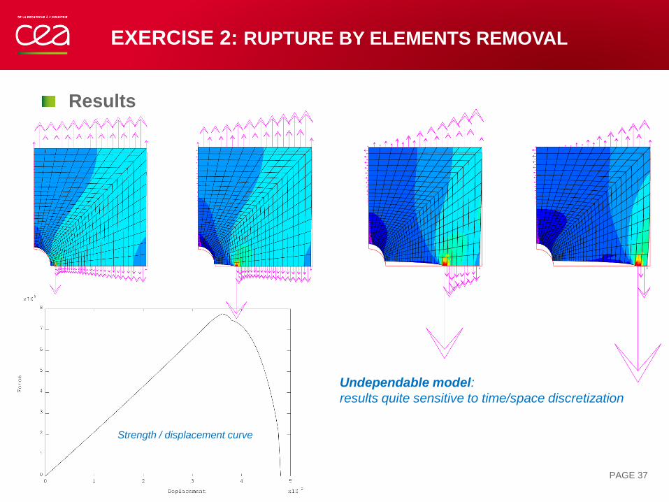
Results
PAGE 37
EXERCISE 2: RUPTURE BY ELEMENTS REMOVAL
Strength / displacement curve
Undependable model:
results quite sensitive to time/space discretization

TRANSNON OPERATION
THERMAL SOLVER

TRANSNON OPERATION
PAGE 39
Heat equation + Fourier’s law
𝑇 : temperature [K]
ത𝑞 : flux density [W.m-2]
𝑡 : time [s]
𝑓 : volumetric source [W.m-3]
𝜌 : mass density [kg.m-3]
𝑐𝑝 : specific heat capacity [J.K-1.kg-1]
𝜆 : thermal conductivity [W.m-1.K-1]
+ boundary conditions
𝜌𝑐𝑝𝜕𝑇
𝜕𝑡+ 𝐝𝐢𝐯 ത𝑞 = 𝑓
ത𝑞 = −𝜆𝐠𝐫𝐚𝐝 𝑇
Finite element formulation
𝑇 : nodal temperatures [K]
𝐹 : nodal flux [W]
𝐶 : capacity matrix [J.K-1]
𝐾 : conductivity matrix [W.K-1]
𝐶 ሶ𝑇 + 𝐾 𝑇 = 𝐹
Time discretization: theta-method (TRANSNON)
𝑇 n+1 : nodal temperatures at time n+1
𝑇 n : nodal temperatures at time n
∆𝑡 : time step
𝜽 : coefficient (𝟎 < 𝜽 < 𝟏)
default value = 1 (implicit scheme)
𝐶 ∗, 𝐾 ∗ and 𝐹 ∗ are estimated:
- at temperature 𝑇 ∗ = 𝜃 𝑇 𝑛+1 + (1 − 𝜃) 𝑇 𝑛
- at time 𝑡∗ = 𝜃𝑡𝑛+1 + (1 − 𝜃)𝑡𝑛
1
Δ𝑡𝐶 ∗. 𝑇 𝑛+1 − 𝑇 𝑛 + 𝐾 ∗. 𝜃 𝑇 𝑛+1 + (1 − 𝜃) 𝑇 𝑛 = 𝐹 ∗
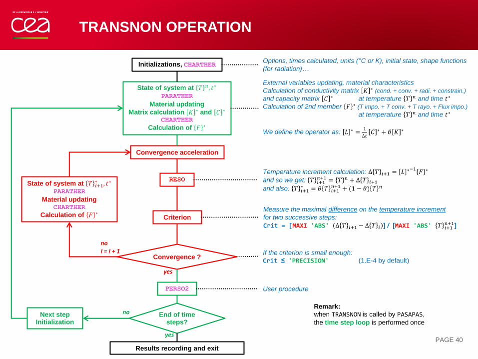
TRANSNON OPERATION
PAGE 40
Initializations, CHARTHER
State of system at 𝑇 𝑛, 𝑡∗
PARATHER
Material updating
Matrix calculation 𝐾 ∗ and 𝐶 ∗
CHARTHER
Calculation of 𝐹 ∗
RESO
PERSO2
Results recording and exit
Convergence ?
End of time steps?
noi = i + 1
no
yes
yes
Options, times calculated, units (°C or K), initial state, shape functions
(for radiation)…
External variables updating, material characteristics
Calculation of conductivity matrix 𝐾 ∗ (cond. + conv. + radi. + constrain.)
and capacity matrix 𝐶 ∗ at temperature 𝑇 𝑛 and time 𝑡∗
Calculation of 2nd member 𝐹 ∗ (T impo. + T conv. + T rayo. + Flux impo.)
at temperature 𝑇 𝑛 and time 𝑡∗
We define the operator as: 𝐿 ∗ =1
∆𝑡𝐶 ∗ + 𝜃 𝐾 ∗
Temperature increment calculation: ∆ 𝑇 𝑖+1 = 𝐿 ∗−1 𝐹 ∗
and so we get: 𝑇 𝑖+1𝑛+1 = 𝑇 𝑛 + ∆ 𝑇 𝑖+1
and also: 𝑇 𝑖+1∗ = 𝜃 𝑇 𝑖+1
𝑛+1 + (1 − 𝜃) 𝑇 𝑛
Measure the maximal difference on the temperature increment
for two successive steps:
Crit = [MAXI 'ABS' ∆ 𝑇 𝑖+1 − ∆ 𝑇 𝑖 ] / [MAXI 'ABS' 𝑇 𝑖+1𝑛+1]
User procedure
State of system at 𝑇 𝑖+1∗ , 𝑡∗
PARATHER
Material updatingCHARTHER
Calculation of 𝐹 ∗
Next step Initialization
Remark:
when TRANSNON is called by PASAPAS,
the time step loop is performed once
Convergence acceleration
Criterion
If the criterion is small enough:
Crit ≤ 'PRECISION' (1.E-4 by default)
EXERCISE 3:
HEAT SOURCE DEPENDING ON TEMPERATURE
DOWNLOAD THE STARTING FILE ON THE WEBSITE:
HTTP://WWW-CAST3M.CEA.FR/INDEX.PHP?PAGE=EXEMPLES&EXEMPLE=FORMATION_PASAPAS_3_INITIAL
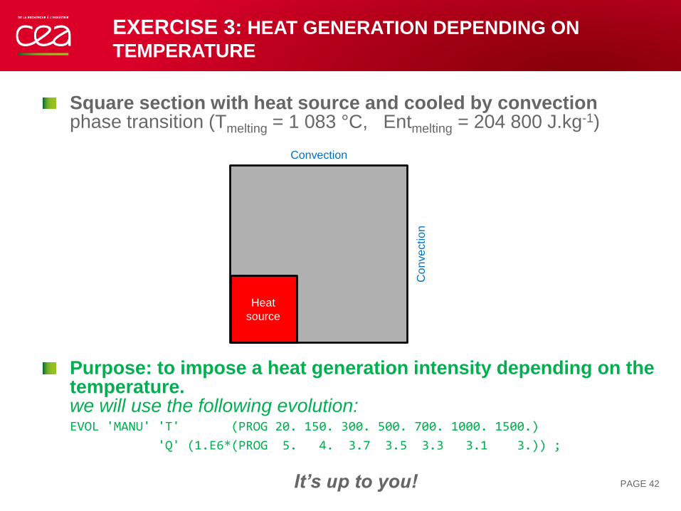
EXERCISE 3: HEAT GENERATION DEPENDING ON
TEMPERATURE
Square section with heat source and cooled by convectionphase transition (Tmelting = 1 083 °C, Entmelting = 204 800 J.kg-1)
Purpose: to impose a heat generation intensity depending on the temperature.we will use the following evolution:EVOL 'MANU' 'T' (PROG 20. 150. 300. 500. 700. 1000. 1500.)
'Q' (1.E6*(PROG 5. 4. 3.7 3.5 3.3 3.1 3.)) ;
It’s up to you! PAGE 42
Heat
source
Convection
Con
ve
ctio
n
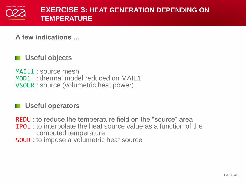
A few indications …
Useful objects
MAIL1 : source mesh MOD1 : thermal model reduced on MAIL1VSOUR : source (volumetric heat power)
Useful operators
REDU : to reduce the temperature field on the "source“ areaIPOL : to interpolate the heat source value as a function of the
computed temperatureSOUR : to impose a volumetric heat source
PAGE 43
EXERCISE 3: HEAT GENERATION DEPENDING ON
TEMPERATURE
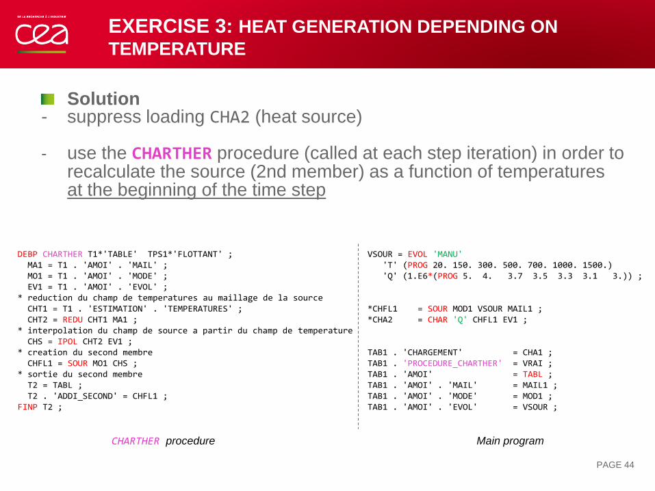
Solution- suppress loading CHA2 (heat source)
- use the CHARTHER procedure (called at each step iteration) in order to recalculate the source (2nd member) as a function of temperaturesat the beginning of the time step
PAGE 44
CHARTHER procedure Main program
EXERCISE 3: HEAT GENERATION DEPENDING ON
TEMPERATURE
VSOUR = EVOL 'MANU''T' (PROG 20. 150. 300. 500. 700. 1000. 1500.)'Q' (1.E6*(PROG 5. 4. 3.7 3.5 3.3 3.1 3.)) ;
*CHFL1 = SOUR MOD1 VSOUR MAIL1 ;*CHA2 = CHAR 'Q' CHFL1 EV1 ;
TAB1 . 'CHARGEMENT' = CHA1 ;TAB1 . 'PROCEDURE_CHARTHER' = VRAI ;TAB1 . 'AMOI' = TABL ;TAB1 . 'AMOI' . 'MAIL' = MAIL1 ;TAB1 . 'AMOI' . 'MODE' = MOD1 ;TAB1 . 'AMOI' . 'EVOL' = VSOUR ;
DEBP CHARTHER T1*'TABLE' TPS1*'FLOTTANT' ;MA1 = T1 . 'AMOI' . 'MAIL' ;MO1 = T1 . 'AMOI' . 'MODE' ;EV1 = T1 . 'AMOI' . 'EVOL' ;
* reduction du champ de temperatures au maillage de la sourceCHT1 = T1 . 'ESTIMATION' . 'TEMPERATURES' ;CHT2 = REDU CHT1 MA1 ;
* interpolation du champ de source a partir du champ de temperatureCHS = IPOL CHT2 EV1 ;
* creation du second membreCHFL1 = SOUR MO1 CHS ;
* sortie du second membreT2 = TABL ;T2 . 'ADDI_SECOND' = CHFL1 ;
FINP T2 ;
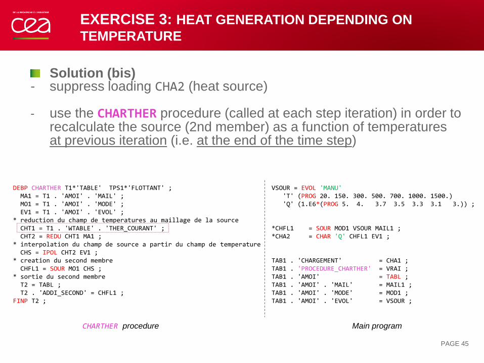
Solution (bis)- suppress loading CHA2 (heat source)
- use the CHARTHER procedure (called at each step iteration) in order to recalculate the source (2nd member) as a function of temperaturesat previous iteration (i.e. at the end of the time step)
PAGE 45
CHARTHER procedure Main program
EXERCISE 3: HEAT GENERATION DEPENDING ON
TEMPERATURE
VSOUR = EVOL 'MANU''T' (PROG 20. 150. 300. 500. 700. 1000. 1500.)'Q' (1.E6*(PROG 5. 4. 3.7 3.5 3.3 3.1 3.)) ;
*CHFL1 = SOUR MOD1 VSOUR MAIL1 ;*CHA2 = CHAR 'Q' CHFL1 EV1 ;
TAB1 . 'CHARGEMENT' = CHA1 ;TAB1 . 'PROCEDURE_CHARTHER' = VRAI ;TAB1 . 'AMOI' = TABL ;TAB1 . 'AMOI' . 'MAIL' = MAIL1 ;TAB1 . 'AMOI' . 'MODE' = MOD1 ;TAB1 . 'AMOI' . 'EVOL' = VSOUR ;
DEBP CHARTHER T1*'TABLE' TPS1*'FLOTTANT' ;MA1 = T1 . 'AMOI' . 'MAIL' ;MO1 = T1 . 'AMOI' . 'MODE' ;EV1 = T1 . 'AMOI' . 'EVOL' ;
* reduction du champ de temperatures au maillage de la sourceCHT1 = T1 . 'WTABLE' . 'THER_COURANT' ;CHT2 = REDU CHT1 MA1 ;
* interpolation du champ de source a partir du champ de temperatureCHS = IPOL CHT2 EV1 ;
* creation du second membreCHFL1 = SOUR MO1 CHS ;
* sortie du second membreT2 = TABL ;T2 . 'ADDI_SECOND' = CHFL1 ;
FINP T2 ;
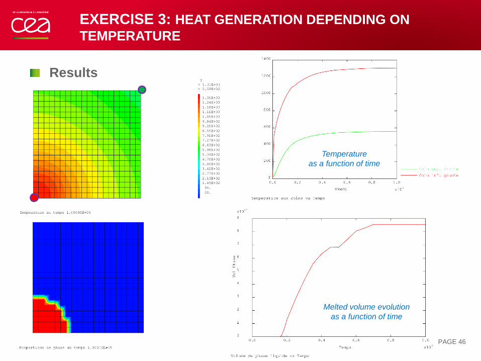
Results
PAGE 46
EXERCISE 3: HEAT GENERATION DEPENDING ON
TEMPERATURE
Temperature
as a function of time
Melted volume evolution
as a function of time
EXERCISE 4:
THERMO-MECHANICAL GAP CLOSING
DOWNLOAD THE STARTING FILE ON THE WEBSITE:
HTTP://WWW-CAST3M.CEA.FR/INDEX.PHP?PAGE=EXEMPLES&EXEMPLE=FORMATION_PASAPAS_4_INITIAL
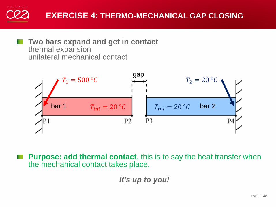
EXERCISE 4: THERMO-MECHANICAL GAP CLOSING
Two bars expand and get in contactthermal expansion unilateral mechanical contact
Purpose: add thermal contact, this is to say the heat transfer when the mechanical contact takes place.
It’s up to you!
PAGE 48
𝑇1 = 500 °𝐶 𝑇2 = 20 °𝐶
𝑇𝑖𝑛𝑖 = 20 °𝐶𝑇𝑖𝑛𝑖 = 20 °𝐶
gap
bar 1 bar 2
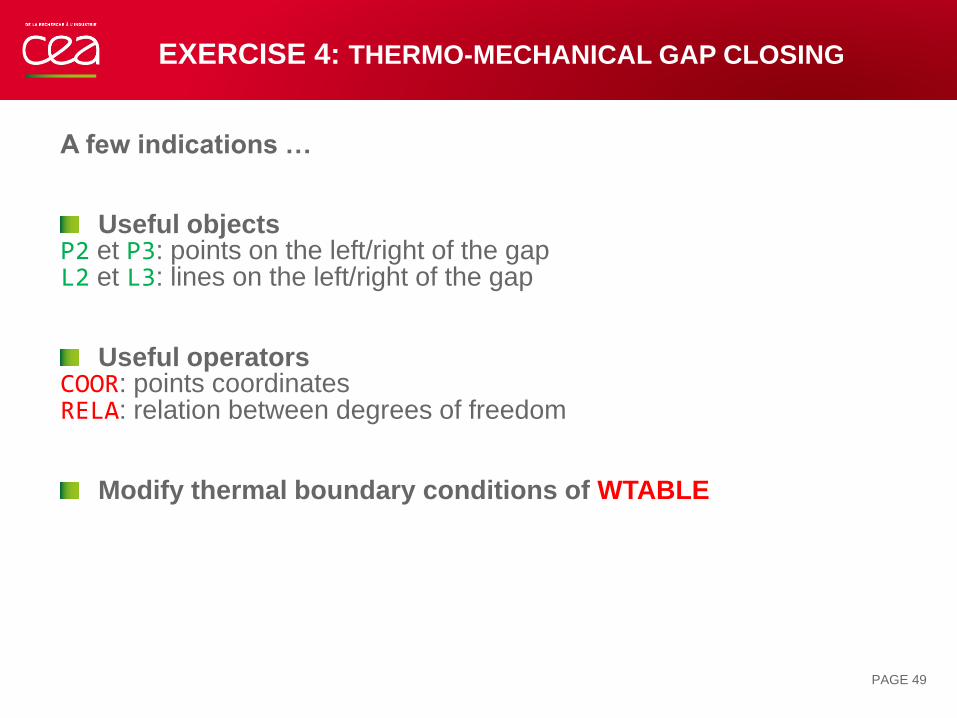
A few indications …
Useful objectsP2 et P3: points on the left/right of the gapL2 et L3: lines on the left/right of the gap
Useful operatorsCOOR: points coordinates RELA: relation between degrees of freedom
Modify thermal boundary conditions of WTABLE
PAGE 49
EXERCISE 4: THERMO-MECHANICAL GAP CLOSING
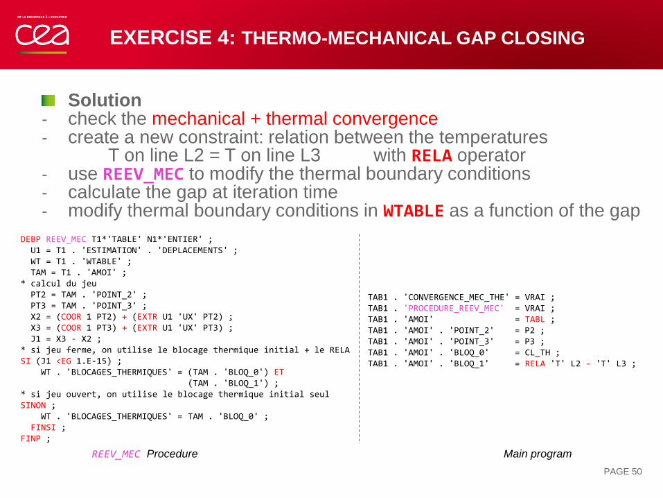
Solution- check the mechanical + thermal convergence- create a new constraint: relation between the temperatures
T on line L2 = T on line L3 with RELA operator- use REEV_MEC to modify the thermal boundary conditions- calculate the gap at iteration time- modify thermal boundary conditions in WTABLE as a function of the gap
PAGE 50
REEV_MEC Procedure Main program
EXERCISE 4: THERMO-MECHANICAL GAP CLOSING
DEBP REEV_MEC T1*'TABLE' N1*'ENTIER' ;U1 = T1 . 'ESTIMATION' . 'DEPLACEMENTS' ;WT = T1 . 'WTABLE' ;TAM = T1 . 'AMOI' ;
* calcul du jeuPT2 = TAM . 'POINT_2' ;PT3 = TAM . 'POINT_3' ;X2 = (COOR 1 PT2) + (EXTR U1 'UX' PT2) ;X3 = (COOR 1 PT3) + (EXTR U1 'UX' PT3) ;J1 = X3 - X2 ;
* si jeu ferme, on utilise le blocage thermique initial + le RELASI (J1 <EG 1.E-15) ;
WT . 'BLOCAGES_THERMIQUES' = (TAM . 'BLOQ_0') ET(TAM . 'BLOQ_1') ;
* si jeu ouvert, on utilise le blocage thermique initial seulSINON ;
WT . 'BLOCAGES_THERMIQUES' = TAM . 'BLOQ_0' ;FINSI ;
FINP ;
TAB1 . 'CONVERGENCE_MEC_THE' = VRAI ;TAB1 . 'PROCEDURE_REEV_MEC' = VRAI ;TAB1 . 'AMOI' = TABL ;TAB1 . 'AMOI' . 'POINT_2' = P2 ;TAB1 . 'AMOI' . 'POINT_3' = P3 ;TAB1 . 'AMOI' . 'BLOQ_0' = CL_TH ;TAB1 . 'AMOI' . 'BLOQ_1' = RELA 'T' L2 - 'T' L3 ;
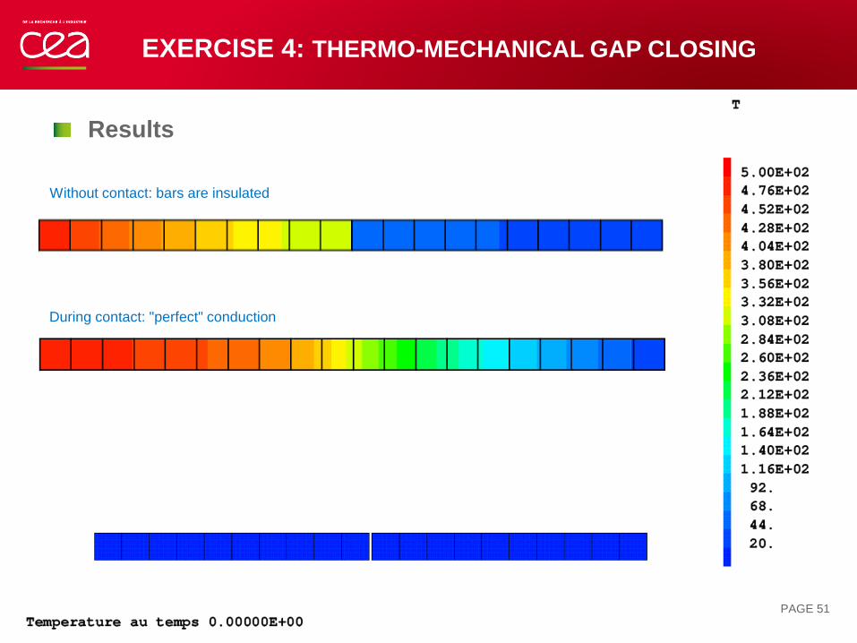
Results
PAGE 51
During contact: "perfect" conduction
Without contact: bars are insulated
EXERCISE 4: THERMO-MECHANICAL GAP CLOSING
EXERCISE 4: THERMO-MECHANICAL GAP CLOSING
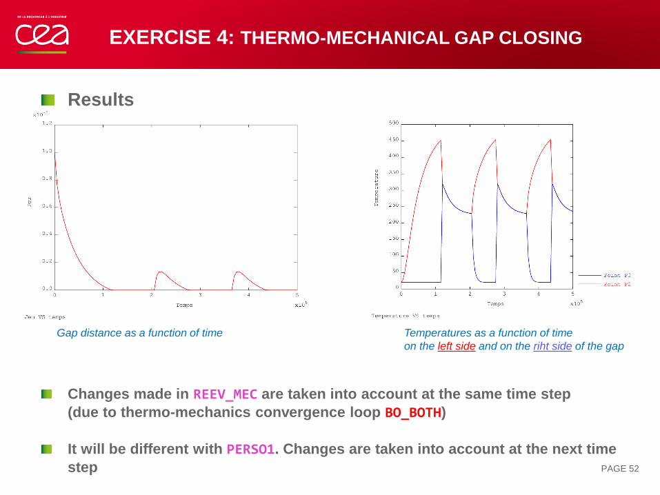
Results
Changes made in REEV_MEC are taken into account at the same time step
(due to thermo-mechanics convergence loop BO_BOTH)
It will be different with PERSO1. Changes are taken into account at the next time
step
Temperatures as a function of time
on the left side and on the riht side of the gap
Gap distance as a function of time
PAGE 52
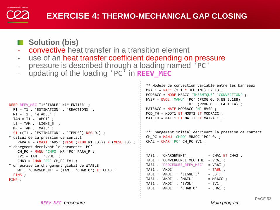
Solution (bis)- convective heat transfer in a transition element- use of an heat transfer coefficient depending on pressure- pressure is described through a loading named 'PC'- updating of the loading 'PC' in REEV_MEC
PAGE 53REEV_MEC procedure Main program
EXERCISE 4: THERMO-MECHANICAL GAP CLOSING
** Modele de convection variable entre les barreauxMRACC = RACC (1.1 * JEU_INI) L2 L3 ;MODRACC = MODE MRACC 'THERMIQUE' 'CONVECTION' ;HVSP = EVOL 'MANU' 'PC' (PROG 0. 5.E8 5.1E8)
'H' (PROG 0. 1.E4 1.E4) ;MATRACC = MATE MODRACC 'H' HVSP ;MOD_TH = MODT1 ET MODT2 ET MODRACC ;MAT_TH = MATT1 ET MATT2 ET MATRACC ;
** Chargement initial decrivant la pression de contactCH_PC = MANU 'CHPO' MRACC 'PC' 0. ;CHA2 = CHAR 'PC' CH_PC EV1 ;
TAB1 . 'CHARGEMENT' = CHA1 ET CHA2 ;TAB1 . 'CONVERGENCE_MEC_THE' = VRAI ;TAB1 . 'PROCEDURE_REEV_MEC' = VRAI ;TAB1 . 'AMOI' = TABL ;TAB1 . 'AMOI' . 'LIGNE_3' = L3 ;TAB1 . 'AMOI' . 'MAIL' = MRACC ;TAB1 . 'AMOI' . 'EVOL' = EV1 ;TAB1 . 'AMOI' . 'CHAR_0' = CHA1 ;
DEBP REEV_MEC T1*'TABLE' N1*'ENTIER' ;R1 = T1 . 'ESTIMATION' . 'REACTIONS' ;WT = T1 . 'WTABLE' ;TAM = T1 . 'AMOI' ;L3 = TAM . 'LIGNE_3' ;MR = TAM . 'MAIL' ;SI ((T1 . 'ESTIMATION' . 'TEMPS') NEG 0.) ;
* calcul de la pression de contactPARA_P = (MAXI 'ABS' (RESU (REDU R1 L3))) / (MESU L3) ;
* chargment decrivant le parametre 'PC'CH_PC = MANU 'CHPO' MR 'PC' PARA_P ;EV1 = TAM . 'EVOL' ;CHA3 = CHAR 'PC' CH_PC EV1 ;
* on ecrase le chargement global de WTABLEWT . 'CHARGEMENT' = (TAM . 'CHAR_0') ET CHA3 ;
FINS ;FINP ;
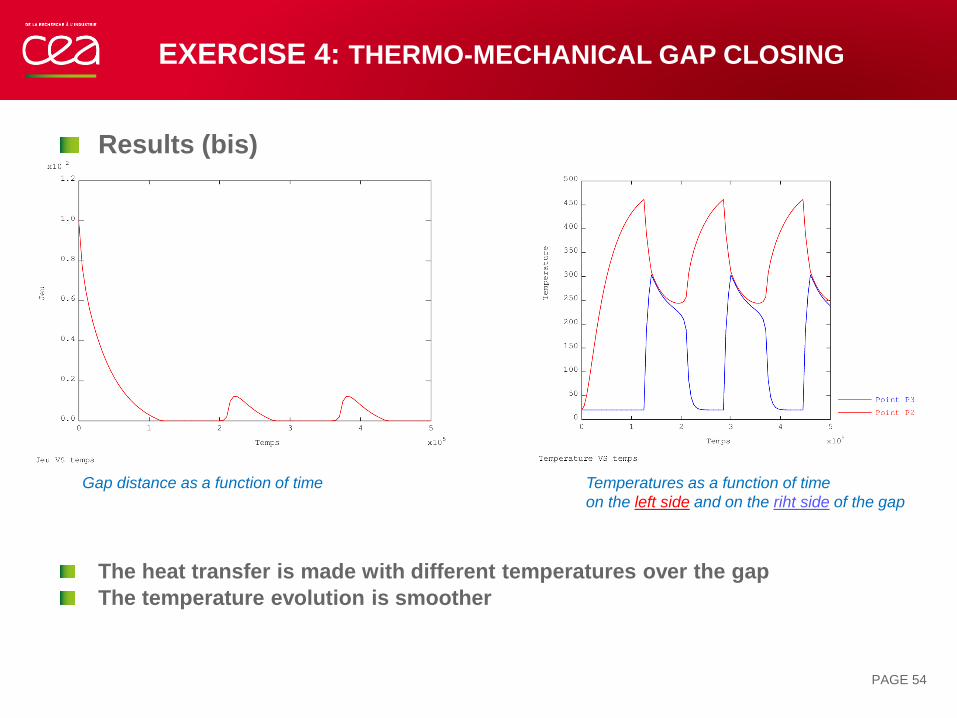
Results (bis)
The heat transfer is made with different temperatures over the gap
The temperature evolution is smoother
PAGE 54
EXERCISE 4: THERMO-MECHANICAL GAP CLOSING
Temperatures as a function of time
on the left side and on the riht side of the gap
Gap distance as a function of time

ANNEXES
ANNEX: A FEW INDEXES OF WTABLE
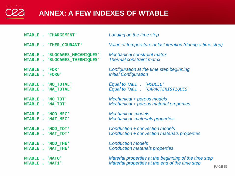
WTABLE . 'CHARGEMENT' Loading on the time step
WTABLE . 'THER_COURANT‘ Value of temperature at last iteration (during a time step)
WTABLE . 'BLOCAGES_MECANIQUES' Mechanical constraint matrixWTABLE . 'BLOCAGES_THERMIQUES' Thermal constraint matrix
WTABLE . 'FOR' Configuration at the time step beginning WTABLE . 'FOR0' Initial Configuration
WTABLE . 'MO_TOTAL' Equal to TAB1 . 'MODELE'WTABLE . 'MA_TOTAL' Equal to TAB1 . 'CARACTERISTIQUES'
WTABLE . 'MO_TOT' Mechanical + porous models WTABLE . 'MA_TOT' Mechanical + porous material properties
WTABLE . 'MOD_MEC' Mechanical models WTABLE . 'MAT_MEC' Mechanical materials properties
WTABLE . 'MOD_TOT‘ Conduction + convection modelsWTABLE . 'MAT_TOT' Conduction + convection materials properties
WTABLE . 'MOD_THE' Conduction modelsWTABLE . 'MAT_THE' Conduction materials properties
WTABLE . 'MAT0' Material properties at the beginning of the time stepWTABLE . 'MAT1' Material properties at the end of the time step
PAGE 56
ANNEX: ALGORITHMIC CONTROL PARAMETERS
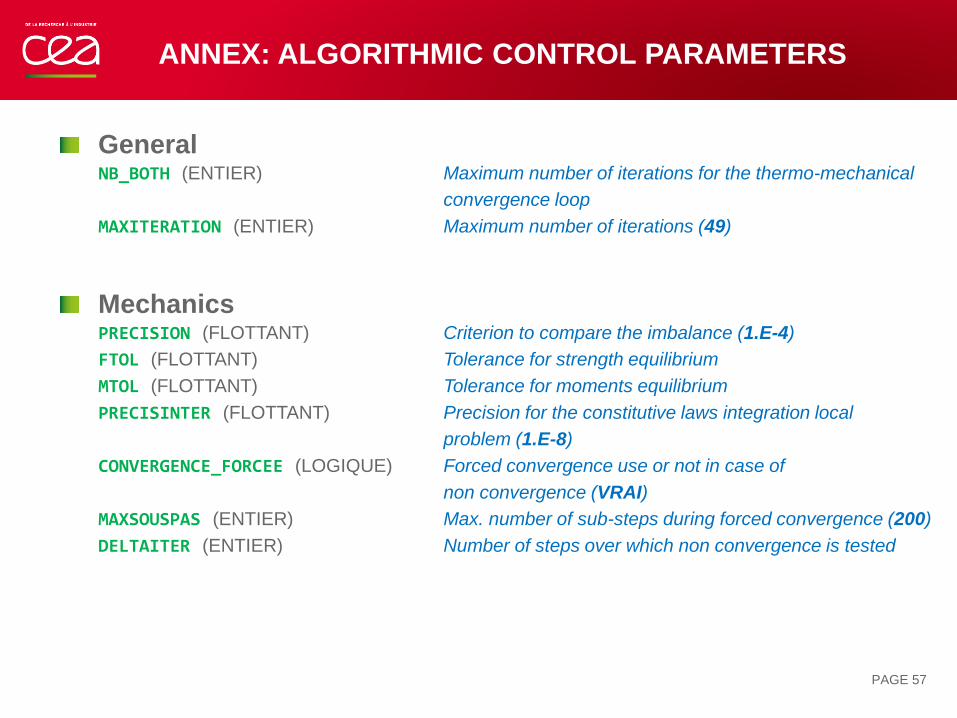
GeneralNB_BOTH (ENTIER) Maximum number of iterations for the thermo-mechanical
convergence loop
MAXITERATION (ENTIER) Maximum number of iterations (49)
MechanicsPRECISION (FLOTTANT) Criterion to compare the imbalance (1.E-4)
FTOL (FLOTTANT) Tolerance for strength equilibrium
MTOL (FLOTTANT) Tolerance for moments equilibrium
PRECISINTER (FLOTTANT) Precision for the constitutive laws integration local
problem (1.E-8)
CONVERGENCE_FORCEE (LOGIQUE) Forced convergence use or not in case of
non convergence (VRAI)
MAXSOUSPAS (ENTIER) Max. number of sub-steps during forced convergence (200)
DELTAITER (ENTIER) Number of steps over which non convergence is tested
PAGE 57
ANNEX: ALGORITHMIC CONTROL PARAMETERS
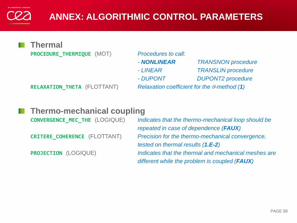
ThermalPROCEDURE_THERMIQUE (MOT) Procedures to call:
- NONLINEAR TRANSNON procedure
- LINEAR TRANSLIN procedure
- DUPONT DUPONT2 procedure
RELAXATION_THETA (FLOTTANT) Relaxation coefficient for the q-method (1)
Thermo-mechanical couplingCONVERGENCE_MEC_THE (LOGIQUE) Indicates that the thermo-mechanical loop should be
repeated in case of dependence (FAUX)
CRITERE_COHERENCE (FLOTTANT) Precision for the thermo-mechanical convergence,
tested on thermal results (1.E-2)
PROJECTION (LOGIQUE) Indicates that the thermal and mechanical meshes are
different while the problem is coupled (FAUX)
PAGE 58
ANNEX: LARGE DISPLACEMENTS
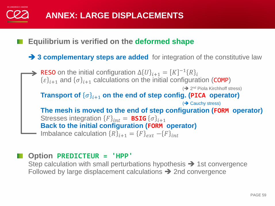
Equilibrium is verified on the deformed shape
3 complementary steps are added for integration of the constitutive law
RESO on the initial configuration ∆ 𝑈 𝑖+1 = 𝐾 −1 𝑅 𝑖𝜀 𝑖+1 and 𝜎 𝑖+1 calculations on the initial configuration (COMP)
( 2nd Piola Kirchhoff stress)
Transport of 𝜎 𝑖+1 on the end of step config. (PICA operator)( Cauchy stress)
The mesh is moved to the end of step configuration (FORM operator)Stresses integration 𝐹 𝑖𝑛𝑡 = BSIG 𝜎 𝑖+1Back to the initial configuration (FORM operator)Imbalance calculation 𝑅 𝑖+1 = 𝐹 𝑒𝑥𝑡 − 𝐹 𝑖𝑛𝑡
Option PREDICTEUR = 'HPP'Step calculation with small perturbations hypothesis 1st convergenceFollowed by large displacement calculations 2nd convergence
PAGE 59
ANNEX: CONVERGENCE CRITERION (UNPAS)
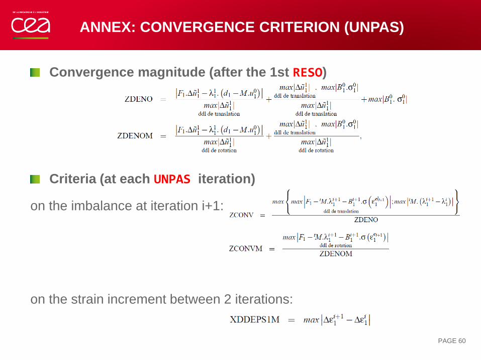
Convergence magnitude (after the 1st RESO)
Criteria (at each UNPAS iteration)
on the imbalance at iteration i+1:
on the strain increment between 2 iterations:
PAGE 60
ANNEX: FORCED CONVERGENCE
If non convergence is confirmed, the step is re-calculated:
- state at the beginning of the step is redefined- the last “out of equilibrium“ state with minimal imbalance is chosen- at the beginning of time step, are overwritten:
- the instant- the material properties- the displacements- the internal variables- the inelastic strains - the stresses
- UNPAS is re-started with a time-step equal to zero- no load increment, only disequilibrium
- allows to find a solution with the right behavior and equilibriumbut with a different loading path
PAGE 61

DEN/DANS
DM2S
SEMT
François DI PAOLA
Commissariat à l'énergie atomique et aux énergies alternatives
Centre de Saclay | 91191 Gif-sur-Yvette Cedex
Etablissement public à caractère industriel et commercial | R.C.S Paris B 775 685 019