The patterns of output growth of firms

and countries: new evidence on

scale invariances and scale specificities∗

Carolina Castaldi† Giovanni Dosi‡

23rd April 2007

∗The authors wish to thank Giulio Bottazzi, Buz Brock, Alessandro Nuvolari, Bart Los, Angelo

Secchi, Gerry Silverberg, Eddy Szirmai and Bart Verspagen for helpful discussions, and several partici-

pants at the conferences “Economic Growth and Distribution”, Lucca, 2004 and “Dynamics, Economic

Growth and International Trade (DEGIT IX)”, Reykjavik, 2004, for their comments. An anonymous

referee and the editor helped to substantially improve the paper. We gratefully acknowledge sup-

port from the Robert Solow Post-doctoral Fellowship of Cournot Center for Economic Studies (to C.

Castaldi) and from the Italian Ministry for University and Research MIUR, prot. nr. 2002132413.001

(to G. Dosi).†Department of Innovation Studies, Utrecht University, The Netherlands‡LEM, Sant’Anna School of Advanced Studies, Pisa, Italy

Postal Address:

Giovanni Dosi

LEM, Sant’Anna School of Advanced Studies

Piazza Martiri della Liberta 33

I-56127 Pisa, Italy

phone: +39 − 50 − 883343

fax: +39 − 50 − 883344

email: giovanni.dosi@sssup.it

1

The patterns of output growth of firms

and countries: new evidence on

scale invariances and scale specificities

Abstract

This work brings together two distinct pieces of evidence concerning, at the

macro level, international distributions of incomes and their dynamics, and, at

the micro level, the size distributions of firms and the properties of their growth

rates.

First, our empirical analysis provides a new look at the international distribu-

tions of incomes and growth rates by investigating more closely the relationship

between the two entities and the statistical properties of the growth process.

Second, we identify the statistical properties that are invariant with respect

to the scale of observation (country or firm) as distinct from those that are scale

specific. This exercise proposes a few major interpretative challenges regarding

the correlating processes underlying the statistical evidence.

Keywords: international distribution of income, international growth rates,

firm growth, scaling laws, growth volatility, exponential tails

JEL classification: C10, C14, O11

1 Introduction

This paper brings together two distinct ensembles of evidence concerning, first, inter-

national distributions of growth rates in aggregate and per capita income, and, second,

the micro-economic evidence on the distributions of firm growth rates.

Such an exercise entails two major interpretative questions concerning:

(i) the relationships between the distributions of the relevant entities (e.g. countries

or firms) and the properties of the growth process;

(ii) the identification of the properties that appear to be invariant vis-a-vis the scale

of observation and those that conversely are scale specific.

With respect to the first question, this work links with the stream of studies

in growth empirics concerning the international divergence/convergence properties of

income (for thorough reviews see Durlauf and Quah (1999) and Temple (1999)).

Together, we study the properties of growth rates and their dependence upon

possible conditioning factors including income levels and the size of the economies. To

2

address the second question, we compare distributions and growth processes at the two

levels of observation, namely countries and firms. In particular, we apply to output

growth rates some non-parametric analyses recently used for the investigation of firm

growth rates. As we shall see, one finds striking similarities in the growth processes

that hold across levels of observation. In turn, such statistical properties hint at the

ubiquitous presence of some correlating mechanisms that survive aggregation from

firms to sectors to countries.

A number of recent studies, including Fagiolo et al. (2007) and Maasoumi et al.

(2007), have begun to address the properties of the whole distributions of international

growth rates. The relevance of these contributions, to which our work connects in a

complementary fashion, is twofold. First, the emerging evidence of non-normality of

growth rates, has important implications for growth theory in that it challenges all

modeling exercises (such as the generality of Real Business Cycle models, among oth-

ers) that run on the assumption of normally distributed growth shocks. The explicit

account of fat-tailed distributions in the growth process adds realism and, likely, predic-

tive power to the models themselves. Second, more detailed evidence on the statistical

properties of growth rates contributes to the understanding of the possible generating

mechanisms underlying economic growth and of the processes of diffusion of techno-

logical and demand shocks. In fact, as we argue below, further insights can be gained

from the identification of those properties of growth rates that are scale invariant, from

firms to countries, as distinct from those that are scale-specific. In this respect, the ev-

idence is that the distribution of growth rates of outputs or incomes, is quite robustly

invariant in its shape, from firms to countries. Conversely, the distributions of the

levels of the same quantities, that is, the size of firms, the size of countries and their

per capita incomes, do not present apparent scale- and time-invariances. Moreover,

regarding specifically per capita incomes, the contemporary observations on bimodal,

or possibly even tri-modal, distributions add to the challenge of linking the evidence

on the distributions of levels and growth rates.

In what follows, we start with a brief overview of the existing micro evidence on

the statistical properties of the distribution of firm sizes and growth rates (Section 2).

In Section 3 we describe the data and the variables of interest for our, more country-

focused, analysis. Section 4 provides a reassessment of the cross-country evidence on

the distribution of levels of income. Section 5 investigates the statistical properties of

the distribution of growth shocks and their relation to the international distribution of

incomes. Finally, Section 6 offers a discussion of the interpretative challenges stemming

from the empirical evidence and puts forth a few conjectures.

3

2 The ‘size’ of firms, the ‘size’ of countries and their

growth processes: some background evidence

With the purpose of bringing together two streams of literature which have rarely been

connected to each other, namely those addressing the statistical properties of firm sizes

and growth, on the one hand, and those of country (income) sizes and growth on the

other, let us start with the former level of observation.

2.1 The micro-evidence on firm size and firm growth rates

The statistical properties of the size distribution of firms and of their growth rates have

been the objects of inquiry of a longstanding stream of empirical literature dating back

to the seminal contributions of Gibrat (1931), Steindl (1965), Hart and Prais (1956),

Simon and Bonini (1958). These pioneering insights and the more recent evidence

(for a broad discussion cf. Marsili (2001)) all indicate a generic right-skewness of the

distribution of firm size over quite wide supports, wherein fewer large firms co-exist with

many more firms of smaller size. However, the overall shape of the size distributions

differs sensibly when disaggregated at, say, 3- or 4-digit levels.1 Indeed, the precise

shape of such distributions varies a great deal across sectors, and sometimes displays

also two or more modal values.

A tricky issue is related to the properties of the upper tail of the distribution

and its ‘fatness’. The evidence so far suggests that at the sectoral level such tails are

generally skewed, and sometimes lognormal or Pareto-distributed.2 Stronger evidence,

however, corroborates Paretian tails only at the aggregate manufacturing level: indeed,

this might be a puzzling property of the aggregation process itself (cf. Dosi et al.

(1995) for some conjectures and some corroborating simulations). More disaggregated

evidence, say at 2- or 3- digit sectoral observations, most often yields ‘badly behaved’

profiles which, despite always maintaining skewness in size distributions, display het-

erogenous, sometimes bi- or tri-modal distributions (cf. Bottazzi et al. (2007) on the

Italian evidence).

The statistical literature on size distributions is closely linked with the studies

of the statistical properties of the process of growth at the firm level. One of the

1Cf. Bottazzi and Secchi (2003b) on US manufacturing data and Bottazzi et al. (2007) on Italian

data.2Pareto distributions yield a cumulative distribution which in a double logarithmic space displays

a linear relation between probabilities and values of the variable itself (e.g. the size of firms). A

different but germane formulation taking ranks rather than probabilities goes under the heading of

Zipf Law.

4

longstanding issues relates to the validation of the so-called Law of Proportionate

Effect (as originally presented in Gibrat (1931)).3 This null hypothesis states that

firm growth rates are realizations independent of size. Under this assumption the

limit distribution of size is log-normal. The available evidence does not support any

systematic dependence of growth rates on the initial size of firms. At the same time

most analyses display a violation of the Gibrat hypothesis in that the variance of

growth rates does depend (negatively) on size.

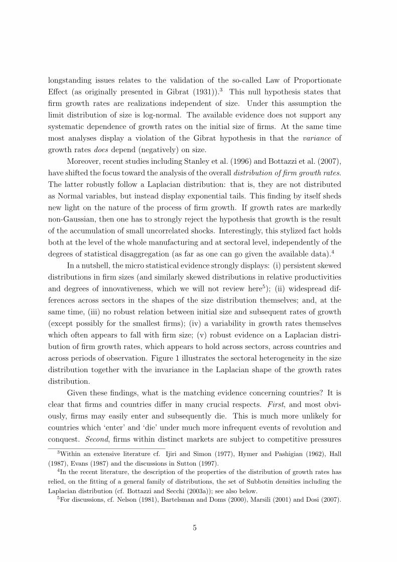
Moreover, recent studies including Stanley et al. (1996) and Bottazzi et al. (2007),

have shifted the focus toward the analysis of the overall distribution of firm growth rates.

The latter robustly follow a Laplacian distribution: that is, they are not distributed

as Normal variables, but instead display exponential tails. This finding by itself sheds

new light on the nature of the process of firm growth. If growth rates are markedly

non-Gaussian, then one has to strongly reject the hypothesis that growth is the result

of the accumulation of small uncorrelated shocks. Interestingly, this stylized fact holds

both at the level of the whole manufacturing and at sectoral level, independently of the

degrees of statistical disaggregation (as far as one can go given the available data).4

In a nutshell, the micro statistical evidence strongly displays: (i) persistent skewed

distributions in firm sizes (and similarly skewed distributions in relative productivities

and degrees of innovativeness, which we will not review here5); (ii) widespread dif-

ferences across sectors in the shapes of the size distribution themselves; and, at the

same time, (iii) no robust relation between initial size and subsequent rates of growth

(except possibly for the smallest firms); (iv) a variability in growth rates themselves

which often appears to fall with firm size; (v) robust evidence on a Laplacian distri-

bution of firm growth rates, which appears to hold across sectors, across countries and

across periods of observation. Figure 1 illustrates the sectoral heterogeneity in the size

distribution together with the invariance in the Laplacian shape of the growth rates

distribution.

Given these findings, what is the matching evidence concerning countries? It is

clear that firms and countries differ in many crucial respects. First, and most obvi-

ously, firms may easily enter and subsequently die. This is much more unlikely for

countries which ‘enter’ and ‘die’ under much more infrequent events of revolution and

conquest. Second, firms within distinct markets are subject to competitive pressures

3Within an extensive literature cf. Ijiri and Simon (1977), Hymer and Pashigian (1962), Hall

(1987), Evans (1987) and the discussions in Sutton (1997).4In the recent literature, the description of the properties of the distribution of growth rates has

relied, on the fitting of a general family of distributions, the set of Subbotin densities including the

Laplacian distribution (cf. Bottazzi and Secchi (2003a)); see also below.5For discussions, cf. Nelson (1981), Bartelsman and Doms (2000), Marsili (2001) and Dosi (2007).

5

0.001

0.01

0.1

1

-2 0 2 4 6 8 10 12 log(S)

log p (a) Food

0.01

0.1

1

-6 -4 -2 0 2 4 6

Food

(d)

0.001

0.01

0.1

1

-10 -5 0 5 10 15log(S)

log p (a) Chemicals

0.01

0.1

1

-6 -4 -2 0 2 4 6

Chemicals

(e)

0.001

0.01

0.1

1

-10 -5 0 5 10 15log(S)

log p (a) Machinery

0.01

0.1

1

-6 -4 -2 0 2 4 6

Machinery

(f)

Figure 1: Size distributions and growth rate distributions: evidence on US Manufac-

turing firms from Bottazzi and Secchi (2003b). Left plots show the kernel estimation of

the empirical density of the size distribution of firms in three illustrative industries (a),

while right plots show the corresponding fitted Subbotin density of the distribution of

growth rates (d-e-f). The industries are Food, Chemicals and Machinery and they are

simply selected for the sake of illustration.

6

that inevitably correlate with their performances. An increase in the size of one firm’s

market share in any particular market means the fall of other firms’ shares. As we

conjecture below, the very process of market competition is likely to contribute to the

observed statistical structure of firms’ growth rates. This is not necessarily the case

for countries as a whole. It trivially holds true that if some countries grow more than

others their share in world income will grow and vice versa. However, there is no

a priori reason to expect that country growth rates should yield statistical properties

similar to those displayed by micro-economic entities undergoing reciprocal competitive

pressures. Countries do not necessarily compete as firms do. In fact they might well co-

ordinate in order to achieve higher common rates of growth. With these qualifications

in mind, let us consider the macro, cross-country evidence.

3 The variables

We measure the per capita income of a country i in year t, say yit, by the country’s

per capita GDP at constant prices and constant exchange rates. The data source are

the Penn World Tables, version 6.1 (see Heston et al. (2002)) for 111 countries for

1960-1996.6

Let Yit be the aggregate income. This variable is a proxy for the actual ‘size’ of

a national economy. Another variable of interest is the level of economic development

of the various countries. This is primarily captured by the measure of per capita

income. Here we will consider both total and per capita GDP measures and compare

the empirical analyses using the two alternative variables.

To identify the country-specific properties of our variables over time, let us ‘de-

trend’ by “washing away” any component common to all countries in a given year. For

this purpose we consider ‘normalized’ (log) incomes defined by:

sit = log (yit) − log (yt)

Sit = log (Yit) − log (Yt)(1)

and calculate normalized year-by-year logarithmic growth rates as:

git = sit − si,t−1

Git = Sit − Si,t−1

(2)

We refer to these last variables as the growth shocks of interest.7 Notice that

6See the Appendix for details on the construction of our balanced panel.7The reader should be aware that we use the word ‘shock’ in tune with a common jargon of prac-

titioners of statistics: however, the terminology does not involve any commitment to the ‘exogeneity’

of the event itself. In fact, ‘shocks’ are endogenously generated by the very process of country growth.

7

Canning et al. (1998) only consider total GDP in their analysis of the distribution of

international growth rates, while we include here two different measures of national

income.

4 The distribution of levels of income

Let us start, somewhat symmetrically to the foregoing micro-evidence, from the distri-

butions of the levels of per capita incomes. An insightful new set of contributions has

recently been added to the empirics of international growth, shedding new light on the

statistical distributions of income levels and their change, if any, over time (see Quah

(1996, 1997), Durlauf and Quah (1999) Bianchi (1997), Jones (1997), Paap and van

Dijk (1998)). While it is not possible to discuss in any depth the secular evidence, no-

tice, first, that the mean per capita incomes have shown roughly exponential increases

since the “Industrial Revolution” in all countries that have been able to join it, and,

second, that the variance across countries has correspondingly exploded (more on this,

from different perspectives, in Bairoch (1981), Maddison (2001), Dosi, Freeman and

Fabiani (1994)). Given these long-term tendencies, the foregoing stream of analyses,

largely concerning the post World War II period, finds that the distribution of income

levels has been moving over the years to a bi-modal shape indicating a process of ‘polar-

ization’ of countries into two groups characterized by markedly different income levels.

Clearly this testifies against any prediction of a tendency towards global convergence

of all countries to a common income level.

Let us consider the time series available from Penn Tables version 6.1 and estimate

the kernel density for the distribution of normalized income and normalized per capita

income. Following the standard notation, the kernel density estimator for a sample of

data {xi}i=1:n is defined as:

f(x) =1

nh

n∑

i

K(x − xi

h) (3)

where K is the chosen kernel function and h the kernel bandwidth. This non-

parametric estimation procedure depends on the choice of the kernel bandwidth. The

larger the chosen bandwidth, the smoother the estimated density.

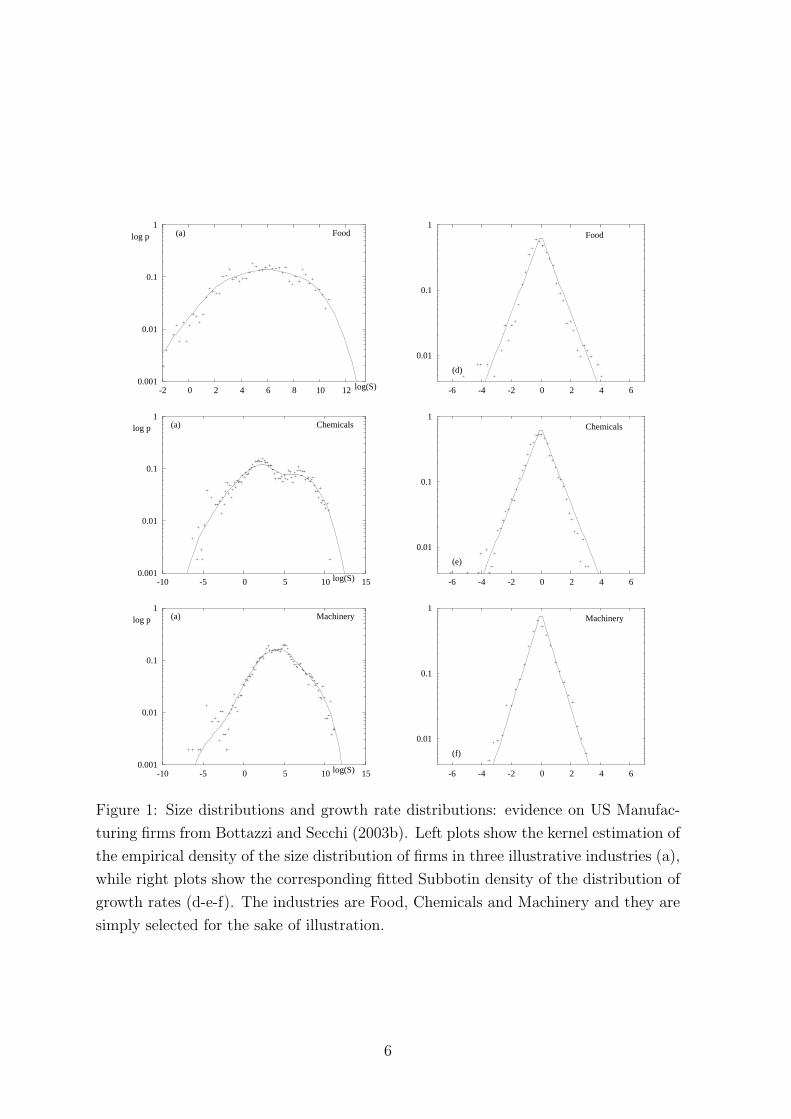
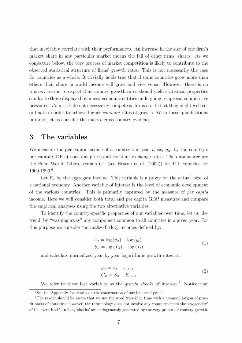
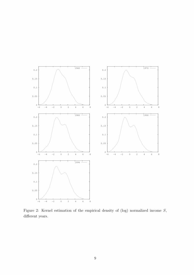
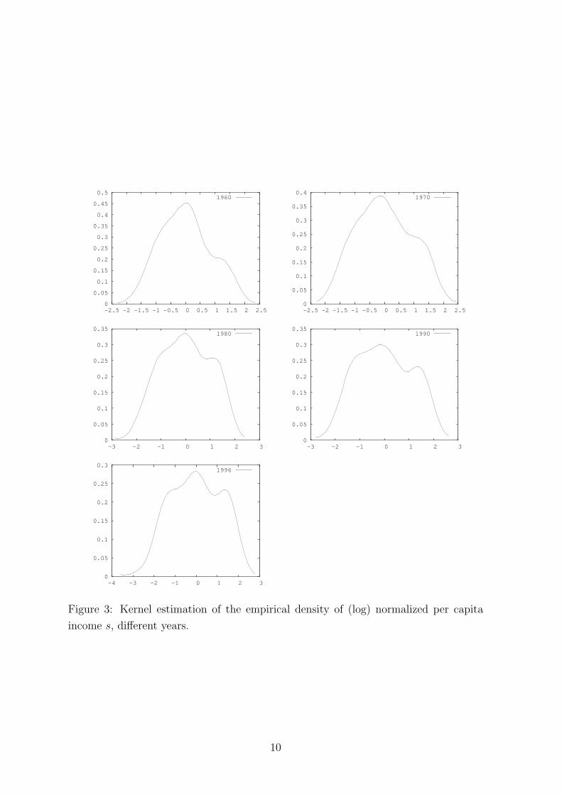
To get a graphical impression of the distributions, let us select a bandwidth with

the rule of thumb proposed in Silverman (1986). The exploratory plots in Figures 2

and 3 suggest that the estimated densities become less and less unimodal over the

years. The emergence of bimodality is more evident in the case of per capita income

than for total income. Figure 3 for per capita data shows that the distribution could

have been already bimodal in 1960 and that it might have gone towards a three-humps

8

0

0.05

0.1

0.15

0.2

-6 -4 -2 0 2 4 6 8

1960

0

0.05

0.1

0.15

0.2

-6 -4 -2 0 2 4 6 8

1970

0

0.05

0.1

0.15

0.2

-6 -4 -2 0 2 4 6 8

1980

0

0.05

0.1

0.15

0.2

-6 -4 -2 0 2 4 6 8

1990

0

0.05

0.1

0.15

0.2

-6 -4 -2 0 2 4 6 8

1996

Figure 2: Kernel estimation of the empirical density of (log) normalized income S,

different years.

9

0

0.05

0.1

0.15

0.2

0.25

0.3

0.35

0.4

0.45

0.5

-2.5 -2 -1.5 -1 -0.5 0 0.5 1 1.5 2 2.5

1960

0

0.05

0.1

0.15

0.2

0.25

0.3

0.35

0.4

-2.5 -2 -1.5 -1 -0.5 0 0.5 1 1.5 2 2.5

1970

0

0.05

0.1

0.15

0.2

0.25

0.3

0.35

-3 -2 -1 0 1 2 3

1980

0

0.05

0.1

0.15

0.2

0.25

0.3

0.35

-3 -2 -1 0 1 2 3

1990

0

0.05

0.1

0.15

0.2

0.25

0.3

-4 -3 -2 -1 0 1 2 3

1996

Figure 3: Kernel estimation of the empirical density of (log) normalized per capita

income s, different years.

10

shape after 1996. Formal multi-modality tests following the procedure introduced by

Silverman (1981) and first applied to income data by Bianchi (1997), confirm the

presence of bimodality starting from 1970.

Let us perform multi-modality tests on our longer time series. The Silverman test

is based on kernel estimation and relies on the calculation of critical kernel bandwidths

for the appearance of a given number of modes m. Call hc(m) the critical bandwidth

such that for any bandwidth h > hc(m) the density displays less than m modes, while

for any h < hc(m) the modes are at least m + 1. Any hc(m) may be used as a statistic

to test the hypothesis H0 : m modes vs H1 : more than m modes. The actual p-

value of the test can be calculated via bootstrapping. When pc(m) < α, where α

stands for the significance level of the test, one can reject the null hypothesis that the

distribution has m modes and not more. This test is known to have a bias towards

being conservative, in the sense that it leads to rejection in fewer cases than other tests

would. A procedure to correct this shortcoming has been proposed in Hall and York

(2001) for the unimodality test and it allows to calculate corrected actual p-values for

a given significance level of the test.8

Bianchi (1997) discusses some of the problems involved in using a fully non-

parametric technique. In particular he points out that this kind of test may fail to

detect multiple modes when modes are not well separated. For the particular instance

of GDP data, this may be the case when one considers logarithmic transformations of

the GDP data. The log transformation is a smoothed version of the actual data and

possible modes in the distribution will appear closer to each other than in the actual

data. To avoid this problem Bianchi suggests taking non-logarithmic transformations,

such as the per capita income relative to the sum of all incomes. Let us then define:

z∗i,t =yi,t∑yi,t

(4)

We report the outcome of our multi-modality Silverman tests on this specific

income measure to make our results comparable with Bianchi’s findings. Table 1 shows

estimates for selected years and for all years in the transition phase from unimodality

to a bimodality regime. We choose a significance of α = 0.1, a reasonable level for this

type of data. Scores that lead to rejection of the statistical hypothesis are highlighted

in italics. The results for the unimodality test include the Hall-York correction. We

confirm that the assumption of bimodality can not be rejected at a 10% level, even

since 1970.

8For a discussion on the advantages and the shortcomings of the Silverman test see Henderson et

al. (2007). The main shortcoming appears to be the fact that Silverman test is not nested and it may

thus yield inconclusive results.

11

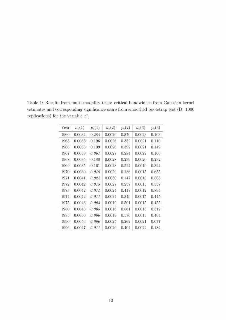
Table 1: Results from multi-modality tests: critical bandwidths from Gaussian kernel

estimates and corresponding significance score from smoothed bootstrap test (B=1000

replications) for the variable z∗.

Year hc(1) pc(1) hc(2) pc(2) hc(3) pc(3)

1960 0.0034 0.284 0.0026 0.370 0.0023 0.103

1965 0.0035 0.196 0.0026 0.352 0.0021 0.110

1966 0.0038 0.109 0.0026 0.392 0.0021 0.149

1967 0.0039 0.061 0.0027 0.284 0.0022 0.106

1968 0.0035 0.188 0.0028 0.239 0.0020 0.232

1969 0.0035 0.161 0.0023 0.524 0.0019 0.324

1970 0.0039 0.049 0.0029 0.186 0.0015 0.655

1971 0.0041 0.024 0.0030 0.147 0.0015 0.503

1972 0.0042 0.015 0.0027 0.257 0.0015 0.557

1973 0.0042 0.014 0.0024 0.417 0.0012 0.894

1974 0.0042 0.011 0.0024 0.349 0.0015 0.445

1975 0.0043 0.003 0.0019 0.501 0.0015 0.455

1980 0.0043 0.005 0.0016 0.861 0.0015 0.512

1985 0.0050 0.000 0.0018 0.576 0.0015 0.404

1990 0.0053 0.000 0.0025 0.262 0.0021 0.077

1996 0.0047 0.011 0.0026 0.404 0.0022 0.134

12

Henderson et al. (2007) also discuss an alternative test, the DIP test, and find

evidence for multi-modality since 1960. Their result indicates that the evidence on

multi-modality depends on the test used. Still, all evidence suggests that the last

decades have been characterized by multi-modality in international income levels, in-

dicating a process of ‘club convergence’ (Quah (1996)).

The results on bi-modality provide descriptive evidence that cannot be uncov-

ered from regression analysis, but does not shed any light on the determinants of the

cross-country distribution per se. Part of the interpretation involves the analysis of

the appropriate conditioning variables that might account for the emergence of sepa-

rate ‘clubs’ (Quah (1997)). Together, important circumstantial evidence is bound to

also come from the investigation of the statistical properties of growth rates. This is

discussed in the following section.

Even superficial comparisons between firm-level and country-level distributions

of ‘sizes’ (which should be properly understood as ‘total incomes of firms or countries’

and ‘per capita incomes’) reveal suggestive analogies concerning, at the very least, (i)

the skewness of distributions; (ii) the large width of their supports; and, (iii) high

persistence over time of relative rankings.

So far, the statistical properties of country growth rates have been much less

investigated (insightful exceptions include Canning et al. (1998), Lee et al. (1998)

and Maasoumi et al. (2007)). Indeed, such properties, and their possible analogies

with firm-level processes of growth are major topics to their own right which we shall

address below.

5 The statistical properties of growth shocks

5.1 Preliminary analysis

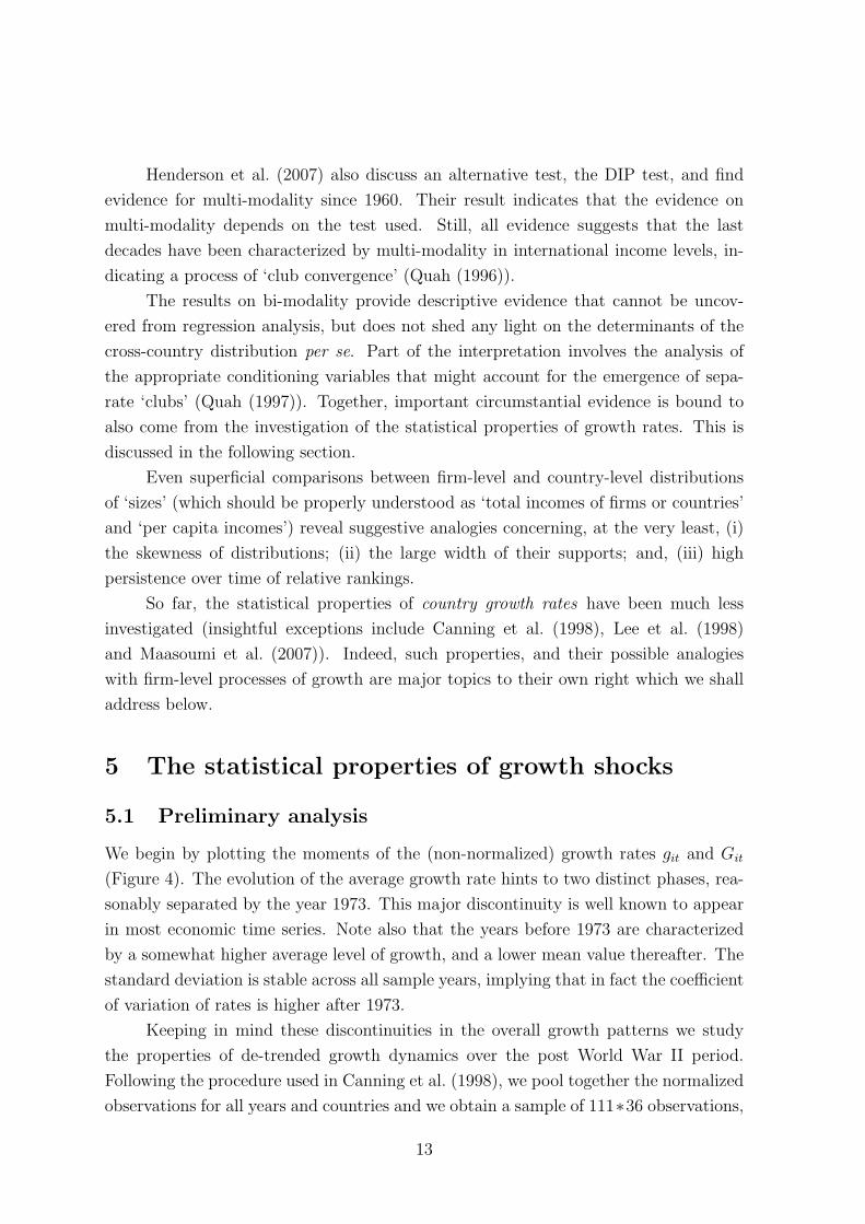
We begin by plotting the moments of the (non-normalized) growth rates git and Git

(Figure 4). The evolution of the average growth rate hints to two distinct phases, rea-

sonably separated by the year 1973. This major discontinuity is well known to appear

in most economic time series. Note also that the years before 1973 are characterized

by a somewhat higher average level of growth, and a lower mean value thereafter. The

standard deviation is stable across all sample years, implying that in fact the coefficient

of variation of rates is higher after 1973.

Keeping in mind these discontinuities in the overall growth patterns we study

the properties of de-trended growth dynamics over the post World War II period.

Following the procedure used in Canning et al. (1998), we pool together the normalized

observations for all years and countries and we obtain a sample of 111∗36 observations,

13

-0.02

-0.01

0

0.01

0.02

0.03

0.04

0.05

0.06

0.07

0.08

0.09

19961991198619811976197119661961

MeanStDev

0

0.01

0.02

0.03

0.04

0.05

0.06

0.07

0.08

0.09

19961991198619811976197119661961

MeanStDev

-5

0

5

10

15

20

25

19961991198619811976197119661961

SkewnessKurtosis

-5

0

5

10

15

20

25

19961991198619811976197119661961

SkewnessKurtosis

Figure 4: Evolution in time of the moments of the distribution of growth rates. Left

panels refer to git, right panels to Git.

large enough to support robust statistical analysis.

As a preliminary question let us ask whether higher or lower income countries

are characterized on average by (relatively) higher/lower growth rates.

We group countries into 40 equally populated subsets (‘bins’) according to income

s∗ (or S∗) and calculate the mean annual growth rate g∗ (or G∗) in each income

class. We fit a linear relation to the observations and account for heteroskedasticity

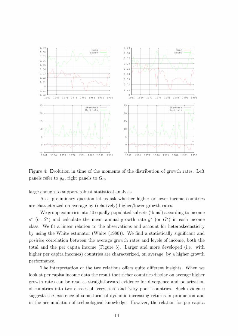
by using the White estimator (White (1980)). We find a statistically significant and

positive correlation between the average growth rates and levels of income, both the

total and the per capita income (Figure 5). Larger and more developed (i.e. with

higher per capita incomes) countries are characterized, on average, by a higher growth

performance.

The interpretation of the two relations offers quite different insights. When we

look at per capita income data the result that richer countries display on average higher

growth rates can be read as straightforward evidence for divergence and polarization

of countries into two classes of ‘very rich’ and ‘very poor’ countries. Such evidence

suggests the existence of some form of dynamic increasing returns in production and

in the accumulation of technological knowledge. However, the relation for per capita

14

-0.04

-0.03

-0.02

-0.01

0

0.01

0.02

0.03

-2 -1.5 -1 -0.5 0 0.5 1 1.5 2

per capita GDP

-0.015

-0.01

-0.005

0

0.005

0.01

0.015

0.02

-4 -3 -2 -1 0 1 2 3 4 5

total GDP

Mean(G)

Figure 5: The relation between average growth rate and income level for different

income classes. Linear fits are also shown. The left plot refers to per capita variables

(slope= 0.0113 ± 0.0012), the right one to total income ones (slope=0.0027 ± 0.0004).

resembles more a parable than a straight line: for the highest levels of per capita income

the relation is not significant or even becomes negative.

Conversely, the positive relation between average growth rate and total domestic

income hints at structural effects of the sheer size of an economy similar to ‘static’

economies of scale.9

5.2 The volatility of growth rates

Are higher income countries characterized by less volatile growth rates? Recent evi-

dence (see for example Pritchett (2000) and Fiaschi and Lavezzi (2005)) shows that the

volatility of growth rates is much higher for developing countries than for industrialized

ones. Throughout the process of development the levels of per capita GDP obviously

increase. Together, reductions in the dispersion of growth performance may also be

taken as an indication that countries move on more stable growth paths.

We again group countries by income, calculate the standard deviation of the

9It should be clear that the possible scale effects that we identify here do not necessarily bear

any direct relation with the scale effect that has been the object of controversy among ‘new growth’

theorists, as discussed in Jones (1999). One of the questionable predictions by the first wave of ‘new

growth’ models was the presence of a scale effect on the steady state growth according to which

an increase in the total population, and thus in the available specialized labor force, proportionally

increased the long run per capita growth. In some subsequent models the scale effect has shifted to

the level of per capita income, rather than its long run growth rate. In our strictly ‘inductive’ analysis

here we do not make any commitment to the existence of a steady state rate of growth: simply, the

statistical relations between income and growth appear to suggest some forms of increasing returns.

15

-3.8

-3.6

-3.4

-3.2

-3

-2.8

-2.6

-2.4

-2.2

-2 -1.5 -1 -0.5 0 0.5 1 1.5 2

log(StDev(g*))

Per capita Income (s*)

-3.8

-3.6

-3.4

-3.2

-3

-2.8

-2.6

-2.4

-2.2

-4 -3 -2 -1 0 1 2 3 4 5

log(StDev(G*))

Income (S*)

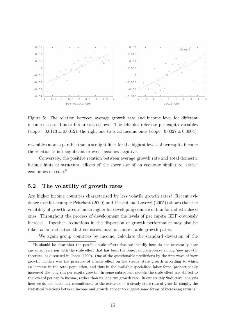
Figure 6: The relation between the logarithm of the volatility of growth rates and the

levels of income.

normalized growth shocks and associate this with the central value of income in each

class. Here, we uncover a negative relation between the log standard deviation of

growth rates and the level of per capita income. In other words the volatility of growth

rates scales with income as a power law.

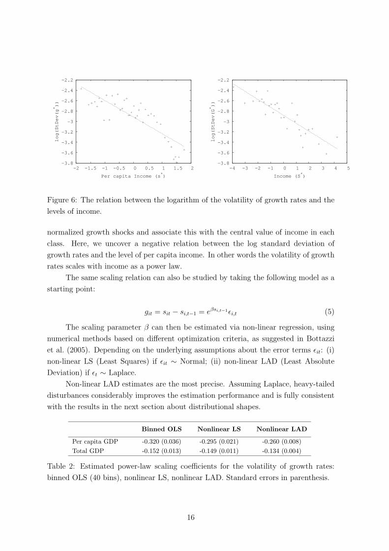
The same scaling relation can also be studied by taking the following model as a

starting point:

git = sit − si,t−1 = eβsi,t−1ǫi,t (5)

The scaling parameter β can then be estimated via non-linear regression, using

numerical methods based on different optimization criteria, as suggested in Bottazzi

et al. (2005). Depending on the underlying assumptions about the error terms ǫit: (i)

non-linear LS (Least Squares) if ǫit ∼ Normal; (ii) non-linear LAD (Least Absolute

Deviation) if ǫt ∼ Laplace.

Non-linear LAD estimates are the most precise. Assuming Laplace, heavy-tailed

disturbances considerably improves the estimation performance and is fully consistent

with the results in the next section about distributional shapes.

Binned OLS Nonlinear LS Nonlinear LAD

Per capita GDP -0.320 (0.036) -0.295 (0.021) -0.260 (0.008)

Total GDP -0.152 (0.013) -0.149 (0.011) -0.134 (0.004)

Table 2: Estimated power-law scaling coefficients for the volatility of growth rates:

binned OLS (40 bins), nonlinear LS, nonlinear LAD. Standard errors in parenthesis.

16

0.01

0.1

1

10

-0.4 -0.2 0 0.2 0.4

Low per capita GDPHigh per capita GDP

0.01

0.1

1

10

-0.4 -0.2 0 0.2 0.4

Small GDPLarge GDP

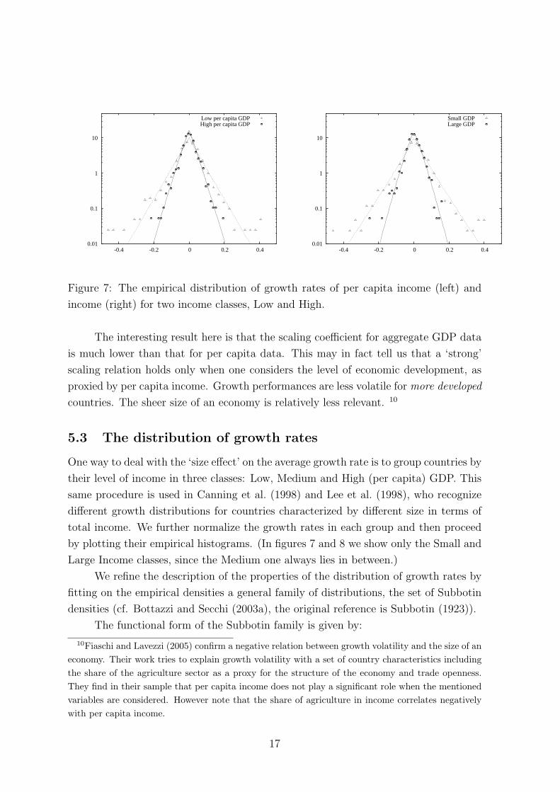
Figure 7: The empirical distribution of growth rates of per capita income (left) and

income (right) for two income classes, Low and High.

The interesting result here is that the scaling coefficient for aggregate GDP data

is much lower than that for per capita data. This may in fact tell us that a ‘strong’

scaling relation holds only when one considers the level of economic development, as

proxied by per capita income. Growth performances are less volatile for more developed

countries. The sheer size of an economy is relatively less relevant. 10

5.3 The distribution of growth rates

One way to deal with the ‘size effect’ on the average growth rate is to group countries by

their level of income in three classes: Low, Medium and High (per capita) GDP. This

same procedure is used in Canning et al. (1998) and Lee et al. (1998), who recognize

different growth distributions for countries characterized by different size in terms of

total income. We further normalize the growth rates in each group and then proceed

by plotting their empirical histograms. (In figures 7 and 8 we show only the Small and

Large Income classes, since the Medium one always lies in between.)

We refine the description of the properties of the distribution of growth rates by

fitting on the empirical densities a general family of distributions, the set of Subbotin

densities (cf. Bottazzi and Secchi (2003a), the original reference is Subbotin (1923)).

The functional form of the Subbotin family is given by:

10Fiaschi and Lavezzi (2005) confirm a negative relation between growth volatility and the size of an

economy. Their work tries to explain growth volatility with a set of country characteristics including

the share of the agriculture sector as a proxy for the structure of the economy and trade openness.

They find in their sample that per capita income does not play a significant role when the mentioned

variables are considered. However note that the share of agriculture in income correlates negatively

with per capita income.

17

0.01

0.1

1

10

100

-0.4 -0.3 -0.2 -0.1 0 0.1 0.2 0.3 0.4

Prob

(g)

g

High per capita GDPLow per capita GDP

0.01

0.1

1

10

100

-0.4 -0.3 -0.2 -0.1 0 0.1 0.2 0.3 0.4

Prob

(g)

g

Small GDPLarge GDP

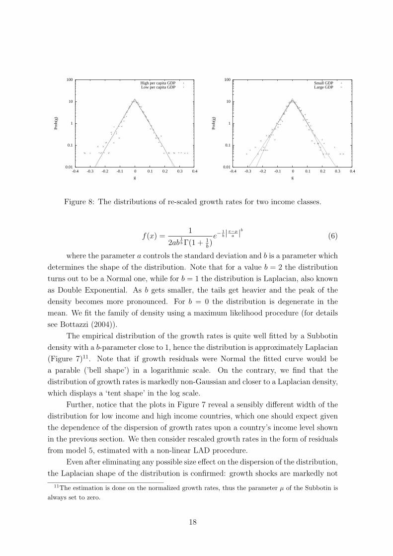
Figure 8: The distributions of re-scaled growth rates for two income classes.

f(x) =1

2ab1

b Γ(1 + 1

b)e−

1

b |x−µ

a |b

(6)

where the parameter a controls the standard deviation and b is a parameter which

determines the shape of the distribution. Note that for a value b = 2 the distribution

turns out to be a Normal one, while for b = 1 the distribution is Laplacian, also known

as Double Exponential. As b gets smaller, the tails get heavier and the peak of the

density becomes more pronounced. For b = 0 the distribution is degenerate in the

mean. We fit the family of density using a maximum likelihood procedure (for details

see Bottazzi (2004)).

The empirical distribution of the growth rates is quite well fitted by a Subbotin

density with a b-parameter close to 1, hence the distribution is approximately Laplacian

(Figure 7)11. Note that if growth residuals were Normal the fitted curve would be

a parable (’bell shape’) in a logarithmic scale. On the contrary, we find that the

distribution of growth rates is markedly non-Gaussian and closer to a Laplacian density,

which displays a ‘tent shape’ in the log scale.

Further, notice that the plots in Figure 7 reveal a sensibly different width of the

distribution for low income and high income countries, which one should expect given

the dependence of the dispersion of growth rates upon a country’s income level shown

in the previous section. We then consider rescaled growth rates in the form of residuals

from model 5, estimated with a non-linear LAD procedure.

Even after eliminating any possible size effect on the dispersion of the distribution,

the Laplacian shape of the distribution is confirmed: growth shocks are markedly not

11The estimation is done on the normalized growth rates, thus the parameter µ of the Subbotin is

always set to zero.

18

Rescaled

Growth rates growth rates

Income classes b a b a

Per capita GDP 0.9517 0.0407 1.0448 0.0411

(0.0277) (0.0008) (0.031) (0.0008)

Total GDP 0.9313 0.0398 1.0253 0.0402

(0.0269) (0.0008) (0.0310) (0.0008)

Low per capita GDP 0.9829 0.0498 1.0015 0.0376

(0.0498) (0.0017) (0.0510) (0.0013)

High per capita GDP 1.0644 0.0296 1.1845 0.0404

(0.0549) (0.0010) (0.0627) (0.0014)

Small GDP 0.9323 0.0503 0.9431 0.0384

(0.0467) (0.0018) (0.0474) (0.0014)

Large GDP 1.1885 0.0309 1.1845 0.0414

(0.0629) (0.0010) (0.0627) (0.0014)

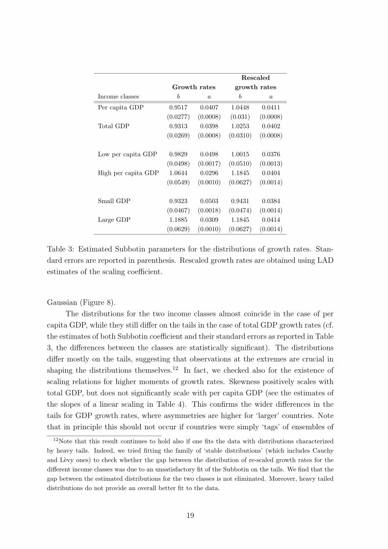
Table 3: Estimated Subbotin parameters for the distributions of growth rates. Stan-

dard errors are reported in parenthesis. Rescaled growth rates are obtained using LAD

estimates of the scaling coefficient.

Gaussian (Figure 8).

The distributions for the two income classes almost coincide in the case of per

capita GDP, while they still differ on the tails in the case of total GDP growth rates (cf.

the estimates of both Subbotin coefficient and their standard errors as reported in Table

3, the differences between the classes are statistically significant). The distributions

differ mostly on the tails, suggesting that observations at the extremes are crucial in

shaping the distributions themselves.12 In fact, we checked also for the existence of

scaling relations for higher moments of growth rates. Skewness positively scales with

total GDP, but does not significantly scale with per capita GDP (see the estimates of

the slopes of a linear scaling in Table 4). This confirms the wider differences in the

tails for GDP growth rates, where asymmetries are higher for ‘larger’ countries. Note

that in principle this should not occur if countries were simply ‘tags’ of ensembles of

12Note that this result continues to hold also if one fits the data with distributions characterized

by heavy tails. Indeed, we tried fitting the family of ‘stable distributions’ (which includes Cauchy

and Levy ones) to check whether the gap between the distribution of re-scaled growth rates for the

different income classes was due to an unsatisfactory fit of the Subbotin on the tails. We find that the

gap between the estimated distributions for the two classes is not eliminated. Moreover, heavy tailed

distributions do not provide an overall better fit to the data.

19

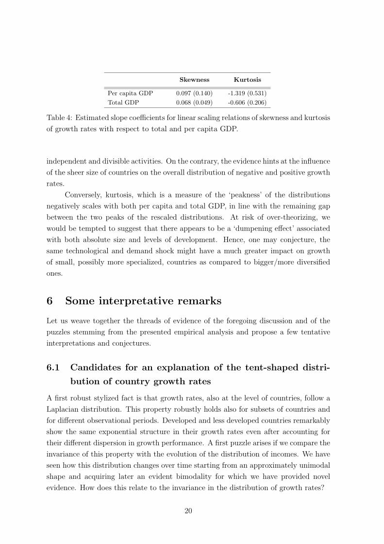
Skewness Kurtosis

Per capita GDP 0.097 (0.140) -1.319 (0.531)

Total GDP 0.068 (0.049) -0.606 (0.206)

Table 4: Estimated slope coefficients for linear scaling relations of skewness and kurtosis

of growth rates with respect to total and per capita GDP.

independent and divisible activities. On the contrary, the evidence hints at the influence

of the sheer size of countries on the overall distribution of negative and positive growth

rates.

Conversely, kurtosis, which is a measure of the ‘peakness’ of the distributions

negatively scales with both per capita and total GDP, in line with the remaining gap

between the two peaks of the rescaled distributions. At risk of over-theorizing, we

would be tempted to suggest that there appears to be a ‘dumpening effect’ associated

with both absolute size and levels of development. Hence, one may conjecture, the

same technological and demand shock might have a much greater impact on growth

of small, possibly more specialized, countries as compared to bigger/more diversified

ones.

6 Some interpretative remarks

Let us weave together the threads of evidence of the foregoing discussion and of the

puzzles stemming from the presented empirical analysis and propose a few tentative

interpretations and conjectures.

6.1 Candidates for an explanation of the tent-shaped distri-

bution of country growth rates

A first robust stylized fact is that growth rates, also at the level of countries, follow a

Laplacian distribution. This property robustly holds also for subsets of countries and

for different observational periods. Developed and less developed countries remarkably

show the same exponential structure in their growth rates even after accounting for

their different dispersion in growth performance. A first puzzle arises if we compare the

invariance of this property with the evolution of the distribution of incomes. We have

seen how this distribution changes over time starting from an approximately unimodal

shape and acquiring later an evident bimodality for which we have provided novel

evidence. How does this relate to the invariance in the distribution of growth rates?

20

Remarkably, the distributional invariance of GDP growth and per capita income

growth rates is a statistical feature analogous to that found with respect to corporate

growth rates. All the evidence robustly displays Laplacian distributions of growth

rates.

In the industrial organization literature, a common interpretation of the growth

process builds on a baseline stochastic model of growth of a given unit of observation

(e.g. a firm). If the growth process proceeded as the result of the cumulation in time

of independent growth shocks one would find the growth residuals g∗

it to be Normally

distributed and, thus, only representing ‘noise’. Instead, one finds quite structured

processes generating growth rates, which forces to reject the null hypothesis that growth

is simply the outcome of the sum of independent shocks. Thus, one has to search for

explanations of the growth process which admit that the ‘elementary’ growth shocks are

actually correlated with each other. And, indeed, such explanations ought to account

for the scale invariance of such property, since correlation mechanisms in the growth

process appear at all levels of observation, from firms to sectors to countries.13

This scale invariant regularity is thus in need of a convincing economic explana-

tion. Ultimately two diverse (but possibly complementary paths) seem to be available

for the modeler.

(i) A known statistical result refers to the property that a mixture of a small

number of Normal distributions produces fat-tailed distributions (see Lindsay (1995)).

Thus, a tent-shape distribution can be interpreted as a mixture of Normal distributions

given an appropriate parameterization. Mixtures are in principle an appealing tool for

understanding the tent-shape distribution of growth rates because one can envision mix-

tures of mixtures of mixtures, capturing different scales of observation. Also, one could

think of relating the components of the mixture to groups of countries representing

different convergence clubs (see Durlauf, Kourtellos and Minkin (2001)). Nevertheless,

a fundamental qualification should be considered. Such a statistical exercise, as well

as our ‘compact’ representation, both still demand an economic interpretation of the

underlying processes of growth yielding either the purported distributional mixtures

or, directly, a fat-tailed distributions of growth shocks.

(ii) A distinct interpretative strategy tries to explicitly interpret the observed

non-Normal distributions taking into account what we know about micro-processes of

growth, in particular acknowledging some basic correlating mechanisms in the processes

of market competition, together with the lumpiness of major competitive events. At

micro level, the exponential tails of the distribution of firm growth rates are explained

13On the sectoral evidence cf. Castaldi and Dosi (2004) and Castaldi and Sapio (2007). Both works

find evidence of exponential tails for the value added growth rates of sectors at 3-digit and 4-digit

level of aggregation.

21

in Bottazzi and Secchi (2006a) with a minimal probabilistic model which couples a

mechanism capturing some forms of increasing returns (more successful firms tend to

catch more business opportunities) together with competitive forces (firms compete for

market shares). In fact, we conjecture, fat-tailed distributions of growth rates might

turn out to be a quite generic property of a wide class of processes of industrial evolu-

tion. One could think of elaborating a similar multi-country model (keeping in mind

the different nature of inter-firm vs inter-country competition and complementarities).

A further challenge is to show how the observed structure of micro-shocks under-

lies similar macroscopic distributions. Recent research in macroeconomics has proposed

a few models where aggregate GDP fluctuations are explained by micro-shocks at firm

or sector level. In these models the micro-shocks aggregate in a non-trivial way: in-

stead of being diluted by the aggregation process, under certain circumstances they

amplify and form the basis for the structure of macro-shocks. In this vein, Gabaix

(2007) shows how a major part of aggregate growth shocks can be accounted for by

the growth of the top 100 firms in a country. Conversely, on the theory side, Bak

et al. (1993) and Durlauf (1994) model aggregate fluctuations as the outcome of the

propagation of demand shocks through inter-linked sectors.

From a different angle, Delli Gatti et al. (2005) also goes in the direction of

a micro-macro bridge, by relating the Double Exponential distribution of both firm

and country growth rates to the skewed distribution of firm size in a model based

on the interaction among heterogenous firms14. Quite overlapping evolutionary agent-

based models are also good candidates within this style of modeling (see Silverberg

and Verspagen (2005) for discussions of such a literature in a perspective pioneered

by Nelson and Winter (1982)). Indeed, preliminary exercises on the grounds of the

model in Dosi, Fagiolo and Roventini (2006), wherein macro-dynamics are nested into

heterogenous boundedly rational firms, show its ability to reproduce the tent-shape

distribution of firm and country growth rates.

6.2 Scaling of the growth volatility

The other stylized fact highlighted by our analysis is the existence of a negative relation

between the dispersion of growth rates and the level of per capita income. Moreover

the volatility scales with income as a power law. Its estimated coefficient for per capita

data, c = −0.32, is much higher than the e = −0.15 estimated with aggregate income

data. This seems to suggest that the ‘true’ scaling relation does not hold for size as

14The argument there, however, does not seem to be formally robust in so far as Gibrat-type

growth can be proved to be inconsistent with Laplace shocks and stationary Pareto size distributions,

see Bottazzi (2007).

22

such, as measured by the gross product of an economy, but it characterizes in primis the

level of development of a country. The structural effect of the total size of an economy

plays a role, but the stability of growth performances for high income countries stands

out more strongly when the income measure pertains to per capita incomes rather than

the sheer size of countries.

Amaral et al. (2001) and Lee et al. (1998) propose to interpret the scaling relation

by reference to a benchmark model of ‘complex organizations’. The idea is to view an

economic organization, i.e. a country in our specific instance, as made up of different

units of identical size. Then two opposite extreme scenarios may be contemplated. If

all units grew independently then the volatility of growth rates would fall as a power

law with coefficient −0.5 (a result of the law of large numbers, as suggested already

in Hymer and Pashigian (1962)). Conversely, if the composing units were perfectly

correlated there would be no relation between the volatility of growth shocks and size,

so we would find a slope of 0.

The estimated coefficients, lying in between 0 and −0.5 may be taken, in fact,

as an indicator of the overall ‘complexity’, or, better, the inner inter-relatedness of

the economic organization under study. If we translate this into our cross-country

analysis, we may take the negative relation between the volatility of growth rates and

the level of income as evidence of the importance of the internal interdependencies

of any national economy. Indeed, the patterns of income generation in a country via

input-output relations among the different sectors may be a candidate for explaining

the degree of ‘internal correlation’ which produces the observed stylized fact. Scaling

relations clearly depend also on the number of activities (or “lines of business”) within

the entity under consideration (e.g. a country or a firm). Keeping this in mind, a

possible explanation for the different observed scaling slopes could be the following.

Economic development is likely to be correlated with the density of economic activities

or, putting it another way, with the number of different economic sectors in which a

country is active in. Hence, in line with the evidence, richer countries, characterized

by a higher number of relevant economic activities, would display less variable growth

rates, while poorer countries embodying fewer activities would be more volatile in their

growth performances.15 Yet another analogy can be made here with the micro level:

as Bottazzi et al. (2001) find, the standard deviation of growth rates declines with the

number of sub-markets where firms operate.16

15Along these lines, see also Harberger (1998) for some insights.16See also Bottazzi and Secchi (2006b) for a branching model of corporate diversification able to

account for such an evidence.

23

7 Conclusions

The evidence presented in this work suggests striking invariances in the processes of

growth that hold at different levels of observation, from firms to whole countries. This

work has discussed new statistical results on output growth rates that are in line with

what has been found in the recent literature on firm growth rates. The scaling relations

analyzed in this work concerned both to the average and the dispersion of growth rates.

A caveat to keep in mind when dealing with such scaling laws, as Brock (1999) suggests,

is that, “Most of them are ‘unconditional objects’, i.e. they only give properties of

stationary distributions, e.g. ‘invariant measures’, and hence cannot say much about

the dynamics of the stochastic process which generated them. ... Nevertheless, if a

robust scaling law appears in data, this does restrict the acceptable class of conditional

predictive distributions somewhat.” (p.426).

The common exponential properties of growth rates mark widespread correlat-

ing mechanisms which aggregation does not dilute. A puzzling question relates to

the nature of such mechanisms that might well be different across levels. For exam-

ple, one may reasonably conjecture that at micro level ‘lumpy’ technological events,

idiosyncratic increasing returns, together with the inter-dependences induced by the

very competitive process, may robustly account for the ‘tent-shape’ distribution of

growth shocks. Conversely, at country level, it might well be due to, again, some forms

of increasing returns together with the inter-sectoral propagation of technological and

demand impulses.

In any case, both micro and macro evidence supports the impressionistic Schum-

peterian intuition that growth is not a smooth process but rather tends to proceed by

“fits and starts”. Granted that, the big ensuing challenge is to better understand why

and how this is so.

One way to disentangle the underlying mechanisms involves, as Brock (1999)

suggests, the joint consideration of scaling laws with other types of statistical evi-

dence that may provide conditioning schemes useful to refine the evidence on the data

generating process. Maasoumi et al. (2007) propose a new way of conditioning using

non-parametric models that can be applied in a flexible way to growth data. We also

expect that precious insights are likely to come by linking the evidence on growth with

the processes of arrival of technological and organizational innovations.

The theorist faces symmetric challenges.

One of them regards the relationships between the properties of the distributions

of growth rates - which appear to be robustly exponential, irrespectively of the time

and the scale of observation,- and the distributions of the levels (for example, the size

of firms, countries or per capita GDP), whose shapes appear to be much more time-

24

and scale-specific. In this respect, a delicate, still largely unresolved, issue concerns the

points of relative strength and weakness of two distinct heuristic strategies, namely,

a first one attempting to derive the observed statistical properties from mixtures of

underlying normally distributed variables, and, a second one focusing on the identifi-

cation of possible generating processes which might directly yield the observed sample

paths.

Another, related, challenge, concerns the ability of the models to account, at the

same time, for both microscopic and macroscopic patterns of growth. Ultimately the

emerging evidence on such patterns, some of which has been discussed in this work,

ought to be an important yardstick to evaluate the robustness and success of different

theoretical efforts aimed at modeling the growth dynamics of contemporary economies.

Appendix

The country variables used in the analysis are taken from the most recent version of the

Penn World Tables (Heston et al. (2002)). Version 6.1 extends the previous Version 5.6

by providing data until 1998 for most countries. The benchmark year has been changed

from 1985 to 1996. We choose to perform our analysis on a balanced panel of 111

countries whose variables of interest are available for all years between 1960 and 1996.

The most notable exclusions of countries from the database are for entities that have

undergone some political transformation affecting the definition of their own borders,

such as Germany and former-USSR. Nevertheless, the remaining sample appears to

be quite representative. Table A.1 provides a list of the 111 countries included in the

balanced panel.

25

Table A.1: List of countries included in our balanced panel.

Code Country Code Country Code Country

AGO Angola GBR United Kingdom NER Niger

ARG Argentina GHA Ghana NGA Nigeria

AUS Australia GIN Guinea NIC Nicaragua

AUT Austria GMB Gambia, The NLD Netherlands

BDI Burundi GNB Guinea-Bissau NOR Norway

BEL Belgium GNQ Equatorial Guinea NPL Nepal

BEN Benin GRC Greece NZL New Zealand

BFA Burkina Faso GTM Guatemala PAK Pakistan

BGD Bangladesh GUY Guyana PAN Panama

BOL Bolivia HKG Hong Kong PER Peru

BRA Brazil HND Honduras PHL Philippines

BRB Barbados HTI Haiti PNG Papua New Guinea

BWA Botswana IDN Indonesia PRT Portugal

CAF Central African Rep. IND India PRY Paraguay

CAN Canada IRL Ireland ROM Romania

CHE Switzerland IRN Iran RWA Rwanda

CHL Chile ISL Iceland SEN Senegal

CHN China ISR Israel SGP Singapore

CIV Cote d’Ivoire ITA Italy SLV El Salvador

CMR Cameroon JAM Jamaica SWE Sweden

COG Congo, Rep. of JOR Jordan SYC Seychelles

COL Colombia JPN Japan SYR Syria

COM Comoros KEN Kenya TCD Chad

CPV Cape Verde KOR Korea, Rep. of TGO Togo

CRI Costa Rica LKA Sri Lanka THA Thailand

CYP Cyprus LSO Lesotho TTO Trinidad Tobago

DNK Denmark LUX Luxembourg TUR Turkey

DOM Dominican Rep. MAR Morocco TWN Taiwan

DZA Algeria MDG Madagascar TZA Tanzania

ECU Ecuador MEX Mexico UGA Uganda

EGY Egypt MLI Mali URY Uruguay

ESP Spain MOZ Mozambique USA USA

ETH Ethiopia MRT Mauritania VEN Venezuela

FIN Finland MUS Mauritius ZAF South Africa

FJI Fiji MWI Malawi ZAR Congo, Dem. Rep.

FRA France MYS Malaysia ZMB Zambia

GAB Gabon NAM Namibia ZWE Zimbabwe

26

References

Amaral, L.A.N., P. Gopikrishnan, V. Plerou, and H. E. Stanley (2001), A model for

the growth dynamics of economic organizations, Physica A, 299, pp.127-136.

Bairoch, P. (1981), The main trends in national economic disparities since the indus-

trial revolution in P. Bairoch and M. Levy-Leboyer, eds. Disparities in Economic

Development since the Industrial Revolution, Oxford: Macmillan.

Bak, P., K. Chen, J. Scheinkman and M. Woodford (1993), Aggregate fluctuations from

independent Sectoral Shocks: Self-Organized Criticality in a Model of Production

and Inventory Dynamics, Ricerche Economiche, 47, pp.3-30.

Bartelsman, E.J. and M. Doms (2000), Understanding Productivity: Lessons from

Longitudinal Microdata, Journal of Economic Literature, 38, pp.569-594.

Bianchi, M. (1997), Testing for convergence: Evidence from nonparametric multimodal-

ity tests, Journal of Applied Econometrics, 12, pp.393-409.

Bottazzi, G. (2004), Subbotools user’s manual, available on line at

http://cafim.sssup.it/∼giulio/software/subbotools/doc/subbotools.pdf.

Bottazzi, G. (2007), On the Irreconciliability of Pareto and Gibrat Laws, LEM Working

Paper 2007-10, Sant’Anna School of Advanced Studies, Pisa, Italy.

Bottazzi, G., E. Cefis, G. Dosi and A. Secchi (2007), Invariances and Diversities in the

Evolution of Manufacturing Industries, Small Business Economics, forthcoming

Bottazzi, G., G. Dosi, M. Lippi, F. Pammolli and M. Riccaboni (2001), Innovation and

Corporate Growth in the Evolution of the Drug Industry, International Journal of

Industrial Organization, 19, pp.1161-1187.

Bottazzi, G., Coad, A., Jacoby, N. and A. Secchi (2006), Corporate growth and indus-

trial dynamics: evidence from French manufacturing, LEM Working Paper, Sant’

Anna School, Pisa.

Bottazzi, G. and A. Secchi (2003a), Why are distributions of firm growth rates tent-

shaped?, Economics Letters, 80, pp.415-420.

Bottazzi, G. and A. Secchi (2003b), Common Properties and Sectoral Specificities in

the Dynamics of US Manufacturing Companies, Review of Industrial Organization,

23, pp.217-232.

27

Bottazzi, G. and A. Secchi (2006), Explaining the Distribution of Firms Growth Rates,

Rand Journal of Economics, 37, pp.234-263.

Bottazzi, G. and A. Secchi (2006b), Gibrat’s Law and Diversification, Industrial and

Corporate Change, pp. 847-875.

Brock, W.A. (1999), Scaling in Economics: a Reader’s Guide, Industrial and Corporate

Change, 8, pp.409-446.

Canning, D., L. A. N. Amaral, Y. Lee, M. Meyer and H. E. Stanley (1998), Scaling the

volatility of GDP growth rates, Economics Letters, 60, pp.335-341.

Castaldi, C. and G. Dosi (2004), Income levels and income growth: Some new cross-

country evidence and some interpretative puzzles, LEM Working Paper 2004-18,

Sant’Anna School of Advanced Studies, Pisa.

Castaldi, C. and S. Sapio (2007), Growing like Mushrooms? Sectoral Evidence from

Four Large European Economies, GGDC Working Paper, University of Groningen,

the Netherlands, forthcoming in Journal of Evolutionary Economics.

Delli Gatti, D., C. Di Guilmi, E. Gaffeo, G. Giulioni, M. Gallegati and A. Palestrini

(2005), A new approach to business fluctuations: heterogenous interacting agents,

scaling laws and financial fragility, Journal of Economic Behaviour and Organization,

56, pp.489-512.

Dosi, G. (2007), Statistical Regularities in the Evolution of Industries. A Guide through

some Evidence and Challenges for the Theory, in S. Brusoni and F. Malerba (eds.),

Perspectives on Innovation, Cambrige University Press.

Dosi, G., G. Fagiolo and A. Roventini (2006), An Evolutionary Model of Endogenous

Business Cycles, Computational Economics, 27, pp.3-34.

Dosi, G., Freeman, C. and Fabiani, S. (1994), The process of economic development:

introducing some stylized facts and theories on technologies, firms and institutions,

Industrial and Corporate Change, 3, pp.1-45.

Dosi, G., O. Marsili, L. Orsenigo and R. Salvatore (1995), Learning, Market Selection

and the Evolution of Industrial Structures, Small Business Economics, 7, pp.1-26.

Durlauf, S.N. and D. Quah (1999), The New Empirics of Economic Growth, in J.B.

Taylor and M. Woodford (eds.), Handbook of Macroeconomics, vol. 1A, North Hol-

land Elsevier Science .

28

Durlauf, S.N., A. Kourtellos and A. Minkin (2001), The Local Solow Growth Model,

European Economic Review, 45, pp.928-940.

Durlauf, S.N. (1994), Path Dependence in Aggregate Output, Industrial and Corporate

Change, 3, pp.149-171.

Evans, D.S. (1987), The Relationship between Firm Size, Growth and Age: Estimates

for 100 Manufacturing Industries, Journal of Industrial Economics, 35, pp.567-581.

Fagiolo, G., Napoletano, M. and Roventini, A. (2007), Are output growth-rate distri-

butions fat-tailed? Some evidence from OECD countries, Journal of Applied Econo-

metrics, forthcoming.

Fiaschi, D. and A.M. Lavezzi (2005), On the determinants of growth volatility: a non-

parametric approach, Working paper, University of Pisa.

Gabaix, X. (2007), The Granular Origins of Aggregate Fluctuations, Working Paper,

MIT.

Gibrat, R. (1931), Les inegalites economiques, Paris: Librairie du Recueil Sirey.

Goerlich Gisbert, F.J. (2003), Weighted samples, kernel density estimators and con-

vergence, Empirical Economics, 28, pp.335-351.

Hall, B.H. (1987), The Relationship between Firm Size and Firm Growth in the US

Manufacturing Sector, Journal of Industrial Economics, 35, pp.583-606.

Hall, P. and York, M. (2001), On the Calibration of Silverman’s Test for Multimodality,

Statistica Sinica, 11, pp.515-536.

Harberger, A.C. (1998), A Vision of the Growth Process, American Economic Review,

88. pp.1-32.

Hart, P.E. and S.J. Prais (1956), The Analysis of Business Concentration, Journal of

the Royal Statistical Society 119, pp.150-191.

Henderson, D.J., C. F. Parmeter and R. R. Russell (2007), Convergence clubs: Evidence

from Calibrated Modality Tests, working paper, University of California, Riverside,

forthcoming in Journal of Applied Econometrics.

Heston, A., R. Summers and B. Aten (2002), Penn World Table Version 6.1, Center

for International Comparisons at the University of Pennsylvania (CICUP), October

2002.

29

Hymer, S. and P. Pashigian (1962), Firm Size and Rate of Growth, Journal of Political

Economy, 70, pp.556-569.

Ijiri, Y. and H.A. Simon (1977), Skew Distributions and the Size of Business Firms,

Amsterdam: North Holland.

Jones, C.I. (1997), On the evolution of the world income distribution, Journal of Eco-

nomic Perspectives, 11, pp.19-36.

Jones, C.I. (1999), Growth: with or without scale effects?, American Economic Review,

Papers and Proceedings, 89, pp.139-144.

Lee, Y., L. A. N. Amaral, D. Canning, M. Meyer and H. E. Stanley (1998), Universal

Features in the Growth Dynamics of Complex Organizations, Phys. Rev. Lett., 81,

pp.3275-3278.

Lindsay, B.G. (1995), Mixture Models: Theory, Geometry and Applications, Hayward,

CA: Institute for Mathematical Statistics.

Maasoumi, E., J. Racine and T. Stengos (2007), Growth and convergence: A profile of

distribution dynamics and mobility, Journal of Econometrics, 136, pp.483-508.

Maddison, A. (2001), The World Economy: a Millennial Perspective, Paris: OECD.

Marsili, O. (2001), The Anatomy and Evolution of Industries, Cheltenham, UK: Ed-

ward Elgar.

Nelson, R.R. (1981), Research on Productivity Growth and Productivity Differences:

Dead Ends and New Departures, Journal of Economic Literature, 19, pp.1029-64.

Nelson, R.R. and S.G. Winter (1982), An Evolutionary Theory of Economic Change,

Cambridge, MA: Harvard University Press.

Paap, R. and H. K. van Dijk (1998), Distribution and mobility of wealth of nations,

European Economic Review, 42, 1269-1293.

Pritchett, L. (2000), Understanding Patterns of Economic Growth: Searching for Hills

among Plateaus, Mountains and Plains, The World Bank Economic Review, 105,

pp.221-250.

Quah, D. (1996), Twin peaks: growth and convergence in models of distribution dy-

namics, Economic Journal, 106, pp.1045-1055.

30

Quah, D. (1997), Empirics for growth and distribution: stratification, polarization and

convergence clubs, Journal of Economic Growth, 2, pp.27-59.

Silverman, B. W. (1981), Using Kernel Density Estimates to investigate Multi-

modality, Journal of the Royal Statistical Society, B, 43, pp.97-99.

Silverman, B. W. (1986), Density Estimation for Statistics and Data Analysis, London:

Chapman and Hall.

Silverberg, G. and B. Verspagen (2005), Evolutionary theorizing on economic growth,

in Dopfer, K, ed. (2005) The Evolutionary Principles of Economics, Cambridge:

Cambridge University Press.

Simon, H. A. and C. P. Bonini (1958), The Size Distribution of Business Firms, Amer-

ican Economic Review, 48, pp.607-617.

Stanley, M. H. R., L. A. N. Amaral, S. V. Buldyrev, S. Havlin, H. Leschhorn, P.

Maass, M. A. Salinger and H. E. Stanley (1996), Scaling Behavior in the Growth of

Companies, Nature, 379, pp.804-806.

Steindl, J. (1965), Random Processes and the Growth of Firms, London: Griffin.

Subbotin, M. (1923), On the law of frequency of errors, Matematicheskii Sbornik, 31,

pp.296-301.

Sutton, J. (1997), Gibrat’s Legacy, Journal of Economic Literature, 35, pp.40-59.

Temple, J. (1999), The New Growth Evidence, Journal of Economic Literature, 37,

pp.112-156.

White, H.A. (1980), A heteroskedasticity-consistent covariance matrix estimator and

a direct test for heteroskedasticity, Econometrica, 48, pp.817-838.

31