The pentagram map on Grassmannians

Raul Felipe ∗

CIMATGuanajuato, Mexico

Gloria Marı Beffa †

Mathematics DepartmentUniversity of Wisconsin - Madison

July 16, 2015

Abstract

In this paper we define a generalization of the pentagram map to a map ontwisted polygons in the Grassmannian space Gr(n,mn). We define invariants ofGrassmannian twisted polygons under the natural action of SL(nm), invariantsthat define coordinates in the moduli space of twisted polygons. We then provethat when written in terms of the moduli space coordinates, the pentagram mapis preserved by a certain scaling. The scaling is then used to construct a Laxrepresentation for the map that can be used for integration.

1 Introduction

In the last five years there has been a lot of activity around the study of the pentagrammap, its generalizations and some related maps. The map was originally defined byRichard Schwartz over two decades ago ([10]) and after a dormant period it came backwith the publication of [8], where the authors proved that the map, when defined ontwisted polygons, was completely integrable. The literature on the subject is quitesizable by now, as different authors proved that the original map on closed polygonswas also completely integrable ([9], [13]); worked on generalizations to polygons inhigher dimensions and their integrability ([1], [2], [5], [6]); and studied the integrabilityof other related maps ([11], [7]). The subject has also branched into geometry andcombinatorics, this bibliography refers only to some geometric generalizations of themap and is by no means exhaustive.

The success of the map is perhaps due to its simplicity. The original map isdefined on closed convex polygons in RP2. The map takes a convex polygon in theprojective plane to the one formed by the intersection of the lines that join every othervertex, as in the figure. The mathematical consequences of such a simple constructionare astonishing (in particular, the pentagram map is a double discretization of theBoussinesq equation, a well-known completely integrable system modeling waves, see[8]). Integrability is studied not for the map itself, but for the map induced by it onthe moduli space of planar projective polygons, that is on the space of equivalenceclasses of polygons up to a projective transformation. In [8] the authors defined it ontwisted polygons, or polygons with a monodromy after a periodN , and proved that themap induced on the moduli space is completely integrable. (The map is equivariant

∗raulf@cimat.mx†maribeff@math.wisc.edu; Corresponding author

1

under projective transformations, thus the existence of the moduli induced map isguaranteed.)

In this paper we look at the generalization of the map from the Grassmannianpoint of view. If we think of RP2 as the Grassmaniann Gr(1, 3), that is, the space ofhomogeneous lines in R3, then the polygon would be a polygon in the Grassmannianunder the usual action of SL(2 + 1), with each side representing a homogeneous planeas in the picture. The case of RPm−1 was studied in [1] where the authors proved thatthe generalized pentagram map was integrable for low dimensions, and conjecturedthat a scaling existed for the map that ensured the existence of a Lax pair and itsintegrability. The conjecture was proved in [6]. We can also consider this case asGr(1,m), m ≥ 3. From this point of view, it is natural to investigate the generalizedmap defined on polygons in Gr(n,mn), where m and n are positive integers, m ≥ 3.In this paper we define and study the generalization of the pentagram map to twistedGrassmannian polygons in Gr(n,mn), m ≥ 3.

Figure 1: the pentagram map on pentagons in Gr(1, 3)

The first step is to define the map on the moduli space of Grassmannian twistedpolygons, that is, on the space of equivalence classes of Grassmannian twisted poly-gons, under the classical action of SL((m − 1)n + n) that generalizes the projectiveaction of PSL(m) on RPm−1. We do that by carefully studying the moduli space andfinding generic coordinates that can be used to write the map in a convenient way(as in the case of the original pentagram map, the map can only be defined generi-cally). The coordinates are found with the use of a discrete moving frame constructedthrough a normalization process similar to the one described in [4]. The classificationof invariants under this action is, as far as we know, unknown, and it is completed insection 3.

In section 4 we study the case m = 2s. In a parallel fashion to the study in [6], weproceed to write the pentagram map on the moduli space in the chosen coordinates,and we show that it can be written as the solution of a linear system of equations.We use that description and Cramer’s rule to prove that the map is invariant undera certain scaling. As it was the case in [6], a critical part of the study is a fundamen-tal lemma that decomposes the coefficient matrix of the system into terms that arehomogeneous with respect to the scaling. This is lemma 4 for the even dimensionalcase, and lemma 9 for the odd dimensional one. The proofs of the rest of the resultsare supported by those two lemmas. Once the invariance under scaling is proved, theconstruction of a Lax representation is immediate when we introduce the scaling intoa natural parameter-free Lax representation that exists for any map induced on themoduli space by a map on polygons.

In section 5 we prove the case m = 2s+ 1.

2

2 Definitions and notations

Let Gr(p, q) be the set of all p-dimensional subspaces of V = Rq or V = Cq. Eachl ∈ Gr(p, q) can be represented by a matrix Xl of size q×p such that the columns forma basis for l. We denote this relation by l =< Xl >. Clearly l =< Xl >=< Xld > forany d ∈ GL(p), and the representation is not unique. Hence, Gr(p, q) can be viewedas the space of equivalence classes of q×p matrices, where two matrices are equivalentif their columns generate the same subspace. An element of this class, Xl is called alift of l. The name reflects Gr(p, q) admitting the structure of a homogeneous spaceof dimension p(q− p). Indeed, consider the Lie group SL(q+ p), represented by blockmatrices of the form (

Aq−p×q−p Bq−p×pCp×q−p Ep×p

).

Let H be the subspace defined by Bq−p×p = 0. One can show that SL((q− p) + p)/His isomorphic to Gr(p, q) and the natural action of SL((q− p) + p) on Gr(p, q) is givenby

g· < X >=< gX > .

Consider Gr(n,mn) for any positive integers n,m, and let SL((m − 1)n + n) ×Gr(n,mn) −→ Gr(n,mn) be the natural action of the group SL(mn) on Gr(n,mn).

A twisted N -gon in Gr(n,mn) is a map φ : Z −→ Gr(n,mn) such that φ(k+N) =M · φ(k) for all k ∈ Z and for some M ∈ SL(mn). The matrix M is called themonodromy of the polygon and N is the period. We will also denote an N -gon by℘ = (lk), where lk = φ(k).

Let X = (Xk) be an arbitrary lift for an N -gon ℘ = (lk) with monodromy M , andchoose X so it is also twisted, that is, XN+k = MXk for all k. For any discrete closedN -polygon d = (dk) in GL(n) (i.e. satisfying dk+N = dk), we have that Xd = (Xkdk)is also a lift for the same polygon, with the same monodromy M .

Let us denote by PN the moduli space of twisted N -gons in Gr(n,mn), thatis, the space of equivalence classes of twisted polygons under the natural action ofSL(mn). We will also denote by PlN the moduli space of N -gons in Rmn×n (orCmn×n, wherever the lifts live), under the linear action of SL(mn).

AN -gon ℘ = (lk) is called regular if the matrix ρk = (Xk Xk+1 . . . Xk+m−2 Xk+m−1)satisfies the following condition

det ρk = |(Xk Xk+1 . . . Xk+m−2 Xk+m−1)| 6= 0, (1)

for any k ∈ Z and any lift X (clearly, it suffices to check the condition for oneparticular lift). In other words, the columns of the matrix constitute a basis of Rmn(or Cmn) for all k ∈ Z.

3 The moduli space of twisted polygons in Gr(n,mn)

In this section we will prove that the moduli space of regular twisted polygons, PN ,is a N(m− 1)n-dimensional manifold and will define local coordinates.

Assume ℘ = (lk), lk ∈ Gr(n,mn) is a regular twisted N -gon and let Xk beany twisted lift. By dimension counting, and given that ℘ is regular, for any k =0, . . . , N − 1 we can find n× n matrices aik, i = 0, . . . ,m− 1 such that

Xk+m = Xm+k−1am−1k + · · ·+Xk+1a

1k +Xka

0k. (2)

Notice that if ρk is as in (1), then

ρk+1 = ρk

On On . . . On a0kIn On . . . On a1k...

. . .. . .

......

On . . . In On am−2k

On . . . On In am−1k

= ρkQk, (3)

3

where Qk is the matrix above. Using (1), this implies that det a0k 6= 0, for all k.Notice that ρN = ρ0Q0Q1, . . . , QN−1. Thus, if ρ0 = I, the monodromy is givenby M = Q0 . . . QN−1, and for other choices M = ρ0Q0 . . . QN−1ρ

−10 . Thus, only

the conjugation class of monodromy of the system defined by the matrices Qk, k =0, . . . , N − 1, is well-defined, not the monodromy itself.

Theorem 1. Assume m and N are coprime. Then, for any regular twisted N -gon,℘, there exists a lift V = (Vk) such that

det(Vk, Vk+1, . . . , Vk+m−1) = 1, (4)

for any k = 0, . . . , N − 1, and such that if aik are given as in (2), then

1.a0k = diagonal(r1k, . . . , r

sk),

where each rsk is an upper triangular Toeplitz matrix with det a0k = 1.

2. We can choose V such that all am−1k ’s entries, for any k, are generated by

N(n2 − n+ 1) independent functions.

The remaining N(n−1)m entries of aik, i 6= 0,m−1, together with those above, definea coordinate system on PN .

Proof. Let X = (Xk) be any twisted lift of the twisted polygon ℘. We will callVk = Xkdk and show that we can find a closed polygon in GL(n), dk, such that theconditions of the theorem are satisfied. If Vk = Xkdk we have

(Vk, . . . , Vk+m−1) = (Xk, . . . , Xk+m−1)diag(dk, dk+1, . . . , dk+m−1). (5)

First of all we will show that condition (4) determines the values of δk = det dk, forany k. Indeed, from (5) we have that

k+m−1∏i=k

δi = Zk,

where Zk = det(Xk, . . . , Xk+m−1)−1 is determined by the choice of lift. These equa-tions determine δk uniquely whenever N and m are coprime, as shown in [6]. Let uscall bik the invariants in (2) associated to Xk and aik those associated to Vk. Then,substituting in (2), we have that

aik = d−1k+ib

ikdk+m. (6)

Let p = pk be a closed polygon in GL(n) and define the rth m-product to be theproduct of every m matrices starting at pr until we get to the end of the period, thatis

[pr, . . . , pr+jm]m = prpr+mpr+2m . . . pr+jm,

with r + (j + 1)m ≥ N . If N and m are coprime, by repeatedly adding m to thesubindex we can reach all N elements in pk; that is, if N and m are coprime andN = mq + s, with 0 < s < m, then all pk, k = 0, 1, . . . , N − 1 appear in the product

Πm(p0) = [p0, . . . , pN−s]m[pm−s, . . . , ]m . . . [, . . . , pN+s−m]m[ps, . . . , pN−m]m. (7)

(To see this one can picture a circle with N marked points where we locate pj . Ifwe join with a segment every m points, we are sure to join all points with segmentsbefore closing the polygon. If the polygon closes leaving some vertices untouched, itmeans that a multiple of N can be divided into the union of disjoint orbits formed byjoining every m points. This would imply that N and m are not co-prime.)

Let us call

Ar = Πm(a0r) = [a0r, a0r+m . . . , a

0N+r−s]m . . . [a

0s+r, . . . , a

0N−m+r]m. (8)

4

We can see directly that Ar+m = (a0r)−1Ara

0r, for all r. Once more, if N and m are

coprimes, this property guarantees that all Ar have the same Jordan form , which wewill call J .

Finally, notice that if Br = Πm(b0r), then

Ar = d−1r Brdr. (9)

Let us choose dr to be the matrix that conjugates Br to its Jordan normal form J ,so that Ar will all be in Jordan form. We can choose an order in the eigenvalues (forexample, from smallest to largest) to ensure that the matrix is unique up to a factorthat commutes with J . It is known that if a matrix commutes with a Jordan formmatrix it must be block diagonal

diagonal(r1, . . . , rs),

where each rs is a Toepliz matrix, upper triangular, whenever the correspondingJordan block is of the form

λ 1 0 . . . 00 λ 1 . . . 0...

. . .. . . . . .

...0 . . . 0 λ 10 . . . 0 0 λ

,

or it is diagonal if the Jordan block is diagonal. Thus, dk are unique up to a block-diagonal matrix of this form.

SinceBk+m = (b0k)−1Bkb

0k,

we have that

Ak+m = J = d−1k+mBk+mdk+m = d−1

k+m(b0k)−1Bkb0kdk+m

= d−1k+m(b0k)−1dkd

−1k Bkdkd

−1k b0kdk+m = (a0k)−1Aka

0k = (a0k)−1Ja0k,

for all k. Therefore, since a0k commutes with the Jordan normal form, it must be aToeplitz matrix of the form stated in the theorem, for all k.

Finally, dk is unique up to a matrix commuting with J , lets call it qk. We nowturn our attention to the transformation of bm−1

k under the change of lifting, namely

am−1k = q−1

k+m−1bm−1k qk+m, (10)

where bm−1k = d−1

k+m−1bm−1k dk+m (dk found above), and qr Toeplitz and commuting

with J .How to determine which entries generate the others depend very much on the

particular point in the Grassmannian. In the generic case qr will all be diagonal; wewill next describe the process generically. Using (10) we see that

am−1k−m+1a

m−1k−m+2 . . . a

m−1N+k−m = q−1

k

(bm−1k−m+1b

m−1k−m+2 . . . b

m−1N+k−m

)qk,

for k = 0, . . . , N − 1.Before we describe the normalizations that will generate the syzygies, we recall

that the determinants of qk are determined by (4) for any k = 0, . . . , N −1, wheneverN and m are coprime. Let us call det dk = δk.

The last round of normalizations will be chosen by equating those entries in place(i, i+ 1), i = 1, 2 . . . ,m− 1 with the entry (2, 1).

If we denote by qk = diag(q1k, . . . , qnk ), and we denote the entries of

bk = bm−1k−m+1b

m−1k−m+2 . . . b

m−1N+k−m

5

by bki,j , then these normalizations result in equations of the form

qi+1k

qikbki,i+1 =

q2kq1kbk1,2, (11)

for i = 1, . . . , N − 1, andq1kq2kbk2,1 =

q2kq1kbk1,2. (12)

Equation (12) solves for q2k in terms of q1k (if b1,2/b2,1 is not positive, we would needto choose different normalizations), and substituting it in (11) we get an expressionfor any qik in terms of q1k. Since det qk = det d−1

k δk, where dk was determined in thenormalization of b0k, q1k is also determined.

These last normalizations will produce as many syzygies in the entries in bm−1k

(linear or quadratic) as indicated in the statement of the theorem. The fact that theentries of Qk, k = 0, . . . , N −1, generate all other invariants of polygons in Gr(n,mn)is a consequence of the work in [4].

Remark 2. It is very clear that these last normalizations could be chosen in manydifferent ways (we could make entries constant, for example; or we could choose adifferent block, or relate entries from different blocks). Not all choices will work forus, and in order to be able to prove scaling invariance of the map, it is importantthat we choose the equations to be homogeneous in the entries of brk. It is alsosimpler (although not necessary) if we choose entries from one block only to definethe equations. The choice of bm−1

k versus brk, r 6= 0,m − 1 is just more convenient,but we could choose any other r 6= 0 instead.

4 The Pentagram map on Gr(n, 2sn)

4.1 Definition of the map

Next, we define the Pentagram map for the Grassmannian Gr(n, 2sn) for s ≥ 2. Thedimension of Gr(n, 2sn) is clearly (2s− 1)n2.

Let X = (Xk) be a lift of a regular N -gon in Gr(n, 2sn), and define the followingsubspaces

Πk = 〈Xk, Xk+2 . . . , Xk+2(s−1), Xk+2s〉,

andΩk = 〈Xk+1, Xk+3, . . . , Xk+2s−3, Xk+2s−1〉.

Note that dim Πk = (s + 1)n and dim Ωk = sn. Therefore, generically, dim Πk ∩Ωk = n.

Definition 3. Let ℘ = (lk) be a twisted N -gon in G(n, 2sn). Let T (℘) be the maptaking the N -gon ℘ to the unique twisted N -gon whose vertices have a lift of the formT (Xk) = Πk ∩ Ωk. Notice that this is independent from the choice of the lift X. Wecall T the Grassmannian Pentagram map.

Notice that we are abusing notation by calling T both the map on polygons andtheir lifts. We will go further and use the letter T to denote the image of other dataassociated to ℘ in T (℘) (invariants, frames, etc). It is immediate to check that T (℘)is also twisted, with the same monodromy as ℘, using the fact that ΠN+k = MΠk

and ΩN+k = MΩk.Next we will define this map in the moduli space of polygons, as defined by

the invariants in our previous section. We will keep on using the letter T , definingT : PN −→ PN . We will specify the domain if needed. Let us assume that V = (Vk)is the lift defined in theorem 1 for a polygon ℘. Assume

Vk+2s = Vka0k + Vk+1a

1k + · · ·+ Vk+2(s−1)a

2s−2k + Vk+2s−1a

2s−1k , (13)

6

as in (2) for 2s matrices a0k, a1k, . . . , a

2s−1k of size n×n and with the properties described

in theorem 1.Using the fact that T (Vk) ∈ Πk, we know that generically there exist matrices cji

suchT (Vk) = Vkc

0k + Vk+2c

2k + · · · · · ·+ Vk+2sc

2sk . (14)

If we now use the relation (13) we can replace Vk+2s in (14), and arrive to thefollowing expression for T (Vk) :

T (Vk) = Vkc0k + Vk+2c

2k + · · · · · ·+ Vk+2s−2c

2s−2k

+(Vka

0k + Vk+1a

1k + · · ·+ Vk+2(s−1)a

2s−2k + Vk+2s−1a

2s−1k

)c2sk

= Vk(c0k + a0kc2sk ) + Vk+1a

1kc

2sk + Vk+2(c2k + a2kc

2sk ) + · · ·+ Vk+2s−1a

2s−1k c2sk .

Since we also assumed that T (Vk) ∈ Ωk then c2rk + a2rk c2sk = 0, for r = 0, . . . , s − 1,

and

T (Vk) =(Vk+1a

1k + Vk+3a

3k + · · ·+ Vk+2s−3a

2s−3k + Vk+2s−1a

2s−1k

)c2sk . (15)

Although the matrix c2sk seems to be arbitrary, it is uniquely determined by the factthat the right hand side of (15), not only for k, but also for k + 1, . . . , k + 2s − 1,must be a lift for the image polygon T (℘), with the same properties as those foundin theorem 1. Once c2sk are chosen that way, we will be able to find the image of the

matrices aji under the map T , as follows. Let us call c2sk = λk, so that we can write

T (Vk) = ρkrkλk,

with ρk = (Vk, Vk+1, Vk+2, . . . , Vk+2s−1),

rk =

Ona1kOna3k. . .Ona2s−1k

, (16)

and where λk are uniquely chosen so that T (Vk) is the lift of the image polygondescribed in theorem 1.

Example 1. In particular, (15) implies that when s = 2 the Pentagram map takesof following form

T (Vk) = [Vk+1a1k +Xk+3a

3k]λk = (Vk Vk+1 Vk+2 Vk+3)

Ona1kOna3k

λk = ρkrkλk,

for all k ∈ Z.

Extending the map T using, as usual, the pullback, we have that

T (ρk) = (T (Vk), . . . , T (Vk+2s−1))

= ρk(rkλk, Rkrk+1λk+1, Rk+1rk+2λk+2, . . . , Rk+2s−2rk+2s−1λk+2s−1),

where Rk+r = QkQk+1 . . . Qk+r and Qk is given as in (3). This expression can bewritten as

T (ρk) = ρkNkΛk, (17)

whereNk = (rk, Rkrk+1, Rk+1rk+2, . . . , Rk+2s−2rk+2s−1), (18)

7

and

Λk =

λk On . . . OnOn λk+1 . . . On. . .

. . .. . .

. . .

On . . . On λk+2s−1

. (19)

One can recognize equations (3) and (52), that is

ρk+1 = ρkQk, T (ρk) = ρkNkΛk, (20)

as a parameter free Lax representation for the map T . The compatibility conditionsare given by

T (Qk) = Λ−1k N−1

k QkNk+1Λk+1. (21)

The last block-column of this equation defines the map T on the moduli space ofGrassmannian polygons, written in coordinates given by the invariants aji . The ques-tion we will resolve in the next subsection is how to introduce an spectral parameterin (20).

4.2 A Lax representation for the pentagram map on Gr(n, 2sn)

In this section we will prove that one can introduce a parameter µ in (20) in such away that (21) will be independent from µ. This will define a true Lax representationthat can be used for integration of the map. As it was done in [6], we will prove thatthe map T is invariant under the scaling

a2r+1k → µa2r+1

k , a2rk → a2rk , (22)

for any r = 0, 1, . . . , s−1 and any k (this implies that all entries of these n×n matrixscale equally). This will involve several steps.

Let us denote the block columns of (18) by Fr, so that Fk = rk, and

Fk+` = Rk+`−1rk+` = QkQk+1 . . . Qk+`−1rk+`, (23)

` = 1, 2, . . . , with r as in (16). Our first lemma will allow us to decompose theblock columns of Nr into homogeneous terms according to (22). The lemma is almostidentical to Lemma 3.1 in [6]. Let us denote by Γ the matrix

Γ =

On On On . . . OnIn On On . . . OnOn In On . . . On...

. . .. . .

. . ....

On . . . On In On

, (24)

where In is the n × n identity matrix. Let us also denote by T the shift operator,namely T (Vk) = Vk+1. This shift operator can trivially be extended to invariantsusing T (aik) = aik+1 and to functions depending on the invariants using the pullback.We can also extend it to matrices whose entries are invariants by applying it to eachentry, as it is customary.

Lemma 4. Let Fk+` be given as in (23). Then, there exist n × n matrices αji suchthat

Fk+2` =∑r=1

Fk+2r−1α2`2r−1 +Gk+2`, Fk+2`+1 =

∑r=0

Fk+2rα2`+12r + Gk+2`+1, (25)

for ` ≥ 1, where

Gk+2`+1 = pk (T Gk+2`)m + ΓT Gk+2`, α2`+12r = T α2`

2r−1, α2`+10 = (T Gk+2`)m ,

(26)

8

with

pk =

a0kOna2kOn. . .am−2k

On

, (27)

andGk+2`+2 = ΓT Gk+2`+1, α2`+2

2r+1 = T α2`+12r , Gk = Fk = rk. (28)

By Am we mean the last n× n block entry of a matrix A.

From now on we will simplify our notation by denoting Fk+` simply by F`. Wewill introduce the subindex k only if its removal creates confusion.

Proof. First of all, notice that the last column of Q in (3) is given by p + r, as in (27)and (16). Notice also that, from the definition in (23) we have

F` = QT F`−1.

We proceed by induction. First of all, since F = r,

F1 = QT F = Qr1 = (p + r)am−11 + Γr1 = Fam−1

1 + pam−11 + Γr1.

We simply need to call G1 = pam−11 + Γr1, and α1

0 = am−11 = T (F )m. Let’s do the

first even case also:

F2 = QT F1 = Q(T G1 + T Fam−12 ) = F1a

m−12 + ΓT G1,

and we call G2 = ΓT G1. Notice that QT G1 = ΓT G1 since the last block of G1

vanishes, as indicated by the hat.Now, assume

F2` =∑r=1

F2r−1α2`2r−1 +G2`.

Then

F2`+1 = QT F2` =∑r=1

QT F2r−1T α2`2r−1 +QT G2`.

Since QT G2` = p (T G2`)m + r (T G2`)m + ΓT G2` and r = F , if

G2`+1 = p (T G2`)m + ΓT G2`, α2`+12r = T α2`

2r−1, r = 1, . . . , `, α2`+10 = (T G2`)m ,

then we have

F2`+1 =∑r=0

F2rα2`+12r + G2`+1.

Looking into the even case, we have that

F2`+2 = QT F2`+1 =∑r=0

QT F2rT α2`+12r +QT G2`+1,

and since F2r+1 = QT F2r and QT G2`+1 = ΓT G2`+1, if we call

G2`+2 = ΓT G2`+1, α2`+22r+1 = T α2`+1

2r ,

we prove the lemma.

9

Once we have this lemma we can identify homogeneous terms in the expansionof block columns. Indeed, notice that r and p are homogeneous of degree 1 and 0,respectively, with respect to the scaling. Since the shift clearly preserves the degree,from the statement of the lemma we have that both Gk+2r+1 andG2r are homogeneousof degree 1, for any r. Likewise, αr0 are also homogeneous of degree 1, for any r, fromits definition, and since all others are obtained by shifting these, they are also.

Therefore, if we denote G = F , iteratively applying the lemma we have that Frare in all cases a combination of G2r and G2r+1 for the different values of r, withdifferent types of factors of the form αji , each of degree 1. One can also clearly seethat if the columns of Fr generate Rnm for r = 0, 1, . . . ,m− 1, them the columns ofG2r and G2r+1, r = 0, . . . , s− 1 will also generate the same space since the change ofbasis matrix will be upper triangular with ones down the diagonal. This new basiswill be crucial in the calculations that follow.

Finally, a comment as to the reason for our notation. Notice that both G2` andG2`+1 have alternative zero and non-zero clocks, with G2` starting with a zero block

and G2`+1 starting with a nonzero block. We are keeping that marked not only bythe subindex but also by a hat, since as calculations become more involved it helpsto have them be visibly different. It shows that the entire space can be written asa direct sum of two orthogonal subspaces, one generated by the block columns withhats and one generated by those without hats.

Next, assume that we drop the Λk factor and define

T (Vk) = ρkrk.

Define further cik = T (aik), as given by the following compatibility formula, which is(21) after removing Λk

T (Qk) = N−1k QkNk+1. (29)

Notice that cik will need to be normalized by Λk before we can declare it to be T (aik).Let us call ak the last block column in Qk (the ith block will be ai−1

k ). Then, choosingthe last block-column in both sides of the equation

T (ak) = N−1k QkT Fk+2s−1 = N−1

k Fk+2s,

which can be written asNkT (ak) = Fk+2s. (30)

Thus T (ak) can be interpreted as the solution of the linear equation (30). This willbe crucial in what follows.

Theorem 5. The matrices cik are homogeneous with respect to the scaling (22), and

d(c2`k ) = 0, d(c2`+1k ) = 1,

for any ` = 0, 1, . . . , s− 1.

Proof. As in the previous proof, we will drop the subindex k and introduce it only ifneeded.

First of all, let us analyze the homogeneity with respect to (22) of the determinant

D = detN = det(F, F1, . . . , F2s−1).

From (25) we can rewrite it as

D = det(F, G1, G2, . . . , G2s−2, G2s−1),

and since d(G2`) = d(G2`−1) = 1 for all `, we have that D is homogeneous andd(D) = 2sn.

Next, denote by f jr the jth column of Fr, and let F jr,i be the block column whoseindividual columns are equal to those of Fr, except for the ith column which is equalto the jth column of F2s, for any r = 0, 1, . . . , 2s− 1.

10

Define next

Dj2`,i = det(F, F1, . . . , F2`−1, F

j2`,i, F2`+1, . . . , F2s−1).

We first notice that using (25), we can substitute the ith column of F j2`,i by the jthcolumn of G2s, since F2s and G2s differ in a linear combination of columns of F2r+1,r < s. Let us call the new matrix F j,g2`,i. We then simplify the part of the determinant

to the right of F j2`,i using (25), to become

Dj2`,i = det(F, F1, . . . , F2`−1, F

j,g2`,i, G2`+1+f i2`

(α2`+12`

)i, G2`, . . . , G2s−2, G2s−1+f i2`

(α2s−12`

)i),

where (αr2`)i denotes the ith row of αr2`.We now proceed to simplify the columns f i2` which can be substituted by gi2` (the

ith column of G2`) since their difference is generated by odd vectors with subindicedless that 2`. We can then simplify the rest of the determinant, using (25) once more.We get

Dj2`,i = det(F, G1, . . . , G2`−1, G

j2`,i, G2`+1+gi2`

(α2`+12`

)i, G2`, . . . , G2s−2, G2s−1+gi2`

(α2s−12`

)i),

where Gj2`,i indicates the matrix equal to G2`, except for the ith column which is

equal to gj2s. Our last step is to notice that we have enough G2r block-columns

(r = 0, . . . , s − 1, r 6= s) that together with Gj2`,i generically generate the entire

subspace generated by G2r, r = 0, . . . , s − 2. But the vector gi2` belongs to thissubspace, and hence it will be a combination of the columns of those blocks. Thus

Dj2`,i = det(F, G1, . . . , G2`−1, G

j2`,i, G2`+1, G2`, . . . , G2s−2, G2s−1),

which clearly shows that Dj2`,i is homogeneous, and since d(Gj2`,i) = 1, d(Dj

2`,i) = 2snalso.

Finally, T (a) is the solution of system of linear equations (30), and so, by Cramer’srule, the (j, i) entry of c2` = T (a2`) is of the form

Dj2`,i

D.

Therefore, c2` is homogeneous and d(c2`) = 0, ` = 0, . . . , s− 1.We now study c2`+1. Consider the determinant

Dj2`+1,i = det(F, F1, . . . , F2`, F

j2`+1,i, F2`+2, . . . , F2s−1),

where F j2`+1,i is defined as F2`+1 substituting the ith column with the jth column ofF2s. As before, using (25), we start by noticing that we can substitute the ith columnof F j2`+1,i by the jth column of G2s, call it gj2s, plus f i2`+1

(α2s2`+1

)i,j

that comes from

the expansion of F2s in terms of odd terms, and the fact that the ith column of F2`+1

is missing. The expression(α2s2`+1

)i,j

is the (i, j) entry of α2s2`+1. We call the resulting

matrix F j,g2`+1,i. If we simplify the right hand side of the determinant it becomes

Dj2`+1,i

= det(F, F1, . . . , F2`, Fj,g2`+1,i, G2`+2 + f i2`+1

(α2`+22`+1

)i, G2`+3, . . . , G2s−2 + f i2`+1

(α2s−22`+1

)i, G2s−1)

=(α2s2`+1

)i,j

det(F, F1, . . . , F2`, F2`+1, G2`+2, . . . , G2s−1)

+ det(F, F1, . . . , F2`, Gj2`+1,i, G2`+2 + f i2`+1

(α2`+22`+1

)i, G2`+3, . . . , G2s−2 + f i2`+1

(α2s−22`+1

)i, G2s−1),

where Gj2`+1,i is equal to G2`+1 except for the ith column which is equal to gj2s.

11

As before, f i2`+1 and gi2`+1 differ in a sum of columns of F2r, r ≤ `. Thus, we cansubstitute f i2`+1 by gi2`+1 in the determinant. After that, we proceed to simplify therest of the determinant obtaining

Dj2`+1,i =

(α2s2`+1

)i,jD

+ det(F, G1, . . . , G2`, Gj2`+1,i, G2`+2 + gi2`+1

(α2`+22`+1

)i, G2`+3, . . . , G2s−2 + gi2`+1

(α2s−22`+1

)i, G2s−1),

Unlike the previous case, this time one of the columns of Gj2`+1,i is even, and hence,

the odd columns (other than gi2`+1) do not generate the odd orthogonal subspacesince they are one dimension short. Thus, including gi2`+1, we have an equal numberof odd and even columns and we need to expand.

The term that includes no gi2`+1 in the expansion is given by

det(F, G1, G2, . . . , G2`, Gj2`+1,i, G2`+2, . . . G2s−2, G2s−1) = 0,

since, as we said before, there are more even columns that odd columns. The remain-ing terms in the expansion are

s−1∑r=`+1

n∑p=1

(α2r2`+1

)i,p

det(F, G1, . . . , Gj2`+1,i, . . . , G2r−1, G

i2r+g

i2`+1e

Tp , G2r−1, . . . , G2s−2, G2s−1),

where(α2r2`+1

)i,p

is the (i, p) entry of α2r2`+1, Gi2r has zero ith column and where ep

is the standard canonical basis of Rn with a 1 in the pth entry and zero elsewhere.Each one of these determinants has an equal number of odd and even columns. Eachcolumn is homogeneous of degree 1, and so each determinant is homogeneous of degree2sn. But, like D (also of degree 2sn), they are multiplied by

(α2r2`+1

)i,p

, homogeneous

of degree 1. Hence, Dj2`+1,i is homogeneous and d(Dj

2`+1,i) = 2sn+ 1.

Finally, since, according to (30), the (j, i) entry of T (a2`+1) = c2`+1 is equal to

Dj2`+1,i

D,

we conclude that c2`+1 is homogeneous and d(c2`+1) = 1. This concludes the proofof the theorem.

Our final step is to introduce the normalization matrices λk and to study how theymight affect the scaling degree of T (aik). Recall that λk has two factors: dk, used tonormalize c0k and to transform them into their Jordan form (as in (6)); and qk, in thegeneric case, a diagonal matrix used to define syzygies among the entries of cm−1

k , asin (10) (cm−1

k plays the role of bm−1k in (10)).

Lemma 6. The matrices λk are homogeneous with respect to (22) and

d(λk) = −1,

for all k.

Proof. Since λk = dkqk, we will look at each factor separately.The first factor dk is determined by the normalization of Bk as in (9), where, in

our case, Bk = Πm(c0k) as in (7). But, given that c0k are invariant under the scaling,Bk will also be, and hence so will dk.

The second factor, qk, is found by using a number of equations of the form (11)-(12), which finds each entry of qk as fuctions of the first entry q1k. Since cm−1

k (whichplays the role of bm−1

r ) is homogeneous with respect to the scaling, equations (11)-(12)imply that qik are homogeneous also, with equal degree. Also, since det qk = det d−1

k δk,where δk = detλk, each entry of qk will have degree equal to d(δk)/n. Hence, to provethe lemma we need to show that d(δk) = −n.

12

But this follows from the fact that NkΛk = ρ−1k T (ρk), where Λk is as in (19), must

have determinant equals 1 since ρk does. Therefore,

det(Nk)δkδk+1, . . . , δk+m−1 = 1.

If we now apply the scaling, and having in mind that d(Nk) = nm, we get

µnm det(Nk)δk δk+1, . . . , δk+m−1 = 1,

where δk+1 is the scaled determinant. As show in [6], this system has a unique solutionwhenever N and m are coprime. But

δk+r = δkµ−n,

for all k, is clearly a solution. Hence δn are homogeneous and d(δk) = −n. Thisconcludes the proof.

We are now in position to prove our main theorem.

Theorem 7. The Grassmannian pentagram map on the moduli space PN defined by(21) is invariant under the scaling (22).

Proof. We need to show that T (aik) are homogeneous, and d(T (a2`k )) = 0, d(T (a2`+1k )) =

1 for ` = 0, . . . , s − 1. As in previous proofs, we will drop the subindex unless therecould be some confusion.

Using (21), and denoting by a the last column of Q, we can write T (a) as

T (a) = Λ−1N−1QT N

On...Onλm+1

,

or as the solution of the linear system of equations

NΛT (a) = QT N

On...Onλm+1

.

Since we plan to use Cramer’s rule once more, we will study the associated determi-nants.

To start with, we know that det(NΛ) is a homogeneous function of degree nm−nm = 0. Define

Djr,i = det(Fλ, F1λ1, . . . , Fr−1λr−1, F

j,λr,i , Fr+1λr+1, . . . , F2s−1λ2s−1)

= det(F, F1, . . . , Fr−1, Fj,λr,i , Fr+1, . . . , F2s−1)δ1 . . . δr−1δr+1 . . . δ2s−1,

where F j,λr,i has all the columns equal to Frλr, except for the ith column which is

given by the jth column of F2sλ2s, that is, by F2sλj2s = F2sd2sq

j2sej , with d2s and q2s

as in (9) and (10).Assume r = 2`.As in the first lemma, we can use (25) to write down the determinants in terms

of homogeneous components. For example, the jth column coming from F2s canbe replaced by that of G2s in F j,λr,i and we can simplify the terms to the left of it,including the remaining columns of F2`. We obtain

det(F, F1, . . . , F2`−1, Fj,λ2`,i, F2`+1, . . . , F2s−1)

= det(F, F1, . . . , F2`−1, Gj,λ2`,i, G2`+1 + f i2`(α

2`+12` )i, G2`+2, . . . , G2s−1 + f i2`(α

2s−12` )i).

13

The block column Gj,λ2`,i is equal to G2`λ2` except for the ith column, which is equal

to G2sλj2s. We can further use (25) to substitute f i2` with gi2`. Once we do that,

we see that the even orthogonal subspace is generated by the columns of G2r, r =0, . . . , s−1 except for the extra column in G2`, which in this case is generically coveredby combination of columns in G2sλ

j2s. Thus, as before, we can remove the gi2` terms

from the determinant and simplify to the left of the 2` position.We obtain

Djr,i = det(F, G1, G2 . . . , G2`−1, G

j,λ2`,i, G2`+1, . . . , G2s−1)δδ1 . . . δ2`−1δ2`+1 . . . δ2s−1,

with hats and non-hats alternating. All of the columns of Gr are homogeneous ofdegree 1 for any r. On the other hand, the columns of Gj,λ2`,i have degree zero since

G2` has degree 1 and λ2` has degree −1, so does G2sλj2s = G2sd2sq

j2sej . Therefore,

d(Djr,i) = n(m− 1)− n(m− 1) = 0.

The (j, i) entry of T (a2`) is given byDj

2`,i

D , and hence d(T (a2`)) = 0.Assume r = 2`+ 1.In this case, and always using (25), the determinant

Djr,i = det(Fλ, F1λ1, . . . , F2`λ2`, F

j,λ2`+1,i, F2`+2λ2`+2, . . . , F2s−1λ2s−1),

can be further simplified replacing the ith column of F j,λ2`+1,i, given by F2sλj2s, by

hj,λ2s = G2sλj2s + F2`+1α

2s2`+1λ

j2s.

We can then simplify the side of the determinant to the right of F j,λ2`+1,i so that

F2r+1 → G2r+1 and F2r → G2r +f i2`+1

(α2r2`+1

)i. After this simplification we can also

substitute f i2`+1 with gi2`+1 and F j,λ2`+1,i by Gj,λ2`+1,i, where all columns of Gj,λ2`+1,i are

equal to those of G2`+1λ2`+1, except for the ith column, given by

gj,λ2s = G2sλj2s + G2`+1α

2s2`+1λ

j2s.

We then continue to simplify the part of the determinant to the left of Gj,λ2`+1,i. Theresult of all these simplifications is the determinant

det(F, G1, G2, . . . , G2`, Gj,λ2`+1,i, G2`+2+gi2`+1

(α2`+22`+1

)i, G2`+3, . . . , G2s−2+gi2`+1

(α2s−22`+1

)i, G2s−1).

First of all, notice that if we expand this determinant, the term in the expansionwithout any gi2`+1 is given by

det(F, G1, . . . , G2`, Xλ, G2`+2, . . . , G2s−1),

where Xλ equals G2`+1λ2`+1 except for the ith column given by G2`+1α2s2`+1λ

j2s. All

columns of G2`+1λ2`+1 have degree zero, except for the ith column which has degree

1 (d(G2`+1) = d(α2s2`+1) = 1 while d(λj2s) = −1). Therefore, the degree of this

determinant is n(m− 1) + 1.If we now look at any of the terms in the expansion containing gi2`+1, we have

s−1∑r=`+1

n∑p=1

(α2r2`+1

)i,p

det(F, G1, . . . , Yλ, . . . , G2r−1, G

i2r+g

i2`+1e

Tp , G2r−1, . . . , G2s−2, G2s−1),

where(α2r2`+1

)i,p

is the (i, p) entry of α2r2`+1, Gi2r has zero ith column and where ep is

the standard canonical basis of Rn. The matrix Y λ is equal to G2`+1λ2`+1 except forthe ith column, which is equal to gj,λ2s . We can further simplify gj,λ2s to become G2sλ

j2s

since its odd term is generated by the other columns.

14

Each column has degree 1, except for those in Y λ, which have degree 0. Sinceeach term is multiplied by

(α2r2`+1

)i,p

, of degree 1, each term has degree n(m− 1) + 1,

and so does the determinant. From here

d(Dj2`+1,i) = n(m− 1) + 1− n(m− 1) = 1.

Since the (j, i) entry of T (a2`+1) is given byDj

2`+1,i

D , we have

d(T (a2`+1)) = 1,

which concludes the proof of the theorem.

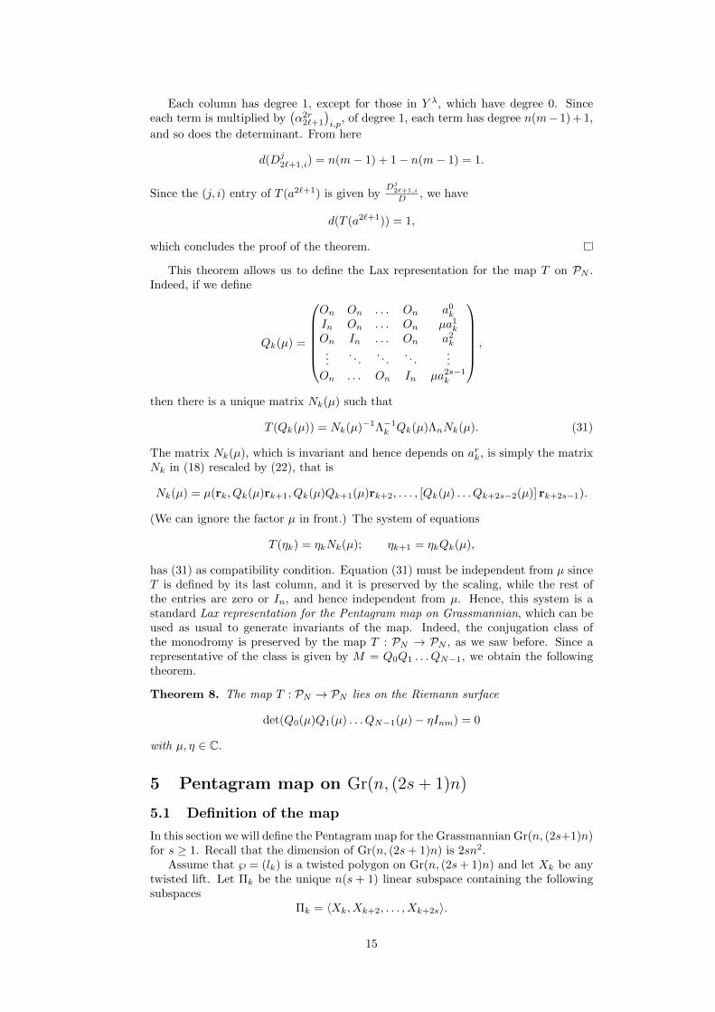
This theorem allows us to define the Lax representation for the map T on PN .Indeed, if we define

Qk(µ) =

On On . . . On a0kIn On . . . On µa1kOn In . . . On a2k...

. . .. . .

. . ....

On . . . On In µa2s−1k

,

then there is a unique matrix Nk(µ) such that

T (Qk(µ)) = Nk(µ)−1Λ−1k Qk(µ)ΛnNk(µ). (31)

The matrix Nk(µ), which is invariant and hence depends on ark, is simply the matrixNk in (18) rescaled by (22), that is

Nk(µ) = µ(rk, Qk(µ)rk+1, Qk(µ)Qk+1(µ)rk+2, . . . , [Qk(µ) . . . Qk+2s−2(µ)] rk+2s−1).

(We can ignore the factor µ in front.) The system of equations

T (ηk) = ηkNk(µ); ηk+1 = ηkQk(µ),

has (31) as compatibility condition. Equation (31) must be independent from µ sinceT is defined by its last column, and it is preserved by the scaling, while the rest ofthe entries are zero or In, and hence independent from µ. Hence, this system is astandard Lax representation for the Pentagram map on Grassmannian, which can beused as usual to generate invariants of the map. Indeed, the conjugation class ofthe monodromy is preserved by the map T : PN → PN , as we saw before. Since arepresentative of the class is given by M = Q0Q1 . . . QN−1, we obtain the followingtheorem.

Theorem 8. The map T : PN → PN lies on the Riemann surface

det(Q0(µ)Q1(µ) . . . QN−1(µ)− ηInm) = 0

with µ, η ∈ C.

5 Pentagram map on Gr(n, (2s + 1)n)

5.1 Definition of the map

In this section we will define the Pentagram map for the Grassmannian Gr(n, (2s+1)n)for s ≥ 1. Recall that the dimension of Gr(n, (2s+ 1)n) is 2sn2.

Assume that ℘ = (lk) is a twisted polygon on Gr(n, (2s+ 1)n) and let Xk be anytwisted lift. Let Πk be the unique n(s + 1) linear subspace containing the followingsubspaces

Πk = 〈Xk, Xk+2, . . . , Xk+2s〉.

15

We define the pentagram map to be the map T taking the polygon ℘ to the uniquetwisted polygon (with the same monodromy) whose kth vertex has a lift given by theintersections Πk ∩Πk+1. This map can be defined either on the space of polygons, oron the vertices. The map T is well defined and independent from the lift X. In fact,from the Grassmann formula we get

(2s+ 1)n = dim(Πk−1 + Πk) = dim Πk−1 + dim Πk − dim(Πk−1 ∩Πk)

= (s+ 1)n+ (s+ 1)n− dim(Πk−1 ∩Πk)

= 2(s+ 1)n− dim(Πk−1 ∩Πk),

which shows that dim(Πk−1 ∩ Πk) = n for any k, and hence Πk ∩ Πk+1 is a lift of aunique element in Gr(n, (2s+ 1)n), an element equals to the kth vertex of T (℘). Asbefore, we will abuse notation and use T equally for the map on polygons, on theirlifts, on frames or on the moduli space.

Clearly the pentagram map is invariant under the action of the projective group(linear on lifts), and therefore one is able to write it as a map on the moduli space ofGrassmannian polygons, as represented by the invariants we found in section 3. Thisis what we do next.

Let us consider a twisted normalized lift V = (Vk) of a regular N -gon, ℘ = (lk)as in theorem 1. Then, using dimension counting, there exist 2s + 1 squared n × nmatrices a0k, a

1k, . . . , a

2s−1k , a2sk such that

Vk+2s+1 = Vka0k + Vk+1a

1k + · · ·+ Vk+2s−1a

2s−1k + Vk+2sa

2sk . (32)

The blocks will be normalized so that a0k is diagonal or Toeplitz, and the entries ofa2sk have a number of syzygies that relate them.

If the lift is twisted, then aik will be N -periodic for i = 0, 1, 2, · · · , 2s; that is

aik+N = aik, (33)

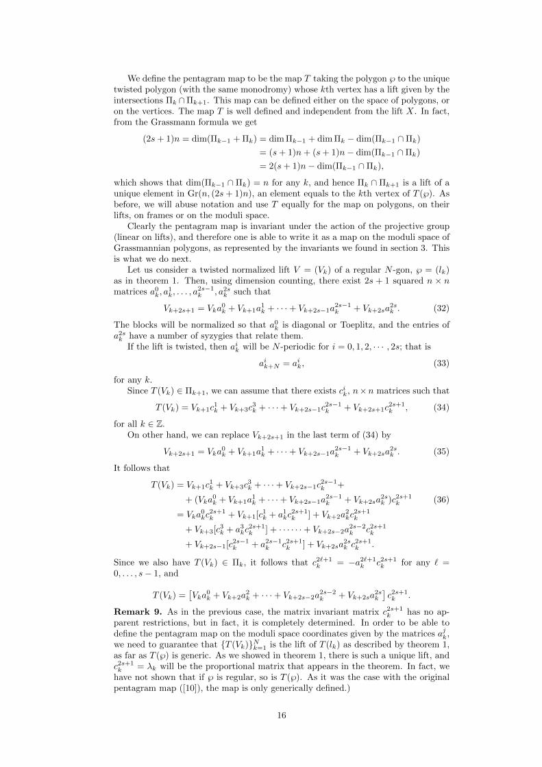
for any k.Since T (Vk) ∈ Πk+1, we can assume that there exists cik, n×n matrices such that

T (Vk) = Vk+1c1k + Vk+3c

3k + · · ·+ Vk+2s−1c

2s−1k + Vk+2s+1c

2s+1k , (34)

for all k ∈ Z.On other hand, we can replace Vk+2s+1 in the last term of (34) by

Vk+2s+1 = Vka0k + Vk+1a

1k + · · ·+ Vk+2s−1a

2s−1k + Vk+2sa

2sk . (35)

It follows that

T (Vk) = Vk+1c1k + Vk+3c

3k + · · ·+ Vk+2s−1c

2s−1k +

+ (Vka0k + Vk+1a

1k + · · ·+ Vk+2s−1a

2s−1k + Vk+2sa

2sk )c2s+1

k (36)

= Vka0kc

2s+1k + Vk+1[c1k + a1kc

2s+1k ] + Vk+2a

2kc

2s+1k

+ Vk+3[c3k + a3kc2s+1k ] + · · · · · ·+ Vk+2s−2a

2s−2k c2s+1

k

+ Vk+2s−1[c2s−1k + a2s−1

k c2s+1k ] + Vk+2sa

2sk c

2s+1k .

Since we also have T (Vk) ∈ Πk, it follows that c2`+1k = −a2`+1

k c2s+1k for any ` =

0, . . . , s− 1, and

T (Vk) =[Vka

0k + Vk+2a

2k + · · ·+ Vk+2s−2a

2s−2k + Vk+2sa

2sk

]c2s+1k .

Remark 9. As in the previous case, the matrix invariant matrix c2s+1k has no ap-

parent restrictions, but in fact, it is completely determined. In order to be able todefine the pentagram map on the moduli space coordinates given by the matrices ajk,we need to guarantee that T (Vk)Nk=1 is the lift of T (lk) as described by theorem 1,as far as T (℘) is generic. As we showed in theorem 1, there is such a unique lift, andc2s+1k = λk will be the proportional matrix that appears in the theorem. In fact, we

have not shown that if ℘ is regular, so is T (℘). As it was the case with the originalpentagram map ([10]), the map is only generically defined.)

16

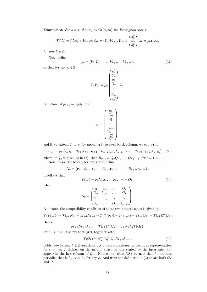
Example 2. For s = 1, that is, on Gr(n, 3n) the Pentagram map is

T (Vk) = (Vka0k + Vk+2a

2k)λk = (Vk, Vk+1, Vk+2)

a0kOna2k

λk = ρkrkλk,

for any k ∈ Z.

Now, defineρk = (Vk Vk+1 . . . Vk+2s−1 Vk+2s), (37)

so that for any k ∈ Z

T (Vk) = ρk

a0kOna2kOn...Ona2sk

λk.

As before, if ρk+1 = ρkQk, and

rk =

a0kOna2k...

a2s−2k

Ona2sk

,

and if we extend T to ρk by applying it to each block-column, we can write

T (ρk) = ρk(rkλk Rk+1rk+1λk+1 Rk+2rk+2λk+2 · · · Rk+2srk+2sλk+2s

), (38)

where, if Qk is given as in (3), then Rk+i = QkQk+1 · · ·Qk+i−1, for i = 1, 2, . . . .Now, as we did before, for any k ∈ Z define

Nk =(rk Rk+1rk+1 Rk+2rk+2 · · · Rk+2srk+2s

).

It follows thatT (ρk) = ρkNkΛk, ρk+1 = ρkQk, (39)

where

Λk =

λk On . . . OnOn λk+1 . . . On. . .

. . .. . .

. . .

On . . . On λk+2s

.

As before, the compatibility condition of these two natural maps is given by

T (T (ρk)) = T (ρkNk) = ρk+1Nk+1 = T (T (ρk)) = T (ρk+1) = T (ρkQk) = T (ρk)T (Qk).

Henceρk+1Nk+1Λk+1 = T (ρk)T (Qk) = ρkNkΛkT (Qk),

for all k ∈ Z. It shows that (39), together with

T (Qk) = N−1k Λ−1

k QkNk+1Λk+1, (40)

holds true for any k ∈ Z and describes a discrete, parameter free, Lax representationfor the map T defined on the moduli space as represented by the invariants thatappear in the last column of Qk. Notice that from (38) we now that λk are alsoperiodic, that is λk+N = λk for any k. And from the definition in (3) so are both Qkand Rk.

17

5.2 A Lax representation for the pentagram map on Gr(n, (2s+1)n

As we did for the even dimensional case, in this section we will prove that one canintroduce a parameter µ in (39) in such a way that (40) will be independent from µ.This will define a true Lax representation that can be used for integration of the map.As it was done in [6], we will prove that the map T is invariant under a scaling, thistime given by

a2r+1k → µ−1+r/sa2r+1

k , r = 0, . . . s− 1 a2rk → µr/sa2rk , r = 0, 1, . . . , s. (41)

We will follow the same steps as in the even dimensional case. The first steps involveproving that the map defined without the proportional matrix λk is invariant underthe scaling. We will then calculate the degree of λk using these results and incorporatethe proportional matrices λk to the map to finally calculate the degree of T (aik).

First of all, notice that if, as before, we denote by Fk+r the r+ 1 block-column ofNk, the analogous to Lemma 4 still holds true. We cite it here without proof, sincethe proof is identical.

Lemma 10. Let Fk = rk and Fk+` = Rk+`rk+`, ` = 1, . . . as above. Then, thereexist n× n matrices αji such that

Fk+2` =∑r=1

Fk+2r−1α2`2r−1 +Gk+2`, Fk+2`+1 =

∑r=0

Fk+2rα2`+12r + Gk+2`+1, (42)

for ` ≥ 1, where

Gk+2`+1 = pk (T Gk+2`)2s + ΓT Gk+2`, α2`+12r = T α2`

2r−1, α2`+10 = (T Gk+2`)2s ,

(43)with

pk =

Ona1kOna3kOn. . .a2s−1k

On

, (44)

andGk+2`+2 = ΓT Gk+2`+1, α2`+2

2r+1 = T α2`+12r , Gk = Fk = rk. (45)

By A2s we mean the last n× n block entry of a matrix A.

The main difference with the even dimensional case is that the even block-columnsG2` start now with a non-zero block (while before it started with a zero one), andgenerate a (s+ 1)n dimensional subspace, orthogonal to those generated by the odd

ones G2`+1, which start with a zero block and generate a sn dimensional subspace.

Also, in this case the first two blocks of G2` are zero since Gk+2` = ΓT Gk+2`−1 andΓ shifts all the blocks once downwards.

Assume first that we drop the Λk factor and define

T (Vk) = ρkrk.

Define also cik = T (aik), which is given by the compatibility formula below, the anal-ogous to (29)

T (Qk) = N−1k QkNk+1.

ThenT (ak) = N−1

k QkT Fk+2s = N−1k Fk+2s+1,

18

which can be written asNkT (ak) = Fk+2s+1. (46)

Once more T (ak) can be interpreted as the solution of the linear equation (46).

Theorem 11. The matrices cik are homogenous with respect to the scaling (41), and

d(c2`k ) =`

s, d(c2`+1

k ) = −1 +`

s.

Notice that the degree of crk coincides with that of ark. Later we will show that λkare all invariant under scaling and this theorem will essentially prove the invarianceof the map under (41).

Let us once more drop the subindex k unless needed. As we did in the previouscase, we will work with determinants of the form Dj

r,i, simplifing them down to theirhomogeneous component, and calculating their degree. Because they are solution of(46), each entry of cr will be a quotient of these determinants and D, and this waywe will be able to determine their degree. The study comes in a number of lemmas.

Lemma 12. The determinant

D = det(F, F1, . . . , F2s),

is invariant under (41).

Proof. Using (42) we have that

D = det(F, G1, G2, . . . , G2s−1, G2s).

This time all G2r = ΓT G2r−1 have the first two blocks equal On; therefore, the blocksin the first row of D are all zero, except for the first block which is the first block ofF = r, i.e. a0, and which is invariant under scaling. If we simplify using the first nrows, we have the determinant of a matrix that looks like

A1,1 On A1,2 On . . . A1,s OnOn B1,1 On B1,2 . . . On B1,s

A2,1 On A2,2 On . . . A2,s OnOn B2,1 On B2,2 . . . On B2,s

... . . . . . . . . . . . . . . . . . .As,1 On As,2 On . . . As,s OnOn Bs,1 On Bs,2 . . . On Bs,s

,

where Ai,j are the nonzero blocks of G2j−1 and Bi,j are the nonzero blocks of G2j .Using n2s(s − 1) exchanges of rows and columns, this determinant can be easilytransformed into

det

(A OsnOsn B

),

with A = (Ai,j) and B = (Bi,j). Also, since G2` = ΓT G2`−1, we have that B = T Aand D = detAdet T A.

We will next show that d(Ai,j) = i−js . This will imply, from the definition of

determinant, that d(detA) = n∑si=1

∑sj=1

i−js = 0, concluding the proof.

Indeed, from (43) we have

G2`+1 = p (T G2`)2s + ΓT G2` = p(T 2G2`−1

)2s−1

+ Γ2T 2G2`−1,

and using this we conclude that

Ak,`+1 = a2k−1T As,` + T 2Ak−1,`. (47)

19

The degrees of the nonzero blocks of p are given by

−1, −1 +1

s, −1 +

2

s, . . . , −1 +

s− 1

s,

while the degree of a2s is 1. Thus,

d(Ak,1) = d(a2k−1a2s) = d(T a2k−2) =k − 1

s.

We now use induction. Assume that d(Ai,j) = i−js for all i = 1, . . . s and all j < `.

From (47) we have that, since d(a2k−1) = −1 + k−1s ,

d(a2k−1T 2As,`) = −1 +k − 1

s+s− `s

=k − `− 1

s; d(T 2Ak−1,`) =

k − 1− `s

,

and so

d(Ak,`+1) =k − (`+ 1)

s,

concluding the proof of the lemma.

Let us denote by Djr,i the determinant given by

Djr,i = det(F, F1, . . . , Fr−1, F

jr,i, Fr+1, . . . , F2s),

where F jr,i is the block-column obtained from Fr by substituting the ith column, f ir,

with the jth column of F2s+1, f j2s+1.

Lemma 13. Determinant Dj2`+1,i is homogeneous for all i, j = 1, . . . n, and ` =

0, . . . , s− 1, and

d(Dj2`+1,i) = −1 +

`

s.

Proof. As in the previous cases we will make heavy use of (42) to reduce the determi-nants to their homogeneous components before calculating their degree. First of allwe will substitute the ith column of F j2`+1,i in

det(F, F1, . . . , F2`, Fj2`+1,i, F2`+2, . . . , F2s),

by that of G2s+1, gj2s+1, since the difference is a combination of even columns, whichare all present in the determinant. We can then simplify the columns to the right ofthis and substitute them by either G2r+1 or by

G2r + gi2`+1

(α2r2`+1

)i,

where a super index indicate the column, a subindex the row. We can then substituteall the remaining columns of F j2`+1,i and Fr, r ≤ 2` by those of Gr or Gr, dependingon parity, to obtain

Djr,i = det(F, G1, . . . , G2`, G

j2`+1,i, G2`+2+gi2`+1

(α2`+22`+1

)i, G2`+3, . . . , G2s+g

i2`+1

(α2s2`+1

)i),

where Gj2`+1,i is equal to G2`+1 except for its ith column which has been substituted

by the jth column of G2s+1. Since the missing column in G2`+1 has been substitutedby another odd column, if we expand this determinant all the terms that include anyextra column gi2`+1 will vanish since we already have odd columns equal to half thedimension in their standard position. Therefore

Djr,i = det(F, G1, . . . , G2`, G

j2`+1,i, G2`+2, G2`+3, . . . , G2s).

Consider now the following product

gj2s+1 = gi2`+1 ⊗ (gi2`+1)−1 ⊗ gj2s+1, (48)

20

where by (gi2`+1)−1 we mean the vector whose entries are the inverses of the entries ofgi2`+1, and where the product represents the individual entries product, as customary.

We claim that (gi2`+1)−1 ⊗ gj2s+1 is homogeneous, each entry with the same degree.

Indeed, using the fact that d(Ai,j) = i−js (recall that Ai,j , i = 1, . . . s, are the nonzero

blocks of G2j−1, j = 1, . . . , s), we can see that

d((gi2`+1)−1 ⊗ gj2s+1) = d(gj2s+1)− d((gi2`+1)

= (∗,−1, ∗,−1 +1

s, ∗, . . . , ∗,−1 +

s− 1

s, ∗)

− (∗,− `s, ∗, 1− `

s, ∗, . . . , ∗, s− 1− `

s, ∗)

= (∗,−1 +`

s, ∗,−1 +

`

s, ∗, . . . , ∗,−1 +

`

s, ∗),

where ∗ indicates the position of a zero block. Therefore, substituting gj2s+1 by (48)in the determinant, expanding the determinant using this column, and using the factthat D is invariant under scaling gives us

d(Dj2`+1,i) = −1 +

`

s,

as claimed.

Lemma 14. Determinant Dj2`,i is also homogeneous for all i, j = 1, . . . , n, ` =

0, . . . , s− 1 and

d(Dj2`,i) =

`

s.

Proof. The proof of this case is a bit more complicated. We need to look at thedeterminant

Dj2`,i = det(F, F1, . . . , F2`−1, F

j2`,i, F2`+1, . . . , F2s).

As before, we simplify the ith column of F j2`,i, using (42). That is, f j2s+1 will besubstituted by

gj2s+1 + f i2`(α2s+12`

)i,j. (49)

We can then substitute the columns to the right of this one: we substitute F2r+1 by

G2r+1 + f i2`(α2r+12`

)i

and F2r by G2r. We can also substitute f i2` in the expression of

F2r+1 by gi2`. We then change the remaining columns in F j2`,i, including f i2`, by those

of G2` (we call the resulting matrix Gj2`,i), and substitute the F ’s blocks to the left

of Gj2`,i by G-blocks. Then, column (49) becomes

gj2s+1 + gi2`(α2s+12`

)i,j. (50)

and the resulting determinant is given by

det(F, G1, G2 . . . , G2`−1, Gj2`,i, G2`+1+gi2`

(α2`+12`

)i, G2`+2, . . . , G2s−1+gi2`

(α2s+12`

)iG2s).

If we now expand the determinant using the ith column of Gj2`,i, i.e. (50), we have

Dj2`,i =

(α2s+12`

)i,jD

+ det(F, G1, G2 . . . , G2`−1, Gj2`,i, G2`+1 + gi2`

(α2`+12`

)i, G2`+2, . . . , G2s−1 + gi2`

(α2s+12`

)iG2s),

where Gj2`,i has as ith column gj2s+1 and G2` elsewhere.

Notice that, once more, if we expand this determinant, the terms with no Gi2` willbe zero since we have more odd columns that are needed to generate the odd subspace

21

(indicated with a hat) given that Gj2`,i contains one. Thus, the determinant expandsas

s−1∑r=`+1

n∑p=1

(α2r+12`

)i,p

det(F, G1, G2, . . . , Gj2`,i, G2`+1, . . . , G

p2r+1+gi2`e

Tp , G2`+1, . . . , G2s),

where Gp2r+1 indicates G2r+1 with a zero p column. Each one of these terms can

transformed by shifting the p column of Gp2r+1 + gi2`eTp and the ith column of Gj2`,i.

The expansion becomes

s−1∑r=`+1

n∑p=1

±(α2r+12`

)i,p

det(F, G1, G2, . . . , G2`, G2`+1, . . . , Gp2r+1+gj2s+1e

Tp , G2`+1, . . . , G2s),

(51)and now we are ready to calculate degrees. Substitute gj2s+1 by

gj2s+1 = gj2s+1 ⊗ (gp2r+1)−1 ⊗ gp2r+1,

as before, and notice that the degree of gj2s+1 ⊗ (gp2r+1)−1 is the same for all of itsblock-entries and equal to −1 + r

s

d(gj2s+1 ⊗ (gp2r+1)−1) = d(gj2s+1)− d(gp2r+1) =

∗1−(s+1)

s∗

2−(s+1)s...

s−(s+1)s∗

−

∗1−(r+1)

s∗

2−(r+1)s...

s−(r+1)s∗

.

We now need to calculate the degree of αji . This is simple from (43) and (45). Wesee that

d(α2r+10 ) =

s− rs

, d(α2r+12` ) = d(α

2(r−`)+10 ) = 1− r − `

s,

d(α2r2`+1) = d(α

2(r−`−1)+10 ) = 1− r − `− 1

s.

With this, every term in the expansion (51) has degree

−1 +r

s+ d(

(α2r+12`

)i,p

) = −1 +r

s+ 1− r − `

s=`

s,

and since

d((α2s+12`

)i,jD)

= d((α2s+12`

)i,j

)= 1− s− `

s=`

s,

we conclude the proof of the lemma.

After these results, the proof of theorem 11 is immediate since the entry (j, i) ofcr is the quotient

Djr,i

D,

and so d(cr) = d(Djr,i), which coincide with the statement of the theorem.

Finally, the following theorem is a consequence of 11.

Theorem 15. If N and m are coprime, the map T is invariant under the scaling(41).

22

Proof. To prove this result we simply need to prove that λk are invariant under scaling.After this fact is proved, computations similar to those in the proof of theorem 7 willshow that even as we introduce λk in the different block columns of determinants Dand Dj

`,i, they do alter neither the homogeneity nor the degree of the determinantsbecause they are invariant under the scaling and all columns of a block-column havethe same degree (and so do their linear combinations). Therefore

d(crk) = d(T (ark)) = d(ark),

for any k and r = 0, . . . ,m − 1. We will avoid further details of those computationssince they are almost identical to those in 7 and the interested reader can reproducethem.

To show that λk are invariant under scaling is not hard: if N and m are coprime,their determinants, δk = detλk, are the unique solution of

detNkδkδk+1 . . . δk+m−1 = 1,

and since detNk = Dk, detNk is invariant under the scaling (since d(Dk) = 0) and soare δk for any k. We next look at each factor in the splitting of λk = dkqk. As in theprevious case, the factors dk are determined by the normalization of Bk = Πm(c0k) asin (7), and since c0k are invariant under the scaling, so will dk.

Finally, qk are uniquely determined by equations of the form (11) and (12) forcm−1k , and by their determinants. Since cki,j = cm−1

k−m+1cm−1k−m+1 . . . c

m−1N+k−m is homo-

geneous, equations (11)-(12) are scaling invariant. Furthermore, det qk = det d−1k δk

and both δk and det dk are scaling invariant, so is det qk. Therefore, qk are scalinginvariant and so are λk.

As in the even dimensional case, this theorem allows us to define the Lax repre-sentation for the map T : PN → PN . Indeed, if we define

Qk(µ) =

On On On . . . On On a0kIn On On . . . On On µ−1a1kOn In On . . . On On µ

1s a2k

On On In . . . On On µ−1+ 1s a3k

.... . .

. . .. . .

......

...

On On . . . On In On µ−1+ s−1s a2s−1

k

On On . . . On On In µa2sk

,

then we can define

Nk(µ) = (rk(µ), Rk(µ)rk+1, Rk+1(µ)rk+2(µ), . . . , Rk+m−2(µ)rk+m−1(µ)),

where

rk(µ) =

a0rOnµ

1s a2rOnµ

2s a4r...Onµask

,

and Rk+r(µ) = Qk(µ)Qk+1(µ) . . . Qk+r(µ). The compatibility condition of the system

ρk+1 = ρkQk(µ), T (ρk) = ρkNk(µ),

will be given byT (Qk(µ)) = Nk(µ)−1Λ−1

k Qk(µ)ΛnNk(µ). (52)

23

Equation (52) must be independent from µ since T is defined by its last column,and it is preserved by the scaling, while the rest of the entries are zero or In, andhence independent from µ. Hence, this system is a standard Lax representation forthe Pentagram map on Grassmannian in the case m = 2s+ 1, which can also be usedas usual to generate invariants of the map. With this new scaling, theorem 8 is alsotrue in the case when m is odd.

Acknowledgements: This paper is supported by Marı Beffa’s NSF grant DMS#1405722, by Felipe’s CONACYT grant #222870, and by the hospitality of the Uni-versity of Wisconsin-Madison during Felipe’s sabbatical year. R. Felipe was alsosupported by the Sistema de ayudas para anos sabaticos en el extranjero, CONACYTprimera convocatoria 2014.

References

[1] B. Khesin and F. Soloviev, Integrability of higher pentagram maps, Math. An-nalen, vol. 357 (2013), 1005-1047.

[2] B. Khesin and F. Soloviev, The geometry of dented pentagram maps, J. of Europ.Math. Soc., (2013).

[3] I. Krichever, Commuting difference operators and the combinatorial Gale trans-form. arXiv: 1403.4629v1[math.AG] 18 Mar 2014.

[4] E. Mansfield, G. Marı Beffa and J. P. WangDiscrete moving frames and integrablesystems, Foundations of Computational Mathematics, Volume 13, Issue 4 (2013),pp 545-582.

[5] G. Marı Beffa, On generalizations of the pentagram map: discretizations of AGDflows, Journal of Nonlinear Science: Volume 23, Issue 2 (2013), Page 303-334.

[6] G. Marı Beffa, On Integrable Generalizations of the Pentagram Map, InternationalMathematics Research Notices, (2015) (12): 3669-3693;doi: 10.1093/imrn/rnu044.

[7] G. Marı Beffa, On the integrability of the shift map on twisted pentagram spirals,J. Phys. A: Math. Theor. 48 (2015) 285202

[8] V. Ovsienko, R. E. Schwartz and S Tabachnikov, The Pentagram map: A discreteintegrable system, Communications in Mathematical Physics 299 (2010) pp 409-446

[9] V. Ovsienko, R. E. Schwartz and S Tabachnikov, Liouville-Arnold integrabilityof the pentagram map on closed polygons Duke Mathematics Journal, Vol 162,Number 12 (2012) pp 2149-2196

[10] R. E. Schwartz, The Pentagram Map, Journal of Experimental Mathematics(1992) V. 1 pp. 85-90

[11] R. E. Schwartz, The Projective Heat Map Acting on Pentagons, Research mono-graph (2014).

[12] R. E. Schwartz, Pentagram Spirals, J. Exp Math. Vol 22, Issue 4 (2013)

[13] F. Soloviev, Integrability of the Pentagram Map, Duke Math. Journal, vol. 162(2013), no.15, 2815–2853.

24