The Performance of

Emerging Hedge Fund Managers

Rajesh K. Aggarwal

and

Philippe Jorion*

This version: January 8, 2008

Draft

* Aggarwal is with the Carlson School of Management, University of Minnesota. Jorion is with the Paul Merage School of Business, University of California at Irvine and Pacific Alternative Asset Management. The paper has benefited from the comments and suggestions of Jim Berens, Jane Buchan, Judy Posnikoff, Patricia Watters, and seminar participants at UC-Irvine.

Correspondence can be addressed to:

Philippe Jorion Rajesh K. Aggarwal Paul Merage School of Business Carlson School of Management University of California at Irvine University of Minnesota Irvine, CA 92697-3125 Minneapolis, MN 55455 (949) 824-5245, E-mail: pjorion@uci.edu (612) 625-5679, Email: aggar015@umn.edu

© 2007 Aggarwal and Jorion

2

The Performance of

Emerging Hedge Fund Managers

ABSTRACT

This paper provides the first systematic analysis of performance patterns for emerging

managers in the hedge fund industry. Emerging managers have particularly strong financial

incentives to create investment performance and, because of their size, may be more nimble than

established ones. Performance measurement, however, needs to control for the usual biases

afflicting hedge fund databases. Backfill bias, in particular, is severe for this type of study. After

adjusting for such biases and using a novel event time approach, we find strong evidence of

outperformance during the first two to three years of existence. Controlling for size, each additional

year of age decreases performance by 48 basis points, on average. Cross-sectionally, early

performance by individual managers is quite persistent, with early strong performance lasting for up

to five years.

JEL Classifications: G11 (portfolio choice), G23 (private financial institutions), G32 (financial risk management)

Keywords: hedge funds, emerging managers, incentives, performance evaluation

3

I. Introduction

The hedge fund industry has grown very rapidly. Assets under management have increased

from an estimated $39 billion in 1990 to more than $1,400 billion in 2006.1 Correspondingly, the

number of managers has increased from 530 to more than 7,200. One immediate question with the

large growth in the number of managers is whether all of these new managers are capable of

generating superior performance. This paper provides the first systematic evidence on whether

emerging hedge fund managers tend to outperform more established ones. We find that emerging

managers tend to add value in their early years. This effect is slightly stronger for larger funds.

Thereafter, performance tends to deteriorate. This is consistent with the implications of stronger

incentive effects for emerging managers, but mainly for those that start up with a larger pool of

capital. Controlling for size, each additional year of fund age decreases fund performance by 48 basis

points, on average, which suggests that emerging funds, especially in the first two years of life,

represent attractive investment opportunities.

The growth of the hedge fund industry can be rationalized by the value added generated by

hedge fund managers that we document. For example, over the period 1994 to 2006, the CSFB hedge

fund index delivered an additional 6.8% annual return over cash.2 Put differently, this is the same

performance as the S&P stock market index, but with half the volatility and very little systematic risk.

These performance results are puzzling in view of the mutual fund literature, which finds that mutual

funds generally fail to outperform their benchmarks even after adjusting for risk. Hedge funds,

however, differ in a number of essential ways from mutual funds. They provide more flexible

1 According to the HFR (2007) survey, excluding funds of funds to avoid double-counting. 2 The CSFB hedge fund index, which in absolute terms returned 10.9% per annum over this period, is representative of all hedge funds and does not represent the returns on emerging hedge funds alone. For emerging hedge funds, see Table 1.

4

investment opportunities and are less regulated.3 Hedge fund managers also have a stronger financial

motivation to perform because of the compensation structure typical of hedge funds: this includes not

only a fixed annual management fee that is proportional to assets under management but also an

incentive fee that is a fraction of the dollar profits. In addition, hedge fund managers often invest a

large portion of their own wealth in the funds they manage.

At the same time, there is a fair amount of interest in “emerging” managers, defined as

newly-established managers. In this paper, we define emerging hedge fund managers as recently-

established funds, using fund age or years of existence since inception, as the primary sorting

criterion.4 We focus on emerging managers for several reasons. Incentive effects should be

stronger for this class of hedge fund managers. The marginal utility of a given annual profit should

be higher for managers with lower initial wealth; given that emerging managers should be on

average younger than more established managers, profits can be expected to accrue over a longer

lifetime. In addition, because of their size, they may be more nimble than established managers.

Finally, emerging managers are much more likely to be open to investors than are established hedge

funds, especially established funds with strong historical performance.

So far, no academic paper has directly investigated the effect of fund age on hedge fund

performance. Age sometimes appears as another factor explaining performance in mutual funds,

with generally insignificant effects. Crucially, the age factor in hedge funds is subject to a very

significant backfill bias or instant-history bias. This bias occurs because managers report their

performance to the databases only voluntarily—there is no requirement that managers disclose

performance. Typically, after inception, the fund’s performance is not made public during some

3 More flexible investment opportunities include the ability to short securities, to leverage the portfolio, to invest in derivatives, and generally to invest across a broader pool of assets. The lighter regulatory environment creates an ability to set performance fees, lockup periods, or other forms of managerial discretion.

5

incubation period. Upon good performance, the manager is more likely to make the performance

public. If so, the manager starts reporting to the database current performance and backfills the past

performance, and not even necessarily over the entire incubation period. Funds that collapse due to

poor performance may never appear in the database.

Our paper eliminates backfill bias by selecting a sample of funds with inception dates very

close to the start dates in the database. We find that that the backfill bias would otherwise

completely distort measures of early performance, imparting an upward bias of around 5% in the

first three years. We also find that the common practice of arbitrarily dropping the first 12 or 24

months of the sample is insufficient to control for backfill bias. In addition, it may bias tests of

persistence toward non-rejection because performance during the backfill period generally appears

very high.

Our paper provides evidence on whether emerging hedge fund managers tend to outperform

more established ones. After eliminating backfill bias, we examine fund performance in “event

time” where the event is the start of fund performance. Examining funds in event time is a more

powerful and direct method to assess the relationship between age and performance. To see this,

suppose that every year a large number of new funds start up, and that new or emerging funds

outperform existing funds. Running pooled cross-sectional regressions of fund returns on indices or

factors (even with time fixed effects) in calendar time would imply that hedge funds outperform on

average. However, the outperformance is actually generated by the new funds, an effect which will

be captured in event time but missed in calendar time.

Our use of event time is novel in hedge fund research, and the event time approach is ideally

suited for examining the performance of emerging hedge funds. Conventional event studies

4 Recently established funds are taken as a proxy for emerging managers. It is possible, however, that a recently established fund is run by a manager who has run other hedge funds. With this caveat, we use the terms emerging

6

typically examine short horizon reactions to news or events. More recently (and perhaps

controversially), long horizon event studies have been used to examine differences in firm returns

due to changes that cannot precisely be pinned down to the day. Our use of event time is long

horizon in nature—we examine hedge fund performance over years—but we know precisely when

the hedge fund starts reporting performance. We use event time to measure hedge fund aging,

which is similar to a cohort analysis, while still allowing us to create portfolios of hedge funds.

Using portfolios allows us to test hypotheses while automatically accounting for correlations

in returns across funds. This is because the standard errors we report are based on portfolio returns.

In contrast, pooled cross-sectional regressions of individual fund returns are usually misspecified

due to cross-sectional correlations in fund returns. Our econometric approach yields robust

evidence that emerging managers tend to add value in their early years. In addition, when we form

portfolios of emerging funds, we find that early performance (up to five years) is persistent.

Importantly, the persistence we find is present both for the best performing quintile and the worst

performing quintile of hedge funds. This result is important, as earlier studies of performance

persistence tend to find performance persistence amongst only the worst performing furnds. As

hedge funds become more established (i.e., age) the performance persistence that we document

fades away, along with the outperformance exhibited in the funds’ early years.

In further tests, we perform a cohort analysis, where we track over time all funds that start

within a given year. This analysis allows us to more precisely control for changes in fund size. One

possibility is that past good performance may lead to inflows, which results in the deterioration of

fund performance over time, as in Berk and Green (2004). Under these conditions, the deterioration

in fund performance is actually due to changes in fund size, and not fund age. When we control for

managers, new managers, and new funds interchangeably.

7

fund size, we continue to find that younger funds perform better and this performance deteriorates

over time.

This paper is structured as follows. We review the rationale for emerging managers and

relevant literature in Section II. Section III then describes the data and empirical setup. Section IV

discusses the results. Concluding comments are contained in Section V.

II. The Rationale for Emerging Managers

Emerging managers may be attractive for a number of reasons. The first set of arguments is

related to incentive effects. There are good reasons to believe that incentive effects are particularly

important for the hedge fund industry. Incentives should help sort managers by intrinsic skills. We

would expect the best asset managers to migrate to the hedge fund industry. In addition, incentives

should induce greater effort by managers, as predicted by agency theory.5 In the mutual fund

industry, Massa and Patgiri (2007) compare the usual fixed management fee setup with arrangements

where this fee decreases as a function of asset size. This concave function provides a negative

incentive effect, which is found to be associated with worse performance, as predicted. In the hedge

fund industry, Agarwal et al. (2007) find that greater managerial incentives, managerial ownership,

and managerial discretion are associated with superior performance. In addition, these effects explain

the empirical evidence of return persistence for hedge funds, while little persistence has been reported

for mutual funds.6

5 See for instance Jensen and Meckling (1976). 6 Jagannathan et al (2007) find evidence of persistence in hedge fund returns over 3-year horizons. They also provide a review of the literature on persistence in hedge fund returns. Kosowski, Naik, and Teo (2007) report mild evidence of persistence using classical OLS alphas but much stronger evidence in a Bayesian analysis. Baquero et al. (2005) report persistence at the quarterly and annual horizons, using raw and style-adjusted returns. Aggarwal, Georgiev, and Pinato (2007) show performance persistence for time horizons ranging from six months to over two years. Carhart (1997) reports no evidence of persistence in mutual fund returns using abnormal returns defined by a 4-factor model. These conclusions are reinforced by Carhart et al. (2002), who deal with survivorship and look-ahead biases for mutual funds.

8

Relative to more established and older managers, incentive effects should be even more

important for emerging managers because their initial wealth is smaller. The marginal utility of the

same dollar amount of fees should progressively decrease as the manager gets richer. In addition, the

benefits of high-powered incentive contracts carry over a longer period, since emerging managers are

generally younger. So, emerging managers should put more effort into enhancing performance. In

their starting years, managers may also be more focused on generating performance rather than

spending time marketing to new investors.

The second set of arguments for emerging managers is related to size. They generally

manage a smaller asset pool than the typical fund. Goetzmann et al. (2003) argue that arbitrage

returns may be limited, leading to diseconomies of scale. They report that, in contrast with the

mutual fund industry, large hedge funds frequently prefer not to grow. Diseconomies of scale also

underpin Berk and Green (2004)’s model that explains many regularities in the portfolio

management industry that are widely regarded as anomalous. Managers with skill attract inflows,

but diseconomies of scale erode performance. As a result, the performance of skilled managers

disappears over time. Getmansky (2004) studies competition in the hedge fund industry and finds

decreasing returns to scale.

For mutual funds, however, the evidence is mixed. Grinblatt and Titman (1989) and

Wermers (2000) find no significant difference across the net performance of small and large funds.

Chen et al. (2004) report some evidence of a negative relationship between fund returns and size,

but this is exclusively confined to funds that invest in small stocks, which tend to be illiquid. This

is confirmed by Allen (2007), who reports no difference across size for institutional investors except

for the small cap category, which is capacity-constrained and for which small funds perform better.

Another set of arguments for emerging managers is that they may have newer ideas for trades,

whose usefulness can fade away over time. New funds may be established to take advantage of new

9

markets or new financial instruments. Finally, irrespective of a performance advantage, emerging

managers are usually open to new investors and as a result, represent practical investment

opportunities in hedge funds.

So far, no academic paper has directly investigated the effect of fund age on hedge fund

performance.7 Age sometimes appears as another factor explaining performance in mutual funds,

with generally insignificant effects. In addition, the age factor is subject to a very significant

backfill bias or instant-history bias with hedge funds. This bias arises from the option to report

performance or not, and if so, to backfill performance produced during an incubation period.

Interestingly, Evans (2007) reports a substantial incubation bias for mutual funds which

parallels the backfill bias in hedge funds. Apparently, mutual fund families seed new funds

without initially making their performance public. After a while, the fund may acquire a ticker

symbol from the NASD, thus becoming public. Evans (2007) defines a fund as incubated if the

period between the ticker creation date and the fund inception date is greater than 12 months. He

reports a difference in performance of 4.7% between incubated funds during their incubation period

and an age-matched sample of non-incubated funds.

Fung and Hsieh (2000) describe the distribution of this incubation period for hedge funds.

The median period is about 12 months based on the TASS database from 1994 to 1998. Fung and

Hsieh (2000) then adjust for this bias by dropping the first 12 months of all return series. The

adjusted series has an average return of 8.9%, against a 10.3% return for the raw series, yielding a

7 Some industry studies purport to demonstrate that young funds perform better. For example, Howell (2001) claims that young funds outperform old funds by 970 basis points on average. This analysis, however, fails to control for backfill bias. Similarly, Jones (2007) claims that young funds (with age less than 2 years) outperform old funds (with age greater than 4 years) by 566 basis points.

10

bias estimate of 1.4% per annum.8 The common practice in hedge fund academic research has

become to drop the first 12 or 24 months to control for backfill bias.9

This adjustment, however, is peculiar. For funds with no instant history, this discards the

first year of performance, which is perfectly valid and very informative. Moreover, for the 50% of

funds with instant-history longer than 12 months, this still preserves a backfill bias. Whether this

biases the results of the empirical analysis depends on the research objective. Clearly, backfill bias

is of first-order importance when evaluating the initial performance of emerging managers. A better

method to control for backfill bias is to minimize the period between inception of the fund and the

first date of entry into the database.10 Thus, we focus on the group of funds for which there is no (or

very little) backfill bias.

In addition, traditional performance evaluation of hedge funds can be subject to survivorship

bias, which arises when dead funds are excluded from the analysis. Fung and Hsieh (2000) estimate

this bias at around 3%. To evaluate the effect of age, it is crucial to control for backfill bias, which

would otherwise make early returns look better. Survivorship bias works in the other direction,

making longer returns look better. Our analysis controls for both backfill and survivorship biases.

The age effect that is the focus of our study is also related to the literature on career

concerns of portfolio managers. For mutual funds, Chevalier and Ellison (1999) indicate that

termination is more sensitive to performance for younger managers. Combined with the incentive

structure in this industry, they argue that this should lead to less risk taking in younger managers.

This is confirmed by their data. Given the vastly different incentives schemes, it is not clear

whether these results should carry over to the hedge fund industry, however. Boyson (2005)

8 Malkiel and Saha (2005) also report estimates of this backfill bias over 1994 to 2003. 9 Kosowski, Naik, and Teo (2007) combine the TASS, HFR, CISDM, and MSCI database, adjusting for backfill bias by dropping the first 12 months of every fund. 10 Such information is available from the TASS and HFR databases.

11

apparently finds opposite effects, which are difficult to interpret due to her grouping by age deciles,

thereby creating nonlinear effects in age measures.

III. Data and Setup

A. Database

The database employed has been collected by Tremont Advisory Shareholders Services

(TASS), which compiles fund data over the period November 1977 to December 2006. The TASS

database covers close to one-half of the estimated total number of hedge funds in existence. The

database provides total monthly returns net of management and incentive fees, as well as assets

under management (AUM). For our analysis, we use data starting in January 1996, the first year

for which there is a non-trivial number of non-backfilled funds, using the method defined below.

TASS reports two separate databases, one with “live” funds and another with “graveyard”

funds, which keeps track of dead funds and starts in 1994. Many funds stop reporting at some

point, because of liquidation or some other reason. We include the graveyard database to minimize

survivorship biases. We eliminate funds of funds as well as duplicate classes from the same fund

family. In addition, we only retain funds that provide returns in U.S. dollars and net of fees.

While eliminating duplicate classes and funds providing returns in currencies other than US

dollars is sufficient to eliminate most situations of the same fund appearing multiple times in the

data, it does not completely resolve the problem. For example, two funds can appear in the

database, be run by the same manager, and have the same name up to one fund having the

designation “onshore” and the other having the designation “offshore.” As another example, two

funds can have the same manager and the same name up to one fund being an “LP” (limited

partnership) and the other being “limited” or an “investment company.” These situations often

happen in fund companies set up with a master-feeder fund structure, where multiple feeder funds

12

channel capital to one investing master fund. In these situations, if the funds are duplicates (for

example, if the returns are identical), we eliminate one of the duplicates.

TASS also provides an “inception date,” a “performance start date,” as well as a “date added

to database.” The inception date is the inception date of the legal fund structure and generally will

not coincide with the start of actual fund investment and performance. The performance start date

is the date of the first reported monthly return. The date added to TASS is when the fund chooses to

start reporting to TASS. For a typical fund in the TASS database, the inception date is prior to the

performance start date, and the performance start date is prior to the date added to the database.

Backfill occurs when the performance start date is before the date the fund was added to the

database. The difference is the “backfill period.” We find that the median backfill period in the

entire database is 480 days, which is substantial. In addition, 37% of funds have a backfill period

longer than two years; 25% of funds have a backfill period longer than 1165 days, which is more

than three years. The obvious concern here is that funds only choose to report to TASS if past

performance has been good and this performance is then allowed to be backfilled.

To control for this effect, we separate the sample into a non-backfilled sample and a

backfilled sample. We define a fund as “non-backfilled” if the period between the inception date

and date added to the database is below 180 days. Note that this definition slightly differs from the

traditional definition of the backfill period, which is the difference between the performance start

date and the date added to the database. Our definition takes into account the possibility that funds

may have actual performance that they choose not to report between the inception date and the

performance start date (which is self-chosen and reported). Our focus on the difference between the

inception date and the date added to the database minimizes both backfill bias and the possibility of

omitted performance. At the same time, the lag of 180 days is required because very few funds

report to the TASS database immediately at inception. For many funds, not reporting performance

13

at inception is entirely legitimate as the fund may be gathering assets rather than investing. The

remaining period between the performance start date and date added to TASS is minimal, with a

median of 82 days. Our use of a window of 180 days for non-backfilled funds is in fact much more

stringent than the 12-month window used by Evans (2007) in the context of mutual fund incubation

bias. As we will show later, our results are not driven by this window.

B. Time Alignment

We perform two types of analysis, based on “event time” and “cohort by calendar year.” In

the first method, the event is the start of fund performance. We form an equally-weighted portfolio

of funds aligned on the first month of reported performance. Using an equal-weighted average

represents the expected return from a strategy of randomly picking managers sorted by these

characteristics. To transform to yearly returns, we cumulate the first 12 months of performance,

which is called year 1. The second twelve month period is then called year 2, and so on. From

January 1996 to December 2006, we have at most 132 months in event time, which could only be

achieved for a fund starting in January 1996 that survives until December 2006 (there are three such

funds).

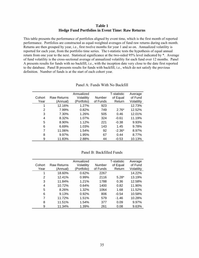
Panel A in Table 1 reports raw returns for our portfolio of emerging funds. We have 923

funds that start (beginning of event year 1) over the period 1996 to 2006 that are free of backfill

bias. By the beginning of event year 2, this number falls to 749, due to fund attrition as well as

truncation at the end of the sample (i.e., a fund that starts in 2006 will not have two years of

performance). By the beginning of event year 9, there are only 44 funds in the portfolio. The last

two years are not reported in the table due to the small number of data points. This process leads to

the largest number of funds in the first month, as every fund in the database with no backfill has at

least one month of performance, and a smoothly decreasing number of funds in event time. Note

14

that the first year performance for these funds is substantially higher than for subsequent years. The

average raw return is 12.16% in the first year. This falls to 7.99% in the second year, which

suggests outperformance by emerging managers. During the first two years, average performance is

10.1%, versus 9.1% during the remaining seven years.

Panel A also displays the portfolio volatility, annualized from monthly data. Volatility is

very low given the large number of funds in the portfolio and the aggregation process across time.

As event time goes by, the volatility increases due to the smaller number of funds in the portfolio.

This volatility is also the standard error of the annual return.11 Thus the estimated annual return

becomes less reliable as time goes by. The table also shows the t-statistic that tests equality of

consecutive annual returns. The return drop from the first to the second year is significant. Note

that what matters is not the level nor sign of returns but rather their patterns over time. Performance

is measured relative to the universe of funds, assuming all returns are drawn from the same

distribution. Later, we will make adjustments for risk and contemporaneous correlations across

funds.

As noted before, it is essential to correct for backfill bias in the TASS data given our interest

in emerging managers. To illustrate this point, Panel B in Table 1 repeats the analysis using all

emerging managers in the TASS data from 1996 to 2006 that do not meet our definition for no

backfill. In other words, these are the backfilled funds. The returns are event time returns, which

are therefore comparable to the returns in Panel A. There are many more backfilled funds than non-

backfilled funds--2267 initially versus 923. Backfilled funds exhibit much higher returns for the

first four years than non-backfilled funds. The extent of instant-history bias is very substantial.

During the first year, this bias is 6.44%, which is the difference between 18.60% and 12.16%. This

11 Statistics are first computed from monthly returns (mean μm and volatility σm). The annual return is μa =12 μm and the annual volatility is σa = √12 σm.

15

bias persists for the first four years, dropping to 4.4%, 4.5%, and 2.4% in the years after the first

year. The difference is significant at the one-sided 95% level during each of the first four years.

Recall that the median backfill period is 480 days, or 1.3 years. Because some funds have

longer backfill periods, however, the effect persists for longer than 1.3 years. Hence, the common

practice in academic research of dropping the first year or two of monthly return observations is

insufficient to control for backfill bias. The last column in Table 1 reports the typical fund

volatility, taken as the cross-sectional average of this risk measure across all the funds in this group.

Volatility is slightly higher in earlier years. Later on in the paper, we adjust for risk.

Our second type of time alignment groups funds according to the calendar year in which

they start. A “cohort” is defined as a group of funds that start reporting during each of the years in

our sample, from 1996 to 2006. For example, we have 74 funds with inception date and

performance data starting during 1996 with no backfill. Each month, we construct an equally-

weighted portfolio of returns across all funds for which we have data. Summing, this gives the

average performance for that cohort (e.g., 1996) in year t, tR ,1996 . Note that, unlike the event-time

analysis, there are fewer funds in January, which means that the weight of each fund and portfolio

variability will be greater. 12 The size of each cohort successively shrinks as years go by; for

example, the 1996 cohort decreases from N1996,1=74 to N1996,2=69 in January, 1997, and to only

N1996,11=10 in January, 2006.

To get the average return for the first year of our 11 cohorts, we take:

)...( 1,20061,19971,1996111

1 RRRR +++= (1)

12 For example, there are 13 funds in operation in January 1996, so the January 1996 portfolio return is an equal weight average of the 13 funds’ returns. There are 17 funds (13 one-month old funds and 4 new funds) in operation in February 1996, so the portfolio return is an equal weight average of the 17 funds’ returns. The number of funds increases during the calendar year.

16

The average return for the second year of our cohorts averages the second years of our funds

( 2,cohortyearR ), i.e., 1997 returns for the funds started in 1996, 1998 returns for the funds started in

1997, and so on. We do this for all years up to the maximum of 11 years.

This cohort/calendar time analysis provides an alternative method of classifying funds. It

also allows us to sort by size on an annual basis, which provides a more natural sorting for size than

does the event time analysis. The results of this method will be presented later in Table 5, when

discussing size effects.

C. Performance Measures

We use several measures of performance. The first measure is the raw return, as previously

discussed. The advantage of this method is that it does not require estimation of any parameter.

However, it does not control for risk or market movements. The second measure uses the TASS

classification into one of twelve sectors. Of these twelve sectors or styles, funds in our sample

belong to ten: convertible arbitrage, fixed income, event driven, equity market neutral, long-short

equity, short bias, emerging markets, global macro, managed futures, and multi-strategy. For each

sector, CSFB provides an index based on an asset-weighted portfolio return of funds selected from

the TASS database. These CSFB indices include funds with at least one year of track record, with

at least $10 million in assets, and with audited financial statements.13 These indices should be free

from backfill and survivorship biases, because they are constructed ‘live,’ or from contemporaneous

data.14 Indeed, these indices are not recomputed to include previous returns and do include funds

that may die later.

13 After April 2005, the minimum size went up to $50 million. 14 These indices were constructed live since December 1999. Prior to that, however, the returns may have been backfilled. In addition, as Ackermann et al. (1999) indicate, a remaining bias might exist, called “liquidation” bias. This arises if a fund stops reporting and falls further in value thereafter. The authors indicate that the index providers

17

We use these sector returns to adjust fund returns for sector effects. Abnormal, style-

adjusted, returns are measured as:

StititSit RRAR β−= , (2)

where Rit is the return on fund i at time t, RSt is the return on the sector S to which fund i belongs,

and βit is the sector exposure of fund i, computed over two calendar years or less if the series are

shorter. To be specific, the exposureβit for years 1 and 2 is calculated using all of fund i’s return

data from years 1 and 2; thereafter, βit is calculated using return data from years t and t-1.15

The advantage of this approach is that it is simple to implement. It controls for sector

effects, which is appropriate when comparing performance across funds. It also adjusts for general

movements in fund returns, such as the period of negative returns experienced during the third

quarter of 1998, at the time of the Long-Term Capital Management crisis. As a result, the variance

of abnormal returns should be less than that of raw returns, which should increase the power of the

tests. This approach also controls for risk, taken as a factor exposure. For instance, keeping the

correlation fixed, a fund with higher leverage should have higher volatility and hence higher beta.

On the other hand, the classification into sectors may be arbitrary. This can be an issue with

funds that straddle several strategies, or with funds that change their investment themes over time.

Note that this approach simply provides a measure of relative performance with respect to other

funds with the same style. Because hedge funds are not compared to other asset classes, a negative

take great pains to ensure that the final return is included. Even when not included, their paper reports that the remaining loss in value is estimated at minus 0.7%, which is small. For instance, the Bear Stearns High Grade Structured Credit Fund failed during June 2007. The June performance for this fund was announced too late to be included in the June returns for the index, but was included in the July index returns. The effect was small, however, because this fund had a weight of less than 0.2% in the broad index. For our purpose, the last month of performance was eventually included in the database. 15 We have also performed the analysis using betas calculated over one year. The results are quite similar to all of those reported below. The advantage of using one year betas is that abnormal returns can be calculated out-of-sample (i.e., using the prior year’s beta) in all years except the first year. The disadvantage is that the betas are noisier.

18

alpha does not mean that a fund has poor absolute return performance.16 One other concern with

this approach is that we must estimate the betas (sector exposures) in-sample. In other words, there

is no estimation period followed by a predictive period. Given our focus on emerging hedge fund

managers (who, by definition, do not have past returns), this is simply a cost of making an

adjustment for risk. More generally, this problem plagues hedge fund research (see, e.g.,

Jagannathan, et. al. (2007)) which typically involves short time series.

IV. Empirical Results

A. Style-Adjusted Performance Using Event Time

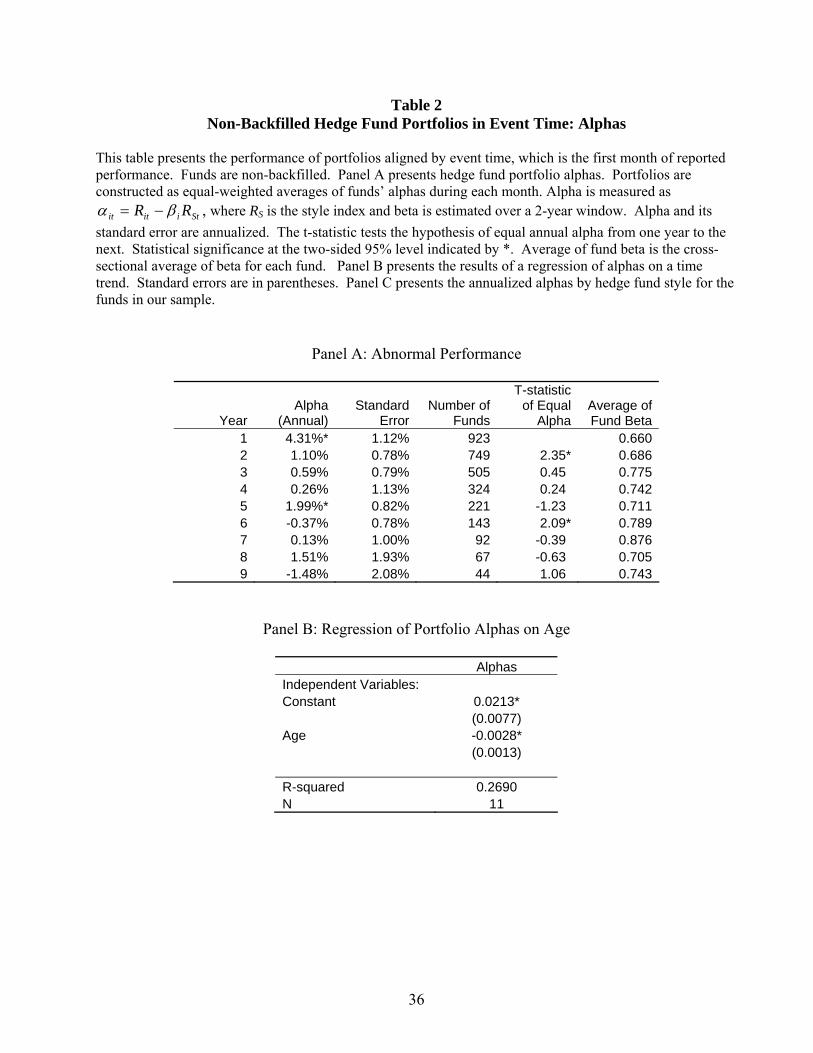
We start by presenting style-adjusted returns for the event-time portfolio. Panel A in Table

2 presents alphas by age, ranging from one to nine years after inception. Panel A shows that first-

year alphas are 4.31%, falling substantially in years two to five, and then varying between positive

and negative values thereafter.17 Standard errors are systematically smaller than in Table 1,

reflecting the increase in power due to the sector adjustment. The test column presents the t-statistic

for the hypothesis of no change in annual return. The first-year drop is statistically significant.

Performance continues to drop in the third and fourth years. To summarize the outperformance, the

average alpha during the first four years is 1.57% per annum, versus 0.36% during the next five

16 We have also examined the Fung and Hsieh (2004) asset-based style (ABS) factors, with betas estimated over the entire period, with similar results. We choose not to report the Fung and Hsieh results because a large number of new funds stop reporting fairly quickly, creating unstable estimates. For example, of our 923 funds, 174 stop reporting within twelve months. 68 of these funds start in 2006 and survive, but cannot report more than twelve months of performance; the rest stop reporting mostly due to failure and liquidation. Estimating Fung and Hsieh seven factor exposures with less than 12 months of data is clearly problematic because we over-fit alphas. On the other hand, dropping these funds results in the elimination of almost 20% of our sample. Nonetheless, when we drop funds with fewer than 12 months of performance, we find results based on the Fung and Hsieh factors that are similar to the results reported based on style indices. 17 To address concerns that there may be some residual backfill bias in our results, we have also examined the funds for which there is no backfill at all because they are added to TASS within 30 days of their first performance report. There are initially 243 such funds. The patterns we describe for the full no backfill sample are similar for this sample as well, but with less statistical power due to the smaller number of funds. In the first year in event time, the average alpha is somewhat smaller at 2.31% with a standard error of 1.19%.

19

years. Emerging managers, narrowly defined as having a maximum life of two years, generate an

abnormal performance of 2.71% per annum relative to 0.38% later. This difference is statistically

and economically significant.

The last column reports the typical fund beta, taken as the arithmetic average of this risk

measure across all the funds in this group. Average betas are around 0.7 relative to the style

indices. This beta differs from unity because the typical fund may not be perfectly correlated with

the style factor (e.g., the manager has new ideas), or may not have the same leverage or volatility.18

Panel B presents results from a regression of portfolio alphas on a time trend. The time

trend is negative and statistically significant. Thus, emerging managers display significantly better

performance during their initial years. Each additional year of age decreases performance (alpha)

by 28 basis points, on average.

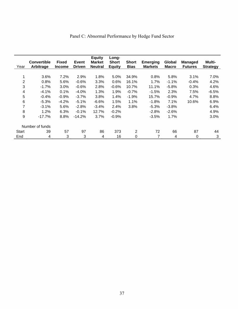
Panel C presents alphas in event time decomposed by hedge fund sector or style. We assign

each of our hedge funds to one of ten sectors and form a portfolio of the hedge funds in that sector.

Panel C shows that the results are not driven by one sector only. Most sectors display a decline in

alphas in event time. This analysis, however, is only suggestive because, relative to Panel A, the

number of funds is perforce smaller for each category and in addition shrinks very quickly in event

time, which creates more variability in the average alphas.

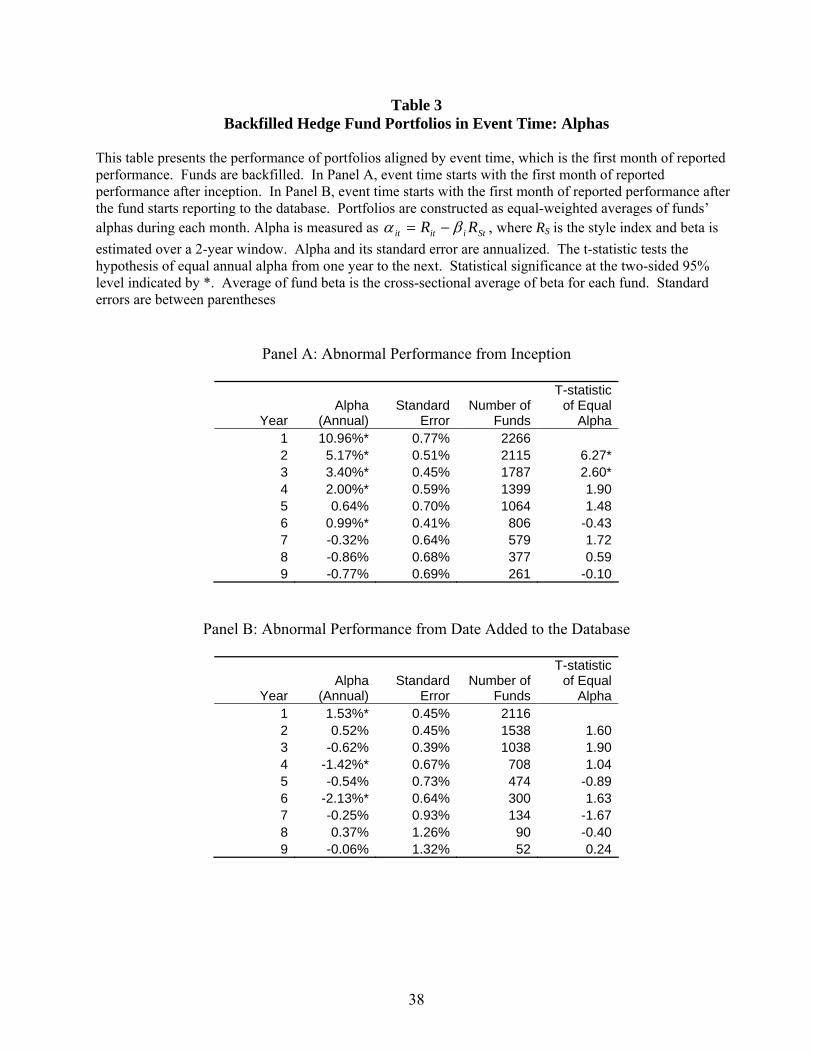
Table 3 presents alphas in event time for the backfilled funds. Panel A presents annual

alphas from the first reported performance after inception. This sample fully incorporates all of the

backfilled data. Not surprisingly, alphas are large but decreasing for the first four years of

inception. To see how much of this performance is due to firms backfilling positive returns, we

reexamine our backfilled sample by truncating all monthly return observations prior to the fund

20

starting to report performance to the database. Since the database reports the date that the fund was

added to the database, we treat all monthly return observations prior to this date as backfilled and

eliminate them. We then compute alphas for the remaining (non-backfilled) observations in event

time, where the event is the fund being added to the database. These results are presented in Panel

B of Table 3. The alphas plummet relative to those in Panel A. Interestingly, alphas are also lower

than for the purely non-backfilled funds in Table 2.

Figure 1 displays the cumulative alphas aligned by event time for our non-backfilled sample.

The initial performance is very strong, then tapers off as the fund ages. Note that the performance

in the first year is not driven by the first three months alone, which should dispel concerns about the

remaining 82-day median period between the performance start date and the date added to the

database. Also note that the beginning of the line is rather smooth, due to the large number of funds

in the series. Towards the end, however, the line is much more irregular. This reflects the greater

standard error due to the fact that the portfolio is less well diversified because it includes a smaller

number of funds. Overall, the figure indicates that performance in the initial few years is better than

average. One point worth noting is that emerging funds are open to investors, whereas many

established funds (including those in the indices) that have performed well are not open to investors.

Thus, in the space of investable funds, emerging funds are likely to be even better performers

relative to established funds.

The figure also displays the cumulative alphas for backfilled funds. The vertical difference

between the two top lines (backfilled versus non-backfilled funds) indicates that the backfill bias is

very substantial. For example, the vertical difference between the two lines after four years is about

18 There does appear to be some tendency for beta to increase over time, which parallels the decrease in alpha. This is in part due to the negative correlation between alpha and beta due to the overlap in estimation period. Because style indices tend to have positive returns, if beta is underestimated, this will lead to an overestimation of alpha.

21

15%, which translates into a bias of about 4% per year. This comparison controls for the age of the

fund, using the non-backfilled funds as a reference.

Alternatively, we could also compare the performance of backfilled funds at different points

in time. The third line in Figure 1 plots the cumulative alphas for the funds from our backfilled

sample starting on the first date of reporting to TASS. In other words, these are the non-backfilled

observations from our sample of backfilled funds. For the first four years, the cumulative alpha is

essentially zero. Comparing the backfilled funds to the backfilled funds without the backfilled

observations, the vertical difference between the two lines after four years is about 21.5%, which

translates into a bias of almost 5.4% per year. Hence, a portfolio of backfilled funds that includes

the backfilled period gives a totally unrealistic view of the performance of emerging managers.

In addition, we can now evaluate the standard practice of discarding the first two years of

the sample to account for backfill bias. Figure 2 compares the cumulative performance of our non-

backfilled sample starting in year 3 to that of the backfilled sample. Without bias, the two lines

should be comparable to each other. In fact, the backfilled sample displays persistently higher

performance than the non-backfilled sample. This is because 37% of funds still have backfilled

numbers even after truncating the first two years. Over the next three years, the difference amounts

to about 3%, which translates into a bias of about 1% per year. Thus, the usual practice of

truncating the first two years is insufficient to purge the backfill bias. The key message here,

however, is that even after carefully controlling for backfill bias, emerging funds perform well in

the first two years of life. This (true) effect is typically missed in hedge fund research when the first

two years of performance is truncated.

One possibility that could explain the difference in the performance of the non-backfilled

versus the backfilled sample is differences in management or incentive fees. It turns out that this is

not the case. For the non-backfilled sample, the average management and incentive fees are 1.50%

22

and 19.65%, versus 1.43% and 19.63% for the backfilled sample. Of course, effective fees can

differ from the stated fees, which are the ones reported to the database and used to compute net

returns. In particular, early investors in emerging managers may be able to get a fee break, which

makes returns for emerging managers even more attractive for early investors than those reported

here.

B. Performance Persistence

These results suggest that emerging managers perform better during their earlier years, on

average. An interesting question is whether these results are driven by a subsample of managers.

To check whether specific managers that have performed well continue to perform well, we

examine whether performance is persistent in the cross-section of emerging managers. We address

this question in two ways.

First, Table 4, Panel A presents the results from a regression of:

ititit bb εαα ++= −110 (3)

where α is the abnormal return as defined in Equation (2). This is a conventional regression

approach where we simply ask whether future abnormal returns are associated with past abnormal

returns. The regression is performed year-by-year in event time. Funds with at least two monthly

observations are kept in the year t sample, so there is very little look-ahead bias. We start by

examining the association between year 2 abnormal returns and year 1 abnormal returns and then

move forward in time. For years 2 and 3, the coefficient on the previous year’s alpha is

approximately 0.30, and is significant. For the remaining years (with the exception of year 8), the

coefficient on the prior year’s alpha is insignificant. Thus, we find a high degree of performance

persistence from years 1 to 2 and years 2 to 3 for emerging managers. After year 3, when the

managers are arguably no longer emerging, we do not find evidence of performance persistence.

23

These results should be interpreted with caution, however, because the regression uses alphas with

substantial estimation error as independent variables. Carpenter and Lynch (1999) provide a

detailed study of the statistical efficiency and power for various measures of performance

persistence and show that this type of test can be unreliable.

This is why we also use a second methodology recommended by Carpenter and Lynch

(1999). In the absence of survivorship bias, which is appropriate in our context because we include

graveyard funds, they recommend forming portfolios of funds based on performance deciles.

Grouping decreases estimation error in the performance measures. Due to the smaller number of

hedge funds relative to mutual funds, we choose to form quintiles instead. We use a one year

ranking period and a one year evaluation period. In event year t-1, we form five portfolios based on

average fund alphas sorted into quintiles. The highest average alphas are in Q5 and the lowest are

in Q1. In year t, we calculate average annual alphas for each of the five portfolios. Partial

observations for funds that disappear during that year are kept in the sample, so there is no look-

ahead bias. We then take the difference between the average annual alpha for Q5 and Q1 and test

whether the difference is statistically significant.

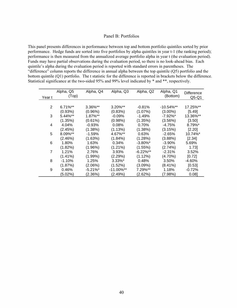
The results are presented in Panel B of Table 4. The differences between Q5 and Q1 are

large in magnitude and statistically significant in years 2 through 5, with values of 17.2%, 13.4%,

8.8%, and 10.7%, respectively.19 These spreads are much larger than the 5.8% spread for all large

funds (assets under management greater than $20 million) in all years reported by Kosowski, Naik,

and Teo (2007), using a Bayesian analysis. However, the spreads from year 6 on are smaller,

consistent with the previous performance persistence results being driven by emerging funds.

Moreover, Kosowski, Naik, and Teo (2007), along with most previous literature, eliminate the first

24

12 months of returns to control for backfill. This is precisely the period for which we find the

results that are largest in magnitude (17.2%). Indeed, when we take a weighted average of the top-

bottom quintile difference across all years, where the weights are the number of funds, we find that

the average difference is 11.99%. Of this, the year 2 difference (based on the year 1 ranking)

accounts for 6.05%. Eliminating the first year, we find that the remainder, 5.94%, is quite similar to

the 5.8% found by Kosowski, Naik, and Teo, although their sample and estimation procedure is

quite a bit different than ours.

In sum, we find performance persistence all the way to year 5.20 Thereafter, the spread falls

sharply. In addition, performance persistence occurs in both the top quintile and the bottom

quintile, with large positive alphas for the top quintile through year 5 and large negative alphas for

the bottom quintile through year 6. This finding is important because performance persistence for

poorly performing funds can happen mechanically—poor performance causes redemptions, which

force liquidation of fund holdings generating additional poor performance. Overall, we conclude

that not only does the average emerging manager perform well for the first few years, but the

specific emerging managers (grouped into portfolios) that perform well in the first few years seem

to continue to do so.

19 The t statistics assume independence across portfolios. This is a reasonable assumption because sorting by event time mixes calendar months, as in conventional event studies. Indeed the results are similar when using the time-series of the differences in portfolio returns to construct the t statistics. 20 One concern with this result is that our alphas are calculated in-sample using betas estimated over two years. It is possible that this induces a spurious autocorrelation in the alphas. We address this in two ways. First, simulation results (not reported) show that any induced autocorrelation is small in magnitude and cannot account for the high degree of persistence we find. Second, we re-examine our results using betas estimated over one year and with alphas calculated out-of-sample. All of the results are quite similar, suggesting that the two-year beta estimation horizon cannot account for any of our results. These results are available upon request.

25

C. Controlling for Size

The evidence of better performance during the early years of a fund’s life that we previously

documented can be attributed to a number of explanations related to incentive effects, as previously

discussed. Another explanation, however, could be size. It could very well be that outperformance

is due to the small size of the fund instead of its age. Size is measured by assets under management

(AUM) for each fund, as reported by TASS. To check this hypothesis, we evaluate the performance

of funds sorted by size quintiles. In this experiment, we sort funds using AUM at the time of

inception. For consistency in reporting, AUM is reported in 2006 dollars adjusted for inflation.

We sort funds by year of inception rather than pooling all of the funds and forming quintiles.

This is because the average size of new funds has increased significantly over time. Therefore, if

we pooled all of the funds to form quintiles, the funds in the largest quintile would predominantly

come from 2006 and our largest quintile would disappear after a year. So, we form quintiles of

funds starting in 1996, quintiles of funds starting in 1997, and so on. We then aggregate all of the

funds in the smallest quintiles, all of the funds in the second quintiles, etc., to create the final five

quintiles.21

Next, we run the analysis in event time, keeping each fund in the same quintile. In other

words, funds may grow or shrink over time, but their assigned quintile does not change. This

analysis can be viewed as choosing funds strictly based on size when they start. This answers the

question of whether funds that are small initially outperform or not. A disadvantage of this sorting

method is that it does not ensure a continuously balanced allocation to quintiles. Each quintile

contains 20% of the 923 funds during the first month. Over event time, however, the number of

funds decreases sharply and the allocation of funds to quintiles becomes unbalanced as funds

21 For reference, we also report the average AUM in 2006 dollars for the final five quintiles.

26

disappear. After 10 years, for instance, there are no remaining funds in the smallest quintile. This

effect also shows up as larger standard errors.

The results are displayed in Table 5. The table does not show a uniform size effect in the

alphas. The last column presents the average alpha and standard error by quintile over the first nine

years. The average alpha for the smallest quintile is −1.96% and for the largest quintile is +0.01%.

The bottom two rows of Table 5 present the results of a joint test of equality of alphas across the

five quintiles. Only for the first year do we come close to rejecting the hypothesis of equality of

alphas, with a p-value of 0.10. In general, variations across quintiles are less important than

variations across years. In other words, picking a manager by age is more informative than by size.

To the extent that there are significant patterns due to size effects, larger managers seem to

do better, especially in the first year or two of existence. This is contrary to the hypothesis that

small managers should outperform others. One possible explanation is that the funds in our sample

are rather small at inception. Funds in the smallest quintile have average assets under management

of less than $1 million. Only in the largest quintile do funds start with average AUM in excess of

$50 million, which, incidentally, is the cutoff size for inclusion in hedge fund style indices. Given

this small size, emerging funds are unlikely to suffer from diseconomies of scale. If anything, they

may benefit from greater economies of scale, such as decreased trading costs and better access to

information. Put differently, the relationship between performance and size is probably not linear,

with very small funds underperforming because of economies of scale and very large funds

underperforming because of diseconomies of scale. In addition and not surprisingly, smaller

managers at inception seem to exit at a more rapid rate over time than larger managers. This is

consistent with the hypothesis that investors can identify managers with greater skill and provide

them with more funds. Thus, investors seem to be able to successfully screen new managers.

27

C. Cohort by Calendar Year Analysis

To further examine the effects of age and size, we provide an alternative time alignment

classification based on a cohort by calendar year analysis. Here we keep track of the calendar year

in which the fund is started so that we can reform size portfolios for funds started in a specific year

(e.g., 1996) in every subsequent January. Before examining size, we present aggregate statistics on

raw returns and alphas over time for the cohort by calendar year time alignment in Table 6, Panel A.

First-year returns are computed by averaging returns in 1996 for funds started in 1996 with returns

in 1997 from funds started in 1997, and so on. Second-year returns are computed by averaging

returns in 1997 for funds started in 1996 with returns in 1998 for funds started in 1997, and so on.

The rest of the returns are calculated in analogous fashion.

The results in Table 6, Panel A, are comparable to those in Tables 1 and 2 with two

exceptions. First-year performance is higher under this method. Also, the portfolio volatility is

systematically higher. This reflects the fact that, at the beginning of the calendar year, there are

fewer funds in these portfolios than in Tables 1 and 2. In particular, there are many fewer funds in

January and February of the first calendar year of existence.22 As previously documented, early

performance tends to be good, so that the months of January and February will tend to have very

strong performance in the first year of existence. When we then average across the months to get

yearly performance, we generate first-year results that seem much better than in the event-time

analysis.

Next, we want to examine more closely the effects we find for age and size in the previous

section. Recall that we found evidence that initial fund performance is strong, especially for larger

managers. Each fund was assigned to a quintile constructed using equal weights, and stayed in the

22 For example, if all funds were to start uniformly during the first year, the number of funds in the December portfolio would be 12 times that in January.

28

same quintile over time. These results, however, could be obscuring an interaction between size

and age. Specifically, our results could be obscuring better performance over time by larger funds

and worse performance by smaller funds. When we form equally-weighted portfolios, we

essentially dilute the strong performance of the larger funds.

To see this, suppose that investors start with diffuse priors about the ability of portfolio

managers and the distribution of initial fund sizes is random. As in the Berk and Green (2004)

model, now assume that a fund performing well early will attract investor inflows that increase its

assets under management; at least for a while, the fund continues to perform well. Conversely,

firms that initially perform badly show a decrease in assets and continue to perform badly. Under

these conditions, equally-weighted portfolios will overweight poorly performing small funds and

underweight the strong performance of large funds. This effect is not captured by the design of the

previous section because funds were frozen into the quintiles they occupied at inception. No

allowance was made for the possibility that funds might grow or shrink over time based on their

performance.

To address these concerns, we want to allow the fund classification and size portfolios to

change over time. In order to do so, we re-sort all funds at the beginning of each subsequent year

into size quintiles.23 This method also ensures that the quintiles are equally balanced throughout

time, which is not the case with the event time method where we left the quintiles frozen over time.

Panel B in Table 6 displays alphas from size quintile portfolios where the portfolios are

reformed every year. In general, the results are similar to those in Table 5. For the most part,

differences across size portfolios are not statistically significant. Even so, large funds seem to

perform better than smaller funds. The smallest funds do very well in the first year, after which

29

performance worsens significantly. Compared to the fixed quintiles in Table 5, large funds in the

top quintile in Table 6 perform better. Thus, while there is some evidence of a size effect—large

funds do better—there is also evidence of an age effect—younger funds do better and then

performance deteriorates.

To examine these competing effects, Panel C presents the results of a regression of portfolio

alphas on both age and size quintiles. We find that the time trend is negative and significant, while

the effect of size is positive but insignificant. Controlling for size, each additional year of age

decreases performance (alpha) by 48 basis points, on average. This confirms that, even after

controlling for possible performance persistence due to size, emerging hedge fund managers do

perform better than their older counterparts.

V. Conclusions

While recent research has analyzed various facets of hedge fund performance, none has

focused on emerging managers. This is a particularly interesting category given the incentive

features of the hedge fund industry. Emerging managers have particularly strong financial

incentives to create performance and may be more nimble than established ones.

This paper provides the first systematic analysis of performance patterns for emerging hedge

fund managers. This task is complicated by the practice of backfilling hedge fund databases, which

may involve the selective reporting of ex post returns going back to the start of performance.

Because reporting is voluntary, managers are more likely to report good results rather than bad

results, leading to a backfill bias in performance evaluation that is particularly severe for emerging

managers. This study controls for backfill and survivorship bias. We also find that the usual

23 Performing this analysis in event time is problematic because resorting by size every 12 months without regard to calendar year mixes funds from different years, and we know that there is a calendar time component to fund size (e.g.,

30

practice in empirical research of eliminating the first 12 or 24 months of the sample is insufficient to

purge the backfill bias.

We make several contributions to the literature. First, we examine how hedge funds

perform over time and what role age plays in performance. Prior work which pools hedge funds

over time or examines hedge fund performance cross-sectionally misses the role of age. For

example, if new hedge funds do well initially, and many new hedge funds are started every year,

then one might (mistakenly) conclude that hedge funds do well over time. Our cohort analysis and

event time analysis allow us to show that the performance of new hedge funds does deteriorate over

time.

Second, we specifically examine how new or emerging managers perform. This is

interesting not only because new managers have strong incentives to perform well, but also because

they are open to new investors whereas older, strongly-performing hedge funds may not be. Prior

research has typically ignored emerging hedge funds in an attempt to control for the severe

problems with backfill bias. We take a more rigorous approach to eliminating backfilled funds to

examine the performance of emerging managers.

Third, we find strong evidence of outperformance during the first two or three years of

existence. Emerging managers, narrowly defined as having a maximum life of two years, generate

an abnormal performance of 2.3% relative to the later years. This difference is statistically and

economically significant. This effect does not seem to have a simple relationship with size. Large

emerging managers do better, but the relationship is not uniform. Controlling for size, a simple

linear regression of abnormal returns on time reveals that each additional year of age decreases

performance by 48 basis points, on average. In addition, we find strong evidence that, for

individual managers, early performance is quite persistent. We find performance is persistent for up

the average size of a new fund increases over time).

31

to five years for emerging managers. Thereafter, performance persistence fades away, along with

the outperformance we also document. Thus, as predicted by theory, emerging managers tend to

add value relative to their peers.

32

REFERENCES

Ackermann, C., R. McEnally, and D. Ravenscraft, 1999, “The Performance of Hedge Funds: Risk,

Return, and Incentives,” Journal of Finance 54, 833—874.

Agarwal, Vikas, Naveen Daniel, and Narayan Naik, 2007, “Role of managerial incentives and

discretion in hedge fund performance,” Working Paper, London Business School.

Agarwal, Vikas and Narayan Naik, 2000, “Multi-Period Performance Persistence Analysis of

Hedge Funds,” Journal of Financial and Quantitative Analysis 35 (3), 327—342.

Aggarwal, Rajesh K., Galin Georgiev, and Jake Pinato, 2007, “Detecting Performance Persistence

in Fund Managers: Book Benchmark Alpha Analysis,” Journal of Portfolio Management

(Winter), 110—119.

Allen, Gregory, 2007, “Does Size Matter?” Journal of Portfolio Management (Spring), 57—62.

Baquero, G., J. Ter Horst, and M. Verbeek, 2005, “Survival, Look-Ahead Bias and the Persistence

in Hedge Fund Performance,” Journal of Financial and Quantitative Analysis 40, 493—517.

Berk, Jonathan and Richard Green, 2004, “Mutual Fund Flows and Performance in Rational

Markets,” Journal of Political Economy 112, 1269—1294.

Boyson, Nicole, 2005, “Another look at career concerns: a study of hedge fund managers,”

Working Paper, Northeastern University (November version).

Brown, Steve, William Goetzmann, and Roger Ibbotson, 1999, “Offshore Hedge Funds: Survival

and Performance 1989-1995,” Journal of Business 72, 91—118.

Brown, Steve, William Goetzmann, and J. Park, 2001, “Careers and Survival: Competition and Risk

in the Hedge Fund and CTA Industry,” Journal of Finance 56, 1869—1886.

Carhart, Mark, Jennifer Carpenter, Anthony Lynch, and David Musto, 2002, “Mutual Fund

Survivorship,” Review of Financial Studies 15, 1439—1463.

33

Carhart, Mark, 1997, “On Persistence in Mutual Fund performance,” Journal of Finance 52 (1),

57—82.

Carpenter, Jennifer and Anthony Lynch, 1999, “Survivorship bias and attribution effects in

measures of performance persistence,” Journal of Financial Economics 54, 337-374.

Chen, J. S., H. Hong, M. Huang, and J. Kubik, 2004, “Does Fund Size Erode Mutual Fund

Performance? The Role of Liquidity and Organization,” American Economic Review 94(5),

1276—1302.

Chevalier, Judith and Glenn Ellison, 1997, “Risk-taking by mutual funds as a response to

incentives,” Journal of Political Economy 105(6), 1167—1200.

Chevalier, Judith and Glenn Ellison, 1999, “Career concerns of mutual fund managers,” Quarterly

Journal of Economics 114(2), 389—432.

Evans, Richard, 2007, “The Incubation Bias,” Working Paper, University of Virginia.

Fung, William and David. Hsieh, 1997, “Empirical characteristics of dynamic trading strategies:

The case of hedge funds,” Review of Financial Studies 10, 275—302.

Fung, William and David Hsieh, 2001, “The Risk in Hedge Fund Strategies: Theory and Evidence

from Trend Followers,” Review of Financial Studies 12, 313—341.

Fund, William and David Hsieh, 2004, “Hedge Fund Benchmarks: A Risk-Based Approach,”

Financial Analysts Journal 60, 65—80.

Getmansky, Mila, Andrew Lo, and Igor Makarov, 2004, “An econometric model of serial

correlation and illiquidity in hedge fund returns,” Journal of Financial Economics 74, 529—

609.

Goetzmann, William, Jon Ingersoll, and Steve Ross, 2003, “High-Water Marks and Hedge Fund

Management Contracts,” Journal of Finance 58, 1685—1717.

34

Grinblatt, M., and S. Titman, 1989, “Mutual Fund Performance: An Analysis of Quarterly Portfolio

Holdings,” Journal of Business 62, 393-416.

Howell, Michael, 2001, “The Young Ones,” AIMA Newsletter, June.

Jagannathan, R. A. Malakhov, and D. Novikov, 2007, “Do Hot Hands Persist Among Hedge Fund

Managers? An Empirical Evaluation,” Working Paper, Northwestern University.

Jensen, M. and W. Meckling, 1976, “Theory and the firm: Managerial behavior, agency costs and

ownership structure,” Journal of Financial Economics 3, 305—360.

Jones, Meredith, 2007, “Examination of Fund Age and Size and its Impact on Hedge Fund

Performance,” Derivatives Use, Trading and Regulation 12(4), 342—350.

Kosowski, Robert, Narayan Naik, and Melvyn Teo, 2007, “Do hedge funds deliver alpha? A

Bayesian and bootstrap analysis,” Journal of Financial Economics 84, 229-264.

Liang, Bing, 2000, “Hedge Funds: The Living and the Dead,” Journal of Financial and

Quantitative Analysis 35, 309—326.

Malkiel, Burton and Anatu Saha, 2005, “Hedge Funds: Risk and Return,” Financial Analysts

Journal 61, 80—88.

Massa, Massimo and Rajdeep Patgiri, 2006, “Incentives and Mutual Fund Performance: Higher

Performance or Just Higher Risk Taking?” Working Paper, INSEAD.

Pérold, André and Robert Salomon, 1991, “The Right Amount of Assets under Management,”

Financial Analysts Journal 47(3), 31-39.

Wermers, R., 2000, “Mutual Fund Performance: An Empirical Decomposition into Stock-Picking

Talent, Style, Transaction Costs, and Expenses,” Journal of Finance 55, 1655-1695.

35

Table 1 Hedge Fund Portfolios in Event Time: Raw Returns

This table presents the performance of portfolios aligned by event time, which is the first month of reported performance. Portfolios are constructed as equal-weighted averages of fund raw returns during each month. Returns are then grouped by year, i.e., first twelve months for year 1 and so on. Annualized volatility is reported for each year, from the portfolio time series. The t-statistic tests the hypothesis of equal annual return from one year to the next. Statistical significance at the two-sided 95% level indicated by *. Average of fund volatility is the cross-sectional average of annualized volatility for each fund over 12 months. Panel A presents results for funds with no backfill, i.e., with the inception date very close to the date first reported to the database. Panel B presents results for funds with backfill, i.e., which do not satisfy the previous definition. Number of funds is at the start of each cohort year.

Panel A: Funds With No Backfill

Cohort Year

Raw Returns (Annual)

Annualized Volatility

(Portfolio)Number

of Funds

T-statistic of Equal

Return

Average of Fund

Volatility 1 12.16% 1.27% 923 12.73% 2 7.99% 0.82% 749 2.76* 12.52% 3 7.30% 1.26% 505 0.46* 12.01% 4 8.32% 1.07% 324 -0.61* 11.19% 5 8.90% 1.12% 221 -0.38* 9.93% 6 6.69% 1.03% 143 1.45* 9.78% 7 11.06% 1.54% 92 -2.36* 8.97% 8 9.97% 1.95% 67 0.44* 8.77% 9 11.83% 2.88% 44 -0.53* 10.13%

Panel B: Backfilled Funds

Cohort Year

Raw Returns (Annual)

Annualized Volatility

(Portfolio)Number

of Funds

T-statistic of Equal

Return

Average of Fund

Volatility 1 18.60% 0.62% 2267 14.22% 2 12.41% 0.99% 2116 5.28* 13.19% 3 11.84% 1.21% 1788 0.36* 12.58% 4 10.72% 0.64% 1400 0.82* 11.90% 5 8.26% 1.32% 1064 1.68* 11.52% 6 9.13% 0.92% 806 -0.54* 10.58% 7 11.72% 1.51% 579 -1.46* 10.28% 8 11.51% 1.54% 377 0.09* 9.97% 9 11.34% 1.39% 261 0.08* 9.63%

36

Table 2 Non-Backfilled Hedge Fund Portfolios in Event Time: Alphas

This table presents the performance of portfolios aligned by event time, which is the first month of reported performance. Funds are non-backfilled. Panel A presents hedge fund portfolio alphas. Portfolios are constructed as equal-weighted averages of funds’ alphas during each month. Alpha is measured as

Stiitit RR βα −= , where RS is the style index and beta is estimated over a 2-year window. Alpha and its standard error are annualized. The t-statistic tests the hypothesis of equal annual alpha from one year to the next. Statistical significance at the two-sided 95% level indicated by *. Average of fund beta is the cross-sectional average of beta for each fund. Panel B presents the results of a regression of alphas on a time trend. Standard errors are in parentheses. Panel C presents the annualized alphas by hedge fund style for the funds in our sample.

Panel A: Abnormal Performance

Year Alpha

(Annual)Standard

ErrorNumber of

Funds

T-statistic of Equal

Alpha

Average of Fund Beta

1 4.31%* 1.12% 923 0.660 2 1.10% 0.78% 749 2.35* 0.686 3 0.59% 0.79% 505 0.45* 0.775 4 0.26% 1.13% 324 0.24* 0.742 5 1.99%* 0.82% 221 -1.23* 0.711 6 -0.37% 0.78% 143 2.09* 0.789 7 0.13% 1.00% 92 -0.39* 0.876 8 1.51% 1.93% 67 -0.63* 0.705 9 -1.48% 2.08% 44 1.06* 0.743

Panel B: Regression of Portfolio Alphas on Age

Alphas Independent Variables: Constant 0.0213* (0.0077) Age -0.0028* (0.0013) R-squared 0.2690 N 11

37

Panel C: Abnormal Performance by Hedge Fund Sector

Year Convertible Arbitrage

Fixed Income

Event Driven

Equity Market Neutral

Long-Short Equity

Short Bias

Emerging Markets

Global Macro

Managed Futures

Multi-Strategy

1 3.6% 7.2% 2.9% 1.8% 5.0% 34.9% 0.8% 5.8% 3.1% 7.0%2 0.8% 5.6% -0.6% 3.3% 0.6% 16.1% 1.7% -1.1% -0.4% 4.2%3 -1.7% 3.0% -0.6% 2.8% -0.6% 10.7% 11.1% -5.8% 0.3% 4.6%4 -4.1% 0.1% -4.0% 1.3% 1.9% -0.7% -1.5% 2.3% 7.5% -6.5%5 -0.4% -0.9% -3.7% 3.8% 1.4% -1.9% 15.7% -0.9% 4.7% 8.8%6 -5.3% -4.2% -5.1% -6.6% 1.5% 1.1% -1.8% 7.1% 10.6% 6.9%7 -3.1% 5.6% -2.8% -3.4% 2.4% 3.8% -5.3% -3.8% 6.4%8 1.2% 6.3% -0.1% 12.7% -0.2% -2.8% -2.6% 4.9%9 -17.7% 8.8% -14.2% 3.7% -0.9% -3.5% 1.7% 3.0%

Number of funds

Start 39 57 97 86 373 2 72 66 87 44End 4 3 3 4 16 0 7 4 0 3

38

Table 3 Backfilled Hedge Fund Portfolios in Event Time: Alphas

This table presents the performance of portfolios aligned by event time, which is the first month of reported performance. Funds are backfilled. In Panel A, event time starts with the first month of reported performance after inception. In Panel B, event time starts with the first month of reported performance after the fund starts reporting to the database. Portfolios are constructed as equal-weighted averages of funds’ alphas during each month. Alpha is measured as Stiitit RR βα −= , where RS is the style index and beta is estimated over a 2-year window. Alpha and its standard error are annualized. The t-statistic tests the hypothesis of equal annual alpha from one year to the next. Statistical significance at the two-sided 95% level indicated by *. Average of fund beta is the cross-sectional average of beta for each fund. Standard errors are between parentheses

Panel A: Abnormal Performance from Inception

Year Alpha

(Annual)Standard

ErrorNumber of

Funds

T-statistic of Equal

Alpha 1 10.96%* 0.77% 2266 2 5.17%* 0.51% 2115 6.27* 3 3.40%* 0.45% 1787 2.60* 4 2.00%* 0.59% 1399 1.90 5 0.64% 0.70% 1064 1.48 6 0.99%* 0.41% 806 -0.43 7 -0.32% 0.64% 579 1.72 8 -0.86% 0.68% 377 0.59 9 -0.77% 0.69% 261 -0.10

Panel B: Abnormal Performance from Date Added to the Database

Year Alpha

(Annual)Standard

ErrorNumber of

Funds

T-statistic of Equal

Alpha 1 1.53%* 0.45% 2116 2 0.52% 0.45% 1538 1.60 3 -0.62% 0.39% 1038 1.90 4 -1.42%* 0.67% 708 1.04 5 -0.54% 0.73% 474 -0.89 6 -2.13%* 0.64% 300 1.63 7 -0.25% 0.93% 134 -1.67 8 0.37% 1.26% 90 -0.40 9 -0.06% 1.32% 52 0.24

39

Table 4 Performance Persistence in Event Time—Non-Backfilled Hedge Funds

Panel A: Alpha Regressions

This panel presents the results of year-by-year cross-sectional regressions of: .110 itittit bb εαα ++= −− We use the non-backfilled funds. Funds are aligned in event time: the first twelve months of performance are year 1, the second twelve months are year 2, etc. Alpha is measured as Stiitit RR βα −= , where RS is the style index and beta is estimated over a 2-year window. The regression tests for persistence in alphas year to year. The constant is not reported. Statistical significance at the two-sided 95% and 99% level indicated by * and **, respectively.

Year t

Coefficient, Alpha

Year t-1Standard Error

of CoefficientNumber of

Observations

Adj.

R-squared

2 0.297** 0.046 733 0.054 3 0.303** 0.046 491 0.081 4 0.072** 0.061 314 0.001 5 0.114** 0.125 218 -0.000 6 0.077** 0.064 139 0.003 7 0.174** 0.106 88 0.019 8 -0.270** 0.124 65 0.056 9 -0.130** 0.183 43 -0.011

40

Panel B: Portfolios

This panel presents differences in performance between top and bottom portfolio quintiles sorted by prior performance. Hedge funds are sorted into five portfolios by alpha quintiles in year t-1 (the ranking period); performance is then measured from the annualized average portfolio alpha in year t (the evaluation period). Funds may have partial observations during the evaluation period, so there is no look-ahead bias. Each quintile’s alpha during the evaluation period is reported with standard errors in parentheses. The “difference” column reports the difference in annual alpha between the top quintile (Q5) portfolio and the bottom quintile (Q1) portfolio. The t statistic for the difference is reported in brackets below the difference. Statistical significance at the two-sided 95% and 99% level indicated by * and **, respectively.

Year t Alpha, Q5

(Top) Alpha, Q4 Alpha, Q3 Alpha, Q2 Alpha, Q1

(Bottom) Difference

Q5-Q1

2

6.71%** (0.93%)

3.36%** (0.96%)

3.20%** (0.83%)

-0.81% (1.07%)

-10.54%** (3.00%)

17.25%** [5.49]

3

5.44%** (1.35%)

1.87%** (0.61%)

-0.09% (0.98%)

-1.49% (1.35%)

-7.92%* (3.56%)

13.36%** [3.50]

4

4.04% (2.45%)

-0.93% (1.38%)

0.08% (1.13%)

0.70% (1.38%)

-4.75% (3.15%)

8.79%** [2.20]

5

8.09%** (2.46%)

-1.59% (1.63%)

4.67%** (1.84%)

0.63% (1.28%)

-2.65% (3.88%)

10.74%* [2.34]*

6

1.80% (1.82%)

1.63% (1.96%)

0.34% (1.21%)

-3.80%* (1.55%)

-3.90% (2.74%)

5.69%** [1.73]

7

1.21% (1.41%)

2.76% (1.99%)

3.93% (2.29%)

-6.22%** (1.12%)

-2.31% (4.70%)

3.52% [0.72]*

8

-1.10% (1.87%)

1.25% (2.06%)

3.33%* (1.52%)

0.48% (3.09%)

3.50% (8.41%)

-4.60%** [0.53]

9

0.46% (5.02%)

-5.21%* (2.36%)

-11.00%** (2.49%)

7.29%** (2.62%)

1.18% (7.98%)

-0.72%* [0.08]

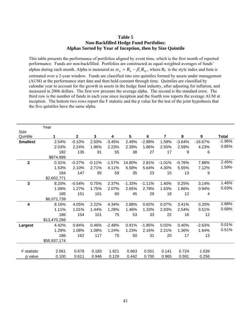
41

Table 5

Non-Backfilled Hedge Fund Portfolios: Alphas Sorted by Year of Inception, then by Size Quintile

This table presents the performance of portfolios aligned by event time, which is the first month of reported performance. Funds are non-backfilled. Portfolios are constructed as equal-weighted averages of funds’ alphas during each month. Alpha is measured as Stiitit RR βα −= , where RS is the style index and beta is estimated over a 2-year window. Funds are classified into size quintiles formed by assets under management (AUM) at the performance start date and then held constant through time. Quintiles are classified by calendar year to account for the growth in assets in the hedge fund industry, after adjusting for inflation, and measured in 2006 dollars. The first row presents the average alpha. The second is the standard error. The third row is the number of funds in each year since inception and the fourth row reports the average AUM at inception. The bottom two rows report the F statistic and the p value for the test of the joint hypothesis that the five quintiles have the same alpha.

Year Size Quintile 1 2 3 4 5 6 7 8 9

Total

Smallest 2.54% -0.10% 2.50% -3.45% 2.49% -2.88% 1.59% -3.64% -16.67% -1.96% 2.03% 2.24% 1.96% 2.23% 2.39% 1.86% 2.55% 2.59% 4.23% 0.85% 182 135 91 55 38 27 17 9 6 $874,989

2 0.31% -0.27% -0.11% -1.57% 14.80% 2.81% -1.01% -0.76% 7.88% 2.45% 1.53% 2.10% 2.71% 4.11% 6.58% 5.64% 4.30% 5.55% 7.12% 1.59% 184 147 95 59 35 23 15 13 9 $2,602,771 3 8.20% -0.54% 0.75% 2.37% -1.33% -1.11% 1.40% 0.25% 3.14% 1.46% 1.09% 1.27% 1.75% 2.07% 2.65% 2.78% 1.63% 1.86% 0.94% 0.63% 185 151 101 60 45 29 18 12 4 $6,072,739 4 8.16% 4.05% 2.22% 4.34% 2.88% 0.62% 0.07% 3.41% 0.20% 2.88%

1.11% 1.01% 1.44% 1.28% 1.46% 1.33% 2.93% 2.54% 3.51% 0.68% 186 154 101 75 53 33 22 16 12 $13,470,266 Largest 4.42% 0.84% 0.46% -2.48% 0.91% -1.85% 0.02% 0.40% -2.63% 0.01% 1.29% 1.08% 1.08% 1.24% 1.23% 2.16% 2.21% 1.36% 1.64% 0.51% 186 162 117 75 50 31 20 17 13 $55,937,174

F statistic 2.061 0.678 0.183 1.921 0.963 0.551 0.141 0.724 1.639p value 0.100 0.611 0.946 0.129 0.442 0.700 0.965 0.591 0.256

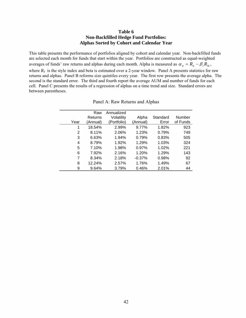
42

Table 6 Non-Backfilled Hedge Fund Portfolios:

Alphas Sorted by Cohort and Calendar Year This table presents the performance of portfolios aligned by cohort and calendar year. Non-backfilled funds are selected each month for funds that start within the year. Portfolios are constructed as equal-weighted averages of funds’ raw returns and alphas during each month. Alpha is measured as Stiitit RR βα −= , where RS is the style index and beta is estimated over a 2-year window. Panel A presents statistics for raw returns and alphas. Panel B reforms size quintiles every year. The first row presents the average alpha. The second is the standard error. The third and fourth report the average AUM and number of funds for each cell. Panel C presents the results of a regression of alphas on a time trend and size. Standard errors are between parentheses.

Panel A: Raw Returns and Alphas

Year

Raw Returns (Annual)

Annualized Volatility

(Portfolio)Alpha

(Annual)Standard

ErrorNumber

of Funds 1 18.54% 2.99% 9.77% 1.82% 923 2 8.11% 2.06% 1.23% 0.79% 749 3 6.63% 1.94% 0.79% 0.83% 505 4 8.79% 1.92% 1.29% 1.03% 324 5 7.10% 1.98% 0.97% 1.02% 221 6 7.92% 2.16% 1.20% 1.29% 143 7 8.34% 2.18% -0.37% 0.98% 92 8 12.24% 2.57% 1.76% 1.49% 67 9 9.64% 3.79% 0.46% 2.01% 44

43

Panel B: Alphas Sorted by Age and Size (Size Quintiles Reformed Every Year)

Panel C: Regression of Portfolio Alphas on Age and Size Quintile

Calendar Year

Alphas Independent Variables: Constant 0.0293* (0.0132) Age -0.0048* (0.0018) Size 0.0037 (0.0040) R-squared 0.1030 N 55

Cohort Size Quintile 1 2 3 4 5 6 7 8 9 TotalSmallest 13.70% -4.15% -1.89% -1.25% -3.68% -4.41% -3.85% 9.87% -9.03% -0.52% 3.75% 2.16% 2.54% 4.12% 3.75% 3.62% 2.79% 5.86% 5.39% 1.32% 184 161 114 72 49 32 20 14 10 2 3.13% 2.35% 1.62% 4.76% 1.73% 0.81% -0.44% -0.26% 3.42% 1.90% 3.36% 1.53% 2.18% 2.03% 2.16% 2.09% 2.33% 3.33% 5.64% 0.99% 185 162 116 74 49 34 22 15 11 3 6.21% 1.53% -0.31% 3.32% -0.48% -0.06% 0.19% -2.46% 0.41% 0.93% 1.47% 1.51% 1.57% 1.59% 2.23% 1.59% 1.67% 1.70% 1.73% 0.56% 185 161 114 74 51 32 20 14 11 4 14.56% 2.93% 2.75% -0.75% 4.85% 2.97% 1.06% 1.03% 4.00% 3.71% 3.17% 1.14% 1.19% 1.27% 2.14% 3.16% 1.30% 1.80% 2.17% 0.69% 184 162 114 74 49 32 22 15 11 Largest 7.16% 2.79% 1.72% -0.36% 0.53% 4.64% 0.10% 1.41% 0.79% 2.09% 2.19% 1.04% 1.00% 0.92% 1.15% 0.98% 1.27% 1.25% 2.46% 0.49% 184 161 114 72 49 32 20 14 10 F statistic 1.701 1.083 0.494 1.588 0.383 1.742 0.259 0.869 3.472*p value 0.164 0.376 0.740 0.199 0.819 0.172 0.901 0.505 0.050

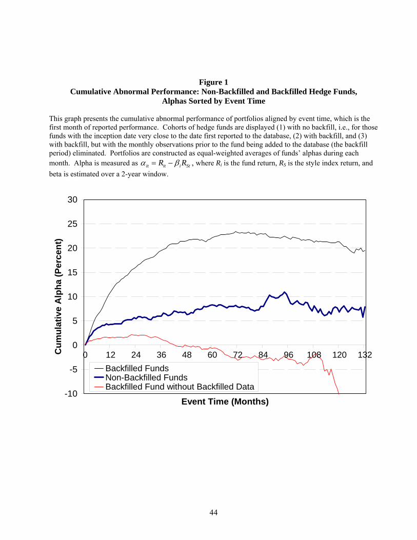
44

Figure 1

Cumulative Abnormal Performance: Non-Backfilled and Backfilled Hedge Funds, Alphas Sorted by Event Time

This graph presents the cumulative abnormal performance of portfolios aligned by event time, which is the first month of reported performance. Cohorts of hedge funds are displayed (1) with no backfill, i.e., for those funds with the inception date very close to the date first reported to the database, (2) with backfill, and (3) with backfill, but with the monthly observations prior to the fund being added to the database (the backfill period) eliminated. Portfolios are constructed as equal-weighted averages of funds’ alphas during each month. Alpha is measured as Stiitit RR βα −= , where Ri is the fund return, RS is the style index return, and beta is estimated over a 2-year window.

-10

-5

0

5

10

15

20

25

30

0 12 24 36 48 60 72 84 96 108 120 132

Event Time (Months)

Cum

ulat

ive

Alp

ha (P

erce

nt)

Backfilled FundsNon-Backfilled FundsBackfilled Fund without Backfilled Data

45

Figure 2 Cumulative Abnormal Performance: Non-Backfilled and Backfilled Hedge Funds,

Alphas Sorted by Event Time Eliminating the First 24 Months This graph presents the cumulative abnormal performance of portfolios aligned by event time, which is the first month of reported performance. Cohorts of hedge funds are displayed (1) with no backfill, i.e., for those funds with the inception date very close to the date first reported to the database, and (2) with backfill. Cohorts are shown after elimination of the first 24 months of alphas. Portfolios are constructed as equal-weighted averages of funds’ alphas during each month. Alpha is measured as Stiitit RR βα −= , where Ri is the fund return, RS is the style index return, and beta is estimated over a 2-year window.

0

5

10

15

20

25

0 12 24 36 48 60 72 84 96 108 120 132

Event Time (Months)

Cum

ulat

ive

Alp

ha (P

erce

nt)

Backfilled Funds

Non-Backfilled Funds