THE PERVERSE EFFECTS OF PARTIAL LABOUR … · THE PERVERSE EFFECTS OF PARTIAL LABOUR MARKET REFORM: FIXED-TERM CONTRACTS ... The main effect may be high turnover in ... productivity

THE PERVERSE EFFECTS OF PARTIAL LABOUR MARKETREFORM: FIXED-TERM CONTRACTS IN FRANCE*

Olivier Blanchard and Augustin Landier

We argue that the effects of a partial reform of employment protection by allowing firms to hireworkers on fixed-term contracts may be perverse. The main effect may be high turnover inentry-level jobs, leading to higher, not lower, unemployment. Even if unemployment falls,workers may be worse off, going through many spells of unemployment and entry-level jobs,before obtaining a regular job. Considering French data for young workers since the early1980s, we conclude that the reforms have substantially increased turnover, without a substantialreduction in unemployment duration. If anything, the effect on their welfare appears to havebeen negative.

There is now substantial evidence that high employment protection leads to asclerotic labour market, with low separation rates but long unemployment dura-tion.1 While this sclerosis may not lead to high unemployment – because of theopposite effects of low flows and high duration on the unemployment rate – it islikely to lead to lower productivity, lower output and to lower welfare.

Broad reductions in employment protection, however, run into strong politicalopposition. The reason is simple: those who are currently protected see themselvesas having more to lose than to gain from such a reduction. For this reason, gov-ernments have either done little, or have tried to reform at the margin, allowingfor reduced protection, but only for (some) new contracts. In France, for example,firms now can, under some conditions, hire workers for a fixed term, at the end ofwhich separation occurs with low separation costs. If workers are kept beyond thisfixed term, however, later separation becomes subject to normal firing costs.

Are such partial reforms better than none? The motivation for this paper wasour suspicion that the answer might actually be negative, that the effects of such apartial reform might be perverse, leading to higher unemployment, lower outputand to lower welfare for workers. Our intuition was as follows:

� Think of firms as hiring workers in entry-level jobs, finding out how good thematches are, and then deciding whether to keep the workers in higherproductivity, regular, jobs.

� Now think of reform as lowering firing costs for entry-level jobs while keepingthem the same for regular jobs. This will have two effects: it will make firmsmore willing to hire new workers, and see how they perform. Second, it willmake firms more reluctant to keep them in regular jobs. Even if a match turnsout to be quite productive, a firm may still prefer to fire the worker while thefiring cost is low, and take a chance with a new worker.

* We thank Larry Katz for discussions, Francis Kramarz for help, and Daron Acemoglu, David Autor,Daniel Cohen, Peter Diamond, Gilles Saint-Paul, and Michael Piore for comments. We thank AlisonBooth, Steve Machin, and three referees for their comments and suggestions.

1 See OECD (1999) and Blanchard and Portugal (2001).

The Economic Journal, 112 (June), F214–F244. � Royal Economic Society 2002. Published by BlackwellPublishers, 108 Cowley Road, Oxford OX4 1JF, UK and 350 Main Street, Malden, MA 02148, USA.

[ F214 ]

� One may therefore worry that the result of such a reform may be more lowproductivity entry-level jobs, fewer regular jobs and, so, lower overallproductivity and output. Higher turnover in entry-level jobs may lead tohigher, not lower, unemployment. Even if unemployment comes down,workers may actually be worse off, going through many spells of unemploy-ment and low productivity entry-level jobs, before obtaining a regular job.2

Our purpose in this paper is to explore this argument, both theoretically andempirically. Our interest is broader than just the effects of fixed-term contracts inFrance. We see our paper as shedding some light on two larger issues. First, theeffect of labour market institutions on the nature of the labour market – a popularbut often fuzzy theme. Second, the pitfalls of partial labour market reforms.

Our paper is organised as follows: We develop a formal model in Section 1. Wesolve it analytically in Section 2. We further explore its properties by use of si-mulations in Section 3. The model makes clear that partial reform can indeed beperverse, increasing unemployment as well as decreasing welfare. We then turn tothe empirical evidence, looking at the effects of the introduction of fixed-termcontracts in France since the early 1980s. Section 4 shows the basic evolutions.Section 5 focuses on labour market evolutions for 20–24-year-olds, the group mostaffected by the increase in fixed-term contracts. The section looks at the evolu-tion of transitions between entry-level jobs, regular jobs and unemployment, andalso looks at wages by contract type. The reforms appear to have substantiallyincreased turnover, without a substantial reduction in unemployment duration. Ifanything, their effect on the welfare of young workers appears to have beennegative. Section 6 concludes.3

1. A Simple Model

In formalising the labour market, we think of it as a market in which match-idiosyncratic productivity shocks lead to separations and new hires. In that context,we think of employment protection as layoff costs, affecting both the layoffdecision and the nature of bargaining between workers and firms.

In this section, we describe the model, derive the Bellman equations andcharacterise the equilibrium conditions.

1.1. Assumptions

The economy has a labour force of mass 1. There is a constant flow of entrantsequal to s, and each individual retires with instantaneous probability (Poissonparameter) s, so the flow of retirements is equal to the flow of entrants.

2 The French have a word for such a succession of unemployment spells and low-productivity jobs:They call this ‘precarite’. There does not seem to be an equivalent English expression – although thereis an adjective, ‘precarious’. ‘Insecurity’ may come close.

3 Throughout, our focus is on the economic effects of the introduction of fixed-term contracts, noton their political economy implications. These political economy issues, which are highly relevant to thedesign of employment protection reforms, have been studied by Gilles Saint-Paul in a series ofcontributions, in particular Saint-Paul (1996, 2000).

2002] F215P E R V E R S E E F F E C T S O F P A R T I A L R E F O R M

� Royal Economic Society 2002

Firms are risk-neutral value maximisers. They can create a position at cost k, andthen operate it forever.4 They can always fill the position instantaneously, by hiringa worker from the pool of unemployed. In other words, the matching technologyhas ‘workers waiting at the gate’.5 The number of positions in the economy isdetermined by free entry, and thus by the condition that there is zero net profit.The interest rate is equal to r .

New matches all start with productivity equal to y0. Productivity then changeswith instantaneous probability k. The new level of productivity y is drawn from adistribution with cumulative distribution function F ðyÞ and expected value Ey. y isthen constant until the worker retires.

Nothing in the algebra depends on it, but it is natural to think of y0 as smallerthan Ey. This captures the idea that workers start in low productivity, ‘entry-level’jobs, and, if they are not laid off, move on to higher productivity, ‘regular’ jobs.The assumption that, after the first draw, productivity is constant until the workerretires, is also inessential but captures in the simplest way the notion that regularjobs are likely to last much longer than entry-level jobs.

When productivity changes from y0 to y, the firm can decide either to lay off theworker – and hire a new worker in an entry-level job with productivity y0 – or keephim in a regular job, with productivity y (until the worker retires, at which pointthe firm hires a new worker with productivity y0).

At the centre of our model – and crucial to the firm’s decisions – are state-imposed firing costs. We take them to be pure waste (think administrative andlegal costs) rather than transfers.6 The firing cost associated with an entry-level job(i.e. up to and including the time at which the productivity level changes from y0 toy) is c0. The firing cost associated with a regular job (ie starting just after thechange in productivity from y0 to y) is c. Separations due to retirement are notsubject to firing costs.

We can look at the same labour market from the point of view of the workers.Workers are risk neutral, with discount rate equal to r , and they retire with in-stantaneous probability s. By normalisation, the flow utility of being unemployed isequal to 0. New workers enter the labour market unemployed. They look for anentry-level job, which they find with probability x, where x ¼ h=u, with h being theflow of hires and u being the unemployment rate. Their entry-level job comes to anend with instantaneous probability k, at which time they are either laid off, orretained in a regular job. If they are laid off, they become unemployed and lookfor another entry-level job. The model therefore generates a work life cycle, inwhich young workers typically go through a succession of unemployment spellsand entry-level jobs until they obtain a regular job, which they keep until theyretire.

4 Allowing for Poisson stochastic depreciation for positions would introduce an additionalparameter, but not change anything of substance.

5 The effects of matching frictions on the equilibrium are well understood. Leaving them out makesit easier to focus on the distortions implied by employment protection.

6 What we need is that at least some component of firing costs be waste. The implications of thinkingabout firing costs as waste or as transfers, and the scope for bonding to cancel the effects of the transfercomponent, are well understood; see, for example, Lazear (1990). We think that there is enoughevidence of waste and limited bonding to warrant our assumptions.

F216 [ J U N ET H E E C O N O M I C J O U R N A L


The flow into unemployment is composed of new entrants and of those workerswho are laid off at the end of their entry-level job. The flow out of unemploymentis equal to the number of workers hired in new entry-level jobs. All regular jobs arefilled from within, and all regular jobs end with retirement.

The only element of the model left to specify is wage determination. We assumethat wages, both in entry-level and in regular jobs, are set by symmetric Nashbargaining, with continuous renegotiation. All entry-level jobs have the same levelof productivity y0 and thus pay the same wage w0. Regular jobs have different levelsof productivity; the wage in a regular job with productivity y is denoted wðyÞ.

Given the way we have set up the model, distortions in this economy come onlyfrom the presence of the two firing costs, c and c0. Our focus in this paper will beon the effects of a decrease in c0 given c, ie of a decrease in the firing costsassociated with entry-level jobs, keeping unchanged the firing costs associated withregular jobs.7

1.2. Bellman Equations

Consider first the Bellman equations characterising the firm. Let V0 be the ex-pected present value of profits from a position currently filled as an entry-level job(the value of an entry-level job for short), a job with current productivity equal toy0. Let V ðyÞ be the value of a regular job with productivity equal to y. Let y� be thethreshold level of productivity above which the firm keeps a worker, and belowwhich it lays him off.

V0 is given by

rV0 ¼ ðy0 � w0Þ � c0kF ðy�Þ þ kZ 1

y�½V ðyÞ � V0dF ðyÞ:

The first term on the right gives flow profit. The second gives the firing costassociated with terminating the entry-level job, times the probability that theworker is laid off – itself equal to the probability of a productivity change, times theprobability that y is less than the threshold value y�. The third reflects the expectedchange in the value of the job if the worker is kept in a regular job.8 The sum ofthese three terms must be equal to the annuity value of an entry level job, rV0.

V ðyÞ is given, in turn, by

rV ðyÞ ¼ ½y � wðyÞ þ s½V0 � V ðyÞ:

The first term on the right gives flow profit if productivity is equal to y . The secondterm reflects the change in value if the worker retires and the firm must hire a newworker at productivity level y0. The sum of the two must be equal to the annuityvalue of a regular job, rV ðyÞ.

7 Note that our assumption that regular jobs are not subject to productivity shocks implies that theonly role of c, the firing cost associated with regular jobs, is to affect wage bargaining in regular jobs, notlayoffs from regular jobs. Allowing for productivity shocks to regular jobs would complicate the algebra,generate a richer structure of flows, but not change anything of substance.

8 Note the absence of a term reflecting the probability that the worker retires. If the worker retireswhile in an entry-level job, the firm can replace him instantaneously at no cost by a worker with the sameproductivity, so this term is equal to sðV0 � V0Þ ¼ 0.



Turn to the Bellman equations for a worker. Let V e0 denote the expected present

value of utility for a worker currently in an entry-level job (the value of being in anentry-level job for short), V u the present value of utility for a worker currentlyunemployed (the value of being unemployed for short), and V e ½wðyÞ is the valueof being employed in a regular job with productivity y. Note that V u is also theexpected lifetime utility of an entrant in the labour market; for this reason, it is anatural measure of welfare in this model.

V e0 is given by

rV e0 ¼ w0 þ kF ðy�ÞðV u � V e

0 Þ � sV e0 þ k

Z 1

y�fV e ½wðyÞ � V e

0 gdF ðyÞ:

The first term on the right is the wage for an entry-level job. The second is theprobability that the job ends, times the change in value from going from em-ployment to unemployment. The third reflects the loss in value from retirement.The fourth reflects the expected change in value if the worker is retained in aregular job. The sum of these terms is equal to the annuity value of the value ofbeing in an entry-level job.

V e ½wðyÞ is given by

rV e ½wðyÞ ¼ wðyÞ � sV e ½wðyÞ:

The worker receives the wage associated with productivity level y, until he retires,in which case he loses the value of being employed in a regular job. The sum ofthese terms is equal to the annuity value of being employed in a regular job.

Finally, V u is given by

rV u ¼ xðV e0 � V uÞ � sV u:

The first term is equal to the probability of being hired in an entry-level job; thesecond is the probability of retiring while unemployed, times the loss in value fromretirement. The sum of these two terms must be equal to the annuity value ofbeing unemployed.

1.3. Equilibrium Conditions

The model imposes four equilibrium conditions. The first is the free entry con-dition, that the value of a new position be equal to the cost of creating it:

V0 ¼ k: ð1Þ

The second is that, at the threshold level of productivity, the firm be indifferentbetween keeping the worker, or laying him off, paying the firing cost, and hiring anew worker:

V ðy�Þ ¼ V0 � c0: ð2Þ

The third is the Nash bargaining condition for entry-level jobs. A worker who losesan entry-level job loses V e

0 � V u . A firm which lays off a worker in an entry-level jobloses V0 � V0 þ c0 ¼ c0. This implies

V e0 � V u ¼ c0: ð3Þ



The fourth is the Nash bargaining condition for regular jobs. A worker who loses aregular job loses V e ½wðyÞ � V u . A firm which lays off a worker in a regular job losesV ðyÞ � V0 þ c. The Nash condition therefore takes the form

V e ½wðyÞ � V u ¼ V ðyÞ � V0 þ c: ð4Þ

We now turn to a characterisation of the equilibrium.

2. The Equilibrium

The equilibrium is easiest to characterise by focusing on two variables, V u , thevalue of being unemployed, and y�, the threshold level of productivity below whichworkers are laid off.

One can then think of the equilibrium in terms of two relations. The first, whichwe shall call the ‘lay-off relation’, gives threshold productivity y� as a function oflabour market conditions, summarised by V u , and of the two firing costs c and c0.The second, which we shall call the ‘hiring relation’ gives V u , the value of beingunemployed as a function of y� and the two firing costs c and c0. Together, the tworelations determine V u and y�. Once this is done, all other variables can easily bederived, and so can the effects of changes in firing costs.

2.1. The Lay-off Relation

The condition determining the choice of the threshold productivity value y� by thefirm is given by (2). Using (4), it can be rewritten as

½V ðy�Þ � V0 þ c0 þ fV e ½wðy�Þ � V ug ¼ c � c0: ð5Þ

Note that the left-hand side gives the total surplus (ie the surplus to the firm andthe surplus to the worker from staying together rather than separating) from amatch with productivity y�. Were the choice of the threshold productivity levelprivately efficient, the threshold productivity level would be chosen so that thetotal surplus was equal to zero. As (5) shows, unless c � c0 is equal to zero, this isnot the case here. If c exceeds c0, so c � c0 is positive, some workers will be laid offdespite the fact that keeping them would yield a positive total surplus. The sourceof the distortion is clear: if c is higher than c0, the worker, if kept in a regular job,will be in a stronger bargaining position and thus be able to extract a higher wage.Anticipating this, the firm will only keep jobs where the surplus is sufficiently largeto offset this increase in the worker’s bargaining power.

Using the Bellman equations to derive V ðy�Þ þ V ½wðy�Þ, together with the freeentry condition V0 ¼ k, gives the first relation between y� and V u :

y� þ sk

r þ s� V u � k ¼ �c0 þ ðc � c0Þ: ð6Þ

We shall refer to this relation as the ‘lay-off relation’ between y� and V u . The left-hand side gives the total gross surplus (i.e. ignoring firing costs) of a match ofproductivity y�. The first term is the expected value of output. The next two termssubtract the outside options of workers and firms.



The two terms on the right-hand side show the two roles of c0 in determining y�.If the lay-off decision was privately efficient, only the first term would be present: thefirm would choose y� so that the net surplus on a job with productivity y� was equalto zero. The second term reflects the private distortion due to bargaining. Itimplies that, if c is higher than c0, then y� will be (privately) inefficiently high.

We can now look at the effects of V u , c and c0 on y�. The derivatives are asfollows:

dy�

dV u¼ ðr þ sÞ:

The higher the value of being unemployed V u, the higher must be the productivityof the marginal match.

dy�

dc0¼ �2ðr þ sÞ:

The lower the firing cost for entry-level jobs, c0, the higher the threshold (and alsothe larger the deviation of the threshold y� from its privately efficient level, thusthe larger the overdestruction).

2.2. The Hiring Relation

The derivation of the second relation between V u and y� starts with the Nashbargaining condition for entry-level jobs, (3). Adding and subtracting V0, thisequation can be rewritten as

ðV e0 þ V0Þ � ðV0 þ V uÞ ¼ c0:

Note that the left-hand side is equal to the surplus from a new match. The firstterm in parentheses is the expected value of output from the match. The secondterm in parentheses is equal to the sum of the outside option of the worker andthe firm. Note that, again, this condition is not (privately) efficient. Firms shouldhire workers until the surplus from a match was equal to zero. This is not the casehere: the surplus is only driven down to c0, not to zero. Just as before, this dis-tortion reflects the increased bargaining power of workers coming from renego-tiation in the presence of firing costs.

Using the Bellman equations to replace V e0 þ V0, together with the free entry

condition V0 ¼ k gives

y0 þ sk þ kZ 1

y�

y þ sk

r þ sdF ðyÞ � fr þ s þ k½1 � F ðy�ÞgðV u þ kÞ

¼ kF ðy�Þc0 þ ðr þ s þ kÞc0: ð7Þ

This gives the second relation between V u , y�, and c0 (c does not appear here). Ineffect, it gives the value of being unemployed such that the wages set in bargaining,and by implication, the present value of profits associated with a new position justcover the cost of creating that position and hiring the worker. We shall call it the‘hiring relation’.

Up to a discount factor (r þ s þ k), the left-hand side gives the total gross surplusfrom creating a new job and hiring a worker (gross of the firing cost which mayhave to be paid if the productivity shock turns out to be lower than the threshold).



Turning to the right-hand side, note that there are two terms in c0. If the hiringdecision was privately efficient, then only the first term on the right-hand side wouldbe present. Hiring would take place until the total gross surplus was equal to theexpected firing cost (the probability that firing takes place times the firing cost).The second term reflects the distortion coming from the effect of c0 on the bar-gaining position of workers.9

We can now look at the effects of y� and c0 on V u . The effect of y� on V u is given by

fr þ s þ k½1 � F ðy�ÞgdV u

dy�¼ kf ðy�Þ V u þ k � c0 �

y� þ sk

r þ s

� �:

The sign of the derivative appears ambiguous: an increase in y� leads both to a higherexpected output in continuing jobs, but also to a higher probability that jobs areterminated. However, in fact, we can say more, and this will be important later on.

At the equilibrium (ie at the intersection with the first relation, (6), thederivative is given by


dy�¼ �kf ðy�Þðc � c0Þ 0:

If both ðc � c0Þ and the density function f ðy�Þ are different from zero, then anincrease in y� leads to a decrease in V u . If either c ¼ c0 or f ðy�Þ ¼ 0, then V u isindependent of y�. The intuition is as follows: as we saw earlier, if c ¼ c0, the lay-offdecision is privately efficient, so a small change in y� has no effect on the surplusand thus no effect on the feasible V u . If c > c0 however, the marginal regular jobgenerates a positive surplus, so an increase in y�, if it leads to an increase in thelay-off rate (ie if f ðy�Þ > 0) leads to a smaller total surplus, requiring a decrease inthe feasible V u .

Now consider the effect of c0 on V u (given y�). From (7)


dc0¼ �ðr þ s þ kÞ � kF ðy�Þ < 0

An increase in c0 decreases the feasible value of being unemployed, V u . There aretwo separate effects at work here. The first, captured by �kF ðy�Þ, is a direct costeffect: an increase in c0 increases firing costs actually paid by firms and thereforeincreases waste, leading to a decrease in the feasible value of V u . The second,captured by ðr þ s þ kÞ, reflects the effects of firing costs through bargaining. Botheffects require new matches to generate a larger surplus. In equilibrium, this isachieved through a lower value of V u .10

9 The ‘no bonding’ assumption is important here. Indeed, in our model, both private distortions – inthe lay-off and in the hiring relations – could be eliminated by bonding. A large enough payment by theworker to the firm before he was hired would eliminate the private distortion in the hiring relation. Alarge enough payment by the worker to the firm before he was promoted to a regular job wouldeliminate the private distortion in the lay-off decision. For reasons discussed at length in the literature,we believe that, while there is some scope for bonding, it is too limited to eliminate these bargainingdistortions.

10 This is a familiar result from bargaining or efficiency wage models – for example Shapiro andStiglitz (1984), or more recently Caballero and Hammour (1996) – that, in equilibrium, unemploymentplays the role of a market ‘discipline device’. In these models, the zero profit condition ties down thewage. Any factor which increases the wage given reservation utility requires, in equilibrium, a decreasein reservation utility.



2.3. The Equilibrium

The two relations we have just derived are drawn in Fig. 1. The first relation, (6),the ‘lay-off relation’, is upward sloping: The higher V u , the higher the thresholdy�. The second relation, the ‘hiring relation’, is either flat or downward sloping (itis drawn as downward sloping here), at least around the equilibrium: V u is eitherinvariant to, or a decreasing function of, y�. Together the two relations determinethe threshold productivity level and the value of being unemployed. The equi-librium is given by point A.

The effects of a partial reform of employment protection – ie the effects of adecrease in c0 on y� and on V u , keeping c constant – are then easy to derive. Thelay-off relation shifts to the right: for given V u , the lower value of c0 makes it moreattractive to lay-off entry-level workers, and thus increases y�. The hiring relationcondition shifts up: for given y�, lower c0 leads to a higher value of V u , bothbecause of the reduction in costs, and because of the decrease in the bargainingpower of entry-level workers.

The new equilibrium is given by point B. It is clear that, while y� unambiguouslyincreases, the effect on V u is ambiguous. This is because there are two distortionsat work, and they work in opposite directions.

� On the one hand, the decrease in c0 leads to an increase in ðc � c0Þ and thus toan increase in the distortion affecting the lay-off relation (a distortion which

V u

V u

AB

Fig. 1. Equilibrium Value of being Unemployed and Threshold Productivity,and the Effects of a Decrease in c0



depends on the bargaining power in regular jobs relative to entry-level jobs).This tends to decrease V u .

� On the other hand, the decrease in c0 leads to a decrease in the distortionaffecting the hiring relation (a distortion which depends on the bargainingpower of workers in entry-level jobs). This tends to increase V u .

To see the two effects more clearly, suppose first that ðc � c0Þ is equal to zero tostart. In this case, the first distortion is absent and, as we saw, small changes in y�

have no effect on V u in the hiring relation. Thus, the only effect of a decrease in c0

on V u is through its direct effect in the hiring relation relation: by both decreasingwaste and decreasing the bargaining power of entry-level workers, the decrease inc0 leads to an unambiguous increase in V u .

This case is represented in Fig. 2. We know that, if ðc � c0Þ ¼ 0, the hiring re-lation is flat at the equilibrium. The decrease in c0 shifts the hiring relation con-dition up: lower costs and lower bargaining power by entry-level workers lead to ahigher equilibrium value of V u . The decrease in c0 shifts the lay-off relation to theright: for given V u , a decrease in c0 makes layoffs more attractive, leading to anincrease in y�. The equilibrium moves from A to B, with higher V u0

, and a higherthreshold, y�

0.

When ðc � c0Þ is positive instead, the effect of the decrease in c0 on the firstdistortion becomes relevant. The decrease in ðc � c0Þ leads to an increase in thefirst distortion, and thus, other things equal, to a decrease in V u . The strength ofthis effect is proportional to ðc � c0Þf ðy�Þ and is thus increasing in the density

Lay-off relation

V u

V u

V u′

A

B

Fig. 2. The Effects of a Decrease in c0 Starting from c � c0 ¼ 0



evaluated at the equilibrium – in the number of entry-level jobs which are (inef-ficiently) terminated as a result of the increase in y�. If either ðc � c0Þ or f ðy�Þ aresufficiently large, this adverse effect can dominate. Fig. 3 is drawn on the as-sumption that f ðyÞ is very large around y ¼ y�, so the hiring relation is (nearly)vertical. In this case, a decrease in c0 does not shift the hiring relation. However, asbefore, it shifts the lay-off relation to the right: for given V u , a decrease in c0 makeslay-offs more attractive, leading to an increase in y�. The equilibrium moves from Ato B, with lower value V u0

, and an unchanged threshold, y�.To summarise, we have a first answer to our initial question. If ðc � c0Þ or/and

f ðy�Þ are sufficiently large, a partial reform may indeed lead to an increase inexcess turnover, and, by implication, to a decrease in the value of being unem-ployed.11

2.4. Other Implications

Given the equilibrium values of y� and V u , it is straightforward to derive the othervariables of the model:

� The lay-off rate is given by kF ðy�Þ, so a decrease in c0, which, as we have seen,unambiguously increases y�, unambiguously increases the lay-off rate.

y*

V u

V u

V u′

Hiring relation

A

B

Lay-off relation

Fig. 3. The Effects of a Decrease in c0 when ðc � c0Þ is Positive and f ð�Þ is Very Large

11 Note that, for values of the parameters that give rise to this effect, the value of c0 that maximises V u

will be less than c but positive. Thus, this can be seen as an argument for partial ‘partial reform’ (ie somedecrease in c0 from c, but not all the way to zero)…



� Using the condition that ðV e0 � V uÞ ¼ c0, the hiring rate from unemployment

x is given by x ¼ ðr þ sÞV u=c0. Thus, if reform is welfare improving – if V u

increases when c0 decreases – we know that x increases, equivalently,unemployment duration decreases; but the effect is ambiguous in general.

� The unemployment rate is given by ufx þ s � ½kF ðy�Þx=ðk þ sÞg ¼ s. Even ifunemployment duration decreases (x increases), higher turnover (F ðy�Þincreases) implies an ambiguous effect on the unemployment rate.

� From the Nash bargaining conditions, the values of being employed in anentry-level job, of being employed in a regular job with productivity equal tothe threshold, and of being unemployed, are related by V e

0 � V u ¼ c0 andV e ½wðy�Þ � V e

0 ¼ c � 2c0. Thus, a decrease in c0 makes entry-level jobs morelike unemployment (decreasing c0), and entry-level jobs less like regular jobs(increasing c � 2c0). In this sense, a reduction in c0 leads to increased dualismin the labour market.

To characterise fully the effects of the decrease in c0 on the different dimensions ofour economy, it is more convenient to turn to simulations. This is what we do inthe next section.

3. Simulations

Our goal in this section is to show the effects of partial reform both on the worklife cycle of an individual worker, as well as on macro aggregates, from unem-ployment to GDP.

We think of the unit time period as one month, and choose the parameters asfollows:

� We normalise the level of output on an entry-level job, y0 to be equal to 1.� We take k to be equal to 24, implying a ratio of capital to annual output on an

entry-level job of 2.� We take the monthly real interest rate, r , to be equal to 1%. Together with the

two previous assumptions, this implies a share of labour in output on entry-level jobs, of (1 � 0:01 � 24Þ ¼ 76%.

� We take the monthly probability of exogenous separation (‘retirement’) s, tobe equal to 1.5%.

� We take the monthly probability of a productivity change on an entry-level job,k to be equal to 10%. This implies an expected duration of an entry-level jobof about a year.

� We take the distribution of productivity on regular jobs to be uniform,distributed on ½m � 1=2f ;m þ 1=2f , thus with mean m, and density f . The useof a uniform distribution makes particularly transparent the influence of thedensity f on the effects of partial reform.

� To capture the notion that regular jobs are more productive, we set the meanm equal to 1.4. (Because jobs below the threshold are terminated, the mean ofthe observed distribution will be higher.)



� Because our theoretical analysis in Section 2 showed that the density functionplays a crucial role in determining the outcome, we look at the effects ofreform for different values of f . The graphs which follow show the results ofreform for values of f varying from 1 to 6.

� We choose the firing cost on regular jobs, c, equal to 24 – which representsabout a year and a half of average output. We shall discuss the legal andempirical evidence for France in the next section; we believe this to be areasonable estimate.

Our simulations then focus on the effects of a decrease in c0. If c0 is either too largeor too small, the equilibrium may be at a corner, i.e. at a point where y� lies outsidethe support of the productivity distribution for regular jobs. In those cases,changes in c0 have no effect on the lay-off rate; their effect takes place onlythrough bargaining. While these corner equilibria are interesting, we limit thepresentation of results to the range where there is an interior solution, so changesin y� affect the lay-off rate. The results below are presented in Figs 4 and 5 for therange where c0 decreases from 6 to 2 months of output.

Fig. 4 shows the effects of partial reform on different aspects of a worker’sindividual experience, namely the value of being unemployed (V u), the probab-ility that the worker is laid off at the end of an entry-level job (F ðy�Þ), the monthlyhiring rate from unemployment (x), and the expected time to a regular jobstarting from unemployment (T u). For each 3D box, the firing cost c0 is plotted onthe y axis, decreasing as one goes away from the origin. The density function f isplotted on the x axis, with the density decreasing as one goes away from the origin.The variable of interest is plotted on the vertical axis.

Start with V u . For low density – low f – a decrease in c0 increases V u ; for highdensity f , it decreases V u . The basic intuition was given in the previous section.When f is low, the adverse effects of reform on excess turnover are small, andworkers are better off. When f is high, the adverse effects of excess turnoverdominate.

This intuition is confirmed by looking at x and F ðy�Þ. While the effect of reformon x is theoretically ambiguous, in our simulation, reform always increases x andthus decreases unemployment duration. It also increases the probability that anentry-level job will lead to a layoff (this effect is theoretically unambiguous). Thissecond effect is stronger when density is high. For f ¼ 6, the probability increasesfrom 0.3 to 0.8; for f ¼ 1, the probability increases from 0.45 to 0.75.

The last box shows that reform increases the average time it takes a new entrantto obtain a regular job. The effect is stronger when the density is high. For f ¼ 6,the expected time increases from two years to nearly six years.

Fig. 5 shows what happens to the macroeconomic aggregates. The first boxrepeats the graph for V u in Fig. 4. We can think here of V u , not as the value ofbeing unemployed, but as average lifetime utility for a worker in the economy, thusas a measure of welfare.

The second box shows the effects of reform on the unemployment rate, andshows these effects to be ambiguous. For low density, the combined effects of lowerduration and only slightly higher turnover lead to a decrease in unemployment.



For high density, the effect is ambiguous. Unemployment first goes up as c0 de-creases, then goes down a bit. (This is a warning, if there was a need, that whathappens to utility and to unemployment need not have the same sign. For highdensity, utility goes down strongly while unemployment goes up and then down.)

The third box plots the proportion of workers who are either unemployed oremployed in entry-level jobs. The aim is to grasp at the concept of ‘precarite’: thedecrease in unemployment, if any, may come with a large increase in lowproductivity jobs. This proportion increases with reform, for all values of f . Again,it is stronger when f is high. In this sense, reform indeed increases ‘precarite’.

The last graph gives the value of GDP. For low density, the decrease inthe unemployment rate, together with the limited increase in low productivity

3735

3331

29

2.13.1

Firing costs (c0 )

Firing costs (c0 )

Firing costs (c0 )

Firing costs (c0 )

4.15.1 5

Densit

y (f )

4

32

1

2.13.1

4.15.1

0.9

0.7

0.5

5

Densit

y (

f )

4

3

2

1

0.45

0.35

0.25

0.15

2.13.1

4.15.1 5

Densit

y (f )

4

3

2

1

7060

5040

30

2.13.1

4.15.1 5

Densit

y (

f )

4

3

2

1

(a) (b)

(c) (d)

Fig. 4. Implications of Reform for Workers: (a) utility of an entrant; (b) destruction rate F ðy�Þ;(c) hiring rate; and (d) T u: expected U to CDI transition time



entry-level jobs, leads to an increase in output. For high density, the larger increasein the proportion of entry-level jobs, and the roughly constant unemployment rate,combine to lead to a decline in output – by nearly 5% under our parameterassumptions. Another warning is therefore in order here: what happens to output,to unemployment, and to utility, can all be quite different.

4. The Development of CDDs in France: Basic Facts and Evolutions

In France, regular contracts, called ‘Contrats a duree indeterminee’, or ‘CDI’ forshort, are subject to employment protection rules. Firms can layoff workers for oneof two reasons: for ‘personal reasons’, in which case they have to show that the

(a) (b)

(c) (d)

3733

2931

35

2.13.1

4.15.1 5

Densit

y (f )

4

3

2

1

2.13.1

4.15.1

0.16

0.12

5

Densit

y (f

)

4

3

2

1

0.50

0.30

2.13.1

Firing costs (c0 )

Firing costs (c0 )

Firing costs (c0 )

Firing costs (c0 )

4.15.1 5

Densit

y (f )

4

3

2

1

1.30

0.10

2.13.1

4.15.1 5

Densit

y (f

)

4

3

2

1

Fig. 5. Implications of Reform for Macroeconomic Aggregates: (a) utility of an entrant;(b) unemployment rate; (c) CDD + U; and (d) GDP



worker cannot do the job he or she was hired for, or for ‘economic reasons’, inwhich case, the firm must prove that it needs to reduce its employment.12

Barring serious negligence on the part of the worker, the law requires a firm togive both a notice period and a severance payment to the worker. The noticeperiod is relatively short, 1 or 2 months depending on seniority. In the absence of aspecific contract between unions and firms, the amount of severance pay set by lawis also modest, typically 1/10 of a month per year of work, plus 1/15 of a month foryears above 10 years. Sectoral agreements typically set higher amounts, and firmsperceive the costs to be even higher, because of the administrative and legal stepsrequired to go through the process. The monetary equivalent of these costs (whichare indeed waste from the point of view of firms and workers) is hard to assess, butseverance packages offered by firms in exchange for a quick resolution are typicallymuch more generous than the legal or the contractual minimum.13

Since the late 1970s, successive governments have tried to reduce these costs byintroducing fixed-term contracts, called ‘Contrats a duree determinee’, or CDDs.These contracts still require a severance payment, but eliminate the need for acostly administrative and legal process.14

4.1. The History and the Current Rules

CDDs were introduced in 1979. With the election of a socialist government in 1981and the passage of a law in 1982, their scope was reduced: a list of 12 conditionswas drawn, and only under those conditions could firms use fixed-term contracts.In 1986, the 12 conditions were replaced by a general rule: CDDs should not beused to fill a permanent position in the firm. The current architecture dates forthe most part to an agreement signed in March 1990.

Under this agreement, CDDs can be offered by firms for only one of fourreasons:

1 The replacement of an employee on leave2 Temporary increases in activity3 Seasonal activities4 Special contracts, aimed at facilitating employment for targeted groups, from

the young to the long-term unemployed

The list of special contracts has grown in the 1990s, as each government has tried toimprove labour market outcomes for one group or another; some of these contractsrequire the firm to provide training, and many come with subsidies to firms.

CDDs are subject to a very short trial period, typically one month. They have afixed duration, from 6 to 24 months depending on the specific contract type.Mean duration is roughly one year. They typically cannot be renewed and, in anycase, cannot be renewed beyond 24 months. If the worker is kept, he or she mustthen be hired on a regular contract. If the worker is not kept, he or she receives a

12 A useful source on French labour legislation is Lamy (2000).13 For a comparison of France with other OECD countries, see OECD (1999).14 Poulain (1994) gives a detailed description of the rules governing CDDs.



severance payment equal to 6% of the total salary received during the life of thecontract (a law currently under consideration would raise this amount to 10%).

Two other dimensions of these contracts are relevant here: First, the law statesthat the wage paid to a worker under a CDD should be the same as the wage whichwould be paid to a worker doing the same job under a CDI. This is obviouslydifficult to verify and enforce, and, as we shall see, it appears not to be satisfied inpractice. Second, at the end of a CDD, workers qualify for unemployment benefits.Unemployment benefits start at either 40% of the previous gross salary, plus afixed sum, or 57.4% of previous gross salary, whichever is more advantageous. Thebenefits then decrease over time; the decrease is faster the younger the worker,and the shorter the work experience. For example, a worker who has been workingfor 4 out of the previous 8 months, receives benefits for 4 months; a worker whohas been working for 6 out of the previous 12 months receives 4 months with fullbenefits, then 3 months at 85%, then nothing, and so on for workers with longeremployment histories. In short, workers can alternate between CDDs and unem-ployment spells, and receive benefits while unemployed.

For our purposes, the history and the specific set of rules regulating CDDs hastwo main implications:

� One should think of what has happened since the 1980s primarily as anincrease in fixed-term contracts at the extensive margin (an increase in thenumber of eligible workers and jobs), rather than as an increase in theintensive margin (a decrease in c0).15

� The rather stringent rules governing CDDs (conditions, duration, nonrenewal) imply that, while the proportion of workers under CDDs hasincreased over time, it has not reached – and, unless rules are changed, willnot reach – the levels observed in some other European countries, inparticular Spain.16

4.2. Data Sources

Our data, here and in the next section, come from ‘Enquetes Emploi’, a survey ofabout 1/300th of the French population, conducted annually by INSEE, theFrench National Statistical Institute.

Questions about CDI versus CDD status are only available from 1983 on, so we onlylook at the evidence from 1983 to 2000. The design of the survey and the wording ofsome of the questions were changed in 1990, leading to discontinuities in some ofthe series in 1990; these discontinuities appear clearly in some of the figures below.

We use the ‘Enquetes Emploi’ to look at the evolution of both stocks and flows.Measures of flows can be constructed in two ways:

15 A model which formalises the introduction of CDDs at the extensive margin, and which sharessome of the features of our model (but was developed independently), is given in Cahuc and Postel-Vinay (2000).

16 For a description of the nature and the scope of fixed-term contracts in Spain, and in Italy, see forexample Guell-Rotllan and Petrongolo (2000) and Adam and Canziani (1998).



� The 3-year panel data structure of the survey allows us to follow two-thirds ofindividuals across consecutive surveys, and so to measure their annualtransitions. Panel-based transition probabilities (‘panel transitions’ for short)can be constructed from every year since 1984 on, with one exception: changesin survey design in 1990 make it impossible to compute transitions for 1990.

� In addition, from 1990 on, the survey includes a question asking for status 12months earlier. Thus, except for 1999 when the answer to the question has notyet been tabulated, we can also construct retrospective transition probabilities(‘retrospective transitions’ for short) for each year since 1990.17

For our purposes, namely assessing the evolutions (rather than the levels) oftransition probabilities over time, it is not clear which approach dominates. Asdocumented by many researchers, transitions based on retrospective informationare subject to systematic memory biases,18 but these memory biases are likely tobe fairly stable over time. Panel transitions suffer instead from some attritionbias. This bias, while smaller, is more likely to change over time: an increase inthe proportion of workers with short duration jobs may well lead to an increasein attrition. We therefore remain agnostic and present both the numbers forpanel transitions from 1984 to 2000, and for retrospective transitions for 1991 to2000.

4.3. Basic Evolutions

As a start, Fig. 6 plots the evolution of CDD employment as a proportion of total(salaried) employment, since 1983. It shows how this proportion has increasedfrom 1.4% of salaried employment in 1983 to 10.8% in 2000. At the same time, thegraph makes clear that the specific conditions under which firms can offer CDDshave limited their scope; by contrast, in Spain today, more than 30% of salariedemployment is in the form of fixed-term contracts.

While the proportion of CDDs in total employment remains limited, the in-troduction and development of CDDs have completely changed the nature of thelabour market for the young. Fig. 7 shows the evolution of the proportions ofindividuals, aged 20–24, who are either employed under a CDI, employed under aCDD, or unemployed, or students, from 1983 to 2000. The figure yields a numberof conclusions:

� The proportion of students in this age group has increased dramatically, from21% in 1983 to 49% in 2000. This increase is due in large part to a deliberatepolicy aimed at increasing the proportion of children taking and passing thebaccalaureat (the examination at the end of high school); this proportion hasincreased over the same period from 28% to 59%. However, it is also a

17 The question actually asks for status during each of the previous 12 months, thus allowing for theconstruction of monthly probabilities – which are closer conceptually to the instantaneous probabilitiesin the theoretical model. Because of well-known issues such as rounding up by respondents, thesemonthly probabilities are very noisy, and we have not explored these data further.

18 For more on the differences between the two sets of transition probabilities in the context ofEnquetes Emploi, see Magnac and Visser (1999) and Philippon (2000).



reflection of the poor labour market prospects faced by the young; indeed, asunemployment has decreased since the mid-1990s, so has the proportion ofstudents. This indicates that, for this age group, unemployment numbersshould be interpreted with caution.

� The proportion of unemployed in a given 5-year cohort has remainedroughly constant, from 15% in 1983 to 16% in 1999, and down to 12% in2000 (although, because of the steady decrease in participation, theunemployment rate has increased from 20% in 1983 to 32% in 1999, and24% in 2000).

� Most relevant for our purposes, the proportion of CDIs has sharply droppedwhile the proportion of CDDs has sharply increased. In 1983, 60% of a cohort(equivalently 95% of those employed) were employed under CDIs; in 2000,the proportion was down to 21% (54% of those employed). During the sameperiod, the proportion of those employed under CDDs went from 3.0% (5%of employment) to 17% (46% of employment).

1984 1986 1988 1990 1992 1994 1996 1998 20000.00

0.02

0.04

0.06

0.08

0.10

0.12

Fig. 6. Proportion of CDD in Employment CDD/(CDD+CDI), 1983–2000



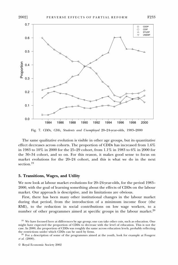
The same qualitative evolution is visible in other age groups, but its quantitativeeffect decreases across cohorts. The proportion of CDDs has increased from 1.6%in 1983 to 10% in 2000 for the 25–29 cohort, from 1.1% in 1983 to 6% in 2000 forthe 30–34 cohort, and so on. For this reason, it makes good sense to focus onmarket evolutions for the 20–24 cohort, and this is what we do in the nextsection.19

5. Transitions, Wages, and Utility

We now look at labour market evolutions for 20–24-year-olds, for the period 1983–2000, with the goal of learning something about the effects of CDDs on the labourmarket. Our approach is descriptive, and its limitations are obvious.

First, there has been many other institutional changes in the labour marketduring that period, from the introduction of a minimum income floor (theRMI), to the reduction in social contributions on low wage workers, to anumber of other programmes aimed at specific groups in the labour market.20

Pro

port

ion

1984 1986 1988 1990 1992 1994 1996 1998 20000.0

0.1

0.2

0.3

0.4

0.5

0.6

0.7CDDPCDIPSTUDPUNEMP

Fig. 7. CDDs, CDIs, Students and Unemployed 20–24-year-olds, 1983–2000

19 We have focused here at differences by age group; one can take other cuts, such as education. Onemight have expected the proportion of CDDs to decrease with the level of education. This is not thecase. In 2000, the proportion of CDDs was roughly the same across education levels, probably reflectingthe restrictions under which CDDs can be used by firms.

20 For a description of some of the programmes aimed at the youth, look for example at Fougereet al. (2000).



We believe, however, that, for the group we focus on below – the 20–24 agegroup – the increase in the proportion of CDDs is indeed the dominantdevelopment.

Second, much of the evolution of unemployment during the period, either forthe 20–24-year-olds or for the population at large, has been due not so much toinstitutional changes but to macroeconomic factors. Until recently, this wouldhave raised a very serious identification issue: from the early 1980s to the late1990s, macroeconomic factors had led to a trend increase in unemployment,making it very difficult to disentangle the effects of that trend from those of thetrend increase in CDDs. Fortunately (both for France and for us), unemploymenthas started decreasing, so there is now hope of disentangling the two. To see whyand how, we start this section by looking at aggregate evolutions.

5.1. Aggregate Evolutions

The top panel of Fig. 8 plots the evolution of the aggregate unemployment rate inFrance since 1983.21 The general picture is of a trend increase from 1983 to themid-1990s, and of a limited decrease since then.

What is relevant to a worker in the labour market is not however the unem-ployment rate per se, but the probabilities of becoming unemployed if he is cur-rently employed, or of becoming employed if he is currently unemployed. Theevolutions of these two transition probabilities are given in the two bottom panelsof Fig. 8. For each panel, the series with squares gives panel transitions, the serieswith triangles gives retrospective transitions.22 We draw two main conclusions fromthese two panels:

� The 1980s appear different from the 1990s. In the 1980s, the transitionprobability from employment to unemployment barely increased, and thetransition probability from unemployment to employment actually increased.By contrast, in the 1990s, the first transition increased, and the seconddecreased: the labour market clearly became worse in both dimensions. Thisworsening surely had a strong effect on the labour market for the 20–24-year-olds we focus on below.

� The panel transition from employment to unemployment was lower in 2000than in any previous year in the sample. The panel transition fromunemployment to employment in 2000 was one of the highest in the sample.

21 For our purposes, the relevant series (in the sense of a series consistent with the other series welook at below) is that from Enquetes Emploi. That series gives a more pessimistic assessment of theevolution of the labour market in France than the series for the official rate. In 2000, the series impliesan unemployment rate of 11.7%, compared to an official rate of 9.7%.

22 We discussed earlier why 1990 is missing for panel transitions, and why 1999 is missing forretrospective transitions. Note that 1995 is also missing for panel transitions in Fig. 8: the reason is thattransitions computed from Enquetes Emploi are very different from those in other years. Most of this isdue to a programme introduced in that year which subsidised the re-employment of the older long-termunemployed, leading to a very different pattern of flows in 1995. Part of it appears to be due to otherproblems with the data. We decided to exclude this year here and in most of the graphs below.



Unemployment rate Trans. prob, E�U Trans. prob, U�E

(a)

(b)

(c)

1983

1984

1985

1986

1987

1988

1989

1990

1991

1992

1993

1994

1995

1996

1997

1998

1999

2000

0.07

0.08

0.09

0.10

0.11

0.12

0.13

0.14

1983

1984

1985

1986

1987

1988

1989

1990

1991

1992

1993

1994

1995

1996

1997

1998

1999

2000

0.02

0

0.02

5

0.03

0

0.03

5

0.04

0

0.04

5

0.05

0

0.05

5

1983

1984

1985

1986

1987

1988

1989

1990

1991

1992

1993

1994

1995

1996

1997

1998

1999

2000

0.28

8

0.30

4

0.32

0

0.33

6

0.35

2

0.36

8

0.38

4

0.40

0

0.41

6

Fig

.8.

Agg

rega

teL

abou

rM

arke

tC

ondi

tion

s,19

83–2

000:

(a)

un

emp

loym

ent

rate

;(b

)tr

ansi

tio

np

rob

abil

ity

fro

mE

toU

;(c

)tr

ansi

tio

np

rob

abil

ity

fro

mU

toE



In other words, despite the fact that the unemployment rate was still high,labour market prospects were, from the point of view of an individual in thelabour market, arguably the best since 1984. Thus a comparison of endpoints– 1984 with 2000 – can help us to separate out the role of cyclical andstructural components. We shall use this below.

5.2. Transition Probabilities for the 20–24-year-olds

Fig. 9 gives the evolution of transition probabilities between CDD employment,CDI employment, and unemployment, for 20–24-year-olds, from 1984 to 1998.Each of the nine panels plots two series. The first, in black, give panel transitions;the second in grey gives retrospective transitions. Transitions for year t refer to thechange in status from March of year t � 1 to March of year t.

We draw three main conclusions from this figure:

� The three left panels show the transition probabilities from unemployment.23

The probability of a CDI decreases in both subperiods (the 1980s and the1990s). The probability of a CDD increases in both subperiods. Bothmovements are clearly consistent with the theory.

While the effect is theoretically ambiguous, we saw that the duration ofunemployment was likely to decrease as the scope of CDDs increased. Theprobability of remaining unemployed indeed decreases in the 1980s.However, there is no evidence of a further decrease in the 1990s. (Notethat the retrospective measure is much higher than the panel measure, butshows the same evolution.) In other words, during the 1990s, the higherlikelihood of a CDD rather than a CDI did not come with an overallincrease in the probability of obtaining a job.

� The three centre panels show the transition probabilities from CDDemployment.

The probability of moving from a CDD to a CDI decreases in each of the twosubperiods. The probability of remaining on a CDD (the same or anotherone) increases throughout the period, nearly doubling in each of the twosubperiods (Recall that the level shifts between 1989 to 1991, which are oftenlarge in the figure, reflect largely differences in measurement.) Note, again,that while panel and retrospective transitions have rather different levels, theirevolution is largely similar over time. The probability of becoming unem-ployed decreases steadily in the 1980s. As we look at year-to-year transitions,this presumably reflects the higher probability of finding another job whenthe current CDD comes to an end. Again, through, there appears to be adifference across the two decades. In the 1990s, the transition probability doesnot exhibit much of a trend.

23 The transition probabilities sum to less than one, as we do not report transitions to selfemployment, internships, military status, student status and other non participation.



1984

1986

1988

1990

1992

1994

1996

1998

2000

0.12

0.14

0.16

0.18

0.20

0.22

0.24

0.26

0.28

1984

1986

1988

1990

1992

1994

1996

1998

2000

0.05

0

0.07

5

0.10

0

0.12

5

0.15

0

0.17

5

0.20

0

0.22

5

0.25

0

1984

1986

1988

1990

1992

1994

1996

1998

2000

0.37

5

0.40

0

0.42

5

0.45

0

0.47

5

0.50

0

0.52

5

0.55

0

0.57

5

1984

1986

1988

1990

1992

1994

1996

1998

2000

0.10

0.15

0.20

0.25

0.30

0.35

0.40

0.45

0.50

0.55

1984

1986

1988

1990

1992

1994

1996

1998

2000

0.15

0.20

0.25

0.30

0.35

0.40

0.45

0.50

0.55

0.60

1984

1986

1988

1990

1992

1994

1996

1998

2000

0.10

0

0.12

5

0.15

0

0.17

5

0.20

0

0.22

5

0.25

0

0.27

5

CD

I to

CD

I

CD

I to

CD

D

CD

I to

U

CD

D to

CD

I

CD

D to

CD

D

CD

D to

U

U to

CD

I

U to

CD

D

U to

U

1984

1986

1988

1990

1992

1994

1996

1998

2000

0.79

0.80

0.81

0.82

0.83

0.84

0.85

0.86

0.87

0.88

1984

1986

1988

1990

1992

1994

1996

1998

2000

0.01

0.02

0.03

0.04

0.05

0.06

0.07

0.08

1984

1986

1988

1990

1992

1994

1996

1998

2000

0.04

5

0.05

0

0.05

5

0.06

0

0.06

5

0.07

0

0.07

5

0.08

0

0.08

5

Fig

.9.

Tra

nsi

tion

Pro

babi

liti

es.

U,

CD

I,C

DD

20–2

4-ye

ar-o

lds,

1984

–200

0



� The three right panels of Fig. 9 show transition probabilities fromCDI employment. They are less central to our discussion (indeed inour formal model, these three transition probabilities were all equal tozero, by assumption). One evolution is, however, worth mentioning. Onemight have expected that allowing firms to use CDDs would have reducedthe flows from CDI employment. The top panel show that this has notbeen the case: the probability of keeping a CDI has decreased, notincreased. This suggests that other factors than changes in firing costshave played a role in determining general trends in separations.

To summarise: the transition probabilities give a picture of a labour market for20–24-year-olds where the probability of a CDD has steadily increased, the prob-ability of a CDI has decreased, and the probability of staying or becoming un-employed shows no clear trend. In this last dimension, there appears to be adifference across the two decades. The probabilities of becoming unemployedwhen on a CDD, or remaining unemployed, both decrease in the 1980s, but showno further trend in the 1990s.

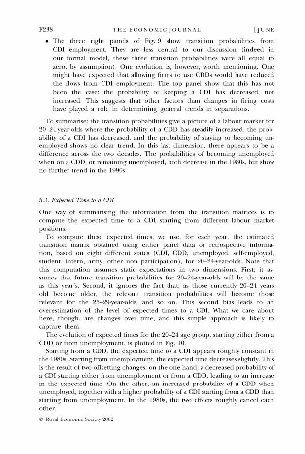
5.3. Expected Time to a CDI

One way of summarising the information from the transition matrices is tocompute the expected time to a CDI starting from different labour marketpositions.

To compute these expected times, we use, for each year, the estimatedtransition matrix obtained using either panel data or retrospective informa-tion, based on eight different states (CDI, CDD, unemployed, self-employed,student, intern, army, other non participation), for 20–24-year-olds. Note thatthis computation assumes static expectations in two dimensions. First, it as-sumes that future transition probabilities for 20–24-year-olds will be the sameas this year’s. Second, it ignores the fact that, as those currently 20–24 yearsold become older, the relevant transition probabilities will become thoserelevant for the 25–29-year-olds, and so on. This second bias leads to anoverestimation of the level of expected times to a CDI. What we care abouthere, though, are changes over time, and this simple approach is likely tocapture them.

The evolution of expected times for the 20–24 age group, starting either from aCDD or from unemployment, is plotted in Fig. 10.

Starting from a CDD, the expected time to a CDI appears roughly constant inthe 1980s. Starting from unemployment, the expected time decreases slightly. Thisis the result of two offsetting changes: on the one hand, a decreased probability ofa CDI starting either from unemployment or from a CDD, leading to an increasein the expected time. On the other, an increased probability of a CDD whenunemployed, together with a higher probability of a CDI starting from a CDD thanstarting from unemployment. In the 1980s, the two effects roughly cancel eachother.



The picture is different in the 1990s, where the expected time increases signi-ficantly until the late 1990s, declining partially thereafter. While the expected timebased on retrospective information is higher than the expected time based onpanel data, both series rise during the period. The expected time from unem-ployment based on retrospective information increases from 4.8 years in 1990 to8.2 years in 1996, to decline to 6.5 years in 2000; its panel data counterpart goesfrom 4.0 to 6.0, down to 4.7 years in 2000.

Num

ber

of y

ears

1983 1985 1987 1989 1991 1993 1995 1997 19992.4

3.2

4.0

4.8

5.6

6.4

7.2

8.0

Num

ber

of y

ears

1983 1985 1987 1989 1991 1993 1995 1997 19993.6

4.2

4.8

5.4

6.0

6.6

7.2

7.8

8.4

(a)

(b)

Fig. 10. Expected Time to a Regular Job: (a) starting from a CDD; (b) starting fromunemployment



5.4. Wages

A complete picture requires looking also at wages. To do so, we run a standardwage regression, regressing for each year, from 1983 to 2000, the logarithm of themonthly net wage on a set of controls – education (15 categories), age (10 cat-egories) and a dummy, D, equal to 1 if the worker is on a CDD, 0 if on a CDI:

log wi ¼ Xib þ bD þ �i

Fig. 11 plots the time series of estimated bs, from estimation of the wage equationfor each year from 1983 to 1998. Given age and education, CDDs appear to payabout 20% less than CDIs. The evidence suggests also that the gap between the twowages has increased over time, from 12% in 1983 to 29% in 1993, and to 22.5% in2000.

5.5. Values

In our model, the welfare effects of partial reform are captured by what happens toV u , the expected present value of utility if currently unemployed. It is tempting toconstruct an empirical counterpart and see how it has evolved over time. This iswhat we do in this last subsection. More specifically, because not all entrants enteras unemployed, we construct not V u , but the average value �VV , the average ex-pected present value of utility for a 20–24-year-old, and look at its evolution overtime.

1984 1986 1988 1990 1992 1994 1996 1998 2000-0.300

-0.275

-0.250

-0.225

-0.200

-0.175

-0.150

-0.125

-0.100

Fig. 11. (Log) Wage Discount for CDDs, with Controls 1983–2000



The results of this exercise must obviously be interpreted with more than a grainof salt: there are many assumptions and many steps involved in the construction of�VV , all likely to imply substantial measurement error. Nevertheless, we think thisprovides a simple way of summarising what we have seen about the evolutions oftransition probabilities and wages in a single statistic.

Let V i be the expected present value of utility conditional on being in state itoday. We consider five states in our computation (CDI, CDD, unemployed, intern,self employed).24 Let V be the associated vector of utilities associated with thedifferent states. Let A be the transition matrix associated with these different states.Let w be the vector of wages or wage equivalents associated with each state. Then,we construct V as

V ¼ w þ 1

1 þ rAV:

Or equivalently,

V ¼ ðI � 1

1 þ rAÞ�1w:

�VV is then constructed as

�VV ¼X

piVi

where the pi are the proportions of individuals in state i, and sum to one, and Vi

are the elements of V.We focus on the 20–24 age group. For A, we use for each year the estimated

transition matrix obtained using either panel data or retrospective information.Just as for the construction of expected times earlier, this computation assumesstatic expectations in two dimensions, ie an unchanged value of the matrix fora given age group over time, and an unchanged transition matrix as individualsin the group grow older. The justification is simplicity, and our belief that, asevolutions are qualitatively similar across age groups, this should capture therelevant trends.

For w, we normalise the CDI wage to 1 (ie we ignore general wage growth overtime). We take the CDD wage to be equal to 1 minus the discount shown in Fig. 11for each year. Based on unemployment benefit rules, we use a value of 0.5 for thewage equivalent when unemployed. Because the transition probabilities to otherstates are small, the other elements of w play little role in the results; we assumea value of 1 for self-employment income, a value equal to the CDD wage forinternships. We use an annual interest rate of 12%.

The results are presented in the top panel of Fig. 12. The black line gives theseries for �VV using panel transitions; the grey line gives the series using retro-spective transitions.

24 Note that we exclude three states: student, army and out of the labour force. If these states wereincluded, our results would be much stronger (ie show a larger decline in �VV .) This is because, if the flowutility of being a student is assumed to be low relative to the wage, the increase in the proportion ofstudents would dominate the series, and lead to a large downward trend in �VV . This trend, however,would be largely unrelated to the issue at hand, namely the role of CDDs.



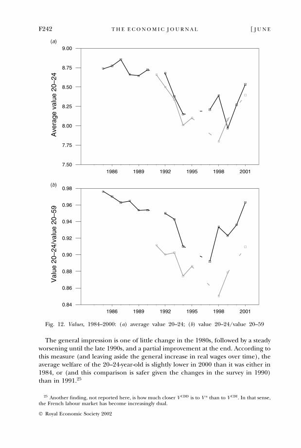
The general impression is one of little change in the 1980s, followed by a steadyworsening until the late 1990s, and a partial improvement at the end. According tothis measure (and leaving aside the general increase in real wages over time), theaverage welfare of the 20–24-year-old is slightly lower in 2000 than it was either in1984, or (and this comparison is safer given the changes in the survey in 1990)than in 1991.25

Ave

rage

val

ue 2

0–24

1986 1989 1992 1995 1998 20017.50

7.75

8.00

8.25

8.50

8.75

9.00V

alue

20–

24/v

alue

20–

59

1986 1989 1992 1995 1998 20010.84

0.86

0.88

0.90

0.92

0.94

0.96

0.98

(a)

(b)

Fig. 12. Values, 1984–2000: (a) average value 20–24; (b) value 20–24/value 20–59

25 Another finding, not reported here, is how much closer V CDD is to V u than to V CDI. In that sense,the French labour market has become increasingly dual.



Can we conclude from this that the effects of CDDs have been perverse? Theanswer is obviously not. Many other factors have been relevant during that period,and attributing all the change in �VV to the introduction of CDDs would obviously bewrong. However, we can make some progress.

Clearly much of the decrease in �VV , especially in the 1990s, must have been dueto macroeconomic factors, rather than to the increase in the proportion of CDDs.Here, the evidence from year 2000 is helpful. As we saw earlier, in terms of ag-gregate transition probabilities, 2000 is arguably the best year of the sample. Yet, inthat year �VV is still lower than it was in either 1984, or 1991. In short, the lower valueof �VV in 2000 cannot easily be attributed to macroeconomic factors.

We can actually go one step further. Some of the changes in �VV are likely toreflect structural changes in the labour market other than CDDs, changes whichmight affect all cohorts. In that case, attributing the decline in �VV over the sampleto the introduction of CDDs would clearly be wrong. This suggests looking not atthe evolution of the average value �VV for the 20–24 age group, but rather at theevolution of this average value relative to the average value for the whole labourforce – which is much less affected by the introduction of CDDs.

With this motivation, we plot the evolution of the ratio of the average value forthe 20–24 age group to the average value for the 20–59 age group in the bottompanel of Fig. 12 (We use the same wages for both groups, thus not taking intoaccount the age profile of wages in computing the two values. This would changethe level, but not the evolution, of the ratio over time.)

The graph has two main characteristics: there is a nearly continuous decline inthe relative value from 1984 to 1997, then an increase, but to a lower level than atthe start of the sample. This suggests two conclusions. First, much of the evolutionof the relative value for the 20–24 age group reflects aggregate evolutions, the longworsening and the recent improvement in the labour market: the young suffermore in a depressed labour market. Second, the fact that the value remains lowerin 2000 suggests that more has been at work. The extension of CDDs, whichdisproportionately affects that group, is a plausible candidate explanation for thisunderlying deterioration. Put more conservatively, there is no evidence that theintroduction and development of CDDs has improved the relative welfare of thosemost affected by it, namely the young.

6. Conclusions

We have looked at the effects of the introduction of fixed-term contracts.On the theoretical side, we argued that the effects of such partial reform

may be perverse, leading to higher turnover and, possibly, lower welfare. Theexcess turnover induced by the forced coexistence of fixed-term and regularcontracts can be high enough to offset the efficiency gains of improvedflexibility.

On the empirical side, we looked at the evolution of labour market experiencesfor young workers in France since 1983. We found strong evidence of increasedturnover, and argued that, if anything, the effect of the fixed-term contracts on thewelfare of young workers appears to have been negative.



If our theoretical and empirical conclusions are valid, this suggests that, at leastfrom an economic viewpoint (ie leaving aside political economy implications),such partial reform may be a very poor substitute for broader reform, i.e. an acrossthe board reduction in firing costs for all workers.

Many questions remain open for future research. To us, the most important maybe how such a reform affects the nature of the jobs offered to workers. We haveassumed in our model that contracts had no impact on the nature of the jobs createdby firms. There are good theoretical and empirical reasons to think they have. Thereare two potential effects at work (which parallel the two effects at work on firms’decisions in our model). On the one hand, lower costs on fixed-term contracts givemore incentives for firms to take more risks, and to design jobs which, associatedwith the right worker, lead to high productivity. On the other, lower costs on fixed-term contracts may instead induce firms to design routine, low productivity jobs,which they can fill through the use of fixed-term contracts. The wage evidence wereviewed in our paper suggests that this second effect might indeed be at work.

References

Adam, P. and Canziani, P. (1998). ‘Partial de-regulation: fixed-term contracts in Italy and Spain’,CEP DP 386.

Blanchard, O. and Portugal, P. (2001). ‘What hides behind an unemployment rate: ComparingPortuguese and U.S. unemployment’, American Economic Review, vol. 91(1), pp. 187–207.

Caballero, R. and Hammour, M. (1996). ‘The ‘‘fundamental transformation’’ in macroeconomics’,American Economic Review, vol. 86(2), pp. 181–6.

Cahuc, P. and Postel-Vinay, F. (2000). ‘Temporary jobs, employment protection, and labor marketperformance’, mimeo, Cepremap, Paris.

Fougere, D., Kramarz, F., and Magnac, T. (2000). ‘Youth employment policies in France’, CEPRDP 2394.

Guell-Rotllan, M. and Petrongolo, B. (2000). ‘Workers’ transitions from temporary to permanentemployment: the Spanish case’, CEP DP 438.

Lamy (2000). Lamy Social, Paris: Editions Lamy.Lazear, E. (1990). ‘Job security provisions and employment’, Quarterly Journal of Economics,

vol. 105(3), pp. 699–726.Magnac, T. and Visser, M. (1999). ‘Transition models with measurement errors’, Review of

Economics and Statistics, vol. 81(3), pp. 466–74.OECD (1999). OECD Employment Outlook, OECD.Philippon, T. (2000). ‘Memory management’, mimeo, MIT.Poulain, G. (1994). Les Contrats de Travail a Duree Determinee, Paris: Litec.Saint-Paul, G. (1996). ‘On the political economy of labor market flexibility’, NBER Macroeconomics

Annual, vol. 8, pp. 151–96.Saint-Paul, G. (2000). The Political Economy of Labor Market Reforms, Oxford: Oxford University Press,

forthcoming.Shapiro, C. and Stiglitz, J. (1984). ‘Equilibrium unemployment as a discipline device’, American

Economic Review, vol. 74, pp. 433–44.

F244 [ J U N E 2002]T H E E C O N O M I C J O U R N A L


Documents

THE PERVERSE EFFECTS OF PARTIAL LABOUR … · THE PERVERSE EFFECTS OF PARTIAL LABOUR MARKET REFORM: FIXED-TERM CONTRACTS ... The main effect may be high turnover in ... productivity