The Plaid Model

by

Richard Evan Schwartz

1

Contents

0.1 Part 1: The Plaid Model . . . . . . . . . . . . . . . . . . . . . 140.2 Part 2: The Plaid Master Picture Theorem . . . . . . . . . . . 150.3 Part 3: The Arithmetic Graph . . . . . . . . . . . . . . . . . . 160.4 Part 4: The Quasi Isomorphism Theorem . . . . . . . . . . . . 160.5 Part 5: The Distribution of Orbits . . . . . . . . . . . . . . . . 180.6 Companion Program . . . . . . . . . . . . . . . . . . . . . . . 20

I The Plaid Model 21

1 Two Definitions of the Plaid Model 221.1 Basic Parameters . . . . . . . . . . . . . . . . . . . . . . . . . 221.2 Six Families of Lines . . . . . . . . . . . . . . . . . . . . . . . 221.3 Capacity, Mass, and Sign . . . . . . . . . . . . . . . . . . . . . 241.4 First Definition of the Plaid Model . . . . . . . . . . . . . . . 251.5 Second Definition of the Plaid Model . . . . . . . . . . . . . . 281.6 The Directed Version . . . . . . . . . . . . . . . . . . . . . . . 30

2 Basic Properties of the Model 322.1 A Characterization of the Masses and Capacities . . . . . . . . 322.2 Symmetries . . . . . . . . . . . . . . . . . . . . . . . . . . . . 332.3 Symmetry and Direction . . . . . . . . . . . . . . . . . . . . . 352.4 The Number of Intersection Points . . . . . . . . . . . . . . . 362.5 Capacity and Mass . . . . . . . . . . . . . . . . . . . . . . . . 37

3 Using the Model 393.1 The Big Polygon . . . . . . . . . . . . . . . . . . . . . . . . . 393.2 Hierarchical Information . . . . . . . . . . . . . . . . . . . . . 413.3 Subdivision Algorithm . . . . . . . . . . . . . . . . . . . . . . 453.4 Grid Lines as Barriers . . . . . . . . . . . . . . . . . . . . . . 47

4 Three Dimensional Construction 504.1 Remote Adjacency . . . . . . . . . . . . . . . . . . . . . . . . 504.2 Horizontal Particles . . . . . . . . . . . . . . . . . . . . . . . . 514.3 Vertical Particles . . . . . . . . . . . . . . . . . . . . . . . . . 534.4 Stacking the Blocks . . . . . . . . . . . . . . . . . . . . . . . . 554.5 Pixellated Spacetime Diagrams . . . . . . . . . . . . . . . . . 57

2

4.6 Spacetime Plaid Surfaces . . . . . . . . . . . . . . . . . . . . . 594.7 The Simplest Example . . . . . . . . . . . . . . . . . . . . . . 614.8 A Remark about Rescaling Limits . . . . . . . . . . . . . . . . 62

5 Directed Spacetime Diagrams 635.1 The Basic Definition . . . . . . . . . . . . . . . . . . . . . . . 635.2 The Curve Turning Process . . . . . . . . . . . . . . . . . . . 645.3 Two Exclusion Principles . . . . . . . . . . . . . . . . . . . . . 655.4 Proof of the Curve Turning Theorem . . . . . . . . . . . . . . 66

6 Connection to the Truchet Tile System 706.1 Truchet Tilings . . . . . . . . . . . . . . . . . . . . . . . . . . 706.2 The Truchet Comparison Theorem . . . . . . . . . . . . . . . 726.3 A Result from Elementary Number Theory . . . . . . . . . . . 756.4 Proof of the Truchet Comparison Theorem . . . . . . . . . . . 776.5 Symmetry of the Horizontal Diagrams . . . . . . . . . . . . . 806.6 Symmetry of the Vertical Diagrams . . . . . . . . . . . . . . . 81

II The Plaid Master Picture Theorem 83

7 The Plaid Master Picture Theorem 847.1 The Spaces . . . . . . . . . . . . . . . . . . . . . . . . . . . . 847.2 The Partition . . . . . . . . . . . . . . . . . . . . . . . . . . . 857.3 The Map . . . . . . . . . . . . . . . . . . . . . . . . . . . . . . 897.4 Three Dimensional Interpretation . . . . . . . . . . . . . . . . 917.5 The Main Result . . . . . . . . . . . . . . . . . . . . . . . . . 927.6 The Undirected Result . . . . . . . . . . . . . . . . . . . . . . 93

8 The Images of Particles 948.1 Overview . . . . . . . . . . . . . . . . . . . . . . . . . . . . . . 948.2 The Vertical Case . . . . . . . . . . . . . . . . . . . . . . . . . 958.3 The Horizontal P Case . . . . . . . . . . . . . . . . . . . . . . 958.4 The Horizontal Q Case . . . . . . . . . . . . . . . . . . . . . . 96

9 Proof of the Main Result 989.1 Symmetric Instances . . . . . . . . . . . . . . . . . . . . . . . 989.2 Sharp Containers . . . . . . . . . . . . . . . . . . . . . . . . . 999.3 Prism Structure . . . . . . . . . . . . . . . . . . . . . . . . . . 101

3

9.4 The Vertical Case . . . . . . . . . . . . . . . . . . . . . . . . . 1039.5 The Horizontal Case . . . . . . . . . . . . . . . . . . . . . . . 105

10 Proof of the Vertical Lemma 10710.1 Outline . . . . . . . . . . . . . . . . . . . . . . . . . . . . . . . 10710.2 Using Symmetry . . . . . . . . . . . . . . . . . . . . . . . . . 10710.3 Translating the Picture . . . . . . . . . . . . . . . . . . . . . . 10810.4 Forgetting the Directions . . . . . . . . . . . . . . . . . . . . . 10910.5 Some Useful Formulas . . . . . . . . . . . . . . . . . . . . . . 11010.6 The Undirected Result . . . . . . . . . . . . . . . . . . . . . . 11110.7 Determining the Directions . . . . . . . . . . . . . . . . . . . . 113

11 Proof of The Horizontal Lemma 11411.1 Using Symmetry . . . . . . . . . . . . . . . . . . . . . . . . . 11411.2 Translating the Picture . . . . . . . . . . . . . . . . . . . . . . 11511.3 A Technical Lemma . . . . . . . . . . . . . . . . . . . . . . . . 11611.4 The Undirected Result . . . . . . . . . . . . . . . . . . . . . . 11611.5 Determining the Directions . . . . . . . . . . . . . . . . . . . . 117

III The Graph Master Picture Theorem 119

12 The Arithmetic Graph 12012.1 Special Orbits and the First Return Map . . . . . . . . . . . . 12012.2 The Arithmetic Graph . . . . . . . . . . . . . . . . . . . . . . 12112.3 The Canonical Affine Transformation . . . . . . . . . . . . . . 12312.4 Geometry of the Graph Grid . . . . . . . . . . . . . . . . . . . 124

13 Graph Master Picture Theorem 12913.1 Statement of the Result . . . . . . . . . . . . . . . . . . . . . 12913.2 Pulling Back the Maps . . . . . . . . . . . . . . . . . . . . . . 13113.3 Further Discussion . . . . . . . . . . . . . . . . . . . . . . . . 13113.4 The Fundamental Polytopes . . . . . . . . . . . . . . . . . . . 133

14 Pinwheels and Quarter Turn Systems 13514.1 Overview . . . . . . . . . . . . . . . . . . . . . . . . . . . . . . 13514.2 The Pinwheel Map . . . . . . . . . . . . . . . . . . . . . . . . 13614.3 Outer Billiards and the Pinwheel Map . . . . . . . . . . . . . 13814.4 Quarter Turn Compositions . . . . . . . . . . . . . . . . . . . 139

4

14.5 The Pinwheel Map as a QTS . . . . . . . . . . . . . . . . . . . 14014.6 The Case of Kites . . . . . . . . . . . . . . . . . . . . . . . . . 143

15 The General Compactification 14515.1 Affine Pets Redefined . . . . . . . . . . . . . . . . . . . . . . . 14515.2 The Map . . . . . . . . . . . . . . . . . . . . . . . . . . . . . . 14615.3 Extending The Component Maps . . . . . . . . . . . . . . . . 14715.4 The Composition . . . . . . . . . . . . . . . . . . . . . . . . . 14915.5 Double Lattice PETs . . . . . . . . . . . . . . . . . . . . . . . 15015.6 The Structure Theorem . . . . . . . . . . . . . . . . . . . . . . 15115.7 The General Arithmetic Graph . . . . . . . . . . . . . . . . . 15215.8 The Case of Kites . . . . . . . . . . . . . . . . . . . . . . . . . 153

16 Proof of the Structure Theorem 15516.1 The Singular Directions . . . . . . . . . . . . . . . . . . . . . 15516.2 The First Parallelotope . . . . . . . . . . . . . . . . . . . . . . 15716.3 The Second Parallelotope . . . . . . . . . . . . . . . . . . . . 15916.4 The Fixed Point Set . . . . . . . . . . . . . . . . . . . . . . . 160

IV The Quasi-Isomorphism Theorem 162

17 The Proof in Broad Strokes 16317.1 Pixellated Squares . . . . . . . . . . . . . . . . . . . . . . . . 16317.2 Bad Squares . . . . . . . . . . . . . . . . . . . . . . . . . . . . 16417.3 Errand Edges and Double Crossings . . . . . . . . . . . . . . . 16617.4 The Pixellation Theorem . . . . . . . . . . . . . . . . . . . . . 16717.5 The Bound Chain Lemma . . . . . . . . . . . . . . . . . . . . 16817.6 Proof of the Quasi-Isomorphism Theorem . . . . . . . . . . . . 169

18 Proof of the Bound Chain Lemma 17218.1 Length Two Chains . . . . . . . . . . . . . . . . . . . . . . . . 17218.2 Length Three Chains: Case A . . . . . . . . . . . . . . . . . . 17318.3 Length Three Chains: Case B . . . . . . . . . . . . . . . . . . 17518.4 Length Three Chains: Case C . . . . . . . . . . . . . . . . . . 17618.5 Length Four Chains: Case A . . . . . . . . . . . . . . . . . . . 18118.6 Length Four Chains: Case B . . . . . . . . . . . . . . . . . . . 18218.7 Length Four Chains: Case C . . . . . . . . . . . . . . . . . . . 183

5

18.8 Length Four Chains: Case D . . . . . . . . . . . . . . . . . . . 184

19 The Graph Reconstruction Formula 18619.1 Main Result . . . . . . . . . . . . . . . . . . . . . . . . . . . . 18619.2 Eliminating Most Double Crossings . . . . . . . . . . . . . . . 18819.3 Eliminating the last Double Crossing . . . . . . . . . . . . . . 189

20 The Hitset and the Intertwiner 19120.1 The Hitset . . . . . . . . . . . . . . . . . . . . . . . . . . . . . 19120.2 The Projective Intertwiner . . . . . . . . . . . . . . . . . . . . 19320.3 Well Definedness . . . . . . . . . . . . . . . . . . . . . . . . . 19520.4 Strategy of the Proof . . . . . . . . . . . . . . . . . . . . . . . 19620.5 The Intertwining Theorem on the Diagonal . . . . . . . . . . . 19720.6 The Hitset Theorem on the Diagonal . . . . . . . . . . . . . . 19920.7 Hitset Induction . . . . . . . . . . . . . . . . . . . . . . . . . . 20020.8 Changing the Fundamental Domain . . . . . . . . . . . . . . . 20220.9 Intertwiner Induction . . . . . . . . . . . . . . . . . . . . . . . 20420.10Proof of the Geometric Claim . . . . . . . . . . . . . . . . . . 205

21 Correspondence of Polytopes 20721.1 The Triple Partition . . . . . . . . . . . . . . . . . . . . . . . 20721.2 Proof of Statement 2 . . . . . . . . . . . . . . . . . . . . . . . 20921.3 A Sample Result . . . . . . . . . . . . . . . . . . . . . . . . . 21021.4 Fixing Orientations . . . . . . . . . . . . . . . . . . . . . . . . 21221.5 Edge Crossing Problems . . . . . . . . . . . . . . . . . . . . . 214

22 Edge Crossings 21622.1 The Graph Method . . . . . . . . . . . . . . . . . . . . . . . . 21622.2 The Sample Result Revisited . . . . . . . . . . . . . . . . . . . 21822.3 The Plaid Method . . . . . . . . . . . . . . . . . . . . . . . . 220

22.3.1 Case 1 . . . . . . . . . . . . . . . . . . . . . . . . . . . 22122.3.2 Case 2 . . . . . . . . . . . . . . . . . . . . . . . . . . . 22122.3.3 Case 3 . . . . . . . . . . . . . . . . . . . . . . . . . . . 22222.3.4 Case 4 . . . . . . . . . . . . . . . . . . . . . . . . . . . 22222.3.5 Case 5 . . . . . . . . . . . . . . . . . . . . . . . . . . . 222

22.4 Another Edge Crossing Problem . . . . . . . . . . . . . . . . . 22322.5 Out of Bounds . . . . . . . . . . . . . . . . . . . . . . . . . . 223

6

23 Proof of the Pixellation Theorem 22523.1 Solving Most of the Crossing Problems . . . . . . . . . . . . . 22523.2 Proof of Statement 3 . . . . . . . . . . . . . . . . . . . . . . . 22523.3 Proof of Statement 4 . . . . . . . . . . . . . . . . . . . . . . . 22623.4 Proof of Statement 5 . . . . . . . . . . . . . . . . . . . . . . . 228

23.4.1 Case 1 . . . . . . . . . . . . . . . . . . . . . . . . . . . 23023.4.2 Case 2 . . . . . . . . . . . . . . . . . . . . . . . . . . . 23123.4.3 Case 3 . . . . . . . . . . . . . . . . . . . . . . . . . . . 23123.4.4 Case 4 . . . . . . . . . . . . . . . . . . . . . . . . . . . 232

24 Computer Assisted Techniques 23324.1 Operations on Polytopes . . . . . . . . . . . . . . . . . . . . . 23324.2 The Calculations . . . . . . . . . . . . . . . . . . . . . . . . . 23524.3 The Computer Program . . . . . . . . . . . . . . . . . . . . . 238

24.3.1 Downloading the Program . . . . . . . . . . . . . . . . 23824.3.2 Running and Compiling . . . . . . . . . . . . . . . . . 23824.3.3 What to do first . . . . . . . . . . . . . . . . . . . . . . 23824.3.4 Presets . . . . . . . . . . . . . . . . . . . . . . . . . . . 23924.3.5 Surveying the Data and Proofs . . . . . . . . . . . . . 239

V The Distribution of Orbits 240

25 Unbounded Orbits 24125.1 Geometric Limits . . . . . . . . . . . . . . . . . . . . . . . . . 24125.2 Approximating Irrationals . . . . . . . . . . . . . . . . . . . . 24225.3 Arc Copying . . . . . . . . . . . . . . . . . . . . . . . . . . . . 24425.4 The Images of the Anchors . . . . . . . . . . . . . . . . . . . . 24625.5 The End of the Proof . . . . . . . . . . . . . . . . . . . . . . . 248

26 Some Elementary Number Theory 25026.1 All About Predecessors . . . . . . . . . . . . . . . . . . . . . . 250

26.1.1 Statement 1 . . . . . . . . . . . . . . . . . . . . . . . . 25126.1.2 Statement 2 . . . . . . . . . . . . . . . . . . . . . . . . 25126.1.3 Statements 3 and 5 . . . . . . . . . . . . . . . . . . . . 25226.1.4 Statement 4 . . . . . . . . . . . . . . . . . . . . . . . . 25226.1.5 Statement 6 . . . . . . . . . . . . . . . . . . . . . . . . 25326.1.6 Statement 7 . . . . . . . . . . . . . . . . . . . . . . . . 253

7

26.2 Existence of the Predecessor Sequence . . . . . . . . . . . . . 25326.3 Existence of the Approximating Sequence . . . . . . . . . . . . 25426.4 Another Identity . . . . . . . . . . . . . . . . . . . . . . . . . 256

27 The Box Lemma and The Copy Theorem 25827.1 The Weak and Strong Copying Lemmas . . . . . . . . . . . . 25827.2 The Core Copy Lemma . . . . . . . . . . . . . . . . . . . . . . 25927.3 Proof of the Box Lemma . . . . . . . . . . . . . . . . . . . . . 25927.4 Setup for the Copying Theorem . . . . . . . . . . . . . . . . . 26127.5 The Strong Case . . . . . . . . . . . . . . . . . . . . . . . . . 26127.6 The Core Case . . . . . . . . . . . . . . . . . . . . . . . . . . 262

28 The Weak and Strong Copy Lemmas 26428.1 The Mass and Capacity Sequences . . . . . . . . . . . . . . . 26428.2 A Matching Criterion . . . . . . . . . . . . . . . . . . . . . . . 26528.3 Geometric Alignment . . . . . . . . . . . . . . . . . . . . . . . 26728.4 Alignment of the Capacity Sequences . . . . . . . . . . . . . . 26828.5 Alignment of the Mass Sequences . . . . . . . . . . . . . . . . 269

29 The Core Copy Lemma 27229.1 The Difficulty . . . . . . . . . . . . . . . . . . . . . . . . . . . 27229.2 Weak Horizontal Alignment . . . . . . . . . . . . . . . . . . . 27229.3 Geometric Alignment . . . . . . . . . . . . . . . . . . . . . . . 27329.4 Alignment of the Capacity Sequences . . . . . . . . . . . . . . 27329.5 Calculating some of the Masses . . . . . . . . . . . . . . . . . 27629.6 Alignment the Mass Sequences . . . . . . . . . . . . . . . . . . 279

30 Existence of Many Large Orbits 28230.1 The Empty Rectangle Lemma . . . . . . . . . . . . . . . . . . 28230.2 The Ubiquity Lemma . . . . . . . . . . . . . . . . . . . . . . . 28330.3 Proof of the Main Result . . . . . . . . . . . . . . . . . . . . . 28430.4 The Continued Fraction Length . . . . . . . . . . . . . . . . . 28530.5 Circle Rotations . . . . . . . . . . . . . . . . . . . . . . . . . . 28630.6 Proof of the Grid Supply Lemma . . . . . . . . . . . . . . . . 287

31 Tuned Sequences 28831.1 Rescaling the Model . . . . . . . . . . . . . . . . . . . . . . . 28831.2 The Filling Property . . . . . . . . . . . . . . . . . . . . . . . 289

8

31.3 Proof of Theorem 31.1 . . . . . . . . . . . . . . . . . . . . . . 291

32 References 293

9

Preface

The purpose of this monograph is to study a construction, based on elemen-tary geometry and number theory, which produces for each rational parame-ter (satisfying some parity conditions) a cube filled with polyhedral surfaces.When the surfaces are sliced in one direction, the resulting curves turn outto encode all the essential information about outer billiards on kites. Whenthe surfaces are sliced in two other directions, they encode all the essentialinformation in a 1-parameter family of the Truchet tile systems defined in[H]. I call the construction the plaid model.

The plaid model grew out of my work in [S1], where I gave an affirmativeanswer to the Moser-Neumann question about outer billiards: Does thereexist an outer billiards system with an unbounded orbit? The main result of[S1] is that outer billiards has unbounded orbits relative to any irrational kite– a bilaterally symmetric convex quadrilateral which is not affinely equivalentto a lattice polygon.

The plaid model has a physical feel, with properties that seem like conser-vation laws, interacting particles, spacetime diagrams, and even an exclusionprinciple. It also has an overtly hierarchical structure, which causes it toexhibit properties such as self-similarity and scaling limits. Finally, it has aninterpretation in terms of a beautiful higher dimensional polytope exchangetransformation.

This monograph establishes some of the basic properties of the plaidmodel: the connection to outer billiards and to Truchet tilings, the connec-tion to polytope exchange transformations, and some results about the sizeand distribution of the polygons in the slices of the model. I feel that theplaid model is a deep and surprising structure which blends geometry, com-binatorics, number theory, and dynamics. I hope that this work points outits depth and beauty, and suggests topics for further study.

I would like to thank the National Science Foundation for their continuedsupport, and also the Simons Foundation for an upcoming Simons SabbaticalFellowship. I’d also like to thank Peter Doyle, Pat Hooper, Sergei Tabach-nikov, and Ren Yi for a number of conversations related to the plaid model.

10

Introduction

Imagine starting with a square grid, as shown in Figure 0.1. One can produceinteresting patterns of points on the square grid by taking some slanting linesand marking the points where they intersect the grid. The left side of Figure0.1 shows this.

2

0

3

Figure 0.1: Slanting lines intersecting a grid

We could add variety to the construction by assigning “capacities” to thegrid lines and “masses” to the slanting lines, and then putting intersectionpoints only when the mass of the slanting line is less than the capacity ofthe grid line. The right side shows the same example as the left, but withmasses and capacities added.

The plaid model starts out with a construction like this, and then we buildtilings of the plane based on the arrangement of the intersection points. Thetilings in turn define families of embedded polygons. Finally, we cut outvarious chunks (or blocks) of the planar tiling, stack them on top of eachother, and canonically interpolate between the polygons at different levels toform embedded polyhedral surfaces.

The plaid model grew out of a theorem I proved in [S1] which I calledthe Hexagrid Theorem. The Hexagrid Theorem is one of the main structuraltools I used to understand some properties of outer billiards on kites – enoughto prove the following result.

Theorem 0.1 Outer billiards on any irrational kite has an unbounded orbit.

11

Theorem 0.1 resolved the so-called Moser-Neumann problem, from 1960,which asked whether an outer billiards system could ever have an unboundedorbit.

Any kite is affinely equivalent to the kite KA with vertices

(−1, 0), (0, 1), (0,−1), (A, 0). (1)

See Figure 0.2. The kite is (ir)rational when A is (ir)rational. Figure 0.2shows outer billiards on KA for A = 4/9. Given p0 ∈ R2 − A, we define amap p0 → p1 by the rule that the line segment p0p1 is tangent to K at itsmidpoint, and K is on the right hand side as one walks along the segmentfrom p0 to p1. One then considers the orbit p0 → p1 → p2.... See [S1] for anextensive discussion of outer billiards and a long bibliography.

K

p

pp

0

21

p3

Figure 0.2: Outer billiards on the kite K.

We call an outer billiards orbit on KA special if it lies in the union

Ξ = ±1,±3,±5, ... ×R. (2)

Each special orbit returns infinitely often to the pair horizontal rays shownin Figure 0.2. We denote these rays by the symbol =⇒.

The key step in understanding the special orbits on KA is to associate afamily of embedded lattice polygons to the orbits which encodes the symbolicdynamics of the first return map to =⇒. I call these polygonal curves thearithmetic graph. Part 3 of the monograph has a detailed description. In [S1]The Hexagrid Theorem, mentioned above, predicts the large scale structureof the arithmetic graph based on where certain grids of lines intersect.

12

Some years later I discovered that the Hexagrid Theorem was just thefirst in a series of results which allowed this large scale structure to extenddown to increasingly fine scales. When all these results are assembled intoone package, the result is the plaid model. For each parameter A = p/q withpq even, the plaid model construction produces a cubical array of (p + q)3

unit cubes that is filled with disjoint embedded polyhedral surfaces. Whenthese surfaces are sliced in the XY directions they produce curves whichagree with the arithmetic graph associated to KA up to one unit of error.

Figure 0.3: Two XY plaid model slices for the parameter 4/9.

Figure 0.3 shows two consecutive slices of the surfaces for the parameter4/9. Here is a more concrete (though less powerful) way to explain theconnection to outer billiards. When the polygons in Figure 0.3 are projectedonto the X coordinate, each one of them agrees with the first return map ofsome special orbit to =⇒ up to a uniformly bounded error. The bound isabout 4 units, and it works for all parameters.

When the surfaces in the plaid model are sliced in the other directions,namely the XZ and Y Z directions, what emerges (at least for some slices) isa combinatorial pattern of curves that is combinatorially isomorphic to thecurves produced by Pat Hooper’s Truchet tile system [H].

Figure 0.4 gives an example. The plaid model parameter is 4/9 and theTruchet tile parameter is α = β = 3/8.

13

Figure 0.4: A YZ slice for 4/9 compared to a Truchet tiling.

Thus, the 3 dimensional plaid model is a kind of marriage between thesymbolic dynamics of outer billiards on kites and the Truchet tile system.The purpose of this monograph is to explore its structure. The monographhas 5 parts. Here is a detailed description of these parts.

0.1 Part 1: The Plaid Model

In Part 1, I will define the plaid model (in several ways) and study its basicproperties. One thing that is not clear from any of the definitions is that theplaid model is well-defined. There will be several places where the resultsdepend on the consistency of the definitions. I will deduce the claimed con-sistency results at the end of Part 2, as a consequence of the Plaid MasterPicture Theorem.

After studying the basic properties of the model I will explain how one canuse the hierarchical nature to get information about the large scale structureof the tilings in an algorithmic way. In particular, I will give a heuristicexplanation of why the model exhibits coarse self-similarity and rescalingphenomena.

The initial construction of the plaid model produces 2 dimensional slices.I will explain how to assemble these slices into embedded polyhedral surfaces.Finally, I will establish the connection between theXZ and Y Z slices of thesesurfaces and the Truchet tilings. The main theorem along these lines is theTruchet Comparison Theorem from §6.2.

14

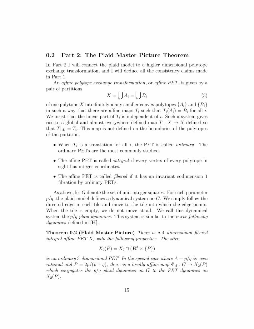
0.2 Part 2: The Plaid Master Picture Theorem

In Part 2 I will connect the plaid model to a higher dimensional polytopeexchange transformation, and I will deduce all the consistency claims madein Part 1.

An affine polytope exchange transformation, or affine PET , is given by apair of partitions

X =⋃

Ai =⋃

Bi (3)

of one polytope X into finitely many smaller convex polytopes Ai and Biin such a way that there are affine maps Ti such that Ti(Ai) = Bi for all i.We insist that the linear part of Ti is independent of i. Such a system givesrise to a global and almost everywhere defined map T : X → X defined sothat T |Ai

= Ti. This map is not defined on the boundaries of the polytopesof the partition.

• When Ti is a translation for all i, the PET is called ordinary . Theordinary PETs are the most commonly studied.

• The affine PET is called integral if every vertex of every polytope insight has integer coordinates.

• The affine PET is called fibered if it has an invariant codimension 1fibration by ordinary PETs.

As above, let G denote the set of unit integer squares. For each parameterp/q, the plaid model defines a dynamical system on G. We simply follow thedirected edge in each tile and move to the tile into which the edge points.When the tile is empty, we do not move at all. We call this dynamicalsystem the p/q plaid dynamics . This system is similar to the curve followingdynamics defined in [H].

Theorem 0.2 (Plaid Master Picture) There is a 4 dimensional fiberedintegral affine PET X2 with the following properties. The slice

X2(P ) = X2 ∩ (R3 × P)

is an ordinary 3-dimensional PET. In the special case where A = p/q is evenrational and P = 2p/(p + q), there is a locally affine map ΦA : G → X2(P )which conjugates the p/q plaid dynamics on G to the PET dynamics onX2(P ).

15

0.3 Part 3: The Arithmetic Graph

As we mentioned above, in [S1] we associate an infinite family of polygonalpaths to each rational parameter A = p/q ∈ (0, 1). These paths are em-bedded and have integer vertices. When pq is even, the paths are all closedembedded polygons. We call these polygons the arithmetic graph.

The significance of the arithmetic graph is that there is a bijection be-tween components of the arithmetic graph and special outer billiards orbits(up to a certain trivial involution on the orbits.) The bijection has the prop-erty that the number of vertices in the component of the arithmetic graphis the same as the number of times the orbit hits the union =⇒ of two raysdefined above. One can recover the outer billiards orbits from the graph.

Just as we have the plaid (curve following) dynamics we have the graph(curve following) dynamics for the arithmetic graph. The graph polygonsare naturally oriented by the outer billiards dynamics, and we simply movefrom each vertex of Z2 to the next. In [S1] we proved the following result,though we stated it somewhat differently.

Theorem 0.3 (Graph Master Picture) Let p/q ∈ (0, 1) be any rationalparameter. There is an ordinary 3 dimensional PET YA and a locally affinemap ΨA : Z2 → YA which conjugates the p/q graph dynamics to the dynamicson YA.

⋃A YA is dense in a 4-dimensional fibered integral affine PET.

In this part of the monograph I will follow my preprint [S3] and putthe Graph Master Picture Theorem in a wider context of higher dimensionalcompactifications which work for an essentially arbitrary polygonal outerbilliards system. This gives a new and more conceptual proof of the GraphMaster Picture Theorem.

0.4 Part 4: The Quasi Isomorphism Theorem

We say that two embedded polygons are C-quasi-isomorphic if they can beparametrized so that corresponding points are within C units of each other.We say that two unions Γ and Π of polygons are C-quasi-isomorphic if thereis a bijection between the members of A and the members of Γ which pairsup C-quasi-isomorphic polygons. Finally, we say that A and B are C-affine-quasi-isomorphic if there is an affine transformation T : R2 → R2 such thatΠ and T (Γ) are C-quasi-isomorphic. Here is the main result.

16

Theorem 0.4 (Quasi-Isomorphism) Let p/q ∈ (0, 1) be any rational suchthat pq is even. Let Π denote the plaid model at the parameter p/q. Let Γdenote the arithmetic graph associated to the special orbits of outer billiardson the kite Kp/q. Then Π and Γ are 2-affine-quasi-isomorphic.

Figure 0.5 shows the Quasi-Isomorphism Theorem in action for the parameterp/q = 4/9. The black polygons are part of the plaid model and the greypolygons are part of a canonically chosen affine image of the arithmetic graph.

Figure 0.5: The Quasi-Isomorphism Theorem in action.

17

In general, the vertices of the black curves lie in the lattice 12Z2, which

has co-area 1/4, whereas the vertices of the grey curves lie in a lattice havingco-area 1 + p/q. Even through the polygons line up in a global sense, theirvertices lie on quite different lattices. This fact points to the highly nontrivialnature of quasi-isomorphism being established.

The Quasi-Isomorphism has a more dynamical formulation.

Theorem 0.5 (Orbit Equivalence) Let X be the affine PET from thePlaid Master Picture Theorem and let Y be the affine PET from the GraphMaster Picture Theorem. There is a fibered polyhedral set Z ⊂ X which in-tersects every orbit on X, and a piecewise integral projective map F : Z → Ywhich carries the fiber ZP to the fiber YA. The map F is an orbit equivalence:It sets up a bijection between the orbits in X and the orbits in Y .

An algebraic set Z is fibered polyhedral if it has a codimension 1 fibrationin which each fiber is a polyhedron. When X is the fibered affine PET fromthe Plaid Master Picture Theorem, we mean for the fibration of X to inducethe fibration of Z.

The Quasi-Isomorphism Theorem is basically a consequence of the PlaidMaster Picture Theorem, the Graph Master Picture Theorem, and the OrbitEquivalence Theorem, but actually the relationship between these theoremsis different. We will first construct the map F : X → Y . Then we will givea computer assisted proof that F has certain combinatorial properties whichimply the Quasi-Isomorphism Theorem. Then we will observe at the endthat we have also proved the Orbit Equivalence Theorem.

0.5 Part 5: The Distribution of Orbits

Part 5 concerns the distribution and geometry of orbits in the plaid model.Say that a set in the plane is fat if it is not contained in a tubular neighbor-hood of any straight line. A fat set, in particular, is unbounded. The PlaidMaster Picture Theorem will allow us to make sense of the plaid model evenat irrational parameters. With this identification, each orbit in the plaidPET corresponds to either a closed plaid polygon or an infinite polygonalpath. The bulk of Part 4 is devoted to proving the following result.

Theorem 0.6 (Unbounded Orbits) For every irrational A ∈ (0, 1) thereexists an infinite orbit in the plaid PET whose corresponding unbounded orbitis a fat path.

18

The idea behind the proof of the Unbounded orbits theorem is to showthat there exist orbits of large diameter in the rational case, and then totake a geometric limit. The geometric limit argument must be done carefullyif we want to end up with an unbounded path that corresponds to a well-defined orbit in the plaid PET. Our analysis will reveal the importance ofDiophantine considerations in the plaid model.

The Quasi-Isomorphism Theorem combines with the Unbounded OrbitsTheorem to give another proof of Theorem 0.1 from [S1].

We define a block to be a single integer horizontal slice of the 3 dimensionalplaid model. Figure 0.3 shows the picture in two different blocks. Our nextresult shows that all the blocks contain long orbits when the parameter iscomplicated.

We say that a plaid polygon isN -fat if it does not lie within theN -tubularneighborhood of any straight line.

Theorem 0.7 Let pk/qk ⊂ (0, 1) be any sequence of even rational numberswith an irrational limit. Let Bk be any sequence of associated blocks. LetN be any fixed integer. Then the number of N -fat plaid polygons in Bk isgreater than N provided that k is sufficiently large.

Theorem 0.8 can be interpreted in terms of outer billiards on the kiteKA when A = p/q. Recall that a special orbit is an orbit which lies on theinvariant set Ξ of horizontal lines having y intercept an odd integer. Everysuch orbit has points in the union =⇒ of two rays that we used for our firstreturn map. Define the essential diameter of a special orbit O to be diameterof O∩ =⇒.

Corollary 0.8 Let pk/qk ⊂ (0, 1) be any sequence of even rational num-bers with an irrational limit. Let Ik be any sequence of intervals of theform [nωk, nωk + ωk]. Let N be any fixed integer. Then there are more thanN distinct orbits in the interval Ik × 1 which have essential diameter atleast N provided that k is sufficiently large.

Corollary 0.8 follows directly from Theorem 0.7 and from the Quasi-Isomorphism Theorem.

When we know more about the sequence of rationals we will be able toget detailed information. Theorem 31.1 is a more specialized result alongthese lines.

19

0.6 Companion Program

The paper comes with a companion computer program which illustrates manyof the results in this paper - in particular the PET Equivalence Theorem.One can download this program from my website. The URL is

http://www.math.brown.edu/∼res/Java/PLAID2.tar

I discovered all the results in this monograph using the program, and I haveextensively checked my proofs against the output of the program. While thismonograph mostly stands on its own, the reader will get much more out ofit by using the program while reading. I would say that the program relatesto the material here the way a cooked meal relates to a recipe.

20

Part I

The Plaid Model

21

1 Two Definitions of the Plaid Model

1.1 Basic Parameters

Throughout the monograph, we work with rational parameters p/q ∈ (0, 1)such that pq is even. We call these parameters even rational parameters .Here are the main auxiliary quantities associated to these parameters.

ω = p+ q, P =2p

ω, Q =

2q

ω. (4)

Note thatP

Q=p

q, P +Q = 2. (5)

We let τ ∈ (0, ω) is the integer such that

2pτ ≡ 1 mod ω. (6)

Finally, we defineτ = min(τ , ω − τ). (7)

So, τ is the unique solution to 2pτ ≡ ±1 mod ω that lies in (0, ω/2).

1.2 Six Families of Lines

We consider 6 infinite families of lines.

• H consists of horizontal lines having integer y-coordinate.

• V consists of vertical lines having integer x-coordinate.

• P± is the set of lines of slope ±P having integer y-intersept.

• Q± is the set of lines of slope ±Q having integer y-intersept.

We call the lines in H and V the grid lines , and we call the other lines theslanting lines . Until the last section of this chapter, we only use the familiesV , H, P− and Q−. We set P = P− and Q = Q− in order to simplify thenotation. Figure 1.1 shows these lines inside [0, 7]2 for p/q = 2/5. In thiscase, P = 4/7 and Q = 10/7.

22

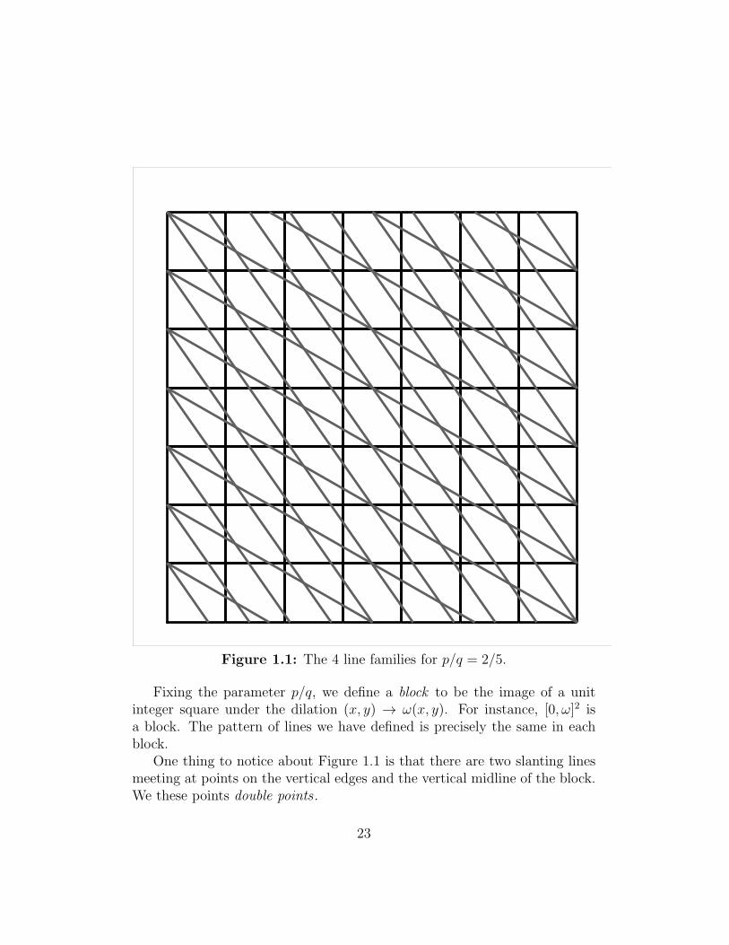
Figure 1.1: The 4 line families for p/q = 2/5.

Fixing the parameter p/q, we define a block to be the image of a unitinteger square under the dilation (x, y) → ω(x, y). For instance, [0, ω]2 isa block. The pattern of lines we have defined is precisely the same in eachblock.

One thing to notice about Figure 1.1 is that there are two slanting linesmeeting at points on the vertical edges and the vertical midline of the block.We these points double points .

23

1.3 Capacity, Mass, and Sign

Given some integer N and some integer a, we define (a)2N to be the repre-sentative of a mod 2N in (−N,N). If a ≡ N mod 2N we define a2N = ∗N ,a symbol which denotes the set N,−N.

We associate signs and capacities to all the lines in H and V as follows.

• The signed capacity of the line y = y0 is (4py0)2ω.

• The signed capacity of the line x = x0 is (4px0)2ω.

• The signed mass if a slanting line through (0, y) is (2py + ω)2ω.

Sometimes we will want to consider the signs or the absolute values ofthe quantities just defined. We define the capacity of a grid line to be theabsolute value of its signed capacity. We define the sign of a grid line to bethe sign of its capacity. Likewise we define the quantities mass and sign forthe slanting lines. When the capacity or mass is 0, the sign is indeterminate.Note that the capacity is never ±ω, so it is always well defined.

Figure 1.2 shows the assignment of these quantities to the lines in thesquare [0, 7]2. The black labels are the signed capacities and the grey labelsare the signed masses.

-2

+2

+4

+6

-4

-6

0

0-6 +2 -4 +4 -2+6 00

*7

-3

+1

+5

-5

-1

+3

*7

Figure 1.2: The mass and capacity labels for p/q = 2/5.

24

1.4 First Definition of the Plaid Model

We say that an intersection point on a grid line is the intersection of thatgrid line with a slanting line. Suppose that γ is a grid line and v ∈ γ is theintersection of γ with a slanting line σ. We call v light (with respect to thesetwo lines) if and only if

• σ and γ have the same sign.

• The mass of σ is less than the capacity of γ.

Otherwise we call v dark . These features of an intersection point will becalled its shade.

We take special care when v lies on a double point.

Midline Case: Suppose that v lies on the vertical midline of a block. Inthis case, v lies on a horizontal grid line but not a vertical grid line. Thetwo slanting lines through v have y-intercepts which are ω apart, so v wouldbe reckoned light with respect to both slanting lines, or dark with respect toboth slanting lines. Accordingly, we count v either as 2 light points or as 2dark points.

Corner Case: The intersection points on the vertical edges of the blockare all grid points. That is, they have integer coordinates. Such points lieon 2 slanting lines. Let v be such a point. The left and right edges of eachblock have capacity 0, so v is considered a dark point on the vertical line. Onthe other hand, if we think of v as being a point on the horizontal line thatcontains it, we count v as a single light point or a single dark point accordingto the definition above, taken with respect to either slanting line containing v.

Figure 1.3 below shows the light intersection points inside the square[0, 7]2 for the parmeter 2/5. For each unit square S in this region, we haveconnected the center of S to the light points on ∂S.

Notice that some interesting curves seem to emerge. Notice also that thereseems to be a small amount of junk, in the form of little loops, hanging offthese curves. The junk occurs wherever there are two light points in a singleedge. The one exception appears to be the case when the edge intersects thevertical midline (right in the center of the picture) but in this case the onelight point on each relevant horizontal edge is counted twice.

25

Figure 1.3: The light points in [0, 7]2 with respect to p/q = 2/5.

We say that a unit integer square is a unit square whose vertices haveinteger coordinates. Such squares are bounded by grid lines. We call theedges of such a square unit segments . Such segments, of course, either lie onH lines or on V lines.

We say that a unit segment is good if it contains exactly one light point.The points are reckoned with respect to the grid containing the edge. Thus,for the boundary cases considered in the previous section, the point might belight with respect to the horizontal edge containing it, but it would alwaysbe dark with respect to the vertical edge containing it.

26

We say that a unit square is coherent if it contains either 0 or 2 goodsegments. We say that the plaid model is coherent at if all squares arecoherent for all parameters. Here is the fundamental theorem concerning theplaid model.

Theorem 1.1 The plaid model is coherent for all parameters.

Theorem 1.1 is an immediate consequence of the Plaid Master Picture The-orem, which we prove in Part 2 of the monograph.

Theorem 1.1 allows us to create a union of embedded polygons. In eachunit square we draw the line segment which connects the center of the squarewith the centers of its good edges. The squares with no good edges simplyremain empty. We call these polygons the plaid polygons . Figure 1.4 showsthe plaid polygons contained in [0, 7]2 for the parameter 2/5. Of course, theseplaid polygons fill the entire plane, and we are just showing a small part ofthe picture.

Figure 1.4: The plaid polygons inside [0, 7]2 for p/q = 2/5.

27

1.5 Second Definition of the Plaid Model

Now we give another definition of the plaid model which only uses the signsof the lines. This definition uses all 6 families of lines defined above.

Horizontal Intersection Points: Reflection in any horizontal grid linepreserves the grid and maps the slanting lines of negative slope to the slant-ing lines of positive slope. Therefore, every intersection point on a horizontalline is contained in 2 slanting lines. The two slanting lines containing ahorizontal intersection point have the same slope up to absolute value. Letǫ0, ǫ+, ǫ− ∈ −1, 1 respectively denote the sigh of the horizontal line throughv, the positive slanting line through v, and the negative slanting line throughv. We call v light if and only if

ǫ0 = ǫ− = ǫ+. (8)

Notice that this definition does not mention the masses or capacities of anyof the lines involved.

Vertical Intersection Points: Thanks to the fact that P + Q = 2, ev-ery vertical intersection point v lies on a positive slanting line and a negativeslanting line. The sum of the absolute values of the slopes of these slantinglines is 2. Making the same definitions as in the horizontal case, we say thatv is light if and only if

ǫ∞ = ǫ− = −ǫ+. (9)

Here ǫ∞ is the sign of the vertical line through v. Note the (−) sign in frontof ǫ+ in this definition.

Special Cases: Suppose that v is an intersection point on the vertical mid-line of a block. In this case v lies on 4 slanting lines. The sign of the slantingline of slope ±P coincides with the sign of the slanting line of slope ∓Q,and so v would be reckoned light or dark whether we used the P -lines or theQ-lines in the definition. So, again, we count v either as 2 light points or as2 dark points.

When v lies on the vertical edge of a block, and we consider v as a pointon a vertical edge, we have ǫ∞ = 0 and so Equation 9 never holds. Thus, vis reckoned as dark. If v is considered as a point on a horizontal segment,then we use Equation 8 to determine whether v is light or dark. In this casewe have ǫ+ = ǫ− automatically.

28

Lemma 1.2 The two definitions of the plaid model coincide.

Proof: To prove this result, we define the signed mass of a positive slantingline just as in the negative case. Let v = (x, y) be a horizontal intersectionpoint. Suppose that v lies on slanting lines of slope ±P . The case whenv lies on slanting lines of slope ±Q is similar. The signed capacity of thehorizontal line through v is κ = (4py)2ω. By symmetry it suffices to considerthe case when κ > 0. The signed capacities of the slanting lines through vare given by

µ± = (2py ∓ 4p2x)2ω (10)

Note that µ+ + µ− ≡ κ mod 2ω.If v is light according to the first definition, then 0 < µ− < κ < ω. But

then µ+ and κ−µ− are both lie in (−ω, ω) and are congruent mod 2ω. Thisforces

µ+ + µ− = κ. (11)

But then all the signs agree. Hence v is light according to the second def-inition. Conversely, if v is light according to the second definition, thenµ± ∈ (0, ω). Again, this forces µ+ + µ− = κ. But then 0 < µ− < κ and v islight according to the first definition.

Now consider the vertical case. We will suppose that v = (x, y) is anintersection point contained on a slanting line of slope −P and a slantingline of slope Q. The other case is similar. We define κ as above. Again, wewill consider the case when κ > 0. The other case has a similar treatment.The quantity µ− computes the signed mass of v relative to the P -line andwe define

λ+ = (2py − 4pqx)2ω. (12)

The sign of the Q line is the sign of λ+. We have that µ−− λ+ ≡ κ mod 2ω.If v is light according to the first definition, then 0 < µ− < κ < ω. Since

λ+ ∈ (−ω, ω) and λ+ ≡ µ− − κ we must have λ+ < 0. Hence v is lightaccording to the second definition. Conversely, if v is light according to thesecond definition, then we have µ−, κ ∈ (0, ω) and λ+ ∈ (−ω, 0). The con-gruence condition above forces κ = µ−− λ+. But then µ− < κ and v is lightaccording to the first definition. ♠

29

1.6 The Directed Version

Now we explain an enhanced version of the plaid model, in which the lightpoints have transverse directions.

Definition of Direction: We have ω = p + q. Also define ω′ = q − p.Given a slanting line L, let y be the y intercept of L. Consider the quantity

δ(L) = (ω′y)2ω. (13)

We leave L undirected if δ(L) = 0. We direct L downward if δ(L) < 0 andupward if δ(L) > 0. Let Λ denote a grid line and suppose that p = L ∩ Λ isa light point. We attach an arrow to p which points perpendicular to Λ andmakes a positive dot product with the oriented version of L. We call such apoint an directed light point . Each light point lies on 2 directed lines and sothere is a question of consistency.

Lemma 1.3 The two definitions of the direction are consistent.

Proof: Let σ(y) denote the sign of the slanting lines through (0, y). We haveσ(y) = 1 if and only if (2py+ω)2ω > 0. This is true if and only if (2py)2ω < 0.Let δ(y) denote the sign of (ω′y)2ω. Using the fact that 2p = ω − ω′ we seethat δ(y) = σ(y) if and only if y is odd. In short, we can deduce the directionon a slanting line from its sign and the parity of its y-intercept.

Consider a horizontal light point ζ = (x,m) for some m ∈ Z. From thesecond definition of the plaid model, the two slanting lines through ζ havethe same sign. The y-intercepts are integers equidistant from m. Hence,these y-intercepts have the same parity. But then both slanting lines pointup or down by definition.

Consider a vertical light point ζ = (m, y) for some m ∈ Z. One of theslanting lines through ζ has slope ±P and the other one has slope ∓Q. Inany case, the difference between the y-intercepts is (P +Q)m = 2m. Hencethe y-intercepts have the same parity. But the slanting lines through thesepoints have opposite sign, thanks to the second definition of the plaid model.Hence one of the slanting lines points up and the other points down. Hence,they both point left or they both point right. In either case, they assign thesame direction to the light point. ♠

30

Example: Figure 1.5 shows an example of two light points on the tile withcenter (11/2, 1/2) for the parameter 2/9. The corresponding slanting lineshave y-intercept 2 and 3. Since (14)22 = −8 < 0 and (21)22 = −1 < 0, bothlines point downward.

Figure 1.5: Two directed light points associated to a tile.

Tile Consistency: There is a second kind of consistency we notice with thedirections. Call a light point relevant if it is the only light point on its unitinteger edge. Theorem 1.1 says that there are either 0 or 2 relevant lightpoints associated to each unit square. The two shown in Figure 1.5 are bothrelevant. We call the assignment of directions consistent at a tile if the samenumber of relevant directed light points point into the tile as point out of it.The example shown in Figure 1.5 is consistent at the tile. We will prove, as aconsequence of Theorem 7.5, that the assignment of directions is consistentat every tile and for every parameter. This allows us to canonically orienteach plaid polygon.

31

2 Basic Properties of the Model

2.1 A Characterization of the Masses and Capacities

In this section we reformulate the rules we discussed in §1.3. We fix an evenrational p/q and let ω and τ be as in §1.1

Lemma 2.1 For k = 0, ..., (ω − 1)/2, the lines of capacity 2k have the form

x = kτ , x = ω − kτ , y = kτ , y = ω − kτ .

For k = 1, 3, ..., (ω − 1), the the lines of mass k have y-intercepts

(0, kτ), (0, ω − kτ).

These equations are taken mod ω.

Proof: We will deal with the line y = kτ . When y = ω − kτ the compu-tation is similar. Note that 2pτ ≡ 1 + ω mod 2ω because 2pτ is even. Thiscongruence gives us

4py = (2pτ)(2k) ≡ 2k mod 2ω.

Hence(4py)2ω = 2k.

The proof for the vertical grid lines works the same way.We deal with the P lines and Q lines at the same time. We will deal

with the case when the y-intercept kτ . The other case is similar. We noware assuming that k is odd. We compute

2py + ω = (2pτ)k ≡ k + kω + ω ≡ k mod 2ω.

Hence the given line has mass k. ♠

The close connection between the plaid model and circle rotations sug-gests that there ought to be a lot of renormalization going on in the model.We will not pursue this here, though we will exploit the circle rotation prop-erty at various times in Part 4 of the monograph.

32

2.2 Symmetries

The Symmetry Lattice We fix some even rational parameter p/q. Letω = p + q as above. Let L ⊂ Z2 denote the lattice generated by the twovectors

(ω2, 0), (0, ω). (14)

We call L the symmetry lattice.

Blocks: We have already defined the notion of a block. We repeat thedefinition here for emphasis. We define the square [0, ω]2 to be the firstblock . The pictures above always show the first block. In general, we de-fine a block to be a set of the form B0 + ℓ, where B0 is the first block andℓ ∈ L. With this definition, the lattice L permutes the blocks. We define thefundamental blocks to be B0, ..., Bω−1, where B0 is the first block and

Bk = B0 + (kω, 0). (15)

The union of the fundamental blocks is a fundamental domain for the actionof L. We call this union the fundamental domain. Note that plaid polygonsnever intersect the boundary of a block, because the boundary lines havecapacity 0.

Translation Symmetry: The assignment of signed masses and signed ca-pacities to the integer points on the y-axis is invariant under translation by(0, ω). Likewise the assignment of signed capacities to the integer pointsalong the x-axis is invariant under translation by (ω, 0). Finally, if we trans-late by the vector (0, ω2), each slanting line is mapped to another slantingline of the same type whose y-intercept has been translated by either Pω2

or Qω2, both of which are even multiples of ω. Hence, the plaid model isinvariant under the symmetry lattice L. The picture in any block is transla-tion equivalent to the picture in a fundamental block.

Rotational Symmetry: Reflection in the origin preserves all the massesand capacities and reverses all the signs, and hence is a symmetry of theplaid model. Combining this with the translation symmetry, we see thatreflection in the center of the fundamental domain is also a symmetry of theplaid model. This center is the center of the block Bω−1/2. Reflection in themidpoint of a vertical side of a block is also a symmetry of the plaid model.

33

Reflection Symmetry: From the second definition of the plaid model, wesee that reflection in the coordinate axes are symmetries of the plaid model.Such reflections either preserve or reverse the signed capacities, and permutethe special families of lines. Commbining this reflection symmetry with thetranslation symmetry, we see that reflection in the horizontal midline of ablock is a symmetry of the plaid model. This explains the bilateral symmetryone sees in Figures 1.3 and 1.4.

Combining the reflection symmetry and the rotation symmetry, we seethat the block B(ω+1)/2 always has 4-fold dihedral symmetry. Figure 2.1shows B10 with respect to the parameter 5/14.

Figure 2.1: B10 for the parameter 5/14.

34

2.3 Symmetry and Direction

How we discuss how the symmetry lattice interacts with the directions at-tached to the plaid model in §1.6.

Lemma 2.2 We have the following symmetry:

1. Translation by (ω, 0) reverses the directions.

2. (ω2, 0) respects the directions.

3. Rotation in the origin respects the directions.

4. Reflection in the coordinate axes respect the directions.

5. Reflection in the horizontal midline of a block reverses the directions.

Proof: In the case of (0, ω) the key observation is that the vector (q−p)ω iscongruent to ω mod 2ω. This fact implies that translation by (0, ω) reversesthe assigned directions. This proves Statement 1.

Consider the vector (ω2, 0). Consider a slanting line L0 of slope −P andy intercept y0. Let L1 = L0 + (ω2, 0). The y-intercept of L1 is

y1 = y0 + ω2P = y0 + 2pω.

But then(q − p)(y1 − y0) ≡ 0 mod 2ω.

This proves that L0 and L1 have the same direction. The same argumentworks for the other slanting lines. This proves Statement 2.

Reflection in the origin preserves the orientation of every slanting lineand permutes the light points. This proves Statement 3.

Reflection in the x-axis interchanges the positive slanting lines with thenegative slanting lines but preserves their orientations. This proves State-ment 4 for reflection in the x-axis. Statement 4 for the y-axis follows fromStatement 3 and from Statement 4 for the x-axis.

Statements 5 is a consequence of Statements 1 and 4. ♠

When we consider the directed model modulo translation symmetry, wehave to consider 2ω fundamental blocks rather than ω fundamental blocks.We will discuss this below in more detail.

35

2.4 The Number of Intersection Points

The purpose of this section is to prove the following result.

Lemma 2.3 Each unit segment contains 2 intersection points.

Proof: Let e be a vertical edge. Let L be the vertical line through e. Thereis some α ∈ [0, 1] such that the intersection points of type P along L havethe form n+α, where n ∈ Z. The same goes for the points of type Q. Hence,there are exactly two of them in e. (This works even when α = 0.)

Now let e be a horizontal edge. If we forget about whether the intersectionpoints are light or dark, the whole picture is symmetric under translation by(0, 1) and also (p+ q, 0). So, we can assume that e lies on the south bound-ary the first block. The intersection points of type P have the form (n/P, 0)where n ∈ Z and the intersection points of type Q have the form (n/Q, 0).

Case 1: If e is the central edge, then e contains the intersection points

(p/P, 0) = (q/Q, 0) = ((p+ q)/2, 0).

This common point is counted twice, by convention.

Case 2: If e is the westernmost edge, then e contains the two intersec-tion points (0, 0) and (1/Q, 0). If e is the easternmost edge, then e contains(p+ q, 0) and (p+ q, 0)− (1/Q, 0).

Case 3: If e is not one of the edges above, then neither the boundarynor the midpoint of e contains an intersection point. Since 1/Q ∈ (1, 2) weknow that e contains at least 1 point of type Q and at most 2 of them. Wewill show that if e does not contain a second point of type Q then e con-tains a point of type P. Let (k1/Q, 0) be the point of type Q that e doescontain. We must have k1 ∈ (Qm+Q− 1, Qm + 1), for otherwise we couldadd or subtract 1 from k1 and produce another intersection point of type Qin e. We claim that there is some point of type P inside e. We seek a pointk2 ∈ (Pm,Pm+ P ). This time we have

k1 + k2 ∈ (2m+Q− 1, 2m+ P + 1) = (2m+ 1− P, 2m+ 1 + P ),

The value k2 = (2m+ 1)− k1 does the job. ♠

36

2.5 Capacity and Mass

Now we come to a more subtle result which suggests the hierarchical natureof the plaid model. The lines of small capacity have very few light points,so they predict something about the large scale geometry of the loops in themodel. As we add more lines of higher capacity, the picture of the loops fillsin at finer scales. In the next chapter we take this up in detail.

Theorem 2.4 Let B be any block. For each even k ∈ [0, p + q] there are2 lines in H and 2 lines in V which have capacity k and intersect B. Eachsuch line carries k light points in B.

Lemma 2.5 Statement 1 of Theorem 2.4 is true.

Proof: Recall that ω = p+q. Given the periodicity of the capacity labels, itsuffices to prove this for the first block. We will prove the result for H. Theresult for V has virtually the same proof. We are simply trying to show thatthere are exactly 2 integer values of y in [0, ω] such that 4py = ±k mod 2ω.Writing k = 2h, we see that this equation is equivalent to 2py = ±h mod ω.This has 2 solutions mod ω because 2p is relatively prime to ω. ♠

Lemma 2.6 Theorem 2.4 holds in the vertical case.

Proof: Let L be a vertical line of capacity k. The case k = 0 is trivial, sowe assume k > 0. In this case, no point of type P coincides with a point oftype Q. We will show that there are k/2 light points of type P in L∩B. Byreflection symmetry, the same goes for the points of type Q.

We wilk suppose that L has positive sign. The number of light points ofmass at most k equals the number of equivalence classes mod ω of integers ysuch that 0 < (2py+ω)2ω < k. We can achieve all the values 1, 3, ..., (k− 1).This gives k/2 light points of type P . At the same time, if

(2py2 + ω)2ω = (2py2 + ω)2ω,

then y1 ≡ y2 mod ω. Thus, there are exactly k/2 light points of type P onL, as claimed. ♠

37

Lemma 2.7 Theorem 2.4 holds in the horizontal case.

Proof: It suffices to prove this when B is one of the fundamental blocks,and it suffices to consider horizontal lines of positive capacity. Let L be thehorizontal line of signed capacity +k. We fix some odd ℓ ∈ 1, 3, ..., k − 1.

Let SQ (respectively SP ) denote the set m ∈ Z such that the line of slope−Q (respectively +P ) through (0,m) intersects L. The light points on L of

mass ℓ correspond to integers m ∈ SQ ∪ SP having

2pm+ ω ≡ ℓ mod 2ω. (16)

We just have to show that there are exactly two such points on L having thisdescription.

We claim SP ∪ SQ contains exactly one number in each equivalence classmod 2ω except for the two extreme values in the set (i.e. largest and small-est), which are congruent to each other. Consider first the case when B is

the first block. In this case, SP consists of 2p+ 1 consecutive integers start-ing at the left endpoint of L and going down, while SQ consists of 2q + 1consecutive integers starting at the left endpoint of L and going up. So, inthis case, the union is a run of 2ω+1 consecutive integers. Our claim is truein this case. When we replace the first block B by the kth block B′, the setSP moves down by 2pk units and the set SQ moves up by 2qk units. Since2p+ 2q = 2ω, the claim still holds.

Now we know that SP ∪ SQ contains numbers in every congruence class.Since 2 and p are both relatively prime to ω, Equation 16 has exactly 2solutions mod 2ω, and these two solutions differ by an odd multiple of ω.The two light points on L coincide only if (after relabeling) m ∈ SP andm′ ∈ SQ. But in this case, since P +Q = P − (−Q) = 2, the two light pointsmust lie on the vertical midline of the block. We have agreed to count thesepoints twice. So, in all cases, we have at least 2 light points of mass ℓ on L.

Given the structure of SP ∪ SQ, it can happen that there are three solu-tions to Equation 16 in the set. In this case, two of the solutions must be theextreme points, and the corresponding slanting lines through them meet atthe vertical edge of the block. In this case, we have agreed already to countthis light point just once. ♠

38

3 Using the Model

In this chapter we will explore some properties of the plaid model whichassume Theorem 1.1. Our main point here is to feature the hierarchicalnature of the plaid model and explain how this gives us information aboutthe nature of the orbits.

3.1 The Big Polygon

Let p/q be an even rational parameter and let ω = p+ q. Here we will showthat there is always a polygon Γp/q having diameter at least q/2 associatedto the rational parameter p/q. This result will be useful when we prove theUnbounded Orbits Theorem.

Theorem 3.1 Let B denote the first block with respect to p/q. Then thereexists a plaid polygon Γ whose projection onto the x-axis has diameter atleast q/2. Moreover, Γ has bilateral symmetry with respect to reflection inthe horizontal midline of B.

Proof: Let L be the horizontal line of capacity 2 and positive sign whichintersects B. Let z1 = (0, y) ∈ L. By Lemma 2.1, we know that z1 is a lightpoint of mass 1. Let z2 = (ω2/2q, y). We compute that z2 is another lightpoint on L. Since L has capacity 2, Theorem 3.1 says that these are theonly two light points on L ∩ B. The plaid which crosses the unit horizontalsegment containing z1 must also cross the unit horizontal segment containingz2 because it has to intersect L∩B twice. This shows that the projection ofΓ onto the x-axis has diameter at least ω2/(2q) − 1. Finally, we note thatω2/(2q)− 1 > q/2.

Let Γ′ denote the reflection of Γ in the horizontal midline of B. We wantto show that Γ′ = Γ. Let V1 and V2 denote the two vertical lines of B havingcapacity 2. These lines are symmetrically placed with respect to the verticalmidline of B. Hence, one of the two lines, say V1, lies less than ω/2 unitsaway from the y-axis. Since ω/2 < ω2/(2q), the point z2 is separated fromthe y-axis by V1. Hence both Γ and Γ′ intersect V1. Since there can be atmost 1 plaid polygon which intersects V1 ∩B, we must have Γ = Γ′. ♠

We call Γ the big polygon. Figure 3.1 shows some examples. The lines ofcapacity 2 are also shown in the figure.

39

Figure 3.1: The picture for 1/2, 4/17, 5/18, 14/31, 29/60, 169/408.

40

3.2 Hierarchical Information

In establishing the existence of the big polygon, we used a very small amountof the plaid model, just the lowest capacity lines. In the next few sectionswe explain how to get increasingly fine scale information using more of themodel. We will work with the directed plaid model because it gives moreinformation.

We say that a directed point on the boundary of a rectangle is a pointon this boundary equipped with an arrow which either points out of therectangle or into it. We say that a decorated rectangle is a rectangle withfinitely many directed points on its boundary.

Given an decorated rectangle, we say that a connection pattern associatedto the rectangle is a finite union of connectors which uses all the points. So,if there are 2n directed points, there are n connectors. (There might not beany connection patterns at all.) Figure 3.2 shows several examples. Noticethat in the last two examples, the same set of directed points admits twodifferent connection patterns.

Figure 3.2: Connection patterns.

We call a decorated rectangle unambiguous if there is at most 1 connectionpattern associated to it, in a combinatorial sense. Otherwise we call therectangle ambiguous .

Suppose now that we have some even rational parameter p, some blockB, and some integer K ≥ 0. When we consider the partial grid ΓK we get agrid of (K+1)2 rectangles. By considering the light points on each rectangle,we see that each rectangle in the grid is naturally an directed rectangle. Wecall the triple (p/q, B,K) unambiguous if each of the associated rectanglesis unambiguous.

41

In case (p/q, B,K) is unambiguous, we can determine the coarse geometryand topology of the plaid model simply by drawing the connection pattern ineach rectangle and then fitting them together. There is a bijection betweenthe plaid polygons in B which cross lines of ΓK and the polygons made fromthe connectors. The remaining plaid polygons in B are trapped inside therectangles of ΓK . As we increase K, our coarse model becomes finer andfiner.

Let’s illustrate this with when p/q = 5/12 and B is the first block. Figure3.3 shows the picture when K = 1.

Figure 3.3: The connection pattern in the first block for 5/12 when K = 1.

The model predicts the existence of one big plaid polygon. This is thepolygon shown on the left half of Figure 1.2. For convenience, we repeatFigure 1.2 below.

Figure 3.4 shows the picture forK = 3. We have left off the arrows exceptin the places where we need them to determine the pattern. For emphasis,we have shaded the rectangles where the arrows are needed.

42

Figure 3.4: The connection pattern in the first block for 5/12 when K = 3.

Figure 3.4 is an elaboration of Figure 3.3. First of all, we now can seethat there are 5 additional large plaid polygons in the first block. Second ofall, we can see the very largest of these polygons somewhat more precisely.The largest polygon in Figure 3.4 now gives a pretty good approximation tothe actual picture in the first block for the parameter 5/12. This is shownon the left side of Figure 3.5.

43

Figure 3.5: The first block for the parameter 5/12 and 12/29.

This process of gleaning large scale information from low capacity linessuggests the mechanism by which the large scale structure of the plaid modelcan look similar for different parameters.

We consider the two rationals p1/q1 = 5/12 and p2/q2 = 12/29. Theserationals are related in a Diophantine sense. They are consecutive continuedfraction approximations to

√2− 1. Moreover, we note that

α1 = τ1/ω1 = 5/17, α2 = τ2/ω2 = 17/41. (17)

We have α2 ≈ α1. For this reason, the lines of low capacity for the twoparameters are almost exactly in the same relative positions, as are the linesof low mass. Hence, the low mass light points are distributed about the sameway for both parameters. Were we to use the low capacity information forthe parameter 12/29 as we did for the parmater 5/12, we would see almostexactly the same picture. This explains the large scale resemblance betweenthe two pictures. Of course, when we start looking at high capacity lines weget down to the fine details of the pictures and they look very different.

Figure 3.5 is just an example of a fairly ubiquitous phenomenon. We willdiscuss the general case below, after we make the grid method above morerobust.

44

3.3 Subdivision Algorithm

The approach above gives us a way to see some of the coarse structure ofthe plaid model. However, one shortcoming of the method is that theremight not be any (or many) good triples associated to a parameter. As weincrease K, the number of rectangles increases, and one ambiguous rectangleruins the grid. However, we can remedy the problem by subdividing anambiguous rectangle into smaller rectangles using lines of higher capacity.With this approach, we keep the good part of the coarse grid and refine onlyas needed. We will illustrate this with an example which occurs in the triple(38/161, B, 3) for some block B.

Figure 3.6: Resolving an ambiguous rectangle

The outer rectangle in Figure 3.6 belongs to Γ3, and the smaller rect-angles belong to ΓK for a somewhat larger value of K. We find the lowestcapacity vertical line which divides crosses the big rectangle. This line hasonly one light point inside the big rectangle. Now we have an unambiguousrectangle (shaded) and a tall thin ambiguous one. Next, we put in the lowestcapacity horizontal line which crosses the ambiguous small rectangle. Thereare no light points on this segment inside the relevant rectangle, and so theambiguous rectangle resolves into two unambiguous ones.

45

Typically this subdivision algorithm terminates quickly. However, if wecarefully choose the blocks and the parameters, we can make it go as longas we like. Figure 3.7 shows a more complicated example in which it takesmuch longer to resolve an ambiguous rectangle. We have not completed theresolution here. The two shaded rectangles are still ambiguous. We havesomewhat indicated the order in which the subdivision takes place by thethickness of the lines. The thicker lines are added first.

Figure 3.7: Resolving an ambiguous rectangle

Since the plaid model is consistent, the subdivision algorithm always ter-minates in a completely unambiguous pattern of rectangles. However, if weend up with the final grid of 1 by 1 squares we haven’t really obtained usefulcoarse information about the plaid model.

46

3.4 Grid Lines as Barriers

In this section we will use the model to get some information about thedistribution of the orbits. This material will be useful for Theorem 0.7.

Fixing a parameter p/q and a block B and an even integer K ≥ 0 let ΓK

denote the union of all the lines of capacity at most K which intersect B.The complement B − ΓK consists of (K + 1)2 rectangles arranged in a gridpattern. We say that one of these rectangles is empty if its boundary has nolight points on it. Empty rectangles serve as barriers, separating the plaidpolygons inside them from the plaid polygons outside them.

Lemma 3.2 (Empty Rectangle) For all parameters, all blocks B, and allchoices of K, at least one of the rectangles of B − ΓK is empty.

Proof: We suppose there are no empty rectangles and derive a contradiction.There are a total of (K+1)2 rectangles. If some rectangle R has a light pointon it, then it must have a second light point, because the polygon Γ crossinginto R through an edge containing one of the light points must cross out ofR through another edge.

The one exceptional situation is when the light point z lies at the cornerof R. In this case, one of the edges E of R lies in a vertical boundary ofthe block B. Let’s consider the case when E lies in the west boundary of Rand z is the south west corner. The other cases are similar. Γ crosses intoR through the south edge of R, but then it cannot exit through E becauseE lies in the boundary of B. Even in this exceptional case, there must be 2light points in the boundary of R.

If every rectangle has at least 2 light points, then there are at least (K+1)2

light points total. On the other hand, we know that a line of capacity kcontains at most k light points. Since there are 4 lines of capacity k for eachk = 0, 2, ..., K, this gives a total of

8

K/2∑

k=1

k = (K + 1)2 − 1.

We have one fewer point than we need. This is a contradiction. ♠

In practice, we see many empty rectangles within a block. One conse-quence of the Empty Rectangle Lemma is that a plaid polygon cannot be

47

nearly dense in a block. It is excluded from at least one rectangle. When theEmpty Rectangle is used in a recursive way, for many grids, it guarantees theexistence of many distinct plaid polygons within a block. We will elaborateon this when we prove Theorem 0.7.

We can use the count from the Empty Rectangle Lemma to give us someinformation about the sizes of the polygons in the plaid model. Recall thatω = p+ q. For any plaid polygon P , define

δ(P ) =max(‖P‖1, ‖P‖2)

ω. (18)

Here ‖P‖j is the diameter of the projection of P onto the jth coordinatedirection. We always have δ(P ) < 1. The big Polygon Γ has the propertythat δ(Γ) > 1/2.

Given any K, let ǫ′(K) denote the maximum spacing between a pair ofadjacent lines in the grid ΓK , and let ǫ(K) = ǫ′(K)/ω. Were we to rescalethe blocks to have unit size, ǫ(K) would denote the largest dimension of oneof the rectangles cut out by ΓK .

Theorem 3.3 In any block and for any K, there are less than (K + 1)2/2plaid polygons P for which δ(P ) > ǫ(K).

Proof: If δ(P ) > ǫ(K) then P must cross some line of ΓK . But then P mustcontain at least 2 of the light points associated to ΓK . We have already seenthat there are less than (K + 1)2 such grid points. ♠

Example: Lemma 3.3 is most useful when we have some control on thegeometry of the grid ΓK . If the lines of ΓK are well equidistributed, thenǫ(K) = O(1/K). This depends on the properties of τ/ω. The good case iswhen the terms in the continued fraction expansion of τ/ω are small. Forinstance, consider the sequence of numbers an where

a1 = 1, a2 = 2, an+1 = 2an+1 + an+1. (19)

The sequence starts out1, 2, 5, 12, 29, 70...

Define pn = a2n+1 and qn = a2n+2. The sequence of rationals starts out

1/2, 5/12, 29/70...,

48

and pn/qn →√2− 1. One can check inductively that

ωn−1ωn = 2p2n + 1.

Hence τn = p2n+1 and τn/ωn → α = 1 − 1/√2. The continued fraction

expansion of α is0 : 3 : 2 : 2 : 2 : ...

With some effort, one can check that the largest gap in the spacing of thelines of ΓK is less than 3 times the smallest gap. This gives ǫ(K) < 3/K.This bound holds relative to any pn/qn as long as K < ωn/2. In all thesecases there are less than (K + 1)2/2 polygons P with δ(P ) > 3/K.

49

4 Three Dimensional Construction

4.1 Remote Adjacency

The results in the Section 2.5 are a kind of conservation principle. As wemove from block to block, the number of light points on a given line does notchange. In this section we explain how to think about these points as movingparticles. This point of view turns out to be crucial to the three dimensionalinterpretation of the plaid model.

DefineB±k = [kω, kω + ω]× [0,±ω]. (20)

Here B+0 , ..., B

+ω−1 are the fundamental blocks. In the undirected plaid model,

the two blocks B+k and B−k have exactly the same picture in them. In the

directed model, these blocks have the same picture except that all the orien-tations have been reversed. We write

B±k → B∓k−τ (21)

We call the two blocks involved in this relation remotely adjacent . Eventhough these blocks are far apart in the plane, we will make the case in §4that they should really be stacked on top of each other in a 3 dimensionalmodel.

Since τ is relatively prime to ω, the cycle

B+0 → B−

−τ → B+−2τ → B−

−3τ → · · · (22)

encounters every one of the blocks defined above. We call this the funda-mental cycle. It has length 2ω. As we go through the fundamental cycle,we imagine refering points in the various blocks back to the first block bytranslation. What we are interested is the relative position of a point withinthe block. Given z ∈ B±k we define [z] ∈ B+

0 to be the image of z under thetranslation which carries B±k to B+

0 .

Remark: This point of view is very natural on our computer program. Onecan move through the fundamental cycle and the program will automaticallyrecenter the drawing window on the current block. Thus, what we naturallysee in the program as we go through the fundamental cycle is the relativemotion of the light points.

50

4.2 Horizontal Particles

Lemma 4.1 Suppose B → B′. Let H be a H line which intersects B andB′. Let z be an intersection point on H. Suppose z is has type P and is noton the right edge of B. Then there is a point z′ ∈ B′ ∩ H of the same typeand shade as z such that [z′] − [z] = (P−1, 0). If z is a light point, then thedirection of z′ is also the same as the direction of z.

Proof: Let L be the slanting line of slope −P that contains z. Define

z′ = z + (−τ + P−1,±ω). (23)

The sign in the second coordinate is chosen according to the parity of B.Since z is not on the right edge of B and the slanting line through z hasslope −P , we see that z is at least P−1 from the right edge of B. Hencez′ ∈ B′. By construction, z′ still lies on a slanting line L′ of slope −P . Thedifference between the y-intercepts of L and L′ is −2Pτ+1+ω. This numberis even and congruent to 0 mod ω. Hence it is also 0 mod 2ω. Hence L andL′ have the same signed mass and direction. In case z is a light point, thedirections of z and z′ are determined by the directions of L and L′. From theargument in Lemma 1.3 these lines have the same direction. Hence, z and z′

have the same direction. ♠

The same argument proves the following result.

Lemma 4.2 Suppose B → B′. Let H be a H line which intersects B andB′. Let z be an intersection point on H. Suppose z has type Q and is not onthe left edge of B. Then there is a point z′ ∈ B′ ∩ H of the same type andshade such that [z′]− [z] = (−Q−1, 0). If z is a light point, then the directionof z′ is also the same as the direction of z.

If z and z′ are related as in the two lemmas above, we write z → z′. Wecall the collection of points in the cycle

z → z′ → z′′ → · · · → z(2ω−1) (24)

a horizontal particle. We call each of the points in the cycle an instance ofthe particle. If we go through the fundamental cycle twice and watch therelative positions of the instances of a particle, the points appear to moverightward with speed P−1 and leftward with speed Q−1. The reader can seethis in action using my computer screen.

51

Figure 4.1: A spacetime diagram for a horizontal particle

We can draw a spacetime diagram showing the successive points of theparticle. The bottom row of the diagram shows the location of z on thehorizontal segment that contains it. The second row shows the location ofz′ on the segment that contains it, and so on. In the example shown inFigure 4.1, the parameter is 2/5 and the horizontal line has capacity 2. Weare tracking the particle whose 0th instance is the light point (0, 2) of mass1. The top and bottom point are meant to be identified, so that there are14 = 4 + 10 = 2 × 7 instances in total. The slopes of the lines are P = 4/7and −Q = −10/7. All other diagrams for the horizontal light points for thesame parameter look the same up to translation.

We will have quite a bit more to say about these spacetime diagramsbelow.

52

4.3 Vertical Particles

In the vertical case, the situation is superficially different because each verti-cal line intersects at most one fundamental block. So, we consider a family ofvertical lines Vk such that Vk intersects the kth block in the fundamentalcycle in the same relative position. The following result is proved the sameway as in the horizontal case.

Lemma 4.3 Let B → B′ be fundamental blocks. Let V → V ′ be verticallines which respectively intersect these blocks. Let z be an intersection pointof type P (respectively type Q) on V . Then there is an intersection pointz∗ ∈ V ′ of the same type and shade so that [z∗] = [z] + (0, 1) (respectively[z∗] = [z]− (0, 1).) If z is a light point then the directions of z and z∗ are thesame.

There is one subtle point about Lemma 4.3. If the point z has type Pand is in the top unit vertical segment on V , then the point z∗ does notactually lie in the block Z∗. We can attempt to fix this problem by takingthe point z∗− (0, ω) instead. However, when z∗ is a light point, the directionof z∗− (0, ω) is opposite that of z. This is something we don’t like. Also, thepoints z and z∗ − (0, ω) are not very close to each other relatively speaking.

There is a saving grace in this case. Let ρ denote the horizontal reflectionin the horizontal midline of the block B′. In case z has type P and lies inthe top unit integer segment of B we define

z → z′ = ρ(z∗ − (0, ω). (25)

By symmetry, z′ is a light point having the same direction as z. The twopoints [z] and [z′] both lie in the top unit integer segment of the relevant gridline, and the sum of their distance to the top of the block is 1 unit. It is as if[z] has bounced off the top wall and arrived at [z′]. The spacetime diagrambelow will make this more clear.

When z has type Q and lies in the bottom unit integer segment, we write

z → z′ = ρ(z∗ + (0, ω). (26)

The same remarks in this apply.In all cases, we define z∗ = z′. Thus we get a cycle just as in Equation 24.

When the particle is, in a relative sense, traveling up, it has type P. Whenit is traveling down, in a relative sense, it has type Q. We call the union of2ω light points in the cycle a vertical particle.

53

Figure 4.2: A spacetime diagram for a vertical particle.

We can make a spacetime diagram as in the horizontal case. This time weturn the vertical grid lines horizontal and stack them on top of each other.Figure 4.2 shows the diagram for one of the light points on a vertical lineof capacity 6 for the parameter 2/5. As in the horizontal figure, there are14 = 7+7 instances of the particle in this example. The lines in this case haveslope 1. Remembering that the top and bottom of the spacetime diagramare identified, we see that what we have is a billiard path in a cylinder. Theinstances along this path change type when the path bounces off the sidewalls of the cylinder.

We chose to show the diagram for this particle because the instancesof the particle lie fairly near the centers of the unit integer segments thatcontain them. This clearly illustrates our point that, in the vertical case,particles never actually lie on the top or bottom edge of the block.

54

4.4 Stacking the Blocks

Now we take the idea of spacetime diagrams farther. We work with thedirected model, as above. We fix a parameter p/q throughout the discussionand set ω = p + q as usual. The 2ω fundamental blocks all lie in the plane,but we can cut them out of the plane (so to speak) and stack them so thatremotely adjacent blocks, in the sense of §4.1 are consecutive integer slicesof the rectangular solid

Ω = [0, ω]2 × [0, 2ω]. (27)

To be more precise, the block B±−kτ is identified with the horizontal slice

[0, ω]2 × k for k = 0, ..., 2ω − 1. In other words, we are using the extradimension to make remotely adjacent slices actually adjacent.

To make the picture nicer, we think of Ω as a Euclidean orbifold, withthe following markings:

• The face z = 0 is identified by translation to the face z = ω.

• The remaining faces are mirrored.

These identifications guarantee that the bottom slice and the top slice are alsospaced 1 apart in the orbifold. They also capture the “bounce” properties ofthe spacetime diagrams.

The horizontal spacetime diagrams described above are really just XZslices of Ω. Likewise the vertical spacetime diagrams are really just YZ slicesof Ω. Technically speaking, the lines in these diagrams are just guides forthe eye to follow the particle. However, in the sections following this one, wewill enhance our view of the plaid model so that the lines, in a sense, becomepart of it.

In the spacetime diagrams above, we just showed one particle at a time.However, we show all the particles associated to a given grid line at the sametime. If the grid line has capacity k, there will be k translated copies of thepolygonal paths shown in Figures 4.1 and 4.2. Figure 4.3 shows the diagramsfor a horizontal slice of capacity 2 and or a vertical slice of capacity 2. Wehave used the parameter 2/5 again.

The spacetime slices are really cylinders in the orbifold Ω. The tops andbottoms are identified. For this reason, the diagrams in Figure 4.3 actuallyhave more symmetry than first meets the eye. If the cyclinder is cut openand redrawn with a different “bottom”, then the picture looks nicer. Figure4.4 shows the nicer drawing.

55

Figure 4.3: Capacity 2 spacetime diagrams for the parameter 2/5.

Figure 4.4: Improved apacity 2 spacetime diagrams for the parameter 2/5.

56

4.5 Pixellated Spacetime Diagrams

Now we take the next step in defining a 3 dimensional enhancement of theplaid model. We can convert each planar spacetime diagrams into a unionof tiles, where each tile has either 0, 1, or 2 non-crossing segments joiningthe centers of the edges of the tile. In each square we connect the centers ofthe edges which are crossed by an odd number of particle lines. Since eachparticle line enters and exits a square, there is automatically an even numberof such odd crossings. In case there are 4 odd crossings, we pair those whichcome from the same particle line. We call this process pixellation. Figure4.5 shows the pixellation of Figure 4.4. The pixellation rules allow for theparticles to merge and lose their individual identities. In Figure 4.5 eachpixellated path is a closed and centrally symmetric loop in the orbifold.

Figure 4.5: pixellated spacetime diagrams

57

Figure 4.6 shows a more complicated example, taken with respect tothe parameter 7/16. The left side shows the spacetime diagram for one ofthe capacity 6 horizontal lines and the right hand side shows the spacetimediagram for one of the capacity 6 vertical lines.

Figure 4.3: Pixellated spacetime diagrams for κ = 6 and p/q = 7/16.

Notice that the two curve families are isotopic. Relative to the parameterp/q, the horizontal and vertical pixellated spacetime diagrams associated tothe capacity κ are always isotopic when κ ≤ 2p. This fact is a byproduct ofour proof of the Truchet Correspondence Theorem.

58

4.6 Spacetime Plaid Surfaces

By construction, a tile in an XY plane is compatible with a tile in the XZplane, in the following sense. If two tiles share an edge, then either bothconnectors avoid this edge, or both connectors use the edge. This is to saythat the two tiles fit together in a compatible way. The idea is just thatthe common edge is a horizontal edge of a unit integer square, and this edgeeither has a light point or not. The same compatibility holds for tiles in theXY plane and in the Y Z plane which are adjacent.

Now comes the interesting part. It turns out that the tiles in the XZplane are compatible with the tiles in the Y Z plane in the same sense. We willprove this momentarily, but first we explain the main consequence. Considera unit integer cube in the spacetime picture. On each face of the cube wehave a tile. these tiles are completely compatible with each other acrossedges. this means that the union of the connectors on the tiles is a union ofclosed embedded polygons on the surface of the cube!

Each such polygon bounds a disk inside the cube. If we like, we can takethese disks to be polyhedral disks, though generally they are not planar. Callthe union of these polyhedral disks a filling of the cube. Figure 4.7 showssome examples which actually arise. The thick black edges are parts of plaidpolygons and the thick gray edges are parts of particle lines.

Figure 4.7: Some typical cubical fillings

Our computer program lets the used see the cubes and their fillings. If weput in fillings for every polyhedral cube, then the result is a finite union ofpairwise disjoint polyhedral surfaces. If we slice the surfaces in any integerXY plane, we get the plaid polygons in the corresponding block. If weslice the surfaces in any XZ or Y Z integer plane, we get the correspondingpixellated spacetime diagrams. Thus the pixellated spacetime diagrams andthe plaid polygons are all just slices of what we call plaid surfaces in the

59

spacetime interpretation of the plaid model. We don’t have any specific usesfor these surfaces, but we think that it shows off the depth and beauty of theplaid model.

Theorem 4.4 The tiles in the XZ plane are comparible with the tiles in theY Z plane. That is, if two such tiles share a common edge, then this edge isinvolved in the one connector if and only if it is involved in the other.

Proof: Suppose that a given edge E is involved in a connector of an XZ tileτ . There is some t ∈ 0, ..., ω − 1 such that E connects a horizontal edgeat time t to a horizontal edge at time t + 1 in the relevant XZ plane Π. Inthe planar picture, a single horizontal light point in some horizontal line L1

crosses over a vertical line L2 as we move from Bt to Bt+1. The intersectionpoint L1 ∩ L2 corresponds to the edge E.

Let’s compare the union of 4 squares Bt− (L1∪L2) and Bt+1− (L′1∪L′2).Here L′j is the translate of Lj by (−ωτ , 0) so that it lies in Bt+1. Because theplaid model is coherent, there must be an even number of light points in theboundary of each of the 8 squares mentioned above. Hence, as our particlev crosses over L2 there must be a second particle v′ which crosses one of thetwo lines L1 or L2. There are two cases to consider.

If v′ crosses L2 then the corresponding particle line also crosses E in τ .Given the slopes and spacing of the particle lines, there is at most 2 particlelines crossing τ . Hence, there are exactly 2. But then E is not involved inthe connector of τ . This is a contradiction.

If v′ crosses L1 then v′ is a vertical particle. In this case, the correspond-

ing particle line in the relevant Y Z plane crosses E. If a second line in theY Z plane crossed E then a second vertical particle v′′ would also be crossingover L2 from the other direction. But then the parity would be off in thediscussion above. There would have to be a second horizontal particle cross-ing over L2. So, there is no v′′ and we see that the connector in the tile τ ′

involves the edge E. ♠

Theorem 4.4 guarantees the existence of the surfaces in the spacetimeversion of the plaid model. Here is some of the combinatorial structure.Each surface is closed, and tiled by polygons, all of which have at most 8sides. The polygons fit together 4 around every vertex. The 1-skeleton ofthe tiling is colored according to the kind of slice containing the edge.

60

4.7 The Simplest Example

Here we explain the structure of the plaid surfaces in the simplest case, whenp/q = 1/2. It is convenient to work with the undirected model, which is justthe 2-fold quotient of the directed model. In the undirected version, thereare 3 fundamental blocks, and the plaid polygons are shown in Figure 4.8.

0 21

Figure 4.8: The three blocks for the parameter 1/2.

There is exactly one surface in Ω. The surface is a topological spherethat is perhaps best described by starting with a Rubik’s cube, shaving offhalf of each edge, and taking the boundary. Figure 4.9 shows a topologicallyaccurate planar picture. The thick lines make the plaid polygons. The thinlines come from the pixellated worldlines. If we forget the coloring of thelines, the surface has a symmetry group of order 48.

Figure 4.9: The spacetime surface for the parameter 1/2.

61

4.8 A Remark about Rescaling Limits

The spacetime picture gives us a natural framework in which to take rescaledlimits. We rescale the flat tori so that they are all have unit diameter.Suppose we have two parameters p1/q1 and p2/q2 where min(q1, q2) is large.Suppose also that the auxiliary ratios α1 and α2 defined in Equation 17either satisfy α1 ≈ α2 or α1 ≈ 1− α2. Here αj = τj/ωj. It we fix a capacitycutoff κ that is much smaller than ω, we would expect that the subdivisionalgorithm would terminate quickly if we place a low capacity limit on thegrids we consider, yielding combinatorially identical approximations to theplaid polygons in each XY slice.

At the same time, we would expect the low capacity pixellated spacetimediagrams to be combinatorially identical. (What is missing here is an un-derstanding of how the auxiliary orientations are produced.) All in all, theplaid surfaces ought to look about the same in a number of slices in all 3coordinate directions,

All this geometry ought to make it possible to take a rescaled limit givena sequence pn/qn of rational parameters in which the auxiliary quantitiesαn also converge. The limit ought to be a flat torus filled with fractalsurfaces at all scales. I have yet to work this out.

62

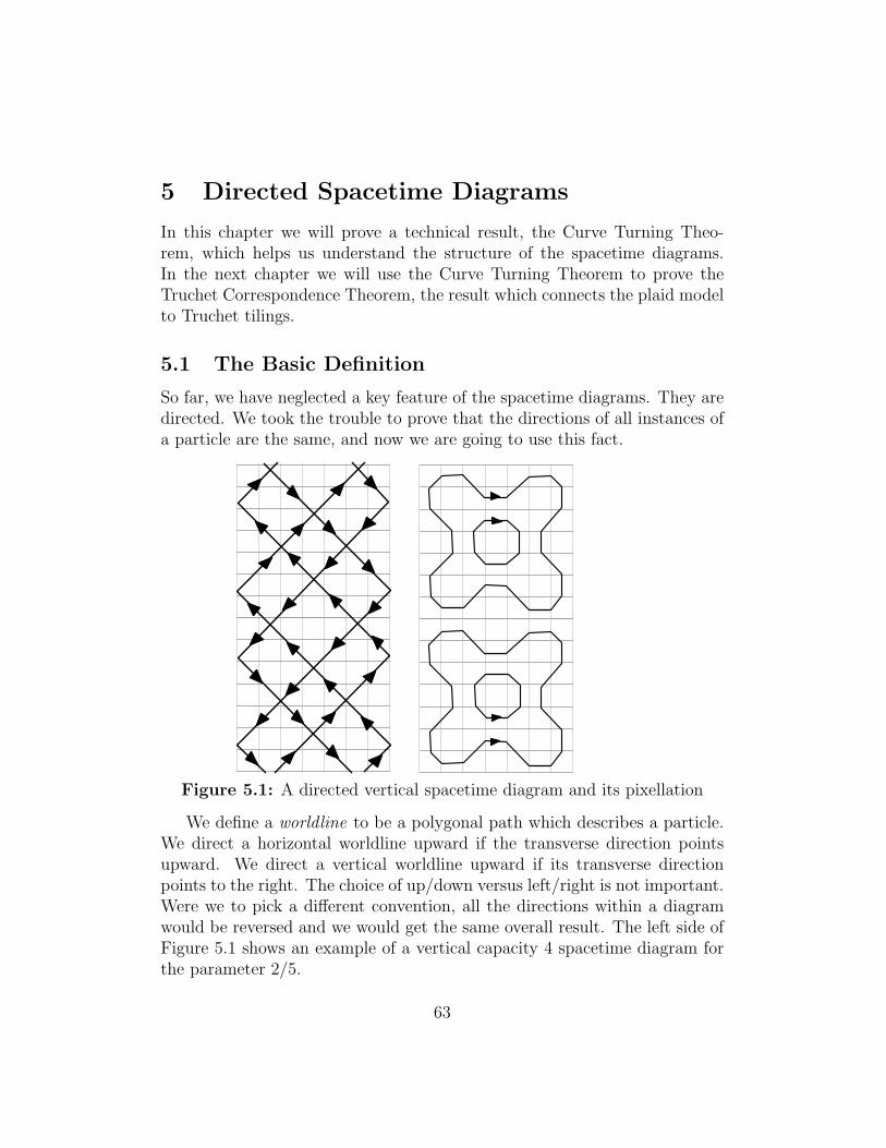
5 Directed Spacetime Diagrams

In this chapter we will prove a technical result, the Curve Turning Theo-rem, which helps us understand the structure of the spacetime diagrams.In the next chapter we will use the Curve Turning Theorem to prove theTruchet Correspondence Theorem, the result which connects the plaid modelto Truchet tilings.

5.1 The Basic Definition

So far, we have neglected a key feature of the spacetime diagrams. They aredirected. We took the trouble to prove that the directions of all instances ofa particle are the same, and now we are going to use this fact.

Figure 5.1: A directed vertical spacetime diagram and its pixellation

We define a worldline to be a polygonal path which describes a particle.We direct a horizontal worldline upward if the transverse direction pointsupward. We direct a vertical worldline upward if its transverse directionpoints to the right. The choice of up/down versus left/right is not important.Were we to pick a different convention, all the directions within a diagramwould be reversed and we would get the same overall result. The left side ofFigure 5.1 shows an example of a vertical capacity 4 spacetime diagram forthe parameter 2/5.

63

5.2 The Curve Turning Process

The right side of Figure 5.1 shows the pixellation of the left side. In thiscase, the pixellation process has an alternate description: We follow alongthe directed segments of the diagram and turn at every intersection. Wecall this the curve following process . Technically, we do not trace directlyon top of the curves, but rather move slightly so that the paths we drawconnect up the centers of the unit integer squares. In Figure 5.1 the curveturning process and the pixellation process produce the same result. This isno coincidence.

Theorem 5.1 (Curve Turning) For any even rational parameter p/q andany capacity κ ∈ 2, 4, ..., 2p, let Σ be any of the corresponding directedspacetime diagrams of capacity κ. Then the pixellation process and the curveturning process produce the same set of polygons.

One reason we are interested in this result is that we will use it to establishthe connection between the plaid model and the Truchet tile system. Thesecond reason is that the Curve Turning Theorem points out the hiddenrobustness of our spacetime surfaces. The pixellation process looks like it isvery delicate. If we jiggle the lines a bit, perhaps we get a completely differentpattern. On the other hand, the curve-following process is quite robust. Itonly depends on the topological pattern in which the directed lines intersect.(Compare Figure 6.3 in the next chapter.) Here is a sample corollary.

Corollary 5.2 The following is true for any even rational parameter. Thereis only one plaid surface in the undirected spacetime model which intersectsthe capacity 2 slices, and this surface intersects each slice in a single polygon.

Proof: The corresponding directed spacetime diagram contains two directedpolygonal paths. Within each block, the corresponding light points corre-spond to a single directed plaid polygon and hence have opposite directions.Thus, we get the same picture as on the right hand side of Figure 5.1. Bythe Curve Turning Theorem, the corresponding pixellated spacetime diagramalways has 2 translation-equivalent loops. When we consider the undirectedmodel, these loops are identified. The polygon from §3.1 intersects all 4 ca-pacity 2 slices and so the same surface intersects all the capacity 2 slices. ♠

64

Remarks:(i) Corollary 5.2 allows us to say that there is a fundamental surface, foreach parameter, in the undirected spacetime diagram. It is the surface whichintersects the lowest capacity slices. This points out some additional signif-icance of the fundamental polygon from §3.1. It is the bottom slice of thefundamental surface.(ii) A somewhat more sophisticated analysis would show that the pattern ofintersection for the capacity 4 slices is always as in Figure 5.1 for any pa-rameter p/q with p ≥ 2. Thus, the union of plaid surfaces in the undirectedmodel intersects the capacity 4 slices in two nested polygons. The outernested polygon is always a slice of the fundamental surface. See Theorem6.2.

5.3 Two Exclusion Principles

The material in this section is preliminary to the proof of the Curve TurningTheorem. We work with the directed plaid model.

Lemma 5.3 (Exclusion I) A unit integer line segment cannot contain twolight points having opposite types and the same directions.

Proof: Call the points ζ1 and ζ2. Consider the vertical case. Suppose ζ1lies on a slanting line of slope −P and ζ2 lies on a slanting line of slope−Q. Define the separation between two light points on the same vertical lineto be the distance between the centers of the vertical unit integer segmentscontaining them. Let ζ ′1 be the reflection of ζ1 in the horizontal midline ofthe relevant block. By symmetry, ζ ′1 and ζ1 have opposite directions. Theseparation between ζ ′1 and ζ1 is even, by symmetry. So, it suffices to provethe separation between ζ ′1 and ζ2 is odd.

ζ ′1 and ζ2 have opposite signs and both lie on slanting lines of the samenegative slope. Hence, their distance is the same as the distance betweenthe y-intercepts of these two slanting lines. By the argument in Lemma 1.3,the distance between these two y-intercepts is an odd integer. Hence, theseparation between ζ ′1 and ζ2 is odd.

In the horizontal case, ζ1 lies on slanting lines of slope ±P and ζ2 linesof slope ±Q. Let (m + 1/2, y) denote the midpoint of the horizontal unitsegment containing ζ1 and ζ2. By symmetry it suffices to consider the case

65

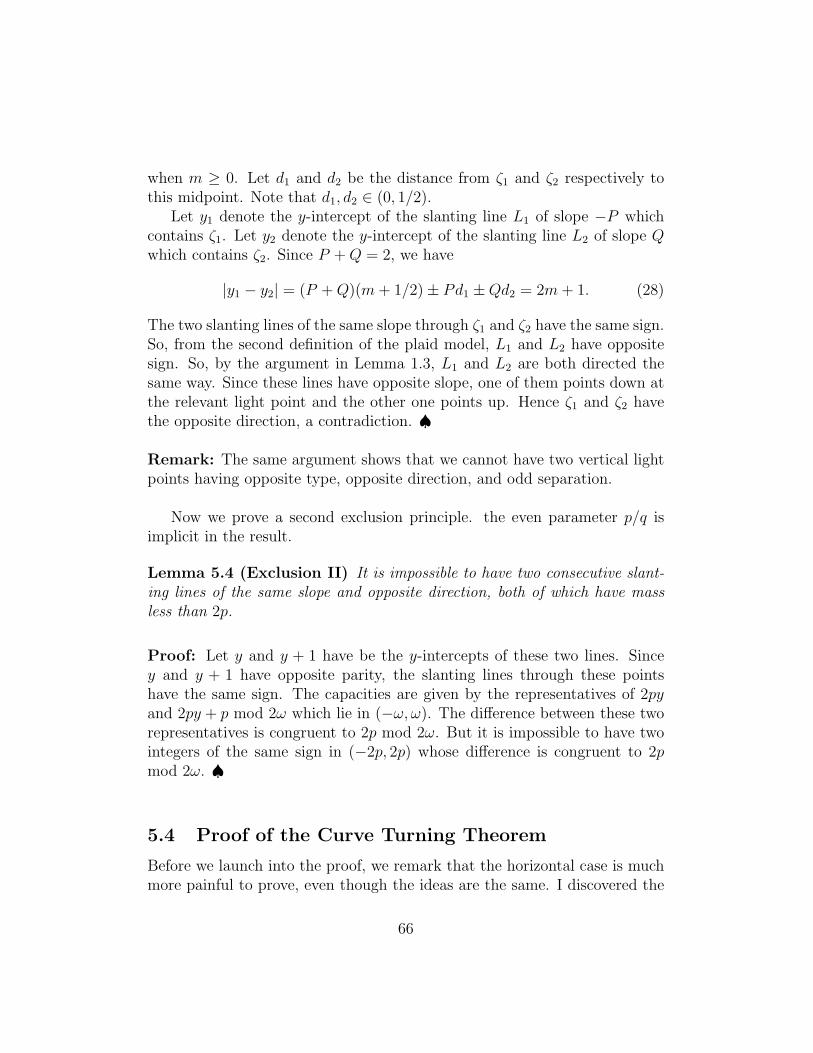
when m ≥ 0. Let d1 and d2 be the distance from ζ1 and ζ2 respectively tothis midpoint. Note that d1, d2 ∈ (0, 1/2).

Let y1 denote the y-intercept of the slanting line L1 of slope −P whichcontains ζ1. Let y2 denote the y-intercept of the slanting line L2 of slope Qwhich contains ζ2. Since P +Q = 2, we have

|y1 − y2| = (P +Q)(m+ 1/2)± Pd1 ±Qd2 = 2m+ 1. (28)

The two slanting lines of the same slope through ζ1 and ζ2 have the same sign.So, from the second definition of the plaid model, L1 and L2 have oppositesign. So, by the argument in Lemma 1.3, L1 and L2 are both directed thesame way. Since these lines have opposite slope, one of them points down atthe relevant light point and the other one points up. Hence ζ1 and ζ2 havethe opposite direction, a contradiction. ♠

Remark: The same argument shows that we cannot have two vertical lightpoints having opposite type, opposite direction, and odd separation.

Now we prove a second exclusion principle. the even parameter p/q isimplicit in the result.

Lemma 5.4 (Exclusion II) It is impossible to have two consecutive slant-ing lines of the same slope and opposite direction, both of which have massless than 2p.

Proof: Let y and y + 1 have be the y-intercepts of these two lines. Sincey and y + 1 have opposite parity, the slanting lines through these pointshave the same sign. The capacities are given by the representatives of 2pyand 2py + p mod 2ω which lie in (−ω, ω). The difference between these tworepresentatives is congruent to 2p mod 2ω. But it is impossible to have twointegers of the same sign in (−2p, 2p) whose difference is congruent to 2pmod 2ω. ♠

5.4 Proof of the Curve Turning Theorem

Before we launch into the proof, we remark that the horizontal case is muchmore painful to prove, even though the ideas are the same. I discovered the

66

tedious proof in the horizontal case after a hard struggle. The vertical case issufficient to establish a connection between the plaid model and the Truchettile system, and one could view the horizontal case as icing on the cake. Forbetter or worse, here is the proof of both cases.

It never happens that there are two directed segments in Σ which arewithin 1 unit of each other, parallel, and pointing in opposite directions.Such segments would correspond to particles having some instances whichlie on consecutive slanting lines of the same negative slope and oppositedirections, and this would contradict the Exclusion Lemma II. The existenceof such lines is the only say it can happen that the pixellation process givestiles which have more than one connector in them. So, the pixellated tileshave at most 1 connector in them.

Since there is only one connector in each tile, the situation is easy toanalyze in a unit square which only has one worldlike going through it. Inthis case, the intersection of the worldline can be moved by at most

√2/2

pointwise so that it matches the pixellated version.We just have to worry that the two processes do opposite things at an

intersection point. First consider the case when two up-pointing worldlinesintersect, as shown in Figure 5.2.

Figure 5.2: two worldlines intersecting

67

Of the two possibilities shown in Figure 5.2, the one on the right is ruledout by the Exclusion Lemma 1. So, for intersections between up-pointingworldlines, the two processes yield the same results. The same goes for theintersection of two down-pointing worldlines.

Now consider the case when the worldlines intersect and are pointingin opposite directions. The picture would look like one of the two optionsin Figure 5.2 except that one of the lines would be pointing in the otherdirection. In this case we want to rule out the case on the left hand sideof Figure 5.2. Consider the case of vertical slices first. If the right handpicture occurs, then we have two light points on the same vertical grid linewhich which occupy adjacent unit integer squares. In terms of the proof ofthe Exclusion Lemma I, we would have two points of opposite type, oppositedirection, and odd separation. This impossible. See the remark following theproof of the Exclusion Principle I.

The horizontal case is more subtle. We will prove that two oppositepointing worldlines intersect on the vertical midline of a unit square withinP/2 from the a horizontal boundary H of the square. (Compare the left handside of Figure 5.1.) This forces H to intersect both worldlines, and again weget the right hand side option.

Our analysis of the particles in §4.1 shows that every horizontal particlehas an instance which lies in the boundary of a block. Hence, the worldlinesin a horizontal slice all intersect the left and right edges of the rectangle atinteger points. Let k denote the difference between the y-coordinates of thepoints where the lines intersect the left edge, as shown in Figure 5.3. (Wehave k = 5 in the figure.)

If k is even then the two worldlines cross on a vertical unit integer segment.If k is odd, then the two worldlines cross on the vertical midline of a unitinteger square, as desired. We rule out the even case. If k is even, then thereare two light points, both lying at the edges of their respective blocks, whosedifference is a vector of the form (2ℓω, 0) for some even integer ℓ. Thesepoints are light points on on a horizontal lines of the same height, and hencethey have the same sign. On the other hand, these points differ by a vectorof the form (2ℓω, 0). Being at the edge of their blocks, they lie on slantinglines of all types. In particular, they each lie on slanting lines of slope −Pwhose y-intercepts differ by 2ℓωP = 4pℓ, an even number. But then our twolight points have the same direction. This contradicts the worldline picture,in which the points have opposite direction.

68

Pk/2

Qk/2

k

Figure 5.3: two worldlines intersecting

Now we know that k is odd as desired, and we come to the final point.The distance between the y-coordinate of the intersection of the two worldlines and the top point on the left in Figure 5.3 is Pk/2. This comes fromthe fact that P + Q = 2 and that the two worldlines have slopes P and Q.We just need to show that

(Pk/2)1 ∈ (−P/2, P/2). (29)

Here (y)1 denotes the difference between y and the integer nearest to y. SinceP = 2p/ω, Equation 29 is equivalent to

(2pk)2ω ∈ (−2p, 2p). (30)

The light points ζ1 and ζ2 in the directed plaid model corresponding tothe two left endpoints in Figure 5.3 differ by the vector (kτω,±ω). Hence,the y-intercepts of the slanting lines of slope −P containing ζ1 and ζ2 differpoints differ by 2kτp ± ω. These points have the same sign and mass in(0, 2p). Given the definition of sign and mass, this forces

(2p× (2pkτ ± ω))2ω ∈ (−2p, 2p).But

(2p× (2pkτ ± ω))2ω = (2p× 2kτ)2ω = (2pk × 2pτ)2ω = (2pk)2ω.

The last equality comes from the fact that 2ptau ≡ 1 mod ω. This completesthe proof.

69

6 Connection to the Truchet Tile System

6.1 Truchet Tilings

In this section we describe the Truchet tilings in [H] with α = β, whereα = p′/q′ ∈ (0, 1/2]. We insist that p′ is odd and q′ is even. We will see thatevery such tiling appears infinitely often as a pixellated spacetime diagram.Figure 6.1 shows the two Truchet tiles having “slope” +1 and −1.

Figure 6.1: The truchet tiles.

The tilings in [H] corresponding to the parameters α, β are described atthe beginning of §3 of [H]. In general, the definition of the tiling depends onsome choice of offset (x, y) ∈ R2, but when α and β are rational, all offsetsgive the same tiling up to translation. We take α = β and x = y = −α/2.The functions ω and η in [H] are the same function.

Following [H], but using our notation, we define η : Z → −1, 1 to bethe sign of

(mα− α/2)1. (31)

In other words, we take the sign of the representative of mα − α/2 mod 1in (−1/2, 1/2) This quantity is never 0, and the sequence is periodic withperiod q′. We call this sequence the Truchet sequence. We call the finitesubsequence η1, ..., ηq′ the first period .

Here are some examples.

• When α = 1/2, the sequence ηm is given by +− repeating

• When α = 1/4 the sequence is + +−− repeating.

• When α = 3/8 the sequence is +−−+−++− repeating.

We define a tiling of the plane in which the Truchet tiles are centered atinteger points (m,n) and the slope of the Truchet tile is the same sign asηmηn. Figure 6.2 shows one period of the periodic Truchet tiling producedby these parameters.

70

+ -

+

-

+

+

+

+ -

-

-

-

+ ++ +- - - -

+

+

+

+

-

-

-

-

Figure 6.2: Truchet tile patterns for α = 1/2, 1/4, 3/8.

The first period of the Truchet sequence has the form (+A)(−A) whereA is a palindrome. The first step in proving this this is to write f(m) =mα− α/2 and observe that

f(m) + f(q + 1−m) = p, f(q/2 +m)− f(m) = p/2. (32)

Given the structure of our sequence, we can always isolate a diamond shapedfundamental domain whose boundary is an impenetrable barrier disjoint fromall Truchet paths. Hence, all Truchet paths are loops, and the picture alwayslooks qualitatively like Figure 6.2.

71

6.2 The Truchet Comparison Theorem

Now for the moment of truth: We can interpret the Truchet tile systems asthe output of curve following dynamics. We direct the vertical line x = mupward if ηm = 1 and downward if ηm = −1. We direct the horizontal liney = n rightward if ηn = 1 and leftward if ηn = −1. When we do the curveturning process and then omit the vertices which go through the centers ofthe squares, we recover the Truchet tiling. This is a purely local result, andeasy to see from a single example. This fact is the basis for our main resultbelow.

Let Γ : R→ R denote the infinite dihedral group generated by the mapsx→ x− 1 and x→ 1− x. A fundamental domain for the action of Γ is theinterval [0, 1/2). Given any x ∈ R, let D(x) denote the representative of Γxin the fundamental domain. The map D plays an important role in [H].

Given a parameter p/q we define

α(p/q) = D(P−1) = D(p+ q

2p

). (33)

For instance,

α(4/9) = D(13/8) = 3/8, α(4/15) = D(19/8) = 3/8.

We chose this example because we have already drawn the Truchet patternfor α = 3/8. Figure 6.2 shows half of the pixellated spacetime diagram forthe vertical slice of capacity 8 = 2× 4.

Figure 6.3: The vertical capacity 8 diagrams the parameter 4/9 and 4/15.

72

Figures 6.2 and 6.3 illustrate our main result. Notice the similarity be-tween the Truchet pattern for 3/8 = α(4/9) = α(4/15) and the capacity 8spacetime diagrams for 4/9 and 4/15.

Before we state our main result, we need one more notion. Within aTruchet tiling, we say that two curves kiss if they intersect the same Truchettile. Within a pixellated spacetime diagram, we way that two polygons kiss ifthe corresponding orbits of the strict curve turning process meet at a vertex.The strict process traces over the curves exactly. Here is our main result.

Theorem 6.1 (Truchet Comparison) Let p/q ∈ (0, 1) be an even ratio-nal parameter. Then the union of curves in the pixellated spacetime diagramof capacity 2p for the parameter p/q is isotopic to the union of curves intwo consecutive fundamental domains for the Truchet tiling associated to theparameter α(p/q). The isotopy preserves the kissing relation.

Remarks:(i) Looking at Figure 6.3, we see that the figures have 8-fold dihedral sym-metry. In the vertical case this always seems to be true, though our proofwill only reveal an 8-fold combinatorial symmetry.(ii) As is pointed out in [H], the polygons in the Truchet pattern can be2-colored so that kissing polygons have opposite colors. When the curvesare equipped with the coloring, the fundamental domain needs to be twiceas large. The same remarks apply to the kissing polygons in the spacetimediagrams.

Before proving the Truchet Comparison Theorem, we derive a corollary.Note, in Figure 6.3, that the largest polygon in each figure completely fills thesquare in which is is drawn. This is true in general, and is a consequence ofthe Truchet Comparison Theorem, because the corresponding polygon in theTruchet system always kisses its translates on all 4 sides. In particular, thislargest polygon intersects every integer Y Z slice in the undirected spacetimemodel except the mirrored boundaries.

Which surface could this largest polygon in the spacetime diagram belongto? Since the polygon intersects the ZY slices of capacity 2, and only thefundamental surface intersects this slice, we see that our polygon must lieon the fundamental surface. Hence, the fundamental surface intersects everynon-boundary Y Z slice in the undirected spacetime model. At the sametime, our polygon intersects every integer XY slice except for one, the slice

73

corresponding to the bottom/top of the diagram. This slice turns out to bethe block B(ω−1)/2, the one which has 4 fold dihedral symmetry. We call thisXY slice the symmetric slice.

The same thing holds in the horizontal case, and this shows that thefundamental surface intersects every nonboundary XZ integer slice as well.Summarizing the argument above, we have the following result.

Theorem 6.2 (Filling) For every even rational paramter, the fundamentalplaid surface intersects every non-boundary integer coordinate slice in theundirected spacetime plaid model except perhaps for the symmetric slice.

Remark: It can happen that the fundamental surface misses the symmetricslice. Figure 4.8 illustrates this for the parameter 1/2. More generally, thishappens for all parameters of the form 1/q and 1 − 1/q. However, it seemsthat usually the fundamental surface does intersect the symmetric slice. Thissituation corresponds to the big polygon in the horizontal slice of capacity2p slopping over the top and bottom of the square when it is drawn in themost symmetric way. Figure 6.4 shows this in action.

Figure 6.4: The vertical capacity 8 diagrams the parameter 4/9 and 4/15.

The rest of the chapter is devoted to the proof of the Truchet ComparisonTheorem.

74

6.3 A Result from Elementary Number Theory

The Truchet Comparison Theorem relies on a curious result from elemen-tary number theory. Let p/q be an even rational parameter. As usual, letω = p+q and τ be such that 2pτ ≡ 1 mod ω. We will carry along an exampleto help explain the result. In the example, p/q = 5/8. This gives ω = 13 andτ = 4. Consider the following sequences.

Red Sequence: Define Ak = ±1 according to the sign of the represen-tative of (ω/2 − ωk) mod 2p that lies in (−p, p). This is the red sequence.In the example, the sequence of representatives is (3/2, 9/2,−5/2, 1/2, 7/2)and the red sequence is + +−++.

Blue Sequence: Take the numbers τ, 3τ, 5τ, ..., (2p − 1)τ mod ω and sortthem so that they appear in order. Call the resulting sequence yk. Wedefine Bk = +1 if yk is even and Bk = −1 if yk is odd. The blue sequenceis Bk. In the example, the unsorted sequence is 4, 12, 7, 2, 10. The sortedsequence is 2, 4, 7, 10, 12. The blue sequence is + +−++.

Lemma 6.3 The red and blue sequences coincide.

Proof: Let 〈m〉p denote the representative of m mod p that lies in 1, ..., p.Let 〈m〉2p denote the representative of m mod 2p in −p+ 1, ..., p.

Let c1, ..., cp ∈ 1, ..., p be such that

yk ≡ τ(2ck − 1) mod ω, k = 1, ..., p. (34)

We will derive the following formula:

ck = pyk +ω + 1

2− ωk. (35)

If we introduce the convention that the sign of 0 is −1 then Ak is always thesign of

ck =⟨ω + 1

2− kω

⟩2p. (36)

From Equation 35 and the fact that ck ∈ 1, ..., p we see that when yk iseven (respectively odd) we have ck = ck (respectively ck = ck − p.) Hence ykis even if and only if Ak = +1. ♠

75

To finish the proof of Lemma 6.3 we establish Equation 35. For ease ofnotation let τ = τ . When p = 1 we have c1 = 1 and y1 = (ω + 1)/2. So, theformula holds. Henceforth assume that p ≥ 2.

We set y0 = 0 and c0 = 0 for notational convenience. Define

δk = ck+1 − ck, ∆k = yk+1 − yk. (37)

Lemma 6.4 |∆i −∆j| ≤ 1 for all i, j.

Proof: Suppose ∆i ≤ ∆j − 2. Let

c′j+1 = cj + δi + ǫp.

Here ǫ ∈ −1, 0, 1 is chosen so that c′j+1 ∈ 1, ..., p. This is always possiblebecause all the c variables are in 1, ..., p. Since 2τp ≡ 1 mod ω,

y′j+1 ≡ τ(2c′j+1 − 1) ≡ τ(2cj − 1) + ∆i + ǫ = yj +∆i + ǫ mod ω.

But then yj ≤ y′j+1 < yj+1. Since yj and yj+1 are consecutive, y′j+1 = yj . But

then ∆i = 1, which means that 2τδi ≡ 1 mod ω. But this forces δi ≡ p modω. If i > 0 this is impossible because ci 6= ci+1 ∈ 1, .., p. If ∆0 = 1 theny1 = 1. But then τ(2c1 − 1) ≡ τ(2p) mod ω for some c1 ∈ 1, ..., p. This isalso impossible. ♠

Lemma 6.5 ω/2 < p∆k < 3ω/2 for all k = 0, ..., p− 1.

Proof: It is convenient to set yp+1 = ω + 1. Observe that for each yi thereis some other yj such that yi + yj = ω+1. But then ∆p = ∆0. We also have

ω + 1 = yp+1 =

p∑

k=0

∆k. (38)

Let ∆ be the min of ∆j and let ∆ be the max. If ∆ = ∆ then the commonvalue is (ω + 1)/(p+ 1) and the inequalities are obvious.

Otherwise, we have ∆ = ∆ + 1, by the previous result. For the upperbound, we have ∆ ≤ ω/(p+ 1), and this gives

p∆ = p∆+ p <p

p+ 1(ω) + p < 3ω/2.

76

For the lower bound we have ∆ ≥ (ω + 2)/(p+ 1), and this gives

p∆ ≥ p

p+ 1(ω + 2)− p = p(q + 1)

p+ 1> ω/2.

A bit of calculus establishes the last inequality for 1 < p < q. ♠

Let c∗k denote the right hand side of Equation 35. We want to show thatc∗k = ck. Using 2τ ≡ 1 mod ω, we compute that c∗k ≡ ck mod ω. Also, Lemma6.5 tells us that

c∗1 = y1 +ω + 1

2− ω = ∆0 +

ω + 1

2− ω ∈ (0, ω).

Since c1 ∈ (0, ω) as well, we must have c1 = c∗1.Suppose by induction that ck = c∗k. Then

c∗k+1 − ck+1 = (c∗k+1 − c∗k)− (ck+1 − ck) = (p∆k − ω)− δk ∈ (−ω, ω).

The last entry of this equation comes from the fact that |δk| ≤ p < ω/2, andfrom Lemma 6.5. Since c∗k+1 ≡ ck+1 mod ω and since |c∗k+1 − ck+1| < ω, wemust have c∗k+1 = ck+1. This completes the induction step. The establishesEquation 35.

6.4 Proof of the Truchet Comparison Theorem

We will give the proof for the spacetime diagrams corresponding to the slicesof positive sign. The other case follows from symmetry.

There are 2p integers 0 < y1 < ..., y2p < 2ω such that the slanting lineshaving these y-intercepts have positive sign and mass less than 2p. We callthis the low mass sequence.

Lemma 6.6 The sequence of directions of the low mass sequence coincideswith the first period of the Truchet sequence, up to a global sign.

Proof: This is an application of the fact that p/q is a good parameter, sothat the red and blue associated sequences coincide. Let α = α(p/q). Let(+A)(−A) be the first period of the Truchet sequence associated to α. LetAk be the first half of this first period.

77

Let yk be the first half of the low mass sequence. This sequence isobtained exactly as the same-named sequence discussed in connection withthe red sequence above. All the slanting lines in question have the same sign,and so their directions are determined by their parities. (See Lemma 1.3.)Therefore, up to a global sign, the sequence of directions of the first half ofthe low mass sequence is the red sequence associated to the parameter. Tofinish the proof we just have to recognize the first half of the first period ofthe Truchet sequence as the blue sequence associated to the parameter. Thefact that the second halves agree follows from symmetry.

Let [x]s denote the sign of (x)s. Let Ak denote the first half of thefirst period of the Truchet sequence. The sequence associated to α + 1 is(+A)(−A) and the sequence associated to 1 − α is (−A)(+A). Hence, ifD(α) = D(α′) then the associated Truchet sequences agree up to a globalsign. Since D(P−1) = α, we see that

Ak = [P−1k − P−1/2]1.

Multiplying through by 2p we get ±Ak = [ωk−ω/2]2p. The sign out in frontis a global one. Hence the first half of the first period of the Truchet sequenceagrees with the blue sequence. ♠

Consider the vertical case of the Truchet Comparison Theorem. To com-pare the pixellated spacetime diagrams to the Truchet tilings, we first extendthe spacetime diagrams so that they fill the whole plane. We track the par-ticles not just in the fundamental blocks but in the entire plane. This is tosay that we consider the light points not just on the segment of a verticalgrid line contained in a block, but on the entire line, and also we repeat thefundamental period endlessly. By symmetry, this extended picture is sim-ply the orbifold universal cover of the original diagram. That is, we extendin the vertical direction by translations and in the horizontal direction byreflections. Figure 6.5 shows how we have reflected the original spacetimediagram in Figure 5.1 across one of its mirrored boundaries. Note how thedirections match.

78

Figure 6.5: Two consecutive fundamental domains

Once we make the extension, the worldlines naturally fit together to makean infinite grid of directed lines of slope ±1. The lines of slope +1 intersectany given horizontal line in our diagram in the same positions that the slant-ing lines of slope −P intersect the corresponding vertical grid line. The linesof slope −1 intersect the same horizontal line at the points where the slantinglines of slope −Q intersect the corresponding vertical lines.

Note that the slanting lines of a given type intersect any vertical line in thesame order as their y-intercepts. Indeed, the pattern of intersection in anyvertical line is the same, up to translation, as the pattern of intersection onthe y-axis. Therefore, assuming the detail above, the sequence of directionsassociated to the lines of slope +1 in the extended spacetime diagram is thesame as the Truchet sequence, up to a global sign change. The same goesfor the lines of slope −1.

Given that the Truchet tiling can also be described in terms of curveturning, we see that the extended pixellated spacetime diagram is isotopicto the Truchet tiling in a way which preserves the kissing relation. The onlydifference is that we have turned the picture 45 degrees and also adjusted the

79

spacing between the lines. (Unlike in the Truchet tiling, the spacing is notalways the same between different pairs of lines in the spacetime diagram.)Moreover, the original spacetime diagram contains 2 consecutive fundamentaldomains for the extended tiling. This completes the proof in the vertical case(modulo the detail), but below we will further analyze the symmetry of thesituation.

The proof in the horizontal case is essentially the same. We just describethe differences. The first difference is that the lines in the extended space-time model have slopes P and −Q rather than 1 and −1. This doesn’t makeany difference from a combinatorial point of view. Second, while the orderin which the slanting lines intersect a given horizontal line is the same as they-intercepts, the two sets are not translation equivalent. They are related byan affine transformation. This does not make any difference. This completesthe proof of the Truchet Comparison Theorem

Remark: Our argument incidentally proves that the horizontal and verticalpixellated spacetime diagrams of capacity κ are combinatorially isomorphicto each other for all κ ≤ 2p. The point is that both diagrams come from thecurve turning construction, and in both slices we see the same combinatorialstructure to the directions of the lines involved.

6.5 Symmetry of the Horizontal Diagrams

Now we discuss the extra symmetry. In the horizontal case, reflection in thevertical midline of the symmetric block B(ω−1)/2 permutes all the horizontalsegments comprising the horizontal slices of the spacetime diagram, and alsopermutes the particles on these lines, preserving the directions. In the space-time diagram this symmetry manifests itself as a rotation about the centerpoint of the horizontal segment corresponding to the symmetric block.

Note furthermore that the spacetime diagram always has 2-fold trans-lation symmetry. Translation by (0, ω) preserves all lines and reverses thedirections. Combining the rotational and translation symmetry, we see thatactually there are 4 points of rotational symmetry in the diagram, evenlyspaced along the vertical midline. If we display the spacetime diagram sothat the bottom line corresponds to the symmetric block, and we just showthe bottom half, one of the centers of rotation is the center of the picture.This is why the examples in Figure 6.4 have 2-fold rotational symmetry.

80

Remark: This analysis works for all the horizontal spacetime diagrams.They all have this rotational symmetry.

The big polygon in the bottom half of the pixellated spacetime diagram– the one discussed in connection with the Filling Theorem – kisses the bigpolygon in the top half, because this is what we know happens in the Truchettiling. But then the big polygon misses at most one horizontal line, as wehave mentioned above. The symmetry we have just discussed shows thatthe missed horizontal segment, assuming it exists, must correspond to thesymmetric block. Again, as we remarked above, this happens rarely.

6.6 Symmetry of the Vertical Diagrams

Reflection in the horizontal midline of any block permutes the light pointsand reverses the directions. This symmetry manifests itself as a reflectionsymmetry in the vertical midline of the spacetime diagram. This analysisworks for any capacity. All these diagrams have vertical bilateral symmetry.

We have already remarked in the proof of Lemma 6.5 that for each yithere is some yj such that yi + yj = ω+1. Since this numbers are sorted, wemust have j = p+ 1− i. In short,

yk + yp+1−k = ω + 1, k = 1, ..., p. (39)

This means that (0, y) has positive sign and mass less than 2p if and only if(0, ω+ 1− y) does. At the same time, the points (0, yp) and (0, ω− yp) havethe same mass and opposite sign. This means that the points of mass lessthan 2p are paired in the sense that each point (0, y) of mass less than 2phas a partner point (0, y± 1) which has opposite sign and mass less than 2p.

In every block, there are two vertical lines of capacity 2p. Each slantingline produces a light point on one of the lines and the partner slanting lineproduces a light point on the other one. Relatively speaking, the two lightpoints are in the same vertical integer segment. They are not actually in thesame unit integer segment, however, because the one point is on the one lineand the other point is on the other.

This structure has a special implication in the symmetric block. Reflec-tion in the vertical midline of the symmetric block permutes the light points.Hence, in the symmetric block, the light points on each vertical segment ofcapacity 2p are paired. There are either 0 or 2 in each vertical unit integer

81

segment. In terms of the spacetime diagram, this means that all the linesof slope +1 quasi-meet all the all the lines of slope −1 in the correspondinghorizontal slice: Both lines deposit light points in the same intervals. Takea hard look at the bottom of Figure 5.1. The lines do not meet preciselyon the bottom line, but they meet up to one unit, and inside the same unitinteger segments.

The bilateral symmetry of the diagram and the quasi-meeting propertyof the lines implies that reflection in the horizontal slice corresponding tothe symmetric block is an approximate symmetry of the diagram itself andan exact symmetry if the pixellated diagram. The pixellated diagram hasvertical and horizontal bilateral symmetry. Hence it also has the same pointsof reflection symmetry as in the horizontal case.

The same analysis as in the horizontal case now shows that the big poly-gon in each half of the spacetime diagram of capacity 2p can only miss thehorizontal line corresponding to the symmetric block. This time, the quasi-meeting property implies that the big polygon does actually miss the segmentwe are talking about.

Remark: The pixellated vertical spacetime diagrams of all capacities seemto exhibit the same reflection symmetry mentioned above. I think that sim-ilar arguments as the ones given above would establish this. What is harderto understand is that all these diagrams seem to exhibit an exact 4 fold ro-tational symmetry. For the capacity 2p slice, the combinatorial 4-fold sym-metry follows from the Truchet Comparison Theorem, thanks to the exact4-fold rotational symmetry of the Truchet pattern.

82

Part II

The Plaid Master PictureTheorem

83

7 The Plaid Master Picture Theorem

7.1 The Spaces

DefineX = R3 × [0, 1]. (40)

The coordinates on X are given by (x, z, y, P ). We think of

P =2A

1 + A, A = p/q, (41)

but P is allowed to take on any real value in [0, 1]. Define the following affine

transformations of X.

• TX(x, y, z, P ) = (x+ 2, y + P, z + P, P ).

• TY (x, y, z, P ) = (x, y + 2, z, P );

• TZ(x, y, z, P ) = (x, y, z + 2, P );

Define two abelian groups of affine transformations:

Λ1 = 〈TX , TY , TZ〉, Λ2 = 〈T 2X , TY , TZ〉. (42)

Finally defineXk = X/Λk, k = 1, 2. (43)

The space X2 is a double cover of X1. Both spaces should be consideredflat affine manifolds - i.e. manifolds whose overlap functions are restrictionsof affine transformations. All the affine transformations in sight preserve theslices R3 × P and act as translations on these slices. This X1 and X2 arefibered by 3-dimensional Euclidean tori. We denote these tori by X1(P ) andX2(P ) respectively.

Remark: The reason why we keep track of two spaces is that a suitablepartition of X1 into polytopes determines the unoriented polygons in theplaid model whereas a suitable partition of X2 determines the oriented poly-gons in the plaid model. Often it is easier to do computations with X1 eventhough X2 contains more information.

84

7.2 The Partition

Here we describe a partition of the space X1 into convex integral polytopes.Taking the double cover, we get a partition of X2. Lifting to X, we get aΛ1-invariant partition of X into infinitely many polytopes. When we addlabels, this infinite partition is only Λ2-invariant. Our computer programlets the user see the partition in an interactive way.

The rectangular solid[−1, 1]3 × [0, 1]. (44)

serves as a fundamental domain for the action of Λ1 on X. We think ofthis space as a fiber bundle over the (x, P ) plane. The base space B is therectangle [−1, 1] × [0, 1]. The space B has a partition into 3 triangles, asshown in Figure 7.1.

13 24

14

2 3

000WN0000E0000S0

N00000E00W00000S

0N0000W0000SE000

x

P

Figure 7.1: The (x, P ) base space.

Each triangular region has been assigned a 4 × 4 matrix which we willexplain momentarily. The slices above each open triangle in the partition ofB consists of a 4×4 grid of rectangles. For of the rectangles, corresponding tothe polytopes labeled by the emptyset are squares. (In Figure 7.2 we replacethe emptyset by the symbols S,W,N,E because this makes the rest of thelabeling pattern more clear. The pattern of the squares is indicated by thenonzero entries in the matrices. For instance, the grid shown in Figure 7.2corresponds to a fiber over the left triangle. We have also indicated the labelsin the picture.

85

W

N

E

SSN SE SW

ES

NS

WS

EN

WN WE

NE NW

EW

Figure 7.2: The checkerboard partition

The labels can be derived from the matrices in Figure 7.1. Every non-square rectangle in a column has the same first label and every rectangle ina row has the same second label.

The edge labels in Figure 7.1 encode degenerations in the fibers. Awayfrom the singular edges of the base space, each polytope is a rectangle bundleover an open triangle. As one approaches the edges of the triangles in thebase, the partition degenerates in that some of the rectangles shrink to linesegments or points. The numbers on the edges in Figure 7.1 indicate whichrows and columns degenerate. For instance, as we approach the edge labeled2, the thickness of second column from the left tends to 0 and at the sametime the thickness of the second row from the bottom tends to 0. The whole(unlabeled) picture is symmetric with respect to reflection in the line y = x.

From the description of these degenerations and from the fact that weknow we are looking at slices of convex integral polytopes, one can actuallyreconstruct the entire partition from the labelings in Figure 7.1. Each poly-tope in Figure 7.2 comes with a label. For instance, the label of the polytopewhich intersects the fiber in the northwest corner is W,N.

Thus, each polytope in the partition of X either is either labeled by the

86

∅ symbol, or else by a pair A 6= B, where A,B ∈ N,E,W, S. Now weexplain how we enhance the labeling so that each polytope not labeled by∅ is labeled by an ordered pair (A,B). Our idea is to explicitly give theordering on a list of 10 polytopes (below) and then use the action of Λ1 topropagate the ordering to the whole partition. The group Λ2 preserves theordered labeling and elements of Λ1−Λ2 reverse the ordering. We found theordered labeling (which turns out to be canonical) by trial and error.

Here we list the vertices and ordered labels of 10 polytopes. All thepolytopes in the partition of X can obtained from these using the groupgenerated by Λ1 and the following two additional elements:

• Negation: The map (x, y, z, P )→ (−x,−y,−z, P ) preserves the par-tition and changes the labels as follows: N and S are swapped and Eand W are swapped.

• Flipping: The map (x, y, z, P ) → (x, z, y, P ) preserves the partitionand changes the labels as follows: N and S are swapped, and the orderof the label is reversed.

The last polytope listed has 12 vertices, and the listing is spread over 2 lines.

−1−1−10

−1+1−10

+1+1−10

+1+1+10

000+1

(W,E)

+1+1−10

+1+10+1

+1+1−1+1

0+1−1+1

00−1+1

(E, S)

+1−1−10

+100+1

+10−1+1

00−1+1

0−1−1+1

(E,N)

−1+1−10

+1+1−10

+1+1+10

000+1

0+10+1

+1+10+1

+1+1+1+1

(W,S)

87

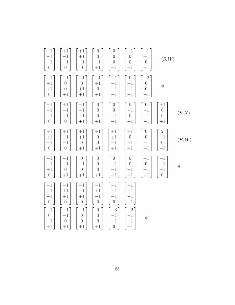
−1−1−10

+1−1−10

+1+1−10

00−1+1

000+1

+100+1

+1+10+1

(S,W )

−1+1+10

−100+1

−10+1+1

−1+10+1

−1+1+1+1

0+1+1+1

−200+1

∅

−1−1−10

+1−1−10

−1−1−1+1

000+1

00−1+1

0−10+1

0−1−1+1

+100+1

(S,N)

+1+1−10

+1−1−10

+1+10+1

+100+1

+1+1−1+1

+10−1+1

00−1+1

2+10+1

(E,W )

−1−1+10

−1−10+1

0−10+1

000+1

0−1+1+1

00+1+1

+10+1+1

+1−1+10

∅

−1−1−10

−1+1+10

−1−1+10

−1+1−10

+1+1+10

−1−1−1+1

−10−1+1

−1−10+1

−100+1

000+1

−3−1−10

−2−1−1+1

∅

88

7.3 The Map

The plaid grid is defined to be the set G of centers of integer unit squares.For each parameter A ∈ (0, 1), there is a linear map ΦA : G→ X, given by

ΦA(x, y) = (2Px+ 2y, 2Px, 2Px+ 2Py, P ), P =2A

1 + A. (45)

In this section we fix A and P = 2A/(1+A) and we write Φ = ΦA. Also,we restrict the action of Λ1 to R3 × P and we identify this slice with R3.Thus, we think of Λ1 as a lattice of translations acting on R3.

Lemma 7.1 Let L1 be the lattice of symmetries of the undirected plaid modeland let L2 be the lattice of symmetries of the directed plaid model. If weinterpret Λj as a lattice of translation vectors, then Φ(Lj) ⊂ Λj for j = 1, 2

Proof: We will prove this for j = 1. The proof for j = 2 is similar. Recallthat A = p/q and P = 2A/(1+A) and ω = p+ q and that L is generated by(ω2, 0) and (0,∞). Since Φ is a linear map, it suffices to prove that Φ(ω2, 0)and Φ(0, ω) both belong to Λ1. We compute

Φ(ω2, 0) = (2Pω2, 2Pω2, 2Pω2) =

Pω2(2, P, P ) + (0, 2Pω2 − P 2ω2, 0) + (0, 0, 2Pω2 − P 2ω2).

Note that P = 2p/ω, so that Pω2 and P 2ω2 are both even integers. Hence,the last two vectors above have the form (0, k, 0) and (0, 0, k) for some eveninteger k. All the vectors on the second line of our equation belong to Λ1.

We compute

Φ(0, ω) = (2ω, 0, 2Pω) = ω(2, P, P ) + (0,−ωP, 0) + (0, , 0Pω).

Again, the last two vectors have the form (0,−k, 0) and (0, 0, k) for someeven integer k. So, all the vectors on the right hand side belong to Λ1. ♠

Recall that Z0 and Z1 respectively denote the set of even and odd inte-gers, we define

X =(Z1

ω,Z0

ω,Z0

ω

). (46)

Note that the lattice Λ1(P ) consists entirely of vectors in (Z0/ω)3. Hence Λ1

preserves X . The quotient X /Λ1 is a finite set of points with ω3 members.The quotient G/L is also a finite set of points with ω3 members.

89

Lemma 7.2 Φ induces a bijection between G/Lj and X /Λj for j = 1, 2.

Proof: We prove this for j = 1. The case of j = 2 is similar, and indeed fol-lows from the case j = 1 and symmetry. Looking at the formula in Equation45, we see that Φ(c) ∈ X . Hence, by Lemma 7.1, the map Φ induces a mapfrom G/L to X /Λ1. In view of the fact that both sets have the same numberof points, we just have to show that the induced map is an injection.

Suppose that Φ(c1) = Φ(c2). We write

c2 − c1 = (x, y) =(mω,n

ω

), m, n ∈ Z. (47)

We have

Φ(c2)− Φ(c2) =(2pmω2

,2pm

ω2− pn

ω2,2pm

ω2− Pn

ω2

)mod Λ.

In order for the first coordinate to vanish mod Λ, we must have m ≡ 0 modω2. For the second and third coordinates to vanish mod Λ, we must haven ≡ 0 mod ω. But then c2 − c1 ∈ L1. ♠

Now we come to the main point in this section.

Lemma 7.3 (Definedness) Φ(G) is disjoint from the boundaries of the

polytopes in the partition of X.

Proof: In view of our previous results, we just need to know that X doesnot hit the boundaries of polytopes in our partition. We forget the lastcoordinate and work in R3. Say that a special plane is a plane of the formT × R2 with T ∈ Z1/ω. By definition, X is contained in the union ofspecial planes.

We check that each special plane intersects the walls of the partition inlines of the form x = u and y = u. When T = −1, the values of u are−1, 1 + P, 1, all of which belong to Z1/ω. As the value of T changes by2/ω, the offsets for the wall-fiber intersections change by ±2/ω. Hence, wealways have u ∈ Z1/ω. But then X does not hit any of these lines.

The proof is done, but we want to elaborate on the picture. If we placea cube of side length 2/ω around each point of X , then these cubes tile R3.Moreover, these cubes intersect each special plane in an ω × ω grid. Theimage Φ(G) intersects this grid at the centers of the squares whereas thewalls of the partition intersect the grid in line segments extending the edgesof the squares. ♠

90

7.4 Three Dimensional Interpretation

We can think of Φ as a map from the set of centers horizontal unit integersquares in the cubical plaid model. In these coordinates, the vector (0, 0, 1)corresponds to (−τ ,±ω). The sign depends on the parity of the z-coordinateof the horizontal slice at which the vector (0, 0, 1) is anchored.

The set of points in R3 corresponding to points in the plaid grid have theform (x, y, z) where x, y are half integers and z is an integer. In this section,we will give a formula for Φ(x2, y2, z2) − Φ(x1, y1, z1) where (x1, y1, z1) and(x2, y2, z2) are two points of this kind.

Lemma 7.4 Let Φ : Z3 → R3/Λ2 be the map given by

Φ(x, y, z) = x(2P, 2P, 2P ) + y(2, 0, 2P ) + z(−2, 0, 0) mod Λ2. (48)

This formula computes

Φ(x1, y1, z1)− Φ(x2, y2, z2)

where (x, y, z) = (x2, y2, z2)− (x1, y1, z1) in the cubical coordinates.

Proof: We have

Φ(1, 0) = (2P, 2P, 2P ), Φ(0, 1) = (2, 0, 2P ). (49)

We also have

Φ(−τω, 0) = (2P τω, 2P τω, 2P τω) = (4pτ , 4pτ , 4pτ) ≡1

(4pτ , 0, 0) ≡2 (0,−2Ppτ ,−2Ppτ) ≡3 (0, P, P ) mod Λ2. (50)

Equivalence 1 comes from the fact that 4pτ ∈ 2Z. Equivalence 2 comes fromsubtracting multiples of (2, P, P ). Equivalence 3 comes from the fact that

−2Ppτ − P = P (−2pτ − 1) = PKω = 2pK ∈ 2Z.

Next, we compute

Φ(0, ω) = (2ω, 0, 2Pω) ≡ (2ω, 0, 0) =

(2(ω − 1) + 2, 0, 0) ≡ (2,−Pω + P,−Pω + P ) ≡ (2, P, P ) mod Λ2. (51)

This combines with Equation 50 to give

Φ(−τ ,±ω) ≡ (0, P, P )± (2, P, P ) ≡ (−2, 0, 0) mod Λ2. (52)

Putting all this together, we get Equation 48. ♠

91

7.5 The Main Result

Once again we fix an even rational parameter A and set P = 2A/(1+A). Weuse the same notation conventions from the previous section. The partitionof X by labeled polytopes descends to partition of X2.

The map Φ : G → X2 determines a tiling of R2, as follows. In the unitinteger square centered at c ∈ G we place...

• the empty tile if Φ(c) lies in a polytope labeled by ∅, or

• the tile with a directed segment pointing from the midpoint of the αedge to the midpoint of the β edge if Φ(c) lies in a polytope with label(α, β).

We call this tiling the directed tiling . Given a unit square and an edgeE of we say that the directed tiling involves (, E) if the connector in uses the midpoint of E. In this case, we call (, E) out-pointing if theconnector points to E and in-pointing if the connector points from E. Hereis our main result, which holds for every parameter.

Theorem 7.5 For any unit integer square and any edge E of , the num-ber light points assigned to E is odd if and only if the directed tiling involves(, E). In this case, (, E) is in-pointing if and only if the transverse direc-tion associated to the light point on E in §1.6 points into .

In short, Theorem 7.5 says that Theorem 1.1 is true, that the tiling ob-tained by the plaid construction matches the tiling obtained from the PET,and that the transverse directions given in §1.6 match the transverse direc-tions given by the PET. There is a complete isomorphism. As an immediatecorollary, the method of assigning directions in §1.6 is tile consistent.

Now we rephrase Theorem 7.5 in terms of the Plaid Master Picture The-orem. Consider the map f : G → G that comes from simply following thearrows on the tiles. Given c0 ∈ G, the new point C1 = f(c0) is defined to bethe center of the tile into which the tile at c0 points. For instance, the tilecentered at c0 is NE, then c1 = c0 + (1, 0). In case the tile centered at c0 isempty, we have c1 = c0.

Thanks to Theorem 7.5, there is a corresponding map F : X → X suchthat

F Φ = Φ f. (53)

The map F has the following definition:

92

• F is the identity on polytopes labeled by ∅.

• F (x, y, z) = (x, y, z) + (2, 0, 2P ) on polytopes whose label ends in N .

• F (x, y, z) = (x, y, z)− (2, 0, 2P ) on polytopes whose label ends in S.

• F (x, y, z) = (x, y, z) + (P, P, P ) on polytopes whose label ends in E.

• F (x, y, z) = (x, y, z)− (P, P, P ) on polytopes whose label ends in W .

We can also interpret F as a map

F2 : X2 → X2 (54)

because everything in sight is Λ2 invariant. With this interpretation, (X2, F2)is the fibered integral affine PET. What we mean is the 4 dimensional systemis piecewise affine, and that the PET preserves the P -slices and acts as anordinary piecewise translation in each fiber. The 4 dimensional system isintegral in the sense that all the polytopes in the partition have integervertices. Thus, Theorem 7.5 implies the Plaid Master Picture Theorem fromthe introduction.

7.6 The Undirected Result

In Part 4 of the monograph, when we prove the Quasi-Isomorphism Theorem,we will simplify our calculations by using the space X1. Accordingly, we sayabout the undirected version of Theorem 7.5. The polytopes which partitionX1 are labeled by unordered pairs of the form N,E, etc. We cannot orderthese pairs in a canonical way because the action of elements in Λ1 − Λ2

reverses the orderings within our labels. Thus, some element of Λ1 − Λ2

maps a polytope labeled (N,E) to a polytope labeled (E,N).Nonetheless, we we can use the unordered labels to define an undirected

tiling in the same way that we defined the directed tiling. We just leave offthe directions. Theorem 7.5 has the following immediate corollary.

Theorem 7.6 For any unit integer square and any edge E of , thenumber light points assigned to E is odd if and only if the undirected tilinginvolves (, E).

Theorem 7.6 is good enough for the proof of the Quasi-Isomorphism The-orem.

93

8 The Images of Particles

8.1 Overview

The next three chapters are devoted to the proof of Theorem 7.5. As always,we fix a parameter A = p/q and set ω = p+ q.

Each particle in the directed model breaks up into two half-particles inwhich the relative motion of the subset goes in one direction across the block.In the horizontal cases, one of the half-particles has 2p consecutive instancesand moves east and the other half-particle has 2q instances and moves west.In the vertical case, one of the half-particles moves south and the other movesnorth. Both half-particles have ω instances in this case.

Let z0, ..., zn−1 be the successive instances of a vertical (respectively hor-izontal) half-particle and let c0, ..., cn−1 be the corresponding sets of centersof the unit squares containing these points on the west (respectively south)edge. We are interested in the image

Z =n−1⋃

i=0

Φ(cj) ⊂ X1(P ). (55)

Our basic result is that the images of half-particles under the classifying maptravel in straight lines . Here is the precise statement. Let (T, U1, U2) becoordinates on this fundamental domain. This chapter is devoted to provingthe following result, which works for both light and dark particles.

Lemma 8.1 (Particle) The following is true.

1. If Z corresponds vertical P particle, then modulo Λ2, the set Z lies ina segment with endpoints (T,−1, U2) and (T, 1, U2).

2. If Z corresponds vertical Q particle, then modulo Λ2, the set Z lies ina segment with endpoints (T, U1,−1) and (T, U1, 1).

3. If Z corresponds horizontal P particle, then modulo Λ2, the set Z lies ina segment with endpoints of the form of the form (±1, U1, U2)−(P, P, P )and (±1, U1, U2) + (P, P, P ).

4. If Z corresponds horizontal Q particle, then modulo Λ2, the set Z is asegment with endpoints of the form of the form (±1, U1, U2)− (Q, 0, 0)and (±1, U1, U2) + (Q, 0, 0).

94

8.2 The Vertical Case

If ck and ck+1 are two successive instances of a vertical P half-particle thenin terms of the 3 dimensional model ck+1−ck = (0, 1, 1). Hence, by Equation48,

Φ(ck+1)− Φ(ck) ≡ (0, 0, 2P ) mod Λ2.

This proves Statement 1.In the vertical type Q case, we have ck+1 − ck = (0,−1, 1). Hence, by

Equation 48,

Φ(ck+1)− Φ(ck) ≡ (−4, 0,−2P ) ≡ (0, 2P, 0) modΛ2.

This proves Statement 2. .

8.3 The Horizontal P Case

Our first result vastly simplifies the amount of calculating we have to do.

Lemma 8.2 If Statement 3 is true for one horizontal P particle then it istrue for all of them.

Proof: This is most easily seen in terms of the 3-dimensional interpretationof the map. All the horizontal P particles have instances of the form (0, y, z)for y, z ∈ N . By Equation 48, the sets corresponding to the two particlesdiffer from each other by a translation of the form (0, y′, z′) or (2, y′, z′). ♠

We will compute using the (dark) half particle which has an instance at(0, 0) in the plane. In terms of the 3-dimensional interpretation of the model,the successive instances z0, ..., z2p−1 are given by

zk = (k/P, 0, k). (56)

See (the gray part of) Figure 4.1.Let x denote the half integer nearest x. We have

x = x− [x] + 1/2, (57)

where [x] is the number in (0, 1) representing x mod Z. These equations arenot defined when x ∈ Z, but this situation does not arise for us.

95

The square center ck corresponding to zk is

(k/P, 1/2, k). (58)

In the two dimensional model, c0 has coordinates (1/2, 1/2). Using theoriginal definition of the map Φ we see that

Φ(c0) = (P − 1, 0, P ). (59)

Note that ck − c0 ∈ Z3, so we may use Equation 48 to compute. Equation48 gives

Φ(ck)− Φ(c0) = (µk, µk, µk) + (−2k, 0, 0) mod Λ2, (60)

whereµk = 2Pk/P − 2P0/P = 2k − 2P [k/P ]. (61)

Settingνk = −2P [k/P ] ∈ [−2P, 0], (62)

, we getΦ(ck)− Φ(c0) ≡ (νk, νk, νk) mod Λ2, (63)

Hence Φ(ck) lies on the line segment with endpoints

(−1 + P, 0, P ), (−1− P,−2P,−3P ). (64)

This proves Statement 3.

8.4 The Horizontal Q Case

The same argument as in Lemma 8.2 reduces this case to the study of asingle horizontal Q particle. We will compute using the (dark) particle which(again) has an instances z1, ..., z2q, where

zk = (k/Q, 0, 2ω − k) (65)

Remark: We are abusing our notation and conventions to make the calcula-tion as clean as possible. First, we are tracing out instances going “backwardsin time”, so that in Figure 4.1 we would be tracing the black worldline fromtop to bottom. Second, we are allowing the third coordinate to lie in [0, 2ω]rather than in [0, ω], as we would want for the undirected model. However,for the purposes of verifying Statement 4 of the Particle Lemma, there is no

96

harm in replacing a point (a, b, c) with the point (a, b, c± ω).

The centers corresponding to our points are

ck = (k/Q, 1/2, 2ω − k, k = 1, ..., 2q. (66)

It is convenient to add c0 to the list of centers.Before we do the calculation, we use the fact that P + Q = 2 to derive

an alternate version of Equation 48.

Φ(x, y, z) = x(−2Q, 0, 0) + y(2, 0,−2Q) + z(−2, 0, 0) mod Λ2. (67)

Again, this only works when x, y, z ∈ Z.We have Φ(c0) = (P − 1, 0, P ) as in the previous case. Using Equation

67, we have

Φ(ck)− Φ(c0) =(− 2Q(k/Q − 0/Q), kQ, kQ

)≡

(2Q[k/Q], 0, 0) mod Λ2. (68)

From this equation we see that Φ(ck) lies in the segment with endpoints

(1−Q, 0, P ) = (P − 1, 0, P ), (1 +Q, 0, P ) = (P − 1 + 2Q, 0, P ).

This proves Statement 4.

Remark: The same remarks about symmetric instances of the particle applyin this case as well.

97

9 Proof of the Main Result

9.1 Symmetric Instances

In the previous chapter we understood the images of half-particles under themap Φ. As in the previous chapter, we suppress the coordinate which recordsthe parameter and we work in R3. In this chapter we will prove the mainresult modulo two lemmas which we prove in subsequent chapters.

We say that a symmetric instance of a half-particle is an instance thatlies in a unit integer square that has its midpoint on the horizontal midlineof a block. Every half-particle has a symmetric instance. If z is a symmetricinstance of vertical (respectively horizontal) particle, let c be the center ofthe unit integer square which has z on its west (respectively south) edge.In this chapter we will study the image of Φ(c). We call this the point thecharacter of z. And we denote it by φ(z). Note that φ(z) = Φ(c).

Remark: In making this definition we have arbitrarily chosen to favor thewest and south edges over the east and north edges. Were we to make theswitch, we’d get similar answers. We will arrange our proof so that we donot need to consider the east and north edges. The point is that every eastor north edge of a square is also a west or south edge of an adjacent square.

Lemma 9.1 Let z be a symmetric instance of a vertical particle. Then modΛ2, the character of z has the form (T, U, U).

Proof: We have c = (x, y) where y = ±ω/2. Note that 2Pω = 2p ∈ 2Z.Hence, Equation 45 gives Φ(c) = (2Px, 2Px, 2Px) + (±ω, 0, 0). ♠

Lemma 9.2 Let z be a symmetric instance of a horizontal particle. Thenmod Λ2, the character of z has the form (±1, U1, U2).

Proof: This time we have c = (x, y) where x = kω/2 for some integer k.Also, 2y is an odd integer. As in the previous result, 2Pkω/2 ∈ 2Z Butthen, by Equation 45, the first coordinate of Φ(c) is an odd integer. Mod 4Zwe can take this coordinate to be ±1. ♠

98

9.2 Sharp Containers

We identify 4 kinds of vertical light points, namely

(P,Q, E,W).For example, the light point of type (P,west) lie on slanting lines of slope −Pwhich are directed so that they point west. Likewise we identify 4 kinds ofhorizontal light points, namely

(P,Q, N,S).These names have similar interpretations. We also classify the dark points,but we ignore the directions. Thus there are horizontal dark points of typeP and Q, and vertical dark points of type P and Q. We say that a dark pointhas the same undirected type as a light point if, when we forget the direction,we get the same type. For instance, a vertical dark point of type P has thesame type as the vertical light points of type (P,east) and (P,east).

We say that a set Σ ⊂ R3 is a container for a given type

1. The character of a light point with the given type always maps into Σmod Λ2.

2. The character of a dark point with the same undirected type nevermaps into Σ mod Λ2.

In this section we make these definitions just for the points which are sym-metric instances of particles. However, in the next section we mean thesedefinitions for all intersection points, light or dark, symmetric or not.

We define the fundamental involution on the space X2 = X/Λ2 to betranslation by (2, P, P ). This map is the identity mod Λ1 and an involutionmod Λ2. Here are the main results of this chapter.

Lemma 9.3 (Vertical) In each vertical case there exists a sharp containerwhich is a disjoint union of 2 triangles in the U1 = U2 plane. For the types(P,east) and (Q,west) the vertices of these triangles are

(−2 + P, 1, 1), (−1 + P, 1, 1), (−2 + P, 0, 0)

and

(P,−1 + P,−1 + P ), (−1 + P,−1 + P,−1 + P ), (P, P, P )

and for the types (P,west) and (Q,east) the triangles are translated by thefundamental involution.

99

Figure 9.1 shows the projection of these sets into the (T, U) plane (foreither U = U1 or U = U2) and for the parameter 2/5. The lightly shadedtriangles correspond to (P,west) and (Q,east) and the darkly shaded trianglescorrespond to (P,east) and (Q,west). Notice that reflection in the point(P, P, P ) swaps these two sets, as does the fundamental involution.

Figure 9.1: The images of vertical symmetric instances

Lemma 9.4 (Horizontal) In each horizontal case there exists a sharp con-tainer which is a disjoint union of two (1, 1,

√2) right isosceles triangles, one

contained in the plane T = −1 and one contained in the plane T = +1. Forthe types (P,north) and (Q,south) the vertices of these triangles are

(1, 1,−1 + P ), (1, 0,−1 + P ), (1, 1, P )

and(−1, 1− P, 1), (−1, 2− P, 1), (−1, 1− P, 0)

and for the types (P,south) and (Q,north) the new triangles are the imagesof the ones above under te fundamental involution.

Figure 9.2 shows the projection of the sets corresponding to (P,north)into the (U1, U2) plane for the parameter 2/5. The sets for (Q,south) are thesame, and the remaining sets are reflected images of these. The dark trianglelies in the T = −1 plane and the light triangle lies in the T = +1 plane.

+Figure 9.2: The images of horizontal symmetric instances

Remark: The reader can see these sets plotted for any smallish parameteron our computer program. Set the main console to “sanity checks” and thechoice to “images by type”.

100

9.3 Prism Structure

Now we combine the Particle Lemma with the results in the previous section.Every directed half-particle has a symmetric instance, so the results in theprevious section apply to every particle. The Particle Lemma combines withthe Vertical Lemma and the Horizontal Lemma to prove the following result.

Lemma 9.5 For every parameter and every type there is a sharp containerwhich is a union of 2 prisms. The vertices of this prism vary linearly withthe parameter. The Λ2 orbit of these prisms consists of an infinite family ofpairwise disjoint prisms.

Proof: A prism is a polyhedron which is affinely equivalent to the productof a triangle and in interval. We will give the proof for the particles oftype (P,north), but the same argument works in general. The container forthe symmetric instances of (P,north) is a union of 2 triangles, one in theplane T = −1 and the other in the plane T = +1. Call this set Σ0. Bythe Particle Lemma we get a sharp container for all the particles of type(P,north) by considering the union of line segments parallel to (1, 0, 0) and oflength 2Q = 4−2P that are centered on Σ. The set of such points is a unionof two prisms. For instance, the prism corresponding to the first triangle inthe Horizontal Lemma has vertices

(1, 1,−1+P )±η, (1, 0,−1+P )±η, (1, 1, P )±η, η = (2−P, 0, 0). (69)

We just take the vertices listed in the Triangle Lemma and add ±η. Theother cases have similar treatments. The crucial fact is that the directiongiven by the Particle Lemma is always transverse to the triangles given bythe Vertical Lemma or the Horizontal Lemma.

In each case, we can see by inspection that the interiors of these prismsembed in X2. Hence, when we take all the pre-images under the coveringmap X → X2 we get an infinite family of prisms having pairwise disjointinteriors. ♠

Remark: In the vertical case the analysis is slightly misleading. Lookingat the Particle Lemma in the vertical case, we see that the picture we getin R3 is actually an infinite union of infinite prisms. An infinite prism isthe product of a triangle and a line. We get the prisms from the lemmaby chopping these infinite prisms by the planes U1 = k or U2 = k for odd

101

integers k. These genuine prisms are not pairwise disjoint but they do havepairwise disjoint interiors.

So far, we have been taking slices one parameter at a time. For each type,we produce a container ΣP for each parameter P = 2A/(1 + A). Now wetake the grand union

Σ =⋃

P∈[0,1]

ΣP × P ⊂ R4. (70)

Given the way that the vertices of ΣP vary with P , the set Σ is a convexintegral polytope! The key phenomenon behind this is that the vertices ofthe prisms vary linearly and the normals to the faces do not change with theparameter.

We find the vertices of the polytope by setting P = 0 and P = 1 inthe formulas. There are no vertices in the intermediate slices because thecombinatorics of the prism does not change.

In the example worked out above, the 12 vertices are

(1, 1,−1, 0)± (2, 0, 0, 0), (1, 0,−1, 0)± (2, 0, 0, 0), (1, 1, 0, 0)± (2, 0, 0, 0)

(1, 1, 0, 1)± (1, 0, 0, 0), (1, 0, 0, 1)± (1, 0, 0, 0), (1, 1, 1, 1)± (1, 0, 0, 0)

The grand union of all the triangles in Equation 69 is the convex hull of these12 vertices.

The affine PET onX2 gives us a partition ofX2 into 4-dimensional convexintegral polytopes. In this section we have constructed a union of 16 convexintegral polytopes which determine the nature of the intersection points. Therest of the proof of Theorem 7.5 amounts to lining up these two collectionsand seeing that they specify the same information.

Notice that the collection of containers produced here is not a partitionof X2. For instance, there are some point c ∈ G whose unit integer squareconsists entirely of dark intersection points. The point Φ(c) does not lie inany of the containers. Indeed, c has the “all-dark” property if and only ifΦ(c) does not lie in any other containers.

Notice also that the containers can overlap. For instance, there are plentyof grid points c such that Wc contains a light point of type P and a lightpoint of type (P,west) and a light point of type (Q,east). The point Φ(c) iscontained in the intersection of the corresponding containers.

Nonethless, the two collections of polytopes will line up exactly in theappropriate sense.

102

9.4 The Vertical Case

We will use the description of the plaid PET from §7.2. The 4-dimensionalversion of X2 is fibered over the (T, P ) plane. The (T, P ) base space ispartitioned into right-angled isosceles triangles which have the property thatthe fiber over any slice in a given triangle are all combinatorially identical.Call this the stability property . Moreover, all such fibers are partitioned into4× 4 grids of rectangles.

Let W← denote the union of polytopes which have labels of the form∗W . These polytopes correspond to tiles which point into the west edge.Likewise, we define W→ to be the union of polytopes which labels of theform W∗. These polytopes correspond to tiles which point out of the westedge. The left hand side of figure 9.3 shows these sets over the fiber (0, 2/5).

Figure 9.3: The partition compared to the container

Now let’s consider the containers. It follows from Statements 1 and 2of the Particle Lemma that each vertical container intersects each fiber in arectangle having one of two types.

1. For type P the rectangle has the form [−1, 1]× [a, b]

2. For type Q the rectangle has the form [a, b]× [−1, 1]

By inspection we see that the combinatorics of the intersection does not overthe interiors of the triangles in the base partition. We have the same stability.The right hand side of Figure 9.3 shows the intersection of the (0, 2/5) fiber

103

with the containers. The pattern is the same, except that the intersection ofthe two strips is precisely the square omitted on the left hand side.

Comparing the two pictures we see that Theorem 7.5 holds in the ver-tical case for this particular parameter and this particular fiber. Here is abreakdown of what can happen. If c ∈ G is a point such that Φ(c) lands inthis fiber, then one of 4 things can happen:

• Φ(c) lands in the white part of the right hand side of Figure 9.3. Inthis case there are no light points on Wc. At the same time the tileassigned to c by the PET does not involve Wc.

• Φ(c) lands in the central dark square square on the right side of Figure9.3. In this case there are 2 light points on Wc. At the same timethe tile assigned to c by the PET does not involve Wc.

• Φ(c) lands in the container for (P,east) but not in the container for(Q,west). In this case, Wc has one light point and it is directed east.At the same time, Φ(c) ∈ W→, so the PET assigns a tile to c whichpoints out of c.

• Φ(c) lands in the container for (Q,west) but not in the container for(P,east). In this case, Wc has one light point and it is directed west.At the same time, Φ(c) ∈ W←, so the PET assigns a tile to c whichpoints into of c.

In all cases, there is perfect agreement for the two systems of assigning di-rected connectors in c.

By direct inspection, we check that such a picture exists in every fiber.This looks like a massive checks, but in all cases we are working with slicesof convex integer polytopes, and we have the stability property in all cases.So, we just have to check the agreement in 3 fibers over each triangle in thebase partition. This comes to an inspection of 18 pictures like Figure 9.3.We make this check using our program, by direct inspection.

There is another way to think about the inspection. In order to verify theequalities in general, it suffices to verify them for 2 parameters which havethe property that a point is mapped into a fiber above each open triangle inthe partition. The parameters 2/5 and 3/8 would do the job. If there wassome mismatch between the two pictures then by Theorem 7.2 there wouldsome c ∈ G where there was a mismatch in c between the two schemes. Wecheck directly that there are no such mismatches for these parameters.

104

9.5 The Horizontal Case

We analyze things in the horizontal case using the same fibration picture asin the vertical case. Figure 9.4 shows the same fiber as in the vertical case,namely the fiber over (0, 2/5). The black region on the right hand side iswhere the various containers overlap. Inspecting this picture we see onceagain that both schemes agree on the edge Sc provided that Φ(c) lands inthis fiber.

Figure 9.4: The partition compared to the container

There is a second and different way that the various containers can over-lap, so we show another kpicture. Figure 9.5 shows the fiber over (T, 2/5)where T ≈ −1/3. This point lies in a different isosceles triangle in the basepartition. The remaining pictures look like either Figure 9.4 or Figure 9.5.

In Figure 9.5, we use 3 images. The top figure shows the PET picture.This part looks like Figure 9.4. All 4 containers make their appearance in Fig-ure 9.5. The bottom left side of Figure 9.5 shows the containers for (P,north)and (P,south). The bottom right side of Figure 9.5 shows that containers for(Q,north) and (Q,south). Some of the containers from the left overlap withthe containers from the right, as is indicated by some crosshatching and shad-ing Once again, the region covered exactly once is the union of S∗ and ∗S,and the directions work out perfectly.

105

Figure 9.5: The containers in a fiber.

In all cases there is a perfect match-up between the two schemes. As inthe vertical case, both schemes are combinatorially stable. Over the sameopen isosceles triangle in the base partition the combinatorics of the partitiondoes not change. This reduces the check to 18 fibers, as in the vertical case.Again, we make the check by direct inspection.

This completes the proof in the horizontal case.

106

10 Proof of the Vertical Lemma

10.1 Outline

The goal of this chapter is to prove The Vertical Lemma. We will do it in 5steps.

1. We will use symmetry to cut down the amount of work we have to do.By symmetry we will only have to look at the case (P,east).

2. We will translate the picture so that we are trying to prove somethingmore symmetric. The Vertical Lemma associates a point at the centerof the unit integer square with a point on the east edge of the square.We get a more symmetric picture when we work with the centers of theeast edges rather than the centers of the squares.

3. If we work mod Λ1 rather than mod Λ2 then the two cases (P,east)and (P,west) get amalgamated into one case, and the correspondingstatement is simpler to prove. We will first formulate and prove ourresult mod Λ1.

4. We present some alternative formulas for the map Φ : G → X1 andΦ : G→ X2 which will help with our calculations.

5. We will make a careful study of the congruences and show that theΛ1-based result implies the Λ2-based result.

10.2 Using Symmetry

Let c denote the unit integer square centered at a grid point c. Let Wc

and Sc denote the east and south edges of c.

Lemma 10.1 The same sharp container works for the types (P,east) and(Q,west) simultaneously and likewise the same sharp container works for(P,west) and (Q,east) simultaneously.

Proof: Suppose c lies on a horizontal midline H. Reflection in H inter-changes the two light points on Wc, referses their types, and reverses theirdirections. Hence the two types (P,east) and (Q,west) always appear togetherin this situation, and likewise for the types (P,west) and (Q,east). ♠

107

Lemma 10.2 If a given sharp contained works for (P,east) then the imageof this container under the fundamental involution works for (P,west).

Proof: The map (x, y)→ (x, y) + (0, ω) preserves the types of the particlesand reverses their directions. Also, we have

Φ(x, y + (0, ω)) = Φ(x, y) + (2, P − 2, P − 2) mod Λ2. (71)

This proves the last statement of this lemma. ♠

In view of these symmetry results, it suffices to prove the Vertical Lemmafor the case (P,east).

10.3 Translating the Picture

We modify the original construction. Keeping the same notation as above,we now associate to z ∈ Wc the point Φ(c

′) where c′ is the center of Wc.What is more natural about this construction is that z and c′ lie on the sameunit integer segment.

We call a subset Σ′ ⊂ X2 a translated sharp container for (P,east) if it hasthe following property: Φ(c′) ∈ Σ′ if and only if one of the two intersectionpoints on the unit segment centered at c′ has type (P,east). Looking atEquation 45, we see that Σ is a sharp container for (P,east) if and only if

Σ′ = Σ− (P, P, P )

is a translated sharp container for (P,east). The translated sharp containeris easier to work with.

Here is an equivalent formulation of the Vertical Lemma.

Lemma 10.3 In each vertical case there exists a modified sharp containerfor (P,east) which is a union of the 2 triangles with vertices

(−2, 1− P, 1− P ), (−1, 1− P, 1−), (−2,−P,−P )

and(0,−1,−1), (−1,−1,−1), (0, 0, 0)

Lemma 10.3 is just like the Vertical Lemma except that we have

108

10.4 Forgetting the Directions

The left half of 10.1 shows a repeat of Figure 9.1 except with the point(P, P, P ) translated to (0, 0, 0). This is our translated sharp container. Weare drawing this picture in the (T, Uj) plane. The left half of the picture isa subset of [−2, 2]× [−1, 1].

Figure 10.1: The images of vertical symmetric instances

The right half of the picture shows the image of the left half of the pictureunder the quotient map X2 → X1. This quotient map identifies the light anddark shaded triangles using the fundamental involution, which is translationby (2, P, P ). This is the set of points (T, U1, U2) ⊂ [−1, 1]3 such that

• U1 = U2

• Uj and T have the same sign.

• |T | ≤ |Uj|.

We will prove that the union of two triangles on the right side of theFigure is a translated sharp container for light points of type P when wework mod Λ1. That is, if c is the center of a vertical unit integer segmentthen Φ(c) lies in this set if and only if one of the light points on this edgehas type P.

After we deal with the Λ1 case, we will again work mod Λ2 and showthat the restriction of Θ to the subset of the edge centers corresponding to(P,east) has its image in the left half of the range, [−2, 0]× [−1, 1]2 and therestriction to the edge centers corresponding to (P,west) has its image in theright half. This is how the Λ1 result implies the Λ2 result. For this latterpurpose, we just have to look at the first coordinate of Φ mod Λ2.

109

10.5 Some Useful Formulas

Let [x]2n denote the representative of x mod 2nZ in [−n, n). First we derivesome alternate formulas for the map Φ.

Lemma 10.4 Let c = (x, y). Then Φ(c) = (T, U1, U2) mod Λ2, where

• T (c) = [2Px+ 2y]4.

• b(c) = 12PT (x, y).

• U1(c) = [PQx+ b(x, y)− Py]2.

• U2(c) = [PQx+ b(x, y) + Py]2.

Proof: Let Φ′ be the map above. T (c) is just the expression for the firstcoordinate of Φ(c). Hence, Φ = Φ′ in the first coordinate.

Φ′ is locally affine on (x, y) ∈ R2 as long as 2Px+2y 6∈ 4Z +2. Supposewe evaluate Φ′ on two points of (x, y1) and (x, y2), with y2 = y1 + ǫ for somesmall ǫ. If [2Px + 2y1]2 ≈ 2 and [2Px + 2y2]2 ≈ −2 then b(x, y1) ≈ P andb(x, y2) ≈ −P . But then

Φ′(x, y2)− Φ′(x, y2) ≈ (4, 2P, 2P ) ∈ Λ2.

Letting ǫ→ 0 we see that Φ′ is continuous mod Λ2.Since Φ′ is continuous on R2, locally affine away from a countable set

of lines, and has constant linear part, Φ′ is locally affine on all of R2. Butso is Φ. Using the identity PQx + P 2x = 2Px, we check that Φ = Φ′ in aneighborhood of the origin. Since Φ = Φ′ agree near the origin, these twolocally affine maps agree everywhere. ♠

If y is a half integer, and we work mod Λ1, then we get the same formula,except that we can use the simpler expression

T (x, y) = [2Px+ 1]2. (72)

in place of [2Px+ 2y]4.Now we introduce some functions which will help us decide whether an

intersection point is a light point. Let Z0 and Z1 denote the sets of evenand odd integers respectively. We define the following 4 functions:

110

• FH(x, y) = [2Py]2

• FV (x, y) = [2Px]2

• FP (x, y) = [Py + P 2x+ 1]2

• FQ(x, y) = [Py + PQx+ 1]2

We shall never be interested in the inverse images of Z1, so there is neverany ambiguity in the definition.

Lemma 10.5 A vertical intersection point z lying on a slanting line of typeP is a light point if and only if FP (z) and FV (z) have the same sign and|FP (z)| < FV (z). The same result holds with Q replacing P .

Proof: The value ωFV (z) computes the signed capacity of the vertical linecontaining z. The function FP is constant on lines of slope −P and ωFP (z)computes the signed mass of the slanting line of slope −P through V . ♠

Lemma 10.6 A horizontal intersection point z lying on a slanting line oftype P is a light point if and only if FP (z) and FH(z) have the same sign and|FP (z)| < FH(z). The same result holds with Q replacing P .

Proof: This has the same kind of proof. ♠

10.6 The Undirected Result

In this section we prove the Λ1 version of Lemma 10.3. Let c = (x, ω/2) bethe center of some vertical unit integer segment centered on the horizontalmidline of a block. Let z = (x, y) denote be the intersection of a slantingline of type P with the vertical unit integer segment centered at c.

Lemma 10.7 y = ω/2 + T (c)/2.

Proof: We havey ∈ (ω/2− 1/2, ω/2 + 1/2). (73)

111

The point z lies on a line of slope −P which has an integer y-intercept. Hencey+Px ∈ Z. By construction, Px+y is the integer nearest Px+ω/2. Hence

y + Px = Px+ ω/2− [Px+ ω/2]1.

Subtracting off Px, we get

y = ω/2− [Px+ ω/2]1. (74)

Since [t]1 = [2t]2/2, we get

y = ω/2− 1

2[2Px+ ω]2 =

∗ ω/2− 1

2[2Px+ 1]2 = ω/2− T (c)/2. (75)

The starred equality uses the fact that ω − 1 ∈ 2Z. ♠

Now we are going to do a trick. Rather than work with the point z wewill work with the point

z′ = (x, ω/2 + T (c)/2). (76)

Reflection in the horizontal midline of the block swaps z and z′. By symmetry,z is a light point of type P if and only if z′ is a light point of type Q.

Now we use Lemma 10.5. We have

FV (z′) = [2Px]2 = [T (c) + 1]2. (77)

Lemma 10.8FQ(z

′) = [U1(c) + 1]2. (78)

Proof: Using Lemma 10.4 mod Λ1, and remembering that c = (x, ω/2),

FQ(z′) = [Py + PQx+ 1]2 =

[Pω/2 + PT (c)/2 + PQx+ 1]2 =

[PQx+ b(c) + Pω/2 + 1]2 =

[U2(c) + 1]2 = [U1(c) + 1]2. (79)

The last equality comes from the fact that we already know U1(c) = U2(c). ♠

From Equations 77 and 78 we see that FV (z′) and FQ(z

′) have the samesign iff T (c) and U1(c) have the same sign and |FQ(z

′)| < |FV (z′)| iff |T (c)| <

|U(c)|. Hence z′ is a light point of type P if and only if Φ(c) lies in thecontainer described above.

112

10.7 Determining the Directions

Now we deduce the directed result from the undirected result. We keep thesame notation but work mod Λ2. The first coordinate of Φ(c) is

[2Px+ ω]4. (80)

We want to show that this quantity is positive iff z has type (P,east).The vertical line containing c and z either has positive sign or negative

sign. We first consider the case when this line has positive sign. This is tosay that [4px]2ω > 0. Dividing through by ω, we get

[2Px]2 > 0. (81)

Let y0 denote the y-intercept of the line of slope −P through z. By Fromthe argument in Lemma 1.3, the point z has type (P,east) iff y0 is even. Wehave

y0 = Px+ y.

y0 is the integer nearest Px+ω/2. So, the integer nearest Px+ω/2 is even.Hence the even integer nearest 2Px+ω is congruent to 0 mod 4. In summary,

1. [2Px]2 > 0

2. The even integer nearest 2Px+ ω is congruent to 0 mod 4.

The left half of Figure 10.2 explains why these two conditions imply that[2Px+ω]4 > 0. The thick lines above the interval show the constraints givenby our first condition and the thick lines below show the constraints givenby the second.

-2 2 -2 2

Figure 10.2: How the constraints force the sign.

When our vertical line has negative sign, the argument is similar. Theright side of Figure 10.2 shows this case.

113

11 Proof of The Horizontal Lemma

11.1 Using Symmetry

In this chapter we prove the Horizontal Lemma. We follow the same patternof proof as for the Vertical Lemma. We begin by reducing the number ofcases we have to study.

Lemma 11.1 The same sharp container works for the types (P,south) and(Q,north) simultaneously and likewise the same sharp container works for(P,north) and (Q,south) simultaneously.

Proof: As discussed in §1.4 (the Midline Case), the edge Sc contains twointersection points at its midpoint µ when c is contained in a vertical midline.One could say that both these points have both types P and Q. What isimportant here are the directions.

Let LP and LQ respectively denote the slanting lines of slope −P and −Qthrough µ. These lines have the same sign because µ is a light point withrespect to both. In 1.3 we proved that L′Q and LQ give the same direction toµ. Also, from the second definition of the plaid model, LP , LQ, and L

′Q all

have the same sign. Since the first coordinate of µ has the form kω+ω/2 andsince P +Q = 2, we see that the difference in the y-intercepts of LP and L′Qis an odd integer. Hence LP and L′Q have opposite parity. Hence these linesgive the opposite direction to µ. So, for these symmetric instances, the types(P,north) and (Q,south) always appear together and the type (P,south) and(Q,north) always appear together. ♠

In the horizontal case, we will use symmetry in a slightly different way.Let σ denote our (putatively) sharp container for (P,north) and let ν denoteour (putatively) sharp container for (P,south). We have σ = σ+ ∪ σ− whereσ± is the half of σ contained in the plane T = ±1. We have the samedecomposition for ν.

Lemma 11.2 Suppose σ+ and ν+ are respectively sharp containers for thoselight points of type (P,south) and (P,north) whose characters lie in the planeT = 1. Then σ is a sharp container for (P,south) and ν is a sharp containerfor (P,north).

114

Proof: We just have to show that σ− and ν− are sharp containers for thoselight points of type (P,south) and (P,north) whose characters lie in the planeT = −1. One can check from the definitions of our sets in the HorizontalLemma that

σ− = ν+ − (2, P, P ), ν− = σ+ − (2, P, P ), mod Λ2. (82)

Let z be such a point. We will treat the case when z has type (P,south). Theother case is similar.

Let z′ = z+(0, ω). Let c and c′ denote the grid points associated to z andz′ respectively. We have c′ = c + (0, ω). Translation by (0, ω) preserves the(undirected) types and reverses the directions. Hence z′ has type (P,north).By assumption, Φ(c′) ∈ ν+. But

Φ(c) = Φ(c′)− (2, P, P ) mod Λ2.

Hence Φ(c) ∈ ν+ − (2, P, P ). Our claim now follows from Equation 82. ♠

11.2 Translating the Picture

We modify the construction as in the vertical case. This time we work withthe centers of horizontal unit integer segments. When we replace the centerc of a unit integer square by the center c′ = c − (0, 1/2) of the south edgeof that square, we translate the sets σ+ and ν+ by (−1, 0,−P ) mod Λ. Thetranslated set σ′+ is the triangle with vertices

(0, 1,−1), (0, 0,−1), (0, 1, 0) (83)

To get the set µ′+ we add (2, P, P ) to the second triangle in the HorizontalLemma, then subtract (1, 0, P ), then take the result mod 2Z. The answer isas nice as possible:

(0,−1, 1), (0, 0, 1), (0,−1, 0) (84)

Figure 11.1 shows these two triangles. The lightly shaded triangle is σ+ andthe darkly shaded triangle is σ−. We are drawing the picture in the T = 0slice. The picture lies in [−1, 1]2.

115

+Figure 11.1: How the constraints force the sign.

11.3 A Technical Lemma

We call a pair of points (a, b) ∈ R2 a good pair if [a]2 ≤ [b]2 and [a2] has thesame sign as [b2]. The set of good pairs in [−1, 1] is exactly the set shown inthe right hand side of Figure 10.1.

Lemma 11.3 Let b1 = a1− a2 and b2 = a1− 1. Then (a1, a2) is a good pairif and only if (b1, b2) is a good pair.

Proof: Since the affine transformation T (x, y) = (x−y, x−1) preserves Z2,the pair (a1, a2) satisfies the non-integrality condition if and only if the pair(b1, b2) does. If this lemma is true for the inputs (a1, a2) it is also true for theinputs (a1 + 2k1, a2 + 2k2) for any integers k1, k2. For this reason, it sufficesto consider the case when a1, a2 ∈ (−1, 1). From here, an easy case-by-caseanalysis finishes the proof. For instance, if 0 < a1 < a2 then 0 > b1 > b2.The other cases are similar. ♠

11.4 The Undirected Result

As in the vertical case, we first work mod Λ1. That is, we forget aboutthe directions. We show that the union of the two triangles in the previoussection is a translated sharp container mod Λ1 for the symmetric instancesof light particles. Again, all such light points on slanting lines of type P andof type Q. So, when we ignore the directions, there are no distinctions to bemade for an intersection point, except whether it is light or dark.

116

Now we observe a feature of the horizontal case. For the symmetricinstances of particles, the intersection points already occur at the midpointsof the horizontal edges. This is to say that the light point z and the centerpoint c coincide. We call this common point c = (x, y). By assumption

x = kω + ω/2, y ∈ Z. (85)

Working mod Λ1, we know that the first coordinate of Φ(c) is 0. By Lemma10.4 the other two coordinates are

U1(c) = [PQx− Py]2, U2(c) = [PQx+ Py]2. (86)

Referring to the useful formulas given in the previous chapter, we have

FP (c) = FQ(c) = [PQx+ Py + 1]2, FH(c) = [2Py]2. (87)

Setting U1 = U1(c), etc., we see that mod 2Z we have

U1 = FP − FH + 1, U2 = FP + 1. (88)

For the moment let U ′j = U1 + 1 mod 2Z. The point c is a light pointif and only if |FP | < |FH | and these two quantities have the same sign. ByLemma 11.3, the set of points (U ′1, U

′2) corresponding to the light points is

the same set: It is the set where |U ′1| < |U ′2| and the two quantities have thesame sign. But the set in Figure 11.1 is the translate of this set by the vector(1, 1) mod 2Z. This proves the undirected case of the horizontal lemma.

11.5 Determining the Directions

Now we go back to working mod Λ2. Suppose that c = (x, y) is a light pointof type (P,south). It suffices to show that the condition

[2Px+ 2y]4 = 0 (89)

implies that[2Py]2 = [U2 − U1]2 ≤ 0. (90)

In other words, we add the coordinates, take the representative mod 2Z in[−1, 1) and check that is is non-negative. We don’t have to worry about theboundary case because from the analysis in §7.3 the point (U1, U2) does notlie in the boundaries of our triangles.

117

The sign of the horizontal line through c is given by [2Py]2. The directionof the slanting line of slope −P through c is determined by the sign of [2Py]2and the parity of the y-intercept of the line of slope −P through c. This isthe point

y0 = y + Px. (91)

Equation 89 says that 2y0 is divisible by 4. Hence y0 is even. But then thedirection of c determines the sign of [U2 − U1]2. When c has type (P,north),the expression is non-negative as in Equation 90.

This completes the proof of the Horizontal Lemma.

118

Part III

The Graph Master PictureTheorem

119

12 The Arithmetic Graph

This begins the Part 3 of the monograph. In this part, we describe thearithmetic graph for outer billiards on kites and the Graph Master PictureTheorem.

12.1 Special Orbits and the First Return Map

We will describe the situation when p/q ∈ (0, 1) is rational. We need nottake pq even. Let A = p/q. We consider outer billiards on the kite KA, whichhas vertices (0, 1), (0,−1), (−1, 0), and (A, 0). Recall from the introductionthat the special orbits are the orbits which lie on the set S of horizontal lineshaving odd integer y-intercepts.

Let ψA denote the second iterate of the outer billiards map. This mapis a piecewise translation. Let ΨA denote the first return map of ψA to theunion

=⇒ = R+ × −1, 1 ⊂ S (92)

Lemma 12.1 Every special orbit is combinatorially identical to the orbit ofa point of the form (

2mA+ 2n+1

q,±1

). (93)

Here m,n ∈ Z and the left hand side of the equation is meant to be positive.

Proof: This is proved in [S1]. Here is a sketch of the proof. What is goingon is that ψA permutes the intervals of the form

S =⋃

,ℓ,m,n∈Z

(2mq

+ n, 2ℓ+ 1)

and so every orbit is combinatorially identical to the orbit of a center point ofone of these intervals. Moreover, all such orbits intersect the set =⇒. Whenthe orbit of a center point of an interval in the partition intersects =⇒, itdoes so in a point of the form given in Equation 93. ♠

Remark: The same result holds if 1/q is in Equation 93 is replaced by anynumber in (0, 2/q). The choice of 1/q seems the most canonical.

120

12.2 The Arithmetic Graph

Suppose that m0, n0 are integers such that 2m0A + 2n0 ≥ 0. Then, bydefinition, there are integers m1, n1, with 2m1A+ 2n1 ≥ 0 such that

ΨA

(2m0A+ 2n0 +

1

q, 1)=

(2m1A+ 2n1 +

1

q, ǫ), (94)

where ǫ ∈ −1, 1 is given by

ǫ = (−1)m0+m1+n0+n1 . (95)

Reflection in the x-axis conjugates ΨA to Ψ−1A , so we also have

Ψ−1A

(2m0A+ 2n0 +

1

q,−1

)=

(2m1A+ 2n1 +

1

q,−ǫ

), (96)

Actually, we won’t end up caring about ǫ.Figure 12.1 shows an cartoon of what Equation 94 looks like geometrically

when ǫ = −1.

K

(2m A+2n +t,-1)1 1

(2m A+2n +t,1)0 0

Figure 12.1: The arithmetic graph construction.

121

We form a graph ΓA whose vertices are Z2 by joining (m0, n0) to (m1, n1)by an edge if and only if these points are related as in Equation 94. Weproved in [S1] that all the edges of ΓA have length at most

√2. That is,

there are just 8 kinds of edges. We also proved that ΓA is a union of pairwisedisjoint embedded polygonal paths. All these paths are closed when pq iseven. Our proof of the Quasi-Isomorphism will reprove these statementsabout the arithmetic graph.

The nontrivial components of Γ all lie in the half plane above the line Lof slope −A through the origin. The map

f(m,n) =(2Am+ 2n+

1

q, (−1)m+n

)(97)

carries each component of ΓA to a different special orbit. The image of thismap is “half” the special special orbits, in the sense that every special orbit,or its mirror, is represented. The mirror of a special orbit is its reflection inthe x-axis. If we wanted to get the other half of the special orbits, we woulduse the map ρ f , where ρ is reflection in the x-axis.

It is possible to extend ΓA in a canonical way so that it fills the entireplane, and not just the half plane. We want to do this so that the Quasi-Isomorphism Theorem is true as stated. There are two ways to do this, andthey give the same answer.

1. Dynamically, we can consider the first return map to the negative-pointing rays and make the same construction.

2. Using the classifying space picture described below, we can simply takethe domain to be all of Z2 rather than just the portion of Z2 above L.

We will take the second approach below. We call this extended version of ΓA

the arithmetic graph at the parameter A.

Remarks:(i) As with the plaid model, there is a question as to whether or not weorient the components of the arithmetic graph. The orientation comes natu-rally from the outer billiards dynamics. We generally will not pay attentionto this orientation.(ii) In §15.7 we will give a definition of the arithmetic graph which works forany polygon without parallel sides. The construction given above is a specialcase of the general construction.

122

12.3 The Canonical Affine Transformation

The Quasi-Isomorphism Theorem compares the plaid model with a certainaffine image of the arithmetic graph. In this section we describe the affinemap that we need to apply to the arithmetic graph to make the direct com-parison.

Recall that A = p/q and ω = p + q. The affine map from the Quasi-Isomorphism Theorem is given by

T

(xy

)=

1

A+ 1

(A2 + A A+ 1

−A2 + 2A+ 1 −2A

)(xy

)+

( 12q

−−12q

+ 1p+q

+ τ

). (98)

Here τ is the solution in (0, ω) to the equation 2pτ ≡ 1 mod ω. The linearpart of the map T is defined for irrational parameters as well as rationalparameters, but the map itself is only defined when p/q is an even rational.

Normalized Arithmetic Graph: The canonical affine transformation Tis the implied affine map in the Quasi-Isomorphism Theorem. We define thenormalized arithmetic graph to be the T -image of the arithmetic graph. TheQuasi-Isomorphism Theorem says that the plaid model and the normalizedarithmetic graph are 2-quasi-isometric at each parameter.

The inverse of the canonical affine transformation is

T−1(xy

)=

1

(A+ 1)2

(2A A+ 1

−A2 + 2A+ 1 −A2 − A

)(xy

)+

1

2p+ 2q

(−1− 2qτ−1 + 2pτ

). (99)

Again, the linear part is defined even for irrational parameters. However, theentire map is only defined for even rationals.

The Graph Grid: We define the graph grid to be the grid T (Z2). Thevertices of the normalized arithmetic graph lie in the graph grid. A calcu-lation shows that det(dT ) = 1 + A, so the graph grid has co-area 1 + A, asmentioned in the introduction. What makes T canonical is that T (Z2) hasrotational symmetry about the origin.

123

The Anchor Point: Let

ζ =(1 + A

2,1− A2

). (100)

We compute

T−1(ζ) =(12,1

2

)+(−1− 2qτ

2ω,−1 + 2pτ

2ω

).

The second summand is a vector having half-integer coordinates. Hence,T−1(ζ) ∈ Z2. Hence ζ ∈ T (Z2). We call ζ the anchor point . Given the exis-tence of ζ, we cen redefine the graph grid to be the translate of dT (Z2) whichcontains ζ. This allows us to define the graph grid even at irrational parame-ters, even though the canonical affine transformation is only defined for evenrational parameters. As A varies from 0 to 1, the grid T (Z2) interpolates be-tween the grid of half integers and the grid of integers whose coordinates haveodd sum, and each individual point travels along a hyperbola or straight line.

Distinguished Edges: Say that a distinguished edge in the grid graphis one connecting distinct points of the form

T (ζ), T (ζ + (i, j)), i, j ∈ −1, 0, 1. (101)

Let F(i, j) denote the family of distinguished edges corresponding to the pair(i, j). In [S0] we proved that the arithmetic graph is embedded, and eachedge is one of the 8 shortest vectors in Z2. Thus, the edges of the normalizedarithmetic graph are all distinguished.

Distinguished Lines: Say that a distinguished line is a line that containsa distinguished edge of the grid graph. If these lines are parallel to edges inF(i, j) we say that the lines have type (i, j).

12.4 Geometry of the Graph Grid

In this section we prove a number of statements about the geometry of thegraph grid. The word square always means integer unit square, as in theplaid model.

Lemma 12.2 (Grid Geometry) The following is true at each parameter.

124

1. No point of the grid graph lies on the boundary of a square.

2. Two points of the grid graph cannot lie in the same square.

3. A union of 3 horizontally consecutive squares intersects the grid graph.

4. A union of 2 vertically consecutive squares intersects the grid graph.

5. Two graph grid points in consecutive squares are always connected bya distinguished edge.

6. If two parallel distinguished lines intersect the interior of the same edgee of a square, then the lines have type (−1, 1) and e is horizontal.

7. The slopes of the distinguished edges are never in −1, 1, 0,∞.

Proof of Statement 1: We just need to prove, for each (x, y) ∈ Z2, thatneither coordinate of T (x, y) is an integer. The two coordinates of T (x, y)are

1

2q+px

q+ y, τ − q − p

2q(p+ q)+−2p2x+ 4pqx+ 2q2x− 4pqy

2q(p+ q)

The first number is always k/(2q) where K is an odd integer. The secondnumber is always n/(2q(p+ q)), where n is odd. ♠

Lemma 12.3 Suppose v is a vector with ‖v‖ <√2. Then ‖dT−1(v)‖ < 2.

Proof: For any matrix M , we have ‖M(v)‖ ≤ ‖M2‖‖v‖. Here ‖M‖2 is theL2 norm of M . Setting M = dT−1 we get

‖M‖22 =∑

ij

M2ij =

2(1 + 3A+ 4A2 − A3 + A4)

(1 + A)4≤ 2

The inequality on the right, which holds for all A ∈ [0, 1], is an exercise incalculus: We check that the derivative of this expression does not vanish in[0, 1], and then we evaluate at A = 0 and A = 1 to get the bound on theright. The final result is that ‖M‖2 ≤

√2.. ♠

125

Proof of Statement 2: Call a vector in dT (Z2) bad if both its coordinatesare less than 1 in absolute value. Thanks to the previous result, if this lemmais false then there is some bad vector in dT (Z2). A bad vector has lengthless than

√2. Hence, by the previous result, a bad vector must have the form

dT (ζ), where ζ is one of the 8 shortest nonzero vectors in Z2. By symmetrywe just have to check 4 out of the 8, namely:

• dT (1, 0) =(A, 1+2A−A2

1+A

).

• dT (0, 1) =(1, −2A

1+A

).

• dT (1, 1) = (1 + A, 1− A).

• dT (1,−1) =(− 1 + A, 1+4A−A2

1+A

).

Here we have set A = p/q ∈ (0, 1). In all cases, we can see that least onecoordinate is at least 1 in absolute value. ♠

Proof of Statement 3: It suffices to prove that every translate of T−1(R)intersects Z2. The vertices of T−1(R) are

R0 = (0, 0), R1 =(1,− 2A

1 + A

), R2 =

(3A,

3 + 6A− 3A2

1 + A

), R3 = R1+R2.

Clearly R1 lies below the line y = 0. A bit of calculus shows that R2 and R3

both lie above the line y = 2. Furthermore, any line of the form y = h withh ∈ [0, 2] intersects T−1(R) in a segment of width

1 + 2A+ A2

1 + 2A− A2> 1.

This is sufficient to see that every translate of T−1(R) intersects Z2. ♠

Proof of Statement 4: Let R be a union of two vertically consecutivesquares. Let CR denote the infinite column of integer unit squares containingR. Note that T (0, 1) = (1,−P ). Say that a distinguished array is an infiniteset of points of the form T (m0, n), wherem0 is held fixed and n ∈ Z. Becausethe first coordinate of T (0, 1) is 1, we see that every row intersects CR in onepoint.

126

Let ρm denote the mth row of points. Let ym denote the y-coordinate ofthe point vm where ρm intersects CR. Looking at the formulas above, observethat the difference in the x coordinates of dT (1, 0) and dT (1,−1) is 1 andthat both y coordinates are in [1, 2]. For this reason, one of the two pointsvm + dT (1, 0) or vm + dT (1,−1) lies on a row above vm and moreover thevertical distance between these points is less than 2. Hence |hm+1 − hm| < 2for all m. But then R contains some vm. ♠

Proof of Statement 5: Let

f = v1 − v2 = (f1, f2) = dT (i, j).

When the squares are stacked on top of each other, we have the constraints|f1| < 1 and |f2| = 2. When the squares are stacked on top of each other,we have the constraints |f1| < 2 and |f2| = 1. Both cases give ‖f‖ <

√5.

This combines with ‖dT−1‖2 <√2 to show that i2 + j2 < 10. An explicit

case-by-case rules everything out but

• (i, j) ∈ ±(1, 0),±(1,−1) in the first case.

• (i, j) ∈ ±(0, 1),±(1, 1) in second case.

These cases do actually occur. ♠

Proof of Statement 6: Let us first consider in detail the case when L1 andL2 have type (1, 0) and the edge e is vertical. To rule out this case, we justneed to intersect two adjacent lines with the y-axis and see that the distancebetween the intersection points is at least 1 unit. Let dT be the linear partof T . Two consecutive lines are given by

(1− s)dT (0, 0) + sdT (1, 0), (1− s)dT (0, 1) + sdT (1, 1).

The first line contains (0, 0). To see where the second line intersects they-axis, we set the first coordinate equal to 0 and solve for t. This givest = −1/A. Plugging this into the equation, we see that the y intercept is−1 − 1/A. Hence, the vertical distance is 1 + 1/A, a quantity that alwaysexceeds 1. We record this information by writing d(1, 0, V ) = 1 + 1/A.Following the same method, we do the other 7 cases. Here is the result:

d(1, 0, V ) = 1 +1

A, d(1, 0, H) =

1 + 2A+ A2

1 + 2A− A2.

127

d(0, 1, V ) = 1 + A, d(0, 1, H) =1 + 2A+ A2

2A.

d(1, 1, V ) = 1, d(1, 1, H) =1 + A

1− A.

d(−1, 1, V ) =1 + A

1− A, d(−1, 1, H) =1 + 2A+ A2

1 + 4A− A2.

Only the last quantity can drop below 1. ♠

Proof of Statement 7: We compute that the possible slopes for the dis-tinguished edges are

1 + 2A− A2

A+ A2,

−2A1 + A

,1− A1 + A

,1 + 4A− A2

A2 − 1.

It is an easy exercise in algebra to show that these quantities avoid the set−1, 0, 1,∞ for all A ∈ (0, 1). ♠

128

13 Graph Master Picture Theorem

We will give a simplified and slightly modified account of the Graph MasterPicture Theorem as it is stated in [S1, §6]. The changes we give here makethe result easier to compare to the Plaid Master Picture Theorem. At the endof the chapter we discuss the modifications. In the three chapters followingthis one, we will prove a generalization of the Graph Master Picture Theoremwhich works for any polygon without parallel sides.

13.1 Statement of the Result

We fix A = p/q as above. As in the case of the plaid PET, we work in the

space X = R3 × [0, 1]. This time, we use the coordinates (x, y, z, A) on X.The only difference is that we are calling the fourth coordinate A rather thanP . The slices of the PET turn to be related by the equation P = 2A/(1+A),an equation we have encountered many times already.

Let Λ denote the abelian group of generated by the following affine trans-formations.

• TX(x, y, z, A) = (x+ 1, y − 1, z − 1, A).

• TY (x, y, z, A) = (x, y + 1 + A, z + 1− A,A).

• TZ(x, y, z, A) = (x, y, z + 1 + A,A).

For each parameter A, the rectangular solid

RA = [0, 1]× [0, 1 + A]× [0, 1 + A]× A (102)

serves as a fundamental domain for the action of Λ onR3×A. The quotientis some flat 3-torus which depends on A. The union

R =⋃

A∈[0,1]

RA, (103)

is a convex integer polytope.We introduce a map Φ′A : Z2 → X, as follows.

Φ′A(m,n) = (2t, 2t, 2t, A), t = 2Am+ 2n+1

q. (104)

129

There are two Λ-invariant partitions of X into convex integral poly-topes. Each polytope in each partition is labeled by a pair of integers(i, j) ∈ −1, 0, 1. The labeling has the property that the local structureof the arithmetic graph at the point c ∈ Z2 is determined by the labels ofthe polytopes in each partition which contain the image Φ′(c). In particular,Φ′(c) lies in the interior of a polytope in each partition.

Here is what we mean more precisely. Suppose that Φ′(c) lies in a polytopein the first partition with label (i1, j1) and a polytope in the second partitionwith labels (i2, j2). Then the arithmetic graph has the edge connecting c toc+ (11, j1) and the edge connecting c to c+ (i2, j2). We have (i1, j1) = (0, 0)if and only if (i2, j2) = (0, 0). In this case, c is an isolated point in the graph.

For each partition, a certain union of 14 polytopes forms a fundamentaldomain for the action of Λ. In both cases, the fundamental domain is anintegral translate of the polytope R from Equation 103. The polytopes inthe two partitions are related as follows. Define

I(x, y, z, A) = (1, A, 2 + A,A)− (x, y, z, 0). (105)

Then

• Qj = I(Pj) for all j = 1, ..., 14.

• The label of Qj is the negative of the label of Pj.

The map I is an involution, so we have I(Qj) = Pj as well.We call these two partitions the (+) graph partition and the (−) graph

partition. We denote these partitions by G+ and G−. The double partitionis G+#G−, the common refinement of the two partitions. Each polytopeZ in the double partition is labeled by a quadruple (i+, j+, i−, ji), where(i±, j±) is the label of the polytope in P± containing Z. The polyyope of thedouble partition which contains Φ′A(c) determines the two unoriented edgesof the arithmetic graph incident to c. We do not need to know this partitionexplicitly.

In [S1, §6] we give a detailed geometric description of (translates of) thepartitions G+ and G−. The geometric description is more intricate than whatwe did for the plaid PET. We will not repeat the description here. The readercan get a very clear picture of the partitions using our computer program.In §13.4 we list the 14 fundamental polytopes of G+, together with theirlabels. As with the Plaid Master Picture Theorem, our listing, together withthe formula for Φ′A, gives a complete statement of the Graph Master PictureTheorem.

130

13.2 Pulling Back the Maps

As our notation suggests, we can improve on the map Φ′A. Let T be thecanonical affine transformation from §13. This map is given in Equation 98and the inverse map is given in Equation 99. We can interpret the MasterPicture Theorem as a statement about the structure of the affine image T (Γ),where Γ is the arithmetic graph as defined in previous chapters. After thissection, we will save words by using the term arithmetic graph to denoteT (Γ) rather than Γ. The vertices of T (Γ) are contained in the graph gridT (Z2).

To convert the Master Picture Theorem into a statement about the de-sired affine iamge, we simply pull back the classifying map. We define

ΦA = Φ′A T−1. (106)

The domain for Φ is the graph grid G. A calculation shows that

Φ(x, y) = (x, x, x, A). (107)

This nice equation suggests that there is something canonical about the affinemap that appears in the Quasi-Isomorphism Theorem. The graph grid G ismore complicated than Z2, but the classifing map ΦA is much more natural.

13.3 Further Discussion

There are 3 small differences between our presentation of the Master PictureTheorem here and the one given in [S1]. For the reader who is interestedin comparing what we say here to what we say in [S1], we discuss thosedifferences.

Coordinate Swap: We have switched the first and third coordinates. Thus,the vertex (x, y, z, A) of a polytope here corresponds to the vertex (z, y, x, A)in [S1]. This change makes the Master Picture Theorem line up more grace-fully with the Isomorphism Theorem for the plaid model. This switch alsoeffects the definition of the lattice Λ.

Amalgamated Maps Here we have one classifying map and two partitions,whereas in [S1] we have two classifying maps, differing from each other bytranslations, and two slightly different partitions. The two partitions in [S1]

131

are translates of the ones here respectively by the vectors (0, 1, 0, 0) and(−1, 0, 0, 0). When these changes are made, the involution I simply becomesreflection in the midpoint of the fundamental domain R, and the union ofthe 14 fundamental polytopes, in either partition, is precisely R. In short,the partitions in [S1] are obtained from the ones here by translating so thateverything lies in R. This picture is geometrically more appealing, but itserves our purposes here to have one map rather than two.

A Different Offset Even after we take into account the translations wejust discussed, the map we have here is not quite the same as the map in[S1]. Were we to strictly translate the map from [S1] the small term 1/q inEquation 104 would be replaced by an infinitesimally small positive numberι = 0+. (If you like, you can interpret 0+ as an infinitesimally small positivenumber in a nonstandard field containing R.) Put another way, we set ι = 0,and then in those rare cases when p = Φ′A(m,n) lies in the boundary of oneof the polytopes, we select the polytope which contains p + (ǫ, ǫ, ǫ, 0) for allsufficiently small ǫ. In fact, any choice of ι in (0, 2/q) would give exactlythe same result. Setting ι = 0 and then stipulating the rules for handlingboundary cases seemed at the time to simplify the picture. In hindsight, thechoice ι = 1/q, as we make here, is more canonical. Also, it is better suitedto our present purposes. See Equation 107 in the next chapter.

Directed Graph: There is one more point we want to discuss. Since thearithmetic graph comes from following the dynamics of the first return map,it is possible to orient the paths in the arithmetic graph. It is also possible todetermine when the first partition determines the edge pointing to c or theedge pointing away to c. This fine point is not needed for the proof of theQuasi-Isomorphism Theorem but it would be needed if we wanted to have awell-defined affine PET associated to the arithmetic graph, as we constructedfor the plaid model.

More concretely, here is the recipe. We introduce the integer function

ρA(m,n) = floor(2s), s = (2 + 2A)m+1

q. (108)

Then G+ determines the outward pointing edge at (m,n) if and only ifρA(m,n) is even. This result is implicit in the development given in [S1].

Our generalization of the Graph Master Picture Theorem, given in thenext 3 chapters, automatically gives the PET structure.

132

13.4 The Fundamental Polytopes

Here are the 14 fundamental polytopes for the (+) partition. Note that thelisting for the last one is spread over two lines.

0−100

000+1

0−1+1+1

00+1+1

+10+1+1

(0,+1)

0−10+1

+1−100

+1−10+1

+100+1

+1−1+1+1

(0,+1)

00+10

0+1+1+1

002+1

0+12+1

+1+12+1

(−1, 0)

0000

00+1+1

+10+1+1

+1+1+1+1

+102+1

(−1, 0)

0−1+1+1

+1−1+10

+1−1+1+1

+10+1+1

+1−12+1

(+1, 0)

0000

+1000

+10+10

+10+1+1

+1+1+1+1

+102+1

(−1,−1)

0−100

0000

+1000

+1+10+1

+10+1+1

+1+1+1+1

(−1, 0)

133

0−1+10

00+10

00+1+1

+10+10

0−12+1

002+1

+102+1

(+1, 0)

0−100

0000

000+1

0+10+1

+1+10+1

00+1+1

+10+1+1

+1+1+1+1

(−1,+1)

0000

0+10+1

0−1+10

00+10

00+1+1

+10+10

0+1+1+1

+1+1+1+1

(0,+1)

0−100

+1−100

000+1

+1000

+100+1

+1+10+1

+1−1+10

+10+1+1

(0,+1)

00+10

00+1+1

+10+10

0+1+1+1

+1+1+1+1

002+1

+102+1

+1+12+1

(0, 0)

0−100

0−10+1

+1−100

000+1

+100+1

0−1+1+1

+1−1+10

+1−1+1+1

+10+1+1

(+1,+1)

0−100

0000

+1000

0−1+10

0−1+1+1

+1−1+10

00+1+1

+10+10

+10+1+1

0−12+1

+1−12+1

+102+1

(0, 0)

134

14 Pinwheels and Quarter Turn Systems

14.1 Overview

In the next three chapters, we will prove a generalization of the Graph MasterPicture Theorem which works for any convex polygon P without parallelsides. This material is not needed for the rest of the monograph. Throughoutthese three chapters, P denotes a convex polygon without any parallel sides.Let ψ denote the second iterate of the outer billiards map defined on R2−P .

In this chapter we will define a map closely related to ψ, which we call thepinwheel map. For the purposes of studying unbounded orbits, the pinwheelmap carries all the information contained in ψ. However, in general, thepinwheel map ignores “a bounded amount” of information contained in ψ. Inthe case of kites, the pinwheel map contains all the information. The generalversion of the Graph Master Picture Theorem compactifies the pinwheel map.

We will see that the pinwheel map has the structure of what we call aquarter turn system. A QTS is a certain kind of piecewise affine map of theinfinite strip S of width 1 centered on the x-axis. At the end of the chapterwe will explicitly identify the QTSs which come from kites.

In §15, we will prove a general compactification result for a QTS, Theo-rem 15.1. We will see that this compactification can be encoded by a pair oflattices in Rn+1 and a pair of fundamental domains for those lattices. Heren is the number of sides of the polygon P . In the case of kites, the compact-ification lies in a 3-dimensional slice of R5. We will discuss the case of kitesat the end of §15.

In §16 we will prove the structural claims made at the end of §15.The material in these three chapters is a compromise between giving no

information about the Graph Master Picture Theorem and giving too muchinformation. We already have a complete proof in [S1], so we thought thatit would be nice here to give the theoretical framework behind the result. Atthe time I wrote [S1], I did not know this general framework. On the otherhand, we do not explicitly translate the general result back to the specialcase presented in the last chapter. The translation would involve identifyingthe polytopes in the partition explicitly and then seeing that they match thelisting given at the end of the last chapter.

135

14.2 The Pinwheel Map

Here we recall some work we did in [S2]. Let Σ be an infinite strip in theplane and let V be a vector that spans Σ in the sense that the tail of V lieson one component of ∂Σ and the head of V lies on the other component. SeeFigure 14.1

V

Figure 14.1: The vector V spans the strip.

The pair (Σ, V ) defines a map T : R2 → Σ, as follows.

T (p) = p+ nV (109)

Here n ∈ Z is the integer such that p+ nV ∈ Σ. The map T is well-definedin the complement of a discrete infinite family of lines which are parallel toΣ. This family of lines contains the two lines of ∂Σ.

Let P and ψ be as above.

V

w

v L

Σ

L’

P

eFigure 14.2: The strip associated to e.

We orient the edges of P clockwise. Given an edge e of P , we let L be theline extending e and we let L′ be the line parallel to L so that the vertex wof P that lies farthest from L is equidistant from L and L′. We associate to ethe pair (Σ, V ), where Σ is the strip bounded by L and L′, and V = 2(w−v).See Figure 15.3

136

We order the strips according to their slopes, so that one turns counterclockwise when changing from Σi to Σi+1. This ordering typically does notcoincide with the cyclic ordering on the edges. The corresponding composi-tion

T = Tn ... T1 (110)

is what we call the pinwheel map.To describe the connection between T and outer billiards, we first work

outside some large compact subset K ⊂ R2. Suppose we start with a pointp1 ∈ Σ1. Then ψ

k(p1) = p1+ kV2 for k = 1, 2, 3... This general rule continuesuntil we reach an an exponent k1 such that p2 = ψk1(p1) ∈ Σ2. Then we haveψk(p2) = p2 + kV3 for k = 1, 2, 3, until we reach an exponent k2 such thatp3 = ψk2(p2) ∈ Σ3. And so on. See Figure 1.3. We eventually reach a pointpn+1 ∈ Σ1, and the map p1 → pn+1 is the first return map.

1

2

R2

R3R4

p1

p2

p3

p4

p5

R1

1

4

3

KFigure 15.4: Far from the origin.

The connection between the first return map and ψ, for orbits far awayfrom the polygon, appears in almost every paper on polygonal outer billiards.However, for points which start out near P , the connection is much less clear.

From the connection between outer billiards and the pinwheel map, wesee one essential feature of our strips and vectors. (This connection can alsobe seen directly in terms of the polygon.) We have already mentioned that Vispans Σi. Were we to consider the map ψ−1 in place of ψ, we would producethe sequence of strips (Σj−1,−Vj). Therefore Vj spans Σj−1 as well as Σj.We can put this in another way. Σj−1 ∩ Σj is a parallelogram, and 2Vj isalways one of the diagonals of this parallelogram.

137

14.3 Outer Billiards and the Pinwheel Map

Our main result in [S2] shows that the correspondence between the pinwheelmap and outer billiards works well regardless of whether one starts near Por far away. Here we describe the main result in [S2]. We find it convenientto work with the square of the pinwheel map T 2 and the second return of ψto Σ1, which we call Ψ2. The reason we do this is that both T 2 and Ψ2 are(in a local sense) fairly close to the identity: They move points all the wayaround P rather than halfway around.

Theorem 14.1 There is a disk K ⊂ R2 (depending on the polygon) with thefollowing properties. Suppose that a, b are in the same component of Σ1−K.Then b is in the forward Ψ2 orbit of a if and only if b is in the forward T 2

orbit of a.

Suppose we start at a and iterate the two maps Ψ2 and T 2. Let’s say weproduce points c1, c2, ... and c

′1, c′2, ... As long as none of these points get close

to the origin, we have cj = c′j for all j and then we are simply saying thatthere is some index k so that b = ck = c′k. However, if the points move closeto the origin. Then it might happen that cj 6= c′j. The orbits can divergefrom each other. However, Theorem 14.1 is saying that these two sequencessync back up once they move far away from the origin. Here is a corollary ofthis result, also proved in [S2].

Theorem 14.2 There is a canonical bijection between the set of unboundedorbits of ψ and the set of unbounded orbits of T . The bijection is such thatthe ψ-orbit O corresponds to the T -orbit which agrees with O ∩ Σ1 outside acompact set. In particular, outer billiards on P has unbounded orbits if andonly if T has unbounded orbits.

Theorem 14.2 tells us that we can replace the outer billiards system withthe pinwheel map if we are only interested in the existence of unboundedorbits. However, for kites, we are interested in a more precise description ofthe outer billiards orbits. So, it might first appear that our switch to thepinwheel map causes us to lose some information about the orbits.

However, it turns out that for kites we have T 2 = Ψ2 if we choose thedomain carefully. (We will discuss this at the end of this chapter.) For thisreason, our compactification for Ψ2 in general gives rise to a compactificationfor T 2 when we are working with a kite. We will discuss the case of kites atthe end of this chapter.

138

14.4 Quarter Turn Compositions

In this section and the next we analyze the structure of the pinwheel map.Let S denote the strip of width 1 whose centerlne is the x-axis.

Let ⊂ S be a rectangle with sides parallel to the coordinate axes. Thetop and bottom of are supposed to lie in the top and bottom boundaryof S. We define a quarter turn of to be the order 4 affine automorphismof which maps the right edge of R to the bottom edge of . This mapessentially twirls one quarter of a turn clockwise. For any a > 0 wedistinguish 2 tilings of the strip S by a × 1 rectangles. In Tiling 0 , theorigin is the center of a rectangle. In Tiling 1 , the origin is the center of avertical edge of a rectangle. For q = 0, 1 let Rq,a denote the may which givesa quarter turn to each rectangle in Tiling q. The map Rq,a is a piecewiseaffine automorphism of S, defined everywhere except the vertical edges ofthe rectangles. We call Rq,a a quarter turn.

We define the shear

Ss =

[1 −s0 1

](111)

Here s > 0. The map Ss is a shear of S which fixes the centerline pointwise,moves points with positive y-coordinate backwards and points with negativey-coordinate forwards.

We define a quarter turn composition (QTS) to be a finite alternatingcomposition T of quarter turns and shears. That is,

T = Ssn Rqn,rn · · · Ss1 Rq1,r1 . (112)

• q1, ..., qn ∈ 0, 1 specify the tiling offsets.

• r1, ..., rn are the parameters for the widths of the rectangles.

• s1, ..., sn > 0 are the parameters for the shears.

We call n the length of the QTS.It is convenient to define

αi = rn/ri (113)

The choice of n as a special index is arbitrary; any other choice leads to thesame definitions. We call T quasi-rational if αi ∈ Q for all i.

We call T finitary if T is a piecewise translation, and the set

T (p)− p| p ∈ S (114)

of possible translations is finite.

139

14.5 The Pinwheel Map as a QTS

Now we will recognize the pinwheel map as a QTS. We find it useful toconsider the map T 2 rather than the map T because the map T 2 is fairlyclose to the identity map; it corresponds to moving the point all the wayaround P rather than halfway around.

Let (Σ1, V1), ..., (Σ2n, V2n) denote the strip data above, repeated twice.Let T1, ..., T2n be the corresponding strip maps. For the purpose of gettingthe signs right when we define certain maps, we normalize the picture by asuitable affine transformation. We assume that Σ1 = S and that Σ2, ...,Σn

all have positive slope. However, after we define our maps, we will not insiston this normalization. For k = 1, ..., n, we define map

Ak,± : Σk → S, (115)

by the following rules.

• Ak,± is area preserving, orientation preserving, and maps points withlarge positive x-coordinate to points with large positive x-coordinate.

• Ak,± maps the parallelogram Σk ∩ Σk±1 to a rectangle, and the headpoint of Vk to the origin.

Let ρ(x, y) = (−x,−y) be reflection about the origin. We define

An+k,± = ρ Ak,±, (116)

Rk = Ak+1,− Tk A−1k,+; Sk = Ak+1,+ (Ak+1,−)−1 (117)

Now that we have defined these maps, we drop the assumption about theslopes of the strips. In general, the maps are defined in such a way that thewhole construction is natural under affine conjugation.

Lemma 14.3 Sk is an affine shear, as in Equation 111.

Proof: The maps Ak+1,± are both area preserving, orientation preserving,sense preserving affine bijections from Σk+1 to S, and they both map thesame point to the origin. From this description, it is clear that Sk has theequation given in Equation 111. The only thing that remains to prove thatb > 0. That is, Sk shears points in S with positive y-coordinate to the left.

140

To understand what is going on, we take k = 1. Now we normalize sothat Σ1 is horizontal and Σ2 is vertical, and the positive senses of these stripsgo along the positive coordinate axes. See Figure 15.5. This situation forcesΣ3 to have negative slope. Σ1∩Σ2 is the thickly drawn square and Σ2∩Σ3 isthe shaded parallelogram. The significant feature here is that the left side ofthe shaded parallelogram lies above the right side. This fact translates intothe statement that b > 0 in Equation 111. ♠

1

3

2

Figure 15.5: Placement of the strips

Lemma 14.4 Rk is a quarter turn map.

Proof: Our proof will also identify the parameters of Rk. The parameterrk is just the area of Σk ∩ Σk−1. We will consider the case k = 1. We firstdiscuss how our construction interacts with affine transformations. Let ∆be an affine transformation, which expands areas by δ. Let R′1 be the mapassociated to ∆(P ). We have

R′1 = Dδ R1 D−1δ , Dδ(x, y) = (δx, y).

Thanks to this equation, it suffices to prove our result for any affine imageof P . We normalize by an affine transformation so that

Σ1 = R× [−1/2, 1/2], Σ2 = [−1/2, 1/2]×R, V2 = (−1, 1). (118)In this case, A1,+ is the identity and A2,− is the clockwise order 4 rotationabout the origin. Figure 15.6 shows the action of T2 on Σ1.

141

Figure 15.6: Action of T2.

From Figure 15.6, and from the description of A1,+ and A2,−, we see thatthere is a tiling S of S by unit squares and R1 gives a clockwise quarter turnto each unit square. To finish the proof, we just have to see that S is one ofthe two special tilings discussed in §14.4.

Let ej be the edge of P that lies in ∂Σj. Let |Vj| is the segment underlyingthe vector Vj One basic principle we use in our analysis is that e1, |V1|, |V2|make the edges of a triangle. Call this the triangle property .

Let cj be the head of Vj . We have

R1,+(c1) = (0, 0) = R2,−(c2). (119)

There are two cases to consider. Suppose that c1 is not incident to e2. Bythe triangle property, c1 is incident to V2. Hence either c1 = c2 or c1 is thetail vertex of V2. But the tail vertex of V2 is incident to e2. This proves thatc1 = c2. This situation implies that the common point c = c1 = c2 is thecenter of Σ1 ∩ Σ2. From this information, and Equation 119, we concludethat S is Tiling 1. Suppose that c1 is incident to e2. Then c1 lies on thecenterline of Σ1 and on the boundary of Σ2. Hence c1 is the midpoint of anedge of Σ1 ∩ Σ2. Hence, the origin is the midpoint of an edge of a tile in S.Hence S is Tiling 2. ♠

We defineT P = Sn Rn · · · S1 R1. (120)

By construction, T P is a QTS.

142

Let T be the pinwheel map. By construction

T = ρ T P ; T 2 = S2n R2n · · · S1 R1. (121)

Lemma 14.5 T 2P is finitary.

Proof: We have T 2P = T 2. The map T 2 is evidently a piecewise translation.

We just need to prove that the set T 2(p) − p| p ∈ S is finite. There is asequence of numbers m1, ...,m2n such that

T 2(p)− p =2n∑

i=1

miVi =n∑

i=1

(mi −mi+n)Vi

Here V1, ..., Vn are the vectors that arise in the strip maps, and we are settingVi+n = −Vi. The number mj refers to the analysis of Figure 15.4. Here mj

is the number of iterates of ψ needed to carry the iterate lying in Σj−1 to theiterate lying in Σj.

Far from the origin, the portion of the ψ-orbit of p, going from p to T 2(p),lies within a uniformly bounded distance of a centrally symmetric 2n-gon.The point is that all the strips come within a uniform distance of the origin.From this property, we see that there is a uniform bound to |mi −mi+n| forall i. Hence, there are only finitely many choices for T 2(p)− p. ♠

14.6 The Case of Kites

Now we explain the situation for the kite KA. Define

B =1 + A

1− A, C =B2

C2 − 1. (122)

The QTS corresponding to KA has parameters

q = (1, 1, 0, 1) r = (1, B, C,B); s = (B,BC,BC,B). (123)

The special orbits on KA correspond to the points on the thick diagonallines drawn in Figure 15.7. These diagonal lines are invariant under the QTS.

143

Figure 15.7: The set I1 contained in S.

In the case ofKA, the connection between outer billiards and the pinwheelmap is especially tight. Let Σ+

1 denote the portion of Σ1 which lies to theright of the edge of KA having slope 1. The corresponding subset of S islightly shaded in Figure 15.7. On Σ+

1 , we have Ψ2 = T 2. The pinwheel mapand the first return map of ψ to Σ+

1 coincide.There are two transformations we need to make to get the picture in

Figure 15.7 back to the picture we considered when we defined the arithmeticgraph. First, in order to get Σ1 from S we need to apply the similarity hwhich expands by 2

√2, rotates clockwise by π/2, and maps (0, 0) to (0, 1).

The map hT 2h−1 coincides with the first return map of ψ to Σ+1 . The map h

carries the thick diagonal lines in Figure 15.7 to the intersection of Σ+1 with

the horizontal lines having odd integer y-intercept. Call this set =⇒′.Now we describe the second transformation. For the purposes of defining

the arithmetic graph, we are not quite interested in the first return map ofψ to =⇒′. Rather, we are interested in the first return map of ψ to =⇒, thetwo horizontal rays emanating from (0,±1) and pointing along the positivex-axis. However, the powers of ψ give a bijection between =⇒′ and =⇒ whichis continuous at all points where we have well-defined orbits. The bijectionjust amounts to adding various multiples of the vector (0, 4) to points of =⇒′.

You can see this second transformation in Figure 15.7. The segmentS−3+(−1, 1) continues the segment S1. In general the diagonal ray emanatingfrom the top vertex of the shaded kite is the union

S1 ∪ (S−3 + (−1, 1)) ∪ (S−5 + (−2,−2)) ∪ ...

When you apply h to this picture you see how ψ sets up a (near) bijectionbetween half of =⇒′ and the top ray of =⇒. The picture for the bottom rayis similar.

144

15 The General Compactification

15.1 Affine Pets Redefined

In this chapter we will prove a general compactification theorem for quarterturn compositions. Define the unit torus

S = Rn+1/Zn+1. (124)

It is convenient to let T d = Rd/Zd denote the unit torus made from the

first d-coordinates of Rn+1. Thus S = T n+1. Here is the main result of thischapter.

Theorem 15.1 Suppose that T is a length-n quarter turn composition. Thenthere is a locally affine map Ψ : S→ S and an affine PET, T : S→ S, suchthat Ψ T = T Ψ.

• The map Ψ is injective if and only if T is not quasi-rational.

• The closure of Ψ(S) is a sub-torus of dimension 1 + d, where d is theQ-rank of Q(α1, ..., αn−1).

• If T k is finitary, then the restriction of (T )k to the closure of Ψ(S) isan ordinary PET.

We will see that when T comes from the pinwheel map, as in the previous

chapter, the compactification T 2is an ordinary PET. When we specialize to

the case of kites, and massage the result a little, we will get the Graph MasterPicture Theorem.

For the purposes of proving Theorem 15.1, we do not insist that theambient space is a convex polytope. Rather, we will take the ambient spaceto be a flat torus. In the next chapter we will recognize the compactificationas an affine PET in the sense of the introduction.

We say that a dense open set U ⊂ S is an invariant domain for an affinePET f if f is entirely defined on U and f(U) = U . When it comes timeto recognize the affine PETs from Theorem 15.1 as affine PETs in the sensedefined in the introduction, we will find an invariant domain that is isometricto a parallelotope.

145

15.2 The Map

Let T , S and S be as in Theorem 15.1. We define Ψ : S→ S by the formula

Ψ(x, y) = (ψ(x), [y]); ψ(x) =[ xr1, ...,

x

rn

]. (125)

Here [p] denotes the image of the point p in the relevant space (R/Z)k. So,for instance, [y] ∈ R/Z.

Note that Ψ is injective if and only if T is not quasi-rational. For kites, Tis quasi-rational if and only if the kite is rational. Let S∗ denote the closureof the image of Ψ(§).

Lemma 15.2 dim(S∗) = d+1, where d is the dimension of Q(α1, ..., αn−1).

Proof: It suffices to prove that the closure X of ψ(R) in T n has dimen-sion d. Permuting the coordinates, it suffices to consider the case whenαn−d+1, ..., αn−1, 1 are independent over Q and αj is a rational combinationthese last d variables for all j ≤ n − d. Let π : T n → T d be projectiononto the last d coordinates. By the previous result, π(X) = T d. To provethat dim(X) = d it suffices to prove that X ∩ π−1(0, ..., 0) consists of finitelymany points. Let p be a point in this intersection. We will show that the firstcoordinate of p can only take on finitely many values. The same argumentworks for the remaining coordinates.

We have some integer relation

c1α1 = cn−d+1αn−d+1 + . . .+ cn−1αn−1 + cn. (126)

Multiplying through by rn we have

c1r1

=cn+d−1

rn+d−1

+ . . .cnrn. (127)

Suppose x ∈ R is such that π ψ(x) is close to (0, ..., 0). Then x/rj is closeto an integer for j = n − d + 1, ..., n. But then cjx/rj is also close to aninteger for j = n − d + 1, ..., n. But then c1x/r1 is close to an integer. Thisargument shows that the first coordinate of any point of F ∩π−1(0, ..., 0) hasthe form [k/c1] for some k ∈ 1, ..., c1. In particular, this is a finite set ofpossibilities. ♠

146

15.3 Extending The Component Maps

A QTS is the composition of two kinds of maps. In this section we treat eachof these maps in isolation.

Lemma 15.3 Let S be a shear of S in Equation 111. There is an affinePET Ψ S = S Ψ, where

S([x1, ..., xn, y]) =[x1 −

s

r1y, ..., xn −

s

rny, y

]. (128)

S is an affine PET, and T n × (−1/2, 1/2) ⊂ S is an invariant domain for

S. The linear part of S is given by the matrix

1 0 0 · · · −s/r10 1 0 · · · −s/r20 0 1 · · · −s/r3· · ·0 0 0 · · · 1

. (129)

Proof: We have S(x, y) = (x − sy, y). A direct calculation shows that

Ψ S = S Ψ for the map S given above. Once we have the map S, thegiven domain is clearly an invariant domain. ♠

Lemma 15.4 Let Rn = Rqn,rn. There exists an affine PET Rn : S → S

such that Ψ Rn = Rn Ψ. The linear part of Rn is given by the matrix

1 0 0 · · · −rn/r1 rn/r10 1 0 · · · −rn/r2 rn/r20 0 1 · · · −rn/r3 rn/r3· · ·0 0 0 · · · 0 10 0 0 · · · −1 0

(130)

Define

X0,n = T n−1×(−1/2, 1/2)×(−1/2, 1/2); X1,n = T n−1×(0, 1)×(−1/2, 1/2)(131)

When qn = k, the set Xk,n is an invariant domain for Rn.

147

Proof: Suppose qn = 0. Let

Ψ∗(x, y) =

[x∗

r1, · · · , x∗

rn−1,x

rn, y

], x∗ = rnint

( xrn

).

Here int(x) is the integer nearest x. If (x2, y2) = Rn(x1, y1), then x∗2 = x∗1.

Hence Ψ∗ Rn = F Ψ∗, where F does nothing to the first n− 1 coordinatesand, with respect to the last two coordinates, acts as an order 4 clockwiserotation fixing [0, 0]. That is,

F ([x1, ..., xn−1, xn, y]) = [x1, ..., xn−1, y + (qn/2),−xn + (qn/2)]. (132)

On X0,n, we have Ψ = Y Ψ∗, where

Y ([x1, · · · , xn−1, xn, y]) =[x1 +

rnr1xn, · · · , xn−1 +

rnrn−1

xn, xn, y]. (133)

The set X0,n evidently is an invariant domain for both Y and F . The map

Rn = Y F Y −1, (134)

has all the desired properties. A short exercise in matrix multiplication showsthat the linear part of Rn has the form given in Equation 130.

When qn = 1 we use the floor function in place of the nearest integerfunction when defining Ψ∗. ♠

The same result as above holds for Rqj ,nj. The only difference is that the

roles played by the indices j and n are swapped. For instance, the linear partof R1 is given by the matrix

0 0 0 · · · 0 1−r1/r2 1 0 · · · 0 r1/r2−r1/r3 0 1 · · · 0 r1/r3· · ·−r1/rn 0 0 · · · 1 r1/rn−1 0 0 · · · 0 0

, (135)

and the invariant domain is obtained from one of the domains in Equation131 by permuting the 1st and nth coordinates.

148

15.4 The Composition

We now defineT = Ssn Rqn,rn · · · Ss1 Rq1,r1 . (136)

The composition of affine pets is an affine PET. so T is an affine PET. Byconstruction, Ψ T = T Ψ.

Let S∗ denote the closure of Ψ(S) in S. Now we suppose that T k is

finitary for some exponent k. We will prove that the restriction of T kto S∗

is an ordinary PET. For ease of notation, we assume that k = 1. The proofworks the same way regardless of exponent.

We just need to show that T is a local translation. Suppose that p ∈ S∗

and pn is a sequence of points in S∗ converging to p. We want to showthat

T (p)− p = T (pn)− pn, (137)

for all n sufficiently large. Since Ψ(S) is dense in S∗ and the linear part of Tis independent of point, it suffices to consider the case when p = Ψ(p) andpn = Ψ(pn) for some p ∈ S and some sequence pn in S. Note that pnneed not be a convergent sequence in S.

Lemma 15.5 Setting Vs = T (s)− s for any s ∈ S, we have

T (p)− p = Ψ(Vp), T (pn)− pn = Ψ(Vpn). (138)

Proof: We have

T (p)− p = T Ψ(p)−Ψ(p) = Ψ T (p)−Ψ(p) = Ψ(Vp) (139)

The last equality comes from the fact that Ψ(V +W ) = Ψ(V )+Ψ(W ) when-ever V , W , and V +W all belong to S. Here we are taking V = Vp andW = p. The same argument works for pn. ♠

We now observe the following properties.

1. By continuity, Ψ(Vpn)→ Ψ(Vp) as n→∞.

2. Since T is finitary, there is a uniform upper bound to |Vpn|.3. Ψ is injective.

It follows from these properties that Vpn → Vp. But T is finitary. HenceVpn = Vp for n large. But then Ψ(Vp) = Ψ(Vpn) for n large. This factcombines with Equation 138 to establish Equation 137 for n large.

149

15.5 Double Lattice PETs

Now we explain the structure of the compactification from Theorem 15.1.We say that a double lattice PET is a pair (X1,Λ1, X2,Λ2), where

• X1 and X2 are parallelotopes in Rn+1.

• Λ1 and Λ2 are lattices in Rn+1.

• Xi is a fundamental domain for Λj for all i, j ∈ 1, 2.

At first it might seem very difficult to find such objects, but Theorem 15.1produces them in abundance.

Let φ : X1 ∪X2 → X1 ∪X2 be the map with the following definition.

• If p ∈ X1 ∩X2, then φ(p) = p.

• If p ∈ X1 −X2 then φ(p) = (p+ Λ2) ∩X2.

• If p ∈ X2 −X1 then φ(p) = (p+ Λ1) ∈ X1.

The partition for φ is(Λ1X1#Λ2X2)|X1∪X2

. (140)

Here ΛjXj is the partition of Rn+1 by Λj translates of Xj. The symbol (#)denotes the common refinement of the partitions. The inverse map φ−1 hasthe same construction, except with the roles of Λ1 and Λ2 reversed. So, thepartition for φ−1 is

(Λ2X1#Λ1X2)|X1∪X2. (141)

The map φ2 preserves both X1 and X2 separately, so if we want to get anordinary PET with a convex domain, we can restrict φ2 to X1. Of course,there are 3 other PETs we can get with the same data. All in all, we canrestrict φ±2 to Xj for j ∈ 1, 2. All these PETs have essentially the samedynamics.

We want to recognize the compactification from Theorem 15.1 as a doublelattice PET, at least in the case when the QTC comes from a pinwheel map.This is not quite the case. We will get a slightly different kind of PET, butthen we will be able to make a straightforward change of coordinates to arriveat the double lattice PET. Here we describe the variant of the double latticePET which we actually encounter.

150

15.6 The Structure Theorem

One can specify an affine PET by giving a triple (X1, X2, I), whereX1 andX2

are polyhedral fundamental domains for Zn+1 and I is a linear isomorphismfrom X1 to X2. The affine PET is given by

[X1, X2, I] := Π2 I Π−11 (142)

Here Πj is the canonical map from Xj to S. The map Π−1j : S → Xj is

defined as follows: Lift to Rn+1 then translate by the appropriate integervector. When I is an involution, [X1, X2, I]

2 is an ordinary PET. In §16 weprove the following result.

Theorem 15.6 The affine PET from Theorem 15.1 is conjugate to a map[X1, X2, I], where X1 and X2 are parallelotope fundamental domains forZn+1, centered at the origin. The map I fixes pointwise a codimension 2subspace of Rn+1 and preserves each 2-plane parallel to Ψ(S).

When our QTC comes from a pinwheel map, I is an involution and indeedhas eigenvalues −1,−1, 1, ..., 1. In this case we can recover the double latticePET structure. Consider the map

Ψ′ = Π−11 Ψ : S→ X1. (143)

The map Ψ′ is a piecewise affine map. After a bit of algebra, we get

Ψ′ T = (F I) Ψ′, F = Π−11 Π2. (144)

The map F has a very simple description. Given a generic p ∈ X2 we haveF (p) = p+ v, where v ∈ Zn+1 is the unique vector such that p+ v ∈ X1.

Let Λ1 = Zn+1 and Λ2 = I(Zn+1). Note that Xi is a fundamental domainfor Λj for all pairs (i, j) and the involution I has the action Λ1 ↔ Λ2 andX1 ↔ X2.

φ commutes with I and

Ψ′ T = (I φ)|X1Ψ′, Ψ′ T 2 = φ2|X1

Ψ′. (145)

The map φ2 is exactly the map that we associated to the double lattice PET(X1, X2,Λ1,Λ2). It we are willing to use the map Ψ′, we see that the seconditerate of a QTC compactified by a double lattice PET when the QTC comesfrom a pinwheel map.

151

15.7 The General Arithmetic Graph

There is an arithmetic graph associated to the triple [X1, X2, I]. The vertices

of this graph are the points of Zn+1. If [X1, X2, I]2 is defined on p ∈ S then

there is a unique vector vp ∈ Zn+1 so that Π−11 (p)+ I(vp) ∈ X2. This derivesfrom the fact that both X1 and X2 are fundamental domains for Zn+1. Acalculation shows that

[X1, X2, I]2(p) = p+ I(vp). (146)

The addition takes place in S. It turns out that the last coordinate of vp is0.

Given an orbit O = pk we define ΓO to be the lattice path in Zn+1 suchthat

ΓO(m+ 1)− ΓO(m) = vpm . (147)

We call ΓO the arithmetic graph of the orbit. ΓO is only defined up to integertranslation.

There is another way to think about the arithmetic graph, in which weconsider many orbits of the same time. Our construction depends on thechoice of an offset vector V0 ∈ Rn+1. Define the set

S(V0) = V0 + I(Zn+1) mod Zn+1. (148)

The countable set S(V0) ⊂ S is invariant under the action of [X1, X2, I]2.

That is, S(V0) is partitioned into orbits of [X1, X2, I]2.

Define µ : Zn+1 → S(V0) by the equation

µ(V ) = I(V ) mod Zn+1. (149)

Given V, V ′ ∈ Zn+1, we join V and V ′ by a directed edge if and only if

µ(V ′) = [X1, X2, I]2(µ(V )). (150)

This construction produces a directed graph Γ(V0) whose vertex set is Zn+1.Each component of Γ(V0) is the arithmetic graph of some orbit of S(V0), andthe arithmetic graph of every such orbit arises as a component.

Note that changing the offset vector V0 will likely produce a differentgraph. However, in practice, one can get a general sense of what the graphis like just by picking some random V0 and drawing pictures.

152

15.8 The Case of Kites

Now we discuss how Theorems 15.1 and 15.6 work for the kite KA. The mapΨ : S→ S is given by

Ψ(x, y) =(x,

1− a1 + a

x,4a

(1 + a)2x,

1− a1 + a

x, y)

mod Z5. (151)

The compactification of T is typically 4 dimensional. In view of the factthat r2 = r4, this compactification is contained in

(R5/Z5) ∩ x2 = x4. (152)

Letting Ξ′ be the diagonal line segments discussed in §14.6, we note thatΨ(Ξ′) is contained in an invariant subspace given by

x2 = x4 ∩ x1 = y. (153)

The corresponding PET is typically 3-dimensional. One can derive the par-tition from the Graph Master Picture Theorem from this PET.

Now we describe the associated triple (X1, X2, I) from Theorem 15.6. Theinvolution I is given by

I =

0 −1 −1−a2

0 0a−1a+1

2a1+a

a−12

0 0−4a

(1+a)2−4a

(1+a)21−a1+a

0 0a−1a+1

a−1a+1

a−12

1 0

1 0 −1−a2

−1 −1

(154)

Xj consists of those vectors v such that Mj(v) ∈ [−1/2, 1/2]5. Here M1

and M2 respectively are

1 0 0 0 02a1+a

1 0 0 1−a1+a

−2a1+a

1−a1+a

1 0 1

−1 0 1+a2

1 10 0 0 0 1

0 −1 −a−12

0 00 0 −1 a−1

a+1a−1a+1

0 0 0 −1 −10 0 0 0 −11 0 −a−1

2−1 −1

(155)

These matrices are such that I tMj =Mj+1, with indices taken mod 2.

153

To recover the arithmetic graph of an orbit, in the sense of the GraphMaster Picture Theorem, we take the lattice path in Z5 and apply the lineartransformation

(x1, x2, x3, x4, y)→(x32,x2 + x3 + x4

2

). (156)

When A = p/q we can recover the entire arithmetic graph by choosing ι > 0sufficiently small, say ι < 1/q2, and setting V0 = (ι, ι, ι, ι, ι).

154

16 Proof of the Structure Theorem

16.1 The Singular Directions

In this chapter we prove Theorem 15.6. Let H denote a finite union of n-dimensional linear subspaces of Rn+1 We say that H is a complete set for themap T if T is defined on S−X, where X is a finite union of codimension 1flat tori and each element of X is parallel to some element of H.

In this section we will produce a complete set H with n + 1 members.This is a first step towards proving Theorem 15.6 because the map [X1, X2, I]discussed in Theorem 15.6 have complete sets with n+ 1 members.

Let Πk denote the hyperplane given by the equation xk = 0. To keepour notation consistent with the previous chapter, we say that Πn+1 is thehyperplane given by y = 0. Let L(F ) denote the linear part of the affine mapF .

Lemma 16.1 A complete set for T is given by

1. Π1,Πn+1.

2. L(R1)−1(Πn+1).

3. L(R1)−1L(S1)

−1(Π2,Πn+1),

4. L(R1)−1L(S1)

−1L(R2)−1(Πn+1),

5. L(R1)−1L(S1)

−1L(R2)−1L(S2)

−1(Π3,Πn+1),and so on.

Proof: In view of Lemma 15.3, the hyperplane Πn+1 is a complete set forSj. In view of Lemma 15.4 (and the remarks after it), the two hyperplanes

Πk,Πn+1 form a complete set for Rk. If the map T is not defined on somepoint p, then one of the compositions

Fk = Rk Sk−1 · · · S1 R1, Gk = Sk Rk · · · S1 R1 (157)

is undefined at p but all shorter compositions are defined. But then eitherFk(p) lies in the boundary of the invariant domain for Rk or Gk(p) lies in the

boundary of the invariant domain for Sk. But then p lies in a hypersurfaceparallel to one of the hyperplanes on our list. ♠

155

Lemma 16.2 A complete list for T is given by H1, ..., Hn+1, where H1 = Π1

and Hn+1 = Πn+1 and

Hk+1 = L(R1)−1 ... L(Sk)

−1(Πk+1), k = 1, ..., n− 1. (158)

Proof: Note that there are about 3n hyperplanes listed in Lemma 16.1whereas we are claiming that n + 1 hyperplanes suffices. The idea here isjust to eliminate redundancies. First, we have

L(Rk)−1(Πn+1) = Πk. (159)

Therefore, each hyperplane listed on line 2k of Lemma 16.1 is contained inone of the hyperplanes listed on line 2k − 1.

Second, we have

L(Sk)−1(Πn+1) = Πn+1, L(Rk)

−1(Πk) = Πn+1. (160)

Therefore, the second hyperplane listed on line 2k + 1 of Lemma 16.1 iscontained first hyperplane listed on line 2k − 1. For instance, taking k = 2,we have

L(R1)−1L(S1)

−1L(R2)−1L(S2)

−1(Πn+1) =

L(R1)−1L(S1)

−1L(R2)−1(Πn+1) = L(R1)

−1L(S1)−1(Π2).

Upon eliminating all the redundancies, we get the advertised list. ♠

Let ek denote the kth standard basis vector in Rn+1. Let H⊥k denote thenormal to Hk.

Lemma 16.3 The matrix whose rows are H⊥1 , ..., H⊥n+1 has determinant 1.

Proof: Let Mk = L(R1) ... L(Sk−1). We have H⊥n = (0, ..., 0, 1) and

H⊥k = (M−1k )t(ek), k = 1, ..., n. (161)

The maps L(Rj) and L(Rk) act trivially on ej+1, ..., en. Hence Mk acts triv-ially on ek+1, ..., en. Hence, rows k, ..., n of the inverse transpose matrix(M−1

k )t coincide with the rows of the identity matrix. Hence

H⊥k = (∗, · · · , ∗, 1, 0, · · · , 0, ∗), k = 1, ..., n. (162)

The 1 appears in the kth slot and (∗) indicates an entry that we don’t ex-plicitly know. The lemma is immediate from this structure. ♠

156

16.2 The First Parallelotope

Let X1 ⊂ Rn+1 be the parallelotope consisting of vectors V such that

H⊥i · V ∈ [−1/2, 1/2] (163)

for all i.

Lemma 16.4 X1 is a fundamental domain for Zn+1.

Proof: In view of Lemma 16.3, the set X1 is a unit volume parallelotope.LetM be the matrix with rows H⊥1 , ..., H

⊥n+1. From the proof of Lemma 16.3

we have

M =

1 0 0 · · · 0 ∗∗ 1 0 · · · 0 ∗∗ ∗ 1 · · · 0 ∗· · ·∗ ∗ ∗ · · · 0 1

(164)

X1 consists of those vectors V ∈ Rn+1 such that MV ∈ [−1/2, 1/2]n+1.Since X1 has unit volume, it suffices to show that the interior of X1 does

not intersect some integer translate of X1. This happens if and only if thereis some integer vector V ∈ Zn+1 such that MV ∈ (0, 1)n+1. This is clearlyimpossible given the form of M . ♠

Remark: Given the form of the matrix in Equation 164, we can also saythat X1 is the polytope bounded by the hyperplanes Hk ± 1/2ek.

Let q = (q1, ..., qn) and r = (· · ·) and s = (· · ·) be the invariants for T .Let π : Rn+1 → S be projection. Let Xo

1 be the interior of X1. Let I be theaffine map which fixes the vector q/2 and whose linear part coincides with

the linear part of T .

Lemma 16.5 the map T is entirely defined on π(Xo1 + q/2) and T = π I

π−1 on π(Xo1 + q/2) provided that π−1 is taken to have its range in Xo

1 + q/2.

Proof: We will give the proof in case q = (0, ..., 0). In this case, I is simply

the linear part of T . The general case has essentially the same proof, anddiffers only in that we apply suitable translations to the basic objects.

157

Let Ak denote the open slab bounded by the hyperplanes xk = ±1/2. LetBk denote the open slab bounded by the parallel hyperplanes Hk ± 1

2ek. By

construction X1 =⋂Hk. Also by construction,

L(R1)−1 · · · L(Sk−1)

−1(Ak) = Bk. (165)

Let ρk be the restriction of L(Rk) to Ak ∩ An+1. Likewise, let σk be the

restriction of L(Sk) to An+1. Given the description of the invariant domains

for Rk and Sk in §15.3, we have

Rk = π ρk π−1, Sk = π σk π−1. (166)

The right hand side is independent of the lift, as long as the range of π−1 istaken to be Ak ∩ An+1 or An+1 respectively.

Choose any point p ∈ π(Xo1). Let q1 be the unique point in Xo

1 suchthat π(q1) = p. By construction q1 ∈ B1 ∩ ... ∩ Bn+1. But A1 = B1 andAn+1 = Bn+1 Hence q1 ∈ A1 ∩ An+1. Since q1 ∈ A1 ∩ An+1, the map ρ1 isdefined on q1. Since ρ1 preserves A1 ∩An+1, we have ρ1(q1) ∈ A1 ∩An+1. Inparticular ρ1(q1) ∈ An+1, and so σ1 is defined on ρ1(q1). Equation 166 nowgives us

q2 = σ1 ρ1(q1) ∈ A2 ∩ An+1, π(q2) = S1 R1(p). (167)

Repeating the same argument with q2 in place of q1, we see that ρ2 isdefined on q2 and σ2 is defined on ρ2(q2) and

q3 = σ2 ρ2(q2) ∈ A3 ∩ An+1, π(q3) = S2 ∩ R2 S1 R1(p). (168)

Continuing in this way, we produce points q4, ..., qn such that

• qk ∈ Ak ∩ An+1.

• σk ρk is defined on qk.

• qk+1 = σk σk(qk).

• π qk+1 = Sk Rk(π(qk)).

In particular, T is defined on p and

T (p) = π(qn) = π σn · · · ρ1 π−1(q1) = I π−1(p). (169)

Hence T is completely defined on π(Xo1) and T = π I π−1 on π(Xo

1). ♠

158

16.3 The Second Parallelotope

Let X2 = I(X1).

Lemma 16.6 X2 is a fundamental domain for Zn+1.

Proof: Again, we consider the case when q = (0, ..., 0) for ease of exposi-

tion. The linear parts of Rk and Sk are orientation preserving and volumepreserving maps. We also know that X1 is a unit volume parallelotope anda fundamental domain for Zn+1. Since I is volume preserving, X2 is also aunit volume parallelotope.

The map T is invertible. In particular, the restriction of T to Xo1 is in-

jective. But this map equals π I π−1. Hence π : X2 → S is also injective.This fact, together with the fact that X2 has unit volume, shows that X2 isin fact a fundamental domain. ♠

When q = (0, ..., 0), Lemma 16.5 tells us that T = [X1, X2, I]. In general,let X ′j = Xj + q/2 and let I ′ be the affine map which fixes q/2 and whose

linear part is I. Lemma 16.5 tells us that T = π I ′ π−1 on the interior ofπ(X ′1). But [X

′1, X

′2, I′] is conjugate to [X1, X2, I].

More precisely, let τ : S→ S be translation by q/2. Then

τ [X1, X2, I] τ−1 = [X ′1, X′2, I′].

It is convenient to define the new map

Ψq = τ−1 Ψ = Ψ− q/2. (170)

A short calculation tells us that

Ψq T = [X1, X2, I] Ψq. (171)

From this alternate point of view, the compactified system [X1, X2, I] is in-dependent of the q parameters. What changes with the q parameters is themap Ψq.

It is worth remarking that the map p → −p gives an involution on Shaving 2n+1 fixed points. Of these fixed points, 2n are distinguished by theproperty that the last coordinate is [0]. The map Ψq maps the origin to oneof these distinguished fixed points.

159

16.4 The Fixed Point Set

It only remains to prove that I pointwise fixes a codimension 2 subspace. Itsuffices to consider the case q = (0, ..., 0). We call a QTC good if Ψ is dense

in S and the linear part of T has 2 unequal eigenvalues.

Lemma 16.7 The set of good QTCs is dense in R2n.

Proof: The set of QTCs satisfying the second condition has full measure.All we need here is that there are no rational relations amongst the numbersrn/r1, ..., rn/rn−1, 1. The set of QTCs satisfying the first condition has theform F−1(0) where F is a polynomial function. The point is that the trace ofthe linear part of T is a polynomial in the variables, and we just need to avoidthe trace value 2. If we can show that the set of QTCs satisfying the firstcondition is nonempty, then this set is open dense. Finally, the intersectionof an open dense set with a full measure set is dense.

In case n is not divisible by 4, the QTC with parameters r = (1, ..., 1) ands = (0, ..., 0) has the desired properties. When n is divisible by 4, the QTCwith parameters r = (1, ..., 1, 2) and s = (0, ..., 0) has the desired properties.♠

The linear map I depends continuously on the QTC parameters, so itsuffices to consider the case when T is good.

Lemma 16.8 Let A be an area preserving affine map of R2 with unequaleigenvalues. Let ǫ > 0 be given. Then there is some δ > 0 such that thebound ‖A(p)− p‖ < δ implies that A has a fixed point within ǫ of p.

Proof: This is a standard result. It suffices to consider the case when A islinear. But, as is well known, the only points which such a map almost fixesare near the origin. ♠

Recall that we have the triple (X1, X2, I) associated to T . The map Icertainly fixes the origin. There is some small ball X ′1 ⊂ X1 centered at theorigin such that I(X ′1) ⊂ X1.

Say that a net of S is a subset of points such that every point of S iswithin some N of a point in the subset. Let Θ ⊂ S denote the set of points(x, y) ∈ S such that Ψ(x, y) ∈ X ′1 and T fixes (x, y).

160

Lemma 16.9 Θ is a net in S.

Proof: Associated to the quarter turn maps R1, ..., Rn there are rectangletilings R1, ...,Rn. For any ǫ > 0 we can find a net X ⊂ S with the followingproperty. Each (x, y) ∈ X is within ǫ of a center of a rectangle from eachtiling. If ǫ is small enough then T is defined on a ball of radius ǫ0 > 0 about(x, y) and moves (x, y) no more than ǫ. Here ǫ0 is a universal constant thatdoes not tend to 0 with ǫ. For such points, the distance from Ψ(x, y) to(0, ..., 0) tends to 0.

If we choose ǫ small enough then there is some ǫ1 > 0 such that T fixesa point (x′, y′) within ǫ1 of each (x, y) ∈ X. This follows from Lemma 16.8applied to the restriction of T to the ǫ0-ball about (x, y). Here ǫ1 tends to0 with ǫ. If ǫ1 is sufficiently small then Ψ(x′, y′) ∈ X ′1. The set of all such(x, y′) forms the desired net. ♠

Let Π′ ⊂ X ′1 denote the intersection of the +1 eigenspace of I with X ′1.By construction I fixes a point in X ′1 if and only if that point lies in Π′.Therefore, Ψ(Θ) ⊂ Π′. We will suppose that dim(Π) < n − 1 and derive acontradiction.

Let Π ⊂ Rn+1 denote the linear subspace spanned by tangent vectors toΠ′ the two vectors dΨ(1, 0) and dΨ(0, 1). Then Π is a proper linear subspaceof Rn+1 and has measure 0. By the ergodic theorem, the set

X = Ψ−1(Π ∩ S) (172)

has density 0 in S. On the other hand, since Ψ is locally affine, X containsthe ǫ neighborhood of Θ for some ǫ > 0. Since Θ is a net, and ǫ > 0, we seethat X has positive density in S. This is a contradiction. We conclude thatdim(Π′) ≥ n− 2. This is what we wanted to prove.

Remark: In case T comes a QTC derived from a pinwheel map, the linearpart of T is the reflection through the origin. In this case, I acts on the2-dimensional set dΨ(R2) as reflection through the origin. This shows thatI has two −1 eigenvalues. Since we already know that I has n − 1 eigen-values of value 1, we see that the complete list of eigenvalues of I must be−1,−1, 1, ..., 1.

161

Part IV

The Quasi-IsomorphismTheorem

162

17 The Proof in Broad Strokes

17.1 Pixellated Squares

The purpose of this part of the monograph is to prove the Quasi-IsomorphismTheorem. We fix some even rational parameter A = p/q for the entire chap-ter. All the definitions are made with respect to this parameter. Also, to savewords, square will always denote a unit integer square. Finally, by arithmeticgraph, we mean the image under the canonical affine transformation.

Plaid Nontriviality: We say that a square Σ is plaid nontrivial if theplaid tile at Σ is nontrivial. Otherwise we call Σ plaid trivial . When Σ isplaid nontrivial, we define the plaid edge set of Σ to be the two edges of Σcrossed by the plaid polygon that enters Σ.

Grid Fullness: We say that Σ is grid full if Σ contains a point of thegraph grid. Otherwise we call Σ grid empty . When Σ is grid full, there isa unique point of the graph grid contained in Σ, and this point lies in theinterior of Σ. See the Grid Geometry Lemma.

Graph Nontriviality: This definition only applies when Σ is grid full.We say that Σ is graph trivial if the point σ of the graph grid contained inΣ is isolated in the arithmetic graph. Otherwise we call Σ graph nontrivial .When Σ is graph nontrivial, we call the two edges of the arithmetic graphincident to σ the graph edges associated to Σ.

Pixellation: This definition only applies to squares Σ which are graph full.We call Σ pixellated if the following is true:

• Σ is graph trivial if and only if Σ is plaid trivial.

• If Σ is plaid nontrivial then the graph edges associated to Σ cross Σ inthe interiors of the edges in the plaid edge set of Σ.

When Σ is pixellated, the plaid model at Σ determines the local picture ofthe graph model in Σ in the cleanest possible way.

We can see that all the grid full squares in Figure 1 are pixellated. Indeed,for the parameter 3/8 and many others, every grid full square is pixellated.However, this perfect situation fails for some parameters.

163

17.2 Bad Squares

Bad Squares We keep the notation and terminology from the previous sec-tion. We call the square Σ bad if Σ is graph full but not pixellated. It turnsout that this only happens when Σ is both plaid nontrivial and graph non-trivial. (See the Pixellation Theorem below.

Offending Edges: We say that an offending edge is a graph edge asso-ciated to Σ which does not cross the boundary of Σ in the interior of one ofthe edges of the edge set.

Unused Sides: We say that an unused side is an edge in the plaid edgeset of Σ which is not crossed by a graph edge associated to Σ. The existenceof an unused side implies the existence of an offending edge, and vice versa.

Figure 17.1: Some bad squares for the parameter p/q = 4/5.

Figure 17.1 shows a closeup of the picture when p/q = 4/5. The plaidpolygons are in black and the arithmetic graph polygons are in grey. Thetop right and bottom left squares are bad. The top left and bottom rightsquares are grid empty.

164

Catches: Figure 17.2 shows a picture of two possible patterns of squareswhich involve a bad square, an offending edge and an unused side. In bothcases, the bad square is meant to be the top right one. The plaid segment inthe top right square either connects the south edge to the north edge or tothe east edge. The shaded squares are meant to be grid empty. The offendingedge is drawn as a curved grey segment. We mean to consider now just thesepatterns, but also the ones which arise by applying a symmetry of the squaregrid to these. In other words, we don’t want to fix the orientation of thepattern in the plane.

In both cases, the portion of the plaid model in the bottom two squaresmakes a straight diagonal segment, and the sign of the slope of the offend-ing edge is the same as the sign of the portion of the diagonal segment. Inthese pictures, we say that the unused side and the offending edge are asso-ciated . We call these two patterns (and their isometric images) catches forthe offending edge.

Figure 17.2: The two catches for an offending edge in a bad square.

The Pixellation Theorem, stated below, says that the pictures in Figure17.2 and their rotated/reflected images are always present when there is anunused side and an offending edge. We defer the statement of the PixellationTheorem for a while, because we want to bundle some other minor resultsinto it.

165

17.3 Errand Edges and Double Crossings

Errand Edges: Say that an errant edge is an edge of the arithmetic graphwith sits with respect to the plaid model as in Figure 17.3. The grey arc isthe arithmetic graph edge. We have drawn it curved because here and belowa curved picture will look nicer. Of course, we are representing a straightline segment. The numbers 1 and 2 denote squares Σ1 and Σ2. The edgeΣ1 ∩ Σ2 is in the plaid edge set of Σ1 (and of Σ2) and hence the arithmeticgraph edge is not an offending edge with respect to Σ1. However, it rises upat least one unit above the top of Σ1 and Σ2 while the plaid polygon in Σ2

either goes straight across Σ2 or else moves downward. As usual, we meanto consider all possible orientations of these configurations.

1 2 1 2

Figure 17.3: errant edges

Double Crossings: We say that a double crossing is a union of two disjointdistinguished edges e1 and e2 which have endpoints v1 and v2 in adjacentunit integer squares Sigma1 and Sigma2 and both cross Σ1 ∩ Σ2 at interiorpoints. The two squares may either be stacked on top of each other, as inFigure 17.4, or stacked side by side.

v1

e2

e1

v2

1

2

Figure 17.4: A double crossing

166

17.4 The Pixellation Theorem

Here is our main result.

Theorem 17.1 (Pixellation) The following is true for any even rationalparameter.

1. There are no double crosses in the arithmetic graph.

2. A square is plaid nontrivial if and only if it is grid nontrivial.

3. There are no errant edges in the arithmetic graph.

4. When a square is graph nontrivial, the two associated graph edges mustcross distinct sides of the square.

5. In a bad square, there is a bijection between unused sides and offendingedges, and each matched pair of objects is involved in a catch.

The Pixellation Theorem says that the vast majority of grid full squaresare pixellated, and it precisely charactarizes the local picture around theones which are not. To deduce the Quasi-Isomorphism Theorem from thePixellation Theorem, we need to see that the various local pictures implied bythe Pixellation Theorem piece together correctly. The next section containsthe result we need, the Bound Chain Lemma. Here are some remarks on thewording in the Pixellation Theorem.

Statement 5 has a complicated phrasing which we want to explain. Log-ically, the existence of an unused side implies the existence of an offendingedge, but we want to make sure that there is an offending egde that specifi-cally is associated to the unused side of interest to us. Likewise, the existenceof an offending edge implies the existence of an unused side, but we want tomake sure that there is an unused side that specifically is associated to theoffending edge of interest to us.

Statements 1 and 3 will not be used directly in our deduction of the Quasi-Isomorphism Theorem. However, they will be used, in the next chapter, forthe deduction of the Bound Chain Lemma.

167

17.5 The Bound Chain Lemma

The main weakness in the Pixellation Theorem is that it only deals with gridfull squares. Here we deal with the grid empty squares.

We say that a finite union of squares Σ1, ...,Σm is linked if

• Σ1 and Σm are grid fill, and the remaining squares are grid empty.

• Σk ∩ Σk+1 is an edge, for each k = 1, ..., (m− 1).

• A single plaid polygon intersects Σk for all k.

To avoid trivialities, we take m ≥ 2. If follows from Statements 3 and 4 ofthe Grid Geometry Lemma that a linked chain has length at most 4.

We say that our linked sequence is bound if a single edge in the arithmeticgraph joins the graph grid point in Σ1 to the graph grid point in Σm.

Figure 17.5 shows a linked and bound chain of length 4. We have drawnthe arithmetic graph edge as curved, to get a nicer picture.

Figure 17.5: A Linked and Bound Chain of Length 4

In the next chapter, we will prove the following result, essentially usingthe Pixellation Theorem and a case-by-case analysis.

Lemma 17.2 (Bound Chain) Every linked chain is bound.

168

17.6 Proof of the Quasi-Isomorphism Theorem

The Quasi-Isomorphism Theorem is a fairly immediate consequence of thePixellation Theorem and the Bound Chain Lemma. Here we produce anexplicit homeomorphism between the union of polygons in the plaid modeland the union of polygons in the arithmetic graph. The homeomorphismmoves no point more than 2 units. The homeomorphism is defined in severalpieces, depending on the type of square we have.

Let Σ be a pixellated square. Let v be the graph grid point in Σ and lete1 and e2 be the two edges incident to v. Let v′ be the midpoint of the plaidsegment contained in Σ and let e′1 and e′2 be the halves of the plaid segmenton either side of v′. We map ek ∩ Σ linearly to e′k for k = 1, 2. We choosethe labeling so that ek and e′k both intersect the same side of Σ. Figure 17.6shows this simple map in action.

Figure 17.6: The Map on Pixellated Squares

We use the same notation for discussing bad squares. If Σ is a bad squareand e1 is not an offending edge of Σ then we do the same map as for pixellatedsquares. If e1 is an offending edge, we map e1 to the union of squares in thecatch as shown in Figure 17.7 for each of the two kinds of catches. The whitedots in Figure 17.7 are just extra guides for the map. On the right handside of Figure 17.7, we have drawn one particular way that the plaid segmentcould look. The black dot the bottom square is meant to be the midpoint ofthe plaid segment, whatever it looks like.

169

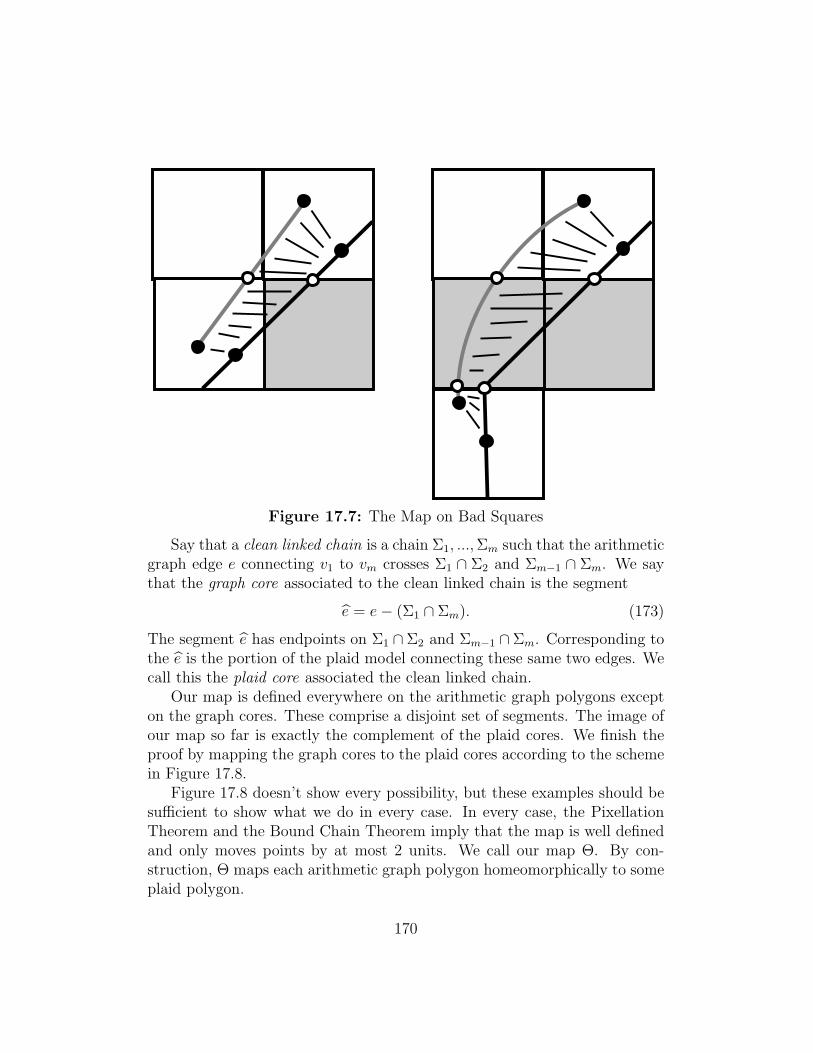
Figure 17.7: The Map on Bad Squares

Say that a clean linked chain is a chain Σ1, ...,Σm such that the arithmeticgraph edge e connecting v1 to vm crosses Σ1 ∩ Σ2 and Σm−1 ∩ Σm. We saythat the graph core associated to the clean linked chain is the segment

e = e− (Σ1 ∩ Σm). (173)

The segment e has endpoints on Σ1 ∩Σ2 and Σm−1 ∩Σm. Corresponding tothe e is the portion of the plaid model connecting these same two edges. Wecall this the plaid core associated the clean linked chain.

Our map is defined everywhere on the arithmetic graph polygons excepton the graph cores. These comprise a disjoint set of segments. The image ofour map so far is exactly the complement of the plaid cores. We finish theproof by mapping the graph cores to the plaid cores according to the schemein Figure 17.8.

Figure 17.8 doesn’t show every possibility, but these examples should besufficient to show what we do in every case. In every case, the PixellationTheorem and the Bound Chain Theorem imply that the map is well definedand only moves points by at most 2 units. We call our map Θ. By con-struction, Θ maps each arithmetic graph polygon homeomorphically to someplaid polygon.

170

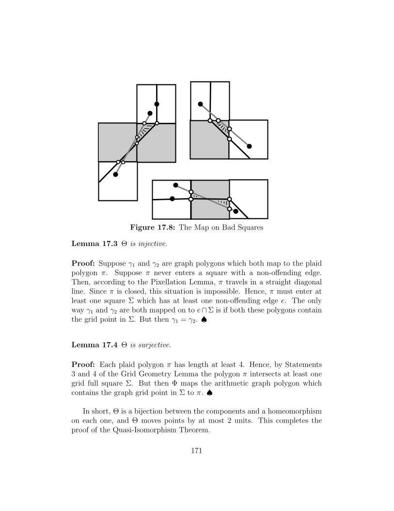
Figure 17.8: The Map on Bad Squares

Lemma 17.3 Θ is injective.

Proof: Suppose γ1 and γ2 are graph polygons which both map to the plaidpolygon π. Suppose π never enters a square with a non-offending edge.Then, according to the Pixellation Lemma, π travels in a straight diagonalline. Since π is closed, this situation is impossible. Hence, π must enter atleast one square Σ which has at least one non-offending edge e. The onlyway γ1 and γ2 are both mapped on to e∩Σ is if both these polygons containthe grid point in Σ. But then γ1 = γ2. ♠

Lemma 17.4 Θ is surjective.

Proof: Each plaid polygon π has length at least 4. Hence, by Statements3 and 4 of the Grid Geometry Lemma the polygon π intersects at least onegrid full square Σ. But then Φ maps the arithmetic graph polygon whichcontains the graph grid point in Σ to π. ♠

In short, Θ is a bijection between the components and a homeomorphismon each one, and Θ moves points by at most 2 units. This completes theproof of the Quasi-Isomorphism Theorem.

171

18 Proof of the Bound Chain Lemma

18.1 Length Two Chains

Let Σ1,Σ2 be a linked chain of length 2. This means that both Σ1 and Σ2

are plaid nontrivial and grid full, and a single plaid polygon runs throughboth. By the Pixellation Theorem, Σ1 and Σ2 are graph full as well.

a

1 2

v1

Figure 18.1: Σ1 and Σ2, and an uncaught offending edge.

Let vj be the graph grid point in Σj. Suppose that no graph edge incidentto v1 crosses Σ1 ∩ Σ2. Then there must be an offending edge a incident tov1 and associated to Σ1 ∩ Σ2. This edge must cross either the bottom orthe top of Σ1, and we have shown it crossing the bottom. But the picturecontradicts Statement 5 of the Pixellation Theorem, because the catch for awould involve Σ2, and Σ2 would be grid empty in the catch.

The argument in the preceding paragraph shows that there is some graphedge e1 incident to v1 which crosses Σ1 ∩ Σ2. Likewise, there is some graphedge e2 incident to v2 ∈ Σ2 which crosses Σ1 ∩ Σ2. If e1 and e2 are disjoint,then we have a bad configuration. The Bad Configuration Lemma rules thisout. Since the arithmetic graph is embedded, one of our two edges connectsv1 to v2, and in fact these two edges must coincide. (Otherwise we contradictthe Pixellation Theorem.) In short, Σ1,Σ2 is a bound chain.

172

18.2 Length Three Chains: Case A

Here we consider a length 3 chain in which the three squares are the samehorizontal row.

1 32

e1

e3v1

v3

Figure 18.2 A horizontal chain

Lemma 18.1 There is an edge of the arithmetic graph connecting v1 and v3.

Because the plaid polygon in Σ2 is not a diagonal segment, there is no wayto involve Σ2 in a catch for an offending edge incident to v1 and associatedto Σ1 ∩Σ2. Hence, Σ1 ∩Σ2 is not an unused edge of Σ1. Hence there is somegraph edge e1 incident to v1 and crossing Σ1∩Σ2. The same argument showsthat there is an arithmetic graph edge e3 associated to Σ3 which crossesΣ2 ∩ Σ3.

If the other endpoint e1 of e1 lies in Σ3 then this other endpoint mustbe v3, because there is at most one graph grid point in Σ3. So, to finishthe proof, we just have to rule out the other possible squares which couldpotentially contain the endpoint of e1.

The edge e1 has length less than 2 because ‖dT‖2 <√2 and e1 is the

image of a vector in Z2 of length at most√2. This bound on the length cuts

down on the possibilities where e1 could end up. For one thing, e1 cannot endup in any square to the right of Σ3. Also, e1 cannot cross the line one unitabove the top of Σ2, by Statement 3 of the Pixellation Theorem: no errantedges. EHence, the other endpoint of e1 lies in the row of squares above Σ2.We will consider the 3 cases when e1 ends in a square in the row above Σ3.The “below” case has the same treatment.

173

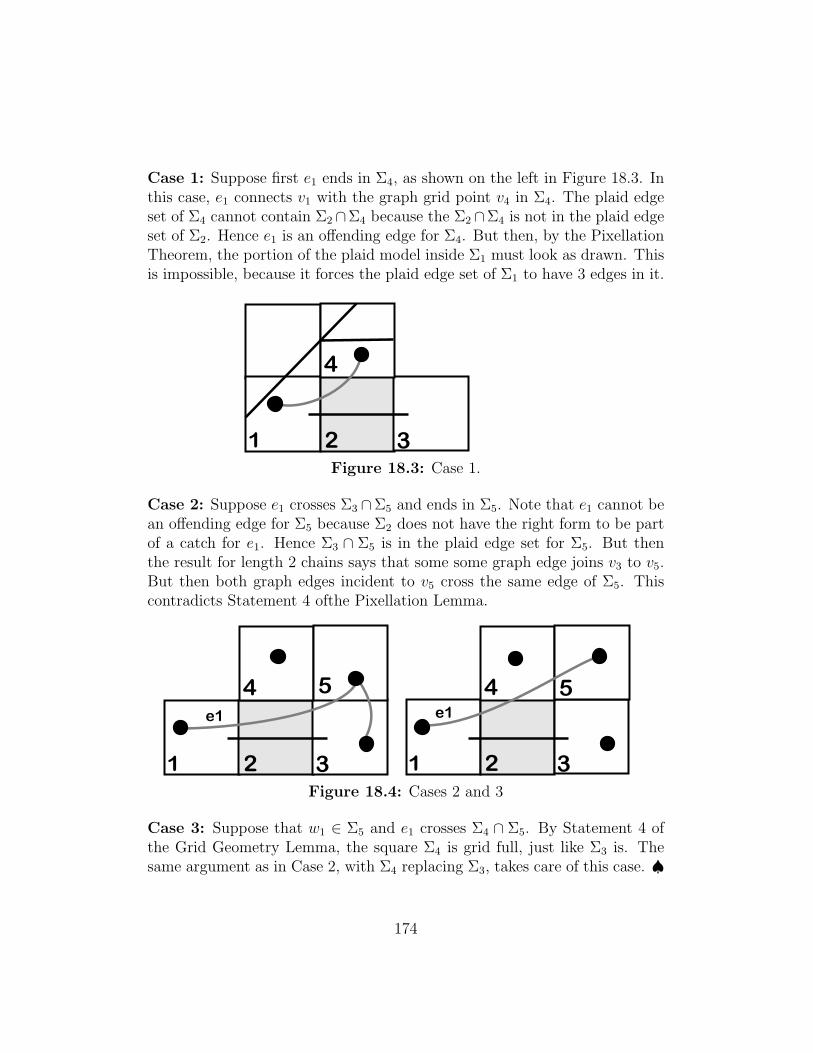
Case 1: Suppose first e1 ends in Σ4, as shown on the left in Figure 18.3. Inthis case, e1 connects v1 with the graph grid point v4 in Σ4. The plaid edgeset of Σ4 cannot contain Σ2∩Σ4 because the Σ2∩Σ4 is not in the plaid edgeset of Σ2. Hence e1 is an offending edge for Σ4. But then, by the PixellationTheorem, the portion of the plaid model inside Σ1 must look as drawn. Thisis impossible, because it forces the plaid edge set of Σ1 to have 3 edges in it.

1 32

4

Figure 18.3: Case 1.

Case 2: Suppose e1 crosses Σ3 ∩Σ5 and ends in Σ5. Note that e1 cannot bean offending edge for Σ5 because Σ2 does not have the right form to be partof a catch for e1. Hence Σ3 ∩ Σ5 is in the plaid edge set for Σ5. But thenthe result for length 2 chains says that some some graph edge joins v3 to v5.But then both graph edges incident to v5 cross the same edge of Σ5. Thiscontradicts Statement 4 ofthe Pixellation Lemma.

1 32

54

e1

1 32

54

e1

Figure 18.4: Cases 2 and 3

Case 3: Suppose that w1 ∈ Σ5 and e1 crosses Σ4 ∩ Σ5. By Statement 4 ofthe Grid Geometry Lemma, the square Σ4 is grid full, just like Σ3 is. Thesame argument as in Case 2, with Σ4 replacing Σ3, takes care of this case. ♠

174

18.3 Length Three Chains: Case B

Here we consider a length 3 chain in which the three squares are the samevertical column. Our proof refers to Figure 18.5

This situation is not quite the same as in Case A because we can have2 horizontally consecutive grid empty squares. If neither Σ4 nor Σ5, shownin Figure 18.5, is grid empty, then the same argument as in Case A applieshere. We just have to worry about the case when one of Σ4 or Σ5 is gridempty. We will consider the case when Σ5 is grid empty. The other case hasthe same treatment.

54

1

2

e1

e3

v3

v1

v6

6

Figure 18.5: A vertical chain

In order to avoid finishing the proof as in Lemma 18.1 both edges e1 ande3 must cross Σ2 ∩Σ5. Neither edge can end in Σ5 because Σ5 is grid empty.If e1 crosses the bottom edge of Σ5 then e1 blocks e3 from exiting Σ5, whichis a contradiction. Hence e1 does not exit the bottom edge of Σ5. Similarly,e3 cannot cross the top edge of Σ5. Hence, both e1 and e3 cross Σ5 ∩ Σ6.But then e1 and e3 are errant edges, and this contradicts Statement 3 of thePixellation Theorem.

175

18.4 Length Three Chains: Case C

Now we consider the remaining kind of length 3 chain, shown in Figure 18.6.As usual, let vj be the graph grid point in Σj for j = 1, 3. We want to provethat an arithmetic graph edge connects v1 to v3. This case is rather painful.

v3

2 1

v1

3

e3

e1

Figure 18.6

By Statement 5 of the Pixellation Theorm, Σ1 ∩Σ2 cannot be an unusededge with respect to Σ1, for the following reasons.

• If the associated offending edge were to cross through the top of Σ1,then the plaid segment in Σ2 (which is part of the catch) would havethe wrong position.

• If the associated offending edge were to cross through the bottom ofΣ1, then the plaid segment in Σ3 (which is part of the catch) wouldhave the wrong position.

Hence some graph edge e1 incident to v1 crosses Σ1 ∩ Σ2. The same ar-gument applies to Σ3. So, we can assume that the edges e1 and e3 are as inFigure 18.6. We will show that e1 has its other endpoint in Σ3. Since thereis only one graph grid point in Σ3, the other endpoint of e1 must be v3. Inshort, e1 is the desired arithmetic graph edge connecting v1 and v3. Thereare 6 situations we must rule out, and we deal with them in turn.

176

Case 1: Suppose e1 ends in Σ4. Since Σ2 ∩ Σ4 is not in the edge set ofΣ4, the edge e1 is offending with respect to Σ4. Given the negative slope ofe1, the associated unused edge must be the right edge of Σ4 and the catchmust involve Σ1,Σ2,Σ4. But then the plaid segment in Σ1 is in the wrongposition. This is a contradiction. The long Y -shaped graph in Figure 18.7shows the shape of the plaid arc implied by the existence of the catch, andthis contradicts the fact that the plaid arc in Σ1 also crosses into Σ2.

2 1

v1

3

e1

4v4

2 1

v1

3

e1

5 4

v5

v4

Figure 18.7: Cases 1 and 2

Case 2: Suppose e1 ends in Σ5 and that e1 crosses Σ4∩Σ5. By Statement4 of the Grid Geometry Lemma, the square Σ4 is grid full. So, Σ4 and Σ5

are both grid full. If e1 is an offending edge with respect to Σ5, then theassociated unused edge is the bottom edge of Σ5. But then the catch for e1must involve Σ2,Σ4,Σ5, and the plaid segment in Σ2 is in the wrong position.Hence Σ4∩Σ5 is in the edge set for Σ5. Hence Σ4,Σ5 form a linked chain andsome arithmetic graph edge joins v4 and v5. This contradicts the Statement4 of the Pixellation Theorem.

177

Case 3: Suppose that e1 ends in Σ5 and crosses Σ5 ∩ Σ6, as shown on theleft in Figure 18.8. If Σ6 is not grid empty, then the same argument in Case2 finishes the job. So, we may assume that Σ6 is grid empty.

Now, e1 cannot be an offending edge with respect to Σ5 for the samereason as in Case 2. Thus, Σ5 ∩ Σ6 is in the plaid edge set for Σ6. Theleft edge of Σ6 cannot be in the plaid edge set for Σ6 because this wouldmake e1 an errant edge for Σ5. Hence, the segment of the plaid model in Σ6

connects Σ5 ∩ Σ6 to Σ6 ∩ Σ7. But then, by Case B in the previous section,some arithmetic graph edge connects Σ5 to Σ7, as shown in Figure 18.10.But then two arithmetic graph edges cross Σ5 ∩Σ6, contradicting Statement4 of the Pixellation Theorem.

2 1

v1

3

e1

7

2 1

v1

3

e1

6

5

e3

v6

v5

Figure 18.8: Cases 3 and 4

Case 4: Suppose that e1 ends in Σ6 and e3 crosses Σ2 ∩Σ6. If e3 ends at v6,then both e1 and e3 cross the same edge of Σ6 and we contradict Statement4 of the Pixellation Theorem. Since e3 has length less than 2 and is not anerrant edge for Σ3, the only possibility is that e3 ends at v5. But the sameargument as in Case 3 shows that e3 is not an offending edge for Σ5. HenceΣ6,Σ5 is a linked chain. But then some other edge of the arithmetic graphconnects v6 to v5. This contradicts Statement 4 of the Pixellation Theorem.

178

Case 5: Suppose that e1 ends in Σ6 and e3 does not cross Σ6 ∩ Σ2. Notethat e1 blocks e3 from crossing the top of Σ2, so e2 crosses Σ1 ∩ Σ2.

Note that e1 is an offending edge for Σ6, because Σ2 does not have Σ6∩Σ1

in its plaid edge set. The plaid segment in Σ2 is not in the correct positionfor Σ2 to be part of a catch for e1, as would happen if e1 had negative slope.Hence e1 has positive slope. Note that e3 also has positive slope, because itrises up to cross Σ3 ∩ Σ2. So, both e1 and e2 have the same slope. (In thereflected case, both would have negative slope.)

There are two kinds of distingished edges having positive slope, and onlyone of them has a horizontal projection of length greater than 1. (The samegoes in the negative slope case, which arises in the reflected case.) We knowthat the horizontal projection of e1 is greater than 1. If the horizontal pro-jection of e3 is greater than 1, then e1 and e3 must be parallel. However, thenwe contradict Statement 6 of the Grid Geometry Lemma. We have foundtwo parallel distinguished lines which intersect the same vertical edge of asquare. In short e3 has horizontal projection at most 1. Hence the endpointof e3 is either in Σ1 or in Σ7.

If the endpoint of e3 lies in Σ1, we are done. So, consider the case whenthe endpoint of e3 lies in Σ7, as shown in Figure 18.9. In this case, we getthe same contradiction as in Case 4.

2 1

v1

3

e1

6

e3

v6

Figure 18.9: Case 5

179

Case 6: Suppose that w1 ∈ Σ8 or w1 ∈ Σ9. Then e1 has positive slope andhorizontal projection at least 1. If e3 does not cross Σ2 ∩Σ6 then we get thesame contradiction as in Case 5. So, we can assume that e3 crosses Σ2 ∩Σ6,as shown in Figure 18.10. But then, as Figure 18.10 indicates, e3 cannot bean offending edge for Σ6 because the plaid segment in Σ3 is not in the rightposition. Hence, Σ2 ∩ Σ6 is in the edge set for Σ6. But this would make theedge set of Σ2 have 3 members, which is a contradiction.

2 1

v1

3

e1

6

8

e3

9

Figure 18.10: Case 6

This completes the analysis of Case C. At this point we have proved theBound Chain Lemma for all linked chains, except those of length 4.

180

18.5 Length Four Chains: Case A

Suppose that Σ1,Σ2,Σ3,Σ4 is a length 4 linked chain, and all four of thesesquares are on the same row. The same argument as in Case 3A above

shows that there must be some graph edge e1, incident to v1, which crossesΣ1∩Σ2. Figure 18.11 shows a tree of possibilities. We will show that, actually,this case cannot occur. Without loss of generality, we will consider the casewhen e1 does not end up in a row of squares below our chain. Since e1 haslength less than 2, and e1 is not an errant edge, e1 must end either in Σ5 orΣ6.

1 32

65

e1

v1

v6

v5

4

Figure 18.11: Four-in-a-row case

Case 1: Suppose e1 lands in Σ5. Since Σ2 ∩ Σ5 is an unused edge for Σ5

and e1 crosses this edge, e1 must be an offending edge associated to the leftedg of Σ5. But then Σ1,Σ2,Σ5 are part of the catch for this edge. The plaidsegment in Σ1 is in the wrong position for this.

Case 2: Suppose e1 lands in Σ6 and crosses Σ5 ∩Σ6. Then e1 cannot be anoffending edge for Σ6 because the plaid segment in Σ3 is in the wrong posi-tion for it to participate in the required catch. Hence, some other arithmeticgraph edge joins v5 and v6. But then two graph edges are incident to v6 andcross Σ5 ∩ Σ6. This contradicts Statement 4 of the Pixellation Theorem.

Case 3: Suppose e1 lands in Σ6 and crosses Σ3 ∩ Σ6. The same kind ofargument as in Case 1 works here.

181

18.6 Length Four Chains: Case B

Suppose that Σ1,Σ2,Σ3,Σ4 is a length 4 linked chain, and exactly 3 of thesesquares are on the same row. Without loss of generality, we consider the caseshown in Figure 18.12. The same argument as in Case A above shows thatthere must be some graph edge e1, incident to v1, which crosses Σ1 ∩ Σ2.

Since e1 has length less than 2 and cannot be an errant edge, e1 must endin one of the squares Σ4,Σ5,Σ6,Σ7. Moreover, all these squares are grid full,by Statement 4 of the Grid Geometry Lemma. We want to show that e1 endsin Σ4. There are 4 cases to rule out. All 4 cases are handled by argumentsjust like those in Cases 4A1 and 4A2 above.

1 32

45

76

e1

v1

v7

v6

v5

v4

Figure 18.12: Three-in-a-row case.

Remark: We have stopped short of ruling out the existence of chains likethis, but we think that they never actually occur.

182

18.7 Length Four Chains: Case C

Suppose that Σ1,Σ2,Σ3,Σ4 is a length 4 linked chain, making a 2× 2 blockas shown in Figure 18.13.

The same argument as in previous cases shows that there is some graphedge e1 incident to v1 which crosses Σ1∩Σ2. We want to show that e1 connectsv1 to v4. Actually, this situation is impossible, given that we already knowthat e1 crosses Σ1 ∩ Σ2. So, our argument will really show that this kind oflinked chain is impossible.

Before we start our analysis, we make special mention of the squares Σ6

and Σ9. We do not know in general whether thess squares are grid full or gridempty. However, these squares are irrelevant for all our arguments unless e1actually ends in them. In those cases, the relevant square is grid full, bydefinition. So, in all relevant cases, Σ6 and Σ9 are grid full, as drawn.

5 32

4

87

e1

v1

v5

v4

6 8 9

10

Figure 18.13: Block case

Case 1: Suppose e1 ends in Σ5 or Σ10. This is the same as Case 4A1.

Case 2: Suppose e1 lands in Σ6, Σ8, or Σ9. In all these cases, the argu-ment is the same as in Case 4A2.

183

Case 3: Suppose that e1 lands in Σ7. Here we redraw the picture to fo-cus more particularly on this case. Since Σ7 ∩ Σ2 is not in the edge set forΣ2, the edge e1 must be an offending edge in Σ7 associated to Σ7 ∩ Σ2.

If e1 has negative slope, then Σ2,Σ5,Σ6,Σ7 form the catch for e1. Butthe catch must be of the first kind, and e1 must connect v7 to v5. This is acontradiction. If e1 has positive slope, then a similar argument shows thatactually e1 connects v7 to v4, another contradiction.

5 32

41

7

v4

6

Figure 18.14: Case 3

18.8 Length Four Chains: Case D

There is only one remaining case, and this case actually occurs. Supposethat Σ1,Σ2,Σ3,Σ4 is a length 4 linked chain, making a zig-zag pattern as inFigure 18.15 below.

As in Case 3C, it could happen that the edge Σ1 ∩ Σ2 is an unused sidefor Σ1. In this case, there is an offending edge e associated to Σ1 ∩ Σ2. Thecatch for e must be of the second kind because Σ3 is grid empty. The catchinvolves Σ1,Σ2,Σ3,Σ4,Σ10, and by definition e must end in Σ4 as desired. So,we just have to worry about the case when some graph edge e1 is incidenctto v1 and crosses Σ1 ∩ Σ2.

184

5 32

101

7

e1

v1v10

6 4 8

9

v4 v8

v9

Figure 18.15: zig-zag case

The same reasons as in Case 4C rule out the possibility that e1 ends in Σ5,Σ6, or Σ7. We just have to rule out e1 ending in Σ8 or Σ9. The same remarksas in Case 4C apply to the drawing of the square Σ8: This square could beeither grid full or grid empty, but in the case relative to the argument it isgrid full.

Case 1: Suppose e1 ends in Σ8 and crosses Σ4 ∩ Σ8. The argument in Case4B2 rules this out: Two graph edges would be incident to Σ8 and would crossΣ4 ∩ Σ8.

Case 2: Suppose e1 ends in Σ8 and crosses Σ9 ∩ Σ8. If e1 is not an of-fending edge for Σ8 then we get the same contradiction as in Case 1. But ife1 is an offending edge for Σ8 then, inspecting the nature of the catches, wesee that e1 must connect v8 to v10.

Case 3: Suppose e1 ends in Σ9. Looking at the portion of the plaid segmentin Σ3, we see that Σ3 ∩ Σ9 is not in the plaid edge set for Σ9. Hence e1 isan offending edge for Σ9. The catch for e1 must be of the first kind, becauseΣ10 is grid full. But then e1 connects v9 to v10, a contradiction.

185

19 The Graph Reconstruction Formula

The purpose of this chapter is to present a formula which we call the Re-construction formula, which relates the geometry of the graph grid to thegraph PET classifying map. Combining this formula with the Graph MasterPicture Theorem, we will prove Statement 1 of the Pixellation Theorem.

19.1 Main Result

Recall that X = R3× [0, 1]. For each parameter A, the affine group acting on

X in connection with the graph PET acts as an abelian group of translations.Precisely, this group is Λ(Z3), where

Λ =

1 0 0−1 1 + A 0−1 1− A 1 + A

Z3 (174)

Given a point ξ ∈ G, let [ξ] ∈ R2/Z2 denote the equivalence class of ξ.We now explain how we can use the map Φ to determine [ξ].

We introduce linear maps Θ1,Θ2 : R3 → R:

Θ1(x, y, z) = x, Θ2(x, y, z) =y − Ax1 + A

. (175)

Checking on the obvious basis for Λ, we see that Θj(Λ) ⊂ Z. ThereforeΘ1 and Θ2 both give well defined maps from R3/Λ, the domain for the graphcompactification at A, to the torusR/Z. Hence, we have a locally affine map

Θ : R3/Λ→ R2/Z2, L = [(Θ1,Θ2)]. (176)

The goal of this section is to establish the following result.

Lemma 19.1 (Reconstruction)

[ξ] = Θ Φ(ξ). (177)

We call this equation the Reconstruction Formula. Equation 177 allows usto get control over how the arithmetic graph sits with respect to Z2. We’vealready proven that no point of G lies on the boundary of an integer unitsquare. So, we can interpret both sides of Equation 177 as referring to pointsin the open integer unit square (0, 1)2. We fix a parameter A throughout theproof.

186

Lemma 19.2 Equation 177 holds at ξ = T (0, 0).

Proof: A direct calculation shows that

[ξ] =( 1

2q,

q − p2q(q + p)

).

Next, we compute

Φ(ξ) =( 1

2q,1

2q,1

2q, A

).

A direct calculation then shows that

Θ2(Φ(ξ)) =(p/q)(1/2q)− (1/2q)

1 + (p/q)=

q − p2q(q + p)

.

Hence, the two sides of the equation agree. ♠

Lemma 19.3 If Equation 177 holds at ξ, it also holds at ξ ± dT (0, 1).

Proof: We do the (+) case. The (−) case has the same proof. Let ξ′ =ξ + dT (0, 1) = ξ + (1,−P ). Here P = 2A/(1 + A). We compute

Θ Φ(ξ′)−Θ Ψ(ξ) = Θ(1, 1, 1) =(1,

1− A1 + A

)= (1,−P + 1).

The last expression is congruent to ζ ′ − ζ = (1,−P ) mod Z2. ♠

Lemma 19.4 If Equation 177 holds at ξ, it also holds at ξ ± dT (1, 1).

Proof: We do the (+) case. The (−) case has the same proof. We havedT (1, 1) = (1 + A, 1 + A). Using the same notation as in the previousargument, we have

Θ Φ(ξ′)−Θ Ψ(ξ) = Θ(1 + A, 1 + A, 1 + A) = (1 + A, 1− A) = ζ ′ − ζ.

This completes the proof ♠

These three lemmas together show that Equation 177 holds on all ofdT (Z2), as desired.

187

19.2 Eliminating Most Double Crossings

In this section we eliminate most of the double crossings mentioned in §17.3.This section does not use either the Reconstruction Formula or the GraphMaster Picture Theorem.

Let T be the canonical affine transform. See §12.3. Recall that a distin-guished edge is an edge having vertices v1, v2 ∈ T (Z) such that v1−v2 = T (ζ),where ζ is one of the 8 shortest nonzero vectors in Z2. We say that the edgebelongs to the family F(i, j) is ζ = ±(i, j).

A double crossing is a configuration of the kind shown in Figure 19.1below. The configuration consists of two adjacent unit integer squares Σ1

and Σ2, graph grid points v1 ∈ Σ1 and v2 ∈ Σ2, and disjoint distinguishededges e1 and e2 incident to v1 and v2 respectively which both cross Σ1 ∩ Σ2.

Lemma 19.5 A bad configuration must have the following structure.

• Σ1 ∩ Σ2 is horizontal.

• The edge connecting v1 to v2 belongs F(1, 0).

• At least one of the two edges e1 or e2 belongs to F(−1, 1).

Proof: Let f = v2 − v1. By Statement 5 of the Grid Geometry Lemma, fmust be a distinsuighed edge.

We define S1 to be the set of 8 distinguished edges incident to v1. Wethink of these edges as vectors pointing out of v1. This set has a naturalcyclic order on it. Likewise we define S2.

Let Σ12 = Σ1∩Σ2. The edges of S1 which intersect Σ12 closest to f ∩Σ12

are obtained by turning f one click in S1, either clockwise or counterclock-wise. Likewise, the edges of S2 which intersect Σ12 closest to f ∩ Σ12 areobtained by turning (−f) one click in S2, counter clockwise or counterclock-wise. The two turnings must be in the same direction, because otherwise theresulting edges would intersect.

So, the shortest possible distance between the two intersection points oc-curs when e1 and e2 are parallel. Statement 6 of the Grid Geometry Lemmanow says that Σ12 is horizontal and the parallel lines are of type (−1, 1).Looking at the proof of Statement 6 of the Grid Geometry Theorem given in§12.4, we see that this forced f ∈ F(1, 0). ♠

188

19.3 Eliminating the last Double Crossing

Now we will use the Reconstruction Formula and the Graph Master PictureTheorem to rule out the last kind of double crossing. This proves Statement1 of the Pixellation Lemma. We will suppose that the arithmetic graph has adouble crossing for some parameter A and derive a contradiction. The readeris warned in advance that our proof, at the end, is just a computer assistedcalculation.

We will consider the case when the edge e1 shown on the left side ofFigure 19.1 is in the family F(−1, 1). The other case, when e2 ∈ F(−1, 1),has a similar proof. Indeed, the second case follows from the first case andfrom the rotational symmetry of the arithmetic graph.

v1e2

e1 v2

1

2

AFigure 19.1: A double crossing.

Let G denote the graph grid and let Φ : G→ X be the graph classifyingmap.

189

Lemma 19.6 Φ(v1) lies in the region of X ∩ H, where H is the half spacegiven by the equation x < 1− A.

We know that the edge joining v1 to v2 is in the family F(1, 0). The firstcoordinate of T (1, 0) is A, so the horizontal distance from v1 to v2 is A. Thatmeans that v1 is within 1 − A units of the left edge of Σ1, as shown on theright half of Figure 19.1.

By the Reconstruction Formula, Φ(v1) lies in the region

RA = XA ∩ x| x < 1− A. (178)

RA lies in the regionH ∩ X, (179)

where H is the halfspace given by the equation x < 1−A. Recall that the co-ordinates on this space are (x, y, z, A), so H is an defined by inteer equations.Also, H is invariant under the action of the graph lattice Λ defined in §13.1. ♠

Recall that we parametrize X ⊂ R4 with coordinates (x, y, z, A). So, His a halfspace defined by integer equations. Moreover, H is invariant underthe action of the graph lattice defined in §13.1.

The way the graph classifying map works is that we look at Φ(v1) andrecord the labels of the polytope in each partition which contains this point.

Lemma 19.7 Assuming that a bad configuration exists, one of the polytopesin one of the partitions has the label (1,−1) and intersects H.

Proof: There are two polytopes of interest to us: the one in each parti-tion which contains Φ(v1). These polytopes both intersect H. One of thesepolytopes is responsible for the assignment of the vector e1 to v1. Call thisthe magic polytope. The magic polytope Since e1 is in the family F(−1, 1),the label of the magic polytope is either (−1, 1) or (1,−1). We check thatT (1,−1) is the one with positive y coordinate. Hence, the label of the magicpolytope is (1,−1). ♠

Now for the computer assisted part of the proof. We check that no poly-tope at all in the (+) partition has the label (1,−1), and the only polytopesin the (−) partition intersect H. This is obvious from the pictures on mycomputer program, and I will describe in the last chapter the short linearalgebra computation which checks it. This completes the proof.

190

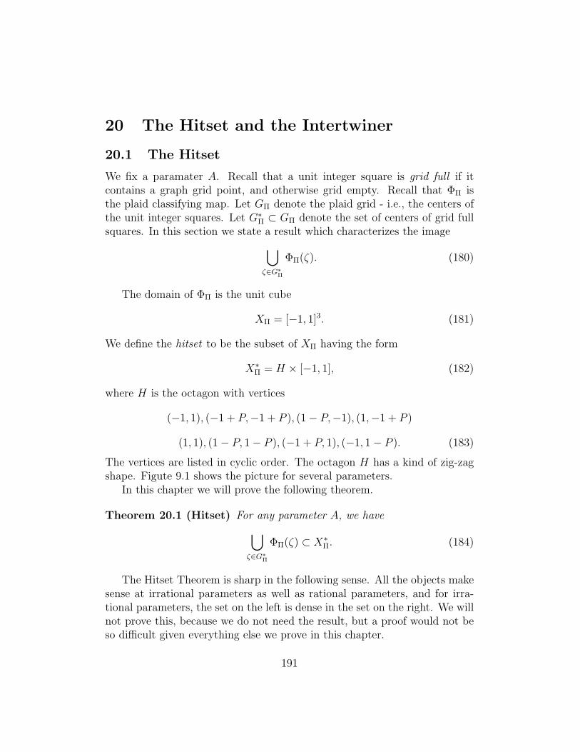
20 The Hitset and the Intertwiner

20.1 The Hitset

We fix a paramater A. Recall that a unit integer square is grid full if itcontains a graph grid point, and otherwise grid empty. Recall that ΦΠ isthe plaid classifying map. Let GΠ denote the plaid grid - i.e., the centers ofthe unit integer squares. Let G∗Π ⊂ GΠ denote the set of centers of grid fullsquares. In this section we state a result which characterizes the image

⋃

ζ∈G∗

Π

ΦΠ(ζ). (180)

The domain of ΦΠ is the unit cube

XΠ = [−1, 1]3. (181)

We define the hitset to be the subset of XΠ having the form

X∗Π = H × [−1, 1], (182)

where H is the octagon with vertices

(−1, 1), (−1 + P,−1 + P ), (1− P,−1), (1,−1 + P )

(1, 1), (1− P, 1− P ), (−1 + P, 1), (−1, 1− P ). (183)

The vertices are listed in cyclic order. The octagon H has a kind of zig-zagshape. Figute 9.1 shows the picture for several parameters.

In this chapter we will prove the following theorem.

Theorem 20.1 (Hitset) For any parameter A, we have

⋃

ζ∈G∗

Π

ΦΠ(ζ) ⊂ X∗Π. (184)

The Hitset Theorem is sharp in the following sense. All the objects makesense at irrational parameters as well as rational parameters, and for irra-tional parameters, the set on the left is dense in the set on the right. We willnot prove this, because we do not need the result, but a proof would not beso difficult given everything else we prove in this chapter.

191

In Figure 20.1 below we show the polygon H for the parameters k/5 fork = 1, 2, 3, 4. (The picture makes sense for all parameters, and not just evenrational ones.) Actually, we show not just H but also the image of H underthe action of the lattice ΛΠ. We think of this lattice as acting on the xyplane just by forgetting about the third coordinate. The lattice is generatedby the vectors (2, P ) and (0, 2).

Thanks to the product structure of XΠ and X∗Π, the planar pictures weshow capture all the information. The various images of H fit together toform infinite bands which look like zigzags. As A → 0 the zigzags cometogether and fill up the plane.

Figure 20.1: The orbit ΛΠ(H) for parameters A = k/5, k = 1, 2, 3, 4.

192

20.2 The Projective Intertwiner

The symbol Ψ will denote the map which we call the projective intertwiner .We will define Ψ after we specify its domain and range. Recall that our totalspace is X = R3 × [0, 1].

Domain: The domain of Ψ is XΠ, though our theorem really only concernsthe image of Ψ on the hitset X∗Π. The set XΠ is the fundamental domain for

the lattice Λ1 acting on X. See §7.1.We write

XΠ = XΠ,− ∪XΠ,+, (185)

Where XΠ,+ consists of those points (x, y, z, P ) where x ≤ y and XΠ,− cn-sists of those points there y ≤ x. This is a partition of XΠ into two isometrichalves.

Range: The range of Ψ isXΓ = X/Λ, (186)

where Λ is the graph lattice defined in §13.1.

The Map: Now we define the map

Ψ : XΠ → XΓ.

For (x, y, z, P ) ∈ XΠ,±, we define

Ψ(x, y, z, P ) =

[1

2− P(x− y,−y − 1, z + P + 1, P

)± (1, 0, 0, 0)

]

Λ

(187)

That is, we add or subtract 1 depending on which half of the partition ourpoint lies in, and we take the result mod Λ. In the next section we checkthat Ψ is well defined even in boundary cases. The map Ψ is a piecewisedefined integral projective transformation. If we hold P fixed and restrictΨ to a slice, then Ψ is an affine transformation. We call Ψ the projectiveintertwiner .

The Main Result: Let GΓ denote the graph grid. Let GΠ denote theplaid grid. Each point ζΓ ∈ GΓ lies in the interior of a unique integer square.We let ζΠ ∈ GΠ denote the center of this square.

193

Let ΦΠ : GΠ → X1 denote the plaid classifying map. Recall that, atthe parameter A, the range of ΦΠ is contained in the slice R3 × P, whereP = 2A/(1 + A). Let ΦΓ : GΓ → X/Λ be the graph classifying map.

Theorem 20.2 (Intertwining) The following holds for every even rationalparamater:

ΦΓ(ζΓ) = Ψ ΦΠ(ζΠ) ∀ζΓ ∈ GΓ. (188)

Remarks:(i) I checked Equation 188 computationally for all relevant points and allparameter p/q with q < 30. This check is not meant as a substitute for arigorous proof, but it is nice to know. I didn’t check the Hitset Theorem assystematically, but my computer program plots the left and right hand sidesof Equation 184, and one can see that it always works.(ii) Notice in Equation 187 that the fourth coordinate on the right hand sideis A, because A = P/(2−P ). Thus, Ψ maps the relevant slices to each other.(iii) It might be nicer if there were a global projective transformation from

X to itself which works in place of our piecewise projective map Ψ. However,we have Ψ(TX(V )− V ) = (2, 0, 0, 0). The vector on the right does not havefor them λ(W ) −W for any transformation λ ∈ Λ1, the plaid lattice. Thissituation makes the existence of a global projective intertwiner impossible.On the other hand, below in §20.8 we will modify the domain of Ψ so thatΨ is projective throughout the interior of the new domain. When we look atthe action of Ψ on the new domain, we will see the canonical nature of Ψ.See Lemma 20.4 for instance.(iv) When it comes time to prove the Pixellation Theorem, we shall be in-terested in the action of Ψ on the polytopes of the plaid triple partition. Atfirst, it looks like we might have trouble, due to the piecewise nature of Ψ.However, it turns out that every plaid triple polytope is contained in one ofthe two pieces of the partition of XΠ.(v) Our proof will show that a suitable formulation of the Intertwining The-orem holds for all parameters, and not just even rational ones. Indeed, itbasically follows from continuity.(vi) The reader who is keen to see how the proof of the Pixellation Theoremworks might want to take the Hitset Theorem and the Intertwining Theo-rem for granted on the first reading. Our proof of the Pixellation Theoremonly uses the truth of these statements, and not any theory developed duringtheir proof. §21.3 gives a good illustration of how we use the IntertwiningTheorem.

194

20.3 Well Definedness

Since Ψ is only piecewise defined, we have to worry about the cases whenthere are two competing definitions for Ψ. In our discussion of this matter,the symbol (∗) stands for a coordinate value that we don’t care about. Wefix some even rational parameter for the discussion.

There are three issues. One issue is that perhaps

ΦΠ(ζ) = (−1, ∗, ∗).

In this case, the two points

φ+ = ΦΠ(ζ), φ− = ΦΠ(ζ) + (2, P, P )

are equally good representatives. Here φ± ∈ XΠ,±. An easy calculation showsthat

Ψ(φ−)−Ψ(φ+) =1

2− P(2− P,−P, PP,−P, 2− P

)− (2, 0, 0) =

(−1,−A,A) ∈ Λ1. (189)

Hence, either representative gives rise to the same point in the range.The second issue seems more serious, in view of Remark (v) above. It

might happen thatφ = ΦΠ(ζ) = (v, v, ∗).

That is, φ lies on the boundary of both pieces of the partition of XΠ. Let’scheck that this situation cannot arise for the images of points of GΠ. Suchpoints have the form (x, y) where x and y are half integers. We compute that

ΦΠ(x, y) = (2Px+ 2y, 2Px, ∗) + (2m,Pm, ∗), (190)

for a suitable integer m. We also observe that 2y is odd. Equation 190 leadsto

P =2m+ 2y

m.

This is impossible, because P = 2p/(p+ q), and 2m+ 2y is an odd integer.The third issue is that ΦΠ(ζ) = (∗, u, v) with either u = ±1 or v = ±1

or both. The case u = ±1 is impossible for similar reasons that we have justdiscussed. When v = ±1 it has replacing v by v ∓ 2 has no effect on theIntertwining formula.

195

20.4 Strategy of the Proof

The rest of the chapter is devoted to proving the Hitset Theorem and theIntertwining Theorem. We prove these two results at the same time becausethey are closely related to each other. Here are the steps of the proof. Wefix a parameter A = p/q.

• We prove the Intertwining Theorem for points of the form

ζn = (n+ 1/2)(1 + A, 1− A), n = 0, 1, 2, .... (191)

These points all belong to GΓ because ζ0 is the anchor point and ζn −ζ0 = ndT (1, 1). Here T is the canonical affine transformation. We callthe points in Equation 191 the diagonal points .

• We prove the Hitset Theorem for the points in Equation 191.

• We prove the following induction step: Suppose that the Hitset The-orem is true for some graph grid point ζ. Then it is also true forζ + dT (0, 1). We call this Hitset Induction.

• We prove the following induction step: Suppose that the IntertwiningTheorem is true for some graph grid point ζ. Then it is also true forζ + dT (0, 1). We call this Intertwiner Induction.

Let L denote the lattice of symmetries generated by the vectors (ω2, 0)and (0, ω). Here ω = p + q, as usual. We have already shown that both theplaid model and the arithmetic graph are invariant under L. We say that anL-orbit is an orbit of L acting on the graph grid. By symmetry, it suffices toprove our two theorems on a set which contains at least one point of everyL-orbit

The four steps above combine to to prove that the two theorems holdtrue on sets of the form dT (B) where B is a ball in Zn of arbitrarily largeradius. For sufficiently large B, the set dT (B) intersects every L orbit.

Remark: It would have been nice if the set of points ζn intersected everyL-orbit. If this was true, we would not need the induction part of the proof.Likewise, it would have been nice if, starting from a single point (such as theanchor), we could reach every L-orbit just by repeatedly adding dT (0, 1).If this was true, we would not need the first two steps of our proof. Alas,neither of these step-saving situations is true.

196

20.5 The Intertwining Theorem on the Diagonal

In this section we prove the Intertwining Theorem for points of the form

ζn =(n+

1

2

)(1 + A, 1− A), n = 0, 1, 2, ... (192)

These points all belong to GΓ, because ζn = ζ0+dT (n, n) and ζ0 is the anchorpoint.

We fix the value of n. It is convenient to consider the sub-intervals

Rn,k =( 2k

2n+ 1,2k + 1

2n+ 1

), k = 0, ..., (n− 1). (193)

Ln,k =(2k − 1

2n+ 1,

2k

2n+ 1

), k = 1, ..., (n− 1). (194)

We ignore the endpoints of these intervals; the boundary cases, when relevant,follow from continuity.

Let I = (A0, A1) be one of the intervals of interest. We will sometimesuse the following trick to bound certain numerical quantities that depend onA ∈ I. When the quantity is monotone, we get the bounds by evaluatingthe expression on the boundary values A = A0 and A = A1. We call thismethod the boundary trick .

When A ∈ Ln,k (respectively R ∈ Ln,k, the point ζn lies in the left(respectively right) half of the square with center

ζn,k =(n+

1

2, n+

1

2

)+ (k,−k). (195)

First we consider the case when A ∈ Ln,k. We have

ΦΠ(ζn,k) ≡ (P (2n+2k+1)+(2n−2k+1), P (2n+2k+1), 2P (2n+1)). (196)

The symbol ≡ means that we still need to reduce mod Λ1 to get a vector inthe fundamental domain.

The boundary trick tells us that the first coordinate in Equation 196 liesin (

1 + 2k + 2n− 1 + 2n

k + n, 1 + 2k + 2n

)(197)

So, we subtract off the lattice vector (n+ k)(2, P, P ). This gives

ΦΠ(ζn,k) ≡ (P (2n+ 2k + 1)− 4k + 1, P (1 + k + n), 2P (2− k + 3n)). (198)

197

The boundary trick tells us that the second coordinate in Equation 198 liesin the interval (−1, 1)+2k. Subtracting (0, 2k, 0) from Equation 198, we geta point in the fundamental domain:

ΦΠ(ζn,k) = (P (2n+2k+1)−4k+1, P (1+k+n)−2k, P (2−k+3n)+2β). (199)

Here β is some integer whose value we don’t care about.The interval check shows that the first coordinate in Equation 199 is

larger than the second coordinate. (We apply the trick to the difference ofthe coordinates.) Hence the point in Equation 199 lies in XΠ,−. We also have

ΦΓ(ζ) ≡(n+

1

2

)(1 + A, 1 + A, 1 + A) mod Λ. (200)

Here Λ is the graph lattice. (In all these equations we are leaving off thefourth coordinate; we know this works out already.)

A calculation, which we do in Mathematica, shows that

Ψ(ΦΠ(ζn,k)− ΦΓ(ζ) =(−1− k − n)(1,−1,−1)+

(−2− 2n)(0, 1 + A, 1− A)+(1− k + β)(0, 0, 1 + A).

In other words, we have written the difference between the quantities asan integer combination of vectors in the graph lattice Λ. Hence, the twoquantities are equal, as desired.

When A ∈ Rn,k the calculation is very similar and we will just describethe differences. This time the interval trick tells us to subtract off the vector(n + k + 1)(2, P, P ) from the point in Equation 196. Then, as in the othercase, we subtract off (0,−2k, 0). The result is

ΦΠ(ζn,k) = (P (2k+2n+1)−4k−1, P (k+n)−2k, P (1−k+3n)+β) (201)

The interval trick shows that this point lies in XΠ,+. Now we compute

Ψ(ΦΠ(ζn,k)− ΦΓ(ζ) =(−k − n)(1,−1,−1)+

(−1− 2n)(0, 1 + A, 1− A)+(1− k + β)(0, 0, 1 + A).

This gives us the same desired conclusion as in the first case.

198

20.6 The Hitset Theorem on the Diagonal

Now we prove the Hitset Theorem for the points we considered in Step 1.We first consider the case when A ∈ Ln,k. The triangle ∆L with vertices

(−1 + P,−1 + P ), (1,−1 + P ), (1, 1) (202)

is the convex hull of 3 of the vertices and is contained in the polygon definingthe hitset.

LR

Figure 20.2: The triangles ∆L and ∆R.

Let ξ denote the point in the plane obtained by taking the first twocoordinates of the point in Equation 199. That is:

ξ = (P (2n+ 2k + 1)− 4k + 1, P (1 + k + n)− 2k). (203)

It suffices to prove that ξ ∈ ∆L for all A ∈ Ln,k. One of the sides of ∆L

is the line x = 1, and certainly ξ does not cross this line; it corresponds toone of the sides of the fundamental domain. Another side of ∆L is the liney = −1 + P . The interval trick shows that ξ stays above this line. Finally,the other side of ∆L is the line y = x. We already know that ΦΠ(ζ) ∈ XΠ,−,and this is the equivalent to the statement that ξ lies to the right of this line.These three conditions together imply that ξ ∈ ∆L. My computer programallows you to see a plot of ξ and ∆L for all the relevant parameters.

Now consider the case when A ∈ Rn,k. This time we use the triangle∆R = −∆L, obtained by negating all the coordinates of the vertices of ∆.This time we want to show that the point

(P (2k + 2n+ 1)− 4k − 1, P (k + n)− 2k) (204)

lies in ∆R. The same arguments as aboe shows that this point lies to theright of the line x = −1, below the line y = 1− P , and to the left of the liney = x. This does the job for us.

199

20.7 Hitset Induction

Here we will prove Hitset Induction modulo what we call the geometric claim.We will prove the geometric claim at the end of the chapter.

We set ζΓ = ζ and ζ ′Γ = ζ+dT (0, 1). Similarly, we define ζΠ and ζ ′Π. HereζΠ is the center of the unit integer square that contains ζΓ. Since we will bementioning both the plaid lattice and the graph lattice, we let ΛΠ denote theplaid lattice and ΛΓ denote the graph lattice.

We havedT (0, 1) = (1,−P ). (205)

From this equation, we see that we have one of two possibilities for ζΠ′ − ζΠ.This difference either equals (1, 0) or (1,−1). To be more precise, let Ghi

Γ

denote the union of those choices of ζΓ = (x, y) such that x − floor(x) > P .Define ζ loΠ to be the complementary set. For even rational parameters, itnever happens that y = floor(y) = P , because then ζ ′Γ would be lie on theboundary of a unit integer square.

Let H lo denote the parallelogram with vertices

(1−3P, 1−3P ), (1−P, 1−P ), (−1+P, 1) (−1−P, 1−2P ). (206)

Let Hhi denote the polygon with vertices

(−1+P,−1+P ), (1−P,−1), (3−3P, 1−2P ) (1−P, 1−P ). (207)

These polygons are not subsets of H. However, the orbits ΛΠ(Hhi) and

ΛΠ(Hlo) together give a partition of ΛΠ(H). The dark region is the lo orbit

and the light region is the hi orbit .

Figure 20.4: The orbits ΛΠHlo and ΛΠH

hi for A = 1/4 and A = 3/4.

200

Geometric Claim:

• ζΓ ∈ GhiΓ implies ΦΠ(ζΠ) ∈ ΛΠ(H

hi × [−1, 1])

• ζΓ ∈ GloΓ implies ΦΠ(ζΠ) ∈ ΛΠ(H

lo × [−1, 1])We call this claim the geometric claim.

We introduce the new sets

(Hhi)′ = Hhi + (2P, 2P ), (H lo)′ = H lo + (2P − 2, 2P − 2). (208)

If ζΓ ∈ GhiΓ and the geometric claim is true, then

ΦΠ(ζ′Π) ∈ ΛΠ((H

hi)′ × [−1, 1]).

The same goes when we replace hi with lo. In the low case, we are using thefact that (2P − 2, 2P − 2) and (2P − 2, 2P ) are equal up to a vector in ΛΠ.

Now for the punchline. ΛΠ((Hlo)′) and ΛΠ((H

hi)′) give a second partitionof ΛΠ(H). Figure 20.5 shows the picture for the parameters A = 1/4 andA = 3/4.

Figure 20.5: The orbits ΛΠ(Hlo)′ and ΛΠ(H

hi)′ for A = 1/4 and A = 3/4.

We get exactly the same picture as in Figure 20.4 except that the pieces haveeach been translated.

What we are really saying is that there is an infinite polygon exchangetransformation on ΛΠ(H) which corresponds to the operation of adding thevector dT (0, 1) in GΓ. The orbit ΛΠ(H) decomposes into a countable unionof parallelograms, each partitioned into a light parallelogram and a dark one.Our map simply exchanges the light and dark pieces within each component.On each component, our map is essentially a rotation of a flat torus.

201

Figure 20.6 shows the two partitions side by side, for the parameter A =1/4. The “components” we are talking about are parallelograms which arebounded on opposite sides by lines of slope 1. For later reference, we callthese parallelograms dipoles . So, again, each dipole is partitioned into a lightand dark parallelogram, and our polygon exchange simply exchanges the twopieces within each dipole.

Figure 20.6: The two partitions of ΛΠ(H) for the parameter A = 1/4.

The Geometric Claim immediately implies Hitset Induction. Hence, theGeometric Claim implies the Hitset Theorem.

20.8 Changing the Fundamental Domain

Observe that the orbit ΛΠ(H) is simply a union of dipoles. Rather thanconsider XΠ = [−1, 1]3 as our fundamental domain for the action of ΛΠ, weinstead consider the fundamental domain to be

Υ× [−1, 1] (209)

where Υ is the dipole that intersects [−1, 1]2 to the right of the diagonal liney = x. Figure 20.7 shows Υ and how it sits with respect to [−1, 1].

202

Figure 20.7: The fundamental dipole.

We get an easier calculation if we use Υ × [−1, 1] as the domain for theprojective intertwiner Ψ. To do this, we need to define Ψ on the whole fun-damental domain, and check that the new definition agrees with the originalin the appropriate sense.

The points of Υ − [−1, 1]2 all lie to the right of [−1, 1]2, and one simplysubtracts off (−2,−P ) to get them back into [−1, 1]2. For any

φ ∈(Υ− [−1, 1]2

)× [−1, 1], (210)

We define Ψ(φ) using the branch of Φ which is defined for XΠ,−. Letφ∗ = φ− (2, P, P ) ∈ XΠ,+. Using the fact that φ ∈ XΠ,− and φ∗ ∈ XΠ,+, wecompute

Ψ(φ)−Ψ(φ∗) = (−1,−A,A) = (−1, 1, 1)− (0, 1 + A, 1− A) ∈ ΛΓ. (211)

So, our redefinition does not change anything. We can prove Induction State-ment 2 using the new fundamental domain. Moreover, the restriction of Ψto the new domain is projective throughout.

203

20.9 Intertwiner Induction

Since ΦΓ(x, y) = (x, x, x) mod ΛΓ, we have

ΦΓ(ζ′Γ)− ΦΓ(ζΓ) = (1, 1, 1) mod ΛΓ. (212)

Letφ = ΦΠ(ζΠ), φ′ = ΦΠ(ζ

′Π). (213)

To establish Intertwiner Induction, we just have to prove

Ψ(φ′)−Ψ(φ)− (1, 1, 1) ∈ ΛΓ. (214)

Using our new fundamental domain, and also the action of the map ΦΠ, wehave one of

φ− φ′ = (2P, 2P, 2P + 2β), φ′ − φ = (2P − 2, 2P − 2, 2β), (215)

depending on whether we are in the hi case or the lo case. Here β is someinteger whose value does not effect the calculation.

Hi Case:Ψ(φ′)−Ψ(φ)− (1, 1, 1) =

1

2− P(0,−2P, 2P + 2β

)− (1, 1, 1) =

(−1,−2A− 1, 2A− 1 + 2β(1 + A)) =

2β(0, 0, 1 + A) + (−1, 1, 1) + 2(0, A+ 1, A− 1) ∈ ΛΓ.

Notice that β plays no role at all in the final answer. To simplify the secondcalculation, we assume that β = 0.

Lo Case:Ψ(φ′)−Ψ(φ)− (1, 1, 1) =

1

2− P(0,−2P + 2, 0

)− (1, 1, 1) =

(−1,−A,−1) = (−1, 1, 1)− (0, 1 + A, 1− A)− (0, 0, 1 + A) ∈ ΛΓ.

This is what we wanted to prove.At this point, we have reduced the Intertwining Theorem and the Hitset

Theorem to the Geometric Claim.

204

20.10 Proof of the Geometric Claim

We will combine the Intertwining Formula with the Graph ReconstructionFormula. We are allowed to do this for the pair (ζΓ, ζΠ) by induction.

We introduce coordinates

ζΓ = (a, b), ΦΠ(ζΠ) = (x, y, z, P )

. Let [t] = t− floor(t).

Lemma 20.3

[a] =

[x− y2− P

], [b] =

[−2− P + P 2 + Px+ 2y − 2Py

2P − 4

]. (216)

Proof: DefineΨ ΦΠ(ζΠ) = (x∗, y∗, z∗, A).

For convenience, we repeat Equation 187 here:

Ψ(x, y, z, P ) =

[1

2− P(x− y,−y − 1, z + P + 1, P

)− (1, 0, 0, 0)

]

Λ

(217)

We always take the (−) option in Equation 187 because we are using thedomain Υ × [−1, 1] described in §20.8. The graph reconstruction formulatells us that

[a] = [x∗], [b] =

[y∗ − Ax∗1 + A

].

Combining this formula with Equation 217 and doing some algebra, we getEquation 216. ♠

The next result says that the formulas in Equation 216, which look messy,are actually as nice as possible.

Lemma 20.4 Equation 216 induces an affine diffeomorphism from Υ to[0, 1]2.

Proof: Forgetting about the brackets, the corresponding map on the planeis an affine diffeomorphism Ω. The first coordinate of Ω is obviously constantalong lines of slope 1. These lines are parallel to the diagonal sides of Υ. We

205

claim that the second coordinate of Ω is constant along lines parallel to theother two sides of Υ. To see this, we plug in the equation

y =( −P2− P

)x+ c. (218)

and observe that the resulting expression

f(c) =2 + P − P 2

4− 2P+(P − 1

2− P)c (219)

is independent of x.The left and right sides of Υ are given by the equations y = x and

y = x− (2− P ). Hence Ω maps the left and right sides of Υ respectively tothe left and right sides of the integer unit square [0, 1]2. The bottom and topsides of Υ are given by taking

c0 =P − 2

2, c1 =

P − 2

2+

1− P2− P (220)

in Equation 218. We check that f(c0) = 1 and f(c1) = 0. Hence Ω maps thetop and bottom of Υ respectively to the bottom and top of [0, 1]2. ♠

The Geometric Claim follows immediately from the analysis in the pre-vious lemma. It says that

ΛΓ(Hhi)∩Υ = Ω−1([0, 1]×[P, 1]), ΛΓ(H

lo)∩Υ = Ω−1([0, 1]×[0, P ]). (221)

In light of Equation 216, this last equation is equivalent to the GeometricClaim.

This completes the proof of the Geometric Claim, and thereby completesthe proof of both the Hitset Theorem and the Intertwining Theorem.

206

21 Correspondence of Polytopes

In this chapter we prove Statement 2 of the Pixellation Theorem modulosome integer linear algebra calculations. We also set up the kind of problemwe need to solve in order to prove Statements 3,4, and 5 of the PixellationTheorem. We fix some parameter A that is in the background of the wholediscussion. Also, as in some previous chapters, we reserve the word squarefor unit integer squares.

21.1 The Triple Partition

Suppose that P1 and P2 are two partitions of X into polytopes, say

Pk =⋃

i

Pi,k. (222)

We define the common refinement to be

P1#P2 =⋃

i,j

Pi,1 ∩ Pj,2. (223)

This is the usual definition. In case the polytopes in the two partitions haverational vertices, the polytopes, in the common refinement will also haverational vertices. This construction may be iterated, so that we can take then-fold common refinement of n partitions.

Let P0 be the partition of X that we have described above. We define

Pk = F k(P0). (224)

In other words, we take the original partition and apply a power of the PETdynamics. We define the triple partition to be the common refinement

T P = P−1#P0#P1. (225)

We will prove that every vertex of every polytope in T P has a coordinateswhich are divisors of 60. That is, if Q is a polytope of T P , then 60Q is aninteger polytope.

Each polytope in T P has a 6 letter label. We simply concatenate thelabels for each of the 3 polytopes involved in the intersection, starting withthe label for the polytope in P−1 and ending with the label for the polytope

207

in P1. This 6 letter label has the following meaning. We look at the labelof the polytope containing ΦA(c) and the label determines the shape of thelength 3 arc of the oriented plaid component that is centered at c. Figure21.1 illustrates this principle with two examples. In Figure 21.1 we show thelabel and the corresponding path. We hope that these examples suffice toconvey the general idea.

EWEWEW

Figure 21.1: The meaning of the 6 letter labels

We define the reduced triple partition to be partition

RT P = T P#([−1, 1]3 × [0, 1]). (226)

Essentially we are taking the pieces of T P which lie inside our favorite funda-mental domain for Λ1, but in case any of the pieces slop over the boundary ofthis fundamental domain, we chop them off. Once again, for everyQ ∈ RT P ,the scaled polytope 60Q is integral.

We think of the polytopes in RT P as being labeled by the same 6-letterlabels, modulo reversal of the labeling. With this interpretation, we caninterpret that map ΦAG→ X as a classifying map for unoriented arcs of theplaid model having combinatorial length 3. We just use the action of Λ1 tomove ΦA(c) into RT P and then we read off the label.

There is one minor issue that we need to address. It follows from The-orem 7.5 that ΦA(c) always lies in the interior of a polytope of T P , but itmight happen that there are several images of ΦA(c) on the boundary of thefundamental domain. This is the usual problem with fundamental domains.However, in this situation, all the images will lie in polyopes having the samelabels. So, even when there is some ambiguity in interpreting ΦA as a mapfrom G into RT P , the ambiguity is harmless.

208

Even though it is somewhat less natural than T P , we will use RT Pfor the proof of the Quasi-Isomorphism Theorem because it makes certainformulas simpler.

21.2 Proof of Statement 2

Statement 2 of the Pixellation Theorem says that a grid full square is plaidtrivial if and only if it is graph trivial.

The reduced triple partition RT P consists of 218 polytopes in the fun-damental domain XΠ = [−1, 1]3. We call these polytopes Π0, ...,Π217.

Lemma 21.1 Suppose that Σ is a grid full square. If Σ is plaid trivial thenΣ is graph trivial.

Proof: In our listing, there are 6 polytopes in RT P having null labels,namely Π0, ...,Π5. We observe that Ψ(Πj) is contained in a single polytope

Γj = Γj,+ = Γj,−

in the graph partition, and that Γj is null labeled. (This is why Γj,+ = Γj,−.)Suppose that Σ is a grid full plaid trivial square for some parameter. Let

ζΠ be the center of Σ. Let ζΓ be the graph grid point in GΓ which is containedin Σ.

By the Plaid Master Picture Theorem,

ΦΠ(ζΠ) ⊂5⋃

j=0

Πj.

By the Intertwining Theorem,

ΦΓ(ζΓ) ⊂5⋃

j=0

Ψ(Πj) ⊂5⋃

j=0

Γj.

By the Graph Master Picture Theorem, the portion of the arithmetic graphassociated to ζΓ is trivial. That is, Σ is graph trivial. ♠

Lemma 21.2 Suppose that Σ is a grid full square. If Σ is graph trivial thenΣ is plaid trivial.

209

Proof: We will prove the contrapositive: If Σ is plaid nontrivial then Σ isgraph nontrivial. We observe that each of the polytopes Π6, ...,Π217 has anontrivial label. We also observe the following:

• Ψ(Πj) is contained in a single graph polytope Γj,+ and a single graphpolytope Γj,− for j = 6, ..., 179. The labels of these graph polytopesare all nontrivial

• Ψ(Πj) is contained in a single graph polytope Γj,− and a union of twograph polytope Γj,+,0 and Γj,+,1 for j = 180, ..., 198. The labels of thesegraph polytopes are all nontrivial.

• Ψ(Πj) is contained in a single graph polytope Γj,+ and a union of twograph polytope Γj,−,0 and Γj,−,1 for j = 199, ..., 217. The labels of thesegraph polytopes are all nontrivial.

Combining the information listed above with the Plaid Master PictureTheorem, the Graph Master Picture Theorem, and the Intertwining Theo-rem in the same way as the previous proof, we get the conclusion of thislemma. ♠

21.3 A Sample Result

Let us press the method of the previous section a bit harder, in order to seeboth its power and its limitations. Figure 21.2 shows a particular arc of theplaid model. Depending on the way the triple is oriented, it corresponds totiles in RT P labeled NEWEWS or SWEWEN.

Figure 21.2: The triple of type NEWEWS or SWEWEN.

Lemma 21.3 (Sample) Every time the triple of the type shown in Figure21.2 appears in the arithmetic graph and the central square Σ is grid full, thetwo edges incident to the grid graph vertex in Σ are in F(0, 1) and F(0,−1).

210

Proof: There are 6 polytopes in RT P having the relevant labels. The oneslabeled NEWEWS are listed as Π7,Π138,Π165. The ones labeled SWEWENare listed as Π103,Π130,Π159.

Recall that Ψ is the projective intertwining map. We check by directcomputation that, for each j ∈ 7, 103, 130, 138, 159, 165 there are polytopesΓj,+ and Γj,− in the (+) and (−) graph PET partitions respectively so that

Ψ(Πj) ⊂ Γj,+ ∩ Γj,−. (227)

When we inspect the labels of these graph polytopes we observe that

• The label of Γj,+ is always (0, 1).

• The label of Γj,i is always (0,−1).

Now let us put this information together. Suppose we see the triplefrom Figure 21.2 in the plaid model for some parameter A. The rest of thediscussion implicitly refers to the parameter A. Let ζΓ be the vertex of thegraph grid GΓ contained in the central square Σ of the triple. The sameargument as in the previous section shows that

ΦΓ(ζΓ) ∈⋃

j=7,103,130,138,159,165

Γj,+ ∩ Γj,−. (228)

But then, by the Master Picture Theorem, the two edges incident to ζΓ arein F(0, 1) and F(0,−1). ♠

10.2 shows us the kind of conclusion we can draw from Lemma 21.3.

10.2: Some possible conclusions from Lemma 21.3.

Lemma 21.3 tells us that every time we see the triple in Figure 21.2, wesee the arithmetic graph edges shown in (in grey) in 10.2. However, it mighthappen that one of these grey edges crosses the top or the bottom of thecentral square rather than the sides, as it the Pixellation Theorem suggests.

211

Lemma 21.3 tells us the local geometry of the arithmetic graph but not how itcrosses the edges of the central square. So eliminate the second option shownin 10.2 (as well as other bad options, we need to study how our machineryalso determines the edge crossings.

In the rest of this chapter, we set up conventions and notation for thekind of problem we need to solve.

21.4 Fixing Orientations

Recall that there are both oriented and unoriented versions of the Plaid andGraph Master Picture Theorems. We have stated the Intertwining Theoremfor the unoriented versions, because the proof is simpler. However, this forcesus to deal with orientations in a somewhat ad hoc way.

As we mentioned above, there are 218 polytopes in RTP. Each of thesepolytopes has a 6 letter label which specifies an oriented arc of combinatoriallength 3 in the plaid model. The catch is that we are using the small domainX/Λ1 as the image of the plaid classifying map ΦΠ, rather than the double

cover X/Λ2.Thus, if ζΠ ∈ GΠ is some point, the label of the polytope inRT P contain-

ing ΦΠ(ζΠ) might specify the opposite orientation on the plaid arc through

ζΠ. More precisely, the assigned orientation is correct if and only if ΦΠ(ζΠ)

is congruent mod Λ2 to a point in the fundamental domain XΠ. Here ΦΠ isthe lift of Π to the double cover X/Λ2. At the same time, in order to figureout the orientations on the graph polygons, we would need to look at the liftΦΓ of the graph classifying map ΦΓ.

Getting these orientations right is a tedious business, and we have adifferent way of dealing with it. We ignore the “true” orientations comingfrom the lifted maps and we simply make a guess as to how the plaid arcscorrespond to the graph arcs. For example, in 10.2, it is pretty clear thatthe grey edge pointing left should be associated to the left half of the plaidtriple.

Now we explain the convention in more detail, by way of example. Figure21.3 shows an enhanced version of 21.2, specifically for Π7. Again, the labelof Π7 is NEWEWS, and this determines the orientation.

212

Figure 21.3: The case of Π7: a correspondence of type 1

We observe experimentally that the (−) partition assigns the label (0,−1),and this corresponds to the leftward pointing edge. Likewise, the (+) parti-tion assigns the label (0, 1), and this corresponds to the rightward pointingedge. Thus, we associate the (−) partition with the tail end of the triple andthe (+) partition with the head end. For this reason, we call Π7 type 1 . Wewould call Πj type 0 if, according to our experimental observations, the (+)edge is associated with the tail and the (−) edge is associated with the tail.

We guess the type for each of the 218 polytopes in the plaid triple par-tition, and these types are stored in the computer program. In most cases,as for Π7, the picture is completely obvious, and in a few cases, like the oneshown in 10.2 for Π49 the picture is not quite as obvious but still pretty clear.

Figure 21.4: The case of Π48: a correspondence of type 0.

Logically, it does not matter how we arrived at these guesses, or whetherthey agree with the true answer which can be cleaned by looking at the lifts.The point is simply that the proof runs to completion with the guesses made.In hindsight, our guesses surely agree with the true answer, but we do notneed to prove this and we will not.

213

21.5 Edge Crossing Problems

To each index i = 6, ..., 218 we associate what we call an edge crossing prob-lem. We will first give the general definition and then we will work out theexample of Π7.

Given Πk, there corresponds a triple of squares Σ−1,Σ1,Σ1 and an ori-ented plaid arc running through it, as in Figures 21.3 and 21.4. We label thesquares so that Σ1 is the head square in the type 1 case and the tail squarein the type 0 case. In other words, the arithmetic graph edge associated tothe (±) partition should point generally from Σ0 to Σ± for both types.

There are two kinds of edge crossing problems associated to Pk. Onekind is labeled (k,+, i, j, L). Here L ∈ N,S,E,W is an edge of Σ0 thatthe arithmetic graph edge dT (i, j) associated to the (+) partition could po-tentially cross (as in the right hand side of Figure 21.3) but according to thePixellation Theorem is not supposed to cross. These crossing problems reallyonly depend on the pair (Σ,Σ+). The other kind of edge crossing problemis labeled (k,−, , i, j, L), and has a similar explanation with (−) in place of(+).

Let’s consider the case of P7. The two crossing problems are (7,+, 0, 1, N)and (7,−, 0,−1, S). The other two possibilities, namely (7,+, 0, 1, E) and(7,−, 0,−1,W ), are the ones predicted by the Pixellation Theorem. Theyare not problems at all, but rather goals .

We have already mentioned that the first 6 of the plaid triple polytopescorrespond to the trivial grid full squares. There are another 174 polytopes,labeled Π6, ...,Π179, which have the property that there are unique graphpolyropes Γk,+ and Γk,− such that

Ψ(Πk) ⊂ Γk,±. (229)

Each of these contributes 2 edge crossing problems, giving a total of 348.The 19 polytopes Π180, ...,Π198 are such that

Ψ(Πk) ⊂ Γk,+,0 ∪ Γk,+,1, Ψ(Πk) ⊂ Γk,−. (230)

That is, Ψ(Πk) is contained in a union of two graph polytopes from the (+)partition and 1 from the (−) partition. In this case, there are two possiblelocal picture of the arithmetic graph associated to this plaid triple. This doesnot bother us, as long as the edge crossings come out right. Each of these 19polytopes contributes 3 edge crossing problems. This gives us another 57.

214

The 19 polytopes Π199, ...,Π217 are such that

Ψ(Πk) ⊂ Γk,−,0 ∪ Γk,−,1, Ψ(Πk) ⊂ Γk,+. (231)

Each of these 19 polytopes contributes 3 edge crossing problems, giving yetanother 57 crossing problems.

The grand total is 462 edge crossing problems. In the next chapter wewill introduce the machinery needed to solve all these problems, so to speak.A solution amounts to a proof that the given case does not actually occur.Actually, we will be able to solve 416 of the problems. The remaining 46, inthe cases where the pixellation really does fail, are involved in the catchesfor the offending edges discussed in the Pixellation Theorem. Once we havesolved all the problems we can solved, and classified the exceptions, the restof the Pixellation Theorem just comes down to inspecting the data generatedby the program.

215

22 Edge Crossings

22.1 The Graph Method

Here we explain the first method we use for solving the edge crossing prob-lems. We fix a parameter A throughout the discussion. Let GΓ denote thegrid graph. Let ζΓ ∈ G be some point, contained in a square Σ. As inprevious chapters, the word square always means a unit integer square.

We assume that ζΓ is a nontrivial vertex of the arithmetic graph. Lete be one of the edges of the arithmetic graph incident to ζΓ. We think ofe as a vector pointing from v out of Σ. From the Grid Geometry Lemma,we know that e crosses some edge of Σ. We say that e is of type (i, j, L) ife = dT (i, j) and L ∈ S,W,N,E is the label of the edge of Σ which e crosses.

Remark: We allow the possibility that e is of two types. This would hap-pen if e crosses Σ at a vertex. We think that this never actually happens,but we have not ruled it out. In any case, this eventuality does not bother us.

Let ΦΓ denote the graph classifying map. We define

(x, y, z, A) = ΦΓ(ζΓ) (232)

Lemma 22.1 (Graph Avoidance) The following is true.

1. If x ∈ (A, 1) then e is not of type (−1, 0,W ).

2. If x ∈ (0, A) then e is not of type (−1, 1,W ).

3. If y ∈ (A, 1) then e is not of type (0,−1, N).

4. If y ∈ (2A, 1 + A) then e is not of type (0, 1, S).

5. If x ∈ (1− A, 1) then e is not of type (1,−1, E).

6. If x ∈ (0, 1− A) then e is not of type (1, 0, E).

Proof: We will treat the first three cases. The last three cases follow fromsymmetry. More precisely, reflection in the center of the square [0, 1]2 carriesthe sets used to analyze Case N to the sets used to analyze Case 7-N. Figure22.1 illustrates our arguments.

216

Figure 22.1: The first three cases

Case 1: We have

dT (−1, 0) =(− A,−1 + 2A− A2

1 + A

).

This vector points southwest and has slope greater than 1. So, in order forthis edge to cross the west edge, it must lie in the triangle with vertices

(0, 0), (0, 1)( A2 + A

1 + 2A− A2

).

We call this triangle the danger zone. The line through this third point andparallel to e contains the vertex between the south and west edges. The darktriangles in Figure 22.1 are hand-drawn versions of the danger zones in eachcase.

The Graph Reconstruction Formula tells us that the conditions x ∈ (A, 1)correspond to the condition that the first coordinate of ξΓ lies in (A, 1). Theregion of possibilities is the lightly shaded region on the left hand side of fig-ure 23.1. As depicted in the figure, the two sets we have defined are disjoint.

Case 2: The argument is the same, except this time the danger zone hasvertices

(1, 0), (1, 1),( 4A

4A− A2

),

and the condition x ∈ (0, A) corresponds to these same conditions on thefirst coordinate of ξΓ. Again, the two sets are disjoint. This is shown in themiddle square of Figure 22.1.

Case 3: The argument is the same, except this time the danger zone hasvertices

(0, 1), (1, 1),(1,

1− A1 + A

).

217

and the condition y ∈ (A, 1) corresponds, via the Reconstruction Formula toξΓ lying in the interior of the parallelogram with vertices

(0,

A

1 + A

),

(0,

1

1 + A

),

(1,

1− A1 + A

),

(0, 0

).

Again, these sets are disjoint. This case is shown on the right side of Figure22.1. ♠

Remark: In the previous result, the cases (1, 1, N) and (−1,−1, S) aremissing. There is a similar result for these cases, but we will prove a resultbelow that is more powerful and subsumes these cases. So, we ignore themhere.

22.2 The Sample Result Revisited

In this section we explain how we solve the crossing problem (7,+, , 0, 1, S).In other words, we are trying to rule out the bad crossing indicated on theright hand side of Figure 21.2, which we repeat here with enhanced labeling.We really need to solve 6 crossing

Figure 22.2: The crossing problem (7,+, S).

The polytope Ψ(Π7) has 8 vertices:

• (60, 60, 0, 30)/60.

• (60, 40, 20, 20)/60.

• (40, 40, 0, 20)/60.

• (60, 40, 0, 20, )/60.

218

• (60, 60, 0, 20)/60.

• (45, 45, 0, 15)/60.

• (60, 45, 15, 15)/60.

• (60, 45, 0, 15)/60.

We have written the vertices this way so as to clear denominators. The factorof 60 works for every polytope in sight. (My program has a window whichallows the user to see the vertices of any polytope in any of the partitions.)

Recalling that we coordinatize X using the variables, note that

y ∈ [2A, 1 + 2A]. (233)

for all vertices of Ψ(Π7). By convexity, this equation holds for all points, andwe get strict inequality for points in the interior of Ψ(Π7).

It follows from the Master Picture Theorems and the Intertwining Theo-rem that

(x, y, z, A) = ΦΓ(ζΓ) ∈ interior(Ψ(Πy)). (234)

Hence y ∈ (2A, 1 + 2A). Case 4 of the Graph Avoidance Lemma, whichpertains to the triple (0, 1, S), solves this crossing problem.

The argument works the same way for all 6 crossing problems associatedto the bad crossing shown in Figure 22.2. It follows from symmetry (or froma similar argument) that the 6 crossings associated to the other arithmeticgraph edge in Figure 22.2 are also soluble. Thus, every time this patternoccurs in the plaid model for any parameter, and the central square is gridfull, the central square is pixellated.

Remark: Sometimes we use the Graph Avoidance Lemma in a differentway. To illustrate our other usage, we will solve the edge crossing problem(198,+,−1, 1, E). This time it turns out that the criterion in the GraphAvoidance Lemma for (1,−1, E) does not hold for Ψ(Π198). However, itdoes hold for Γ198,+,0, the relevant one of the two graph polytopes in the(+) graph partition whose union contains Ψ(Π198). So, again, we find thatΦΓ(ξΓ) cannot lie in the region corresponding to a situation where the graphedge incident to ζΓ crosses E.

For all the relevant crossing problems on which we use the Graph Avoid-ance Lemma, we will either apply the criteria to Ψ(Π) or to the relevantgraph polytope Γ. In short, we will use the one method or the other.

219

22.3 The Plaid Method

Here we discuss a second method for solving crossing problems. In the dis-cussion that follows, L ∈ N,S,E,W stands for one of the edge labels. To

10 of the 16 pairs (i, j, L). Let 〈i, j, L〉 denote the subset of X which assignsthe edge e = dT (i, j) to grid graph points ζΓ. in such a way that e crosses theedge L of the square containing the point ζΓ. The Graph Avoidance Lemmacan be interpreted as saying that certain regions in X avoid 〈i, j, L〉. Forinstance, the set x ∈ (A, 1) is disjoint from 〈−1, 0,W 〉.

Recall that X∗Π is the hitset. We are going to associate a polytopeZ(i, j, L) ⊂ XΠ such that one of two things is true:

• If P ∩ Z(i, j, L) = ∅ then Ψ(P ) ∩ 〈i, j, L〉 = ∅.

• If P ⊂ Z(i, j, L) then Ψ(P ∩X∗Π) ∩ 〈i, j, L〉 = ∅.

In the first case, we call P an excluder and in the second case we call P aconfiner . The other 6 pairs we simply ignore.

For each fixed parameter, our polytopes all have the form

Z(i, j, L) = Z ′(i, j, L)× [−1, 1], (235)

Where Z ′(i, j, L) is a polygon in the xy plane. We will list 4 of the 10 sets.The other 5 are obtained from the first 5 via the following symmetry.

Z(−i,−j, Lopp) = −Z(i, j, L). (236)

Here Lopp is defined to be the edge opposite L. For instance Eopp = W . Welist the 5 polygons Z ′(i, j, L) as a function of the parameter A, and recall thatP = 2A/(1 + A). The first set is an excluder and the other 5 are confiners.Here are the sets:

• Z ′(1, 1, N): (1− P, 1− P ), (P − 1, P − 1), (P − 1,−1), (1− P,−1).

• Z ′(1, 1, E): (1− P, 1− P ), (−1,−1), (1− P,−1).

• Z ′(0, 1, S): (−1,−1),(P − 1, P − 1), (1, P − 1), (1− P,−1).

• Z ′(1, 0, E) = Z ′(1, 1, E).

• Z ′(0,−1,W ) = Z ′(0, 1, S).

220

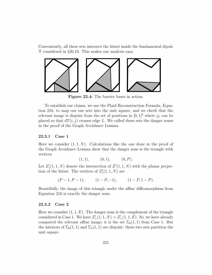
Conveniently, all these sets intersect the hitset inside the fundamental dipoleΥ considered in §20.10. This makes our analysis easy.

Figure 22.4: The barrier bases in action.

To establish our claims, we use the Plaid Reconstruction Formula, Equa-tion 216, to map our our sets into the unit square, and we check that therelevant image is disjoint from the set of positions in [0, 1]2 where ζΓ can beplaced so that dT (i, j) crosses edge L. We called these sets the danger zonesin the proof of the Graph Avoidance Lemma.

22.3.1 Case 1

Here we consider (1, 1, N). Calculations like the one done in the proof ofthe Graph Avoidance Lemma show that the danger zone is the triangle withvertices

(1, 1), (0, 1), (0, P ).

Let Z ′∗(1, 1, N) denote the intersection of Z ′(1, 1, N) with the planar projec-tion of the hitset. The vertices of Z ′∗(1, 1, N) are

(P − 1, P − 1), (1− P,−1), (1− P, 1− P ).

Beautifully, the image of this triangle under the affine diffeomorphism fromEquation 216 is exactly the danger zone.

22.3.2 Case 2

Here we consider (1, 1, E). The danger zone is the complement of the triangleconsidered in Case 1. We have Z ′+(1, 1, N) = Z ′+(1, 1, E). So, we have alreadycomputed the relevant affine image; it is the set Σ0(1, 1) from Case 1. Butthe interiors of Σ0(1, 1) and Σ1(1, 1) are disjoint: these two sets partition theunit square.

221

22.3.3 Case 3

Here we consider (0, 1, S). The danger zone is the same as the one in Case 4of the Graph Avoidance Lemma. It has vertices

(0, 0), (1, 0), (0, P ).

The set Z ′∗(0, 1, Z) is the triangle with vertices

(P − 1, P − 1), (1− P,−1), (1, P − 1).

The image of this set under the affine diffeomorphism is the triangle withvertices

(0, 1), (1, 1), (1, P ).

This triangle is clearly disjoint from the danger zone.

22.3.4 Case 4

Here we consider (1, 0, E). The danger zone has vertices

(1, 1), (1, 0),(1 + A− 2A2

1 + 2A− A2

)

We have Z ′(1, 0, E) = Z ′(1, 1, E). The analysis in Case 1 shows that theaffine image of Z ′+(1, 0, E) is the triangle with vertices

(1, 1), (0, 1), (0, P ).

The interior of this set is clearly disjoint from the danger zone.

22.3.5 Case 5

Here we consider (0,−1,W ). The danger zone has vertices

(0, 0), (1, 0), (1, P ).

We have Z ′(0,−1,W ) = Z ′(0, 1, S), the set from Case 3. As in Case 3, thevertices of the affine image of Z ′(0,−1,W ) is the triangle with vertices

(0, 1), (1, 1), (1, P ).

The interior of this set is disjoint from the danger zone.

222

22.4 Another Edge Crossing Problem

Here we solve another edge crossing problem, to illustrate the logic behind theuse of the Plaid Method. We use the notation from above. One of the crossingproblems is (50,+,−1,−1,W ). This time we find that Π50 ⊂ Z(−1,−1,W ).Therefore Hence

ΨΠ(ζΠ) ⊂ Z(−1,−1,W ). (237)

The existence of ζΓ means that the relevant square Σ is grid full.

ΨΠ(ζΠ) ⊂ Z(−1,−1,W ) ∩X∗Π. (238)

By the Intertwining Theorem

ΦΓ(ζΓ) ⊂ Ψ(Z(−1,−1,W ) ∩X∗Π). (239)

By the confining property of Z(−1,−1,W ),

ΦΓ(ζΓ) 6∈ 〈−1,−1,W 〉. (240)

This solves the crossing problem.

22.5 Out of Bounds

Sometimes none of the above methods works for a crossing problem, but thenwe notice that Πk lies entirely outside the hitset Z∗Π. In this case we call Πk

out of bounds . The corresponding crossing problem simply does not arise fora grid full square.

We will verify that Πk is out of bounds by showing that

Πk ⊂4⋃

i=1

Bi × [−1, 1]. (241)

Where B′1, B′2, B

′3, B

′4 are the following 4 triangles, described in terms of their

vertices:

1. B′1 : (−1,−1), (P − 1,−1), (P − 1, P − 1).

2. B′2 : (1− P,−1), (1,−1), (1, P − 1).

3. B′3 = −B′1.

223

4. B′4 = −B′2.

Figure 22.5 shows how these triangles sit in relation to the planar projectionof the hitset.

1

34

Figure 22.5: The out-of-bounds polygons in action.

Note that the union

Bi =⋃

P∈[0,1]

(B′i × P) (242)

is a convex polytope with integer coefficients. Here P = 2A/(1+A) as usual.This, showing that Πk ⊂ Bi for some pair (k, i) is just a matter of integerlinear algebra. We call the verification that Πk ⊂ Bi the out of bounds test .

224

23 Proof of the Pixellation Theorem

Pixellation Theorem. In this chapter, we prove Statements 3,4,5 of the Pixel-lation Theorem modulo certain integer computer calculations.

23.1 Solving Most of the Crossing Problems

Using the methods discussed in the last chapter, namely the Graph Method,the Plaid Method, and the Out of Bounds Test, we solve 416 of the 462crossing problems. Each case is like one of the ones considered in the previouschapter, but there are too many to do by hand. In the next chapter we willexplain the integer linear algebra tests we use to check each case.

There are 46 exceptional cases. Let’s call these 46 cases recalcitrant . Afew of the recalcitrant cases actually are soluble by more delicate methods -we would just need to look harder at the polytopes involved - but there isn’tany problem in our proof with leaving them unsolved.

23.2 Proof of Statement 3

Figure 17.3 shows examples of an errant edge when the two squares arestacked side by side. We repeat the picture here. We will consider thepicture on the right hand side of Figure 23.1 in detail. In this picture, thesquare with the dot is the central square and the top square is not part ofthe triple. So, we are only showing two of the three squares in the triple.

The codes associated to the figure on the right are either LLLEWS orSWELLL, depending on the orientation. Here L ∈ N,S,E,W is a labelwe don’t know. The corresponding errant edge must rise up at least 1 unit.This leaves dT (1,−1) and dT (1, 0) as the only possibilities.

1 2 1 2

Figure 23.1: errant edges

225

From the correspondence of polytopes explained in §21, we know thecomplete list of labels associated to relevant ends of the relevant triples. Wejust check, by a quick computer search (and also by inspection) that theerrant labels never arise. Thus, for instance, we never see the label (1, 0)associated to the head end of LLLEWS or the tail end of SWELLL. We ruleout the other possibilities similarly. Here is a list of the possible codes andthe forbidden labels. To save space, we only list half the possibilities. Theother half are obtained from these by 180 degree rotation. Also, of the halfwe do list, we only list the codes such that the corresponding errant edgewould be associated to the head of the triple. So, we would list LLLEWSonly in our example above. Here is the list.

• LLLEWS: (1, 0), (1,−1).

• LLLEWN: (−1, 0), (−1, 1).

• LLLEWE: (1, 0), (1,−1), (−1, 0), (−1, 1).

• LLLSNE: (−1,−1), (0,−1).

• LLLSNW: (1, 1), (0, 1).

• LLLSNS: (−1,−1), (1, 1), (0, 1), (0,−1).

We simply check that none of these bad situations actually arises. Therest of the proof of the Pixellation Theorem is devoted to proving Statements3 and 4. This takes more work.

23.3 Proof of Statement 4

Statement 4 of the Pixellation Theorem says that two arithmetic graph edgesincident to a vertex in a square never cross the same edge of that square. Thisresult follows immediately for the 416 cases in which can solve the crossingproblem: These cases are all pixellated and the edges in question cross thesame sides as the plaid model segments. It just remains to deal with the 46recalcitrant cases.

226

Figure 23.2: The recalcitrant cases

By direct inspection, we see that all of the recalcitrant cases are eitherpixellated or equivalent to the two cases shown in Figure 23.2. (By symmetry,we just have to inspect 23 of the 46 cases.) By equivalent we mean that thepicture is meant to be taken up to rotations and reflections.

Now consider the arithmetic graph edges associated to the a recalcitrantcase. The first edge, the one shown in Figure 23.2, is offending. The otheredge is either offending or not. If the other edge is not offending, then itmanifestly crosses a different edge of the central square. If the other edgeis offending, and crosses the same edge as the first offending edge, then thepicture must look like Figure 23.3.

Figure 23.3: A double edge crossing

There are exactly two cases like this, corresponding to P34 and P173. But,in both cases, we check that the polytope is involved in only one recalci-trant crossing problem. So, in these two cases, only one of the two edges isoffending.

This takes care of all the possibilities.

227

23.4 Proof of Statement 5

Each recalcitrant case corresponds to a plaid triple. Using the curve-followingdynamics discussed in in §7.5, we check which plaid triples could attach tothe one we have. We will illustrate what we mean by example and then statethe general result.

157 58

Figure 23.4: The triples corresponding to Π157 and Π58.

One of the recalcitrant triples is (157,−,−1, 0, S). The associated codefor Π157 is EWEWES. Figure 12.4 shows the situation. The offending edgegoes with the orientation of the plaid arc, and so we do the (+) dynamicsto figure out what happens to points in Π157. That is, we consider theimage F (Π157). (In the other case, when the offending edge goes against theorientation, we would use the map F−1.) We prove that

F (Π157) ⊂ Λ(Π58). (243)

Here Λ is the plaid lattice.We then check that Π58 is grid empty. This means that and unit integer

square in the plaid model classified by Π58 is grid empty. Here we mean thatΦΠ maps the center of the square into Π58. But then Equation 243 tells usthat the square on the right and side of any plaid triple associated to Π157 isgrid empty. We have shaded the trid empty squares.

Equation 243 says that every occurance of a plaid triple associated toΠ157 is conjoined, so speak, with the a plaid triple associated to Π58. Wehave also added in an extra square, even though we don’t know the picturein this square. Figure 12.5 shows the situation.

228

Figure 23.5: The plaid quadruple obtained by concatenating Π157 and Π38.

When we look at the curve following dynamics for the other recalcitrantcases, we discover that the same thing always happens: The side squareassociated to the offending edge is grid empty. Up to isometry, the picturealways looks like one of the cases of Figure 23.6.

Figure 23.6: Concatenations for the recalcitrant triples

The only thing we need to do in order to finish the proof of Statements3 and 4 is to analyze where the offending edge ends. There are 8 cases toconsider, and the last 4 cases are rotates images of the first 4 cases. So, wewill just consider the first 4 cases.

229

23.4.1 Case 1

In this case, the offending edge is dT (−1, 0) and the picture is oriented as inFigure 23.6. There are 9 cases like this. We have

dT (0,−1) =(− A, A

2 − 2A− 1

1 + A

).

For each of the 9 cases, we check that

Ψ(Πk) ⊂ (x, y, z, A)|x ≤ A. (244)

By the Reconstruction Formula, the first coordinate of (a, b) = ζΓ, the graphgrid point contained in the relevant square, to satisfy [a] < A. But then theoffending edge must cross over the thick vertical line shown in Figure 23.7and end in one of the two indicated squares.

1

2

0

Figure 23.7: The two possible endings for the offending edge

We recognize the two cases as reflected versions of the catches in Figure4.2. The proof is done in this case.

230

23.4.2 Case 2

In this case, the offending edge is dT (−1, 0) and the picture is oriented as inFigure 23.8. There are 7 cases like this, and they all have the features shownin Figure 23.8.

1

2

Figure 23.8: Cast 2

We check that Equation 244 holds in all 7 cases. Hence, the offendingedge crosses the thick vertical line and ends in the squares marked 1 and 2.Again, we have the catches shown in Figure 4.2.

23.4.3 Case 3

In this case, the offending edge is dT (0,−1) = (−1, P ), and the picture isoriented as in Figure 23.9. There are 3 cases like this.

1

Figure 23.9: Case 3

This case is easy. We know that the offending edge crossed the top of thesquare it starts in, and given that the vector is (−1, P ), it must end in thesquare Σ1. This gives us the left hand catch in Figure 4.2, up to orientation.

231

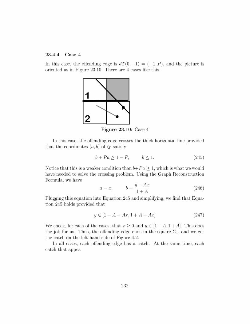
23.4.4 Case 4

In this case, the offending edge is dT (0,−1) = (−1, P ), and the picture isoriented as in Figure 23.10. There are 4 cases like this.

1

2

Figure 23.10: Case 4

In this case, the offending edge crosses the thick horizontal line providedthat the coordinates (a, b) of ζΓ satisfy

b+ Pa ≥ 1− P, b ≤ 1. (245)

Notice that this is a weaker condition than b+Pa ≥ 1, which is what we wouldhave needed to solve the crossing problem. Using the Graph ReconstructionFormula, we have

a = x, b =y − Ax1 + A

(246)

Plugging this equation into Equation 245 and simplifying, we find that Equa-tion 245 holds provided that

y ∈ [1− A− Ax, 1 + A+ Ax] (247)

We check, for each of the cases, that x ≥ 0 and y ∈ [1−A, 1+A]. This doesthe job for us. Thus, the offending edge ends in the square Σ1, and we getthe catch on the left hand side of Figure 4.2.

In all cases, each offending edge has a catch. At the same time, eachcatch that appea

232

24 Computer Assisted Techniques

24.1 Operations on Polytopes

Clean Polytopes: Say that a clean polytope is a convex polytope in R4

with integer vertices, such that each vertex is the unique extreme point ofsome linear functional. In ther words, a clean polytope is the convex hull ofits (integer) vertices, and the convex hull of any proper subset of vertices isa proper subset. We always deal with clean polytopes. The polytopes in theplaid and graph triple partitions have all the properties mentioned above,except that their vertices are rational rather than integral. We fix this prob-lem by scaling all polytopes in all partitions by a factor of 60.

Clean Polytope Test: Suppose we are given a finite number of integerpoints in R4. Here is how we test that they are the vertices of a cleanpolytope. We consider all linear functionals of the form

L(x, y, z, A) = c1x+ c2y + c3z + c4A, |ci| ≤ N (248)

and we wait until we have shown that each vertex is the unique maximumfor one of the functionals. For the polytopes of interest to us, it suffices totake N = 3. In general, our test halts with success for some N if and only ifthe polytope is clean.

Disjointness Test: Here is how we verify that two clean polytopes P1 andP2 have disjoint interiors. We consider the same linear functionals as listedin Equation 248 and we try to find some such L with the property that

maxv∈V (P1)

L(v) ≤ minv∈V (P2)

L(v). (249)

Here V (Pk) denotes the vertex set of Pk. If this happens, then we have founda hyperplane which separates the one polytope from the other. This time wetake N = 5.

Containment Test: Given clean polytopes P1 and P2, here is how weverify that P1 ⊂ P2. By convexity, it suffices to prove that v ∈ P2 for eachvertex of P1. So, we explain how we verify that P = P2 contains an integerpoint v. We do not have the explicit facet structure of P , though for anotherpurposes (computing volumes) we do find it.

233

Let Lk denote the set of all linear functionals determined by 4-tuples ofvertices of P . Precisely, Given 4 vertices of P , say w0, w1, w2, w3, and someinteger point v, we take the 4× 4 matrix whose first three rows are wi − w0

for i = 1, 2, 3 and whose last row is v. Then

Lw0,w1,w2,w3(v) = det(M) (250)

is the linear functional we have in mind.If the vertices do not span a 3-dimensional space, then L will be trivial.

This does not bother us. Also, some choices of vertices will not lead to linearfunctions which define a face of P . This does not bother us either. Thepoint is that our list of linear functionals contains all the ones which do infact define faces of P . We take our vertices in all orders, to make sure thatwe pick up every possible relevant linear functional. The computer does notmind this redundancy.

It is an elementary exercise to show that v 6∈ P if and only if v is a uniqueextreme point amongst the set v ∪ V (P ) for one of our linear functionals.Here V (P ) denotes the vertex set of P , as above. So, v ∈ P is and only if vis never a unique extreme point for any of the linear functionals on our list.

Volume: First we explain how we find the codimension 1 faces of P . Wesearch for k-tuples of vertices which are simultaneously in general positionand the common extreme points for one of the linear functionals on our list.As long as k ≥ 4, the list we find will be the vertices of one of the faces of P .

Now we explain how we compute the volume of P . This is a recursiveproblem. Let v0 be the first vertex of P . Let F1, ..., Fk be the codimension 1faces of P . Let Pj be the cone of Fj to v0. This is the same as the convexhull of Fj ∪ v0. Then

vol(V ) =k∑

j=1

vol(Vj). (251)

If v0 ∈ Vj then the volume is 0. These extra trivial sums do not bother us.To compute vol(Vj) we let wj0, wj1, wj2, wj3 be the first 4 vertices of Fj.

Let Lj be the associated linear functional. Then

4× vol(Vj) = Lj(v0 − wj0)× vol(Fj). (252)

We compute vol(Fj) using the same method, one dimension down. Thatis, we cone all the facets of Fj to the point wj0. It turns out that the

234

polyhedra Fij in the subdivision of F are either tetrahedra or pyramidswith quadrilateral base. In case Fij is a tetrahedron we compute 12vol(Fij)by taking the appropriate determinant and doubling the answer. In the othercase, we compute 6 times the volume of each of the 4 sub-tetrahedron of Fij

obtained by omitting a vertex other than w0j and then we add up thesevolumes. This computes 12vol(Fij) regardless of the cyclic ordering of thevertices around the base of Fij.

When we add up all these contributions, we get 12 vol(Fj). So, our finalanswer is 48 vol(V ). The reason we scale things up is that we want to haveentirely integer quantities.

Potential Overflow Error: With regard to the volume method, a straight-forward application of our method can cause an overflow error. We do thecalculations using longs (a 64 bit representation of an integer) and the totalnumber we get by adding up 218 smaller numbers is (barely) too large to bereliable represented. However, we observe that all the numbers we computeare divisible by 480. So, before adding each summand to the list, we divideout by 480. This puts us back into the representable range. Recalling thatwe have scaled up by 60, then computed 48 times the volume, then dividedby 480, our final computation is

Ω = 64103 (253)

times the true volume.

24.2 The Calculations

We work with 3 partitions and then a few extra polytopes.

The Plaid Partition: The plaid partition, described in §7 has 26 cleanpolytopes modulo the action of the plaid lattice Λ1. For each all i, j, k with|i|, |j|, |k| ≥ 3, we check that each polytope Pk is disjoint from λi,j,k(Pℓ),where λi,j,k is the standard word in the generators of Λ1. Given that allthe original polytopes intersect the fundamental domain, and given the sizesof the translations in Λ1, this check suffices to show that the orbit Λ(

⋃Pi)

consists of polytopes with pairwise disjoint interiors and that the union ofour polytopes P0 ∪ ... ∪ P25 is contained in a fundamental domain for Λ1.

235

At the same time, we compute that

25∑

i=0

vol(Pi) = 8. (254)

Again, we compute that the scaled volume is 8Ω. This coincides with thevolume of the fundamental domain [−1, 1]3 × [0, 1] for Λ1.

We now know the following three things:

1. The union of the 26 plaid polytopes is contained in a fundamentaldomain.

2. The union of the 26 plaid polytopes has the same volume as a funda-mental domain.

3. The Λ1 orbit of the 26 plaid polytopes consists of polytopes havingpairwise disjoint interiors.

We conclude from this that the Λ1 orbit of the plaid polytopes P0, ..., P25 isa partition of X, as desired.

Remark: In view of the fact that we have already proved the Plaid MasterPicture Theorem, these checks are really unnecessary, provided that we havecorrectly interpreted the geometric description of the plaid polytopes andcopied down the points correctly. So, these calculations really serve as sanitychecks.

The Graph Partitions: We just deal with the (+) graph partition, be-cause the (−) graph partition is isometric to the (+) partition. We makeall the same calculations for the (+) graph partition that we made for theplaid partition, and things come out the same way. Once again, the fact thatthings work out is a consequence of our Master Picture Theorem from [S0],but we made several changes to the polytopes in this paper. We swappedthe first and third coordinates, and also translated. So, these calculationsserve as sanity checks.

The Reduced Plaid Triple Partition: The reduced plaid triple parti-tion consists of 218 convex rational polytopes, which we scale up by a factorof 60. The scaled polytopes are all clean. Using the above tests, we check

236

that the polytopes have pairwise disjoint interiors, and are all contained inthe fundamental domain XΠ = [−1, 1]3 × [0, 1]. Finally, we check that thesum of the volumes is 8. This verifies that we really do have a partition.

There is one more important check we make. Each plaid triple polytopehas a 6 letter code which tells how it is obtained as an intersection of theform A−1 ∩ A0 ∩ A1, where Ak is a polytope in the partition F (k)(P). HereP is the plaid partition and F is the curve-following dynamics.

We check that each triple plaid Πk is contained in the three polytopesthat are supposed to contain it, and is disjoint from all the others in theplaid partition and its images under the forward and backward curve fol-lowing map. This verifies that the plaid triple partition really is as we havedefined it.

Nine Graph Doubles: We mentioned in §21 that sometimes it happensthat Ψ(Πk) is not contained in a single graph polytope of one of the twopartitions, but rather a union of two of them. This happens 19 times forthe (+) partition and 19 times for the (−) partition. We call these unions ofgraph polytopes doubles .

We check that each graph double (when scaled up by a factor of 60) isclean, that each graph double indeed contains both of its constituent graphpolytopes, and that the volume of the graph double is the sum of the vol-umes of the two constituents. This shows that the union of the two graphpolytopes really is a clean convex polytope.

The Rest of the Calculations Each edge crossing problem either involvesshowing that some linear functional is positive on a polytope, or else thattwo clean polytopes have pairwise disjoint interiors, or that one clean poly-tope is contained in another. We simply run the tests and get the outcomesmentioned above. The same goes for the several recalcitrant cases done inconnection with the proof of Statement 5 of the Pixellation Theorem givenin the last chapter. Finally, checking that there are no errant edges justamounts to listing out the data and checking that there are no forbiddenedge assignments. We also survey the assignments visually and see thatthere are no errant edges.

237

24.3 The Computer Program

In this last section I’ll give a rough account of some of the main features ofthe program. The main purpose of this account is to show you the kindsof things the program can do. The later entries in this section are rathersketchy. They are designed to let you know what sorts of things the programcan do, but they stop short of giving detailed instructions on how to get theprogram to do it. The program has its own documentation - every feature isexplained - and this should help with the details.

24.3.1 Downloading the Program

My computer program can be downloaded from

http://www.math.brown.edu/∼res/Java/PLAID2.tar

When you download the file, you get a tarred directory. I untar the directorywith the Unix command tar -xvf PLAID2.tar. (Your system might bedifferent.) Once this is done, you have a new directory called PlaidModel.The program resides in this directory and is spread out among many files.

24.3.2 Running and Compiling

The file Main.java is the main file. Assuming that the program is compiledalready (and you would know by the presence of many .class files) compile theprogram with the command javac *.java and then you run the program withthe command java Main. All this assumes, of course, that your computercan run Java programs. If everything works, a small and colorful windowshould pop up. This is the control panel. You can launch the other parts ofthe program from this window.

24.3.3 What to do first

The control panel has a smaller window which lists 10 pop-up windows. Ifyou click on these buttons, additional windows will pop up. The first buttonyou should press is the Document button. This will bring up a windowwhich has information about the program. If you read the documentation,you will see how to operate the program.

238

24.3.4 Presets

The program has 4 preset modes. When you select the preset option on themain control panel, you bring up an auxiliary control panel called presets.This panel has 4 buttons:

• quasi-isomorphism theorem

• plaid master picture theorem

• graph master picture theorem

• plaid-graph correspondence

If you press one of these buttons, various windows will pop up, and theywill be automatically set up to best show the advertised features. Moreober,documentation will appear which gives further instructions and explanations.

There is one irritating feature of the program which I should mention.The preset features work best when all the auxiliary pop-up windows areclosed. If you press a preset when some the pop-up windows are alreadyopen, you run the risk of having duplicate windows open, and this causesproblems for the program. When you want to use one of the preset buttons,you should close all the auxiliary windows.

24.3.5 Surveying the Data and Proofs

The files starting Data contain all the data for the polytope partitions. Thefile names give some idea of what the files contain. For instance, Data-GraphPolytopes.java contains the coordinates of the graph PET poly-topes. Some of the files are harder to figure just from the names, but thefiles themselves have documentation.

The files starting Proof contain all the routines for the proof. Again,the names indicate the tests contained in the files. For instance ProofVol-ume.java contains the volume calculations for the partitions.

239

Part V

The Distribution of Orbits

240

25 Unbounded Orbits

25.1 Geometric Limits

We start with an irrational A ∈ (0, 1) and we seek a good offset V ∈ R3×0such that the tiling defined by ΘA,V has a fat component – i.e. a curve notcontained in the tubular neighborhood of any line. We don’t care about thedirections of the components of the tiling, so we take the domain of ΘA tobe X1. We drop the 4th coordinate for convenience.

Our basic idea is to take geometric limits of the big polygons produced in§3.1. Suppose that Ak = pk/qk is a sequence of even rational parametersconverging to some irrational parameter A. Let Γk denote the big polygonassociated to Ak.

We set Θk = ΘAkfor ease of notation. The maps Θk converge, uniformly

on compact sets, to ΘA. However, the limit map ΘA is not useful to usbecause the distance between the closest point on Γk and the origin tends to∞ with k. Also, ΘA(G) will intersect the walls of the partition. We need amore robust kind of limit.

Define the anchor of Γk to be the set 〈Γk〉 ⊂ G consisting of centers oftiles involved in Γk which have the form (1/2, y). Let Z = zk be a sequencewhere zk ∈ 〈Γk〉. Define

ΘZk (c) = Θk(c+ zk). (255)

The map ΘZk behaves near the origin like Θk behaves near zk. Since Θk is

locally affine, there is some vector Vk such that ΘZk = Θk,Vk

. Passing to asubsequence, we get some offset VZ such that

limk→∞

ΘZk = ΘA,VZ

. (256)

By construction, the paths Γk − zk will converge to an unbounded path thatinvolves the tile centered at (1/2, 1/2).

The trick is finding a sequence Z so that VZ is a good offset. One suchsequence is given by zk = (1/2, τk + 1/2), where τk is as in §1.1. However,this choice never leads to a good offset. Our idea is to pick a rational ap-proximation so that the sets 〈Γk〉 are huge in the sense that the finite setΘk(〈Γk〉) becomes dense in a Cantor set as k →∞. This structure will allowus to get good offsets in the limit, and the limiting tiling will turn out tohave a fat path.

241

25.2 Approximating Irrationals

Our first step is to find a good sequence pn/qn of even rationals that limitsto A. The sequence we choose is related to, but distinct from, the sequenceof continued fraction approximants. (The continued fraction approximantsare not always even rationals.) We defer the proofs of the technical lemmasto the next chapter.

Even Predecessors: Two rationals a1/b1 and a2/b2 are called Farey re-lated if |a1b2 − a2b1| = 1. Let p′/q′ and p/q be two even rational paramters.We write p′/q′ ← p/q if p/q and p′/q′ are Farey related and ω′ < ω. Hereω = p + q as usual. We call p′/q′ the even predecessor of p/q. This rationalis unique.

Core Predecessors: Let τ ∈ (0, ω/2) be as in §1.1. We define κ ≥ 0to be the integer so that

κ

2κ+ 1≤ τ

ω<

κ+ 1

2(κ+ 1) + 1. (257)

We only get equality on the left hand side when p/q = 1/2n. In this case,τ = 1. Define

p = p− 2κp′, q = q − 2κq′. (258)

We will see in the next chapter that p/q is an even rational in (0, 1). We callp/q the core predecessor of p/q. Note that when κ = 0 we have p/q = p/q.We only care about the core predecessor when κ ≥ 1.

Predecessors: Given an even rational parameter p/q, we define the pre-decessor p∗/q∗ as follows:

• If p = 1 then p∗/q∗ = 0/1.

• If p ≥ 2 and κ = 0 then p∗/q∗ = p′/q′, the even predecessor of p/q.

• If p ≥ 2 and κ ≥ 1 then p∗/q∗ = p/q, the core predecessor of p/q.

We write p∗/q∗ ≺ p/q. This definition turns out to be very well adapted tothe plaid model. Lemma 26.1 from the next chapter collects together manyof the relations between these rationals.

242

The Predecessor Sequence: In the next chapter, we will prove the fol-lowing result.

Lemma 25.1 Let A ∈ (0, 1) be irrational. Then there exists a sequencepk/qk such that

• p0/q0 = 0/1

• pk/qk ≺ pk+1/qk+1 for all k

• A = lim pk/qk.

We call pk/qk the predecessor sequence. This terminology suggests thatthe predecessor sequence is unique. However, we will not bother to provethis. We just need existence, not uniqueness.

Diophantine Result: Let pk/qk be the predecessor sequence converg-ing to A. We classify a term pk/qk in the predecessor sequence as follows:

• weak: τk+1 < ωk+1/4. Here κk+1 = 0.

• strong: τk+1 ∈ (ωk+1/4, ωk+1/3). Here κk+1 = 0.

• core: τk+1 > ωk+1/3. Here κk+1 ≥ 1.

Lemma 25.2 The predecessor sequence has infinitely many non-weak terms.For each non-weak term pk/qk, we have

∣∣∣A− pkqk

∣∣∣ < 48

q2k.

The Approximating Sequence: We define the approximating sequenceto be the set of terms pk/qk in the predecessor sequence such that either

• pk/qk is core.

• pk/qk is strong and pk−1/qk−1 is not core.

If there are infinitely many core terms in the predecessor sequence, thenthe approximating sequence contains all of these. If there are only finitelymany core terms in the predecessor sequence, then there are infinitely manystrong terms, and the approximating sequence contains all but finitely manyof these. So, in all cases, the approximating sequence is an infinite sequence.

243

25.3 Arc Copying

Let Rp/q denote the rectangle bounded by the bottom, left, and top of thefirst block, and by whichever vertical line of capacity at most 4 is closest tothe left edge of the first block. Let γp/q denote the subset of Γp/q containedin the box Rp/q. When the dependence on the parameter is implied we willsuppress it from our notation. In subsequent chapters, we prove the followingresult.

Lemma 25.3 (Box) For any even rational parameter p/q, the set γp/q isan arc whose endpoints lie on the right edge of Rp/q.

Figure 8.2 shows the big polygons associated to two different parameters.Notice that the polygon Γ12/29 copies some of Γ5/12. The boxes B5/12 andB12/29 are the first columns (i.e. the union of the leftmost 3 sub-rectangles)of the tic-tac-toe grids shown in each of the two pictures.

Figure 8.2: Arc copying for 5/12 and 12/29.

Let TH and BH denote the top and bottom horizontal lines of capacity2 with respect to some rational parameter. In the statement of the resultsbelow, it will be clear which parameters these lines depend on. In the subse-quent chapters we prove the following result.

Theorem 25.4 (Copy) Let p0/q0, p1/q1 be two successive terms in the ap-proximating sequence. Then there is some vertical translation Υ such thatthat Υ(R0) is contained below the horizontal midline of R1, and Υ(γ0) ⊂ γ1.Moreover, either Υ(BH0) = BH1 or Υ(TH0) = BH1.

244

The Copy Theorem has a more symmetric formulation. Let η = ω − 2τ .Geometrically η is the vertical distance between lines BH and TH.

Corollary 25.5 Let p0/q0, p1/q1 be two successive terms in the approximat-ing sequence. Then there are vertical translations ΥB and ΥT such that

ΥB(γ0) ⊂ γ1, ΥT (γ0) ⊂ γ1.

The image ΥB(γ0) lies below the horizontal midline of B1 and The imageΥT (γ0) lies above the horizontal midline of B1. Furthermore

ΥT (∗)−ΥB(∗) = (0, η1 ± η0).

Proof: We set ΥB = Υ from the Copy Theorem. Let Rj denote reflectionin the horizontal midline of Bj. Note that Rj(γj) = γj. We let

ΥT = R1 ΥB R2.

By symmetry ΥT (γ0) ⊂ γ1 and the image lies above the horizontal midlineof B1.

If ΥB(BH0) = BH1 then ΥT (TH0) = TH1. In this case

ΥT (∗)−ΥB(∗) = η1 − η0.If ΥB(TH0) = BH1 then ΥT (BH0) = TH1. In this case

ΥT (∗)−ΥB(∗) = η1 + η0.

Either case gives us the final statement of the corollary. ♠

Corollary 25.6 〈Γ1〉 contains two copies of 〈Γ0〉, separated by one of thetwo vectors (0, η1 ± η0).

We can iterate this result. Let Γk be the big polygon corresponding tothe kth term in the approximation sequence.

Corollary 25.7 〈Γk〉 contains 2k points of the form

ck +k−1∑

i=0

ǫi(0, di),

where di is one of the two terms ηi+1− ηi for each i. Here ck is some integerand ǫi is any binary sequence of length k.

245

25.4 The Images of the Anchors

In this section we prove a result about the images of the anchors. We keepthe notation from the previous section. First we make some preliminaryobservations. For any parameter A, a fundamental domain for X1 is [−1, 1]3.The coordinates on this space are (T, U1, U2). We think of this space as afibration over the T coordinate. The (U1, U2) fibers are all flat square tori.Let γP denote the geodesic in the fiber over T = P which has slope −1. HereP = 2A/(1 + A) as usual. To simplify notation, we set γk = γPk

.Let Y = 1/2 × Z. Using the formula for Θk we see that Θk(Y ) ⊂ γk.

DefineIk = Θk(〈Γk〉) ⊂ γk (259)

The last containment comes from the fact that 〈Γk〉 ⊂ Y , by definition. FromCorollary 25.7 we know that Ik has at least 2k points, namely

Θk(ck) +k−1∑

i=0

ǫi Θk(0, di), ǫ0, ..., ǫk−1 ∈ 0, 1. (260)

The addition on the right takes place in the flat square torus above the fiberT = Pk.

Now we are going to analyze the terms in Ik and show that, on a subse-quence, the sequence of sets Ik converges to a Cantor set. We will interpretthis Cantor set as a subset of the available offsets we can get by taking thekind of limit discussed in §25.1.

Lemma 25.8 As k →∞, the vectors Θk(0, di) converge to ΘA(0, di).

Proof: We have

Θk(0, di) = (2di, 0, 2diPk) ≡ (0,−diPk,+diPk) mod Λ1. (261)

Using Lemma 25.2 and the fact that the map x → 2x/(x + 1) is 2-lipschitzon (0, 1), we have

‖Pk − P‖ ≤96

ω2k

. (262)

The lemma follows immediately from this estimate and from the fact that|di| ≤ 2ωk once k ≥ i. ♠

246

The vectors ΘA(di) are growing unboundedly long, but mod Λ1 thesevectors converge to 0 exponentially fast. That is the same kind of convergencewe are after here.

Lemma 25.9 ‖ΘA(0, di)‖ < C2−i mod Λ1 for some constant C.

Proof: By the Copy Theorem, ωk < ωk+1/2. Hence ωi ≥ 2i. So, it sufficesto prove that

‖ΘA(0, di)‖ <C

ωi

,

for some constant C. By the triangle inequality and Equation 262, it sufficesto prove that

‖Θi(0, ηi)‖ <C

ωi

.

We haveΘi(0, ηi) = (0,−Piηi, Piηi). (263)

We have

ηiPi = (ωi − 2τi)Pi = 2pi −4τipiωi

= 2pi − 2ai −2

ωi

.

Here ai is some integer. This means that

Piηi =2

ωi

mod 2Z. (264)

Our result follows from Equations 263 and 264. ♠

Combining the results above, we can say that Ik is becoming dense in theCantor set

∞∑

i=0

ǫiΘA(0, di), ǫi ∈ 0, 1. (265)

Every infinite sum makes sense because the terms decay exponentially fast.The sequence of translations is given by ΘA(ck).

In the next section we use this result to finish the proof of the UnboundedOrbits Theorem.

247

25.5 The End of the Proof

Here we give a criterion for V to be a good offset. Define

Q[P ] = r1 + r2P | r1, r2 ∈ Q. (266)

Lemma 25.10 If V = (P, u1, u2) with u1, u2 6∈ Q[P ], Then V is a goodoffset.

Proof: The (U1, U2) fiber over and point of Q[P ] intersects the walls ofour partition in rectangles bounded by lines defined over Q[P ]. This is aconsequence of the fact that the 4-dimensional polytopes of our partition areintegral. Given c ∈ G, which has half-integer coordinates (m+1/2, n+1/2),we compute

ΘA,V (c) = (2mP +P, 2mP +P, 2mP +P )+ (2n+1, 0, 2nP +P )+V. (267)

The first coordinate always lies in Q[P ] and the second two coordinates neverdo. Hence, this point never lies in the boundary of the partition. ♠

Now we go back to our idea of choosing zk ∈ 〈Γk〉 and taking a geometriclimit of the maps ΘZ

k where Z = zk.

Lemma 25.11 There exists a sequence Z = zk with zk ∈ 〈Γk〉 such thatthe some subsequential limit VZ is a good offset.

Proof: Passing to a subsequence, we can assume that ΘA(ck) converges modΛ1 to come vector V . On this subsequence, the sets Ik are becoming densein the Cantor set

Ω = V +∞∑

i=0

ǫiΘA(0, di), ǫi ∈ 0, 1. (268)

Ω lies the geodesic γp, which lies in the fiber over T = P and has slope −1in the (U1, U2) plane. In particular, the set in Equation 268 contains pointsof the form (P, u1, u2), where neither u1 nor u2 belongs to Z[P ]. In otherwords, according to Lemma 25.10, the Cantor set Ω contains vectors whichare good offsets. But this means that there exists a sequence Z such thatΘk(zk) → VZ where VZ is a good offset. But Θk(zk) = ΘZ

k (0, 0). In other

248

words, VZ is a good offset. ♠

We choose such a sequence and take a limit. Let ΘA,V be the limitingmap. Since V is a good offset, the tiling associated to ΘA,V is entirely welldefined. By construction, the curve Γ∞ of the tiling through (1/2, 1/2) isunbounded. However, we can say more than this. There are infinitely manyindices for which some initial portion of Γ∞ agrees with Γk ∩Rk. Here Rk isthe box from the Copy Lemma. But this means that the projection of Γ∞onto the x-axis exceeds pk/2 for infinitely many k. Hence the projection ofΓ∞ onto the x-axis is unbounded. At the same time, 〈Γ∞〉 is infinite. Thisis to say that Γ∞ contains infinitely many points which are within 1/2 of they-axis. These two properties together imply that Γ∞ is fat. This completesthe proof of the Unbounded Orbits Theorem.

249

26 Some Elementary Number Theory

In this chapter we will justify all the statements quoted in §25.2. We will alsoprove a number of other technical results which establish useful identities andinequalities between the rationals discussed in §25.2.

26.1 All About Predecessors

We fix an even rational parameter p/q. To avoid trivialities, we assume thatp > 1. We recall the following definitions from §25.2.

• ω = p+ q.

• τ ∈ (0, ω/2) is the unique solution to 2pτ ≡ ±1 mod ω.

• κ ∈ 0, 1, 2, ... is such that

κ

2κ+ 1≤ τ

ω<

κ+ 1

2(κ+ 1) + 1. (269)

• p′/q′ is the even predecessor of p/q. That is, |pq′− qp′| = 1 and q < q′.

• p/q is the core predecessor of p/q. Here p = p− 2κp′ and q = p− 2κq′.

We mean to define ω, τ, κ for the other parameters as well. Thus, for instance,ω′ = p′ + q′.

Lemma 26.1 The following is true.

1. p/q ∈ (0, 1) is an even rational in lowest terms.

2. Either τ − τ ′ = κω′ or τ + τ ′ = (1 + κ)ω′. In all cases, τ ′ ≤ τ .

3. p′/q′ is the even predecessor of p/q.

4. κ = 0.

5. ω − 2τ = ω − 2τ .

6. If κ = 0 then τ ′ = τ when τ < ω/4 and τ ′ = ω′ − τ when τ > ω/4.

7. ω ≤ (3/(3 + 2κ))ω.

250

26.1.1 Statement 1

We first give a formula for p′/q′. There is some integer θ > 0 so that

2pτ = θ(p+ q)± 1. (270)

Since q > 1 we have θ < 2τ . We also have θ ≤ p. The case θ = p forcesp = 1. Hence θ < min(p, 2τ). Rearranging Equation 270 we get

|pq′′ − qp′′| = 1, p′′ = θ, q′′ = 2τ − θ.

This implies that p′′/q′′ is in lowest terms. Moreover, both p′′ and q′′ are odd.Hence

p′ = p− p′′ = p− θ, q′ = q − q′′ = q − 2τ + θ. (271)

This gives us

ω′ = ω − 2τ ≤ ω − 2ωκ

2κ+ 1=

ω

2κ+ 1. (272)

Rearranging this, we get

2κp′ + 2κq′ + (p′ + q′) ≤ p+ q. (273)

Given that |pq′− qp′| = 1, Equation 273 forces 2κp′ < p and 2κq′ < q. Hencep = p − 2κp′ > 0 and q = q − 2κq′ > 0. Since p/q is Farey related top′/q′ ∈ (0, 1), we see that p/q also lies in (0, 1) and is in lowest terms. Sincep/q is an even rational, so is p/q. This proves Statement 1.

26.1.2 Statement 2

We use the formulas derived in the previous section. Let θ be as above.Choosing the sign as in Equation 270, we have

θω′ ± 1 = θ(ω − 2τ)± 1 = (θω ± 1)− 2θτ = 2pτ − 2θτ = 2p′τ. (274)

This shows that 2p′τ ≡ ±1 mod ω′. But, by definition, 2p′τ ′ ≡ ±1 mod ω′.Hence 2p′τ ≡ ±2p′τ ′ mod ω′. Since 2p′ is relatively prime to ω′ we see that

τ ≡ ±τ ′ mod ω′. (275)

If τ ≡ τ ′ mod ω′ then τ ′ = τ − κω′ provided that this expression lies in(0, ω′). We compute

τ − κω′ = τ − κ(ω − 2τ) = (2κ+ 1)τ − κω > 0 (276)

251

τ − (κ+ 1)ω′ = τ − (κ+ 1)(ω − 2τ) = (2κ+ 3)τ − (κ+ 1)ω < 0 (277)

These two inequalities show that τ − κω′ ∈ (0, ω′). In this case it is obviousthat τ ′ ≤ τ .

When τ ≡ −τ mod ω, a similar argument shows that

(κ+ 1)ω′ − τ ∈ (0, ω′),

and this forces τ ′ = (κ+1)ω′−τ . In this case, the two inequalities τ+τ ′ ≥ ω′

and τ ′ < ω′/2 estabish τ ′ < τ .

26.1.3 Statements 3 and 5

Let p/q be the core predecessor of p/q. Since p = p−2κp′ and q = q−2κq′ thetwo rationals p′/q′ and p/q are both Farey related. Equation 272, which is astrict inequality when p > 1, says that (2κ+ 1)ω′ < ω. Since ω = ω − 2κω′,we conclude that ω′ < ω. Hence p′/q′ is the even predecessor of p/q.

Since p′/q′ is the even predecessor of both p/q and p/q, Equation 272 tellsus that ω − 2τ = ω′ = ω − 2τ . Hence ω − 2τ = ω − 2τ .

26.1.4 Statement 4

If Statement 4 is false, then Equation 272, applied to to the pair (p/q, p′/q′),gives

ω − 3ω′ > 0. (278)

Combining this with the fact that

ω = ω − 2κω′ > 0,

we can say thatω − (2κ+ 3)ω′ > 0.

But then we have

1

2κ+ 3< 1− 2

( τω

)=ω′

ω<

1

2κ+ 3.

This is a contradiction.

252

26.1.5 Statement 6

When κ = 0, Statement 1 says that either τ = τ ′ or τ + τ ′ = ω′. Also, fromEquation 272 we see that 2ω′ < ω if and only if τ > ω/4.

Suppose that τ ′ = τ and τ > ω/4. Then

τ = τ ′ < ω′/2 < ω/4.

This is a contradiction. So, τ ′ = τ implies that τ < ω/4. Suppose thatτ ′ = ω′ − τ and τ < ω/4. Then

2τ > 2τ ′ = 2ω′ − 2τ > ω − 2τ.

This gives τ > ω/4, a contradiction. So, τ ′ = ω − τ implies that τ > ω/4.

26.1.6 Statement 7

We have

ω = ω − 2κω′ = ω − 2κ(ω − 2τ) = (1− 2κ)ω + 4κτ.

By definitionτ

ω<

κ+ 1

2κ+ 3.

Henceω

ω= 1− 2κ+ 4κ

τ

ω≤ 1− 2κ+ 4κ

κ+ 1

2κ+ 3=

3

3 + 2κ.

26.2 Existence of the Predecessor Sequence

We begin by proving the existence of an auxiliary sequence. The notationp′/q′ ← p/q means that p′/q′ is the even predecessor of p/q.

Lemma 26.2 Let A ∈ (0, 1) be irrational. There exists a sequence pn/qnconverging to A such that pn/qn ← pn+1/qn+1 for all n.

Proof: Let H2 denote the upper half-plane model of the hyperbolic plane.We have the usual Farey triangulation ofH2 by ideal triangles. The geodesicsbounding these triangles join rationals p1/q1 and p2/q2 such that |p1q2 −p2q1| = 1. We call these geodesics the Farey Geodesics . Two of the Fareygeodesics in the tiling join the points 0/1 and 1/1 to 1/0. This last point

253

is interpreted as the point at infinity in the upper half plane model of H2.Let Y = (x, y)| 0 < x < 1 be the open portion of H2 between these twovertical geodesics.

Each Farey geodesic in Y which joins two even rationals p/q and p′/q′

can be oriented so that it points from p/q to p′/q′ if and only if p′/q′ ← p/q.We leave the rest of the Farey geodesics unoriented.

We claim that there is a backwards oriented path from 0/1 to A. Tosee this, choose any sequence of even rationals converging to A and considertheir sequence of even predecessors. This gives us a sequence of finite di-rected paths joining 0/1 to rationals which converge to A. Given the localfiniteness of the Farey triangulation – meaning that any compact subset ofH2 intersects only finitely many triangles – we can take a limit of thesepaths, at least on a subsequence, and get a directed path converging to A.

Reading off the vertices of this path gives us a sequence pn/qn withpn/qn ← pn+1/qn+1 for all n. ♠

Proof of Lemma 25.1: We get the predecessor sequence from the sequencein Lemma 26.2 in the following way. Before each term pn/qn with κn ≥ 1we insert the rational pn/qn. This is the core predecessor of pn/qn. We knowfrom the lemma above that κn = 0 and that pn−1/qn−1 is the predecessor ofpn/qn. In short

pn−1/qn−1 ≺ pn/qn ≺ pn/qn.

Once we make all these insertions, the resulting sequence is a predecessorsequence which converges to A. Again, we will not stop to prove uniquenessbecause we don’t care about it. ♠

26.3 Existence of the Approximating Sequence

We call the sequence from Lemma 26.2 the even predecessor sequence. As wehave just remarked, the even predecessor sequence is a subsequence of thepredecessor sequence.

Lemma 26.3 Let pn/qn be the even predecessor sequence which convergesto A. There are infinitely many values of n such that τn+1 > ωn+1/4.

Proof: If this lemma is false, then we might chop off the beginning andassume that this never happens. We have the formula ωn = ωn+1−2τn+1. So,

254

if this lemma is false then we have 2ωn < ωn+1 only finitely often. Choppingoff the beginning of the sequence, we can assume that this never occurs.

We never have 2ωn = ωn+1 because ωn+1 is odd. So, we always haveωn > ωn+1. In this case, we have

rn−1 = 2rn − rn+1

for r ∈ p, q. Applying this iteratively, we get that rk = (k + 1)r1 − kr0 fork = 1, 2, 3, .... But then lim pn/qn = (p1 − p0)/(q1 − q0), which is rational.This is a contradiction.

Now let pn/qn be a term with 2ωn < ωn+1. We will consider the case whenpn/qn < pn+1/qn+1. The other case has a similar treatment. We introducethe new rational

p∗n/q∗n =

pn+1 − pnqn+1 − qn

.

Note that the three rationals pn/qn and pn+1/qn+1 and p∗n/q

∗n form the vertices

of a Farey triangle. Moreover pn+1/qn+1 < p∗n/q∗n because pn+1/qn+1 is the

Farey sum of pn/qn and p∗n/q∗n.

Given the geometry of the Farey graph, we have

A ∈ [pn/qn, p∗n/q

∗n].

Moreover

|pn/qn − p∗n/q∗n| =1

qnq∗n≤ 1

q2n<

4

ω2n

.

The second-to-last inequality comes from the fact that q∗n > qn. ♠

Proof of Lemma 25.2: Let pk/qk be the even predecessor sequence. Ifit happens infinitely often that κk ≥ 1 then there are infinitely many coreterms in the predecessor sequence. Otherwise the predecessor sequence andthe even predecessor sequence have the same tail end. But then the previousresult shows that there are infinitely many values of k for which 2ωk < ωk+1.This gives infinitely many strong terms. Suppose that p/q, p∗/q∗ are twoconsecutive terms in the predecessor sequence, with p/q non-weak.

Case 1: Suppose that p/q and p∗/q∗ are both terms in the even sequence.Then p/q ← p∗/q∗ and τ∗ > ω∗/4. But then 2ω < ω∗, as in the proof ofLemma 26.3. From here, we get the Diophantine estimate from Lemma 26.3.

255

Case 2: Suppose that neither p/q not p∗/q∗ are terms in the even sequence.This case cannot happen because when p∗/q∗ is the core predecessor of somerational and p/q is the core predecessor of p∗/q∗. This contradicts Statement4 of Lemma 26.1.

Case 3: Suppose that p/q is a term of the even sequence but p∗/q∗ isnot. Then the term in the predecessor sequence after p∗/q∗ is p∗∗/q∗∗, whichbelongs to the even sequence. By Statement 3 of Lemma 26.1, we havep/q ← p∗∗/q∗∗. Moreover 2ω < ω∗ < ω∗∗. From here, we get the Diophantineestimate from Lemma 26.3.

Case 4: Suppose that p/q is not a term in the even sequence but p∗/q∗

is. Then p/q is the core predecessor of p∗/q∗. Statement 4 of Lemma 26.1says that κ = 0. Hence the term p′/q′ preceding p/q in the predecessorsequence is the even predecessor of p/q. Since κ = 0, we have τ < ω/3.Using the formula ω′ = ω − 2τ , we see that 3ω′ > ω. At the same timeω′ < ω < 2ω∗. Lemma 26.3 gives us

∣∣∣A− p′

q′

∣∣∣ < 4

(ω′)2<

36

ω2.

At the same time ∣∣∣pq− p′

q′

∣∣∣ = 1

qq′<

4

ωω′<

12

ω2.

The result in this case then follows from the triangle inequality. ♠

26.4 Another Identity

Let p/q be an even rational parameter with κ ≥ 1. Let p/q be the corepredecessor. Define

w = τ , h = ω − 2τ. (279)

Here is an identity between these quantities.

Lemma 26.4(2κ+ 1)h+ 2w = ω. (280)

256

Proof: DefineFκ =

κ

2κ+ 1. (281)

Let F be the union of all such rationals.We rescale the first block so that it coincides with the unit square. This

rescaling amounts to dividing by ω. For each quantity λ defined above, welet λ∗ = λ/ω. Within the unit square, our identity is

(2κ+ 1)h∗ + 2w∗ = 1. (282)

The rescaled horizontal and vertical lines depend continuously on the param-eter τ ∗. Moreover, when τ ∗ ∈ (Fκ, Fκ+1) is rational, all the horizontal andvertical lines of capacity up to 4κ+ 2 are distinct, because the denominatorof the corresponding rational is at least 2κ + 1. Therefore, κ is a locallyconstant function of τ ∗, and changes only when τ ∗ passes through a value ofF .

Consider what happens when τ ∗ = Fκ + ǫ, and ǫ ∈ (0, Fκ+1 − Fκ). Wecompute

(2κ+ 1)τ ∗ − κ = (2κ+ 1)ǫ < 1/2 (283)

Hence w = (2κ + 1)ǫ, which means that 2w∗ = (4κ + 2)ǫ. We also haveh∗ = 1 − 2τ ∗. From these equations one can easily compute that Equation282 holds for all ǫ ∈ (0, Fκ+1 − Fκ). ♠

Lemma 26.5 w = τ . In other words, the line x = τ has capacity 4κ + 2with respect to p/q.

Proof: In view of Equation 280, we just have to prove that

(2κ+ 1)(ω − 2τ) + 2τ = ω (284)

By Statement 5 of Lemma 26.1 we have ω−2τ = ω−2τ . But then Equation284 is equivalent to

(2κ+ 1)ω − 4κτ = ω. (285)

This equation holds, because

ω − ω = 2κω′ = 2κ(ω − 2τ) = 2κ(ω − 2τ) = 2κω − 4κτ .

This completes the proof. ♠

257

27 The Box Lemma and The Copy Theorem

27.1 The Weak and Strong Copying Lemmas

In this chapter we reduce the Box and Copy Lemmas from §25.3 to threeother results, the Weak Copy Lemma, the Strong Copy Lemma, and theCore Copy Lemma. We explain the Weak and Strong Copy Lemmas in thissection and the Core Copy Lemma in the next.

Let p/q be an even rational parameter with κ = 0. Let p′/q′ be the evenpredecessor of p/q. Let Π and Π′ denote the plaid tilings with respect tothese two parameters. With κ = 0 there are two subcases.

• weak: 2ω′ > ω. This corresponds to τ < ω/4.

• strong: 2ω′ < ω. This corresponds to τ > ω/4 (and τ < ω/3.)

Let Rp′/q′ be the rectangle associated to the parameter p′/q′ in §25.3.Again, this rectangle is bounded by the lines

• y = 0.

• y = ω′.

• x = 0.

• x = min(τ ′, ω − 2τ ′).

The right side of R′p′/q′ is whichever line of capacity at most 4 is closest tothe y-axis.

In the weak case, we let Σ′ denote the subset of of Rp′/q′ bounded aboveby the line

y = ω′ −min(τ ′, ω′ − 2τ ′). (286)

That is, the top of Σ′ is whichever horizontal line of capacity at most 4 liesclosest to the top of Rp′/q.

In the strong case, we let Σ′ = Rp′/q′ .In both cases we define

Σ = Σ′. (287)

Even though Σ = Σ′ it is useful to have separate notation, so that in generalan object X ′ corresponds to the parameter p′/q′ and an object X correspondsto the parameter p/q.

In the next chapter we will prove the following result.

Lemma 27.1 (Weak and Strong Copying) Σ′ ∩ Π′ = Σ ∩ Π.

258

27.2 The Core Copy Lemma

Let p/q be an even rational parameter with κ ≥ 1. Let p/q be the core

predecessor of p/q. Let Π and Π denote the plaid tilings with respect tothese two parameters.

Let Υ be vertical translation by (ω + ω)/2. It follows from Statement 5of Lemma 26.1 that Υ maps the horizontal lines of capacity ±1 w.r.t p/q tothe lines of capacity ±1 w.r.t. p/q.

Let Rp/q is the rectangle associated to the parameter p/q in §25.3. Define

Σ = Rp/q, Σ = Υ(Σ). (288)

In §9 we will prove the following result.

Lemma 27.2 (Core Copying) Σ ∩ Π = Υ(Σ ∩ Π).

27.3 Proof of the Box Lemma

Our proof goes by induction on the denominator of the parameter. We willsuppose that p/q is a rational with the smallest denominator for which wedon’t know the truth of the result.

By construction, Γ can only intersect ∂R in the right edge, which wecall ρ. If we knew that Γ intersects ρ twice, then, because Γ is a closedloop, we could conclude that the portion of Γ contained in Σ is an arc whoseendpoints are on ρ. If ρ has capacity 2, then Γ can intersect ρ at most twice,and the large x-diameter of Γ implie that Γ does intersect ρ. By symmetry,Γ intersects ρ twice.

Now suppose that ρ has capacity 4. In this situation, we have κ ≥ 1, sowe can apply the Core Copy Lemma to p/q and p/q.

Lemma 27.3 Σ ⊂ R.

Proof: The left edges of Σ and R both lie in the x-axis. So, we just haveto show that the width of Σ is at most the width of R. The width of R isω − 2τ . Statement 2 of Lemma 26.1 says that κ = 0. Hence, the width of Σis τ , a quantity which not greater than ω − 2τ . (The latter quantity is thedistance between the nearest line of capacity 4 to the x-axis.) Now, usingStatement 5 of Lemma 26.1, we observe that τ ≤ ω − 2τ = ω − 2τ. ♠

259

Lemma 27.4 Γ does not intersect the right edge of Σ.

Proof: Since κ = 0, the right edge of Σ has capacity 2. Γ only intersects theline containing this edge twice, and these intersection points must outside ofΣ, for otherwise Γ could not make a closed loop. Compare Figure 2.1. ♠

It now follows from the Core Copy Lemma that Γ does not intersect theright edge of Σ. Figure 10.1 shows three sub-rectangles R1, R2,Σ ⊂ R. Thehorizontal dividers in the picture are the horizontal lines of capacity 2. Wehave already shown that Γ does not intersect the right edge of Σ. But thenΓ cannot cross ρ between the two horizontal lines of capacity 2. To finishour proof, we just have to check that Γ intersects the right edge of R1 once.By symmetry, Γ intersects the right edge of R2 once, and the right edge ofΣ blocks Γ so that it cannot intersect ρ anywhere else.

V

B

Figure 10.1: The rectangles R1, S, R2.

We know that Γ cannot intersect ρ1 more than twice because then, bysymmetry, Γ would intersect ρ at least 6 times. If Γ intersects ρ1 exactlytwice, then Γ is trapped in R1 and cannot get around to close up with theportion of Γ outside R1. Since Γ cannot get trapped in this way, we see thatΓ intersects ρ1 at most once. On the other hand, if Γ does not intersect ρ1at all, then Γ is trapped in the same way. In short, Γ intersects ρ1 exactlyonce, and the same goes for ρ2.

This completes the proof of the Box Lemma.

260

27.4 Setup for the Copying Theorem

Let Rp/q be the rectangle associated to the parameter p/q.

Lemma 27.5 Let p′/q′ be the even predecessor of p/q. Suppose that κ = 0.Then R′ ⊂ R.

Proof: Both boxes contain (0, 0) as the bottom left vertex. So, we just haveto show that the width and height of R′ are at most the width and height ofR. The width of R is τ . The width of R′ is either τ ′ or ω′− 2τ ′, whichever issmaller. In either case, we have width(R′) ≤ τ ′ ≤ τ = width(R). The heightof R is ω and The height of R′ is ω − 2τ . ♠

Suppose that p/q and p∗/q∗ are two consecutive terms in the approximat-ing sequence. We write

p/q = p0/q0 ≺ p1/q1 ← · · · ← pn/qn. (289)

If p/q is strong then p0/q0 is the even predecessor of p1/q1, and pk/qk is weakfor k = 1, ..., n. If p/q is core, then p0/q0 is the core predecessor of p1/q1 andp1/q1 is non-core, and pk/qk is weak for k = 2, ..., n. Here k ≥ 2.

We introduce some notation to help with the proof. Let (Σ′k,Σk+1) bethe pair of rectangles associated to the pair of parameters (pk/qk, pk+1/qk+1).Note that pk/qk gets two such rectangles attached to it, namely Σk and Σ′k.These rectangles play different roles in the proof. Let Πk denote the plaidtiling associated to pk/qk. In general, we set ωk = ω(pk/qk), etc.

27.5 The Strong Case

Suppose first that p0/q0 is strong. Recalling that Σ′0 = Σ1 = B0, we concludethat

B0 ∩ Π0 = Σ′0 ∩ Π0 =∗ Σ1 ∩ Π1 = B0 ∩ Π1. (290)

The starred equality comes from the Strong Copy Lemma.Recall that THk and BHk are the top and bottom horizontal lines of

capacity 2 with respect to pk/qk.

Lemma 27.6 For each k = 1, ..., n the rectangle B0 is contained in the lowerhalf of Bk and one of BH0 or TH0 coincides with BHk.

261

Proof: Note that every box in sight contains (0, 0) as the lower left vertices.So, we can decide which box contains which other box just by looking at thewidths and heights.

Eince τ1 > 1/4 we have 2ω0 < ω1, the height of B0 is less than halfthat of B1. Hence B0 lies in the lower half of B1. By Lemma 27.5, we haveB1 ⊂ ... ⊂ Bk. Hence B0 lies in the lower half of Bk.

From Statement 1 of Lemma 26.1, we have either BH0 = BH1 or TH0 =BH1. From Statement 6 of Lemma 26.1, we see that BH1 = ... = BHk.Hence either BH0 = BHk or TH0 = BHk. ♠

Note that Σ′k contains the lower half of Bk. Hence B0 ⊂ Σ′k for all k.Now we will show inductively that B0 ∩ Πk implies B0 ∩ Πk+1. We alreadyhave proved this for k = 0. For each k = 1, ..., n− 1, we have τk < 1/4. Wehave

B0 ∩ Π0 = B0 ∩ Πk ⊂ Σ′k ∩ Πk =∗ Σk+1 ∩ Πk+1. (291)

The starred equality comes from the Weak Copy Lemma. From this equation,we get B0 ∩ Π0 = B0 ∩ Πk+1. By induction, B0 ∩ Π0 = B0 ∩ Πn. That is,Πn copies Π0 inside B0, and B0 lies in the lower half of Bn. This is what wewanted to prove.

27.6 The Core Case

Suppose that p0/q0 is core. Let Υ be the vertical translation by (ω1−ω2)/2.By construction Υ(B0) is symmetric with respect to the horizontal midlineof B1. Statement 5 of Lemma 26.1 says that the distance between the twohorizontal lines of capacity 2 is the same w.r.t p0/q0 and w.r.t. p1/q1. Hence,by symmetry, Υ(TH0) = TH1 and Υ(BH0) = BH1. We have

Υ(B0 ∩ Π0) = Υ(Σ′0 ∩ Π0) = Σ1 ∩ Π1 = Υ(B0) ∩ Π1. (292)

Lemma 27.7 Υ(B0) ⊂ Σ′1.

Proof: The left edge of Υ(B0) lies in the y-axis, just like the left edge of Σ′1.The width of Υ(B0) is τ0 and the width of Σ′1 is ω1−2τ1. By Statement 2

of Lemma 26.1, the predecessor sequence cannot have 2 core terms in a row.Hence κ0 = 0. This means that 3τ0 < ω0. Hence

τ0 < ω0 − 2τ0 = ω1 − 2τ1.

262

The equality is Statement 5 of Lemma 26.1. This takes care of the widths.The y-coordinate of the top edge of Υ(B0) is (ω0 + ω1)/2. The height of

Σ′1 is either ω1 or 2τ1 depending on whether p1/q1 is strong or weak. Since2τ1 < ω1, we just need to deal with the weak case. That is, we have to showthat ω0 + ω1 < 4τ1. But 4ω1/3 < 4τ1 because p0/q0 is core. So, it suffices toshow that

ω0 < ω1/3.

But this follows from Equation 272, because κ1 ≥ 1. ♠

Now we can take the next step in the argument.

Υ(B0 ∩ Π0) = Υ(B0) ∩ Π1 ⊂ Σ′1 ∩ Π1 =∗ Σ2 ∩ Π2. (293)

The starred equality is either the Weak Copy Lemma or the Strong CopyLemma, whichever applies. Hence Υ(B0 ∩ Π0) = Υ(B0) ∩ Π2.

Lemma 27.8 For each k = 2, ..., n the rectangle Υ(B0) is contained in thelower half of Bk and one of BH0 or TH0 coincides with BHk.

Proof: By Lemma 27.5, the widths of R1, ..., Rk are non-decreasing. So, thewidth of Υ(B0) is at most the width of Rk.

The y-coordinate of the top edge of Υ(B0) is (ω0 + ω1)/2. The height ofB2 is ω2. By Statement 8 of Lemma 26.1, we see that the y coordinate ofthe top edge of Υ(B0) is less than half the height of B2. This takes care ofthe case k = 2.

By Lemma 27.5, we have B2 ⊂ ... ⊂ Bk, and all these boxes have (0, 0)as their bottom left vertex. Hence, Υ(B0) lies in the bottom half of Bk.

We have already seen that Υ(BH0) = BH1 and Υ(TH0) = TH1. ByLemma 27.6, one of these two lines coincides with BH2. But then Statement6 of Lemma 26.1 says that BH2 = ... = BHk. ♠

The rest of the proof is the same inductive argument as in the StrongCase.

263

28 The Weak and Strong Copy Lemmas

28.1 The Mass and Capacity Sequences

In this chapter we prove the Weak and Strong Copy Lemmas. The two resultshave essentially the same proof, except for a few minor details.

Let A = p/q be a paramater and let ω = p+ q as usual. We also remindthe reader that

P =2p

ω=

2A

1 + A, Q =

2q

ω= 2− P. (294)

In this section we repackage some of the results from §1.5. We fix integers1 = x0 < x1 < ω and y0 < y1. We define

Σ = [x0, x1]× [y0, y1], (295)

With this choice of x0 and x1, the rectangle Σ does not intersect the verticalboundry of a block.

All the V lines which intersect Σ have positive capacity. The signs couldbe positive or negative. We define two sequences cj and mj w.r.t. Σ.We have the capacity sequence

cj = [2Pj]2, j = x0, ..., x1. (296)

The terms of the capacity sequence all lie in (−1, 1).We also have the mass sequence

mj = [Pj+1]2, j = y0−2x+1, ..., y1+2x−1, x = x0−x1. (297)

Remarks:(i) Notice that the indices for the mass sequence start below the bottom edgeof Σ (so to speak) and end above it. This is important for us for reasonswhich will become clear momentarily.(ii) We will allow j ∈ ωZ in the mass sequence. Such terms do not have awell-defined sign. The corresponding slanting lines are inert. When we speakof the signs of the terms of the mass sequence, we mean to ignore these terms.(iii) Really we only care about the signs in the mass and capacity sequences,but for the purposes of running certain kinds of arguments it is useful to keeptrack of the numerical values as well.

264

Lemma 28.1 The shade of any vertical intersection point in Σ is determinedby the signs of the terms in the mass and capacity sequences.

Proof: This is just a consequence of the equivalence of the two definitionsof the plaid model. ♠

Corollary 28.2 Suppose that we know how the plaid polygons intersect asingle H line inside Σ. Then the intersection of the plaid polygons with Σ isdetermined by the signs of the mass and capacity sequences.

Proof: We will suppose that we know how the plaid polygons intersect thebottom edge of Σ. The case for any other edge has a similar treatment. LetQ be some unit square in Σ for which we have not yet determined the plaidmodel inside Q. We can take Q to be as low as possible. But then we knowhow the plaid model intersects the bottom edge of Q, and the signs of themass and capacity sequences determine how the tiling intersects the left andright edges. But then the Fundamental Theorem for the plaid model tells usthat ∂Q intersects the plaid polygons in either 0 or 2 points. This allows usto determine how the plaid polygons intersect the top edge of Q. ♠

28.2 A Matching Criterion

In this section, we mean to define all the objects in the previous sectionwith respect to parameter p/q and p′/q′. Our notation convention will bethat the object X corresponds to p/q whenever the same kind of object X ′

corresponds to p′/q′.Let Π denote the union of plaid polygons with respect to p/q and let Π′

denote the union of plaid polygons with respect to p′/q′. Suppose that Σ andΣ′ are rectangles that are equivalent via a vertical translation Υ. That is, Υpreserves the y-axis and Υ(Σ′) = Σ. To be concrete, say that

Υ(x, y) = (x, y + ξ). (298)

We will give a criterion which guarantees that

Υ(Σ′ ∩ Π′) = Σ ∩ Π. (299)

265

Arithmetic Alignment: A necessary condition for Equation 299 is that thesigns of cj are the same as the corresponding signs of c′j and the signsof mj are the same as the corresponding signs of m′j. More precisely,

sign(c′j) = sign(cj+ξ), sign(m′j) = sign(mj+ξ). (300)

We say that (Σ,Π) and (Σ′,Π′) are arithmetically aligned of Equation 300holds for all relevant indices.

It seems plausible that arithmetic alignment is sufficient for Equation 299to hold, but we don’t have a proof. We need more ingredients to make thingswork out cleanly.

Geometric Alignment: There is a natural correspondence between thevertical intersection points in Σ and the vertical intersection points in Σ′.Let z′ be a vertical intersection point in Σ. Let i′, j′ be the pair of indicesso that the slanting lines through (0, i′) and (0, j′) contain z′. We let z de-note the intersection of the slanting lines, of the same type, through (0, i) and(0, j). Here i = i′ + ξ and j = j′ + ξ. We say that z′ and z are geometricallyaligned of Υ(z′) and z are contained in the same unit vertical segment ofΣ. We say that (Σ,Π) and (Σ′,Π′) are geometrically aligned if z and z′ aregeometrically aligned for every vertical intersection point z′ ∈ Σ′.

It seems very likely that arithmetic and geometric alignment togetherimply Equation 299 but we don’t have a proof. We need one more smallingredient.

Weak Horizontal Alignment: We say that (Σ,Π) and (Σ′,Π′) are weaklyhorizontally aligned if there are H lines H ′ and H such that

Υ(Σ ∩H ∩ P ) = Σ′ ∩H ′ ∩ Π′. (301)

In other words, the tilings look the same on a single horizontal segment. Thisis exactly the criterion which appears in Corollary 28.2.

Now we come to our Matching Criterion.

Lemma 28.3 (Matching Criterion) Suppose that

• (Σ,Π) and (Σ′,Π′) are weakly horizontally aligned.

• (Σ,Π) and (Σ′,Π′) are geometrically aligned.

266

• (Σ,Π) and (Σ′,Π′) are arithmetically aligned.

Then Υ(Σ′ ∩ Π′) = Σ ∩ Π.

Proof: Given Corollary 28.2, this is practically a tautology. The proceduregiven in Corollary 28.2 assigns exactly the same tiles to Σ ∩ Π as it does toΥ(Σ′ ∩ Π′). ♠

28.3 Geometric Alignment

The idea is to verify the conditions of the Matching Lemma from §28.2. Weuse the notation and terminology from §28.2. Here we have Υ = Identityand hence Σ = Σ′.

The two plaid tilings agree along the bottom edge of Σ and Σ′, becausethis common edge lies in the boundary of the first block w.r.t. both param-eters. Hence (Σ,Π) and (Σ′,Π′) are weakly horizontally aligned.

Lemma 28.4 (Σ,Π) and (Σ′,Π′) are geometrically aligned.

Proof: Let z and z′ be corresponding points in Σ = Σ′. These points lieon slanting lines of the same type which have the same y-intercept. Thedifference in slopes of the two lines is

|P − P ′| = |Q−Q′| = 2

ωω′.

Hence

‖z − z′‖ ≤ 2τ ′

ωω′<

1

ω<

1

ω′(302)

But z′ is at least 1/ω′ from the interval contaiing it. Hence z and z′ lie inthe same vertical unit interval. ♠

Remark: In replacing 1/ω by 1/ω′, we threw away some of the strength ofour estimate. We did this because in §9 we will have a much tighter estimate,and we want the two arguments to look similar.

267

28.4 Alignment of the Capacity Sequences

We introduce new variables

Mi =Miω, Cj = cjω, M ′i = m′iω

′, C ′j = c′iω′. (303)

• Ci is a nonzero even integer in (−ω, ω).

• C ′i is a nonzero even integer in (−ω′, ω′).

• M ′j is an odd integer in [−ω′, ω′].

• Mj is an odd integer in [−ω, ω].

Letλ = ω′/ω. (304)

We have

C ′i = [2ω′P ′i]2ω′ , Ci = [2ωPi]2ω, λCi = [2ω′Pi]2ω′ . (305)

We introduce the expression

Ψ(i) = |2ωPi− 2ω′P ′i|. (306)

As long asΨ(i) < ℓ+ 2λ, min(|C ′i|, ω′ − |C ′i|) ≥ ℓ (307)

the signs of C ′i and Ci are the same.Using the fact that

|P − P ′| = 2

ωω′(308)

we see that

Ψ(i) =4i

ω≤ 4W ′

ω. (309)

In all cases, we have W ′ ≤ τ ′ ≤ ω′/2. Hence

Ψ(i) < 2λ < 1 + 2λ.

So, we can take ℓ = 1 in Equation 307. Hence, the two capacity sequencesare arithmetically aligned.

268

28.5 Alignment of the Mass Sequences

We have

M ′i = [ω′P ′i+ω′]2ω′ , Mi = [2ωPi+ω]2ω, λMi = [ω′Pi+ω′]2ω′ . (310)

We introduce the expression

W (i) = |ωPi− ω′P ′i|. (311)

This function differs from Ψ just in a factor of 2. As long as m′i is a signedterm and

W (i) < ℓ+ λ, min(|M ′i |, ω′ − |M ′

i |) ≥ ℓ (312)

the signs of M ′i and Mi are the same.

We have

W (i) =2i

ω<

2H ′ + 4W ′

ω. (313)

There are several cases to consider.

Case 1: Suppose that we are in the weak case and τ ′ ≤ 2ω′ − τ ′. Wehave

H ′ = ω′ − τ ′, W ′ = τ ′.

Using the facts thatτ ′ = τ, ω′ = ω − 2τ,

and plugging the values of W ′ and H ′ into Equation 313, we get

W (i) <2ω′ + 2τ ′

ω=

2ω′ + 2τ

ω=

2ω − 2τ

ω=ω + ω′

ω= 1 + λ.

So, Equation 312 holds and there are no sign changes.

Case 2: Suppose that we are in the weak case and τ ′ > 2ω′ − τ ′. Thismeans that τ < ω/4 and τ ′ = τ and τ ′ > ω′/3. We have

H ′ = 2τ ′, W ′ = ω − 2τ ′.

Plugging this into Equation 313, we get

W (i) <4ω′ − 4τ ′

ω<

8τ ′

ω=

8τ

ω< 2.

269

So, we only have to worry about the case when Ci = ±1. This happens fori ∈ −τ ′, τ ′, ω′ − τ ′. The highest index is ω′ + τ ′ − 1. we have

Ψ(±τ ′) ≤ Ψ(ω′ − τ ′) = 2ω′ − 2τ ′

ω=

2ω′ − 2τ

ω=

2ω − 4τ

ω=

ω + (ω − 4τ)

ω<ω + ω′

ω= 1 + λ. (314)

So Equation 312 holds in all cases.

Case 3: Suppose we are in the strong case and τ ′ ≤ 2ω′ − τ ′. We have

H ′ = ω′, W ′ = τ ′.

This gives us the estimate

W (i) <2ω′ + 4τ ′

ω. (315)

Since 3τ ′ ≤ ω′ and τ + τ ′ = ω′, we have

2τ ′ ≤ ω′ − τ ′ = τ.

Hence

W (i) <2ω′ + 2τ

ω=

(ω′ + 2τ) + ω′

ω= 1 + λ.

So, Equation 312 holds in all cases, and there are no sign changes.

Case 4: Suppose we are in the strong case and ω′ − 2τ ′ < τ ′. In thiscase, we have

H ′ = ω′, W ′ = ω′ − 2τ ′.

This gives us the estimate

W (i) <6ω′ − 8τ ′

ω. (316)

Using the fact that τ + τ ′ = ω′ and τ < ω/3, we get

W (i) <6τ − 2τ ′

ω< 2.

270

Once again, we just have to worry about Ci = ±1. The relevant indices arei ∈ −τ ′, τ ′, ω′ − τ ′, ω′ + τ ′. We have

Ψ(±τ ′) ≤ Ψ(ω′ − τ ′) < Ψ(ω′ + τ ′) =2ω′ + 2τ ′

ω<ω + ω′

ω= 1 + λ.

Here we used the fact that 2ω′ < ω and 2τ ′ < ω′. So, Equation 312 holds inall cases, and the mass sequences are aligned.

In short (Σ,Π) and (Σ′,Π′) are arithmetically aligned. We have verifiedall the conditions of the Matching Lemma, and so Σ ∩ Π = Σ′ ∩ Π′. Thisproves the Weak and Strong Copy Lemmas.

271

29 The Core Copy Lemma

29.1 The Difficulty

We will again verify the criteria in the Matching Lemma from §28.2. We willchange notation to reflect that we have been calling p/q the core predecessorof p/q

The general idea of the proof here is similar to what we did in the previouschapter, but here we must work with a weaker estimate, namely

|P − P | = |Q− Q| = 4κ

ωω. (317)

The poorer quality of the estimate in Equation 317 forces us to work harderin certain spots of the proof.

29.2 Weak Horizontal Alignment

.In our context here, recall that Υ is vertical translation by ω/2− ω/2.

Lemma 29.1 Υ(0, τ) = (0, τ) and Υ(0, ω − τ) = (0, ω − τ).

Proof: Since Υ is vertical translation to (ω − ω)/2, we have

Υ(τ) = τ + (ω − ω)/2 = τ.

The last equality is Statement 5 of Lemma 26.1. A similar calculation showsthat Υ(ω − τ) = ω − τ. Here are have abused notation and just shown theaction on the second coordinate. ♠

Lemma 29.2 (Σ,Π) and (Σ, Π) are weakly horizonally aligned.

Proof: We take H to be the line y = τ and we take H to be the line y = τ .Since these lines have capacity 2 w.r.t. the relevant parameters, they onlyintersect the plaid tilings in the middle of the first interval. The second in-tersection points are outside Σ and Σ respectively. ♠

272

29.3 Geometric Alignment

Lemma 29.3 (Σ,Π) and (Σ, Π) are geometrically aligned.

Proof: Let z and z be corresponding vertical intersection points. Let U andU be the two vertical intervals respectively containing z and z. We need toprove that Υ(U) = U .

Let L and L be two slanting lines of the same type which contain z andz respectively. The two lines Υ(L) and L have the same y intercept. Thedifference in their slopes is

|P − P | = |Q− Q| = 4κ

ωω. (318)

Here κ ≥ 1. These lines move at most τ in the horizontal direction. Hence

‖z −Υ(z)‖ ≤ 4κτ

ωω. (319)

Statement 4 of Lemma 26.1 implies that κ = 0. Hence τ < ω/3. But then

κτ <1

3κω <∗

1

3 + 2κω <

ω

5.

The starred inequality comes from Statement 7 of Lemma 26.1. Combiningour equations, we get that

‖z −Υ(z)‖ < 1

ω. (320)

This means that both points z and Υ(z) lie in the same vertical edge of a

unit integer square. Hence Υ(U) = U . ♠

29.4 Alignment of the Capacity Sequences

Defineλ = ω/ω, Ψ(i) = |2ωP i− 2ωP i|. (321)

As long as Equation 307 holds, namely

Ψ(i) < ℓ+ 2λ, min(|ci|, ω − |ci|) ≥ ℓ

273

the signs of ci and Ci are the same.Using Equation 317 and the fact that i ∈ [1, τ ] we see that

Ψ(i) =8κi

ω≤ 8κτ

ω<

8κω

3ω<

8κ

3 + 2κ< 4. (322)

As in the proof of Lemma 29.3 we have used the fact that τ ≤ ω/3 and wehave also used Statement 7 of Lemma 26.1. Now we know that Ψ(i) < 4.The only cases we need to worry about are

• Ci = ±2,

• Ci = ±(ω − 1).

• Ci = ±(ω − 3).

Case 1: We will consider the case when Ci = 2. The case when Ci = −2has the same treatment. If Ci = 2 then i = τ and the corresponding Vline is the right edge of Σ. But then from Lemma 26.5 we know that thecapacity of this line w.r.t is 4κ+2. So, we either have Ci = 4κ+2 as desiredor Ci = −(4κ + 2). We will suppose that Ci = −(4κ + 2) and derive acontradiction. In this case, we would have

Ψ(i) = 2 + λ(4κ+ 2) =2ω + 4κω + 2ω

ω.

Combining this with Equation 322 we would get

2ω + 4κω + 2ω < 8κτ .

Statement 4 of Lemma 26.1 says that κ = 0, which forces τ < ω/3, and thiscontradict the equation above.

Case 2: Lemma 2.1 tells us that the vertical lines of capacity ±(ω − 1)either occur at x = ±τ /2 or x = ±(ω − τ)/2, mod ω. The latter case is

irrelevant: The lines lie outside Σ. In the former case, the line of interest tois x = τ /2. In other words i = τ /2. Note that 2i = τ . The case 2i = τ is theone just considered.

We will suppose that C2i = 2. The case C2i = −2 has the same treatment.When C2i = 2, it means that

[ω(2P )(2i)]2ω = 2.

274

But this is the same as saying that

ω(2P )(2i) = 2θω + 2,

for some integer θ. But then

ω(2P i) = 1 + θω.

Since the capacities are all even, this is only possible if θ is odd. But then

Ci = [ω(2P i)]2ω = −ω + 1.

So, Ci and C2i have opposite signs. A similar argument shows that Ci andC2i have opposite signs. Case 2 now follows from Case 1.

Case 3: When τ is even, the relevant line of capacity ±(ω − 3) is the linex = 3τ /2. Since 3τ /2 < ω/2, this line is the one which intesects the firstblock and is closer to the y-axis. But 3τ /2 > τ , and so our line does not

intersect Σ.When τ is odd, the relevant line of capacity ±(ω − 3) is the line

x = ω/2− 3τ /2.

It would happen that this line intersects Σ. We will deal with this line in abackhanded way.

We already know that 8κτ/ω < 4. If we really have a sign change in thiscase, we must have Ψ(i) > 3. But this means that

8κτ

ω∈ (3, 4). (323)

we have

Ψ(i) =8κi

ω=

4κω

ω− 12κτ

ω. (324)

By Statement 7 of Lemma 26.1, the first term on the right hand side ofthis equation is at most 6. By Equation 323, the second term on the rightlies in (9/2, 6). Therefore Ψ(i) ≤ 3/2, and we have a contradiction. Hence,there are no sign changes, and the two capacity sequences are arithmeticallyaligned.

275

29.5 Calculating some of the Masses

As a prelude to checking that the mass sequences are arithmetically aligned,we take care of some special cases. This will make the general argumenteasier.

We define the mass and sign of an integer point on the y-axis to be themass and sign of the P and Q lines containing them. Unless explicitly statedotherwise, these quantities are taken with respect to the parameter p/q. Inthis section we establish some technical results about some of the masses andsigns.

Lemma 29.4 Let p/q be the core predecessor of p/q. Let Υ be the translationfrom the Core Copy Lemma.

1. Let Ω be the vertical interval of length ω and centered at the point(0, ω/2). The only points of mass less than 4κ + 2 contained in Ω arethe points of mass 1.

2. Υ maps the points of mass 1 w.r.t p/q to the points of mass 1 w.r.t.p/q, and in a sign-preserving way.

3. Υ maps the points of mass ω − 2 w.r.t p/q to the points of mass ω − 2w.r.t. p/q, and in a sign-preserving way.

We will prove Lemma 29.4 through a series of smaller steps. We firstdispense with a minor technical point.

Lemma 29.5 3τ < ω.

Proof: Since p/q is assumed to be the nontrivial core predecessor of p/q,Statement 4 of Lemma 26.1 gives κ = 0. This forces 3τ ≤ ω. The case ofequality would force p/q = 1/2. But then the even predecessor of p/q wouldbe the even predecessor of 1/2, by Statement 3 of Lemma 26.1. This is notpossible. ♠

Proof of Statement 1: The points (0, τ) and (0, ω− τ) are the two pointsof mass 1. We will give the proof when the sign of (0, τ) is positive. Theother case is essentially the same.

276

Since Ω is symmetrically placed with respect to the horizontal midline ofthe first block [0, ω]2, it suffices to show that Ω does not contain any pointsof positive sign and mass 3, 5, 7, ..., 4κ+ 1.

The endpoints of Ω are

(0, ω/2− ω/2), (0, ω/2 + ω/2).

Our proof refers to the work in §26.4. In particular, h = ω − 2τ and w = τ .Since the masses of the points on the Since the signed masses of the pointson the y-axis occur in an arithmetic progression mod ω, the points on they-axis having positive sign and mass 2λ+ 1, at least for λ = 1, ..., 2κ, are

(0, τ − λh) + (0, ωZ). (325)

The second summand is included just so that we remember that the wholeassignment of masses is invariant under translation by (0, ω). Also, we say“at least” because once λ is large enough the sign will change. So, it sufficesto prove that

τ − λh ∈ [−ω/2 + ω/2, ω/2− ω/2], λ = 1, ..., 2κ.

Since these points occur in linear order, it suffices to prove the following twoinequalities:

τ − h < ω/2− ω/2, τ − 2κh > −ω/2 + ω/2. (326)

Since h = ω− 2τ , the first identity is equivalent to 3ω− 6τ > ω. But, byStatement 5 of Lemma 26.1,

3ω − 6τ = 3ω − 6τ .

But the inequality3ω − 6τ > ω.

is the same as the one proved in Lemma 29.5. This takes care of the firstinequality.

It follows from Equation 280 in §26.4 that

τ − 2κh = −ω + τ + h+ 2w.

Hence, the second inequality is the same as

(−ω + τ + h+ 2w)− (−ω/2 + ω/2) > 0. (327)

277

Plugging in h = ω − 2τ and w = τ , and using the relation ω − 2τ = ω − 2τ ,we see that the left hand side of Equation 327 is just τ . ♠

Remark: As a byproduct of our proof we note that the points (0, τ) and(0, τ + h+ 2w) have the same sign. Also, h+ 2w = ω.

Proof of Statement 2: In view of Lemma 29.1, it suffices to prove that(0, τ) has the same sign w.r.t. p/q as (0, τ) has w.r.t. p/q. We will con-sider the case when (0, τ) has positive sign w.r.t p/q. The opposite case hasessentially the same treatment.

The argument from Case 1 from §29.4 tells us that the horizontal linesthrough y+ have capacity 4κ+2 w.r.t. p/q. Since this is twice an odd integer,Lemma 2.1 tells us that the slanting lines through y+ have mass 2κ+1. Nowwe observe the following.

Pω′ = P ′ω′ + (P − P ′)ω′ = 2p′ ± 2

ω≡ 2

ωmod 2Z. (328)

The calculation in Equation 328 implies that the masses w.r.t. p/q alongthe y-axis (so to speak) change by ±2 when the y-coordinate changes by ω′.Since

τ = τ + kω′

we see that the slanting lines through τ either have mass 1 or have mass

4κ+ 1 mod ω.

Butω = ω + 2κω′ > 6κ+ 2.

Hence either the slanting lines through τ have mass 1 w.r.t p/q or they havemass 4κ+ 1. But we already know from Lemma 29.1 that these lines eitherhave mass 1 or −1. Since 4κ + 1 6= −1 we know that the slanting linesthrough τ have mass 1, as desired. ♠

Proof of Statement 3: Let z± denote the points on the y-axis such thatthe slanting lines through these points have mass ±(ω − 2). Likewise definez±. We will treat the case when (0, τ) has positive sign. The other case hasthe same proof.

The function f(x) → [P x + 1]2 is locally affine, when the domain isinterpreted to be the circle R/2Z. In the case at hand, this function changes

278

by +2 when we move from τ to ω− τ . Given this property, and the fact thatf(0) = ±ω, we see that

f(ω − 2τ) = −ω + 2.

But we also know that y+ = τ and y− = ω− τ by the previous result. So,the same argument gives

f(ω − 2τ) = −ω + 2.

This shows that mi = −ω + 2 when mi = −ω + 2. By the same argument,or symmetry, we see that mi = ω − 2 when mi = ω − 2. ♠

29.6 Alignment the Mass Sequences

We proceed as in §28.5. Let y = ω/2 and y = ω/2. Even though y is aninteger point, note that

[P y + 1]2 = [p+ 1]2, [Py + 1]2 = [p+ 1]2. (329)

Since p and p are integers having the same parity, the two expressions aboveare the same. Hence, there is an integer θ so that

ωP y = ωPy + θω.

Recall that i0 = (ω − ω)/2 and y = y + i0. We can re-write the lastequation as Ψ(ω/2) = 0, where

W (i) = |(ωP i− ωP (i+ i0)− θω| (330)

The function W has the same properties as the similar function from Equa-tion 312: As long as

W (i) < ℓ+ λ, min(|Mi|, ω − |Mi|) ≥ ℓ

the signs of Mi and Mi are the same.We say that the index i is central if i ∈ (0, ω). Otherwise, we call i

peripheral .

279

Lemma 29.6 If i is a central index, and m′i is term with a sign, then mi

and mi have the same sign.

Proof: When i is a central index, we have |i− ω/2| ≤ ω/2. Combining thiswith Equation 317, we get

Ψ(i) ≤ 4κ

ωω× ω

2=

2κω

ω. (331)

Statement 7 of Lemma 26.1 says that κω < (3/2)ω. Combining this withthe previous equation, we see that Ψ(i) < 3. This means that there are nosign changes unless mi = ±1 or mi = ±(ω − 2). But Statements 2 and 3 ofLemma 29.4 take care of these special cases. ♠

Lemma 29.7 If i is a peripheral index then mi and mi have the same sign.

Proof: Note that all the peripheral indices are signed terms, because noneof these indices are in ωZ.

The index j of each peripheral term mj differs from the index i of somecentral term by ±ω. We set

j = i+ ω. (332)

The case when j = i− ω has a similar treatment.Consider the situation w.r.t. the parameter p/q first. These terms repeat

every ω. This meams that m′j = m′i.Now observe that

[Pω]2 = [P ω + (P − P )ω]2 = [(P − P )ω]2 = ±4κ

ω. (333)

Thereforemj = mi ± 4κ. (334)

By Statement 1 of Lemma 29.4, the central terms w.r.t. p/q either equal±1 or are greater than 4κ+2. So, if mi 6= ±1, we have the terms mi and mj

have the same sign. But then

σ(mj) = σ(mi) = σ(m′i) = σ(m′j).

Here σ denotes the sign. The middle equality comes from the previous resultabout the central indices.

280

What about when m′i = ±1? In this case (since j = i+ ω) we must havei = τ and j = τ + ω. The remark following the proof of Statement 1 ofLemma 29.4. takes care of this case. ♠

Now we know that (Σ,Π) and (Σ, Π) are arithmetically aligned. We have

verified the conditions of the Matching Lemma, and so Σ ∩ Π = Υ(Σ ∩ Π).This completes the proof of the Core Copy Lemma.

281

30 Existence of Many Large Orbits

30.1 The Empty Rectangle Lemma

In this chapter we prove Theorem 0.7. Fixing a parameter p/q and a block Band an even integer K ≥ 0 let ΓK denote the union of all the lines of capacityat most K which intersect B. The complement B − ΓK consists of (K + 1)2

rectangles arranged in a grid pattern. We say that one of these rectangles isempty if its boundary has no light points on it. Empty rectangles serve asbarriers, separating the plaid polygons inside them from the plaid polygonsoutside them.

Lemma 30.1 For all parameters, all blocks B, and all choices of K, at leastone of the rectangles of B − ΓK is empty.

Proof: This is a counting argument. We will suppose that there are noempty boxes and derive a contradiction. There are a total of (K + 1)2 rect-angles. If some rectangle R has a light point on it, then it must have asecond light point, because the polygon Γ crossing into R through an edgecontaining one of the light points must cross out of R through another edge.

The one exceptional situation is when the light point z lies at the cornerof R. In this case, one of the edges E of R lies in a vertical boundary ofthe block B. Let’s consider the case when E lies in the west boundary of Rand z is the south west corner. The other cases are similar. Γ crosses into Rthrough the south edge of R, but then it cannot exit through E because Elies in the boundary of B. So, even in this exceptional case, there must be 2light points in the boundary of R.

If every rectangle has at least 2 light points, then there are at least (K+1)2

light points total. The idea is that we double the number of squares but thenobserve that we have counted some of the points twice.

On the other hand, we know that a line of capacity k contains at most klight points. Since there are 4 lines of capacity k for each k = 0, 2, ..., K, thisgives a total of

8

K/2∑

k=1

k = (K + 1)2 − 1.

We have one fewer point than we need. This is a contradiction. ♠

Remark: In practice, we see many empty rectangles within a block.

282

30.2 The Ubiquity Lemma

The result in this section follows from the Plaid Master Picture Theorem,the Unbounded Orbits Theorem, Compactness, and Equidistribution.

Lemma 30.2 (Ubiquity) Let pk/qk ⊂ (0, 1) be any sequence of even ra-tional numbers with an irrational limit and let N be some fixed integer. Thenthere is some fixed number R, depending on the data above, with the followingproperty. If pk ∈ Bk is any point then the disk of radius R about pk intersectsan N -fat polygon.

Proof: Let A = lim pk/qk. Let P = 2A/(1 + A) and consider the PETX2(P ) associated to the parameter A. Recall that ΨA : G → X2(P ) is theclassifying map. Here G is the plaid grid.

By the Unbounded Orbits Theorem, there is some good offset V ∈ R3

so that one of the plaid polygons corresponding to ΠP,V is fat. In otherwords, there is some point ξ ∈ X2(P ) having an infinite orbit, such that thecorresponding orbit in the plaid model is fat.

Recall that X2(P ) is a subset of the affine PET X2. For any N , thereis some ǫ > 0 with the following property. If ξ′ ∈ X2 is less than ǫ from ξ,then the plaid polygon corresponding to ξ′ is N -fat. The point here is thatthe orbit of ξ′ converges to the orbit of ξ as ǫ → 0, and so the sequenceof partition pieces containing the orbit of ξ′ converges to the sequence ofpartition pieces containing the orbit of ξ. These sequences determine theplaid polygons up to translation.

At the same time, for any ǫ > 0, we can take R sufficiently large so thatthe image

ΦA(G ∩ BR)

is ǫ/2-dense in X2(P ). This follows from the fact that XA(G) is dense inX2(P ), and from way that XA(G) equidistributes the torus X2(P ). Butthen, for k sufficiently large, the image

Φk(G ∩ BR)

is ǫ-dense in X2(Pk). Here we have set Φk = Φpk/qk and Pk = 2p2/(pk + qk).So, for k sufficiently large, some point in G ∩ BK contains a point µ suchthat

‖Φk(µ)− ξ‖ < ǫ.

By definition, the plaid polygon through µ is N -fat. ♠

283

30.3 Proof of the Main Result

Let N be as in Theorem 0.7. Say that a fat disk is a disk which satisfies theconclusions of the Ubiquity Lemma. This notion depends on N , but we fixN once and for all.

The Ubiquity Lemma says that every fat disk intersects an N -fat plaidpolygon. When k is large there are many fat disks contained in Bk, butperhaps they all intersect the same N -fat plaid polygon. We want to usethe Empty Rectangle Lemma to separate many of these fat disks so thatthe N -fat polygons they intersect are distinct. We do this by applying theEmpty Rectangle Lemma many times, for different choices of the value K.

Assume for the moment that the parameter p/q is fixed. We call thegrid ΓK from the Empty Rectangle Lemma fat if it has sidelength at least2N . Suppose that K < L, we say that the two grids ΓK and ΓL are totallydifferent if no rectangle of ΓK is a rectangle of ΓL. What we mean is thatevery rectangle of ΓK is nontrivially subdivided into rectangles of ΓL. Ifwe apply the Empty Rectangle Lemma to ΓK and ΓL in this situation, weproduce distinct empty rectangles which are either nested of have disjointinteriors. Following this section we will use some elementary number theoryto establish the following result:

Lemma 30.3 (Grid Supply) Let Ω be any positive integer. Once k is suf-ficiently large there are Ω pairwise totally different fat grids relative to pk/qk,

We choose Ω = 4N . It follows from the Ramsey Theorem that given Ωempty rectangles in the plane, which are either nested or disjoint, there areeither N pairwise disjoint rectangles in the collection or N mutually nestedrectangles in the collection.

In the disjoint case, we can find N pairwise disjoint fat disks D1, ..., DN

which are separated from each other by empty rectangles. We can also dothis in the nested case, though it is less obvious. The idea in the nestedcase is that the region R1 − R2, where R1 and R2 are two nested emptyrectangles, is a union of other rectangles all having minimum side length 2N .Hence R1 −R2 contains a fat disk.

By the Ubiquity Lemma, we can find an N -fat plaid polygons Pj whichintersects Dj. The polygons P1, ..., PN are pairwise disjoint because they areall separated from each other by empty rectangles. This completes the proofof Theorem 0.7 modulo the proof of the Grid Supply Lemma.

284

30.4 The Continued Fraction Length

Given any number x ∈ [0, 1], let Λ(x) denote the length of the continuedfraction of x. Note that Λ(x) is finite if and only if x is rational. It is fairlyeasy to see that Λ(pk/qk)→∞ when pk/qk has an irrational limit.

However, the rational number which determines the geometry of the gridsat the parameter p/q is τ /ω. Here ω = p+q and τ ∈ (0, ω/2) satisfies 2pτ ≡ 1mod ω. The sequence τk/ωk might converge, and its subsequential limitsmight all be rational. Nonetheless, we will show that Λ(τk/ωk) → ∞. Oncewe know this, we will relate this fact to the geometry of circle rotations, andthen we will prove the Grid Supply Lemma.

Note that the sequence 2pk/ωk also has an irrational limit. Using thisobservation, the result we seek is an immediate consequence of the followingresult.

Lemma 30.4 Suppose An/Cn is an infinite sequence of rational numbersin (0, 1) having an irrational limit. Suppose AnBn ≡ 1 mod Cn. ThenΛ(Bn/Cn)→∞.

Proof: Consider the two matrices

A =

[1 10 1

], B =

[1 01 1

]. (335)

These matrices generate PSL2(Z). Here is a well-known estimate on Λ(p/q).We find any other rational p′/q′ such that det(M) = 1, where

M =

[p p′

q q′

]. (336)

We writeM = An1Bn1 ...Ank (337)

in the shortest possible way. Then |Λ(p/q)− k| is uniformly bounded.By definition, there is some integer Kn so that AnBn −KnCn = 1. But

then Λ(An/Cn) is comparable to the word length of[An Kn

Cn Bn

](338)

Note that A and B are transposes of each other: A = Bt. But then the wordlength of M t is the same as the word length of M . Finally, the word lengthof M t is comparable to Λ(Bn/Cn). ♠

285

30.5 Circle Rotations

Consider some R = A/B ∈ (0, 1). We distribute K points x0, ..., xK−1 in thecircle R/Z according to the formula

xk = nR mod Z. (339)

The first K of these points x0, ..., xK−1 partition the circle into K intervalsas long as K < Q. Call this partition I ′(K). Here we recall some well-knownfacts about the distribution of sizes of the intervals in I ′(K). There are either2 different sizes of interval or 3 difference sizes of interval. In case there are 3different sizes, the sizes have the form A,B,C where A+ B = C. When weadd the next point to I ′(k) and produce I ′(k+1) the following two transitionscan occur.

• If there are 3 interval sizes (A,B,C) then the new point divides the Cinterval into intervals of size A and B.

• If there are two interval sizes A < B, the new point divides a B-intervalinto two intervals of size A and B − A.

We say that the partitions I ′(K1) and I′(K2) are totally different if the largest

interval in I ′(K2) is smaller than the smallest interval in I ′(K1). We defineΩ′(A,B) to be maximum number of totally different partitions.

Lemma 30.5 Ω′(A,B) > Λ(A/B)/6.

Proof: Given a pair (A,B) of unequal positive integers, we define (A′, B′)to be whichever of (A,B − A) or (B,A − B) is positive. Starting with(A0, B0) we inductively define (Aj+1, Bj+1) = (A′j, B

′j) provided that Aj 6=

Bj. We stop when Ak = Bk. In this case, the common value is the greatestcommon divisor of A0 and B0. We call (Ai, Bj) and (Aj, Bj) totally differentif min(Ai, Bi) > max(Aj, Bj). We define the Eucldean strength of (A,B) tobe maximum number of pairwise totally different pairs in the process. Thestrength of (A,B) is Λ(A/B)/2.

If we list out the gaps we see in our sequence of partitions, we see everypair that arises in the Euclidean algorithm. In each partition we see either 2or 3 consecutive gaps from the total list. Hence, Ω(A,B) is at least 1/3 theEuclidean strength of (A,B). Hence Ω′(A,B) ≥ Λ(A/B)/6. ♠

286

30.6 Proof of the Grid Supply Lemma

Now we consider a modified process which is closer to the generation of thegrids associated to the Grid Supply Lemma. We can distribute 2K pointsx0, y0, ..., xK−1yK−1 by setting xj as above and yj = 1 − xj. The resultingpartition I(K) has 2K intervals. Notice that the distribution of gaps in I(K)is the same as the distribution of gaps in I ′(2K− 1). We define Ω(A,B) justas we defined Ω′(A,B). The same argument as above shows that

Ω(A,B) ≥ Λ(A/B)/12. (340)

Now we return to the notation from the Grid Supply Lemma. CombiningEquation 340 with (the result deduced from) Lemma 30.4 we see that

Ω(τk, ωk)→∞ (341)

as k → ∞. We construct the grid ΓK by distributing the coordinate-axesintercepts of the lines according to the modified circle rotation process. Thisshows that, once k is large enough, there are at least Ω2+N totally distinctgrids. Since these grids are nested, the largest Ω of these grids will be N -fat.This completes the proof of the Grid Supply Lemma.

287

31 Tuned Sequences

31.1 Rescaling the Model

We say that pk/qk is tuned if the sequence τ(pk/qk) also converges. Wecall lim τ(pk/qk) the tuned limit of the seguence. By compactness, everysequence has a tuned subsequence. We call the tuned sequence (ir)rationallytuned if the tuned limit is (ir)rational. In this chapter we prove the followingresult.

Theorem 31.1 Let pk/qk ⊂ (0, 1) be any irrationally tuned sequence. LetBk be any sequence of associated blocks. Let N be any fixed integer. Thenthere is some δ > 0 such that the following property holds once k is sufficientlylarge: More than N distinct plaid polygons have diameter more than δωk, andevery point of Bk is within ωk/N of one of them.

Let P = 2A/(1 + A) and Q = 2 − P . There is a unique homothety Tksuch that Tk(Bk) = [0, 1]2. In this case, for each value of N , the rescaledgrids

Tk(Γk,N) (342)

converge (in the Hausdorff topology, say) to a grid GM which has the follow-ing description.

• For each k = 0, ...,M , the grid GM contains the horizontal lines y = kτand y = 1− kτ . These quantities are taken mod 1. These are rescaledlimits of the horizontal lines of capacity k.

• For each k = 0, ...,M , the grid GM contains the vertical lines x = kτand x = 1− kτ . These quantities are taken mod 1. These are rescaledlimits of the vertical lines of capacity k.

Now we consider the P lines and the Q lines. Consider first the case whenBk is the first block for all k.

Lemma 31.2 Let M be a positive odd integer. The rescaled limit Tk(Ωk,M)exists. It consists of the lines of slope −P and −Q which have y-intercept±µτ + λ for µ ∈ 1, 3, 5, ...,M and λ ∈ Z.

288

Proof: A calculation very much like the one in the proof of Lemma 2.1shows that, for µ odd and λ ∈ Z,

FPk(0,±µak + λω) = FPk(0,±µ) = ∓µ/ωk. (343)

Hence the P and Q lines through (0,±µ) have mass µ. Once k is sufficientlylarge, all these lines belong to Ωk,M for µ = 1, 3, 5, ..,M . Moreover, no otherpoints of the form (0, y) satisfy 2py ≡ ±µ+ ω mod 2ω. ♠

Now we consider the case when Bk is an arbitrary sequence of blocks.Let B0

k denote the first block associated to pk/qk and let Ω0k,M denote the

corresponding set of lines. The set Tk(Ωk,M) differs from the set Tk(Ωk,M) bya vertical translation. We can take this translation to have length at most1 because our sets are both invariant under vertical translation by 1. So,by compactness, we can pass to a subsequence and assume that Tk(Ωk,M)really does converge. The limit is the set of lines of slope −P and −Q havingy-intercept ±µ + λ + ξ, where µ ∈ 1, 3, 5, ...,M and λ ∈ Z and ξ ∈ (0, 1)is the translation factor. We call ξ the offset of the limit.

So, if we pass to a subsequence, then the sets Tk(Γk,M) and Tk(Ωk,M)converge to ΓM and ΩM respectively. We assign a capacity to the lines inΓM in the obvious way: If some line is the limit of lines of capacity c, it getscapacity c. Likewise, we assign a mass to the lines in ΩM . This allows us toassign a set of light ΣM on the lines of ΓM .

By construction, the sets Tk(Σk,M) practically converge to the set ΣM .There is one case we have to worry about. If ΣM contains a point in thecorner of [0, 1]2 then it might not arise as the limit of points in Tk(Σk,M).This situation would not happen if Bk is always the first block, but it couldhappen in general. But we can say that every point of ΣM ∩ (0, 1)2 is thelimit of points in Tk(Σk,M). Moreover, if a light point in ΣM ∩ (0, 1)2 is atleast δ from every other point of ΣM , then the corresponding point of Σk,M

is separated by δωk from every other light point in Σk,M .

31.2 The Filling Property

Now we recall a familiar fact about circle rotations. Let θ ∈ (0, 1) be irra-tional. Consider the map

T (x) = x+ θ mod 1. (344)

289

For any ǫ > 0 there is some M such that the first M points of the orbitT j(x) is ǫ-dense. The value of M only depends on θ and ǫ and not on thestarting point x. The way that M depends on θ and ǫ is subtle; it has to dowith the continued fraction expansion of θ. However, we do not care aboutthis subtlety.

Here is a consequence of the filling property. We keep the notation fromthe previous section.

Lemma 31.3 Let D be a disk of radius ǫ in [0, 1]2. Then there is a constantM and some horizontal line L of ΓM so that L∩D ∩ΣM contains at least 2light points.

Proof: We say that a line L frankly intersects a disk D if L ∩ D containsa point which is within radius(D)/4 from the center of D. If a horizontalline and a line of slope −Q ∈ (−1,−2) both frankly intersect D, then theirintersection is contained in D.

By the filling property, there is some M ′ such that at least 2 lines of ΩM ′

frankly intersect D. Call these lines Q1 and Q2. We can take these linesto be of type Q and of positive sign. Also by the filling property, there issome M > M ′ so that at least one horizontal line L having positive sign andcapacity in (M ′,M) frankly intersects D.

We get out two light points of L∩D∩ΣM by intersecting L with the twolines Q1 and Q2. ♠

We say a bit more about the light points produced by the previous lemma.

Lemma 31.4 Suppose that z1 and z2 are two points of ΣM ∩D∩ΓM that lieon the same horizontal line. Then at least one of the two points is distinctfrom every other point of ΣM ∩ L.

Proof: Let L be the line y = ξ1. Let ξ2 be the offset of our limit. Our pointshave the form

zj =(µjτ + ξ3

Q

), |µ| ≤M, ξ3 = ξ1 + ξ2. (345)

Given the irrationality of τ , these two points are distinct from each other,and also distinct from every other point of type Q on L.

290

Suppose then that z1 and z2 are both points of type P as well. Then wehave

|z1 − z2| =c1P

=c2Q, c1, c2 ∈ Z. (346)

This contradicts the fact that P/Q is irrational. ♠

31.3 Proof of Theorem 31.1

Our proof is similar in spirit to what we did for the proof of Theorem 0.7,except that we have more control over the diameters of the big plaid polygonsinvolved. We will work with the rescaled limit and then, at the end, interpretwhat our result says.

The Empty Rectangle Lemma applies to the grid ΓM By varying M andapplying the Empty Rectangle Lemma N times, we can find N rectangles in[0, 1]2, say R1, ..., RN such that each Rj contains a disk D which is disjointfrom Ri for j < i. The filling property lets us take N as large as we like.

By the work in the previous section, each diskDj will contain a light pointzj. which is distinct from all other light points on the same horizontal line.Let 2δ be the minimum separation between zj and any other light point. Theminimum is taken over all j = 1, ..., N . By making δ smaller, if necessary, wecan arrange that every disk of radius 1/2N contains the kind of light pointwhich is separated from its horizontal neighbors by at least 2δ.

Now let us see what this says about the picture in the block Bk. Once kis sufficiently large, we can find rectangles Rk,1, ..., Rk,N which contain disksDk,1, ..., Dk,N having the following propertyes.

• Dk,j is disjoint from Rk,i if j < i.

• Dk,j contains a light point zk,j which is separated from all other lightpoints on the same horizontal line by at least δωk.

Let Γk,j denote the plaid polygon that intersects the horizontal unit segmentcontaining zj. Since Γk,j is a closed loop, it must intersect the horizontal linecontaining zk,j in a second light point. Hence Γk,j has x-diameter at leastδωk. By construction, the polygons Γk,j and Γk,i lie in different componentsof Bk − ∂Rk,j for j < i. Hence, these polygons are all distinct.

At the same time, choose any tile center c ∈ Bk. Let ∆ be the diskof radius ωk/N about c. Then Tk(∆) contains a disk of radius 1/2N for k

291

large. Hence Tk(∆) contains a light point that is separated from its horizontalneighbors by at least 2δ. But then the inverse image of this point is a lightpoint in ∆ that is is separated from all the other light points on the samehorizontal line by at least δωk. Hence, c is within ωk/N of some plaid polygonhaving diameter at least δωn.

This completes the proof of Theorem 31.1.

292

32 References

[DeB] N. E. J. De Bruijn, Algebraic theory of Penrose’s nonperiodic tilings ,Nederl. Akad. Wentensch. Proc. 84:39–66 (1981).[DF] D. Dolyopyat and B. Fayad, Unbounded orbits for semicircular outerbilliards , Annales Henri Poincare 10 (2009) pp 357-375[G] D. Genin, Regular and Chaotic Dynamics of Outer Billiards , Pennsylva-nia State University Ph.D. thesis, State College (2005).[GS] E. Gutkin and N. Simanyi, Dual polygonal billiard and necklace dynam-ics , Comm. Math. Phys. 143:431–450 (1991).[H] W. Hooper, Renormalization of Polygon Exchange Transformations aris-ing from Corner Percolation, Invent. Math. 191.2 (2013) pp 255-320[Ko] Kolodziej, The antibilliard outside a polygon, Bull. Pol. Acad Sci.Math. 37:163–168 (1994).[M] J. Moser, Is the solar system stable? , Math. Intelligencer 1:65–71 (1978).[N] B. H. Neumann, Sharing ham and eggs , Summary of a Manchester Math-ematics Colloquium, 25 Jan 1959, published in Iota, the Manchester Univer-sity Mathematics Students’ Journal.[S1] R. E. Schwartz, Outer Billiard on Kites , Annals of Math Studies 171(2009)[S2] R. E. Schwartz, Outer Billiards and the Pinwheel Map, J. Mod. Dyn.2:255-283 (2011).[S3] R. E. Schwartz, Outer Billiards, Polytope Exchange Transformations,and Quarter Turn Compositions , preprint (2013)[T1] S. Tabachnikov, Geometry and billiards , Student Mathematical Library30, Amer. Math. Soc. (2005).[T2] S. Tabachnikov, Billiards , Societe Mathematique de France, “Panora-mas et Syntheses” 1, 1995[VS] F. Vivaldi and A. Shaidenko, Global stability of a class of discontinuousdual billiards , Comm. Math. Phys. 110:625–640 (1987).

293