Embed Size (px)
Citation preview

The Plasma Simulation Code (PSC)Documentation
Release 299
Kai Germaschewski
Oct 04 2020
Contents
1 Installation 111 Introduction 112 Dependencies 113 Spack Build Instructions 114 Legacy Build Instructions 2
2 PSC Cases 921 Changing adding a case 922 Anatomy of a case 9
3 Analyzing and Visualizing PSC data using Python 1131 Basics of Analyzing PSC Data Using PythonJupyterViscid 1132 Reading and plotting of PSC particle data 13
4 Visualization using Paraview 17
5 Indices and tables 19
i
ii
CHAPTER 1
Installation
11 Introduction
PSC is available from github at httpsgithubcompsc-codepscgit The recommended build method uses Spackpackage manager Spack is a package manager that targets HPC use cases Installing with spack will automate theinstallation and linking of dependencies The Legacy build method uses cmake but the dependencies must be installedmanually
12 Dependencies
PSC has the following dependencies
bull (required) cmake is used as the build system
bull (required) MPI the Message Passing Interface library used for running the code in parallel
bull (included) googletest for testing
bull (required) HDF5 currently still the only real option for regular field particle output
bull (optional) ADIOS2 currently the only option for checkpoint IO
bull (optional) viscid is useful for analyzing visualizing PSC data
bull (optional) rmm Performance optimization provides custom cuda allocator to reduce cudaMalloccudaFreeoverhead
bull (optional) nvtx_pmpi MPI hooks so that all MPI calls appear on nsight systems profiler
13 Spack Build Instructions
bull Clone Spack
1
The Plasma Simulation Code (PSC) Documentation Release 299
$ git clone -b releasesv014 httpsgithubcomspackspackgit
bull Enable shell support for Spack
For bashzsh users$ export SPACK_ROOT=pathtospack$ $SPACK_ROOTsharespacksetup-envsh
bull Add the PSC package repo to Spack
$ spack repo add pathtopscspackpsc==gt Added repo with namespace psc
bull And finally
$ spack install psc
14 Legacy Build Instructions
141 Generic Build Instructions
Getting the code from github
PSC is available from github at httpsgithubcompsc-codepscgit To use it make a local clone using git
[kaimbpro ~]$ git clone httpsgithubcompsc-codepscgit
Building
PSC uses cmake as a build system The build happens in a separate build directory eg called build
[kaimacbook ~]$ cd psc[kaimacbook ~]$ mkdir build[kaimacbook ~]$ cd build[kaimacbook ~]$ cmake -DCMAKE_BUILD_TYPE=Release []
Todo add description of cmake options
Hopefully the cmake step will succeed without error at which point wersquore ready to actually compile the code
[kaimacbook ~]$ make[]
From now on after making changes one should only ever need to rebuild the code using the above make command
Running the tests
The PSC code base includes a bunch of unit tests though coverage is still far from complete To run these tests usectest
2 Chapter 1 Installation
The Plasma Simulation Code (PSC) Documentation Release 299
[kaig1login3 build-summit]$ ctest []
100 tests passed 0 tests failed out of 233
Total Test time (real) = 12068 sec
142 Building and Running on Summit
Setting up the environment
I have a little script that I source after logging in
[kaig1login3 ~]$ cat setup-psc-env-summitshmodule load cmake3142module load gcc740module load hdf51103module load cuda101168
[kaig1login3 ~]$ source setup-psc-env-summitsh
It might be even better to load those modules from your bashrc so theyrsquoll be available automatically every timeyou log in
Getting the code from github
I keep my codes in the ~src directory so Irsquom using this in the following example
PSC is available from github at httpsgithubcompsc-codepscgit To use it make a local clone using git
[kaig1login3 ~]$ cd src[kaig1login3 src]$ git clone httpsgithubcompsc-codepscgitCloning into pscremote Enumerating objects 1245 doneremote Counting objects 100 (12451245) doneremote Compressing objects 100 (387387) doneremote Total 102767 (delta 885) reused 1111 (delta 838) pack-reused 101522Receiving objects 100 (102767102767) 3934 MiB | 2427 MiBs doneResolving deltas 100 (8438984389) doneChecking out files 100 (14671467) done
Building
PSC uses cmake as a build system The build happens in a separate build directory eg called build-summit
[kaig1login3 src]$ cd psc[kaig1login3 psc]$ mkdir build-summit[kaig1login3 psc]$ cd build-summit
I create another little script file cmakesh in the build-summit directory so that I know how I invoked cmakeif I need to do it again in the future
14 Legacy Build Instructions 3
The Plasma Simulation Code (PSC) Documentation Release 299
binbash
cmake -DCMAKE_BUILD_TYPE=Release -DCMAKE_C_COMPILER=mpicc -DCMAKE_CXX_COMPILER=mpicxx -DADIOS2_ROOT=ccshomekaig1buildADIOS2build-summitinstall -DUSE_CUDA=ON
Now invoke cmake
[kaig1login3 build-summit]$ cmakesh-- The C compiler identification is GNU 740-- The CXX compiler identification is GNU 740[]
Hopefully the cmake step will succeed without error at which point wersquore ready to actually compile the code
[kaig1login3 build-summit]$ make[]
From now on after making changes one should only ever need to rebuild the code using the above make command
Note On Summit building the tests creates a bunch of annoying warnings since cmake runs those executables todiscover the tests and on Summit running those executables gives warnings The following helps to quiet those downsomewhat (but donrsquot use this when actually running the code with mpirun)
[kaig1login3 build-summit]$ export OMPI_MCA_btl=tcpself
Running the tests
The PSC code base includes a bunch of unit tests though coverage is still far from complete To run these tests usectest
[kaig1login3 build-summit]$ ctest []
100 tests passed 0 tests failed out of 233
Total Test time (real) = 12068 sec
Running a job
Here is a job script flatfoilsh to run the small sample 2-d flatfoil case on Summit
binbashBSUB -P AST147BSUB -W 0010BSUB -nnodes 1BSUB -J flatfoil_summit004
(continues on next page)
4 Chapter 1 Installation
The Plasma Simulation Code (PSC) Documentation Release 299
(continued from previous page)
DIR=$PROJWORKast147kaig1flatfoil-summit004mkdir -p $DIRcd $DIR
jsrun -n 4 -a 1 -c 1 -g 1 ~srcpscbuild-summit-gpusrcpsc_flatfoil_yz
Submit as usual
[kaig1login3 build-summit-gpu]$ bsub flatfoilshJob lt523811gt is submitted to default queue ltbatchgt[kaig1login3 build-summit-gpu]$ bjobsJOBID USER STAT SLOTS QUEUE START_TIME FINISH_TIME JOB_NAME523811 kaig1 PEND - batch - - flatfoil_rarr˓summit004
143 Building and Running on Trillian (at UNH)
Setting up the environment
I have a little script that I source after logging in
[kaig1login3 ~]$ cat setup-psc-env-trillianshPATH=homespacekaibin$PATHmodule load gcc730
[kaig1login3 ~]$ source setup-psc-env-trilliansh
It might be even better to do these things from your bashrc so theyrsquoll be available automatically every time youlog in
Getting the code from github
I keep my codes in the ~src directory so Irsquom using this in the following example
PSC is available from github at httpsgithubcompsc-codepscgit To use it first make a fork on github into yourown account (Click the Fork button in the upper right corner) You then should make a local clone using git
Todo Unify fork clone instructions
[kaitrillian ~]$ cd src[kaitrillian src]$ git clone gitgithubcomgermaschpscgitCloning into psc
Building
PSC uses cmake as a build system The build happens in a separate build directory eg called build-trillian
[kaig1login3 src]$ cd psc[kaig1login3 psc]$ mkdir build-trillian[kaig1login3 psc]$ cd build-trillian
(continues on next page)
14 Legacy Build Instructions 5
The Plasma Simulation Code (PSC) Documentation Release 299
(continued from previous page)
I create another little script file ``cmakesh`` in the ``build-trillian`` directoryrarr˓ so that I know how I invoked ``cmake`` if I need to do it again in the future
binbash
cmake -DCMAKE_BUILD_TYPE=Release -DCMAKE_CXX_FLAGS=-Wno-undefined-var-template
Now invoke cmake
[kaig1trillian build-trillian]$ cmakesh-- The C compiler identification is GNU 730-- The CXX compiler identification is GNU 730[]
Hopefully the cmake step will succeed without error at which point wersquore ready to actually compile the code
[kaig1trillian build-trillian]$ make[]
From now on after making changes one should only ever need to rebuild the code using the above make command
Running the tests
Running the tests on trillian is kinda non-trivial since they are using MPI so they require to be run with aprun butthat only works if yoursquore inside of a batch job
Running a job
Here is a job script harrissh to run the small sample 2-d flatfoil case on Trillian
binbashPBS -l nodes=1ppn=32PBS -l walltime=001000
DIR=~scratchharrisharris_001mkdir -p $DIRcd $DIR
cp ~srcpscsrcpsc_harris_xzcxx
aprun -n 4 ~srcpscbuild-trilliansrcpsc_harris_xz 2gtamp1 | tee log
Submit as usual
[kaig1trillian build-trillian]$ qsub harrissh[kaitrillian build-trillian]$ qstat -u kai
sdbReqd Reqd Elap
(continues on next page)
6 Chapter 1 Installation
The Plasma Simulation Code (PSC) Documentation Release 299
(continued from previous page)
Job ID Username Queue Jobname SessID NDS TSK Memory Time S Time--------------- -------- -------- ---------- ------ --- --- ------ ----- - -----57623sdb kai workq runsh 22952 1 32 -- 0010 R 0004
144 Installing Viscid
Viscid is a visualization suite that was developed by a graduate student at UNH It understands PSC HDF5 field dataand is the easiest way to read and plot data
For installation instructions please look here httpsviscid-hubgithubioViscid-docsdocsdevinstallationhtml
Note The stable (master) version of Viscid gives errors after recent updates to matplotlib Therefore I hadto use the development version of Viscid which fixes those issues Unfortunately that meant I had to install fromsource
14 Legacy Build Instructions 7
The Plasma Simulation Code (PSC) Documentation Release 299
8 Chapter 1 Installation
CHAPTER 2
PSC Cases
A PSC case is a source file that defines a particular simulation run This corresponds to what otherwise might berefered to as a parameter file or input deck It is however actual C++ code that needs to be compiled when changesare made to it
The goal is to have PSC cases to be self-contained ie everything related to particular run should be in this one fileincluding plasma parameters control parameters boundary conditions initial conditions etc Having cases written inan actual programming language has the advantage of being fully flexible and powerful There are drawbacks though
bull In particular those parameter files are subject to break as PSC evolves This is currently likely to happenfrequently as major work is still going on with the code
bull One cannot just change a parameter in the case and run it ndash the code needs to be recompiled first
21 Changing adding a case
The eventual goal is for PSCrsquos API to settle down to a stable state At that point the idea is that cases can bemaintained externally (eg in their own repository) and that an easy way to build those against an installed PSC(library) will be provided However as the code is currently far from that goal one should just adapt cases as part ofthe main repository The natural starting point is the existing srcpsc_flatfoil_yzcxx case One can eithermodify that directly or if larger changes are to be made copy this file to srcpsc_my_casecxx and work withthat To add the new psc_my_case to the build simply add a line add_psc_executable(psc_my_case) tosrcCMakeListstxt
22 Anatomy of a case
srcpsc_flatfoil_yzcxx has been commented to help understand what goes into a case
Todo There really should be a description here too
9
The Plasma Simulation Code (PSC) Documentation Release 299
10 Chapter 2 PSC Cases
CHAPTER 3
Analyzing and Visualizing PSC data using Python
31 Basics of Analyzing PSC Data Using PythonJupyterViscid
311 Tools
One way to analyze the data used by PSC is using Python Jupyter and Viscid Python is hopefully well known ProjectJupyter letrsquos you interact with Python (and other languages) through your web browser With some setup it is possibleto run Jupyter remotely and interact with it through a local web broswer which has the advantage that the data canremain in the remote location only plots movies are sent across the network
Viscid is Python viz library developed by a graduate student at UNH It is built on top of matplotlib and helps toseamlessly read various data formats
312 An example
Letrsquos presume yoursquove run the small 2-d flatfoil sample case The basics of making some plots based on the datagenerated are shown below
Importing modules
The below imports the modules needed for reading the PSC data and making some plots Other than viscid they arepretty standard
[1] matplotlib inline
import matplotlib as mplimport matplotlibpyplot as pltimport numpy as npimport viscidviscidcalculatorevaluatorenabled = Truefrom viscidplot import vpyplot as vlt
(continues on next page)
11
The Plasma Simulation Code (PSC) Documentation Release 299
(continued from previous page)
config InlineBackendfigure_format = retina
Open the data files
The path to the data will vary for your own run You usually want to open the top-level pfdxdmf file that encom-passes all the individual output steps
[2] run = Userskaisrcpppl-projectflatfoilflatfoil_702pfdxdmfvf = viscidload_file(run force_reload=True)
Make a plot
Select a particular output step (they are simply numbered consecutively) You can then plot a particular field by name
[3] vfactivate_time(0)vltplot(vf[n_e])
Make another plot
Here I select a later output and plot two quantities which shows how some simple computations can be done
[4] vfactivate_time(10)pltfigure(figsize=(12 6))pltsubplot(1 2 1)vltplot(vf[$n_e$=log10(n_e)] clim=(-11) cmap=inferno)pltsubplot(1 2 2)vltplot(vf[$T_e$=log10(Txx_e+Tyy_e+Tzz_e)] clim=(-2-1) cmap=inferno)
[ ]
12 Chapter 3 Analyzing and Visualizing PSC data using Python
The Plasma Simulation Code (PSC) Documentation Release 299
32 Reading and plotting of PSC particle data
This notebook demonstrates reading of PSC particle data and some simple analysis that can be done using Python pandas matplotlib
First usual set up import modules etc
[1] matplotlib inline
import matplotlib as mplimport matplotlibpyplot as pltimport numpy as npimport viscidfrom viscidplot import vpyplot as vltimport h5pyimport pandas as pdviscidcalculatorevaluatorenabled = True
config InlineBackendfigure_format = retina
[2] project_dir = Userskaisrcpppl-projectflatfoilharris_700
321 Make 2-d plot first of density moment first
[3] f = viscidload_file(project_dir + pfdxdmf force_reload=True)factivate_time(0)vltplot(f[rho_nc_e] cmap=inferno)
322 ParticleReader
This class really should be provided by PSC in a module (or as part of viscid) It also still needs work in particular
bull Support specifying regions by actual coordinates rather than grid points
bull Handle the case where only a subset of particles were written
[4] class ParticleReader(object)def __init__(self filename)
file = h5pyFile(filename r)self_particles = file[particlesp01d]self_idx_begin = file[particlesp0idx_begin]self_idx_end = file[particlesp0idx_end]selfselection_lo = file[particles]attrs[lo]selfselection_hi = file[particles]attrs[hi]
(continues on next page)
32 Reading and plotting of PSC particle data 13
The Plasma Simulation Code (PSC) Documentation Release 299
(continued from previous page)
selfgdims = nparray(self_idx_beginshape[30-1])selfn_kinds = self_idx_beginshape[0]
def __xinit__(self particles idx_begin idx_end selection_lo selection_hi)self_particles = particlesself_idx_begin = idx_beginself_idx_end = idx_endselfselection_lo = selection_loselfselection_hi = selection_hiselfgdims = nparray(idx_beginshape[30-1])selfn_kinds = idx_beginshape[0]
def size(self)return selfparticlesshape[0]
def inCell(self kind idx)loc = (kind idx[2] - selection_lo[2] idx[1] - selection_lo[1] idx[0] -
rarr˓selection_lo[0])return slice(self_idx_begin[loc] self_idx_end[loc])
def __getitem__(self idx)if isinstance(idx slice) or isinstance(idx int)
return self_particles[idx]elif isinstance(idx tuple)
return self_particleSelection(idx)else
raise dont know how to handle this index
def _particleSelection(self idx)indices = self_indices(idx)n = npsum(indices[1] - indices[0])prts = npzeros(n dtype=self_particles[0]dtype)cnt = 0for r in indices
l = int(r[1] - r[0])prts[cntcnt+l] = self_particles[r[0]r[1]]cnt += l
return pdDataFrame(prts)
def _indices(self idx_) reorder indexidx = (idx_[0] idx_[3] idx_[2] idx_[1])begin = self_idx_begin[idx]flatten()end = self_idx_end[idx]flatten()indices = [sl for sl in zip(begin end)]indices = npsort(indices axis=0) this index range could be merged where contiguous or maybe even where not contiguous but closereturn indices
def __repr__(self)return (ParticleReader(n= gdims= n_kinds= selection=( )
format(selfsize() selfgdims selfn_kinds selfselection_lorarr˓selfselection_hi))
14 Chapter 3 Analyzing and Visualizing PSC data using Python
The Plasma Simulation Code (PSC) Documentation Release 299
323 Read particles
In this particular case read all species () and in cells 128 lt= i lt 130 j = 0 k = 32 which is the center ofthe domain
Particles are returned as a pandas data frame so they can be displayed easily as a table selections can be made andsimple plotting is provided too
[5] p = ParticleReader(project_dir + prt000000_p000000h5)df = p[ 128130 0 32]dfhead()
[5] x y z px py pz q m 0 100209442 1414471 0547419 -0191176 -0046516 0165849 -10 101 100135612 -1425988 0714132 0094603 -0079601 -0259543 -10 102 100383514 -1144820 0228649 -0101998 -0148720 0001895 -10 103 100745880 2161036 0686588 0096610 -0129796 -0142294 -10 104 100340401 -1642766 0198549 0118109 0129963 0145169 -10 10
w0 0000251 0000252 0000253 0000254 000025
Selections
A simple example of making a selection electrons are those particles with negative charge
[6] electrons = df[dfq lt 0]
[7] electronsplotscatter(x z)
A bit more complex if contrived example Plot electrons moving quickly right (red) and quickly left (blue)
[8] electrons[electronspx lt -1]plotscatter(x z color=b ax=pltgca())electrons[electronspx gt 1]plotscatter(x z color=r ax=pltgca())
32 Reading and plotting of PSC particle data 15
The Plasma Simulation Code (PSC) Documentation Release 299
324 Plot a distribution function
Pandas takes care of the binning so thatrsquos simple too
[9] kwargs = gridsize 100 extent (-12 12 -12 12) cmap jetelectronsplothexbin(x=px y=pz bins=log kwargs)
Todo Explain output quantities format list available
Todo Particles tracing etc
Todo put links to the actual jupyter notebooks used in docs
16 Chapter 3 Analyzing and Visualizing PSC data using Python
CHAPTER 4
Visualization using Paraview
The default output format for PSC is HDF5 augmented with XDMF descriptor files so output data can be directlyloaded and visualized in Paraview
17
The Plasma Simulation Code (PSC) Documentation Release 299
18 Chapter 4 Visualization using Paraview
CHAPTER 5
Indices and tables
bull genindex
bull modindex
bull search
19

The Plasma Simulation Code (PSC) Documentation Release 299
$ git clone -b releasesv014 httpsgithubcomspackspackgit
bull Enable shell support for Spack
For bashzsh users$ export SPACK_ROOT=pathtospack$ $SPACK_ROOTsharespacksetup-envsh
bull Add the PSC package repo to Spack
$ spack repo add pathtopscspackpsc==gt Added repo with namespace psc
bull And finally
$ spack install psc
14 Legacy Build Instructions
141 Generic Build Instructions
Getting the code from github
PSC is available from github at httpsgithubcompsc-codepscgit To use it make a local clone using git
[kaimbpro ~]$ git clone httpsgithubcompsc-codepscgit
Building
PSC uses cmake as a build system The build happens in a separate build directory eg called build
[kaimacbook ~]$ cd psc[kaimacbook ~]$ mkdir build[kaimacbook ~]$ cd build[kaimacbook ~]$ cmake -DCMAKE_BUILD_TYPE=Release []
Todo add description of cmake options
Hopefully the cmake step will succeed without error at which point wersquore ready to actually compile the code
[kaimacbook ~]$ make[]
From now on after making changes one should only ever need to rebuild the code using the above make command
Running the tests
The PSC code base includes a bunch of unit tests though coverage is still far from complete To run these tests usectest
2 Chapter 1 Installation
The Plasma Simulation Code (PSC) Documentation Release 299
[kaig1login3 build-summit]$ ctest []
100 tests passed 0 tests failed out of 233
Total Test time (real) = 12068 sec
142 Building and Running on Summit
Setting up the environment
I have a little script that I source after logging in
[kaig1login3 ~]$ cat setup-psc-env-summitshmodule load cmake3142module load gcc740module load hdf51103module load cuda101168
[kaig1login3 ~]$ source setup-psc-env-summitsh
It might be even better to load those modules from your bashrc so theyrsquoll be available automatically every timeyou log in
Getting the code from github
I keep my codes in the ~src directory so Irsquom using this in the following example
PSC is available from github at httpsgithubcompsc-codepscgit To use it make a local clone using git
[kaig1login3 ~]$ cd src[kaig1login3 src]$ git clone httpsgithubcompsc-codepscgitCloning into pscremote Enumerating objects 1245 doneremote Counting objects 100 (12451245) doneremote Compressing objects 100 (387387) doneremote Total 102767 (delta 885) reused 1111 (delta 838) pack-reused 101522Receiving objects 100 (102767102767) 3934 MiB | 2427 MiBs doneResolving deltas 100 (8438984389) doneChecking out files 100 (14671467) done
Building
PSC uses cmake as a build system The build happens in a separate build directory eg called build-summit
[kaig1login3 src]$ cd psc[kaig1login3 psc]$ mkdir build-summit[kaig1login3 psc]$ cd build-summit
I create another little script file cmakesh in the build-summit directory so that I know how I invoked cmakeif I need to do it again in the future
14 Legacy Build Instructions 3
The Plasma Simulation Code (PSC) Documentation Release 299
binbash
cmake -DCMAKE_BUILD_TYPE=Release -DCMAKE_C_COMPILER=mpicc -DCMAKE_CXX_COMPILER=mpicxx -DADIOS2_ROOT=ccshomekaig1buildADIOS2build-summitinstall -DUSE_CUDA=ON
Now invoke cmake
[kaig1login3 build-summit]$ cmakesh-- The C compiler identification is GNU 740-- The CXX compiler identification is GNU 740[]
Hopefully the cmake step will succeed without error at which point wersquore ready to actually compile the code
[kaig1login3 build-summit]$ make[]
From now on after making changes one should only ever need to rebuild the code using the above make command
Note On Summit building the tests creates a bunch of annoying warnings since cmake runs those executables todiscover the tests and on Summit running those executables gives warnings The following helps to quiet those downsomewhat (but donrsquot use this when actually running the code with mpirun)
[kaig1login3 build-summit]$ export OMPI_MCA_btl=tcpself
Running the tests
The PSC code base includes a bunch of unit tests though coverage is still far from complete To run these tests usectest
[kaig1login3 build-summit]$ ctest []
100 tests passed 0 tests failed out of 233
Total Test time (real) = 12068 sec
Running a job
Here is a job script flatfoilsh to run the small sample 2-d flatfoil case on Summit
binbashBSUB -P AST147BSUB -W 0010BSUB -nnodes 1BSUB -J flatfoil_summit004
(continues on next page)
4 Chapter 1 Installation
The Plasma Simulation Code (PSC) Documentation Release 299
(continued from previous page)
DIR=$PROJWORKast147kaig1flatfoil-summit004mkdir -p $DIRcd $DIR
jsrun -n 4 -a 1 -c 1 -g 1 ~srcpscbuild-summit-gpusrcpsc_flatfoil_yz
Submit as usual
[kaig1login3 build-summit-gpu]$ bsub flatfoilshJob lt523811gt is submitted to default queue ltbatchgt[kaig1login3 build-summit-gpu]$ bjobsJOBID USER STAT SLOTS QUEUE START_TIME FINISH_TIME JOB_NAME523811 kaig1 PEND - batch - - flatfoil_rarr˓summit004
143 Building and Running on Trillian (at UNH)
Setting up the environment
I have a little script that I source after logging in
[kaig1login3 ~]$ cat setup-psc-env-trillianshPATH=homespacekaibin$PATHmodule load gcc730
[kaig1login3 ~]$ source setup-psc-env-trilliansh
It might be even better to do these things from your bashrc so theyrsquoll be available automatically every time youlog in
Getting the code from github
I keep my codes in the ~src directory so Irsquom using this in the following example
PSC is available from github at httpsgithubcompsc-codepscgit To use it first make a fork on github into yourown account (Click the Fork button in the upper right corner) You then should make a local clone using git
Todo Unify fork clone instructions
[kaitrillian ~]$ cd src[kaitrillian src]$ git clone gitgithubcomgermaschpscgitCloning into psc
Building
PSC uses cmake as a build system The build happens in a separate build directory eg called build-trillian
[kaig1login3 src]$ cd psc[kaig1login3 psc]$ mkdir build-trillian[kaig1login3 psc]$ cd build-trillian
(continues on next page)
14 Legacy Build Instructions 5
The Plasma Simulation Code (PSC) Documentation Release 299
(continued from previous page)
I create another little script file ``cmakesh`` in the ``build-trillian`` directoryrarr˓ so that I know how I invoked ``cmake`` if I need to do it again in the future
binbash
cmake -DCMAKE_BUILD_TYPE=Release -DCMAKE_CXX_FLAGS=-Wno-undefined-var-template
Now invoke cmake
[kaig1trillian build-trillian]$ cmakesh-- The C compiler identification is GNU 730-- The CXX compiler identification is GNU 730[]
Hopefully the cmake step will succeed without error at which point wersquore ready to actually compile the code
[kaig1trillian build-trillian]$ make[]
From now on after making changes one should only ever need to rebuild the code using the above make command
Running the tests
Running the tests on trillian is kinda non-trivial since they are using MPI so they require to be run with aprun butthat only works if yoursquore inside of a batch job
Running a job
Here is a job script harrissh to run the small sample 2-d flatfoil case on Trillian
binbashPBS -l nodes=1ppn=32PBS -l walltime=001000
DIR=~scratchharrisharris_001mkdir -p $DIRcd $DIR
cp ~srcpscsrcpsc_harris_xzcxx
aprun -n 4 ~srcpscbuild-trilliansrcpsc_harris_xz 2gtamp1 | tee log
Submit as usual
[kaig1trillian build-trillian]$ qsub harrissh[kaitrillian build-trillian]$ qstat -u kai
sdbReqd Reqd Elap
(continues on next page)
6 Chapter 1 Installation
The Plasma Simulation Code (PSC) Documentation Release 299
(continued from previous page)
Job ID Username Queue Jobname SessID NDS TSK Memory Time S Time--------------- -------- -------- ---------- ------ --- --- ------ ----- - -----57623sdb kai workq runsh 22952 1 32 -- 0010 R 0004
144 Installing Viscid
Viscid is a visualization suite that was developed by a graduate student at UNH It understands PSC HDF5 field dataand is the easiest way to read and plot data
For installation instructions please look here httpsviscid-hubgithubioViscid-docsdocsdevinstallationhtml
Note The stable (master) version of Viscid gives errors after recent updates to matplotlib Therefore I hadto use the development version of Viscid which fixes those issues Unfortunately that meant I had to install fromsource
14 Legacy Build Instructions 7
The Plasma Simulation Code (PSC) Documentation Release 299
8 Chapter 1 Installation
CHAPTER 2
PSC Cases
A PSC case is a source file that defines a particular simulation run This corresponds to what otherwise might berefered to as a parameter file or input deck It is however actual C++ code that needs to be compiled when changesare made to it
The goal is to have PSC cases to be self-contained ie everything related to particular run should be in this one fileincluding plasma parameters control parameters boundary conditions initial conditions etc Having cases written inan actual programming language has the advantage of being fully flexible and powerful There are drawbacks though
bull In particular those parameter files are subject to break as PSC evolves This is currently likely to happenfrequently as major work is still going on with the code
bull One cannot just change a parameter in the case and run it ndash the code needs to be recompiled first
21 Changing adding a case
The eventual goal is for PSCrsquos API to settle down to a stable state At that point the idea is that cases can bemaintained externally (eg in their own repository) and that an easy way to build those against an installed PSC(library) will be provided However as the code is currently far from that goal one should just adapt cases as part ofthe main repository The natural starting point is the existing srcpsc_flatfoil_yzcxx case One can eithermodify that directly or if larger changes are to be made copy this file to srcpsc_my_casecxx and work withthat To add the new psc_my_case to the build simply add a line add_psc_executable(psc_my_case) tosrcCMakeListstxt
22 Anatomy of a case
srcpsc_flatfoil_yzcxx has been commented to help understand what goes into a case
Todo There really should be a description here too
9
The Plasma Simulation Code (PSC) Documentation Release 299
10 Chapter 2 PSC Cases
CHAPTER 3
Analyzing and Visualizing PSC data using Python
31 Basics of Analyzing PSC Data Using PythonJupyterViscid
311 Tools
One way to analyze the data used by PSC is using Python Jupyter and Viscid Python is hopefully well known ProjectJupyter letrsquos you interact with Python (and other languages) through your web browser With some setup it is possibleto run Jupyter remotely and interact with it through a local web broswer which has the advantage that the data canremain in the remote location only plots movies are sent across the network
Viscid is Python viz library developed by a graduate student at UNH It is built on top of matplotlib and helps toseamlessly read various data formats
312 An example
Letrsquos presume yoursquove run the small 2-d flatfoil sample case The basics of making some plots based on the datagenerated are shown below
Importing modules
The below imports the modules needed for reading the PSC data and making some plots Other than viscid they arepretty standard
[1] matplotlib inline
import matplotlib as mplimport matplotlibpyplot as pltimport numpy as npimport viscidviscidcalculatorevaluatorenabled = Truefrom viscidplot import vpyplot as vlt
(continues on next page)
11
The Plasma Simulation Code (PSC) Documentation Release 299
(continued from previous page)
config InlineBackendfigure_format = retina
Open the data files
The path to the data will vary for your own run You usually want to open the top-level pfdxdmf file that encom-passes all the individual output steps
[2] run = Userskaisrcpppl-projectflatfoilflatfoil_702pfdxdmfvf = viscidload_file(run force_reload=True)
Make a plot
Select a particular output step (they are simply numbered consecutively) You can then plot a particular field by name
[3] vfactivate_time(0)vltplot(vf[n_e])
Make another plot
Here I select a later output and plot two quantities which shows how some simple computations can be done
[4] vfactivate_time(10)pltfigure(figsize=(12 6))pltsubplot(1 2 1)vltplot(vf[$n_e$=log10(n_e)] clim=(-11) cmap=inferno)pltsubplot(1 2 2)vltplot(vf[$T_e$=log10(Txx_e+Tyy_e+Tzz_e)] clim=(-2-1) cmap=inferno)
[ ]
12 Chapter 3 Analyzing and Visualizing PSC data using Python
The Plasma Simulation Code (PSC) Documentation Release 299
32 Reading and plotting of PSC particle data
This notebook demonstrates reading of PSC particle data and some simple analysis that can be done using Python pandas matplotlib
First usual set up import modules etc
[1] matplotlib inline
import matplotlib as mplimport matplotlibpyplot as pltimport numpy as npimport viscidfrom viscidplot import vpyplot as vltimport h5pyimport pandas as pdviscidcalculatorevaluatorenabled = True
config InlineBackendfigure_format = retina
[2] project_dir = Userskaisrcpppl-projectflatfoilharris_700
321 Make 2-d plot first of density moment first
[3] f = viscidload_file(project_dir + pfdxdmf force_reload=True)factivate_time(0)vltplot(f[rho_nc_e] cmap=inferno)
322 ParticleReader
This class really should be provided by PSC in a module (or as part of viscid) It also still needs work in particular
bull Support specifying regions by actual coordinates rather than grid points
bull Handle the case where only a subset of particles were written
[4] class ParticleReader(object)def __init__(self filename)
file = h5pyFile(filename r)self_particles = file[particlesp01d]self_idx_begin = file[particlesp0idx_begin]self_idx_end = file[particlesp0idx_end]selfselection_lo = file[particles]attrs[lo]selfselection_hi = file[particles]attrs[hi]
(continues on next page)
32 Reading and plotting of PSC particle data 13
The Plasma Simulation Code (PSC) Documentation Release 299
(continued from previous page)
selfgdims = nparray(self_idx_beginshape[30-1])selfn_kinds = self_idx_beginshape[0]
def __xinit__(self particles idx_begin idx_end selection_lo selection_hi)self_particles = particlesself_idx_begin = idx_beginself_idx_end = idx_endselfselection_lo = selection_loselfselection_hi = selection_hiselfgdims = nparray(idx_beginshape[30-1])selfn_kinds = idx_beginshape[0]
def size(self)return selfparticlesshape[0]
def inCell(self kind idx)loc = (kind idx[2] - selection_lo[2] idx[1] - selection_lo[1] idx[0] -
rarr˓selection_lo[0])return slice(self_idx_begin[loc] self_idx_end[loc])
def __getitem__(self idx)if isinstance(idx slice) or isinstance(idx int)
return self_particles[idx]elif isinstance(idx tuple)
return self_particleSelection(idx)else
raise dont know how to handle this index
def _particleSelection(self idx)indices = self_indices(idx)n = npsum(indices[1] - indices[0])prts = npzeros(n dtype=self_particles[0]dtype)cnt = 0for r in indices
l = int(r[1] - r[0])prts[cntcnt+l] = self_particles[r[0]r[1]]cnt += l
return pdDataFrame(prts)
def _indices(self idx_) reorder indexidx = (idx_[0] idx_[3] idx_[2] idx_[1])begin = self_idx_begin[idx]flatten()end = self_idx_end[idx]flatten()indices = [sl for sl in zip(begin end)]indices = npsort(indices axis=0) this index range could be merged where contiguous or maybe even where not contiguous but closereturn indices
def __repr__(self)return (ParticleReader(n= gdims= n_kinds= selection=( )
format(selfsize() selfgdims selfn_kinds selfselection_lorarr˓selfselection_hi))
14 Chapter 3 Analyzing and Visualizing PSC data using Python
The Plasma Simulation Code (PSC) Documentation Release 299
323 Read particles
In this particular case read all species () and in cells 128 lt= i lt 130 j = 0 k = 32 which is the center ofthe domain
Particles are returned as a pandas data frame so they can be displayed easily as a table selections can be made andsimple plotting is provided too
[5] p = ParticleReader(project_dir + prt000000_p000000h5)df = p[ 128130 0 32]dfhead()
[5] x y z px py pz q m 0 100209442 1414471 0547419 -0191176 -0046516 0165849 -10 101 100135612 -1425988 0714132 0094603 -0079601 -0259543 -10 102 100383514 -1144820 0228649 -0101998 -0148720 0001895 -10 103 100745880 2161036 0686588 0096610 -0129796 -0142294 -10 104 100340401 -1642766 0198549 0118109 0129963 0145169 -10 10
w0 0000251 0000252 0000253 0000254 000025
Selections
A simple example of making a selection electrons are those particles with negative charge
[6] electrons = df[dfq lt 0]
[7] electronsplotscatter(x z)
A bit more complex if contrived example Plot electrons moving quickly right (red) and quickly left (blue)
[8] electrons[electronspx lt -1]plotscatter(x z color=b ax=pltgca())electrons[electronspx gt 1]plotscatter(x z color=r ax=pltgca())
32 Reading and plotting of PSC particle data 15
The Plasma Simulation Code (PSC) Documentation Release 299
324 Plot a distribution function
Pandas takes care of the binning so thatrsquos simple too
[9] kwargs = gridsize 100 extent (-12 12 -12 12) cmap jetelectronsplothexbin(x=px y=pz bins=log kwargs)
Todo Explain output quantities format list available
Todo Particles tracing etc
Todo put links to the actual jupyter notebooks used in docs
16 Chapter 3 Analyzing and Visualizing PSC data using Python
CHAPTER 4
Visualization using Paraview
The default output format for PSC is HDF5 augmented with XDMF descriptor files so output data can be directlyloaded and visualized in Paraview
17
The Plasma Simulation Code (PSC) Documentation Release 299
18 Chapter 4 Visualization using Paraview
CHAPTER 5
Indices and tables
bull genindex
bull modindex
bull search
19
The Plasma Simulation Code (PSC) Documentation Release 299
[kaig1login3 build-summit]$ ctest []
100 tests passed 0 tests failed out of 233
Total Test time (real) = 12068 sec
142 Building and Running on Summit
Setting up the environment
I have a little script that I source after logging in
[kaig1login3 ~]$ cat setup-psc-env-summitshmodule load cmake3142module load gcc740module load hdf51103module load cuda101168
[kaig1login3 ~]$ source setup-psc-env-summitsh
It might be even better to load those modules from your bashrc so theyrsquoll be available automatically every timeyou log in
Getting the code from github
I keep my codes in the ~src directory so Irsquom using this in the following example
PSC is available from github at httpsgithubcompsc-codepscgit To use it make a local clone using git
[kaig1login3 ~]$ cd src[kaig1login3 src]$ git clone httpsgithubcompsc-codepscgitCloning into pscremote Enumerating objects 1245 doneremote Counting objects 100 (12451245) doneremote Compressing objects 100 (387387) doneremote Total 102767 (delta 885) reused 1111 (delta 838) pack-reused 101522Receiving objects 100 (102767102767) 3934 MiB | 2427 MiBs doneResolving deltas 100 (8438984389) doneChecking out files 100 (14671467) done
Building
PSC uses cmake as a build system The build happens in a separate build directory eg called build-summit
[kaig1login3 src]$ cd psc[kaig1login3 psc]$ mkdir build-summit[kaig1login3 psc]$ cd build-summit
I create another little script file cmakesh in the build-summit directory so that I know how I invoked cmakeif I need to do it again in the future
14 Legacy Build Instructions 3
The Plasma Simulation Code (PSC) Documentation Release 299
binbash
cmake -DCMAKE_BUILD_TYPE=Release -DCMAKE_C_COMPILER=mpicc -DCMAKE_CXX_COMPILER=mpicxx -DADIOS2_ROOT=ccshomekaig1buildADIOS2build-summitinstall -DUSE_CUDA=ON
Now invoke cmake
[kaig1login3 build-summit]$ cmakesh-- The C compiler identification is GNU 740-- The CXX compiler identification is GNU 740[]
Hopefully the cmake step will succeed without error at which point wersquore ready to actually compile the code
[kaig1login3 build-summit]$ make[]
From now on after making changes one should only ever need to rebuild the code using the above make command
Note On Summit building the tests creates a bunch of annoying warnings since cmake runs those executables todiscover the tests and on Summit running those executables gives warnings The following helps to quiet those downsomewhat (but donrsquot use this when actually running the code with mpirun)
[kaig1login3 build-summit]$ export OMPI_MCA_btl=tcpself
Running the tests
The PSC code base includes a bunch of unit tests though coverage is still far from complete To run these tests usectest
[kaig1login3 build-summit]$ ctest []
100 tests passed 0 tests failed out of 233
Total Test time (real) = 12068 sec
Running a job
Here is a job script flatfoilsh to run the small sample 2-d flatfoil case on Summit
binbashBSUB -P AST147BSUB -W 0010BSUB -nnodes 1BSUB -J flatfoil_summit004
(continues on next page)
4 Chapter 1 Installation
The Plasma Simulation Code (PSC) Documentation Release 299
(continued from previous page)
DIR=$PROJWORKast147kaig1flatfoil-summit004mkdir -p $DIRcd $DIR
jsrun -n 4 -a 1 -c 1 -g 1 ~srcpscbuild-summit-gpusrcpsc_flatfoil_yz
Submit as usual
[kaig1login3 build-summit-gpu]$ bsub flatfoilshJob lt523811gt is submitted to default queue ltbatchgt[kaig1login3 build-summit-gpu]$ bjobsJOBID USER STAT SLOTS QUEUE START_TIME FINISH_TIME JOB_NAME523811 kaig1 PEND - batch - - flatfoil_rarr˓summit004
143 Building and Running on Trillian (at UNH)
Setting up the environment
I have a little script that I source after logging in
[kaig1login3 ~]$ cat setup-psc-env-trillianshPATH=homespacekaibin$PATHmodule load gcc730
[kaig1login3 ~]$ source setup-psc-env-trilliansh
It might be even better to do these things from your bashrc so theyrsquoll be available automatically every time youlog in
Getting the code from github
I keep my codes in the ~src directory so Irsquom using this in the following example
PSC is available from github at httpsgithubcompsc-codepscgit To use it first make a fork on github into yourown account (Click the Fork button in the upper right corner) You then should make a local clone using git
Todo Unify fork clone instructions
[kaitrillian ~]$ cd src[kaitrillian src]$ git clone gitgithubcomgermaschpscgitCloning into psc
Building
PSC uses cmake as a build system The build happens in a separate build directory eg called build-trillian
[kaig1login3 src]$ cd psc[kaig1login3 psc]$ mkdir build-trillian[kaig1login3 psc]$ cd build-trillian
(continues on next page)
14 Legacy Build Instructions 5
The Plasma Simulation Code (PSC) Documentation Release 299
(continued from previous page)
I create another little script file ``cmakesh`` in the ``build-trillian`` directoryrarr˓ so that I know how I invoked ``cmake`` if I need to do it again in the future
binbash
cmake -DCMAKE_BUILD_TYPE=Release -DCMAKE_CXX_FLAGS=-Wno-undefined-var-template
Now invoke cmake
[kaig1trillian build-trillian]$ cmakesh-- The C compiler identification is GNU 730-- The CXX compiler identification is GNU 730[]
Hopefully the cmake step will succeed without error at which point wersquore ready to actually compile the code
[kaig1trillian build-trillian]$ make[]
From now on after making changes one should only ever need to rebuild the code using the above make command
Running the tests
Running the tests on trillian is kinda non-trivial since they are using MPI so they require to be run with aprun butthat only works if yoursquore inside of a batch job
Running a job
Here is a job script harrissh to run the small sample 2-d flatfoil case on Trillian
binbashPBS -l nodes=1ppn=32PBS -l walltime=001000
DIR=~scratchharrisharris_001mkdir -p $DIRcd $DIR
cp ~srcpscsrcpsc_harris_xzcxx
aprun -n 4 ~srcpscbuild-trilliansrcpsc_harris_xz 2gtamp1 | tee log
Submit as usual
[kaig1trillian build-trillian]$ qsub harrissh[kaitrillian build-trillian]$ qstat -u kai
sdbReqd Reqd Elap
(continues on next page)
6 Chapter 1 Installation
The Plasma Simulation Code (PSC) Documentation Release 299
(continued from previous page)
Job ID Username Queue Jobname SessID NDS TSK Memory Time S Time--------------- -------- -------- ---------- ------ --- --- ------ ----- - -----57623sdb kai workq runsh 22952 1 32 -- 0010 R 0004
144 Installing Viscid
Viscid is a visualization suite that was developed by a graduate student at UNH It understands PSC HDF5 field dataand is the easiest way to read and plot data
For installation instructions please look here httpsviscid-hubgithubioViscid-docsdocsdevinstallationhtml
Note The stable (master) version of Viscid gives errors after recent updates to matplotlib Therefore I hadto use the development version of Viscid which fixes those issues Unfortunately that meant I had to install fromsource
14 Legacy Build Instructions 7
The Plasma Simulation Code (PSC) Documentation Release 299
8 Chapter 1 Installation
CHAPTER 2
PSC Cases
A PSC case is a source file that defines a particular simulation run This corresponds to what otherwise might berefered to as a parameter file or input deck It is however actual C++ code that needs to be compiled when changesare made to it
The goal is to have PSC cases to be self-contained ie everything related to particular run should be in this one fileincluding plasma parameters control parameters boundary conditions initial conditions etc Having cases written inan actual programming language has the advantage of being fully flexible and powerful There are drawbacks though
bull In particular those parameter files are subject to break as PSC evolves This is currently likely to happenfrequently as major work is still going on with the code
bull One cannot just change a parameter in the case and run it ndash the code needs to be recompiled first
21 Changing adding a case
The eventual goal is for PSCrsquos API to settle down to a stable state At that point the idea is that cases can bemaintained externally (eg in their own repository) and that an easy way to build those against an installed PSC(library) will be provided However as the code is currently far from that goal one should just adapt cases as part ofthe main repository The natural starting point is the existing srcpsc_flatfoil_yzcxx case One can eithermodify that directly or if larger changes are to be made copy this file to srcpsc_my_casecxx and work withthat To add the new psc_my_case to the build simply add a line add_psc_executable(psc_my_case) tosrcCMakeListstxt
22 Anatomy of a case
srcpsc_flatfoil_yzcxx has been commented to help understand what goes into a case
Todo There really should be a description here too
9
The Plasma Simulation Code (PSC) Documentation Release 299
10 Chapter 2 PSC Cases
CHAPTER 3
Analyzing and Visualizing PSC data using Python
31 Basics of Analyzing PSC Data Using PythonJupyterViscid
311 Tools
One way to analyze the data used by PSC is using Python Jupyter and Viscid Python is hopefully well known ProjectJupyter letrsquos you interact with Python (and other languages) through your web browser With some setup it is possibleto run Jupyter remotely and interact with it through a local web broswer which has the advantage that the data canremain in the remote location only plots movies are sent across the network
Viscid is Python viz library developed by a graduate student at UNH It is built on top of matplotlib and helps toseamlessly read various data formats
312 An example
Letrsquos presume yoursquove run the small 2-d flatfoil sample case The basics of making some plots based on the datagenerated are shown below
Importing modules
The below imports the modules needed for reading the PSC data and making some plots Other than viscid they arepretty standard
[1] matplotlib inline
import matplotlib as mplimport matplotlibpyplot as pltimport numpy as npimport viscidviscidcalculatorevaluatorenabled = Truefrom viscidplot import vpyplot as vlt
(continues on next page)
11
The Plasma Simulation Code (PSC) Documentation Release 299
(continued from previous page)
config InlineBackendfigure_format = retina
Open the data files
The path to the data will vary for your own run You usually want to open the top-level pfdxdmf file that encom-passes all the individual output steps
[2] run = Userskaisrcpppl-projectflatfoilflatfoil_702pfdxdmfvf = viscidload_file(run force_reload=True)
Make a plot
Select a particular output step (they are simply numbered consecutively) You can then plot a particular field by name
[3] vfactivate_time(0)vltplot(vf[n_e])
Make another plot
Here I select a later output and plot two quantities which shows how some simple computations can be done
[4] vfactivate_time(10)pltfigure(figsize=(12 6))pltsubplot(1 2 1)vltplot(vf[$n_e$=log10(n_e)] clim=(-11) cmap=inferno)pltsubplot(1 2 2)vltplot(vf[$T_e$=log10(Txx_e+Tyy_e+Tzz_e)] clim=(-2-1) cmap=inferno)
[ ]
12 Chapter 3 Analyzing and Visualizing PSC data using Python
The Plasma Simulation Code (PSC) Documentation Release 299
32 Reading and plotting of PSC particle data
This notebook demonstrates reading of PSC particle data and some simple analysis that can be done using Python pandas matplotlib
First usual set up import modules etc
[1] matplotlib inline
import matplotlib as mplimport matplotlibpyplot as pltimport numpy as npimport viscidfrom viscidplot import vpyplot as vltimport h5pyimport pandas as pdviscidcalculatorevaluatorenabled = True
config InlineBackendfigure_format = retina
[2] project_dir = Userskaisrcpppl-projectflatfoilharris_700
321 Make 2-d plot first of density moment first
[3] f = viscidload_file(project_dir + pfdxdmf force_reload=True)factivate_time(0)vltplot(f[rho_nc_e] cmap=inferno)
322 ParticleReader
This class really should be provided by PSC in a module (or as part of viscid) It also still needs work in particular
bull Support specifying regions by actual coordinates rather than grid points
bull Handle the case where only a subset of particles were written
[4] class ParticleReader(object)def __init__(self filename)
file = h5pyFile(filename r)self_particles = file[particlesp01d]self_idx_begin = file[particlesp0idx_begin]self_idx_end = file[particlesp0idx_end]selfselection_lo = file[particles]attrs[lo]selfselection_hi = file[particles]attrs[hi]
(continues on next page)
32 Reading and plotting of PSC particle data 13
The Plasma Simulation Code (PSC) Documentation Release 299
(continued from previous page)
selfgdims = nparray(self_idx_beginshape[30-1])selfn_kinds = self_idx_beginshape[0]
def __xinit__(self particles idx_begin idx_end selection_lo selection_hi)self_particles = particlesself_idx_begin = idx_beginself_idx_end = idx_endselfselection_lo = selection_loselfselection_hi = selection_hiselfgdims = nparray(idx_beginshape[30-1])selfn_kinds = idx_beginshape[0]
def size(self)return selfparticlesshape[0]
def inCell(self kind idx)loc = (kind idx[2] - selection_lo[2] idx[1] - selection_lo[1] idx[0] -
rarr˓selection_lo[0])return slice(self_idx_begin[loc] self_idx_end[loc])
def __getitem__(self idx)if isinstance(idx slice) or isinstance(idx int)
return self_particles[idx]elif isinstance(idx tuple)
return self_particleSelection(idx)else
raise dont know how to handle this index
def _particleSelection(self idx)indices = self_indices(idx)n = npsum(indices[1] - indices[0])prts = npzeros(n dtype=self_particles[0]dtype)cnt = 0for r in indices
l = int(r[1] - r[0])prts[cntcnt+l] = self_particles[r[0]r[1]]cnt += l
return pdDataFrame(prts)
def _indices(self idx_) reorder indexidx = (idx_[0] idx_[3] idx_[2] idx_[1])begin = self_idx_begin[idx]flatten()end = self_idx_end[idx]flatten()indices = [sl for sl in zip(begin end)]indices = npsort(indices axis=0) this index range could be merged where contiguous or maybe even where not contiguous but closereturn indices
def __repr__(self)return (ParticleReader(n= gdims= n_kinds= selection=( )
format(selfsize() selfgdims selfn_kinds selfselection_lorarr˓selfselection_hi))
14 Chapter 3 Analyzing and Visualizing PSC data using Python
The Plasma Simulation Code (PSC) Documentation Release 299
323 Read particles
In this particular case read all species () and in cells 128 lt= i lt 130 j = 0 k = 32 which is the center ofthe domain
Particles are returned as a pandas data frame so they can be displayed easily as a table selections can be made andsimple plotting is provided too
[5] p = ParticleReader(project_dir + prt000000_p000000h5)df = p[ 128130 0 32]dfhead()
[5] x y z px py pz q m 0 100209442 1414471 0547419 -0191176 -0046516 0165849 -10 101 100135612 -1425988 0714132 0094603 -0079601 -0259543 -10 102 100383514 -1144820 0228649 -0101998 -0148720 0001895 -10 103 100745880 2161036 0686588 0096610 -0129796 -0142294 -10 104 100340401 -1642766 0198549 0118109 0129963 0145169 -10 10
w0 0000251 0000252 0000253 0000254 000025
Selections
A simple example of making a selection electrons are those particles with negative charge
[6] electrons = df[dfq lt 0]
[7] electronsplotscatter(x z)
A bit more complex if contrived example Plot electrons moving quickly right (red) and quickly left (blue)
[8] electrons[electronspx lt -1]plotscatter(x z color=b ax=pltgca())electrons[electronspx gt 1]plotscatter(x z color=r ax=pltgca())
32 Reading and plotting of PSC particle data 15
The Plasma Simulation Code (PSC) Documentation Release 299
324 Plot a distribution function
Pandas takes care of the binning so thatrsquos simple too
[9] kwargs = gridsize 100 extent (-12 12 -12 12) cmap jetelectronsplothexbin(x=px y=pz bins=log kwargs)
Todo Explain output quantities format list available
Todo Particles tracing etc
Todo put links to the actual jupyter notebooks used in docs
16 Chapter 3 Analyzing and Visualizing PSC data using Python
CHAPTER 4
Visualization using Paraview
The default output format for PSC is HDF5 augmented with XDMF descriptor files so output data can be directlyloaded and visualized in Paraview
17
The Plasma Simulation Code (PSC) Documentation Release 299
18 Chapter 4 Visualization using Paraview
CHAPTER 5
Indices and tables
bull genindex
bull modindex
bull search
19

The Plasma Simulation Code (PSC) Documentation Release 299
binbash
cmake -DCMAKE_BUILD_TYPE=Release -DCMAKE_C_COMPILER=mpicc -DCMAKE_CXX_COMPILER=mpicxx -DADIOS2_ROOT=ccshomekaig1buildADIOS2build-summitinstall -DUSE_CUDA=ON
Now invoke cmake
[kaig1login3 build-summit]$ cmakesh-- The C compiler identification is GNU 740-- The CXX compiler identification is GNU 740[]
Hopefully the cmake step will succeed without error at which point wersquore ready to actually compile the code
[kaig1login3 build-summit]$ make[]
From now on after making changes one should only ever need to rebuild the code using the above make command
Note On Summit building the tests creates a bunch of annoying warnings since cmake runs those executables todiscover the tests and on Summit running those executables gives warnings The following helps to quiet those downsomewhat (but donrsquot use this when actually running the code with mpirun)
[kaig1login3 build-summit]$ export OMPI_MCA_btl=tcpself
Running the tests
The PSC code base includes a bunch of unit tests though coverage is still far from complete To run these tests usectest
[kaig1login3 build-summit]$ ctest []
100 tests passed 0 tests failed out of 233
Total Test time (real) = 12068 sec
Running a job
Here is a job script flatfoilsh to run the small sample 2-d flatfoil case on Summit
binbashBSUB -P AST147BSUB -W 0010BSUB -nnodes 1BSUB -J flatfoil_summit004
(continues on next page)
4 Chapter 1 Installation
The Plasma Simulation Code (PSC) Documentation Release 299
(continued from previous page)
DIR=$PROJWORKast147kaig1flatfoil-summit004mkdir -p $DIRcd $DIR
jsrun -n 4 -a 1 -c 1 -g 1 ~srcpscbuild-summit-gpusrcpsc_flatfoil_yz
Submit as usual
[kaig1login3 build-summit-gpu]$ bsub flatfoilshJob lt523811gt is submitted to default queue ltbatchgt[kaig1login3 build-summit-gpu]$ bjobsJOBID USER STAT SLOTS QUEUE START_TIME FINISH_TIME JOB_NAME523811 kaig1 PEND - batch - - flatfoil_rarr˓summit004
143 Building and Running on Trillian (at UNH)
Setting up the environment
I have a little script that I source after logging in
[kaig1login3 ~]$ cat setup-psc-env-trillianshPATH=homespacekaibin$PATHmodule load gcc730
[kaig1login3 ~]$ source setup-psc-env-trilliansh
It might be even better to do these things from your bashrc so theyrsquoll be available automatically every time youlog in
Getting the code from github
I keep my codes in the ~src directory so Irsquom using this in the following example
PSC is available from github at httpsgithubcompsc-codepscgit To use it first make a fork on github into yourown account (Click the Fork button in the upper right corner) You then should make a local clone using git
Todo Unify fork clone instructions
[kaitrillian ~]$ cd src[kaitrillian src]$ git clone gitgithubcomgermaschpscgitCloning into psc
Building
PSC uses cmake as a build system The build happens in a separate build directory eg called build-trillian
[kaig1login3 src]$ cd psc[kaig1login3 psc]$ mkdir build-trillian[kaig1login3 psc]$ cd build-trillian
(continues on next page)
14 Legacy Build Instructions 5
The Plasma Simulation Code (PSC) Documentation Release 299
(continued from previous page)
I create another little script file ``cmakesh`` in the ``build-trillian`` directoryrarr˓ so that I know how I invoked ``cmake`` if I need to do it again in the future
binbash
cmake -DCMAKE_BUILD_TYPE=Release -DCMAKE_CXX_FLAGS=-Wno-undefined-var-template
Now invoke cmake
[kaig1trillian build-trillian]$ cmakesh-- The C compiler identification is GNU 730-- The CXX compiler identification is GNU 730[]
Hopefully the cmake step will succeed without error at which point wersquore ready to actually compile the code
[kaig1trillian build-trillian]$ make[]
From now on after making changes one should only ever need to rebuild the code using the above make command
Running the tests
Running the tests on trillian is kinda non-trivial since they are using MPI so they require to be run with aprun butthat only works if yoursquore inside of a batch job
Running a job
Here is a job script harrissh to run the small sample 2-d flatfoil case on Trillian
binbashPBS -l nodes=1ppn=32PBS -l walltime=001000
DIR=~scratchharrisharris_001mkdir -p $DIRcd $DIR
cp ~srcpscsrcpsc_harris_xzcxx
aprun -n 4 ~srcpscbuild-trilliansrcpsc_harris_xz 2gtamp1 | tee log
Submit as usual
[kaig1trillian build-trillian]$ qsub harrissh[kaitrillian build-trillian]$ qstat -u kai
sdbReqd Reqd Elap
(continues on next page)
6 Chapter 1 Installation
The Plasma Simulation Code (PSC) Documentation Release 299
(continued from previous page)
Job ID Username Queue Jobname SessID NDS TSK Memory Time S Time--------------- -------- -------- ---------- ------ --- --- ------ ----- - -----57623sdb kai workq runsh 22952 1 32 -- 0010 R 0004
144 Installing Viscid
Viscid is a visualization suite that was developed by a graduate student at UNH It understands PSC HDF5 field dataand is the easiest way to read and plot data
For installation instructions please look here httpsviscid-hubgithubioViscid-docsdocsdevinstallationhtml
Note The stable (master) version of Viscid gives errors after recent updates to matplotlib Therefore I hadto use the development version of Viscid which fixes those issues Unfortunately that meant I had to install fromsource
14 Legacy Build Instructions 7
The Plasma Simulation Code (PSC) Documentation Release 299
8 Chapter 1 Installation
CHAPTER 2
PSC Cases
A PSC case is a source file that defines a particular simulation run This corresponds to what otherwise might berefered to as a parameter file or input deck It is however actual C++ code that needs to be compiled when changesare made to it
The goal is to have PSC cases to be self-contained ie everything related to particular run should be in this one fileincluding plasma parameters control parameters boundary conditions initial conditions etc Having cases written inan actual programming language has the advantage of being fully flexible and powerful There are drawbacks though
bull In particular those parameter files are subject to break as PSC evolves This is currently likely to happenfrequently as major work is still going on with the code
bull One cannot just change a parameter in the case and run it ndash the code needs to be recompiled first
21 Changing adding a case
The eventual goal is for PSCrsquos API to settle down to a stable state At that point the idea is that cases can bemaintained externally (eg in their own repository) and that an easy way to build those against an installed PSC(library) will be provided However as the code is currently far from that goal one should just adapt cases as part ofthe main repository The natural starting point is the existing srcpsc_flatfoil_yzcxx case One can eithermodify that directly or if larger changes are to be made copy this file to srcpsc_my_casecxx and work withthat To add the new psc_my_case to the build simply add a line add_psc_executable(psc_my_case) tosrcCMakeListstxt
22 Anatomy of a case
srcpsc_flatfoil_yzcxx has been commented to help understand what goes into a case
Todo There really should be a description here too
9
The Plasma Simulation Code (PSC) Documentation Release 299
10 Chapter 2 PSC Cases
CHAPTER 3
Analyzing and Visualizing PSC data using Python
31 Basics of Analyzing PSC Data Using PythonJupyterViscid
311 Tools
One way to analyze the data used by PSC is using Python Jupyter and Viscid Python is hopefully well known ProjectJupyter letrsquos you interact with Python (and other languages) through your web browser With some setup it is possibleto run Jupyter remotely and interact with it through a local web broswer which has the advantage that the data canremain in the remote location only plots movies are sent across the network
Viscid is Python viz library developed by a graduate student at UNH It is built on top of matplotlib and helps toseamlessly read various data formats
312 An example
Letrsquos presume yoursquove run the small 2-d flatfoil sample case The basics of making some plots based on the datagenerated are shown below
Importing modules
The below imports the modules needed for reading the PSC data and making some plots Other than viscid they arepretty standard
[1] matplotlib inline
import matplotlib as mplimport matplotlibpyplot as pltimport numpy as npimport viscidviscidcalculatorevaluatorenabled = Truefrom viscidplot import vpyplot as vlt
(continues on next page)
11
The Plasma Simulation Code (PSC) Documentation Release 299
(continued from previous page)
config InlineBackendfigure_format = retina
Open the data files
The path to the data will vary for your own run You usually want to open the top-level pfdxdmf file that encom-passes all the individual output steps
[2] run = Userskaisrcpppl-projectflatfoilflatfoil_702pfdxdmfvf = viscidload_file(run force_reload=True)
Make a plot
Select a particular output step (they are simply numbered consecutively) You can then plot a particular field by name
[3] vfactivate_time(0)vltplot(vf[n_e])
Make another plot
Here I select a later output and plot two quantities which shows how some simple computations can be done
[4] vfactivate_time(10)pltfigure(figsize=(12 6))pltsubplot(1 2 1)vltplot(vf[$n_e$=log10(n_e)] clim=(-11) cmap=inferno)pltsubplot(1 2 2)vltplot(vf[$T_e$=log10(Txx_e+Tyy_e+Tzz_e)] clim=(-2-1) cmap=inferno)
[ ]
12 Chapter 3 Analyzing and Visualizing PSC data using Python
The Plasma Simulation Code (PSC) Documentation Release 299
32 Reading and plotting of PSC particle data
This notebook demonstrates reading of PSC particle data and some simple analysis that can be done using Python pandas matplotlib
First usual set up import modules etc
[1] matplotlib inline
import matplotlib as mplimport matplotlibpyplot as pltimport numpy as npimport viscidfrom viscidplot import vpyplot as vltimport h5pyimport pandas as pdviscidcalculatorevaluatorenabled = True
config InlineBackendfigure_format = retina
[2] project_dir = Userskaisrcpppl-projectflatfoilharris_700
321 Make 2-d plot first of density moment first
[3] f = viscidload_file(project_dir + pfdxdmf force_reload=True)factivate_time(0)vltplot(f[rho_nc_e] cmap=inferno)
322 ParticleReader
This class really should be provided by PSC in a module (or as part of viscid) It also still needs work in particular
bull Support specifying regions by actual coordinates rather than grid points
bull Handle the case where only a subset of particles were written
[4] class ParticleReader(object)def __init__(self filename)
file = h5pyFile(filename r)self_particles = file[particlesp01d]self_idx_begin = file[particlesp0idx_begin]self_idx_end = file[particlesp0idx_end]selfselection_lo = file[particles]attrs[lo]selfselection_hi = file[particles]attrs[hi]
(continues on next page)
32 Reading and plotting of PSC particle data 13
The Plasma Simulation Code (PSC) Documentation Release 299
(continued from previous page)
selfgdims = nparray(self_idx_beginshape[30-1])selfn_kinds = self_idx_beginshape[0]
def __xinit__(self particles idx_begin idx_end selection_lo selection_hi)self_particles = particlesself_idx_begin = idx_beginself_idx_end = idx_endselfselection_lo = selection_loselfselection_hi = selection_hiselfgdims = nparray(idx_beginshape[30-1])selfn_kinds = idx_beginshape[0]
def size(self)return selfparticlesshape[0]
def inCell(self kind idx)loc = (kind idx[2] - selection_lo[2] idx[1] - selection_lo[1] idx[0] -
rarr˓selection_lo[0])return slice(self_idx_begin[loc] self_idx_end[loc])
def __getitem__(self idx)if isinstance(idx slice) or isinstance(idx int)
return self_particles[idx]elif isinstance(idx tuple)
return self_particleSelection(idx)else
raise dont know how to handle this index
def _particleSelection(self idx)indices = self_indices(idx)n = npsum(indices[1] - indices[0])prts = npzeros(n dtype=self_particles[0]dtype)cnt = 0for r in indices
l = int(r[1] - r[0])prts[cntcnt+l] = self_particles[r[0]r[1]]cnt += l
return pdDataFrame(prts)
def _indices(self idx_) reorder indexidx = (idx_[0] idx_[3] idx_[2] idx_[1])begin = self_idx_begin[idx]flatten()end = self_idx_end[idx]flatten()indices = [sl for sl in zip(begin end)]indices = npsort(indices axis=0) this index range could be merged where contiguous or maybe even where not contiguous but closereturn indices
def __repr__(self)return (ParticleReader(n= gdims= n_kinds= selection=( )
format(selfsize() selfgdims selfn_kinds selfselection_lorarr˓selfselection_hi))
14 Chapter 3 Analyzing and Visualizing PSC data using Python
The Plasma Simulation Code (PSC) Documentation Release 299
323 Read particles
In this particular case read all species () and in cells 128 lt= i lt 130 j = 0 k = 32 which is the center ofthe domain
Particles are returned as a pandas data frame so they can be displayed easily as a table selections can be made andsimple plotting is provided too
[5] p = ParticleReader(project_dir + prt000000_p000000h5)df = p[ 128130 0 32]dfhead()
[5] x y z px py pz q m 0 100209442 1414471 0547419 -0191176 -0046516 0165849 -10 101 100135612 -1425988 0714132 0094603 -0079601 -0259543 -10 102 100383514 -1144820 0228649 -0101998 -0148720 0001895 -10 103 100745880 2161036 0686588 0096610 -0129796 -0142294 -10 104 100340401 -1642766 0198549 0118109 0129963 0145169 -10 10
w0 0000251 0000252 0000253 0000254 000025
Selections
A simple example of making a selection electrons are those particles with negative charge
[6] electrons = df[dfq lt 0]
[7] electronsplotscatter(x z)
A bit more complex if contrived example Plot electrons moving quickly right (red) and quickly left (blue)
[8] electrons[electronspx lt -1]plotscatter(x z color=b ax=pltgca())electrons[electronspx gt 1]plotscatter(x z color=r ax=pltgca())
32 Reading and plotting of PSC particle data 15
The Plasma Simulation Code (PSC) Documentation Release 299
324 Plot a distribution function
Pandas takes care of the binning so thatrsquos simple too
[9] kwargs = gridsize 100 extent (-12 12 -12 12) cmap jetelectronsplothexbin(x=px y=pz bins=log kwargs)
Todo Explain output quantities format list available
Todo Particles tracing etc
Todo put links to the actual jupyter notebooks used in docs
16 Chapter 3 Analyzing and Visualizing PSC data using Python
CHAPTER 4
Visualization using Paraview
The default output format for PSC is HDF5 augmented with XDMF descriptor files so output data can be directlyloaded and visualized in Paraview
17
The Plasma Simulation Code (PSC) Documentation Release 299
18 Chapter 4 Visualization using Paraview
CHAPTER 5
Indices and tables
bull genindex
bull modindex
bull search
19

The Plasma Simulation Code (PSC) Documentation Release 299
(continued from previous page)
Job ID Username Queue Jobname SessID NDS TSK Memory Time S Time--------------- -------- -------- ---------- ------ --- --- ------ ----- - -----57623sdb kai workq runsh 22952 1 32 -- 0010 R 0004
144 Installing Viscid
Viscid is a visualization suite that was developed by a graduate student at UNH It understands PSC HDF5 field dataand is the easiest way to read and plot data
For installation instructions please look here httpsviscid-hubgithubioViscid-docsdocsdevinstallationhtml
Note The stable (master) version of Viscid gives errors after recent updates to matplotlib Therefore I hadto use the development version of Viscid which fixes those issues Unfortunately that meant I had to install fromsource
14 Legacy Build Instructions 7
The Plasma Simulation Code (PSC) Documentation Release 299
8 Chapter 1 Installation
CHAPTER 2
PSC Cases
A PSC case is a source file that defines a particular simulation run This corresponds to what otherwise might berefered to as a parameter file or input deck It is however actual C++ code that needs to be compiled when changesare made to it
The goal is to have PSC cases to be self-contained ie everything related to particular run should be in this one fileincluding plasma parameters control parameters boundary conditions initial conditions etc Having cases written inan actual programming language has the advantage of being fully flexible and powerful There are drawbacks though
bull In particular those parameter files are subject to break as PSC evolves This is currently likely to happenfrequently as major work is still going on with the code
bull One cannot just change a parameter in the case and run it ndash the code needs to be recompiled first
21 Changing adding a case
The eventual goal is for PSCrsquos API to settle down to a stable state At that point the idea is that cases can bemaintained externally (eg in their own repository) and that an easy way to build those against an installed PSC(library) will be provided However as the code is currently far from that goal one should just adapt cases as part ofthe main repository The natural starting point is the existing srcpsc_flatfoil_yzcxx case One can eithermodify that directly or if larger changes are to be made copy this file to srcpsc_my_casecxx and work withthat To add the new psc_my_case to the build simply add a line add_psc_executable(psc_my_case) tosrcCMakeListstxt
22 Anatomy of a case
srcpsc_flatfoil_yzcxx has been commented to help understand what goes into a case
Todo There really should be a description here too
9
The Plasma Simulation Code (PSC) Documentation Release 299
10 Chapter 2 PSC Cases
CHAPTER 3
Analyzing and Visualizing PSC data using Python
31 Basics of Analyzing PSC Data Using PythonJupyterViscid
311 Tools
One way to analyze the data used by PSC is using Python Jupyter and Viscid Python is hopefully well known ProjectJupyter letrsquos you interact with Python (and other languages) through your web browser With some setup it is possibleto run Jupyter remotely and interact with it through a local web broswer which has the advantage that the data canremain in the remote location only plots movies are sent across the network
Viscid is Python viz library developed by a graduate student at UNH It is built on top of matplotlib and helps toseamlessly read various data formats
312 An example
Letrsquos presume yoursquove run the small 2-d flatfoil sample case The basics of making some plots based on the datagenerated are shown below
Importing modules
The below imports the modules needed for reading the PSC data and making some plots Other than viscid they arepretty standard
[1] matplotlib inline
import matplotlib as mplimport matplotlibpyplot as pltimport numpy as npimport viscidviscidcalculatorevaluatorenabled = Truefrom viscidplot import vpyplot as vlt
(continues on next page)
11
The Plasma Simulation Code (PSC) Documentation Release 299
(continued from previous page)
config InlineBackendfigure_format = retina
Open the data files
The path to the data will vary for your own run You usually want to open the top-level pfdxdmf file that encom-passes all the individual output steps
[2] run = Userskaisrcpppl-projectflatfoilflatfoil_702pfdxdmfvf = viscidload_file(run force_reload=True)
Make a plot
Select a particular output step (they are simply numbered consecutively) You can then plot a particular field by name
[3] vfactivate_time(0)vltplot(vf[n_e])
Make another plot
Here I select a later output and plot two quantities which shows how some simple computations can be done
[4] vfactivate_time(10)pltfigure(figsize=(12 6))pltsubplot(1 2 1)vltplot(vf[$n_e$=log10(n_e)] clim=(-11) cmap=inferno)pltsubplot(1 2 2)vltplot(vf[$T_e$=log10(Txx_e+Tyy_e+Tzz_e)] clim=(-2-1) cmap=inferno)
[ ]
12 Chapter 3 Analyzing and Visualizing PSC data using Python
The Plasma Simulation Code (PSC) Documentation Release 299
32 Reading and plotting of PSC particle data
This notebook demonstrates reading of PSC particle data and some simple analysis that can be done using Python pandas matplotlib
First usual set up import modules etc
[1] matplotlib inline
import matplotlib as mplimport matplotlibpyplot as pltimport numpy as npimport viscidfrom viscidplot import vpyplot as vltimport h5pyimport pandas as pdviscidcalculatorevaluatorenabled = True
config InlineBackendfigure_format = retina
[2] project_dir = Userskaisrcpppl-projectflatfoilharris_700
321 Make 2-d plot first of density moment first
[3] f = viscidload_file(project_dir + pfdxdmf force_reload=True)factivate_time(0)vltplot(f[rho_nc_e] cmap=inferno)
322 ParticleReader
This class really should be provided by PSC in a module (or as part of viscid) It also still needs work in particular
bull Support specifying regions by actual coordinates rather than grid points
bull Handle the case where only a subset of particles were written
[4] class ParticleReader(object)def __init__(self filename)
file = h5pyFile(filename r)self_particles = file[particlesp01d]self_idx_begin = file[particlesp0idx_begin]self_idx_end = file[particlesp0idx_end]selfselection_lo = file[particles]attrs[lo]selfselection_hi = file[particles]attrs[hi]
(continues on next page)
32 Reading and plotting of PSC particle data 13
The Plasma Simulation Code (PSC) Documentation Release 299
(continued from previous page)
selfgdims = nparray(self_idx_beginshape[30-1])selfn_kinds = self_idx_beginshape[0]
def __xinit__(self particles idx_begin idx_end selection_lo selection_hi)self_particles = particlesself_idx_begin = idx_beginself_idx_end = idx_endselfselection_lo = selection_loselfselection_hi = selection_hiselfgdims = nparray(idx_beginshape[30-1])selfn_kinds = idx_beginshape[0]
def size(self)return selfparticlesshape[0]
def inCell(self kind idx)loc = (kind idx[2] - selection_lo[2] idx[1] - selection_lo[1] idx[0] -
rarr˓selection_lo[0])return slice(self_idx_begin[loc] self_idx_end[loc])
def __getitem__(self idx)if isinstance(idx slice) or isinstance(idx int)
return self_particles[idx]elif isinstance(idx tuple)
return self_particleSelection(idx)else
raise dont know how to handle this index
def _particleSelection(self idx)indices = self_indices(idx)n = npsum(indices[1] - indices[0])prts = npzeros(n dtype=self_particles[0]dtype)cnt = 0for r in indices
l = int(r[1] - r[0])prts[cntcnt+l] = self_particles[r[0]r[1]]cnt += l
return pdDataFrame(prts)
def _indices(self idx_) reorder indexidx = (idx_[0] idx_[3] idx_[2] idx_[1])begin = self_idx_begin[idx]flatten()end = self_idx_end[idx]flatten()indices = [sl for sl in zip(begin end)]indices = npsort(indices axis=0) this index range could be merged where contiguous or maybe even where not contiguous but closereturn indices
def __repr__(self)return (ParticleReader(n= gdims= n_kinds= selection=( )
format(selfsize() selfgdims selfn_kinds selfselection_lorarr˓selfselection_hi))
14 Chapter 3 Analyzing and Visualizing PSC data using Python
The Plasma Simulation Code (PSC) Documentation Release 299
323 Read particles
In this particular case read all species () and in cells 128 lt= i lt 130 j = 0 k = 32 which is the center ofthe domain
Particles are returned as a pandas data frame so they can be displayed easily as a table selections can be made andsimple plotting is provided too
[5] p = ParticleReader(project_dir + prt000000_p000000h5)df = p[ 128130 0 32]dfhead()
[5] x y z px py pz q m 0 100209442 1414471 0547419 -0191176 -0046516 0165849 -10 101 100135612 -1425988 0714132 0094603 -0079601 -0259543 -10 102 100383514 -1144820 0228649 -0101998 -0148720 0001895 -10 103 100745880 2161036 0686588 0096610 -0129796 -0142294 -10 104 100340401 -1642766 0198549 0118109 0129963 0145169 -10 10
w0 0000251 0000252 0000253 0000254 000025
Selections
A simple example of making a selection electrons are those particles with negative charge
[6] electrons = df[dfq lt 0]
[7] electronsplotscatter(x z)
A bit more complex if contrived example Plot electrons moving quickly right (red) and quickly left (blue)
[8] electrons[electronspx lt -1]plotscatter(x z color=b ax=pltgca())electrons[electronspx gt 1]plotscatter(x z color=r ax=pltgca())
32 Reading and plotting of PSC particle data 15
The Plasma Simulation Code (PSC) Documentation Release 299
324 Plot a distribution function
Pandas takes care of the binning so thatrsquos simple too
[9] kwargs = gridsize 100 extent (-12 12 -12 12) cmap jetelectronsplothexbin(x=px y=pz bins=log kwargs)
Todo Explain output quantities format list available
Todo Particles tracing etc
Todo put links to the actual jupyter notebooks used in docs
16 Chapter 3 Analyzing and Visualizing PSC data using Python
CHAPTER 4
Visualization using Paraview
The default output format for PSC is HDF5 augmented with XDMF descriptor files so output data can be directlyloaded and visualized in Paraview
17
The Plasma Simulation Code (PSC) Documentation Release 299
18 Chapter 4 Visualization using Paraview
CHAPTER 5
Indices and tables
bull genindex
bull modindex
bull search
19

The Plasma Simulation Code (PSC) Documentation Release 299
8 Chapter 1 Installation
CHAPTER 2
PSC Cases
A PSC case is a source file that defines a particular simulation run This corresponds to what otherwise might berefered to as a parameter file or input deck It is however actual C++ code that needs to be compiled when changesare made to it
The goal is to have PSC cases to be self-contained ie everything related to particular run should be in this one fileincluding plasma parameters control parameters boundary conditions initial conditions etc Having cases written inan actual programming language has the advantage of being fully flexible and powerful There are drawbacks though
bull In particular those parameter files are subject to break as PSC evolves This is currently likely to happenfrequently as major work is still going on with the code
bull One cannot just change a parameter in the case and run it ndash the code needs to be recompiled first
21 Changing adding a case
The eventual goal is for PSCrsquos API to settle down to a stable state At that point the idea is that cases can bemaintained externally (eg in their own repository) and that an easy way to build those against an installed PSC(library) will be provided However as the code is currently far from that goal one should just adapt cases as part ofthe main repository The natural starting point is the existing srcpsc_flatfoil_yzcxx case One can eithermodify that directly or if larger changes are to be made copy this file to srcpsc_my_casecxx and work withthat To add the new psc_my_case to the build simply add a line add_psc_executable(psc_my_case) tosrcCMakeListstxt
22 Anatomy of a case
srcpsc_flatfoil_yzcxx has been commented to help understand what goes into a case
Todo There really should be a description here too
9
The Plasma Simulation Code (PSC) Documentation Release 299
10 Chapter 2 PSC Cases
CHAPTER 3
Analyzing and Visualizing PSC data using Python
31 Basics of Analyzing PSC Data Using PythonJupyterViscid
311 Tools
One way to analyze the data used by PSC is using Python Jupyter and Viscid Python is hopefully well known ProjectJupyter letrsquos you interact with Python (and other languages) through your web browser With some setup it is possibleto run Jupyter remotely and interact with it through a local web broswer which has the advantage that the data canremain in the remote location only plots movies are sent across the network
Viscid is Python viz library developed by a graduate student at UNH It is built on top of matplotlib and helps toseamlessly read various data formats
312 An example
Letrsquos presume yoursquove run the small 2-d flatfoil sample case The basics of making some plots based on the datagenerated are shown below
Importing modules
The below imports the modules needed for reading the PSC data and making some plots Other than viscid they arepretty standard
[1] matplotlib inline
import matplotlib as mplimport matplotlibpyplot as pltimport numpy as npimport viscidviscidcalculatorevaluatorenabled = Truefrom viscidplot import vpyplot as vlt
(continues on next page)
11
The Plasma Simulation Code (PSC) Documentation Release 299
(continued from previous page)
config InlineBackendfigure_format = retina
Open the data files
The path to the data will vary for your own run You usually want to open the top-level pfdxdmf file that encom-passes all the individual output steps
[2] run = Userskaisrcpppl-projectflatfoilflatfoil_702pfdxdmfvf = viscidload_file(run force_reload=True)
Make a plot
Select a particular output step (they are simply numbered consecutively) You can then plot a particular field by name
[3] vfactivate_time(0)vltplot(vf[n_e])
Make another plot
Here I select a later output and plot two quantities which shows how some simple computations can be done
[4] vfactivate_time(10)pltfigure(figsize=(12 6))pltsubplot(1 2 1)vltplot(vf[$n_e$=log10(n_e)] clim=(-11) cmap=inferno)pltsubplot(1 2 2)vltplot(vf[$T_e$=log10(Txx_e+Tyy_e+Tzz_e)] clim=(-2-1) cmap=inferno)
[ ]
12 Chapter 3 Analyzing and Visualizing PSC data using Python
The Plasma Simulation Code (PSC) Documentation Release 299
32 Reading and plotting of PSC particle data
This notebook demonstrates reading of PSC particle data and some simple analysis that can be done using Python pandas matplotlib
First usual set up import modules etc
[1] matplotlib inline
import matplotlib as mplimport matplotlibpyplot as pltimport numpy as npimport viscidfrom viscidplot import vpyplot as vltimport h5pyimport pandas as pdviscidcalculatorevaluatorenabled = True
config InlineBackendfigure_format = retina
[2] project_dir = Userskaisrcpppl-projectflatfoilharris_700
321 Make 2-d plot first of density moment first
[3] f = viscidload_file(project_dir + pfdxdmf force_reload=True)factivate_time(0)vltplot(f[rho_nc_e] cmap=inferno)
322 ParticleReader
This class really should be provided by PSC in a module (or as part of viscid) It also still needs work in particular
bull Support specifying regions by actual coordinates rather than grid points
bull Handle the case where only a subset of particles were written
[4] class ParticleReader(object)def __init__(self filename)
file = h5pyFile(filename r)self_particles = file[particlesp01d]self_idx_begin = file[particlesp0idx_begin]self_idx_end = file[particlesp0idx_end]selfselection_lo = file[particles]attrs[lo]selfselection_hi = file[particles]attrs[hi]
(continues on next page)
32 Reading and plotting of PSC particle data 13
The Plasma Simulation Code (PSC) Documentation Release 299
(continued from previous page)
selfgdims = nparray(self_idx_beginshape[30-1])selfn_kinds = self_idx_beginshape[0]
def __xinit__(self particles idx_begin idx_end selection_lo selection_hi)self_particles = particlesself_idx_begin = idx_beginself_idx_end = idx_endselfselection_lo = selection_loselfselection_hi = selection_hiselfgdims = nparray(idx_beginshape[30-1])selfn_kinds = idx_beginshape[0]
def size(self)return selfparticlesshape[0]
def inCell(self kind idx)loc = (kind idx[2] - selection_lo[2] idx[1] - selection_lo[1] idx[0] -
rarr˓selection_lo[0])return slice(self_idx_begin[loc] self_idx_end[loc])
def __getitem__(self idx)if isinstance(idx slice) or isinstance(idx int)
return self_particles[idx]elif isinstance(idx tuple)
return self_particleSelection(idx)else
raise dont know how to handle this index
def _particleSelection(self idx)indices = self_indices(idx)n = npsum(indices[1] - indices[0])prts = npzeros(n dtype=self_particles[0]dtype)cnt = 0for r in indices
l = int(r[1] - r[0])prts[cntcnt+l] = self_particles[r[0]r[1]]cnt += l
return pdDataFrame(prts)
def _indices(self idx_) reorder indexidx = (idx_[0] idx_[3] idx_[2] idx_[1])begin = self_idx_begin[idx]flatten()end = self_idx_end[idx]flatten()indices = [sl for sl in zip(begin end)]indices = npsort(indices axis=0) this index range could be merged where contiguous or maybe even where not contiguous but closereturn indices
def __repr__(self)return (ParticleReader(n= gdims= n_kinds= selection=( )
format(selfsize() selfgdims selfn_kinds selfselection_lorarr˓selfselection_hi))
14 Chapter 3 Analyzing and Visualizing PSC data using Python
The Plasma Simulation Code (PSC) Documentation Release 299
323 Read particles
In this particular case read all species () and in cells 128 lt= i lt 130 j = 0 k = 32 which is the center ofthe domain
Particles are returned as a pandas data frame so they can be displayed easily as a table selections can be made andsimple plotting is provided too
[5] p = ParticleReader(project_dir + prt000000_p000000h5)df = p[ 128130 0 32]dfhead()
[5] x y z px py pz q m 0 100209442 1414471 0547419 -0191176 -0046516 0165849 -10 101 100135612 -1425988 0714132 0094603 -0079601 -0259543 -10 102 100383514 -1144820 0228649 -0101998 -0148720 0001895 -10 103 100745880 2161036 0686588 0096610 -0129796 -0142294 -10 104 100340401 -1642766 0198549 0118109 0129963 0145169 -10 10
w0 0000251 0000252 0000253 0000254 000025
Selections
A simple example of making a selection electrons are those particles with negative charge
[6] electrons = df[dfq lt 0]
[7] electronsplotscatter(x z)
A bit more complex if contrived example Plot electrons moving quickly right (red) and quickly left (blue)
[8] electrons[electronspx lt -1]plotscatter(x z color=b ax=pltgca())electrons[electronspx gt 1]plotscatter(x z color=r ax=pltgca())
32 Reading and plotting of PSC particle data 15
The Plasma Simulation Code (PSC) Documentation Release 299
324 Plot a distribution function
Pandas takes care of the binning so thatrsquos simple too
[9] kwargs = gridsize 100 extent (-12 12 -12 12) cmap jetelectronsplothexbin(x=px y=pz bins=log kwargs)
Todo Explain output quantities format list available
Todo Particles tracing etc
Todo put links to the actual jupyter notebooks used in docs
16 Chapter 3 Analyzing and Visualizing PSC data using Python
CHAPTER 4
Visualization using Paraview
The default output format for PSC is HDF5 augmented with XDMF descriptor files so output data can be directlyloaded and visualized in Paraview
17
The Plasma Simulation Code (PSC) Documentation Release 299
18 Chapter 4 Visualization using Paraview
CHAPTER 5
Indices and tables
bull genindex
bull modindex
bull search
19

The Plasma Simulation Code (PSC) Documentation Release 299
10 Chapter 2 PSC Cases
CHAPTER 3
Analyzing and Visualizing PSC data using Python
31 Basics of Analyzing PSC Data Using PythonJupyterViscid
311 Tools
One way to analyze the data used by PSC is using Python Jupyter and Viscid Python is hopefully well known ProjectJupyter letrsquos you interact with Python (and other languages) through your web browser With some setup it is possibleto run Jupyter remotely and interact with it through a local web broswer which has the advantage that the data canremain in the remote location only plots movies are sent across the network
Viscid is Python viz library developed by a graduate student at UNH It is built on top of matplotlib and helps toseamlessly read various data formats
312 An example
Letrsquos presume yoursquove run the small 2-d flatfoil sample case The basics of making some plots based on the datagenerated are shown below
Importing modules
The below imports the modules needed for reading the PSC data and making some plots Other than viscid they arepretty standard
[1] matplotlib inline
import matplotlib as mplimport matplotlibpyplot as pltimport numpy as npimport viscidviscidcalculatorevaluatorenabled = Truefrom viscidplot import vpyplot as vlt
(continues on next page)
11
The Plasma Simulation Code (PSC) Documentation Release 299
(continued from previous page)
config InlineBackendfigure_format = retina
Open the data files
The path to the data will vary for your own run You usually want to open the top-level pfdxdmf file that encom-passes all the individual output steps
[2] run = Userskaisrcpppl-projectflatfoilflatfoil_702pfdxdmfvf = viscidload_file(run force_reload=True)
Make a plot
Select a particular output step (they are simply numbered consecutively) You can then plot a particular field by name
[3] vfactivate_time(0)vltplot(vf[n_e])
Make another plot
Here I select a later output and plot two quantities which shows how some simple computations can be done
[4] vfactivate_time(10)pltfigure(figsize=(12 6))pltsubplot(1 2 1)vltplot(vf[$n_e$=log10(n_e)] clim=(-11) cmap=inferno)pltsubplot(1 2 2)vltplot(vf[$T_e$=log10(Txx_e+Tyy_e+Tzz_e)] clim=(-2-1) cmap=inferno)
[ ]
12 Chapter 3 Analyzing and Visualizing PSC data using Python
The Plasma Simulation Code (PSC) Documentation Release 299
32 Reading and plotting of PSC particle data
This notebook demonstrates reading of PSC particle data and some simple analysis that can be done using Python pandas matplotlib
First usual set up import modules etc
[1] matplotlib inline
import matplotlib as mplimport matplotlibpyplot as pltimport numpy as npimport viscidfrom viscidplot import vpyplot as vltimport h5pyimport pandas as pdviscidcalculatorevaluatorenabled = True
config InlineBackendfigure_format = retina
[2] project_dir = Userskaisrcpppl-projectflatfoilharris_700
321 Make 2-d plot first of density moment first
[3] f = viscidload_file(project_dir + pfdxdmf force_reload=True)factivate_time(0)vltplot(f[rho_nc_e] cmap=inferno)
322 ParticleReader
This class really should be provided by PSC in a module (or as part of viscid) It also still needs work in particular
bull Support specifying regions by actual coordinates rather than grid points
bull Handle the case where only a subset of particles were written
[4] class ParticleReader(object)def __init__(self filename)
file = h5pyFile(filename r)self_particles = file[particlesp01d]self_idx_begin = file[particlesp0idx_begin]self_idx_end = file[particlesp0idx_end]selfselection_lo = file[particles]attrs[lo]selfselection_hi = file[particles]attrs[hi]
(continues on next page)
32 Reading and plotting of PSC particle data 13
The Plasma Simulation Code (PSC) Documentation Release 299
(continued from previous page)
selfgdims = nparray(self_idx_beginshape[30-1])selfn_kinds = self_idx_beginshape[0]
def __xinit__(self particles idx_begin idx_end selection_lo selection_hi)self_particles = particlesself_idx_begin = idx_beginself_idx_end = idx_endselfselection_lo = selection_loselfselection_hi = selection_hiselfgdims = nparray(idx_beginshape[30-1])selfn_kinds = idx_beginshape[0]
def size(self)return selfparticlesshape[0]
def inCell(self kind idx)loc = (kind idx[2] - selection_lo[2] idx[1] - selection_lo[1] idx[0] -
rarr˓selection_lo[0])return slice(self_idx_begin[loc] self_idx_end[loc])
def __getitem__(self idx)if isinstance(idx slice) or isinstance(idx int)
return self_particles[idx]elif isinstance(idx tuple)
return self_particleSelection(idx)else
raise dont know how to handle this index
def _particleSelection(self idx)indices = self_indices(idx)n = npsum(indices[1] - indices[0])prts = npzeros(n dtype=self_particles[0]dtype)cnt = 0for r in indices
l = int(r[1] - r[0])prts[cntcnt+l] = self_particles[r[0]r[1]]cnt += l
return pdDataFrame(prts)
def _indices(self idx_) reorder indexidx = (idx_[0] idx_[3] idx_[2] idx_[1])begin = self_idx_begin[idx]flatten()end = self_idx_end[idx]flatten()indices = [sl for sl in zip(begin end)]indices = npsort(indices axis=0) this index range could be merged where contiguous or maybe even where not contiguous but closereturn indices
def __repr__(self)return (ParticleReader(n= gdims= n_kinds= selection=( )
format(selfsize() selfgdims selfn_kinds selfselection_lorarr˓selfselection_hi))
14 Chapter 3 Analyzing and Visualizing PSC data using Python
The Plasma Simulation Code (PSC) Documentation Release 299
323 Read particles
In this particular case read all species () and in cells 128 lt= i lt 130 j = 0 k = 32 which is the center ofthe domain
Particles are returned as a pandas data frame so they can be displayed easily as a table selections can be made andsimple plotting is provided too
[5] p = ParticleReader(project_dir + prt000000_p000000h5)df = p[ 128130 0 32]dfhead()
[5] x y z px py pz q m 0 100209442 1414471 0547419 -0191176 -0046516 0165849 -10 101 100135612 -1425988 0714132 0094603 -0079601 -0259543 -10 102 100383514 -1144820 0228649 -0101998 -0148720 0001895 -10 103 100745880 2161036 0686588 0096610 -0129796 -0142294 -10 104 100340401 -1642766 0198549 0118109 0129963 0145169 -10 10
w0 0000251 0000252 0000253 0000254 000025
Selections
A simple example of making a selection electrons are those particles with negative charge
[6] electrons = df[dfq lt 0]
[7] electronsplotscatter(x z)
A bit more complex if contrived example Plot electrons moving quickly right (red) and quickly left (blue)
[8] electrons[electronspx lt -1]plotscatter(x z color=b ax=pltgca())electrons[electronspx gt 1]plotscatter(x z color=r ax=pltgca())
32 Reading and plotting of PSC particle data 15
The Plasma Simulation Code (PSC) Documentation Release 299
324 Plot a distribution function
Pandas takes care of the binning so thatrsquos simple too
[9] kwargs = gridsize 100 extent (-12 12 -12 12) cmap jetelectronsplothexbin(x=px y=pz bins=log kwargs)
Todo Explain output quantities format list available
Todo Particles tracing etc
Todo put links to the actual jupyter notebooks used in docs
16 Chapter 3 Analyzing and Visualizing PSC data using Python
CHAPTER 4
Visualization using Paraview
The default output format for PSC is HDF5 augmented with XDMF descriptor files so output data can be directlyloaded and visualized in Paraview
17
The Plasma Simulation Code (PSC) Documentation Release 299
18 Chapter 4 Visualization using Paraview
CHAPTER 5
Indices and tables
bull genindex
bull modindex
bull search
19

The Plasma Simulation Code (PSC) Documentation Release 299
(continued from previous page)
config InlineBackendfigure_format = retina
Open the data files
The path to the data will vary for your own run You usually want to open the top-level pfdxdmf file that encom-passes all the individual output steps
[2] run = Userskaisrcpppl-projectflatfoilflatfoil_702pfdxdmfvf = viscidload_file(run force_reload=True)
Make a plot
Select a particular output step (they are simply numbered consecutively) You can then plot a particular field by name
[3] vfactivate_time(0)vltplot(vf[n_e])
Make another plot
Here I select a later output and plot two quantities which shows how some simple computations can be done
[4] vfactivate_time(10)pltfigure(figsize=(12 6))pltsubplot(1 2 1)vltplot(vf[$n_e$=log10(n_e)] clim=(-11) cmap=inferno)pltsubplot(1 2 2)vltplot(vf[$T_e$=log10(Txx_e+Tyy_e+Tzz_e)] clim=(-2-1) cmap=inferno)
[ ]
12 Chapter 3 Analyzing and Visualizing PSC data using Python
The Plasma Simulation Code (PSC) Documentation Release 299
32 Reading and plotting of PSC particle data
This notebook demonstrates reading of PSC particle data and some simple analysis that can be done using Python pandas matplotlib
First usual set up import modules etc
[1] matplotlib inline
import matplotlib as mplimport matplotlibpyplot as pltimport numpy as npimport viscidfrom viscidplot import vpyplot as vltimport h5pyimport pandas as pdviscidcalculatorevaluatorenabled = True
config InlineBackendfigure_format = retina
[2] project_dir = Userskaisrcpppl-projectflatfoilharris_700
321 Make 2-d plot first of density moment first
[3] f = viscidload_file(project_dir + pfdxdmf force_reload=True)factivate_time(0)vltplot(f[rho_nc_e] cmap=inferno)
322 ParticleReader
This class really should be provided by PSC in a module (or as part of viscid) It also still needs work in particular
bull Support specifying regions by actual coordinates rather than grid points
bull Handle the case where only a subset of particles were written
[4] class ParticleReader(object)def __init__(self filename)
file = h5pyFile(filename r)self_particles = file[particlesp01d]self_idx_begin = file[particlesp0idx_begin]self_idx_end = file[particlesp0idx_end]selfselection_lo = file[particles]attrs[lo]selfselection_hi = file[particles]attrs[hi]
(continues on next page)
32 Reading and plotting of PSC particle data 13
The Plasma Simulation Code (PSC) Documentation Release 299
(continued from previous page)
selfgdims = nparray(self_idx_beginshape[30-1])selfn_kinds = self_idx_beginshape[0]
def __xinit__(self particles idx_begin idx_end selection_lo selection_hi)self_particles = particlesself_idx_begin = idx_beginself_idx_end = idx_endselfselection_lo = selection_loselfselection_hi = selection_hiselfgdims = nparray(idx_beginshape[30-1])selfn_kinds = idx_beginshape[0]
def size(self)return selfparticlesshape[0]
def inCell(self kind idx)loc = (kind idx[2] - selection_lo[2] idx[1] - selection_lo[1] idx[0] -
rarr˓selection_lo[0])return slice(self_idx_begin[loc] self_idx_end[loc])
def __getitem__(self idx)if isinstance(idx slice) or isinstance(idx int)
return self_particles[idx]elif isinstance(idx tuple)
return self_particleSelection(idx)else
raise dont know how to handle this index
def _particleSelection(self idx)indices = self_indices(idx)n = npsum(indices[1] - indices[0])prts = npzeros(n dtype=self_particles[0]dtype)cnt = 0for r in indices
l = int(r[1] - r[0])prts[cntcnt+l] = self_particles[r[0]r[1]]cnt += l
return pdDataFrame(prts)
def _indices(self idx_) reorder indexidx = (idx_[0] idx_[3] idx_[2] idx_[1])begin = self_idx_begin[idx]flatten()end = self_idx_end[idx]flatten()indices = [sl for sl in zip(begin end)]indices = npsort(indices axis=0) this index range could be merged where contiguous or maybe even where not contiguous but closereturn indices
def __repr__(self)return (ParticleReader(n= gdims= n_kinds= selection=( )
format(selfsize() selfgdims selfn_kinds selfselection_lorarr˓selfselection_hi))
14 Chapter 3 Analyzing and Visualizing PSC data using Python
The Plasma Simulation Code (PSC) Documentation Release 299
323 Read particles
In this particular case read all species () and in cells 128 lt= i lt 130 j = 0 k = 32 which is the center ofthe domain
Particles are returned as a pandas data frame so they can be displayed easily as a table selections can be made andsimple plotting is provided too
[5] p = ParticleReader(project_dir + prt000000_p000000h5)df = p[ 128130 0 32]dfhead()
[5] x y z px py pz q m 0 100209442 1414471 0547419 -0191176 -0046516 0165849 -10 101 100135612 -1425988 0714132 0094603 -0079601 -0259543 -10 102 100383514 -1144820 0228649 -0101998 -0148720 0001895 -10 103 100745880 2161036 0686588 0096610 -0129796 -0142294 -10 104 100340401 -1642766 0198549 0118109 0129963 0145169 -10 10
w0 0000251 0000252 0000253 0000254 000025
Selections
A simple example of making a selection electrons are those particles with negative charge
[6] electrons = df[dfq lt 0]
[7] electronsplotscatter(x z)
A bit more complex if contrived example Plot electrons moving quickly right (red) and quickly left (blue)
[8] electrons[electronspx lt -1]plotscatter(x z color=b ax=pltgca())electrons[electronspx gt 1]plotscatter(x z color=r ax=pltgca())
32 Reading and plotting of PSC particle data 15
The Plasma Simulation Code (PSC) Documentation Release 299
324 Plot a distribution function
Pandas takes care of the binning so thatrsquos simple too
[9] kwargs = gridsize 100 extent (-12 12 -12 12) cmap jetelectronsplothexbin(x=px y=pz bins=log kwargs)
Todo Explain output quantities format list available
Todo Particles tracing etc
Todo put links to the actual jupyter notebooks used in docs
16 Chapter 3 Analyzing and Visualizing PSC data using Python
CHAPTER 4
Visualization using Paraview
The default output format for PSC is HDF5 augmented with XDMF descriptor files so output data can be directlyloaded and visualized in Paraview
17
The Plasma Simulation Code (PSC) Documentation Release 299
18 Chapter 4 Visualization using Paraview
CHAPTER 5
Indices and tables
bull genindex
bull modindex
bull search
19

The Plasma Simulation Code (PSC) Documentation Release 299
324 Plot a distribution function
Pandas takes care of the binning so thatrsquos simple too
[9] kwargs = gridsize 100 extent (-12 12 -12 12) cmap jetelectronsplothexbin(x=px y=pz bins=log kwargs)
Todo Explain output quantities format list available
Todo Particles tracing etc
Todo put links to the actual jupyter notebooks used in docs
16 Chapter 3 Analyzing and Visualizing PSC data using Python
CHAPTER 4
Visualization using Paraview
The default output format for PSC is HDF5 augmented with XDMF descriptor files so output data can be directlyloaded and visualized in Paraview
17
The Plasma Simulation Code (PSC) Documentation Release 299
18 Chapter 4 Visualization using Paraview
CHAPTER 5
Indices and tables
bull genindex
bull modindex
bull search
19
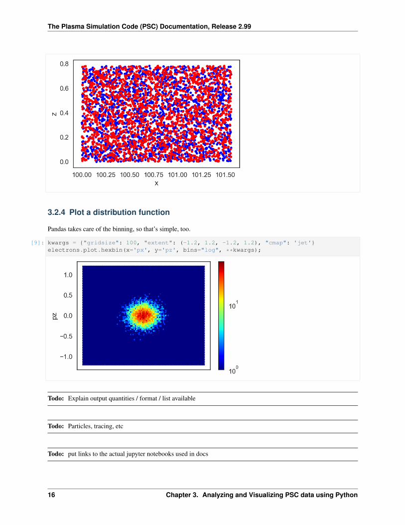
The Plasma Simulation Code (PSC) Documentation Release 299
18 Chapter 4 Visualization using Paraview
CHAPTER 5
Indices and tables
bull genindex
bull modindex
bull search
19

CHAPTER 5
Indices and tables
bull genindex
bull modindex
bull search
19