Embed Size (px)
Citation preview
American Economic Review 2013, 103(5): 1759–1796 http://dx.doi.org/10.1257/aer.103.5.1759
1759
The Political Resource Curse†
By Fernanda Brollo, Tommaso Nannicini, Roberto Perotti, and Guido Tabellini*
This paper studies the effect of additional government revenues on political corruption and on the quality of politicians, both with theory and data. The theory is based on a political agency model with career concerns and endogenous entry of candidates. The data refer to Brazil, where federal transfers to municipal governments change exogenously at given population thresholds, allowing us to implement a regression discontinuity design. The empirical evidence shows that larger transfers increase observed corruption and reduce the average education of candidates for mayor. These and other more specific empirical results are in line with the predictions of the theory. (JEL D72, D73, H77, O17, O18)
Suppose new oil is discovered in a country, or more funds are transferred to a locality from a higher level of government. Are these windfalls of resources unam-biguously beneficial to society? This is a key question in the evaluation of a variety of policies, such as intergovernmental relations, transfers to lagging regions inside a nation, and international aid to developing countries.
Until a few years ago, the only reason for a negative answer to this question was the “Dutch disease” hypothesis: a natural resource windfall, such as oil revenues, can reduce income via a market mechanism, notably an appreciation of the real exchange rate. More recently, a growing literature has pointed to further adverse effects through the political process and the interaction among interest groups, lead-ing for instance to increased rent-seeking (as in the dynamic common pool models of Tornell and Lane 1999 and Velasco 1999) or even to civil war (as in Besley and Persson 2008; Caselli and Coleman 2011; and Ross 2006).
* Brollo: Department of Economics, University of Alicante, Carretera San Vicente del Raspeig, 03690 San Vicente del Raspeig, Alicante, Spain (e-mail: [email protected]); Nannicini: Department of Economics, Bocconi University, Via Roentgen 1, 20136 Milan, Italy (e-mail: [email protected]); Perotti: Department of Economics, Bocconi University, Via Roentgen 1, 20136 Milan, Italy (e-mail: roberto.perotti@ unibocconi.it); Tabellini: Department of Economics, Bocconi University, Via Roentgen 1, 20136 Milan, Italy (e-mail: [email protected]). We gratefully acknowledge financial support by the European Research Council under grant No. 230088 and by Bocconi University (Nannicini, Perotti, and Tabellini), by the Spanish Ministry of Education and Feder Funds under project SEJ 2007-62656 and by University of Alicante (Brollo). We thank Frederico Finan, Macartan Humphreys, Guy Michaels, and seminar participants at AEA-ASSA Conference 2011, ASSET Conference 2010, Bologna University, CIFAR Meeting 2010, Econometric Society World Conference 2010, EUI, FGV-SP, IEB-Barcelona, IGIER-Bocconi, INSPER, LACEA Conference 2010, LSE, MILLS, NBER Political Economy Program Meeting 2009, Oxford University, and Wallis Conference 2009 for extremely helpful comments; Eliana La Ferrara, Alberto Chong, and Suzanne Duryea for sharing their data on the 1980 Census; Gaia Penteriani, Denise Cassia Badu Alencar, and Vitor Ugo de Oliveira for excellent research assistance.
† Go to http://dx.doi.org/10.1257/aer.103.5.1759 to visit the article page for additional materials and author disclosure statement(s).
1760 THE AMERICAN ECONOMIC REVIEW AugusT 2013
This paper identifies yet another channel of adverse effects on the function-ing of political institutions, which does not hinge on conflict between interest groups: a windfall of government revenues exacerbates the political agency problem and deteriorates the quality of political candidates. This idea has been voiced before in policy debates, for instance with reference to the Italian South (Rossi 2006), but without spelling out a precise mechanism and only on the basis of anecdotal evi-dence. Here, we show that it is supported by both theory and evidence.
The theory is based on a political agency model with career concerns and endog-enous entry of political candidates. An incumbent competes for reelection against a set of challengers, all with different political abilities and different opportunity costs of entering politics. The incumbent faces a trade-off between grabbing rents for himself versus pleasing the voters to increase the probability of reelection. Although the model has been studied before (by Persson and Tabellini 2000), we emphasize some new implications on the effects of a windfall of revenues, and we extend it to allow for endogenous entry and selection of candidates with different abilities.
The model highlights several political effects of an increase in non-tax government revenues. First, there is an effect on moral hazard: with a larger budget size, the incum-bent has more room to grab political rents without disappointing rational but imperfectly informed voters. In other words, the electoral punishment of corruption decreases with budget size, and this induces the incumbent to misbehave more frequently. Second, there is a selection effect: a larger budget induces a decline in the average ability of the pool of individuals entering politics. This is a by-product of the first result (that rents increase with budget size) and of the assumption that political rents are more valuable for political candidates of lower ability. The selection effect in turn magnifies the adverse consequences on moral hazard: an incumbent facing less able opponents can marginally grab more rents without hurting his reelection prospects. As a result, and despite the increased level of corruption, in equilibrium a windfall of government revenues also increases the reelection probability of the incumbent.
We test the main implications of our model on micro data from a sample of Brazilian municipalities. The obvious problem in testing the effects of government revenues is, as always, how to identify exogenous changes: one can think of several reasons why local government revenues might be correlated with corruption and the composition of the pool of politicians. For instance, corrupt politicians might have a comparative advantage in obtaining larger transfers from higher levels of government; or poorer areas might select lower quality politicians and, at the same time, receive more trans-fers. To address endogeneity, we exploit a key feature of federal transfers in Brazil: transfers to municipalities should change exogenously and discontinuously at given population thresholds, with all municipalities in the same state and in a given popu-lation bracket receiving the same transfers. Indeed, although there are some cases of misassignments around the population thresholds, the federal amount received by municipalities displays visible jumps at each threshold. We therefore use a (fuzzy) regression discontinuity approach—with population discontinuities as an instrument for the transfers actually received—to study the effects of a discrete change in transfers between municipalities just above or below the thresholds. Our indicators of perfor-mance refer to episodes of corruption by incumbent mayors (as measured by a random audit program on municipal budgets performed by the central government) and to the quality composition of the pool of opponents (as captured by their education).
1761Brollo et al.: the Political resource curseVol. 103 No. 5
The empirical findings accord well with the predictions of the theory. Specifically, an (exogenous) increase in federal transfers by 10 percent raises the incidence of a broad measure of corruption by 4.7 percentage points (about 6 percent with respect to the average incidence), and the incidence of a more restrictive measure— including only severe violation episodes—by 7.3 percentage points (about 16 percent). At the same time, larger transfers by 10 percent worsen the quality of the political candi-dates challenging the incumbent, decreasing the fraction of opponents with at least a college degree by 2.7 percentage points (about 6 percent). As a result, an incum-bent receiving larger transfers experiences a raise in his probability of reelection by 4 percentage points (about 7 percent).
In principle, there is more than one reason why additional non-tax revenues might induce more corruption in our data. But our model of political agency has two more specific predictions, which can help discriminate between our explana-tion and others. First, the central mechanism driving the theoretical results revolves around the following implication: an incumbent who receives a larger budget faces a weaker electoral punishment for corruption. To test this prediction, we combine our regression discontinuity design with the identification strategy used by Ferraz and Finan (2008), and compare the electoral punishment of disclosed corruption just above and below the population thresholds. This evidence suggests that the electoral punishment is weaker just above the thresholds, where transfers are larger, as predicted by the theory.
The second specific prediction of the theory is an interaction between the indi-vidual features of politicians and the detrimental effect of windfall resources: higher transfers increase corruption by more if the opponents have lower educational attain-ments. This prediction too is borne out by the data. In addition, the Brazilian institu-tions and data reject alternative mechanical or political explanations of our findings. In particular, there is no evidence that larger transfers have an impact on the political orientation of the mayor, or on the amount and sources of campaign resources that the mayor can mobilize.
At the theoretical level, our paper combines three separate strands of literature, besides the career concerns model discussed by Persson and Tabellini (2000). The first is the literature on windfall resources and rent-seeking mentioned above. Our closest antecedent here is Robinson, Torvik, and Verdier (2006), who use a par-tisan model with patronage to study the optimal extraction of resources and the optimal patronage by a government facing reelection. A second strand of literature studies the selection of politicians, and how different institutions affect the pool of elected officials and candidates (Besley 2004; Caselli and Morelli 2004; Besley and Smart 2007; Mattozzi and Merlo 2008; Galasso and Nannicini 2011). A third, older strand of literature studies the allocation of talents in economies characterized by different incentives to different types of talents (Baumol 1990; Murphy, Shleifer, and Vishny 1991).
With regard to the evidence, to our knowledge, we are the first to estimate the effect of central transfers on political corruption and on the quality of politicians at the local level. Litschig (2008a) is somehow our closest antecedent: he uses the same Brazilian dataset on federal transfers but applies a sharp (instead of fuzzy) regres-sion discontinuity design, because the data he uses are from the 1980s, when epi-sodes of misassignments around the thresholds were not yet detected. He shows that
1762 THE AMERICAN ECONOMIC REVIEW AugusT 2013
higher federal transfers increase municipal spending on public schools and improve literacy rates. Although he does not talk about corruption, his findings are consistent with ours. Litschig and Morrison (2009) also use a (sharp) discontinuity design for the municipal term 1984–1988 and estimate the impact of federal transfers on the reelection probability of the incumbent party in mayoral elections, detecting a positive and significant effect. Using a tailored household survey, Vicente (2010) shows that the discovery of oil in the island of São Tomé and Principe was associ-ated with a significant rise in perceived corruption, relative to the control island of Capo Verde. Caselli and Michaels (2011) show that oil discoveries in Brazilian municipalities have a positive impact on public good spending, but little or no effect on the quality of public good provision. They also provide indirect evidence that this might be due to rent-seeking. Ferraz and Finan (2008, 2011) use instead the dataset on randomized audits to study, respectively, the effect of corruption disclosure on the election outcome and the effect of electoral accountability on political corrup-tion: they find that mayors disclosed as corrupt have a lower reelection probability, and that municipalities where mayors can be reelected experience less corruption. Brollo (2011) uses similar data and finds that corrupt municipalities are also pun-ished by a reduction in discretionary transfers for infrastructures.1
The outline of the paper is as follows. Section I presents the theory and derives its empirical implications. Section II discusses the relevant Brazilian institutions and describes the data. Section III illustrates the econometric strategy. Section IV presents the estimation results. We conclude with Section V. Theoretical derivations, validity tests, and further robustness checks are collected in the online Appendix.
I. Theory
This section lays out a political agency model based on “career concerns” of poli-ticians. Although a simpler version of this model has been studied before by Persson and Tabellini (2000), its detailed implications provide a useful road map for the empirical analysis. More importantly, Section IC extends the framework of Persson and Tabellini (2000) to allow for endogenous entry into politics. This yields new theoretical results and additional predictions.
A. A Career Concerns Model
Although the model can be formulated with an infinite horizon, for simplicity we assume only two periods. Throughout, we refer to the politician in office as the incumbent mayor. In the first period (t = 1) an incumbent mayor sets policy for that period. Then elections are held, and the elected mayor sets policy once more for a second (t = 2) and last period. In both periods, a budget of fixed size τ can be
1 Recent papers by Litschig and Zamboni (2012) and Brollo and Troiano (2012) also use corruption data to evaluate the impact of judicial presence or gender differences in politics, respectively. Our paper is also related to a recent literature on political selection, which has focused on the impact of monetary and non-monetary incentives on the decision of citizens to run for an elective office (Diermeier, Keane, and Merlo 2005; Messner and Polborn 2004; Gagliarducci, Nannicini, and Naticchioni 2010; Gagliarducci and Nannicini 2013; Ferraz and Finan 2009). So far, however, this literature has not investigated how the quality of political candidates is affected by the size of the government budget.
1763Brollo et al.: the Political resource curseVol. 103 No. 5
allocated to two alternative uses: rents r t that only benefit the mayor; and a public good g t that only benefits the voters. The cost of providing the public good depends on the identity of the mayor, and more competent mayors can provide the same public good (expressed in terms of voters’ utility) at a lower resource cost. Specifically, the government budget constraint is
(1) g t = θ(τ − r t ),
where θ reflects an individual’s competence in providing the public good if in office; a higher value of θ corresponds to a lower cost of providing the public good, and hence a more competent mayor.
We assume political competence to be a random but permanent feature of an individual. Specifically, θ is a random variable uniformly distributed with density ξ and a known mean. The realization of θ is drawn from two alternative distribu-tions, with the same density but different means, depending on the individual’s type. Specifically, for an individual of type J the mean of θ is 1 + σ J , where J = H, L, and σ H = σ = − σ L , with 1 > σ > 0 a known parameter. Thus, on average types H are more competent. But, in specific instances, it might very well be that an individual of type L is more competent than one of type H.
In keeping with the career concerns model, we assume that the realization of θ becomes known to each individual, and also to voters if that individual is elected to office, only at the end of period 1. The mayor’s and his opponent’s types are known beforehand to everyone, however. At the time of elections, voters also observe their own utility (i.e., the public good g 1 ), but do not observe political rents. All the parameters of the model are known to the voters.
This formulation captures two important features of political agency conflicts. On the one hand, as in the standard career concerns model, the voters’ imperfect information about the incumbent’s true competence creates an incentive for the incumbent to please the voters through public good provision, so as to appear competent. On the other hand, not all politicians are ex ante identical: voters know something about political candi-dates, besides what is learned by observing policy outcomes. Throughout this section we refer to the mayor’s type J as simply high or low quality, but more generally J stands for any observable variable (other than policy outcomes) that enables voters to predict the mayor’s performance if elected. In the empirical section, we measure J by the politi-cians’ education. For now, the politician’s type is exogenous. In Section IB, we make it endogenous by analyzing the entry decision of candidates.
In line with the institutions in Brazil, we assume that rent-seeking (corruption) by the mayor is discouraged by an audit technology. Specifically, with probability d( r t ) = q r t a mayor who grabbed political rents r t is caught and suffers utility loss of λ J , where λ H > λ L > 0.2 Thus, the loss of utility for a high quality mayor who is caught cheating is harsher. This assumption plays a crucial role below, where we analyze the entry of political candidates, and it is further discussed there. It is meant to capture the idea that a highly educated politician has more valuable opportunities
2 As explained in footnote 3, the results of interest would be reinforced if we assumed that the probability of being caught depends on the fraction of the budget devoted to rents (rather than on the absolute amount).
1764 THE AMERICAN ECONOMIC REVIEW AugusT 2013
outside of politics. Hence, his reputation cost of being caught in an act of corruption is higher than for someone with lower opportunity costs from being in politics.
As standard in the literature on political agency, politicians care about political rents (net of the expected penalty), and enjoy other exogenous benefits from being in office (ego rents), summarized by the exogenous variable R. Thus, the expected utility of a mayor of type J who is in office in periods 2 and 1, respectively, is
(2) V 2 J = α J r 2 + R,
(3) V 1 J = α J r 1 + R + p J V 2 J ,
where α J = 1 − λ J q denotes the expected value of political rents for type J, and p J is the probability of being reelected, as perceived by the incumbent in period 1, when setting the optimal rent r 1 . We assume that λ J < 1, so that α J > 0 for all J. Voters only care about the public good, hence their preferences in each period are W t = g t . Finally, we assume that rents cannot exceed a given upper bound that depends on the size of the budget, namely: r t ≤ ψτ ≡ _ r .
The timing of events is as follows.• Atthestartofperiod1,theincumbentsetsr 1 . He knows his own type, but he
does not yet know the actual realization of his competence, θ, nor the identity of his future opponent. Specifically, the incumbent expects his opponent to be of type L with probability π, and of type H with probability 1 − π, where for now 1 > π > 0 is given, but will be endogenized later (the assumption that the incumbent does not yet know his opponent’s identity is made to simplify notation and with no loss of generality). For later use, we denote the expected quality of the opponent as: σ = π σ H + (1 − π) σ L .
• Theidentityoftheopponentisrevealedandhistype H or L (but not the actual realization of his competence θ) becomes known to all.
• Electionsareheld.Whenvoting,votersobserveg 1 , but not r 1 . They also know the incumbent’s as well as the opponent’s type. After the elections, the audit takes place and the penalty is paid (if cheating is detected).
• In period2 the elected mayor sets r 2 , and then a second and final audit takes place.
B. Equilibrium Rents
Here we state the main properties of the equilibrium, giving particular emphasis to the predictions that are tested in the empirical analysis below. Complete derivations are in the online Appendix. We confine attention to period 1, which is more interesting.
PREDICTION 1: The electoral punishment for rents, ∂ p J _ ∂ r 1 , becomes smaller in abso-
lute value as τ rises. As a result, rents are an increasing function of τ, ∂ r 1 J _ ∂ τ > 0.
Intuitively, if the budget size increases, there is more room to grab political rents without disappointing the voters. This in turn reflects how voters form their inferences: as the budget grows in size, a dollar stolen has a smaller impact on
1765Brollo et al.: the Political resource curseVol. 103 No. 5
voters’ inferences about the incumbent’s unobserved ability. As a consequence, a larger budget weakens the incentive to please the voters, and rents increase with τ.3
Prediction 2: Rents are a decreasing function of the quality of the incumbent,
r 1 H < r 1 L , and of the expected quality of the opponent: ∂ r 1 J _ ∂ σ < 0.
the first part follows from the assumption that high quality incumbents face a larger penalty if they are caught cheating. the second part is more subtle. intuitively, an opponent of high quality entails a higher competence threshold to reappoint the incumbent, and reduces the reelection probability for any level of rents consistent with voters’ expectations. At this higher reelection threshold, the probability of win-ning the election is more sensitive to political rents. this sharpens the incumbent’s incentive to please voters, and as a result equilibrium rents fall.
Prediction 3: The effect of budget size on rents is smaller the higher is the
expected quality of the opponent: ∂ 2 r 1 J
_ ∂ τ∂ σ < 0.
this interaction effect between τ and σ reflects the same forces that account for the previous two predictions. As shown in the online Appendix, when the budget size increases by one dollar, the incumbent grabs the extra dollar less a quantity which is a function of the electoral threshold times the value of reelection; hence, a higher expected quality of the opponent (a higher electoral threshold) reduces the share of the extra dollar of budget grabbed by the incumbent. not only does a larger budget increase political rents (Prediction 1), but it also does so to a larger extent if the oppo-nent is more likely to be of low quality (if σ is small or, equivalently, if π is large).
c. The Quality of Political Candidates
the model emphasizes the role of elections in selecting the more competent candidate, and the implied effects on the incumbent’s incentives. But the pool of candidates was taken as exogenous, neglecting how individuals respond to incen-tives in deciding whether or not to stand as a political candidate. in this subsection we address this issue, and allow the proportion of high and low quality types in the pool of candidates to be determined endogenously in equilibrium. For this we need additional assumptions.
Let 2N be the overall population, with N a discrete large number. in the population there are two groups of individuals indexed by J = H, L, with each group of size N. All the assumptions outlined above continue to hold. in particular, if an individual in group J holds office, his competence is drawn from a uniform distribution with mean 1 + σ J .
3 note that, almost by assumption, period 2 rents are also an increasing function of budget size. this dampens the effect of budget size on period 1 rents, because it raises the value of reelection, but (at an interior optimum) it is not enough to offset the effect of τ on r 1 J that operates through the term ∂ p J /∂ r 1 . it is also easy to see that Proposition 1 would be strengthened if we assumed that the probability of being caught is increasing in the fraction of the budget devoted to rents (d( r t ) = q r t /τ), rather than in the absolute amount of rents (d( r t ) = q r t ). intuitively, under the alternative assumption, a larger budget would reduce the probability of detection, inducing the incumbent mayor to grab even more rents.
1766 THE AMERICAN ECONOMIC REVIEW AugusT 2013
Within each group, individuals differ by the opportunity cost of entering into politics: individual i in group J has opportunity cost β i y J , for i = 1, 2, … , N. To simplify the algebra, we assume that β i = i. Thus, for the first individual in group J the opportunity cost of being into politics is y J , for the second individual it is 2 y J , and so on until the last one has opportunity cost N y J . Throughout we assume that y H > y L > 0. Thus, consistently with the previous political interpretation, high quality individuals (J = H) have a higher expected competence if they become mayor and also have a higher opportunity cost of being in politics. The parameter β i instead is unrelated to political competence, so that the relationship between politi-cal competence and the opportunity cost of being in politics is not one-for-one. This formulation captures the idea that political competence is related to features, such as education or sheer talent, that also make an individual more productive in the private sector. But the decision to enter politics also reflects other considerations besides income, and the skills needed to be a successful politician do not coincide with those that yield high income or success in other professions. The positive cor-relation between market skills (outside opportunities) and political competence is common in the models on political selection, such as Caselli and Morelli (2004) and Besley (2004).
At the start of period 1, individuals decide whether or not to enter politics. Entering politics means that, with some probability, the individual is selected to run as the single opponent to the incumbent in the elections that are held at the end of period 1. If he is then elected into office, given that he is of type J, he gets an expected util-ity of V 2 J
, as defined above. A political candidate who loses the election or is not selected to be the opponent, gets zero utility.
In other words, entering politics is equivalent to entering the pool of candidates from which the opponent is selected. We do not model how parties select a hierarchy of political candidates, and simply assume that all individuals in the pool of candi-dates have the same probability to be selected as the opponent, irrespective of their types J and i. Specifically, suppose that n J individuals from group J have decided to enter politics, J = H, L. Then the pool of candidates has size n = n H + n L , and each one of them has probability 1 _ n to become the single opponent who will challenge the incumbent. This captures the notion that not all politicians get a chance to become serious political candidates for mayor.
To simplify the notation and with no loss of generality, we also assume that, when deciding whether or not to enter politics, individuals know their own type but do not know yet the identity of the incumbent and assign equal probabilities to the event that the incumbent is of type H or L. Let p ∗J denote the expected prob-ability that an opponent of type J wins the election (with a slight abuse of notation here we use the symbol J to denote the opponent—rather than the incumbent—type). Under the assumptions stated above, if individual i in group J stays out of politics, then he gets utility i y J . If he enters politics, then with probability 1 _ n he is selected to become the opponent, and with probability p ∗J he wins the election and gains office in period 2, getting expected utility of V 2 J
. With this notation, the ith individual in group J prefers to enter politics if
(4) i y J ≤ p ∗J
_ n V 2 J .
1767Brollo et al.: the Political resource curseVol. 103 No. 5
We now briefly discuss how the composition of the pool of opponents depends on budget size. The online Appendix proves the following.
PREDICTION 4: The fraction of low quality types in the pool of opponents is an increasing function of budget size: ∂ π _ ∂ τ > 0.
Intuitively, because the value of rents is higher for the low quality mayors, a larger budget increases the value of office by more for the low quality than for the high quality candidates. Hence, at the margin more low quality candidates enter the pool of opponents.
This result reflects two assumptions in the model. First, the penalty if caught is higher for a high quality type ( λ H > λ L ), which implies that rents are less valuable for a high quality type ( α H < α L ). If this assumption were reversed, the empiri-cal implication too would be the opposite. Thus, although we find our assumption a priori plausible, it can be tested with the model (see also Prediction 2 above, which is crucially linked to the same assumption). Second, the model focuses on the decision of individual candidates to enter politics, but it has nothing to say on how parties select amongst alternative candidates (since we assumed that all prospective candidates have the same probability 1/n of running as the opponent). Without a richer model of intra-party politics it is difficult to assess how restrictive this omission is.
The model also predicts how budget size affects the probability of reelection.
PREDICTION 5: The probability of reelection of an incumbent of type J is an
increasing function of budget size: d p ∗J
_ dτ > 0.
This follows directly from the previous result: as the budget size increases, more low quality individuals are drawn into the pool of opponents. Thus, despite grab-bing more rents, in equilibrium the incumbent is more likely to be reappointed. This result reflects voters’ rationality. Voters realize that equilibrium rents have increased with a larger budget, but they only care about the competence of future mayors. Hence, as the pool of opponents deteriorates in quality, voters become less demand-ing and apply a lower quality threshold for reelecting the incumbent. As a result, the incumbents’ chances of winning go up.
Predictions 4 and 5 highlight an important implication of the analysis: a wind-fall of revenues is harmful not only because it tempts public officials into more corruption, but also because over time it leads to a deterioration of the quality of elected officials. This result is related to those obtained by Murphy, Shleifer, and Vishny (1991). But whereas they consider the allocation of talent between produc-tive and rent-seeking activities in the private sector, here we highlight the implica-tions of windfall revenues for the selection of talents into public office.
Finally, putting it all together, we can determine the total effect of budget size, taking into account also its effects on the quality of the opponents. It is easy to see that Prediction 1 is strengthened once the composition of opponents is endogenous.
1768 THE AMERICAN ECONOMIC REVIEW AugusT 2013
PREDICTION 6: The overall effect of budget size on rents is positive: dr 1 J _ dτ = ∂r 1 J
_ ∂ τ | σ
+ ∂ r 1 J _ ∂ σ | τ ∂ σ _ ∂ τ > 0.
The result follows because both terms in the total derivative of r 1 J with respect to τ
are positive; the first term by Prediction 1, the second term because, from Prediction 4, ∂ σ /∂τ < 0. Prediction 6 summarizes the two main forces at work in this model. The first is the positive effect of τ on rents holding constant the composition of the pool of opponents, i.e., holding constant π; this is the moral hazard effect. The second is the positive effect of τ on rents due to the response of the composition of the pool of opponents; this is the interaction between the moral hazard and the opponents’ selection effect.
D. Discussion
The predictions concerning the political moral hazard effects of a windfall of government revenues are very robust, since they would also follow from other mod-els of political agency, such as that of Barro (1973) and Ferejohn (1986), reviewed in Persson and Tabellini (2000). In that framework, political rents stem from con-tractual incompleteness, rather than incomplete information. Once in office, the incumbent can appropriate political rents, and the only weapon available to voters is the threat of throwing him out of office at the next election if he misbehaves too much. As the budget size increases, so does the temptation to grab rents, and even fully informed voters have to accept a higher level of political abuse. Thus, this framework too yields the prediction that a windfall of government resources aggra-vates moral hazard, because the electoral punishment of corruption is weakened as budget size increases. In the career concerns model, this happens through voters’ inferences: voters find it harder to detect misbehavior. In the political accountability framework of Barro and Ferejohn, this happens because a larger budget exacerbates the distortion due to contractual incompleteness.
How robust are the results on the selection of political candidates? The account-ability model of Barro and Ferejohn does not lend itself to have candidates of dif-ferent qualities, so here there is no alternative theoretical benchmark with which to address this question. Nevertheless, as discussed above, the mechanism behind the adverse effects of budget size on the quality of political candidates rests on plausible features of the model.
The remainder of the paper tests these predictions on Brazilian municipal data. Specifically, we ask whether larger federal transfers are associated with: more fre-quent episodes of political corruption by the mayor (Predictions 1 and 6), particu-larly if the opponent is of low quality (Prediction 3); a lower observed quality of the pool of political opponents in the elections for mayor (Prediction 4); and more frequent reelection of the incumbent mayor (Prediction 5). To shed light on the mechanisms that lead to more corruption, we also test whether larger transfers entail a weaker electoral punishment of corruption (the first part of Prediction 1). We can also indirectly assess one additional implication, namely that episodes of political corruption are more frequent when the incumbent and the opponents are of lower
1769Brollo et al.: the Political resource curseVol. 103 No. 5
quality (Prediction 2). However, for the empirical test of this last implication—unlike for the others—we must rely on descriptive rather than quasi-experimental evidence for the reasons discussed in Section III.
II. Institutions and Data
This section describes the institutional framework and the data we use in the empirical analysis. The main variables of interest refer to federal transfers to munic-ipal governments (τ in the model), corruption ( r t and q r t ), and the observed quality of political candidates (their type J ). The empirical counterpart of each of these variables is described in a separate subsection below.
A. Federal Transfers to Municipal Governments
Institutional Framework.—Brazilian municipal governments are managed by an elected mayor (Prefeito) and an elected city council (Camara dos Vereadores). Following the 1988 Constitution, mayors are directly elected by voters with a first-past-the-post system in cities below 200,000 eligible voters, and with a runoff sys-tem in cities above. Since the 2000 elections, the term limit for mayors has been extended from one to two terms. The municipal term lasts four years, and elections are usually held in October (oath of office taking place in January of the following year). A clear separation is maintained between the mayor, who holds executive powers, and the city council, which holds legislative powers. The mayor is the cru-cial political player when it comes to shape the budget and implement expenditure programs. The city council has the power to impeach the mayor, but only for serious reasons and based on a qualified majority of at least 2/3. If an impeachment vote is successful, the vice mayor shall take office until the end of the term.
Municipal governments are in charge of a relevant share of the provision of public goods and services related to education, health, and infrastructure projects. Most of the municipal resources are intergovernmental transfers from either the federal or the state government. For municipalities with less than 50,000 inhabitants—those included in our sample for the reasons discussed below—local taxes represent only 6 percent of total revenues. The single most important source of municipal revenues (40 percent) is the Fundo de Participação dos Municipios (FPM), con-sisting of automatic federal transfers established by the Federal Constitution of Brazil (Art. 159 Ib). FPM transfers amount to 75 percent of all federal transfers and, according to the rules that regulate the allocation of these funds, municipal governments must spend 15 percent of them for education and 15 percent for health care, while the remainder is unrestricted. Our study focuses on this type of transfers, both for their relevance and because their allocation depends on population size in a discontinuous fashion that is crucial for our identification strategy (see Section III).
According to the FPM allocation mechanism, municipalities are divided into pop-ulation brackets that determine the coefficients used to share total state resources earmarked for the FPM, with smaller population brackets corresponding to lower coefficients. Since each state receives a different share of the total resources ear-marked for FPM, two municipalities in the same population bracket receive iden-tical transfers only if they are located in the same state. More precisely, define
1770 THE AMERICAN ECONOMIC REVIEW AugusT 2013
FP M i k as the amount of FPM transfers received by municipality i in the state k. The revenue-sharing mechanism is
FP M i k = FP M k λ i _ ∑ i∈k
λ i
,
where FP M k is the amount of resources allocated to state k and λ i is the FPM coef-ficient of municipality i based on its population size.4
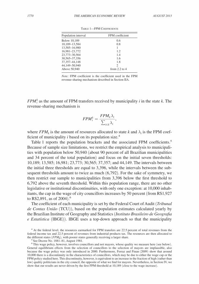
Table 1 reports the population brackets and the associated FPM coefficients.5 Because of sample size limitations, we restrict the empirical analysis to municipali-ties with population below 50,940 (about 90 percent of all Brazilian municipalities and 34 percent of the total population) and focus on the initial seven thresholds: 10,189; 13,585; 16,981; 23,773; 30,565; 37,357; and 44,149. The intervals between the initial three thresholds are equal to 3,396, while the intervals between the sub-sequent thresholds amount to twice as much (6,792). For the sake of symmetry, we then restrict our sample to municipalities from 3,396 below the first threshold to 6,792 above the seventh threshold. Within this population range, there are no other legislative or institutional discontinuities, with only one exception: at 10,000 inhab-itants, the cap in the wage of city councillors increases by 50 percent (from R$1,927 to R$2,891, as of 2004).6
The coefficient of each municipality is set by the Federal Court of Audit (Tribunal de Contas União (TCU)), based on the population estimates calculated yearly by the Brazilian Institute of Geography and Statistics (Instituto Brasileiro de Geografia e Estatística (IBGE)). IBGE uses a top-down approach so that the municipality
4 At the federal level, the resources earmarked for FPM transfers are 22.5 percent of total revenues from the federal income tax and 22.5 percent of revenues from industrial products tax. The resources are then allocated to the different states (FP M k ), with poorer states generally receiving a larger share.
5 See Decree No. 1881–81, August 1981.6 This wage policy, however, involves councillors and not mayors, whose quality we measure here (see below).
General equilibrium effects from the selection of councillors to the selection of mayors are implausible, also because the wage policy was only introduced in 2000. Furthermore, Ferraz and Finan (2009) show that around 10,000 there is a discontinuity in the characteristics of councillors, which may be due to either the wage cap or the FPM policy studied here. This discontinuity, however, is equivalent to an increase in the fraction of high (rather than low) quality politicians in the city council, the opposite of what we find for mayors. Nevertheless, in Section IV, we show that our results are never driven by the first FPM threshold at 10,189 (close to the wage increase).
Table 1—FPM Coefficients
Population interval FPM coefficient
Below 10,189 0.610,189–13,584 0.813,585–16,980 116,981–23,772 1.223,773–30,564 1.430,565–37,356 1.637,357–44,148 1.844,149–50,940 2Above 50,940 from 2.2 to 4
Note: FPM coefficient is the coefficient used in the FPM revenue-sharing mechanism described in Section IIA.
1771Brollo et al.: the Political resource curseVol. 103 No. 5
estimates are consistent with the state estimates, which in turn are consistent with the estimated population of the whole country, based on birth, mortality, and immi-gration rates between subsequent censuses. In the online Appendix, we describe the procedure followed by IBGE to calculate the estimates.
As further discussed below, population estimates from IBGE in a given year, how-ever, do not perfectly predict the FPM transfers each municipality receives in the following year. There may be various reasons for that. During the 1990s, several municipalities split and this reduced the population size of pre-existing munici-palities. As a result, a municipality that had lost part of its population should have had its coefficient reduced according to the new population. However, several law amendments froze the FPM coefficients and this practice generated major distor-tions. In order to avoid these distortions, the federal government established that by 2008 all municipalities should be framed in FPM coefficients corresponding to their actual population estimate. To avoid shocks in the finance of the involved municipalities, however, the law established a transition period to the new regime, so that in the period 2001–2008 some municipalities still received FPM transfers that were not consistent with their population. Furthermore, the FPM allocation procedure is not audited, and opportunistic manipulation of the data around the thresholds cannot be ruled out. The population figures used by TCU and the associ-ated coefficients are published in the Diário Oficial da União. For some years, we compared population estimates from IBGE and those used by TCU, and they do not perfectly coincide. Although there are several possible explanations for this, oppor-tunistic manipulation of the TCU figures is one of them.7 While we allow the TCU data to be manipulated strategically, throughout we maintain the assumption of no manipulation in the IBGE figures, and we formally test this assumption in the online Appendix by means of different empirical strategies.
Data on Transfers.—Our data cover two mayoral terms: January 2001–December 2004 and January 2005–December 2008. We measure two key variables of the FPM revenue-sharing mechanism: the amount of federal transfers and the IBGE population estimates.
Data on FPM transfers received by each municipality are available from the website of the Brazilian National Treasury (Tesouro Nacional). The variable we use in the empirical analysis is the average amount of transfers in the first three years of each term (in real values), therefore excluding electoral years.8 In the model, the parameter τ refers to both actual and expected transfers. Actual transfers influence corruption in the same period. Expected future transfers influence the composition of the pool of opponents. Here, we use average transfers in the first three years of the legislature as a measure of both actual and expected transfers. Thus, in the analysis concerning the quality of the opponents, current average transfers stand as a proxy for the future transfers expected by mayoral candidates in the next term. The averag-ing across years within the same term is also meant to minimize measurement error.
7 Litschig (2008b) detects some evidence of manipulative sorting around the FPM thresholds in the TCU popula-tion figures for the years 1989 and 1991.
8 We cannot use 2008 (the electoral year at the end of term 2005–2008) because the IBGE population estimates for 2007 are not available; we therefore also exclude 2004 (the electoral year at the end of term 2001–2004) for consistency. Estimation results are not sensitive to this choice.
1772 THE AMERICAN ECONOMIC REVIEW AugusT 2013
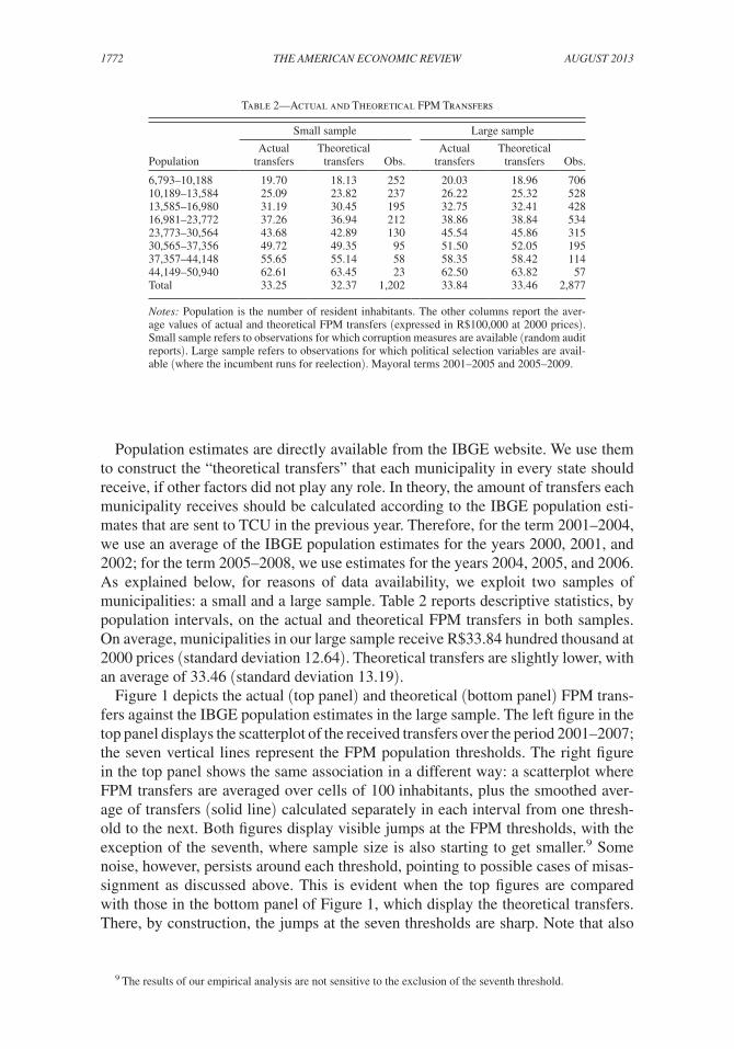
Population estimates are directly available from the IBGE website. We use them to construct the “theoretical transfers” that each municipality in every state should receive, if other factors did not play any role. In theory, the amount of transfers each municipality receives should be calculated according to the IBGE population esti-mates that are sent to TCU in the previous year. Therefore, for the term 2001–2004, we use an average of the IBGE population estimates for the years 2000, 2001, and 2002; for the term 2005–2008, we use estimates for the years 2004, 2005, and 2006. As explained below, for reasons of data availability, we exploit two samples of municipalities: a small and a large sample. Table 2 reports descriptive statistics, by population intervals, on the actual and theoretical FPM transfers in both samples. On average, municipalities in our large sample receive R$33.84 hundred thousand at 2000 prices (standard deviation 12.64). Theoretical transfers are slightly lower, with an average of 33.46 (standard deviation 13.19).
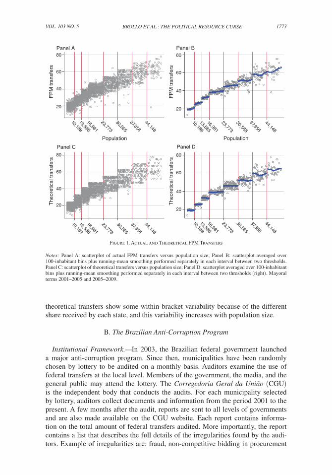
Figure 1 depicts the actual (top panel) and theoretical (bottom panel) FPM trans-fers against the IBGE population estimates in the large sample. The left figure in the top panel displays the scatterplot of the received transfers over the period 2001–2007; the seven vertical lines represent the FPM population thresholds. The right figure in the top panel shows the same association in a different way: a scatterplot where FPM transfers are averaged over cells of 100 inhabitants, plus the smoothed aver-age of transfers (solid line) calculated separately in each interval from one thresh-old to the next. Both figures display visible jumps at the FPM thresholds, with the exception of the seventh, where sample size is also starting to get smaller.9 Some noise, however, persists around each threshold, pointing to possible cases of misas-signment as discussed above. This is evident when the top figures are compared with those in the bottom panel of Figure 1, which display the theoretical transfers. There, by construction, the jumps at the seven thresholds are sharp. Note that also
9 The results of our empirical analysis are not sensitive to the exclusion of the seventh threshold.
Table 2—Actual and Theoretical FPM Transfers
Small sample Large sample
Actual Theoretical Actual TheoreticalPopulation transfers transfers Obs. transfers transfers Obs.
6,793–10,188 19.70 18.13 252 20.03 18.96 70610,189–13,584 25.09 23.82 237 26.22 25.32 52813,585–16,980 31.19 30.45 195 32.75 32.41 42816,981–23,772 37.26 36.94 212 38.86 38.84 53423,773–30,564 43.68 42.89 130 45.54 45.86 31530,565–37,356 49.72 49.35 95 51.50 52.05 19537,357–44,148 55.65 55.14 58 58.35 58.42 11444,149–50,940 62.61 63.45 23 62.50 63.82 57Total 33.25 32.37 1,202 33.84 33.46 2,877
Notes: Population is the number of resident inhabitants. The other columns report the aver-age values of actual and theoretical FPM transfers (expressed in R$100,000 at 2000 prices). Small sample refers to observations for which corruption measures are available (random audit reports). Large sample refers to observations for which political selection variables are avail-able (where the incumbent runs for reelection). Mayoral terms 2001–2005 and 2005–2009.
1773Brollo et al.: the Political resource curseVol. 103 No. 5
theoretical transfers show some within-bracket variability because of the different share received by each state, and this variability increases with population size.
B. The Brazilian Anti-Corruption Program
Institutional Framework.—In 2003, the Brazilian federal government launched a major anti-corruption program. Since then, municipalities have been randomly chosen by lottery to be audited on a monthly basis. Auditors examine the use of federal transfers at the local level. Members of the government, the media, and the general public may attend the lottery. The Corregedoria Geral da União (CGU) is the independent body that conducts the audits. For each municipality selected by lottery, auditors collect documents and information from the period 2001 to the present. A few months after the audit, reports are sent to all levels of governments and are also made available on the CGU website. Each report contains informa-tion on the total amount of federal transfers audited. More importantly, the report contains a list that describes the full details of the irregularities found by the audi-tors. Example of irregularities are: fraud, non-competitive bidding in procurement
Figure 1. Actual and Theoretical FPM Transfers
Notes: Panel A: scatterplot of actual FPM transfers versus population size; Panel B: scatterplot averaged over 100-inhabitant bins plus running-mean smoothing performed separately in each interval between two thresholds. Panel C: scatterplot of theoretical transfers versus population size; Panel D: scatterplot averaged over 100-inhabitant bins plus running-mean smoothing performed separately in each interval between two thresholds (right). Mayoral terms 2001–2005 and 2005–2009.
20
40
60
80F
PM
tran
sfer
s
10,189
13,585
16,981
23,773
37,356
44,148
Population Population
The
oret
ical
tran
sfer
s
10,189
13,585
16,981
23,773
30,565
37,356
44,148
Population
10,189
13,585
16,981
23,773
30,565
37,356
44,148
Population
20
40
60
80
20
40
60
80
FP
M tr
ansf
ers
The
oret
ical
tran
sfer
s
20
40
60
80
30,565
10,189
13,585
16,981
23,773
30,565
37,356
44,148
Panel A Panel B
Panel C Panel D
1774 THE AMERICAN ECONOMIC REVIEW AugusT 2013
contracts, over-invoicing, diversion of funds, lack of completeness, non-utilization of the funds, undocumented expenses, as well as others.
Between 2003 and 2004, in each lottery, 50 municipalities were randomly selected to be audited. Since 2004, 60 municipalities have been selected in each lottery. To date, the total number of audited municipalities is over 1,500. The program thus provides a valuable source of information on budget irregularities and corruption episodes in municipal governments.
The management of the audited funds falls under the responsibility of the exec-utive branch run by the mayor, who is thus directly or indirectly linked to most of the disclosed violations. The city council is not involved in the management of the programs, although it should act as an oversight authority. In recent years, also following the success and the publicity of the federal anti-corruption pro-gram, city councillors strengthened their own role to check on the executive’s actions; for instance, they created independent anti-corruption commissions or, in ill-famed cases, they voted to impeach the mayor because of alleged corrup-tion charges.
Most of the audits concern projects or public works financed by specific fed-eral transfers other than the FPM transfers, although some projects financed or cofinanced by the municipality unconstrained resources (therefore including FPM transfers) are also audited. Thus, in the analysis below, we ask how an exogenous increase in FPM transfers around the population thresholds affects corruption in the use of all sources of municipal revenues. Since 70 percent of FPM transfers are unrestricted and given that FPM transfers account for the largest fraction of municipal revenues, this question corresponds to a test of Predictions 1 and 6 in the model (how rents react to a change in overall budget size τ). Specifically, the theory predicts that, as FPM transfers increase, municipal governments feel less restrained in pleasing the voters and engage in more abuses of all kinds, and not just abuses concerning the FPM transfers.
We now describe in more detail how we classify each occurrence in the audit reports, in the spirit of Ferraz and Finan (2008, 2011).
Data on Corruption.—Because of sample size limitations in the audited local gov-ernments, we restrict the sample to municipalities with less than 50,940 inhabitants, corresponding to the first seven FPM thresholds (see Table 1). In the two mayoral terms of our analysis, 1,202 municipalities for which we have non-missing data in the other relevant variables were randomly selected through the first 29 lotteries of the Brazilian anti-corruption program. The bad administration and corruption occurrences reported in the audit reports are thus related to the municipal adminis-tration that was in power during the two terms in our sample (802 municipalities in 2001–2004 and 400 municipalities in 2005–2008).
Many types of irregularities are detected by the audit reports. Illegal procure-ment practices, diversion of funds, over-invoicing of goods and services, and fraud are the most common occurrences. We introduce two definitions of corruption: broad corruption, which includes irregularities that could also be interpreted as bad administration rather than as overt corruption; and narrow corruption, which only includes severe irregularities that are also more likely to be visible to voters. For both definitions, we construct a binary variable (whether any irregularity was found
1775Brollo et al.: the Political resource curseVol. 103 No. 5
or not) and a continuous indicator, namely the ratio between the total amount of funds involved in the detected violation and the total amount audited. This normal-ized indicator—which we call broad fraction of the amount and narrow fraction of the amount for general and severe violations, respectively—is only available for 1,140 of the 1,202 municipalities in the small sample.10 As a robustness check, we also consider an additional measure for each definition of corruption, namely the number of violation episodes detected in the audit reports. The results for these dis-crete measures are similar to those for the fractions of the amount discussed below and are reported in the online Appendix.
The definition of broad corruption includes the following categories of violation episodes: (i) “illegal procurement practices,” occurring when any of these episodes are reported: (a) competition has been limited, for example, when associates of the mayor’s family or friends receive non-public information related to the value of the project, (b) manipulation of the bid value, (c) an irregular firm wins the bid process, (d) the minimum number of bids is not attained, or (e) the required procure-ment procedure is not executed; (ii) “fraud;” (iii) “favoritism” in the good receipt; (iv) “over-invoicing,” occurring when there is evidence that public goods or ser-vices are purchased for a value above the market price; (v) “diversion of funds;” and (vi) “paid but not proven,” occurring when expenses are not proven. In the online Appendix, we report examples of each category. The definition of narrow corruption includes the following irregularities: (i) severe illegal procurement prac-tices; (ii) fraud; (iii) favoritism; and (iv) over-invoicing. In our opinion, many of the irregularities regarding the two categories “diversion of funds” and “paid but not proven” do not necessarily imply corruption (see again the online Appendix for relevant examples). Also some illegal procurement practices might result more from bad administration than from outright corruption: therefore, narrow corruption includes these episodes only if they resulted in severe violations, such as favoring one specific firm or manipulating the bid value.
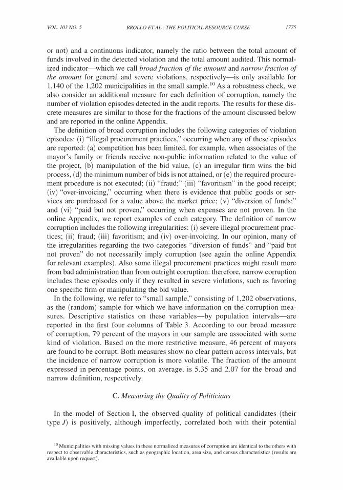
In the following, we refer to “small sample,” consisting of 1,202 observations, as the (random) sample for which we have information on the corruption mea-sures. Descriptive statistics on these variables—by population intervals—are reported in the first four columns of Table 3. According to our broad measure of corruption, 79 percent of the mayors in our sample are associated with some kind of violation. Based on the more restrictive measure, 46 percent of mayors are found to be corrupt. Both measures show no clear pattern across intervals, but the incidence of narrow corruption is more volatile. The fraction of the amount expressed in percentage points, on average, is 5.35 and 2.07 for the broad and narrow definition, respectively.
C. Measuring the Quality of Politicians
In the model of Section I, the observed quality of political candidates (their type J) is positively, although imperfectly, correlated both with their potential
10 Municipalities with missing values in these normalized measures of corruption are identical to the others with respect to observable characteristics, such as geographic location, area size, and census characteristics (results are available upon request).
1776 THE AMERICAN ECONOMIC REVIEW AugusT 2013
talent in government, and with their opportunity cost of entering politics. Moreover, the politicians’ type J, as opposed to their ability θ, is observed by everybody. We measure these individual features with reference to education. Since the unit of analysis is the municipality in a legislative term, we refer to the average fea-tures of the pool of candidates in each municipal election included in our sample. Specifically: (i) college denotes the fraction of candidates with at least a college degree; (ii) years of schooling denotes the candidates’ average years of school-ing. The source for these variables is the dataset on elected officials from the Brazilian Electoral Court (Supremo Tribunal Eleitoral) website. We collected data for all municipalities in the relevant population brackets, for the elections held in 2004 and 2008, irrespective of whether or not they were audited.11 Hence, this corresponds to a much larger sample of municipalities than the small sample for which we can measure corruption.
The relevant variable in the model (π) refers to the quality (or type) composition of the pool of opponents in the first-term reelection of the incumbent mayor. We thus restrict attention to municipalities and mayoral terms in which the mayor is actu-ally running for reelection, within the relevant population brackets. We refer to this set of observations as the “large sample” (2,877 observations). Here, in accordance with the model, the set of candidates for which we measure education corresponds to the pool of opponents faced by the incumbent mayor. Thus, the variable college measures the fraction of opponents with a college degree, and so on.
For the large sample, the last three columns of Table 3 report descriptive sta-tistics on the opponents’ educational attainments and the reelection frequency of
11 Note that incumbents running for reelection in these two elections faced the same two-term limit, which was introduced in 2000; they are therefore homogeneous with respect to the regulatory framework.
Table 3—Outcome Measures
Broad NarrowBroad Narrow fraction fraction Years of Incumbent
Population corruption corruption amount amount College schooling reelection
6,793–10,188 0.79 0.37 5.65 2.19 0.38 11.39 0.5810,189–13,584 0.80 0.50 5.72 1.96 0.39 11.57 0.5813,585–16,980 0.77 0.44 4.13 1.60 0.43 11.86 0.5816,981–23,772 0.83 0.55 5.78 2.62 0.48 12.08 0.6223,773–30,564 0.75 0.48 5.72 2.08 0.49 12.48 0.5730,565–37,356 0.75 0.43 5.37 1.96 0.52 12.60 0.5737,357–44,148 0.78 0.40 5.58 2.29 0.52 12.69 0.6844,148–50,940 0.74 0.52 2.15 1.00 0.67 13.42 0.65Total 0.79 0.46 5.35 2.07 0.44 11.92 0.59
Notes: Population is the number of resident inhabitants. The other columns report the average values of our out-come measures. The four measures of corruption are only available for the small sample (random audit reports; see Table 2 for sample sizes): Broad corruption and Narrow corruption are dummy variables capturing whether general or serious violations, respectively, were detected in the audit report; Broad fraction amount and Narrow fraction amount are expressed in percentage points and measure the amount of the audited budget (when available) that is related to the detected general or serious violations, respectively; the last two measures are only available for the fol-lowing municipalities: 234 (interval 6,793–10,188); 226 (interval 10,189–13,584); 183 (interval 13,585–16,980); 201 (interval 16,981–23,772); 124 (interval 23,773–30,564); 91 (interval 30,565–37,356); 58 (interval 37,357–44,148); 23 (interval 44,148–50,940); 1,140 (all sample). The political variables are available for the large sample (where the incumbent runs for reelection; see Table 2 for sample sizes): College is the fraction of opponents hold-ing a college degree; Years of schooling measures the opponent’s average years of schooling; Incumbent reelection is the probability of the incumbent being reappointed. Mayoral terms 2001–2005 and 2005–2009.
1777Brollo et al.: the Political resource curseVol. 103 No. 5
incumbent mayors, by population intervals. On average, the political opponents in our sample have about 11.9 years of schooling, and 44 percent of them went to col-lege. As one would expect, educational attainments increase with population size. Local politicians are relatively highly educated, as only 8 percent of the Brazilian population aged between 25 and 64 have a college degree.12 Finally, 59 percent of the incumbent mayors running for another term win their bid for reelection.
Clearly, this sample is not random, since it only refers to the elections in which the incumbent mayor has chosen to rerun. As a robustness check, in the online Appendix, we also report results for the larger sample referring to all municipalities of the relevant population size on which data are available, and that includes also observations where the mayor does not run for reelection (either because he is in the second term, or because he chooses not to run). There, the set of candidates for which the average quality is reported corresponds to all political candidates, since we cannot distinguish between an incumbent and a set of opponents.
III. Econometric Strategy
In this section we outline our econometric strategy, that is, how we exploit the FPM discontinuities and the randomness in the audit reports to evaluate our theoreti-cal hypotheses.
A. Identifying the Causal Impact of Federal Transfers
The institutional setup described above delivers a treatment assignment mecha-nism typical of a (fuzzy) regression discontinuity (RD) design. Treatment assign-ment depends on the running variable—population size—in a stochastic manner, but in such a way that the propensity score—the probability of receiving high versus low federal transfers—is known to have relevant discontinuities at multiple thresholds of the running variable. The fuzzy design arises from the fact that, as discussed above and shown in the top panel of Figure 1, there are cases of misassignment around the cutoffs, with municipalities near each threshold appearing both in the treatment and the control group. In other words, not every municipality i obtains the amount of (theoretical) transfers it should receive based on its IBGE population estimate ( P i ).
In order to estimate the impact of one more unit of municipal revenues, we use the theoretical transfers constructed in Section IIA. Specifically, at each threshold P j separating population brackets j and j + 1 in the FPM revenue-sharing mechanism, theoretical transfers ( τ i ) sharply increase from a lower ( ℓ j ) to a higher level ( h j ): τ i = ℓ j if P j−1 < P i < P j , and τ i = h j if P j < P i < P j+1 , with h j > ℓ j . Theoretical transfers are thus a step function of P i . Actual transfers ( τ i ), however, do not neces-sarily follow this pattern. One can think of theoretical transfers as treatment assign-ment and actual transfers as the observed treatment, in a situation of imperfect compliance. As long as actual transfers depend on theoretical transfers, however, we can use the latter as an instrument in a (fuzzy) RD setup.
12 Source: Pesquisa Nacional de Amostra por Domicílios (PNAD) 2004.
1778 THE AMERICAN ECONOMIC REVIEW AugusT 2013
To capture that both the outcome of interest ( y i )—i.e., corruption, politicians’ education, or reelection—and actual transfers depend on theoretical transfers plus other stochastic elements, we can use a potential outcome notation, where y i ( τ ) and τ i ( τ ) are the potential values of the outcome and of actual transfers, expressed as a function of theoretical transfers.13 Under the assumption of continuity of the conditional regression functions of potential outcomes at the cutoffs P j (see Hahn, Todd, and Van der Klaauw 2001), we can identify the reduced-form (or intention-to-treat) effects of τ i on both τ i and y i by estimating the following equations:14
(5) τ i = g( P i ) + α τ τ i + δ t + γ p + u i ,
(6) y i = g( P i ) + α y τ i + δ t + γ p + η i ,
where g(⋅) is a high-order polynomial in P i , δ t time fixed effects, γ p state fixed effects, and both error terms u i and η i are clustered at the municipality level.15 The coeffi-cient α τ identifies the reduced-form (or first-stage) effect of theoretical transfers on actual transfers. The coefficient α y identifies the reduced-form effect of theoretical transfers on the outcome.
In our framework, the continuity assumption requires that: (i) there are no other policies using a population discontinuity at P j ; and (ii) municipalities cannot manip-ulate population estimates to sort above P j and receive more transfers. We already checked the first condition in Section IIA; we formally test the second in the online Appendix and discuss the results below.
In a trade-off between accuracy and transparency, we estimate equations (5) and (6) both in the overall sample and around each threshold P j , where the sample size and therefore statistical accuracy are smaller. To do that, we interact (5) and (6) with a full set of dummies ranging from the midpoint below to the midpoint above each threshold, so as to capture the heterogeneous impact of one additional unit of theoretical transfers around every cutoff P j .
Under the continuity assumption, the above reduced-form effects can be used to identify the causal effect of FPM transfers on the outcome.16 We estimate the fol-lowing equation:
(7) y i = g( P i ) + β y τ i + δ t + γ p + ϵ i ,
13 For the sake of simple notation, we omit time subscripts, but in our data observations also vary across (two) periods. In the empirical analysis, we control for that by including time dummies in all specifications and clustering the standard errors at the municipality level.
14 Formally, the reduced-form estimands can be expressed as
E[ τ i ( h j ) − τ i ( ℓ j )| P i = P j ] = lim P↓ P j
E[ τ i | P i = P] − lim
P↑ P j
E[ τ i | P i = P],
E[ y i ( h j ) − y i ( ℓ j )| P i = P j ] = lim P↓ P j
E[ y i | P i = P] − lim
P↑ P j
E[ y i | P i = P].
15 In order to preserve accuracy in threshold-by-threshold estimations for the small corruption sample, we merged a few (small) neighboring states because of collinearity. The overall estimation results, however, are identi-cal to those with the original state dummies (available upon request).
16 In this case, the estimand of interest becomes
li m P↓ P j
E[ y i | P i = P] − li m P↑ P j E[ y i | P i = P]
____ li m P↓ P j
E[ τ i | P i = P] − li m P↑ P j E[ τ i | P i = P]
,
1779Brollo et al.: the Political resource curseVol. 103 No. 5
where theoretical transfers τ i are used as an instrument for actual transfers τ i , g(·) is a high-order polynomial in P i , δ t time fixed effects, γ p state fixed effects, and the error terms ϵ i are clustered at the municipality level. As above, we estimate (7) both in the overall sample and around each threshold P j . The coefficient β y , depending on the outcome, delivers direct tests of Predictions 1 and 6 (when y measures corrup-tion), Prediction 4 (when y measures opponents’ education), and Prediction 5 (when y is incumbent’s reelection). Moreover, when y is corruption, by interacting equa-tion (7) with the average opponents’ education, we can indirectly test Prediction 3.
Finally, note that the causal effects we identify by (7) are local in a twofold mean-ing. First, because of the RD setup, they only refer to municipalities around the thresholds. Second, because of the IV setup, they only refer to compliers, that is, municipalities that received larger transfers because of the FPM revenue-sharing mechanism. The external validity of our exercise is enhanced by the presence of multiple thresholds. Yet, the identification on compliers leaves aside a subpopula-tion that might be of interest on its own: the always-takers, that is, municipalities receiving larger transfers irrespective of their position above or below the cutoffs.
B. Testing for the Validity of the (Fuzzy) RD
The above identification strategy is valid only if the population numbers we use as an instrument—the IBGE estimates—are not manipulated by local governments to sort above the thresholds. In the online Appendix, after discussing the procedure fol-lowed by IBGE to construct the estimates, we check for the absence of manipulative sorting in two ways. First, we visually inspect whether the distribution of population estimates displays any frequency discontinuity at the seven FPM thresholds we use in our empirical analysis (see online Appendix Figure A1). Second, in the spirit of McCrary (2008), we formally test for the presence of a density discontinuity at these seven thresholds by running kernel local linear regressions of the log of the density separately on both sides of each threshold (see online Appendix Figure A2). As the results discussed in the online Appendix show, in the IBGE numbers that we use as an instrument in the fuzzy RD, there is no evidence that municipalities sort just above—as opposed to just below—each FPM threshold.
In the online Appendix Table A1, we further check for manipulative sorting by performing balance tests on the available invariant and pre-treatment characteristics of municipalities. If there were nonrandom sorting, we should expect some of these characteristics to differ systematically between treated and untreated municipali-ties around each threshold. The invariant characteristics we look at are the size of the municipal area (measured in k m 2 ) and the geographical location according to
which identifies the average effect of actual transfers on y i for compliers, that is, for those municipalities above (below) the cutoff that receive more (less) transfers exactly because of their higher (lower) theoretical transfers. The causal interpretation of this IV estimand rests on two additional assumptions (see Angrist, Imbens, and Rubin 1996): (i) exclusion restriction; (ii) monotonicity. The first condition states that theoretical transfers, which are a determin-istic function of population, affect the outcome only through the transfers actually received by municipalities; and this is plausible as long as other policies do not share the same cutoffs. The monotonicity condition states that, at each threshold, municipalities assigned below the cutoff do not effectively receive more transfers than if they had been assigned above the cutoff. This assumption is untestable because it involves potential outcomes, but it is very plausible in our context. Indirectly, in Figure 1, the visible jumps in observed transfers at the FPM thresholds (all of them in the same, positive direction) are reassuring in this respect.
1780 THE AMERICAN ECONOMIC REVIEW AugusT 2013
Brazilian macro-regions (North, Northeast, Center, South, and Southeast). As the current FPM thresholds were established in 1981, we also use information from the 1980 Brazilian Census to check whether some proxies for the (pre-treatment) development level of the municipalities are balanced around the (future) thresholds. For this purpose, we use data from La Ferrara, Chong, and Duryea (2008) on the average employment, the average ownership of durables (such as car, radio, and refrigerator), and the average house access to public infrastructures (such as water and sewer) at the municipality level. No invariant or pre-treatment characteristics show a significant discontinuity at the FPM cutoffs.
All of the above suggests that the running variable of our fuzzy RD does not show any evidence of manipulation, so that we can safely use it as a (local) source of exogenous variation. This is indeed what we should expect, given that IBGE population estimates are constructed by combining past census information and imputing a certain rate of population growth to each municipality according to the cell it belongs to (see the online Appendix for more details). If manipulative sorting were at work in the actual census population numbers—for example, if mayors were able to attract more inhabitants to obtain larger transfers—we would expect the IBGE estimates to remove this problem by means of the estimation pro-cedure. If manipulative sorting were instead at work in the official figures released to obtain the transfers, we would expect this to happen in the TCU data, and the use of the IBGE estimates as an instrument would therefore serve the purpose of removing this problem.
C. Identifying the (Electoral) Punishment of Corruption
To shed light on one of the model’s main mechanisms, we estimate the impact of transfers on the electoral punishment of disclosed corruption by combining our (fuzzy) RD with the identification strategy proposed by Ferraz and Finan (2008). Their strategy consists in exploiting the randomness of the timing of the release of the audit reports. Based on the lottery draft, voters in some municipalities know the outcome of the audit process before the next election, while voters in other munici-palities only know it after the next election. Therefore, by contrasting the electoral outcome of mayors whose corruption has been disclosed before the election with the electoral outcome of mayors whose corruption has been disclosed afterwards, one can identify the electoral punishment of disclosed corruption. We combine this strategy with the RD setup discussed above in order to evaluate whether the elec-toral punishment of corruption depends on windfall resources, that is, whether it is the same just above and below the FPM cutoffs.
Formally, we estimate the following equation:
E i = β 1 ( τ i ⋅ befor e i ⋅ y i ) + β 2 (befor e i ⋅ y i ) + β 3 ( τ i ⋅ befor e i )
+ β 4 ( τ i ⋅ y i ) + α 1 τ i + α 2 y i + α 3 befor e i
+ g( P i ) + g( P i ) ⋅ befor e i ⋅ y i
+ g( P i ) ⋅ befor e i + g( P i ) ⋅ y i + δ t + γ p + ψ i ,
1781Brollo et al.: the Political resource curseVol. 103 No. 5
where E i is the electoral outcome (i.e., whether the incumbent mayor runs for reelec-tion, or whether he is reelected), befor e i a dummy variable equal to one if the audit report is released before the next election, y i a measure of political corruption, τ i the theoretical FPM transfers, g(⋅) a high-order polynomial in P i , δ t time fixed effects, γ p state fixed effects, and the error terms ψ i are clustered at the municipality level. We expect β 1 to be positive in order to validate the first part of Prediction 1 in our model, and β 2 to be negative consistently with the findings by Ferraz and Finan (2008, 2011). In other words, the interaction between the timing of the audit report and corrup-tion captures the punishment of political rents, while the triple interaction term with theoretical transfers—as we control for G( P i ) and its multiple interactions with cor-ruption and the timing of the audit reports—captures whether such a punishment is lower when federal transfers experience an exogenous increase.17
IV. Estimation Results
In this section, we test the main predictions of our theoretical framework. For the reasons discussed in the previous section, we are able to provide direct tests (based on quasi-experimental evidence) of Predictions 1 (second part), 4, 5, and 6. Thanks to the richness of the Brazilian institutions and data, we are also able to provide indirect tests (based on a mix of quasi-experimental and descriptive evidence) of Predictions 1 (first part) and 3. Regarding Prediction 2, instead, we are only able to provide some descriptive evidence.
A. The Effect of Federal Transfers on Political Corruption
We start by investigating the effect of federal transfers on corruption (Predictions 1 and 6). The RD estimation results, consistently with the theory, point to a large and significant effect of fiscal windfalls on the frequency of cor-ruption episodes.
Table 4 estimates the first-stage and the reduced-form regressions—i.e., equa-tions (5) and (6). Throughout, we control for a third-order polynomial in population size, as well as time and state dummies. This table reports the estimated coefficients of theoretical transfers, in a regression where the dependent variable corresponds to each column heading. The row “Overall effect” is obtained by estimating a single regression on the entire sample (that is, covering from the first to the seventh thresh-old). In the remaining rows, we present heterogeneity results by focusing on the (pooled) “Thresholds 1–3” and “Thresholds 4–7,” as well as on each individual threshold. These heterogeneous effects are captured by interacting equations (5) and (6) with a full set of dummies ranging from the midpoint below to the midpoint above every FPM threshold.
17 We thank an anonymous referee for suggesting this test. Strictly speaking, our model assumes that all audits are disclosed after the elections. Moreover, in the model the probability p J reflects the reelection assessment of the incumbent, and it is not observed. Thus, this is not a formal test of the model. Nevertheless, this procedure estimates how the incumbent (and the voters) react to disclosures of corruption. Such reactions are closely related to the vari-able (∂ p J /∂ r 1 J
), which plays a key role in the model. Hence, this estimation procedure provides a way to indirectly assess whether the evidence is consistent with the first part of Prediction 1 in the model.
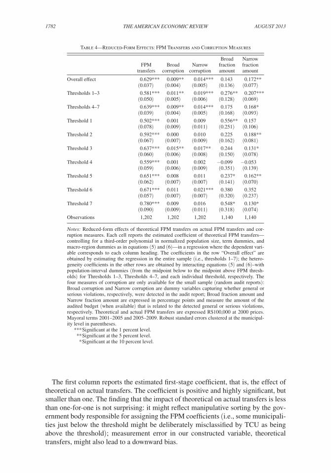
1782 THE AMERICAN ECONOMIC REVIEW AugusT 2013
The first column reports the estimated first-stage coefficient, that is, the effect of theoretical on actual transfers. The coefficient is positive and highly significant, but smaller than one. The finding that the impact of theoretical on actual transfers is less than one-for-one is not surprising: it might reflect manipulative sorting by the gov-ernment body responsible for assigning the FPM coefficients (i.e., some municipali-ties just below the threshold might be deliberately misclassified by TCU as being above the threshold); measurement error in our constructed variable, theoretical transfers, might also lead to a downward bias.
Table 4—Reduced-Form Effects: FPM Transfers and Corruption Measures
Broad NarrowFPM Broad Narrow fraction fraction
transfers corruption corruption amount amount
Overall effect 0.629*** 0.009** 0.014*** 0.143 0.172**(0.037) (0.004) (0.005) (0.136) (0.077)
Thresholds 1–3 0.581*** 0.011** 0.019*** 0.276** 0.207***(0.050) (0.005) (0.006) (0.128) (0.069)
Thresholds 4–7 0.639*** 0.009** 0.014*** 0.175 0.168*(0.039) (0.004) (0.005) (0.168) (0.093)
Threshold 1 0.502*** 0.001 0.009 0.556** 0.157(0.078) (0.009) (0.011) (0.251) (0.106)
Threshold 2 0.592*** 0.000 0.010 0.225 0.188**(0.067) (0.007) (0.009) (0.162) (0.081)
Threshold 3 0.637*** 0.015** 0.017** 0.244 0.131*(0.060) (0.006) (0.008) (0.150) (0.078)
Threshold 4 0.559*** 0.001 0.002 −0.099 −0.053(0.059) (0.006) (0.009) (0.351) (0.139)
Threshold 5 0.651*** 0.008 0.011 0.237* 0.162**(0.062) (0.007) (0.007) (0.141) (0.070)
Threshold 6 0.671*** 0.011 0.021*** 0.380 0.352(0.057) (0.007) (0.007) (0.320) (0.237)
Threshold 7 0.780*** 0.009 0.016 0.548* 0.130*(0.090) (0.009) (0.011) (0.318) (0.074)
Observations 1,202 1,202 1,202 1,140 1,140
Notes: Reduced-form effects of theoretical FPM transfers on actual FPM transfers and cor-ruption measures. Each cell reports the estimated coefficient of theoretical FPM transfers—controlling for a third-order polynomial in normalized population size, term dummies, and macro-region dummies as in equations (5) and (6)—in a regression where the dependent vari-able corresponds to each column heading. The coefficients in the row “Overall effect” are obtained by estimating the regression in the entire sample (i.e., thresholds 1–7); the hetero-geneity coefficients in the other rows are obtained by interacting equations (5) and (6)–with population-interval dummies (from the midpoint below to the midpoint above FPM thresh-olds) for Thresholds 1–3, Thresholds 4–7, and each individual threshold, respectively. The four measures of corruption are only available for the small sample (random audit reports): Broad corruption and Narrow corruption are dummy variables capturing whether general or serious violations, respectively, were detected in the audit report; Broad fraction amount and Narrow fraction amount are expressed in percentage points and measure the amount of the audited budget (when available) that is related to the detected general or serious violations, respectively. Theoretical and actual FPM transfers are expressed R$100,000 at 2000 prices. Mayoral terms 2001–2005 and 2005–2009. Robust standard errors clustered at the municipal-ity level in parentheses.
*** Significant at the 1 percent level. ** Significant at the 5 percent level. * Significant at the 10 percent level.
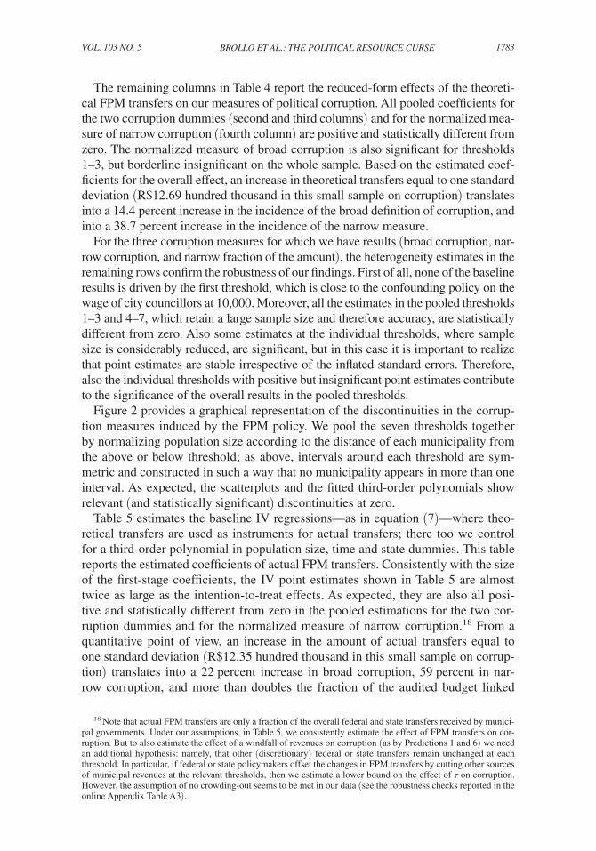
1783Brollo et al.: the Political resource curseVol. 103 No. 5
The remaining columns in Table 4 report the reduced-form effects of the theoreti-cal FPM transfers on our measures of political corruption. All pooled coefficients for the two corruption dummies (second and third columns) and for the normalized mea-sure of narrow corruption (fourth column) are positive and statistically different from zero. The normalized measure of broad corruption is also significant for thresholds 1–3, but borderline insignificant on the whole sample. Based on the estimated coef-ficients for the overall effect, an increase in theoretical transfers equal to one standard deviation (R$12.69 hundred thousand in this small sample on corruption) translates into a 14.4 percent increase in the incidence of the broad definition of corruption, and into a 38.7 percent increase in the incidence of the narrow measure.
For the three corruption measures for which we have results (broad corruption, nar-row corruption, and narrow fraction of the amount), the heterogeneity estimates in the remaining rows confirm the robustness of our findings. First of all, none of the baseline results is driven by the first threshold, which is close to the confounding policy on the wage of city councillors at 10,000. Moreover, all the estimates in the pooled thresholds 1–3 and 4–7, which retain a large sample size and therefore accuracy, are statistically different from zero. Also some estimates at the individual thresholds, where sample size is considerably reduced, are significant, but in this case it is important to realize that point estimates are stable irrespective of the inflated standard errors. Therefore, also the individual thresholds with positive but insignificant point estimates contribute to the significance of the overall results in the pooled thresholds.
Figure 2 provides a graphical representation of the discontinuities in the corrup-tion measures induced by the FPM policy. We pool the seven thresholds together by normalizing population size according to the distance of each municipality from the above or below threshold; as above, intervals around each threshold are sym-metric and constructed in such a way that no municipality appears in more than one interval. As expected, the scatterplots and the fitted third-order polynomials show relevant (and statistically significant) discontinuities at zero.
Table 5 estimates the baseline IV regressions—as in equation (7)—where theo-retical transfers are used as instruments for actual transfers; there too we control for a third-order polynomial in population size, time and state dummies. This table reports the estimated coefficients of actual FPM transfers. Consistently with the size of the first-stage coefficients, the IV point estimates shown in Table 5 are almost twice as large as the intention-to-treat effects. As expected, they are also all posi-tive and statistically different from zero in the pooled estimations for the two cor-ruption dummies and for the normalized measure of narrow corruption.18 From a quantitative point of view, an increase in the amount of actual transfers equal to one standard deviation (R$12.35 hundred thousand in this small sample on corrup-tion) translates into a 22 percent increase in broad corruption, 59 percent in nar-row corruption, and more than doubles the fraction of the audited budget linked
18 Note that actual FPM transfers are only a fraction of the overall federal and state transfers received by munici-pal governments. Under our assumptions, in Table 5, we consistently estimate the effect of FPM transfers on cor-ruption. But to also estimate the effect of a windfall of revenues on corruption (as by Predictions 1 and 6) we need an additional hypothesis: namely, that other (discretionary) federal or state transfers remain unchanged at each threshold. In particular, if federal or state policymakers offset the changes in FPM transfers by cutting other sources of municipal revenues at the relevant thresholds, then we estimate a lower bound on the effect of τ on corruption. However, the assumption of no crowding-out seems to be met in our data (see the robustness checks reported in the online Appendix Table A3).
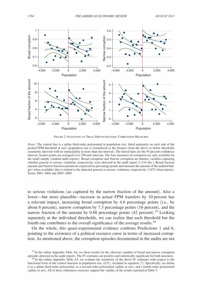
1784 THE AMERICAN ECONOMIC REVIEW AugusT 2013
to serious violations (as captured by the narrow fraction of the amount). Also a lower—but more plausible—increase in actual FPM transfers by 10 percent has a relevant impact, increasing broad corruption by 4.6 percentage points (i.e., by about 6 percent), narrow corruption by 7.3 percentage points (16 percent), and the narrow fraction of the amount by 0.88 percentage points (42 percent).19 Looking separately at the individual thresholds, we can realize that each threshold but the fourth one contributes to the overall significance of the average results.20
On the whole, this quasi-experimental evidence confirms Predictions 1 and 6, pointing to the existence of a political resource curse in terms of increased corrup-tion. As mentioned above, the corruption episodes documented in the audits are not
19 In the online Appendix Table A4, we show results for the (discrete) number of broad and narrow corruption episodes detected in the audit reports. The IV estimates are positive and statistically significant for both measures.
20 In the online Appendix Table A5, we evaluate the sensitivity of the above IV estimates with respect to the functional form of the control function in population size, G( P i ), included in equation (7). Specifically, we define it as a spline third-order polynomial, as a second-order polynomial (spline or not), and a fourth-order polynomial (spline or not). All of these robustness exercises support the validity of the results reported in Table 5.
0.6
0.7
0.8
0.9
1B
road
cor
rupt
ion
−4,000 −2,000 0 2,000 4,000
Population
0.2
0.3
0.4
0.5
0.6
Nar
row
cor
rupt
ion
−4,000 −2,000 0 2,000 4,000
Population
2
4
6
8
10
Bro
ad fr
actio
n of
the
amou
nt
−4,000 −2,000 0 2,000 4,000
Population
0
1
2
3
4
Nar
row
frac
tion
of th
e am
ount
−4,000 −2,000 0 2,000 4,000
Population
Figure 2. Intention-to-Treat Discontinuities: Corruption Measures
Notes: The central line is a spline third-order polynomial in population size, fitted separately on each side of the pooled FPM threshold at zero (population size is normalized as the distance from the above or below threshold; symmetric intervals with no municipality in more than one interval). The lateral lines are the 95 percent confidence interval. Scatter points are averaged over 250-unit intervals. The four measures of corruption are only available for the small sample (random audit reports): Broad corruption and Narrow corruption are dummy variables capturing whether general or serious violations, respectively, were detected in the audit report (1,134 obs.); Broad fraction amount and Narrow fraction amount are expressed in percentage points and measure the amount of the audited bud-get (when available) that is related to the detected general or serious violations, respectively (1,072 observations). Terms 2001–2005 and 2005–2009.
1785Brollo et al.: the Political resource curseVol. 103 No. 5
strictly related to the FPM transfers. Hence, the RD estimates document a general deterioration in the quality of the policy-making environment induced by the addi-tional revenues triggered by the FPM thresholds.21
B. Exploring the Mechanisms of the Effect of Transfers on Corruption
We are aware that the detected (reduced-form) effect of larger transfers on political corruption might arise from different mechanisms in our data. Our model
21 Note that the specifications in Tables 4 and 5 never include regressors referring to the quality of the oppo-nents. Hence, strictly speaking, these estimates correspond to a test of Prediction 6, what we called the “general equilibrium” effect of budget size on rents, namely the sum of the moral hazard effect (holding constant the quality of the opponents) and the interaction effect (when the quality of the opponents is endogenized). The estimates remain almost unchanged if we also control for the average education of the opponents, suggesting that the moral hazard effect is responsible for most if not all of the estimated effect of budget size on corruption. Nevertheless, this might reflect data limitations. When we use the small sample on corruption, the characteristics of opponents are balanced around the thresholds, suggesting that there might not be enough variation to disentangle the moral hazard from the interaction effect. These limitations notwithstanding, in the next section, we provide additional tests to shed more light on the mechanisms of the effect of larger transfers on corruption.
Table 5—IV Estimates: Corruption Measures
Broad NarrowBroad Narrow fraction fraction
corruption corruption amount amount
Overall effect 0.014** 0.022*** 0.220 0.265**(0.007) (0.008) (0.207) (0.118)
Thresholds 1–3 0.018** 0.031*** 0.447** 0.342***(0.008) (0.010) (0.211) (0.117)
Thresholds 4–7 0.014** 0.023*** 0.276 0.260*(0.007) (0.008) (0.245) (0.135)
Threshold 1 0.005 0.019 0.905** 0.294*(0.014) (0.018) (0.412) (0.177)
Threshold 2 0.003 0.017 0.397 0.309**(0.010) (0.013) (0.265) (0.133)
Threshold 3 0.022** 0.026** 0.380* 0.208*(0.009) (0.011) (0.221) (0.114)
Threshold 4 0.004 0.007 −0.066 −0.030(0.010) (0.015) (0.504) (0.202)
Threshold 5 0.012 0.018* 0.362* 0.242**(0.010) (0.010) (0.210) (0.105)
Threshold 6 0.016 0.030*** 0.540 0.489(0.010) (0.011) (0.433) (0.317)
Threshold 7 0.012 0.020 0.666* 0.174*(0.011) (0.014) (0.361) (0.090)
Observations 1,202 1,202 1,140 1,140
Notes: Effects of FPM transfers on corruption measures. Each cell reports the estimated coef-ficient of actual FPM transfers (instrumented with theoretical FPM transfers)—controlling for a third-order polynomial in normalized population size, term dummies, and macro-region dummies as in equation (7)—in a regression where the dependent variable corresponds to each column heading. Robust standard errors clustered at the municipality level are in parentheses. See notes to Table 4 for a description of the variables.
*** Significant at the 1 percent level. ** Significant at the 5 percent level. * Significant at the 10 percent level.
1786 THE AMERICAN ECONOMIC REVIEW AugusT 2013
of political agency, however, has two more specific predictions, which can help discriminate between our explanation and others. First, the central mechanism driv-ing the theoretical results bears the following implication (highlighted in the first part of Prediction 1): an incumbent who receives a larger budget faces a weaker electoral punishment for corruption. Second, as highlighted by Prediction 3, higher transfers increase corruption by more if the opponents are less educated. In this sec-tion, we test these additional implications of the theory.
To test the first part of Prediction 1, as discussed in Section IIIC, we combine our fuzzy RD design with the identification strategy used by Ferraz and Finan (2008), and estimate equation (8) in order to compare the electoral punishment of disclosed corruption just above and below the FPM thresholds. Table 6 reports the results for two different electoral outcomes: a dummy equal to one if the incumbent decides to run for reelection (panel A) and a dummy equal to one if the incumbent is reelected, conditional on running for reelection (panel B) and unconditionally for the whole sample (panel C). To make the interpretation of the results starker, we follow Ferraz and Finan (2008) and restrict the sample to incumbents who are eligible for reelec-tion (that is, those who do not face a binding term limit). To save on space, we do not report all regressors included in equation (8). Indeed, the coefficients of interest are two. First, the interaction between before (which indicates if the audit report has been released before the next election) and one of our corruption measures (specified in each column heading) captures the impact of disclosing corruption on the probability of rerunning or being reelected (that is, the punishment of corruption). Second, the (triple) interaction between these two variables and our theoretical FPM transfers captures whether the punishment of corruption is differentially lower just above the FPM thresholds, as we also control for a third-order polynomial in population size and its multiple interactions with corruption and the timing of the audit release.
The main effect of interest is the “net” effect on whether the (eligible) incum-bent is reelected or not (panel C). The other panels, however, provide evidence on the mechanical interpretation of whether this net reelection effect arises from the decision by the incumbent (or the party leadership) not to rerun (panel A), or from the lower electoral chances of the incumbent who decides to rerun anyway (panel B).
Panel C of Table 6 shows that, as expected, incumbent mayors whose corrup-tion has been disclosed before the next election have a lower probability of being reelected according to all our measures of corruption (as shown by the interaction coefficients between the “before” dummy and each corruption measure). At the same time, this effect of disclosed corruption is lower (that is, the probability of being reelected is higher) if FPM transfers are larger, as shown by the triple interaction coefficients in the first row of panel C. Interestingly, this last effect is statistically significant only for the two measures capturing more severe episodes of corrup-tion: that is, the narrow corruption dummy and the narrow fraction of the amount. According to the estimates in the fourth column of panel C of Table 6, an increase in the amount of the audited budget linked to narrow corruption episodes equal to one standard deviation (1.84 percentage points) reduces the probability of being reelected by 17.5 percentage points (that is, by about 43 percent with respect to the average of 40.7 percentage points for eligible incumbents). This punishment of disclosed corruption is dampened when transfers are larger, because an increase in theoretical FPM transfers equal to one standard deviation (R$1.317 million) reduces
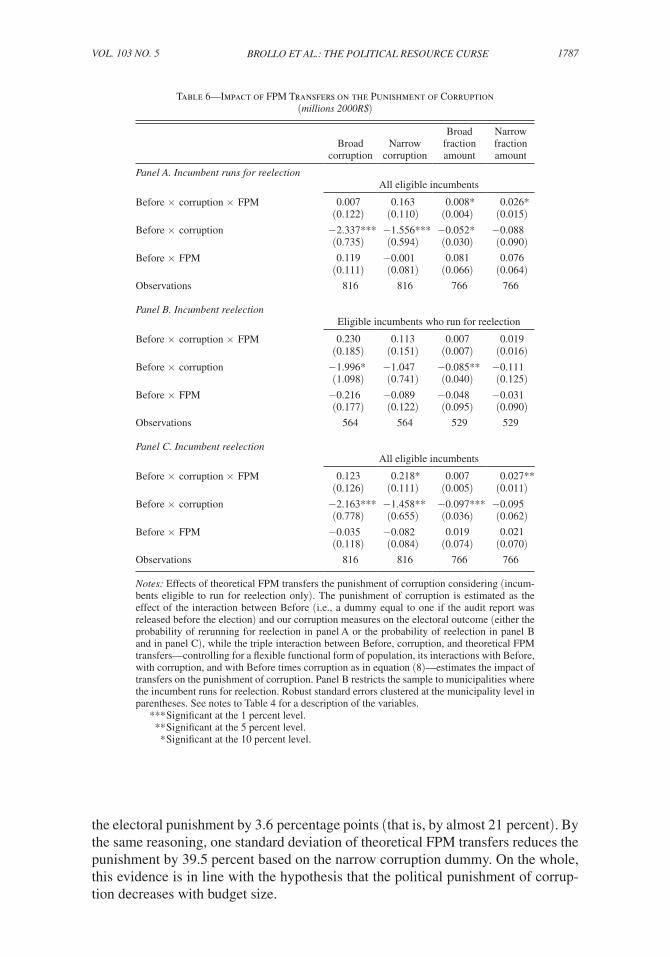
1787Brollo et al.: the Political resource curseVol. 103 No. 5
the electoral punishment by 3.6 percentage points (that is, by almost 21 percent). By the same reasoning, one standard deviation of theoretical FPM transfers reduces the punishment by 39.5 percent based on the narrow corruption dummy. On the whole, this evidence is in line with the hypothesis that the political punishment of corrup-tion decreases with budget size.
Table 6—Impact of FPM Transfers on the Punishment of Corruption (millions 2000R$)
Broad NarrowBroad Narrow fraction fraction
corruption corruption amount amount
Panel A. Incumbent runs for reelectionAll eligible incumbents
Before × corruption × FPM 0.007 0.163 0.008* 0.026*(0.122) (0.110) (0.004) (0.015)
Before × corruption −2.337*** −1.556*** −0.052* −0.088(0.735) (0.594) (0.030) (0.090)
Before × FPM 0.119 −0.001 0.081 0.076(0.111) (0.081) (0.066) (0.064)
Observations 816 816 766 766
Panel B. Incumbent reelectionEligible incumbents who run for reelection
Before × corruption × FPM 0.230 0.113 0.007 0.019(0.185) (0.151) (0.007) (0.016)
Before × corruption −1.996* −1.047 −0.085** −0.111(1.098) (0.741) (0.040) (0.125)
Before × FPM −0.216 −0.089 −0.048 −0.031(0.177) (0.122) (0.095) (0.090)
Observations 564 564 529 529
Panel C. Incumbent reelectionAll eligible incumbents
Before × corruption × FPM 0.123 0.218* 0.007 0.027**(0.126) (0.111) (0.005) (0.011)
Before × corruption −2.163*** −1.458** −0.097*** −0.095(0.778) (0.655) (0.036) (0.062)
Before × FPM −0.035 −0.082 0.019 0.021(0.118) (0.084) (0.074) (0.070)
Observations 816 816 766 766
Notes: Effects of theoretical FPM transfers the punishment of corruption considering (incum-bents eligible to run for reelection only). The punishment of corruption is estimated as the effect of the interaction between Before (i.e., a dummy equal to one if the audit report was released before the election) and our corruption measures on the electoral outcome (either the probability of rerunning for reelection in panel A or the probability of reelection in panel B and in panel C), while the triple interaction between Before, corruption, and theoretical FPM transfers—controlling for a flexible functional form of population, its interactions with Before, with corruption, and with Before times corruption as in equation (8)—estimates the impact of transfers on the punishment of corruption. Panel B restricts the sample to municipalities where the incumbent runs for reelection. Robust standard errors clustered at the municipality level in parentheses. See notes to Table 4 for a description of the variables.
*** Significant at the 1 percent level. ** Significant at the 5 percent level. * Significant at the 10 percent level.
1788 THE AMERICAN ECONOMIC REVIEW AugusT 2013
The other evidence reported in Table 6 aims at disentangling whether the above reelection punishment is driven by the (endogenous) choice to rerun, or by the lower reelection chances of those incumbents who decide to rerun. Based on the statistical significance of the results, one may conclude that the main driver of the reelection effect is the decision by the incumbent whether to rerun or not: only in panel A the triple interaction turns out to be statistically significant. It seems that mayors who are under fire because of alleged irregularities decide to retire, or are forced to do so by their political party. It is natural to interpret this withdrawal as occurring in anticipation of punishment by the voters if they stood for reelection. In other words, mayors (or their political parties) seem to anticipate the electoral punishment once corruption is disclosed before the next election.22 Panel B, how-ever, also reports triple interaction coefficients consistently positive and with siz-able magnitude, although they are borderline insignificant. This means that they also contribute to the (increased) significance of the net reelection effect discussed above. At the end of the day, although this evidence is less accurately estimated, also for incumbents who decide to rerun, the electoral punishment is attenuated by larger transfers.
Furthermore, to test Prediction 3, namely that the effect of transfers on cor-ruption is enhanced if the opponent is of low quality, in Table 7 we interact the baseline IV specification in equation (7) with the fraction of opponents with col-lege degree and their average years of schooling. To control for other city-specific characteristics potentially correlated with the education of politicians, we also control for some covariates and their interaction with FPM transfers. In particular, we include as covariates the average income, the literacy rate, and the urbanization rate at the municipality level. To save on space, we only report the coefficients of actual FPM transfers and their interaction with the politicians’ education mea-sures, and omit the threshold-by-threshold estimates. The results reported in this table confirm our prediction: the effect of larger FPM transfers on corruption is consistently attenuated by the presence of high quality opponents. For instance, an increase in the opponents’ years of schooling equal to one standard deviation (2.622) reduces the impact of FPM transfers on the incidence of both broad and narrow corruption by about 7 percent, and on the narrow fraction of the amount by about 8 percent.
Finally, our model bears an additional implication (Prediction 2): high quality mayors extract less rents, because by assumption they face a higher cost if caught, compared to low quality mayors. This prediction cannot be directly tested with a robust identification strategy, because the observed education of the mayor is not random. Nevertheless, sample correlations are strongly consistent with this implica-tion. The incidence of narrow corruption is 0.49 among mayors without a college degree versus 0.41 among mayors with a college degree (difference significant at a 5 percent level), and the average fraction of the audited budget linked to narrow corruption violations is 2.3 percentage points for mayors without a college degree
22 This anticipated punishment is consistent with anecdotal evidence on Brazilian politics. In recent years, the Brazilian press has repeatedly reported cases of potential candidates who have been ousted by their party because of alleged corruption charges, or even of mayors impeached by city councils because of the same reason. The major political parties have also approved internal rules denying the right to be a candidate in similar cases.
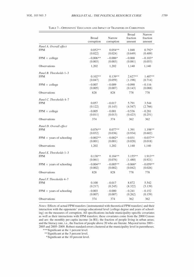
1789Brollo et al.: the Political resource curseVol. 103 No. 5
Table 7—Opponents’ Education and Impact of Transfers on Corruption
Broad NarrowBroad Narrow fraction fraction
corruption corruption amount amount
Panel A. Overall effectFPM 0.052** 0.054** 1.048 0.792*
(0.022) (0.024) (0.649) (0.409)FPM × college −0.006** −0.006* −0.068 −0.103*
(0.003) (0.003) (0.081) (0.053)Observations 1,202 1,202 1,140 1,140
Panel B. Thresholds 1–3FPM 0.102** 0.139** 2.627** 1.407**
(0.047) (0.059) (1.198) (0.714)FPM × college −0.007 −0.009 −0.090 −0.116
(0.005) (0.007) (0.143) (0.088)Observations 828 828 778 778
Panel C. Thresholds 4–7FPM 0.057 −0.017 5.791 3.544
(0.122) (0.143) (4.547) (2.766)FPM × college −0.005 −0.001 −0.536 −0.281
(0.011) (0.013) (0.423) (0.251)Observations 374 374 362 362
Panel D. Overall effectFPM 0.076** 0.077** 1.391 1.198**
(0.032) (0.036) (0.934) (0.602)FPM × years of schooling −0.002** −0.002* −0.031 −0.037**
(0.001) (0.001) (0.028) (0.018)Observations 1,202 1,202 1,140 1,140
Panel E. Thresholds 1–3FPM 0.138** 0.184** 3.155** 1.913**
(0.061) (0.076) (1.480) (0.921)FPM × years of schooling −0.004** −0.005** −0.068* −0.059**
(0.002) (0.002) (0.042) (0.026)Observations 828 828 778 778
Panel F. Thresholds 4–7FPM 0.100 −0.017 8.872 5.542
(0.217) (0.245) (8.322) (5.139)FPM × years of schooling −0.003 −0.000 −0.241 −0.152
(0.007) (0.007) (0.262) (0.159)Observations 374 374 362 362
Notes: Effects of actual FPM transfers (instrumented with theoretical FPM transfers) and their interaction with the opponents’ average educational level (college degree and years of school-ing) on the measures of corruption. All specifications include municipality-specific covariates as well as their interactions with FPM transfers; these covariates come from the 2000 Census and are: the monthly per capita income (in R$); the fraction of people living in urban areas; and the literacy rate, i.e., the fraction of people above 20 who are literate. Mayoral terms 2001–2005 and 2005–2009. Robust standard errors clustered at the municipality level in parentheses.
*** Significant at the 1 percent level. ** Significant at the 5 percent level. * Significant at the 10 percent level.
1790 THE AMERICAN ECONOMIC REVIEW AugusT 2013
versus 1.6 for mayors with a college degree (difference significant at a 10 percent level). These differences are even larger and more statistically significant away from the population thresholds (where the mayor’s type is less likely to be endogenous with respect to the amount of FPM transfers).23
C. The Effect of Federal Transfers on Political Selection
Next, we study the effect of transfers on the quality of political opponents (Prediction 4) and on the incumbent’s reelection (Prediction 5). As explained in Section IIC, to stay close to our model, we restrict the sample to municipalities where the mayor decides to run for reelection, because only there we have a clear measure of the opponents’ quality. This sample is larger than that on corruption, because it also includes municipalities that were not audited.24
Table 8 reports the first-stage and reduced-form regressions, and the estimated coefficients refer to theoretical FPM transfers; Table 9 reports the IV estimates, where the coefficients refer to actual FPM transfers. In all of these tables, larger (theoretical or actual) transfers lead to a deterioration in the average quality of the opponents—as measured by their education—and to an increase in the probabil-ity that the incumbent is reelected. In particular, according to the IV estimates in Table 9 for the entire sample (thresholds 1–7), an increase in actual FPM transfers equal to one standard deviation (R$12.64 hundred thousand in this large sam-ple on political selection) translates into a 23 percent reduction in the fraction of opponents with a college degree, an 8 percent reduction in their average years of schooling, and a 26 percent increase in the incumbent’s probability of reelec-tion. Analogously, a 10 percent increase in actual transfers induces a 6 percent drop in college, 2 percent in years of schooling, and 7 percent increase in the reelection probability.25
The threshold-by-threshold heterogeneity estimates in the remaining columns of Table 9 show that all thresholds contribute to the significance of the overall results. However, the point estimates are larger for lower thresholds; indeed, the negative impact of federal transfers on opponents’ education is three times as large in thresholds 1–3 than in thresholds 4–7. Although this could simply be due to sample noise, it is tempting to speculate that the political arena changes along with local characteristics. In small municipalities, for instance, the positive impact of money on the incumbent’s reelection might be larger because in big towns the
23 For instance, by dropping municipalities in a neighborhood from −500 to +500 inhabitants around each threshold, the incidence of narrow corruption is 0.49 among mayors without a college degree versus 0.40 among mayors with a college degree (difference significant at a 1 percent level), and the average fraction of the audited budget linked to narrow corruption violations is 2.4 percentage points for mayors without a college degree versus 1.5 for mayors with a college degree (difference significant at a 5 percent level). Similar results apply by dropping different population intervals around the population thresholds (available upon request).
24 The online Appendix Table A7 does not restrict the sample to municipalities where the incumbent runs for reelection, and shows that the negative effect of transfers on politicians’ education also holds in the larger sample of all candidates (including elected mayors) in all municipalities, as well as with alternative definitions of who is the opponent (e.g., only the most popular opponents, or all the opponents of the political party of the incumbent).
25 As the current FPM revenue-sharing mechanism has been in place since 1981, one could be afraid of a general-equilibrium effect of transfers on politicians’ education through the channel of citizens’ education. Note that, the effect of transfers on schooling levels being positive (see Litschig 2008a), this would result in our estimates to be a lower bound of the direct effect of transfers on politicians’ education. Furthermore, our estimates are not sensitive to the inclusion of the municipal literacy rate as an additional control (results available upon request).
1791Brollo et al.: the Political resource curseVol. 103 No. 5
incumbency advantage tends to be higher per se, due to higher barriers to entry for challengers.26
Figure 3 provides a graphical representation of the discontinuities in the political variables induced by the FPM policy (the intention-to-treat effects). As we have done in Figure 2 for the corruption measures, we pool the seven thresholds together to gain sample size. The two education variables show a clear tendency to grow both before and after the normalized threshold, but the discontinuity at zero is both clearly visible in the scatterplots and statistically significant, like the jump in the
26 Table A6 in the online Appendix shows that the baseline IV results are robust to different functional form assumptions on the control function G( P i ) in equation (7).
Table 8—Reduced-Form Effects: FPM Transfers, Opponents’ Education, and Election Outcome
FPM Years of Incumbenttransfers College schooling reelection
Overall effect 0.732*** −0.006** −0.056*** 0.009***(0.024) (0.003) (0.019) (0.003)
Thresholds 1–3 0.638*** −0.011*** −0.099*** 0.008*(0.028) (0.004) (0.027) (0.005)
Thresholds 4–7 0.753*** −0.005* −0.041** 0.006*(0.029) (0.003) (0.020) (0.004)
Threshold 1 0.540*** −0.005 −0.063 0.018**(0.044) (0.006) (0.048) (0.007)
Threshold 2 0.552*** −0.016*** −0.141*** 0.010(0.039) (0.006) (0.038) (0.006)
Threshold 3 0.657*** −0.011** −0.091*** 0.006(0.031) (0.005) (0.032) (0.006)
Threshold 4 0.681*** −0.006 −0.032 0.009(0.038) (0.005) (0.031) (0.006)
Threshold 5 0.693*** −0.005 −0.050* 0.009(0.040) (0.004) (0.028) (0.006)
Threshold 6 0.834*** −0.005 −0.050* 0.009(0.058) (0.005) (0.028) (0.006)
Threshold 7 0.778*** 0.001 −0.010 0.000(0.053) (0.005) (0.034) (0.007)
Observations 2,877 2,877 2,877 2,877
Notes: Reduced-form effects of theoretical FPM transfers on actual FPM transfers, character-istics of the pool of opponents, and the election outcome. Each cell reports the estimated coef-ficient of theoretical FPM transfers—controlling for a third-order polynomial in normalized population size, term dummies, and macro-region dummies as in equations (5) and (6)—in a regression where the dependent variable corresponds to each column heading. The coeffi-cients in the row “Overall effect” are obtained by estimating the regression in the entire sample (i.e., thresholds 1–7); the heterogeneity coefficients in the other rows are obtained by inter-acting equations (5) and (6) with population-interval dummies (from the midpoint below to the midpoint above FPM thresholds) for Thresholds 1–3, Thresholds 4–7, and each individual threshold, respectively. The political variables are available for the large sample (where the incumbent runs for reelection): College is the fraction of opponents holding a college degree; Years of schooling measures the opponent’s average years of schooling; Incumbent reelection is the probability of the incumbent being reappointed. Theoretical and actual FPM transfers are expressed in R$100,000 at 2000 prices. Mayoral terms 2001–2005 and 2005–2009. Robust standard errors clustered at the municipality level in parentheses.
*** Significant at the 1 percent level. ** Significant at the 5 percent level. * Significant at the 10 percent level.
1792 THE AMERICAN ECONOMIC REVIEW AugusT 2013
(spline) third-order polynomials. The same holds for the jump in the incumbent’s reelection probability.
On the whole, this quasi-experimental evidence strongly confirms Predictions 4 and 5, pointing to an additional detrimental effect of windfall resources on the qual-ity of politicians and the degree of political competition.27
D. Discussion
In principle, there are other mechanisms that might interact with our results and contribute to explain the impact of larger transfers on both corruption and political selection. These alternative channels, however, are rejected by both the institutional
27 The theory predicts that, in the long run, the equilibrium quality of elected mayors also deteriorates with larger transfers, both because they are selected from a worse pool of candidates, and because voters have a lower quality threshold for replacing the incumbent. The evidence is not conclusive, however: when estimating the same baseline specifications on the education of elected mayors, FPM transfers have the expected negative signs but are not statisti-cally significant. This may reflect the short time span since the introduction of the audits, which started in 2003. Before the audits were in place, voters had less accurate information and they may have been less focused on corruption.
Table 9—IV Estimates: Opponents’ Education and Election Outcome
Years of IncumbentCollege schooling reelection
Overall effect −0.008** −0.077*** 0.012***(0.004) (0.026) (0.005)
Thresholds 1–3 −0.017*** −0.150*** 0.013*(0.006) (0.041) (0.007)
Thresholds 4–7 −0.007* −0.055** 0.008*(0.004) (0.026) (0.005)
Threshold 1 −0.009 −0.111 0.029**(0.010) (0.079) (0.012)
Threshold 2 −0.026*** −0.231*** 0.018*(0.009) (0.064) (0.011)
Threshold 3 −0.016** −0.132*** 0.010(0.007) (0.048) (0.008)
Threshold 4 −0.009 −0.051 0.013(0.006) (0.045) (0.008)
Threshold 5 −0.007 −0.073* 0.013(0.006) (0.040) (0.008)
Threshold 6 −0.006 −0.061* 0.011(0.006) (0.032) (0.007)
Threshold 7 0.000 −0.018 0.001(0.006) (0.042) (0.009)
Observations 2,877 2,877 2,877
Notes: Effects of FPM transfers on the characteristics of the pool of opponents and the election outcome. Each cell reports the estimated coefficient of actual FPM transfers (instrumented with theoretical FPM transfers)—controlling for a third-order polynomial in normalized population size, term dummies, and macro-region dummies as in equation (7)—in a regression where the dependent variable corresponds to each column heading. See notes to Table 8 for a description of the variables.
*** Significant at the 1 percent level. ** Significant at the 5 percent level. * Significant at the 10 percent level.
1793Brollo et al.: the Political resource curseVol. 103 No. 5
analysis of the Brazilian context and by additional tests performed on our data. There are two types of channels that we need to reject: “mechanical” channels based on the audit technology and “political” channels different from those identified in a political agency framework.
First, it might be the case that the audits on which our measures of corruption are based might be more carefully done in municipalities with a larger budget. Alternatively, a larger budget might require more employees and each of them might have an opportunity to grab rents. These and other “mechanical”explanations of the FPM effect are at odds with the audit technology discussed in Section IIB, however. The quality of the audit report is not linked to the size of the budget (as more time or auditors are devoted to municipalities with larger budgets). Our results are also based on normalized measures of the incidence of detected corruption, which can accommodate for this concern. Furthermore, the corruption episodes are linked to the actions of elected officials (see the online Appendix for more details), and they are not related to the number of employees in the municipal government.
Second, it might be the case that a larger budget favors parties with a specific ideological orientation, and these parties might be associated with differential levels of corruption or patterns of political selection. Alternatively, mayors with a larger
0.35
0.4
0.45
0.5
0.55
0.6C
olle
ge
−4,000 −2,000 0 2,000 4,000
Population
11
11.5
12
12.5
13
Yea
rs o
f sch
oolin
g
−4,000 −2,000 0 2,000 4,000
Population
0.5
0.55
0.6
0.65
0.7
Incu
mbe
nt r
eele
ctio
n
−4,000 −2,000 0 2,000 4,000
Population
Figure 3. Intention-to-Treat Discontinuities: Opponents’ Education and Election Outcome
Notes: See notes to Figure 2. The political variables are available for the large sample (where the incumbent runs for reelection): College is the fraction of opponents holding a college degree; Years of schooling measures the opponent’s average years of schooling; Incumbent reelection is the probability of the incumbent being reappointed (2,877 obs.). Terms 2001–2005 and 2005–2009.
1794 THE AMERICAN ECONOMIC REVIEW AugusT 2013
budget might be able to mobilize more resources in their reelection campaign. These alternative “political” channels of the FPM effect are rejected by our data. In the online Appendix Table A2, we test for the continuity of potentially endogenous variables around the FPM cutoffs. In particular, we look at the political orienta-tion of the mayor (captured by the party he belongs to) and the campaign funds he used (in addition to the total campaign funds, we also have detailed information on firms’ donations, candidate’s own funds, and other types of donations). All of these potentially endogenous variables are balanced around the FPM cutoffs, ruling out the existence of these alternative political channels.
V. Conclusion
Could a windfall of resources deteriorate the quality of the political process? And if so, how does this happen? These are important questions, because lagging regions or countries often receive additional funds from higher levels of government or from international organizations, to make up for their underdevelopment. Since, accord-ing to a large literature, a common cause of economic backwardness is precisely the poor functioning of government institutions, the risk that these additional resources could be counterproductive cannot be neglected.
Here, we have focused on two mechanisms that are of fundamental importance in a variety of situations: the effects of additional resources on political corruption and on the incentives to participate in politics. At the margin, higher exogenous revenues induce more corruption, because incumbents have more rooms to grab rents without disappointing voters. Moreover, if the benefit of corruption is more valuable to those with worse outside options, individuals of lower quality are attracted into politics. The interaction between these two effects gives rise to a complementarity: precisely because his opponents are now of lower quality, an incumbent can afford to grab more rents while at the same time increasing his reelection chances.
In light of these (theoretical) results, we have investigated a specific Brazilian institution that provides an ideal quasi-experimental setting. We found considerable support for the implications of the theory. In particular, a 10 percent increase in the federal transfers to municipal governments raises local corruption by 6 percent (broad definition, possibly including bad administration) or by 16 percent (nar-row definition, with only severe violation episodes). Moreover, this fiscal windfall increases the incumbent mayor’s probability of reelection by 7 percent, and shrinks the fraction of his opponents with a college degree by 6 percent. Also in accordance with the theoretical predictions, the electoral punishment of disclosed corruption is found to be lower when federal transfers are larger.
On the whole, our empirical findings point to the existence of what we call a “political resource curse,” that is, a negative impact of windfall resources on political corruption and political selection. The term “curse” only refers to the detrimental channel that we identify in this paper. Our results are not inconsistent with higher transfers to municipalities increasing the quantity and quality of pub-lic services provided to the local population. For instance, Litschig (2008a), in the same quasi-experimental setting we use, finds that an exogenous increase in funds to Brazilian local governments raises spending on public education and improves literacy rates. Nevertheless, our evidence suggests that these specific benefits are
1795Brollo et al.: the Political resource curseVol. 103 No. 5
accompanied by a general deterioration in the functioning of the political process at the municipal level.
How general are these results, and in particular could they extend to other coun-tries and situations? Only additional research can answer this question. The causal effect identified by our strategy is estimated in a very specific setting: Brazilian municipalities that are similar in size and other characteristics. The high frequency of abuses detected by the audits suggests that Brazilian municipalities are a frag-ile institutional environment, where political agency problems are widespread. It could be that a windfall of resources would not have the same deleterious effects in other contexts, such as societies with a long tradition of good government and with abundant social capital. Nevertheless, additional resources are often given pre-cisely to regions or countries with weak institutions, like in the case of Structural Funds to lagging regions in the European Union, or of foreign aid to developing countries. As a result of these policies, and if our estimates have external validity, these already weak institutions might become even weaker.
REFERENCES
Angrist, Joshua D., Guido W. Imbens, and Donald B. Rubin. 1996. “Identification of Causal Effects Using Instrumental Variables.” Journal of the American Statistical Association 91 (434): 444–55.
Barro, Robert. 1973. “ The Control of Politicians: An Economic Model.” Public Choice 14: 19–42.Baumol, William J. 1990. “Entrepreneurship: Productive, Unproductive, and Destructive.” Journal of
Political Economy 98 (5): 893–921.Besley, Timothy. 2004. “Paying Politicians: Theory and Evidence.” Journal of the European Economic
Association 2 (2–3): 193–215.Besley, Timothy J., and Torsten Persson. 2008. “The Incidence of Civil War: Theory and Evidence.”
National Bureau of Economic Research Working Paper 14585.Besley, Timothy, and Michael Smart. 2007. “Fiscal Restraints and Voter Welfare.” Journal of Public
Economics 91 (3–4): 755–73.Brollo, Fernanda. 2011. “Why Do Voters Punish Corrupt Politicians? Evidence from the Brazilian
Anti-corruption Program.” Unpublished.Brollo, Fernanda, Tommaso Nannicini, Roberto Perotti, and Guido Tabellini. 2013. “The Political
Resource Curse: Dataset.” American Economic Review. http://dx.doi.org/10.1257/aer.103.5.1759.Brollo, Fernanda, and Ugo Troiano. 2012. “What Happens When a Woman Wins an Election? Evi-
dence from Close Races in Brazil.” Unpublished.Caselli, Francesco, and Wilbur John Coleman, II. 2011. “On the Theory of Ethnic Conflict.” Unpub-
lished.Caselli, Francesco, and Guy Michaels. 2011. “Do Oil Windfalls Improve Living Standards? Evidence
from Brazil.” Unpublished.Caselli, Francesco, and Massimo Morelli. 2004. “Bad Politicians.” Journal of Public Economics
88 (3–4): 759–82.Diermeier, Daniel, Michael Keane, and Antonio Merlo. 2005. “A Political Economy Model of Con-
gressional Careers.” American Economic Review 95 (1): 347–73.Ferejohn, John A. 1986. “Incumbent Performance and Electoral Control.” Public Choice 50 (1-3):
5–25.Ferraz, Claudio, and Frederico Finan. 2008. “Exposing Corrupt Politicians: The Effects of Bra-
zil’s Publicly Released Audits on Electoral Outcomes.” Quarterly Journal of Economics 123 (2): 703–45.
Ferraz, Claudio, and Frederico Finan. 2009. “Motivating Politicians: The Impacts of Monetary Incen-tives on Quality and Performance.” National Bureau of Economic Research Working Paper 14906.
Ferraz, Claudio, and Frederico Finan. 2011. “Electoral Accountability and Corruption: Evidence from the Audits of Local Governments.” American Economic Review 101 (4): 1274–311.
Gagliarducci, Stefano, and Tommaso Nannicini. 2013. “Do Better Paid Politicians Perform Better? Disentangling Incentives from Selection.” Journal of the European Economic Association 11 (2): 369–98.
1796 THE AMERICAN ECONOMIC REVIEW AugusT 2013
Gagliarducci, Stefano, Tommaso Nannicini, and Paolo Naticchioni. 2010. “Moonlighting Politicians.” Journal of Public Economics 94 (9–10): 688–99.
Galasso, Vincenzo, and Tommaso Nannicini. 2011. “Competing on Good Politicians.” American Politi-cal Science Review 105 (1): 79–99.
Hahn, Jinyong, Petra Todd, and Wilbert Van der Klaauw. 2001. “Identification and Estimation of Treatment Effects with a Regression-Discontinuity Design.” Econometrica 69 (1): 201–09.
Instituto Brasileiro de Geografia e Estatística. 2000–2007. “Estimativas da População.” http://ibge.gov.br/home/default.php (accessed February 12, 2009).
La Ferrara, Eliana, Alberto Chong, and Suzanne Duryea. 2008. “Soap Operas and Fertility: Evidence from Brazil.” Unpublished.
Litschig, Stephan. 2008a. “Intergovernmental Transfers and Elementary Education: Quasi-Experimen-tal Evidence from Brazil.” Unpublished.
Litschig, Stephan. 2008b. “Rules versus Political Discretion: Evidence from Constitutionally Guaran-teed Transfers to Local Governments in Brazil.” Department of Economics and Business, Universi-tat Pompeu Fabra, Economics Working Paper 1143.
Litschig, Stephan, and Kevin Morrison. 2009. “Electoral Effects of Fiscal Transfers: Quasi-Experi-mental Evidence from Local Executive Elections in Brazil, 1982–1988.” Unpublished.
Litschig, Stephan, and Yves Zamboni. 2012. “Judicial Presence and Rent Extraction.” Unpublished.Mattozzi, Andrea, and Antonio Merlo. 2008. “Political Careers or Career Politicians?” Journal of Pub-
lic Economics 92 (3–4): 597–608.McCrary, Justin. 2008. “Manipulation of the Running Variable in the Regression Discontinuity
Design: A Density Test.” Journal of Econometrics 142 (2): 698–714.Messner, Matthias, and Mattias K. Polborn. 2004. “Paying Politicians.” Journal of Public Economics
88 (12): 2423–45.Murphy, Kevin M., Andrei Shleifer, and Robert W. Vishny. 1991. “The Allocation of Talent: Implica-
tions for Growth.” Quarterly Journal of Economics 106 (2): 503–30.Persson, Torsten, and Guido Tabellini. 2000. Political Economics: Explaining Economic Policy. Cam-
bridge, MA: MIT Press.Robinson, James A., Ragnar Torvik, and Thierry Verdier. 2006. “Political Foundations of the Resource
Curse.” Journal of Development Economics 79 (2): 447–68.Ross, Michael. 2006. “A Closer Look at Oil, Diamonds, and Civil War.” Annual Review of Political
Science 9: 265–300.Rossi, Nicola. 2006. Mediterraneo del Nord: Un’altra idea del Mezzogiorno. Rome: Laterza.Tesouro Nacional. 2001–2003 and 2005–2007. “Fundo de Participação dos Municípios.”http://www.
tesouro.fazenda.gov.br/estados_municipios/index.asp (accessed February 12, 2009).Tornell, Aaron, and Philip R. Lane. 1999. “The Voracity Effect.” American Economic Review 89 (1):
22–46.Tribunal Superior Eleitoral. 2000–2008. “Repositorio de Dados: Candidatos.” http://www.tse.gov.br/
internet/index.html (accessed February 12, 2009).Tribunal Superior Eleitoral. 2000–2008. “Resultados Eleitorais.” http://www.tse.gov.br/internet/
index.html (accessed February 12, 2009).Velasco, Andres. 1999. “A Model of Endogenous Fiscal Deficits and Delayed Fiscal Reforms.” In Fis-
cal Institutions and Fiscal Performance, edited by James M. Poterba and Jürgen von Hagen, 37–58. Chicago: University of Chicago Press.
Vicente, Pedro C. 2010. “Does Oil Corrupt? Evidence from a Natural Experiment in West Africa.” Journal of Development Economics 92 (1): 28–38.
This article has been cited by:
1. Stephan Litschig,, Kevin M. Morrison. 2013. The Impact of Intergovernmental Transfers onEducation Outcomes and Poverty Reduction. American Economic Journal: Applied Economics 5:4,206-240. [Abstract] [View PDF article] [PDF with links]


![Nature’s blessing or nature’s curse [EBRD - Working papers]€¦ · Nature’s blessing or nature’s curse: the political economy of transition in resource-based economies Akram](https://img.pdfslide.net/doc/110x75/5b14edd87f8b9a467c8ccd5d/natures-blessing-or-natures-curse-ebrd-working-papers-natures-blessing.jpg)